Analysis of the form factors of B_c → D^(*), D_s^(*) and relevant nonleptonic decays

The pseudoscalar meson $ B_c $, which is composed of two heavy quarks with different flavours, is an excellent laboratory to study B physics. Because each heavy quark in the $ B_c $ meson can decay individually with the other acting as a spectator, $ B_c $is expected to have more rich decay channels than other B mesons. Moreover, it was estimated that the inclusive production cross section of the$ B_c $ meson including its excited states at the LHC is at a level of $ 1~\mu\rm b $ for $ \sqrt{14} $ TeV. This means that $ O(10^9) $ $ B_c $ mesons can be anticipated with 1 fb$ ^{-1} $ [1]. A similar viewpoint was also presented in Ref. [2]. Thus, the abundant events in experiments have encouraged physicists to pay more attention to them.

$ B_c $ is the lowest bound state consisting of b and c quarks and lies below the threshold of decaying into the pair of B and D mesons. Thus, pure electromagentic and strong decaying processes with flavor conservation are forbidden. $ B_c $ can only decay according to weak interaction and is comparatively long-lived. The $ B_c $ meson exhibits three distinct decay channels: (i) decay of the b-quark with the c-quark acting as a spectator, (ii) decay of the c-quark with the b-quark being a spectator, and (iii) annihilation of $ \bar{c}b $ such that $ B_c^+ \to l^+\nu_{l}(c\bar{s}, u\bar{s}) $, where $ l = e, \nu, \tau $. The ratios of these processes are $ 45$%, $ 37$%, and $ 18$%, respectively [3]. However, only the former two decay processes have been confirmed by experiment, such as $ B_c \to J/\psi \pi $ and $ B_c \to B_s^0 \pi $ decay channels [4, 5].

The decay processes $ B_c \to J/\psi D_s $ and $ B_c \to J/\psi D_s^{*} $ were observed by the LHCb experiment with high significance, and the following branching decay ratios were measured [6]:

Experimental progress has motivated physicists to conduct deeper studies on these nonleptonic decays of the $ B_c $ meson in theory, which can enhance our understanding of the heavy-quark dynamical behavior. The analysis of decay processes $ B_c \to D^{(*)} $ and $ B_c \to D_s^{(*)} $ can be conducted using methods such as perturbative QCD (pQCD) [7−11], QCD sum rules (QCDSR) [12−17], the Bauer-Stech-Wirbel (BSW) relativistic quark model [18, 19], the covariant light-front quark model (CLFQM) [20−24], the covariant confined quark model [25], the relativistic quark model [26, 27], and light-cone QCD sum rules [28] (LCSR). QCDSR is a powerful non-perturbative method to study the properties of hadrons containing heavy quarks and has made great achievements in predictions of the mass spectra, form factor, coupling constant, and decay constant [29−38].

Theoretically, the decay processes $ B_c \to D^{(*)} $ and $ B_c \to D_s^{(*)} $ are accompanied by $ b \to c\bar c d $ and $ b \to c\bar c s $transitions, which can be described by an effective Hamiltonian. The long distance dynamical behaviors are parameterized as weak form factors, which are complicated due to the non-perturbative QCD effects in the bound hadron states. To study the nonleptonic decay processes of the$ B_c $ meson, we must know the values of the form factors under the on-shell condition $ q^{2} = M^{2} $, where q is momentum transfer and M is the mass of the final state meson. In our previous study, form factors of $ B_c \to \eta_c $ and $ B_c \to J/\psi $ were calculated using QCDSR [39]. As a continuation of that study, the form factors of $ B_c \to D^{(*)} $ and $ B_c \to D_s^{(*)} $ are systematically analyzed using the same method, and the two-body nonleptonic decays of $ B_c $ decaying to charmonium plus $ D^{(*)} $ or $ D_s^{(*)} $ meson are also studied.

The remainder of this article is organized as follows. In Sec. II, we introduce how to analyze the form factors in the framework of three-point QCDSR in detail. In Sec. III, the numerical results of form factors are obtained, and the values of form factors at $ q^2 = 0 $ are compared to those of other collaborations. In Sec. IV, the decay widths and branching ratios of several decay channels, including $ B_c^- \to D^- \eta_c $, $ D^- J/\psi $, $ D^{*-} \eta_c $, $ D^{*-} J/\psi $, and $ B_c^- \to D^-_{s} \eta_c $, $ D^-_{s} J/\psi $, $ D_{s}^{*-} \eta_c $, and $ D_{s}^{*-} J/\psi $, are obtained with a factorization approach. Finally, a brief conclusion is presented in Sec. V.

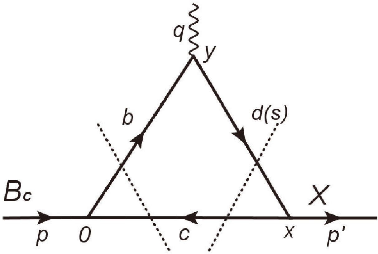
In the framework of QCDSR, the form factors are obtained by equating correlation functions on the phenomenological and QCD sides, where the correlation function is represented in hadronic and quark-gluon languages, respectively. Thus, the first step to obtain form factor is to write the following three-point correlation function:

where T is the time order operation. For the form factors of $ B_c \to D^{(*)} $ and $ B_c \to D_{s}^{(*)} $, X denotes the meson $ D^{(*)} $ or $ D_s^{(*)} $. p and $ p' $ are the momentums of $ B_c $ and $ D^{(*)}/D_s^{(*)} $ mesons, respectively, and$ J_{B_c} $ and $ J_X $ are interpolating currents that have the same quantum numbers as these mesons. $ J(y) $ is transition current, which is extracted from the low-energy effective Hamiltonian. These currents are written as follows:

where q in the last equation denotes d and s quark for form factors of $ B_c \to D^{(*)} $ and $ B_c \to D_s^{(*)} $, respectively. $ \Gamma = I, \gamma_\mu, \gamma_\mu \gamma_5, \sigma _{\mu \nu }\gamma_5 $, which correspond to scalar, vector, axial vector, and tensor form factors, respectively.

On the phenomenological side, a complete set of hadronic states with same quantum numbers as the current operators $ J_{B_c} $ and $ J_X $ are inserted into the correlation function. After the ground state contributions are isolated, the correlation functions can be expressed as

where $ h.r. $ denotes the contributions of excited and continuum states. The meson transition matrix elements are parameterized by various form factors:

where $ q = p-p' $, P denotes the pesudoscalar meson D or $ D_s $, V represents the vector meson $ D^* $or $ D_s^* $, ξ is the polarization vector of the relevant vector meson. Form factors at the maximally recoil point ($ q^{2} = 0 $) satisfy the following relations [40]:

The meson vacuum matrix elements in Eq. (3) can be parameterized as decay constants,

where $ m_{1} $ and $ m_{2} $ are the masses of quarks constituting the pesudoscalar meson. Replacing matrix elements in Eq. (3) with the expressions of Eqs. (4) and (6), we can expand the correlation function into different tensor structures. Taking the vector form factors of the $ B_c \to D $ transition as an example,

with

On the QCD side, the correlation function will have the same tensor structures as those on the phenomenological side. After equating both of these sides with the same tensor structure, the form factors $ f_+ $ and $ f_0 $ can be expressed as a linear combination of invariant amplitudes of the tensor structures $ p_\mu $ and $ p'_\mu $. We can also obtain the other form factors according to similar processes.

At the quark level, the quark fields in the correlation function expressed in Eq. (1) are contracted using Wick's theorem. Thus, the correlation functions on the QCD side for $ B_c \to D $, $ B_c \to D^* $, $ B_c \to D_s $, and $ B_c \to D_s^* $ processes can be expressed as

where $ D^{ij} $, $ S^{ij} $, $ C^{ij} $, and $ B^{ij} $ are the full propagators of d, s, c, and b quarks, respectively. These propagators can be written as follows [41]:

where $ q^{ij} $ and $ Q^{ij} $ denote light and heavy quark full propagators, respectively, i and j are color indices, ${\sigma _{\alpha \beta }} = {\rm i} [{\gamma _\alpha },{\gamma _\beta }]/2$, ${D_\alpha } = {\partial _\alpha } - {\rm i}{g_s}G_\alpha ^n{t^n}$, $ G_\alpha^n $ is the gluon field, $ {t^n} = {\lambda ^n}/2 $, and $ {\lambda ^n} $ is the Gell-Mann matrix. $ {f^{\lambda \alpha \beta }} $ and $ {f^{\alpha \beta \mu \nu }} $ are defined as

Performing the operator product expansion (OPE), the correlation functions are represented in different tensor structures on the QCD side, the same as those on the phenomenological side. Taking the vector form factor $ B_c \to D $ as an example, its correlation function is written in the following form:

Here, $ F_i(q^2) $ is called invariant amplitude, which is a function of transfer momentum squared. For each Dirac structure, the invariant amplitude can be expressed as the spectra density $ \rho(s,u,q^2) $ according to the dispersion integral

where $ s_{min} $ and $ u_{\min} $ are kinematic limits with values $ s_{\min} = (m_c+m_b)^2 $ and $ u_{\min} = (m_{d(s)}+m_c)^2 $. $ \rho_i(s,u,q^2) $ is the QCD spectral density, where $ s = p^2 $, $ u = p'^2 $. The spectral density is obtained from the imaginary part of the correlation function, and it originates from the contributions of perturbative and non-perturbative parts.

According to Cutkosky's rule [42, 43], the spectral density of the perturbative part can be obtained by putting all quark lines on shell (Fig. 1). In this process, the following condition should be satisfied:

Figure 1.  Feynman diagram for the perturbative part. The dashed lines denote the Cutkosky’s cuts.

where the λ function has following expression:

The non-perturbative contribution is reflected in several vacuum condensates, including the quark condensate, two-gluon condensate, quark-gluon mixing condensate, and three-gluon condensate. These vacuum condensates are illustrated in Fig. 2. After lengthy and complex derivation, we find that the contributions from quark condensate and quark-gluon mixing condensate only depend on $ p'^2 $ and $ q^2 $. Thus, these contributions are zero after performing the double Borel transformation with respect to both $ p^2 $ and $ p'^2 $. The spectral densities of gluon condensates can be obtained by a similar procedure as that of the perturbative part. To obtain its spectral density by Cutkosky's rule, the following equation is used to reduce the power of the quark propagator:

Figure 2.  Feynman diagrams of vacuum condensates. Contributions from quark condensate (q) and quark-gluon mixing condensates (r)-(x) are zero in the calculation.

After the spectral densities have been calculated, the sum rules for form factors can be obtained by matching the phenomenological and QCD sides. To eliminate the contributions from excited and continuum states, the threshold parameters $ s_{0} $ and $ u_{0} $are introduced, and the double Borel transformation is performed to enhance the contribution of the ground state while suppressing those of the excited and continuum states. Taking the vector form factors of the $ B_c \to D $ transition as an example, the sum rules can be expressed as

where substitutions of $ p^{2}\rightarrow -P^{2} $, $ p'^{2}\rightarrow -P'^{2} $, and $ q^{2}\rightarrow -Q^{2} $ are conducted, and the threshold parameters $ s_0 $ and $ u_0 $ serve as the upper limits of the integral. After performing double Borel transformation with respect to $ P^{2} $ and $ P'^{2} $, there are two Borel parameters $ M^2 $ and $ M'^2 $. Physical properties extracted from sum rules should be as independent of Borel parameters as possible. Because of the weak dependence, we can take $ M^{\prime2} = kM^2 $ with the factor $ k = m_{X}^2/m_{B_c}^2 $[44].

With respect to three-point QCD sum rules, the accurate calculation of the perturbative $ {\cal{O}}(\alpha_s) $correction is highly complex and not available currently. It is shown that the upper limits of integral are $ s_0 $ and $ u_0 $ in Eq. (20). In these integral regions, the relative velocity of component quarks in heavy quarkonia $ B_c $ is small. Under this condition, the expansion of perturbative correction can be executed in parameter $ \alpha_s/v $ rather than $ \alpha_s $[12], where v represents the relative velocity of component quarks in $ B_c $. The $ \alpha_s/v $ correction originating from Coulomb-like interaction of quarks is represented in Fig. 3. Ref. [12] proposed an approximate solution to this problem based on nonrelatistic potential, which is realized by multiplying the leading order spectral density by a renormalization coefficient $ {\cal{C}} $. In some other similar studies performed using two- or three-point QCDSR [45, 46], it was indicated that this Coulomb-like correction can lead to remarkable enhancement of spectral density numerically. In the present study, we employ the same method as in Ref. [12] and present bare form factors without considering Coulomb-like correction and modified form factors with correction. Certainly, it will be interesting and significant to perform straightforward calculations of perturbative correction, which can further improve the reliability of the final results. The modified spectral density of the perturbative term is as follows:

Figure 3.  Ladder Feynman diagram of the Coulomb-like correction.

where v is the relative velocity of quarks in the $ B_c $ meson:

The masses of mesons used in this study are taken from the Particle Date Group (PDG) [47]. The masses of quarks are energy-scale dependent and can be expressed by the following renormalization group equation:

where $t = \log ({\mu ^2}/{\Lambda _{\rm QCD}^2})$, $ {b_0} = ({33 - 2 n_f})/{12\pi} $, $ {b_1} = (153 - 19 n_f)/{24 \pi^2} $, and $ {b_2} = \left({2857 - \dfrac{5033}{9}{n_f} + \dfrac{325}{27}n_f^2}\right)/{128 \pi^3} $. The $ \overline{\mathrm{MS}} $ masses are also taken from the PDG with $ m_{c}(m_{c}) = 1.275\pm0.025 $ GeV and $ m_{b}(m_{b}) = 4.18\pm0.03 $ GeV. $ \Lambda _{QCD} = 213 $ MeV for the flavors $ n_f = 5 $ and the energy-scales are uniformly determined to be $ 2 $GeV, which were also adopted in our previous study [39]. The decay constants of mesons are taken from Refs. [48] and [49], where these hadronic parameters are uniformly obtained by QCDSR. The vacuum condensates are taken as standard values from Refs. [50−52]. Threshold parameters $ s_0 $ and $ u_0 $ are used to eliminate the contributions of excited and continuum states. Generally, their values are taken to be $ s_0 = (m_{B_c}+\Delta)^2 $ and $ u_0 = (m_X+\Delta)^2 $, where X represents the final meson $ D^{(*)} $ or $ D_s^{(*)} $. Theoretically, the value of ∆ should be larger than the width of the ground state and be smaller than the distance between the ground state and first excitation. In this study, ∆ is chosen to be $ 0.4 $, $ 0.5 $, and $ 0.6 $GeV for the lowest, central, and highest values of form factors. All of the values of parameters used in this study are listed in Table 1.

Parameters	Values/GeV	Parameters	Values
$ m_{B_c} $	6.27	$ f_{B_c} $	0.371 GeV [48]
$ m_{D} $	1.87	$ f_{D} $	0.208 GeV [49]
$ m_{D^*} $	2.01	$ f_{D^*} $	0.263 GeV [49]
$ m_{D_s} $	1.97	$ f_{D_s} $	0.240 GeV [49]
$ m_{D^*_s} $	2.11	$ f_{D^*_s} $	0.308 GeV [49]
$ m_{\eta_c} $	2.98	$ f_{\eta_c} $	0.387 GeV [53]
$ m_{J/\psi} $	3.10	$ f_{J/\psi} $	0.418 GeV [53]
$m_s(2\; \mathrm{GeV})$	0.095	$ \left\langle {g_s^2{G^2}} \right\rangle $	$ (0.88 \pm 0.15) $ GeV$ ^4 $
$m_c(2\;\mathrm{GeV})$	1.16	$ \left\langle {g^3f_{abc}{G^3}} \right\rangle $	$ (8.8 \pm 5.5) $ GeV$ ^2 \left\langle {\alpha_s{G^2}} \right\rangle $
$m_b(2\;\mathrm{GeV})$	4.76	$ V_{cb} $	0.041 [47]
$ V_{cd} $	0.221 [47]	$ V_{cs} $	0.975 [47]
$ a_1 $	1.07 [23]	$ a_2 $	0.234 [23]

Table 1.  Values of parameters used in this study; the values with no reference are mentioned in the text.

The Borel parameter $ M^2 $ is determined according to two conditions: pole dominance ($ \geq40$%) and convergence of OPE. The pole contribution is defined as follows [44]:

with

Still taking the vector form factor of $ B_c \to D $ as an example, we introduce how the Borel parameters are determined. Fixing $ Q^2 = 1 $ GeV$ ^2 $, we plot the variation of pole contribution with Borel parameter $ M^2 $ in Fig. 4. It is shown that the pole contribution decreases with increasing Borel parameter $ M^2 $. When the Borel parameter is smaller than $ 28 $ GeV$ ^2 $, the pole contribution is above $ 40$%. To find the Borel platform where the condition of OPE convergence is satisfied and the results have good stability and convergence, the contributions of the perturbative part and all vacuum condensate terms are plotted in Fig. 5. It is clear that the contribution of the perturbative term is dominant in the region $ 23\;{\rm GeV^2} \leq $ $ M^2\leq27 $ GeV², while the contributions from vacuum condensate terms are much less. That is, the OPE convergence is well satisfied. According to the above analyses, the Borel platform is determined to be $ 23 $$ -27 $ GeV², where the conditions of the pole dominance ($ \geq40$%) and convergence of OPE are all satisfied. The values of Borel parameters and pole contributions for different form factors are all listed in Table 2.

Figure 4.  (color online) Pole contributions of vector form factors of $ B_c \to D $ transition. (a) and (b) correspond to $ f_+^{B_c \to D} $ and $ f_0^{B_c \to D} $, respectively.

Figure 5.  (color online) Contributions of the perturbative part and different vacuum condensate terms with variation of the Borel parameter.

Modes	Form factors	Borel platforms	Pole contributions(%)
$ B_c \to D $	$ f_s $	20 $ \sim $ 24	51.27
	$ f_+ $	23 $ \sim $ 27	50.20
	$ f_0 $	23 $ \sim $ 27	50.95
	$ f_T $	30 $ \sim $ 34	50.02
$ B_c \to D^* $	V	33 $ \sim $ 37	50.12
	$ A_0 $	25 $ \sim $ 29	51.78
	$ A_1 $	22 $ \sim $ 26	50.48
	$ A_2 $	19 $ \sim $ 23	51.34
$ B_c \to D_s $	$ f_s $	21 $ \sim $ 25	51.58
	$ f_+ $	24 $ \sim $ 28	50.91
	$ f_0 $	24 $ \sim $ 28	51.65
	$ f_T $	31 $ \sim $ 35	50.70
$ B_c \to D_s^* $	V	33 $ \sim $ 37	51.03
	$ A_0 $	26 $ \sim $ 30	50.91
	$ A_1 $	22 $ \sim $ 26	52.59
	$ A_2 $	20 $ \sim $ 24	50.13

Table 2.  Borel platform and pole contribution for different form factors.

After all of these parameters are determined, the form factors in the space-like region ($ Q^2 = -q^2>0 $) are calculated. Then, these values are fitted into an appropriate analytical function, which is used to extrapolate the form factor into the time-like region ($ Q^2 = -q^2<0 $). In this study, the $ z $-series parameterization approach is employed to realize this process. For vector, axial vector, and tensor form factors, the following parameterized function is adopted [54, 55]:

The scalar form factor is fitted in another form:

where $ m_R $ is the mass of low-lying $ B_c $ resonance [56], and $ z(Q^2,t_0) $ is written as

Here, $ t_0 $ is a free parameter in the region (-$ \infty $, $ t_+ $), which can be used to optimize the convergence of the series expansion. In the present study, the auxiliary parameter $ t_0 $ is taken as [54, 56, 57]

where $ t_\pm = (m_{B_c}\pm m_X)^2 $. The expansion coefficients $ b_i $ in Eqs. (26) and (27) are obtained by fitting the numerical results with these two equations in the space-like region. All of the fitting parameters are listed in Table 3, and the fitting diagrams are shown in Fig. 6. It can be seen that all of the numerical results are well fitted by the these fitting functions. Thus, we can obtain the values of form factors at $ Q^2 = 0 $ with these fitting functions. The results obtained in this study, together with those of other collaborations, are summarized in Table 4.

Modes	Form factors	$ b_0 $	$ b_1 $	$ b_2 $
$ B_c \to D $	$ f_s $	0.54	-5.9	14
	$ f_+ $	0.093	-1.4	5.5
	$ f_0 $	0.073	-0.78	1.6
	$ f_T $	0.032	-0.45	1.6
$ B_c \to D^* $	V	0.28	-3.7	13
	$ A_0 $	0.20	-3.1	13
	$ A_1 $	0.12	-1.0	1.3
	$ A_2 $	0.082	-0.56	-1.0
$ B_c \to D_s $	$ f_s $	0.65	-6.5	13
	$ f_+ $	0.11	-1.6	6.2
	$ f_0 $	0.087	-0.85	1.6
	$ f_T $	0.037	-0.50	1.8
$ B_c \to D_s^* $	V	0.29	-3.8	13
	$ A_0 $	0.21	-3.2	13
	$ A_1 $	0.13	-1.1	1.2
	$ A_2 $	0.095	-0.61	-1.3

Table 3.  Fitting parameters of the z-series parameterized approach.

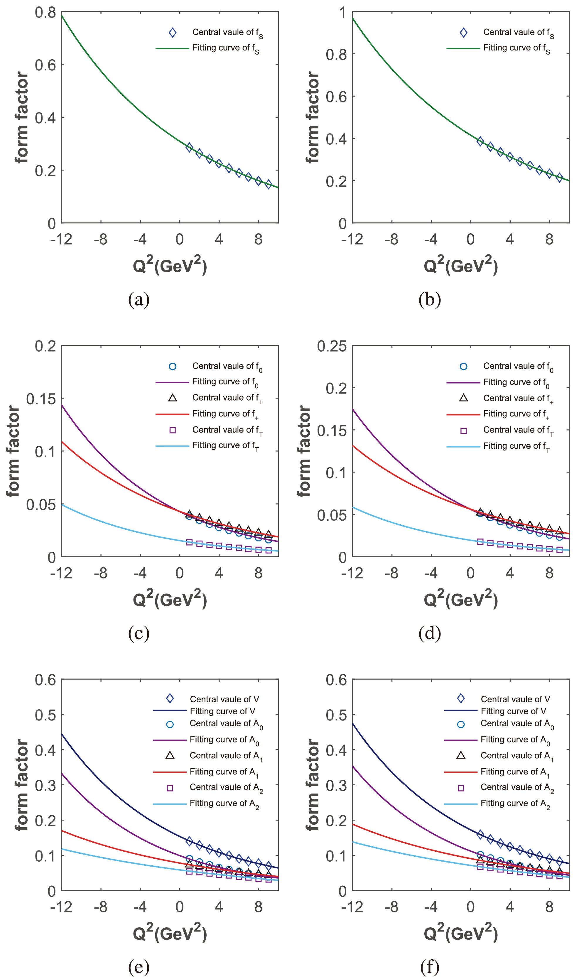
Figure 6.  (color online) Fitting diagrams of form factors. (a), (c), and (e) show the fitting results of form factors $ B_c \to D^{(*)} $ transition, while (b), (d), and (f) show those of $ B_c \to D_s^{(*)} $.

Modes	Form factors	This study	This study*	[19]	[20]	[23]	[15, 16]
$ B_c \to D $	$ f_S $	$ 0.31^{+0.10}_{-0.10} $	$ 0.54^{+0.18}_{-0.17} $	−	−	−	−
	$ f_+ $	$ 0.043^{+0.014}_{-0.014} $	$ 0.076^{+0.026}_{-0.024} $	0.075	0.16	$ 0.17^{+0.01}_{-0.01} $	0.22
	$ f_0 $	$ 0.043^{+0.014}_{-0.014} $	$ 0.077^{+0.026}_{-0.024} $	0.075	0.16	$ 0.17^{+0.01}_{-0.01} $	0.22
	$ f_T $	$ 0.015^{+0.005}_{-0.005} $	$ 0.027^{+0.009}_{-0.009} $	−	−	−	−
$ B_c \to D^* $	V	$ 0.15^{+0.04}_{-0.04} $	$ 0.28^{+0.08}_{-0.08} $	0.16	0.13	$ 0.20^{+0.03}_{-0.03} $	0.63
	$ A_0 $	$ 0.099^{+0.028}_{-0.027} $	$ 0.18^{+0.05}_{-0.05} $	0.081	0.09	$ 0.14^{+0.02}_{-0.02} $	0.34
	$ A_1 $	$ 0.078^{+0.022}_{-0.021} $	$ 0.14^{+0.04}_{-0.04} $	0.095	0.08	$ 0.13^{+0.02}_{-0.02} $	0.41
	$ A_2 $	$ 0.059^{+0.016}_{-0.016} $	$ 0.10^{+0.03}_{+0.03} $	0.11	0.07	$ 0.12^{+0.01}_{-0.01} $	0.45
$ B_c \to D_s $	$ f_S $	$ 0.41^{+0.12}_{-0.12} $	$ 0.73^{+0.21}_{-0.20} $	−	−	−	−
	$ f_+ $	$ 0.056^{+0.016}_{-0.016} $	$ 0.10^{+0.03}_{-0.03} $	0.15	0.28	$ 0.21^{+0.01}_{-0.01} $	0.16
	$ f_0 $	$ 0.056^{+0.016}_{-0.016} $	$ 0.10^{+0.03}_{-0.03} $	0.15	0.28	$ 0.21^{+0.01}_{-0.01} $	0.16
	$ f_T $	$ 0.020^{+0.006}_{-0.006} $	$ 0.035^{+0.011}_{-0.010} $	−	−	−	−
$ B_c \to D_s^* $	V	$ 0.17^{+0.04}_{-0.04} $	$ 0.32^{+0.08}_{-0.08} $	0.29	0.23	$ 0.25^{+0}_{-0} $	0.54
	$ A_0 $	$ 0.11^{+0.03}_{-0.03} $	$ 0.20^{+0.05}_{-0.05} $	0.16	0.17	$ 0.18^{+0.02}_{-0.03} $	0.30
	$ A_1 $	$ 0.091^{+0.023}_{-0.022} $	$ 0.16^{+0.04}_{-0.04} $	0.18	0.14	$ 0.16^{+0.01}_{-0.02} $	0.36
	$ A_2 $	$ 0.072^{+0.018}_{-0.017} $	$ 0.13^{+0.03}_{-0.03} $	0.20	0.12	$ 0.15^{+0.01}_{-0.01} $	0.24

Table 4.  Numerical results of the form factors $ B_c \to D^{(*)} $ and $ B_c \to D_{s}^{(*)} $ at $ Q^2=0 $; the values in the fourth column denote the results with Coulomb-like correction.

It is shown that form factors are inconsistent across different studies. Our predictions for $ f_+ $ and $ f_0 $ are small compared to those of other studies, but for axial vector form factors $ A_{0,1,2} $, the numerical results predicted in this study are roughly in agreement with those in Refs. [19, 20, 23], where the BSW, CLFQM, and CLFQM methods were adopted. In Ref. [16], the authors also adopted three-point QCDSR to carry out a similar analysis; however, their results are much larger than ours. Unfortunately, we failed to reconstruct their results using the spectral density shown in Ref. [16]. Besides, it is shown that form factors of the $ B_c \to D_s $ transition are larger than those of the $ B_c \to D $ process. This characteristic is consistent with the predictions in Refs. [19, 20, 23], but the results in Refs. [15, 16] show a completely opposite trend. From Table 4, we can also see that the numerical results of form factors are approximately twice that of the bare form factors after considering the Coulomb-like correction. After performing this correction, the values of $ f_+ $ and $ f_0 $ are compatible with the results of BSW [19]. Although there are some differences between the numerical results obtained by different methods, these results exhibit similar characteristics. For example, the vector form factor V is larger than the axial vector form factor $ A_{0,1,2} $. As for the form factors of $ B_c\to D $ and $ B_c\to D_{s} $, the value of $ f_{s} $ is evidently larger than those of the others.

In our previous study, the decay widths of several two-body decays for $ B_c $ to charmonium plus one light meson were predicted [39]. As a continuation, two-body decay processes of $ B_c $ to charmonium plus $ D^{(*)} $ or $ D_s^{(*)} $ mesons were analyzed in this study. This kind of decay process is realized according to weak decay of the b-quark with the c-quark acting as a spectator, as illustrated in Fig. 7. The effective Hamiltonian for this process has the following form:

Figure 7.  (color online) Feynman diagram of $ B_c $ decaying to charmonium plus X meson (X = $ D^{*} $, $ D_s^{*} $,D, $ D_s $). The solid lines of red, green, and blue represent propagators of $ d/s $, c, and b quarks, respectively.

where $G_{\rm F}$ is the Fermi constant, $ V_{cb} $ and $ V_{cq}^* $ are the CKM matrix elements, q denotes the d or s quark, and $ a_1 $ and $ a_2 $ are Wilson coefficients. $ O_1 $ and $ O_2 $ are four-fermion operators, which are defined as

The decay width of the two-body decay process can be expressed as

where $ {\bf{p}} $ is the three-momentum of either of the final particles in the $ B_c $ rest frame:

where $ m_1 $ and $ m_2 $ are the masses of two daughter particles. In the framework of the factorization approach, the matrix element T in Eq. (32) can be decomposed as the production of two matrix elements [58]:

with X = D, $ D^{*} $, $ D_s $, $ D_s^{*} $ and C = $ \eta_{c} $, $ J/\psi $. The meson transition matrix elements at the right side of Eq. (34) have been parameterized as various form factors in Eq. (4), and meson vacuum matrix elements can be parameterized as the following decay constants:

with P denoting the$ D_{s} $, D, or $ \eta_{c} $ meson and V representing the $ D_{s}^{*} $, $ D^{*} $, or $ J/\psi $ meson. The values of form factors $ B_{c}\to X $ have been determined in Sec. III, and those of $ B_{c}\to C $ are taken from our previous study [39]. All of the values of parameters used in this section are also listed in Table 1. With these above equations, the decay widths of these decay processes can be written as

where $ A_{0}, A_{+}, A_{-} $ are three polarization amplitudes and can be written as

The numerical results of the decay widths and branching ratios are all listed in Table 5. It can be seen that the decay widths and branching ratios with Coulomb-like correction increase by approximately 9 times compared with the results without correction. In most of the literature, only the branching ratios were listed. It is shown that these branching ratios from different studies are located in a broad range. In the present study, the branching ratios obtained with bare form factors are smaller than most of the other results. This is mainly due to the smaller values of predicted form factors, which will contribute to square reduction in the values of decay widths. If Coulomb-like correction is considered, the branching ratios are compatible with most of the other predictions. Furthermore, we can also see that the decay widths of $ B_{c}\to D_{s}^{(*)} $ are larger than those of $ B_{c}\to D^{(*)} $ processes. This is because the values of the CKM matrix elements $ V_{cs} $ are much larger than $ V_{cq} $ (see Table 1), and their form factors also have the same characteristic. For example, the values of $ f_{S} $ for the $ B_{c}\to D_{s} $ and $ B_{c}\to D $ processes are $ 0.41^{+0.12}_{-0.12} $ and $ 0.31^{+0.10}_{-0.10} $, respectively (see Table 4). Besides, the predicted branching ratios for most of the decay channels are in the range $ 10^{-5} $$ \sim $$ 10^{-3} $, which lies within the detected ability of LHCb experiment. Thus, all of these theoretical results can be verified by experiments in the near future. Finally, using the results of the decay process $ B_c \to J/\psi \pi $ from our previous study [39], we obtain the following ratios: $ \dfrac{B(B_c \to J/\psi D_s)}{B(B_c \to J/\psi \pi)} = 3.3^{+1.0}_{-0.9} $, $ \dfrac{B(B_c \to J/\psi D_s^*)}{B(B_c \to J/\psi D_s)} = 5.3^{+4.0}_{-2.2} $. The former is consistent with the experimental data $ 2.90 \pm 0.57 \pm 0.24 $, while the latter is larger than the experimental data $ 2.37 \pm 0.56 \pm 0.1 $ [6].

Decay channels	Decay widths ($ 10^{-7} $eV)			Branching ratios ($ 10^{-3} $)
	This study	This study$ ^* $		This study	This study$ ^* $	[60]	[61]	[62]	[13]	[63]	[23]	[64]
$ B_c^- \to D \eta_c $	$ 0.37^{+0.11}_{-0.11} $	$ 3.1^{+0.8}_{-0.8} $		$ 0.028^{+0.009}_{-0.009} $	$ 0.24^{+0.06}_{-0.07} $	0.012	0.05	0.06	0.15	0.19	$ 0.22^{+0.03}_{-0.01} $	$ 0.44^{+0.25}_{-0.18} $
$ B_c^- \to D J/\psi $	$ 0.46^{+0.13}_{-0.12} $	$ 3.9^{+0.9}_{-0.9} $		$ 0.036^{+0.010}_{-0.009} $	$ 0.30^{+0.07}_{-0.07} $	0.009	0.13	0.04	0.09	0.15	$ 0.20^{+0.03}_{-0.03} $	$ 0.28^{+0.12}_{-0.08} $
$ B_c^- \to D^* \eta_c $	$ 0.52^{+0.16}_{-0.16} $	$ 4.1^{+1.1}_{-1.1} $		$ 0.04^{+0.01}_{-0.01} $	$ 0.32^{+0.08}_{-0.09} $	0.010	0.02	0.07	0.10	0.19	$ 0.31^{+0.02}_{-0.02} $	$ 0.58^{+0.36}_{-0.25} $
$ B_c^- \to D^* J/\psi $	$ 2.2^{+0.6}_{-0.6} $	$ 18^{+4}_{-4} $		$ 0.17^{+0.05}_{-0.04} $	$ 1.4^{+0.3}_{-0.3} $	-	0.19	-	0.28	0.45	$ 0.41^{+0.06}_{-0.02} $	$ 0.67^{+0.31}_{-0.19} $
$ B_c^- \to D_s \eta_c $	$ 9.6^{+2.8}_{-2.9} $	$ 82^{+20}_{-22} $		$ 0.74^{+0.22}_{-0.23} $	$ 6.4^{+1.6}_{-1.7} $	0.54	5	1.79	2.8	4.4	$ 6.44^{+1.78}_{-1.32} $	$ 12.32^{+7.20}_{-5.56} $
$ B_c^- \to D_s J/\psi $	$ 11^{+3}_{-3} $	$ 97^{+23}_{-22} $		$ 0.89^{+0.25}_{-0.23} $	$ 7.5^{+1.8}_{-1.5} $	0.41	3.4	1.15	1.7	3.4	$ 6.09^{+1.62}_{-0.91} $	$ 8.05^{+3.62}_{-2.08} $
$ B_c^- \to D_s^* \eta_c $	$ 13^{+4}_{-4} $	$ 103^{+25}_{-27} $		$ 1.0^{+0.3}_{-0.3} $	$ 8.0^{+1.9}_{-2.1} $	0.44	0.38	1.49	2.7	3.7	$ 6.97^{+0.68}_{-0.33} $	$ 16.54^{+10.08}_{-8.74} $
$ B_c^- \to D_s^* J/\psi $	$ 58^{+16}_{-15} $	$ 488^{+112}_{-108} $		$ 4.6^{+1.2}_{-1.1} $	$ 38^{+9}_{-8} $	-	5.9	-	6.7	9.7	$ 9.03^{+0.40}_{-0.38} $	$ 20.45^{+10.24}_{-8.44} $

Table 5.  Decay widths and branching ratios of $ B_c $ decaying to charmonium. The results in the third and fifth columns are obtained considering the Coulomb-like correction. Branching ratios are calculated at $ \tau_{B_c} $ = 0.51 ps [59].

It should be noted that predictions of nonleptonic decays with the naive factorization approach suffer from systematic uncertainties. This is because this method neglects the strong interaction between the meson emitted from the weak vertex and the transition form factor, which leads to non-factorizable correction. One can improve the accuracy by invoking several developed methods, including the pQCD and QCD factorization (QCDF). These techniques have been widely used to study the nonleptonic decays of B mesons [65−70]. For more details about the factorization methods, one can consult the above literature.

In this study, the form factors for $ B_c \to D^{(*)} $ and $ B_c \to D_s^{(*)} $ transition processes are systematically analyzed in the framework of three-point QCDSR. The numerical results in the space-like region ($ Q^2 = -q^2 > 0 $) are first calculated and then fitted into analytical functions using the $ z- $series parameterizations approach. With these analytical functions, we obtain the form factors at $ Q^2 = 0 $ and $ Q^2 = - M^2 $ by extrapolating the results into the time-like region ($ Q^2 = -q^2 < 0 $). Using these form factors, the decay widths and branching ratios of two-body nonleptonic decays including $ B_c \to \eta_c D^{*} $, $ \eta_c D $, $ J/\psi D^{*} $, $ J/\psi D $, $ \eta_c D_s^{*} $, $ \eta_c D_s $, $ J/\psi D_s^{*} $, and $ J/\psi D_s $are obtained with the factorization method. All of the results on form factors, decay widths, and branching ratios obtained in this study provide useful information for further studying heavy-quark dynamics and may also be helpful in future experiments of heavy flavor physics.