


 Abstract
 HTML
 Reference
 Related
 PDF

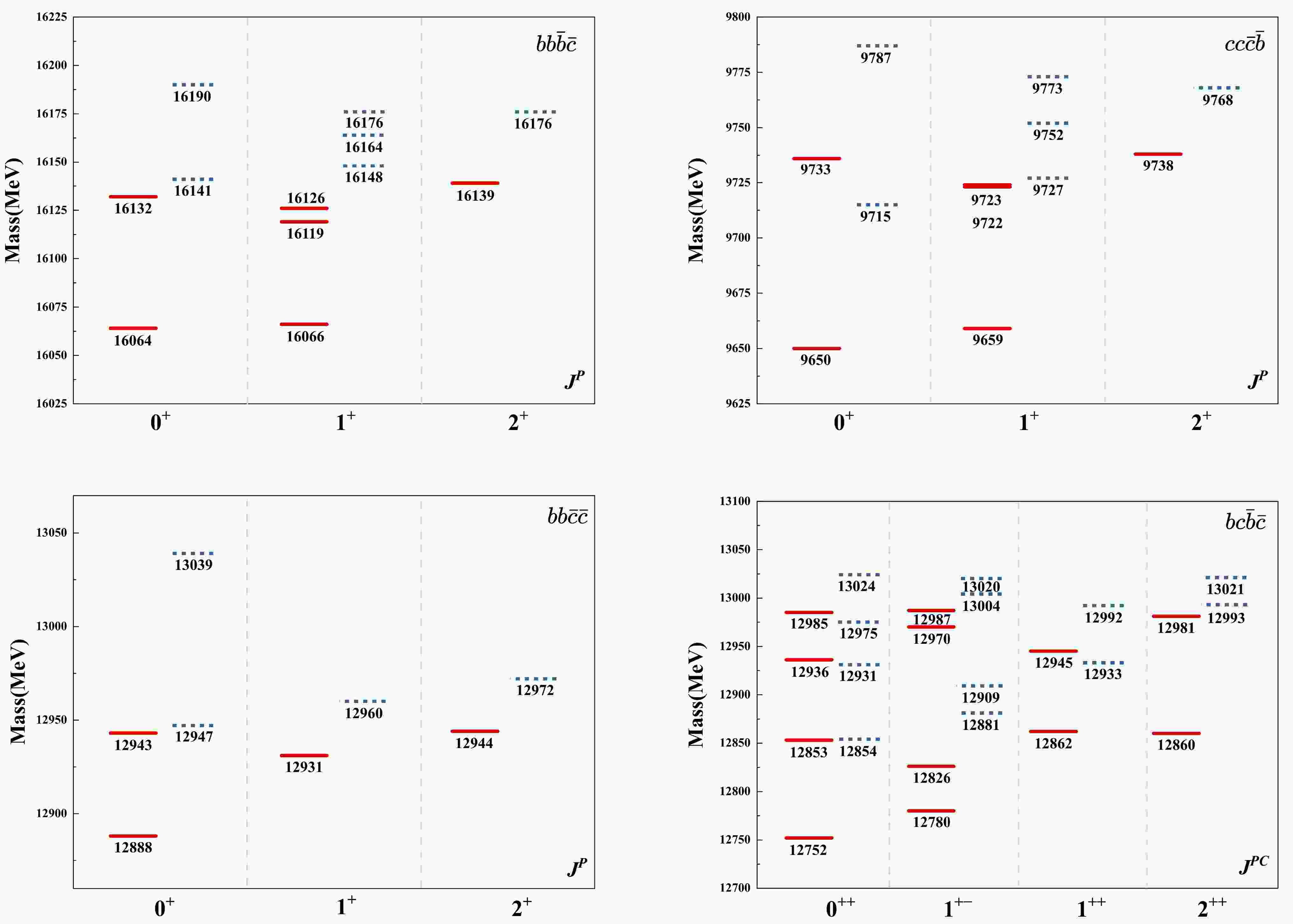


-
Among exotic hadrons, the all-heavy tetraquarks have attracted considerable attention as systems of significant interest. Since light mesons cannot be exchanged, all-heavy tetraquarks are considered ideal systems for exploring genuine compact tetraquark states. In 2020, the LHCb collaboration observed a narrow structure
$ X(6900) $ in the di-$ J/\psi $ invariant mass spectrum [1]. Its existence was later confirmed independently by the CMS [2] and ATLAS [3] collaborations. Furthermore, the CMS also observed two additional structures$ X(6600) $ and$ X(7100) $ in the di-$ J/\psi $ invariant mass spectrum [2]. These structures could be interpreted as tetraquark states with four charm quarks,$ cc\bar{c}\bar{c} $ [4−12]. The CMS and LHCb collaborations have also searched for the fully bottomed tetraquarks$ bb\bar{b}\bar{b} $ ; however, no significant signals have been found so far [13−15].In addition to
$ cc\bar{c}\bar{c} $ and$ bb\bar{b}\bar{b} $ , there exist other all-heavy tetraquarks containing both charm and bottom quarks:$ bb\bar{b}\bar{c} $ /$ bc\bar{b}\bar{b} $ ,$ cc\bar{c}\bar{b} $ /$ bc\bar{c}\bar{c} $ ,$ bb\bar{c}\bar{c} $ /$ cc\bar{b}\bar{b} $ , and$ bc\bar{b}\bar{c} $ . The recent discovery of several$ cc\bar{c}\bar{c} $ candidates at the LHC indicates that experimental investigation of other all-heavy tetraquark states containing both charm and bottom quarks also has considerable potential. In fact, the LHC has also demonstrated a powerful capability for searching for hadrons containing both charm and bottom quarks. For example, several excited$ B_c $ states [16−18] and evidence of the doubly heavy baryon$ \Xi_{bc} $ [19] were recently observed at the LHC. This experimental progress has stimulated theoretical interest in these all-heavy tetraquarks with different flavors. In recent years, numerous studies of the mass spectra have been performed using various models and approaches, such as various nonrelativistic constituent quark models [9, 10, 20−26], diquark models [11, 27−31], QCD sum rules [32−48], color-magnetic models [7, 22, 49, 50], the Bethe-Salpeter equation method [51], the flux-tube model [22], the bosonic algebraic approach [52], a conditional generative adversarial network (CGAN) [53], the pNRQCD method [54], the heavy meson exchange model [55], among others. However, a comparison of existing model calculations reveals strong model dependence in the results.For the all-heavy tetraquark systems with different flavors, namely
$ bb\bar{b}\bar{c} $ /$ bc\bar{b}\bar{b} $ ,$ cc\bar{c}\bar{b} $ /$ bc\bar{c}\bar{c} $ , and$ bb\bar{c}\bar{c} $ /$ cc\bar{b}\bar{b} $ , the$ 1S $ -wave mass spectra were preliminarily studied using a nonrelativistic quark potential model by our group in 2019 [9]. In these calculations, the oscillator parameter of the trial wave function was approximately treated as being independent of the quark mass when solving for the mass spectrum via the variational method. However, such a treatment would lead to substantial incompleteness in the trial wave function for all-heavy tetraquark systems with different quark flavors. In the present work, to improve the completeness of the trial wave function and obtain more reliable predictions of the mass spectra, we revisit the$ bb\bar{b}\bar{c} $ /$ bc\bar{b}\bar{b} $ ,$ cc\bar{c}\bar{b} $ /$ bc\bar{c}\bar{c} $ , and$ bb\bar{c}\bar{c} $ /$ cc\bar{b}\bar{b} $ systems by adopting correlated Gaussian functions [56−58] as the radial wave function basis. This method is known to be effective and accurate for solving few-body problems.Because the obtained
$ 1S $ -wave all-heavy tetraquark states with different flavors lie far above the threshold for dissociation into two ground-state mesons, we further evaluate their fall-apart decay properties using a quark-exchange model [59, 60]. The present study on the fall-apart decay properties of the$ bb\bar{b}\bar{c} $ ,$ cc\bar{c}\bar{b} $ ,$ bb\bar{c}\bar{c} $ , and$ bc\bar{b}\bar{c} $ systems is a continuation of our previous work on the$ cc\bar{c}\bar{c} $ and$ bb\bar{b}\bar{b} $ systems [61]. By studying their decay properties, we expect to provide useful decay channels for future experimental observation. The decay properties of all-heavy tetraquark states with different flavors remain relatively unexplored. Only a few research groups have explored this issue using various methods, such as the complex scaling method [25], the real scaling method [24], the coupled-channels method [26], the CGAN framework [53], QCD sum rules [35−48], among others. The decay properties exhibit strong model dependence. For example, the tetraquarks$ bb\bar{b}\bar{c} $ and$ cc\bar{c}\bar{b} $ are predicted to be broad structures with a width of$ \sim100 $ MeV by QCD sum rules [42, 46−48], whereas the real scaling method predicts narrow structures with a width of about several MeV [24].This paper is organized as follows. In Sec. II, the theoretical framework is briefly introduced. In Sec. III, the numerical results and discussion for all-heavy tetraquarks with different flavors are presented. Finally, a brief summary is given in Sec. IV.
-
In this work, to describe the tetraquark system, we adopt a nonrelativistic Hamiltonian [9], i.e.,
$ H = \sum\limits_{i=1}^{4}\left(m_i +T_i\right)-T_G+\sum\limits_{i<j}V_{ij}(r_{ij}), $
(1) where
$ m_i $ and$ T_i $ denote the mass and kinetic energy of the i-th quark, respectively.$ T_G $ denotes the center-of-mass kinetic energy.$ V_{ij}(r_{ij}) $ represents the effective potential between the i-th and j-th quarks at a distance$ r_{ij}\equiv|\boldsymbol{r}_i-\boldsymbol{r}_j| $ . In this work, we adopt a widely used form for the potential$ V_{ij}(r_{ij}) $ [62−64], i.e.,$ \begin{aligned}[b] V_{ij}(r_{ij}) =\;& -\frac{3}{16}( {\boldsymbol{\lambda}}_i\cdot {\boldsymbol{\lambda}}_j)\left\{br_{ij}-\frac{4}{3}\frac{\alpha_{ij}}{r_{ij}}\right.\\& \left.+\alpha_{ij}\cdot\frac{\sigma^3_{ij}e^{-\sigma^2_{ij}r^2_{ij}}}{\pi^{1/2}}\cdot\frac{8}{9m_im_j}( {\boldsymbol{\sigma}}_i\cdot {\boldsymbol{\sigma}}_j)\right\}, \end{aligned} $
(2) where the first, second, and third terms correspond to the linear confinement part
$ V^{\mathrm{Conf}} $ , the color-Coulomb part$ V^{\mathrm{Coul}} $ , and the chromo-magnetic (spin-spin) part$ V^{\mathrm{SS}} $ , respectively.$ {\boldsymbol{\lambda}}_i $ and$ {\boldsymbol{\sigma}}_i $ denote the spin and color operators of the i-th quark, respectively. Here, b is the slope parameter of the confinement potentials, while the$ \alpha_{ij} $ are the strong coupling constants.The nine parameters
$ m_{c/b} $ ,$ \alpha_{cc/bb/bc} $ ,$ \sigma_{cc/bb/bc} $ , and b have been determined by fitting the$ c\bar{c} $ ,$ b\bar{b} $ , and$ {b\bar{c}} $ spectra in our previous works [9, 65, 66]. The parameter set, along with the theoretical masses compared with the experimental data [67], is listed in Table 1.Quark model parameters $ m_c/m_b $ (GeV)1.483/4.852 $ \alpha_{cc}/\alpha_{bc}/\alpha_{bb} $ 0.5461/0.5021/0.4311 $ \sigma_{cc}/\sigma_{bc}/\sigma_{bb} $ (GeV)1.1384/1.3000/2.3200 b(GeV $ ^2 $ )0.1425 Mass spectrum Meson Theor. Exp. [67] Meson Theor. Exp. [67] $ J/\psi(1S) $ 3097 3097 $ B_{c}(2S)^{\pm} $ 6871 6871 $ \eta_{c}(1S) $ 2983 2984 $ \Upsilon\text{(1S)} $ 9460 9460 $ \psi(2S) $ 3679 3686 $ \eta_{b}(1S) $ 9390 9399 $ \eta_{c}(2S) $ 3635 3638 $ \Upsilon(2S) $ 10024 10023 $ \chi_{c0}(1P) $ 3415 3415 $ \eta_{b}(2S) $ 10005 9999 $ \chi_{c1}(1P) $ 3516 3511 $ h_{b}(1P) $ 9941 9899 $ \chi_{c2}(1P) $ 3552 3556 $ \chi_{b0}(1P) $ 9859 9859 $ h_{c}(1P) $ 3522 3525 $ \chi_{b1}(1P) $ 9933 9893 $ B_{c}^{+} $ 6271 6274 $ \chi_{b2}(1P) $ 9957 9912 Table 1. The quark model parameters are determined by fitting the meson mass spectra. The meson masses are given in MeV.
-
To calculate the spectroscopy of a
$ Q_1Q_2\bar{Q}_3\bar{Q}_4 $ system, we first construct the configurations in the product space of spatial$ \otimes $ flavor$ \otimes $ color$ \otimes $ spin. In the flavor space, the available configurations for all all-heavy tetraquark systems with different flavors are$ bb\bar{b}\bar{c} $ ,$ cc\bar{c}\bar{b} $ ,$ bb\bar{c}\bar{c} $ , and$ bc\bar{b}\bar{c} $ . This implies that the flavor wave function is symmetric under the exchange of two identical quarks (antiquarks). Note that three additional systems,$ bc\bar{b}\bar{b} $ ,$ bc\bar{c}\bar{c} $ , and$ cc\bar{b}\bar{b} $ , are not included, as they correspond to the antiparticles of$ bb\bar{b}\bar{c} $ ,$ cc\bar{c}\bar{b} $ , and$ bb\bar{c}\bar{c} $ , respectively.For a tetraquark system, six spin configurations (
$ \chi^{S_{12}S_{34}}_{SS_z} $ ) and two colorless configurations ($ |6_{12}\bar{6}_{34}\rangle_c $ and$ |\bar{3}_{12}3_{34}\rangle_c $ ) can be constructed in the spin and color spaces based on SU(2) and SU(3) group representation theory, respectively. Here,$ S_{12} $ stands for the spin quantum number of the diquark ($ Q_1Q_2 $ ), while$ S_{34} $ stands for that of the other antidiquark ($ \bar{Q}_3\bar{Q}_4 $ ). S is the total spin quantum number of the tetraquark system, while$ S_z $ stands for the third component of the total spin$ \boldsymbol{S} $ . The explicit forms of the six spin configurations and two colorless configurations can be found in Ref. [9].In the spatial space, the relative Jacobi coordinates in terms of the single-particle coordinates
$ \boldsymbol{r}_i $ ($ i=1,2,3,4 $ ) are defined by$ \begin{array}{l} \begin{pmatrix} {\boldsymbol{\xi}}_1 \\[2ex] {\boldsymbol{\xi}}_2 \\[2ex] {\boldsymbol{\xi}}_3 \\[2ex] \boldsymbol{R} \end{pmatrix} = \begin{pmatrix} 1 & -1 & 0 & 0 \\[1.5ex] 0 & 0 & 1 & -1 \\[1.5ex] \dfrac{m_1}{m_{12}} & \dfrac{m_2}{m_{12}} & -\dfrac{m_3}{m_{34}} & -\dfrac{m_4}{m_{34}} \\[2ex] \dfrac{m_1}{M} & \dfrac{m_2}{M} & \dfrac{m_3}{M} & \dfrac{m_4}{M} \end{pmatrix} \begin{pmatrix} \boldsymbol{r}_1 \\[2ex] \boldsymbol{r}_2 \\[2ex] \boldsymbol{r}_3 \\[2ex] \boldsymbol{r}_4 \end{pmatrix}, \end{array} $
(3) where
$ m_{ij}=m_i+m_j $ and$ M=\sum_{i=1}^4m_i $ . Using the above Jacobi coordinates, one can readily construct basis functions with well-defined symmetry under permutations of the identical (anti)quark pairs [68]. For the low-lying$ 1S $ states considered in this work, there is no excitation between identical (anti)quarks; therefore, the spatial wave functions are constructed to be symmetric under the exchange of the identical (anti)diquark. It should be noted that for the low-lying$ 1S $ states, the orbital angular momentum between non-identical (anti)quarks is not necessarily zero (the reason will be discussed in Sec. II(A3) below). Therefore, there is no constraint on the symmetry of the spatial wave function under the exchange of two non-identical (anti)quarks.Finally, taking the Pauli principle into account, the numbers of
$ 1S $ configurations are: 6 for both the$ bb\bar{b}\bar{c} $ and$ cc\bar{c}\bar{b} $ systems, 4 for$ bb\bar{c}\bar{c} $ , and 12 for$ bc\bar{b}\bar{c} $ . It should be pointed out that for the purely neutral$ bc\bar{b}\bar{c} $ system, each configuration must be an eigenstate of charge conjugation. All these$ 1S $ -wave configurations for the$ bb\bar{b}\bar{c} $ ,$ cc\bar{c}\bar{b} $ ,$ bb\bar{c}\bar{c} $ , and$ bc\bar{b}\bar{c} $ systems are listed in Table 2.System $ J^{P(C)} $ Configuration $ bb\bar{b}\bar{c} $ $ 0^{+} $ $ |(bb)^6_0\{\bar{b}\bar{c}\}^{\bar{6}}_0\rangle^0_0 $ $ |(bb)^{\bar{3}}_1\{\bar{b}\bar{c}\}^3_1\rangle^0_0 $ $ \cdot\cdot\cdot $ $ 1^{+} $ $ |(bb)^6_0\{\bar{b}\bar{c}\}^{\bar{6}}_1\rangle^0_1 $ $ |(bb)^{\bar{3}}_1\{\bar{b}\bar{c}\}^3_1\rangle^0_1 $ $ |(bb)^{\bar{3}}_1\{\bar{b}\bar{c}\}^3_0\rangle^0_1 $ $ 2^{+} $ $ |(bb)^{\bar{3}}_1\{\bar{b}\bar{c}\}^3_1\rangle^0_2 $ $ \cdot\cdot\cdot $ $ \cdot\cdot\cdot $ $ cc\bar{c}\bar{b} $ $ 0^{+} $ $ |(cc)^6_0\{\bar{c}\bar{b}\}^{\bar{6}}_0\rangle^0_0 $ $ |(cc)^{\bar{3}}_1\{\bar{c}\bar{b}\}^3_1\rangle^0_0 $ $ \cdot\cdot\cdot $ $ 1^{+} $ $ |(cc)^6_0\{\bar{c}\bar{b}\}^{\bar{6}}_1\rangle^0_1 $ $ |(cc)^{\bar{3}}_1\{\bar{c}\bar{b}\}^3_1\rangle^0_1 $ $ |(cc)^{\bar{3}}_1\{\bar{c}\bar{b}\}^3_0\rangle^0_1 $ $ 2^{+} $ $ |(cc)^{\bar{3}}_1\{\bar{c}\bar{b}\}^3_1\rangle^0_2 $ $ \cdot\cdot\cdot $ $ \cdot\cdot\cdot $ $ bb\bar{c}\bar{c} $ $ 0^{+} $ $ |\{bb\}^6_0\{\bar{c}\bar{c}\}^{\bar{6}}_0\rangle^0_0 $ $ |\{bb\}^{\bar{3}}_1\{\bar{c}\bar{c}\}^3_1\rangle^0_0 $ $ \cdot\cdot\cdot $ $ 1^{+} $ $ |\{bb\}^{\bar{3}}_1\{\bar{c}\bar{c}\}^3_1\rangle^0_1 $ $ \cdot\cdot\cdot $ $ \cdot\cdot\cdot $ $ 2^{+} $ $ |\{bb\}^{\bar{3}}_1\{\bar{c}\bar{c}\}^3_1\rangle^0_2 $ $ \cdot\cdot\cdot $ $ \cdot\cdot\cdot $ $ bc\bar{b}\bar{c} $ $ 0^{++} $ $ |(bc)^6_1(\bar{b}\bar{c})^{\bar{6}}_1\rangle^0_0 $ $ |(bc)^6_0(\bar{b}\bar{c})^{\bar{6}}_0\rangle^0_0 $ $ \cdot\cdot\cdot $ $ |(bc)^{\bar{3}}_1(\bar{b}\bar{c})^3_1\rangle^0_0 $ $ |(bc)^{\bar{3}}_0(\bar{b}\bar{c})^3_0\rangle^0_0 $ $ \cdot\cdot\cdot $ $ 1^{+-} $ $ |(bc)^6_1(\bar{b}\bar{c})^{\bar{6}}_1\rangle^0_1 $ $ \frac{1}{\sqrt{2}}|(bc)^6_1(\bar{b}\bar{c})^{\bar{6}}_0\rangle^0_1-|(bc)^6_0(\bar{b}\bar{c})^{\bar{6}}_1\rangle^0_1 $ $ \cdot\cdot\cdot $ $ |(bc)^{\bar{3}}_1(\bar{b}\bar{c})^3_1\rangle^0_1 $ $ \frac{1}{\sqrt{2}}|(bc)^{\bar{3}}_1(\bar{b}\bar{c})^3_0\rangle^0_1-|(bc)^{\bar{3}}_0(\bar{b}\bar{c})^3_1\rangle^0_1 $ $ \cdot\cdot\cdot $ $ 1^{++} $ $ \frac{1}{\sqrt{2}}|(bc)^6_1(\bar{b}\bar{c})^{\bar{6}}_0\rangle^0_1+|(bc)^6_0(\bar{b}\bar{c})^{\bar{6}}_1\rangle^0_1 $ $ \frac{1}{\sqrt{2}}|(bc)^{\bar{3}}_1(\bar{b}\bar{c})^3_0\rangle^0_1+|(bc)^{\bar{3}}_0(\bar{b}\bar{c})^3_1\rangle^0_1 $ $ \cdot\cdot\cdot $ $ 2^{++} $ $ |(bc)^6_1(\bar{b}\bar{c})^{\bar{6}}_1\rangle^0_2 $ $ |(bc)^{\bar{3}}_1(\bar{b}\bar{c})^3_1\rangle^0_2 $ $ \cdot\cdot\cdot $ Table 2. Configurations of all-heavy tetraquarks with different flavors. Here,
$ \{\; \} $ and$ [\;] $ denote the symmetric and antisymmetric flavor wave functions of the two-quark (two-antiquark) subsystems, respectively. The subscripts and superscripts denote the spin quantum numbers and the representations of the color SU(3) group, respectively. -
For an accurate solution of the four-body problem, we adopt the explicitly correlated Gaussian (ECG) method [56−58], a well-established variational method for solving quantum few-body problems. The spatial part of the wave function for the
$ 1S $ -wave tetraquark system is expanded in terms of ECG basis functions. Such a basis function can be expressed as$ \psi(\boldsymbol{r}_1, \boldsymbol{r}_2, \boldsymbol{r}_3, \boldsymbol{r}_4) =\exp\left[-\sum\limits_{i<j=1}^4\nu_{ij}(\boldsymbol{r}_i-\boldsymbol{r}_j)^2\right], $
(4) where
$ \nu_{ij} $ are variational parameters. Owing to the symmetry of identical (anti)quarks, the explicit expressions for the variational parameters$ \nu_{ij} $ for the different systems are provided in Table 3.$ \nu_{12} $ $ \nu_{34} $ $ \nu_{13} $ $ \nu_{24} $ $ \nu_{14} $ $ \nu_{23} $ $ bb\bar{b}\bar{c} $ a d p e e p $ cc\bar{c}\bar{b} $ a d p e e p $ bb\bar{c}\bar{c} $ a e p p p p $ bc\bar{b}\bar{c} $ a a e d b b Table 3. Explicit expressions for the variational parameters
$ \nu_{ij} $ in each system.It is convenient to use a set of Jacobi coordinates
$ {\boldsymbol{\xi}}=({\boldsymbol{\xi}}_1, {\boldsymbol{\xi}}_2, {\boldsymbol{\xi}}_3) $ instead of the relative distance vectors$ \boldsymbol{r}_{ij} $ . Then the correlated Gaussian basis function can be rewritten as$ G( {\boldsymbol{\xi}}, \mathbb{A})=\mathrm{exp}\left(-\sum\limits_{i,j}A_{ij}\; {\boldsymbol{\xi}}_i\cdot {\boldsymbol{\xi}}_j\right)\equiv \mathrm{exp}(- {\boldsymbol{\xi}}^T\mathbb{A}\; {\boldsymbol{\xi}}), $
(5) where
$ \mathbb{A} $ is a$ 3\times3 $ matrix related to the variational parameters. Since Jacobi coordinates are not uniquely defined, two alternative sets of Jacobi coordinates, denoted as$ {\boldsymbol{\xi}}' $ and$ {\boldsymbol{\xi}}'' $ , can also be chosen; i.e.,$ \begin{array}{l} \begin{pmatrix} {\boldsymbol{\xi}}'_1 \\[2ex] {\boldsymbol{\xi}}'_2 \\[2ex] {\boldsymbol{\xi}}'_3 \\[2ex] \boldsymbol{R} \end{pmatrix} = \begin{pmatrix} 1 & 0 & -1 & 0 \\[1.5ex] 0 & 1 & 0 & -1 \\[1.5ex] \dfrac{m_1}{m_{13}} & -\dfrac{m_2}{m_{24}} & \dfrac{m_3}{m_{13}} & -\dfrac{m_4}{m_{24}} \\[2ex] \dfrac{m_1}{M} & \dfrac{m_2}{M} & \dfrac{m_3}{M} & \dfrac{m_4}{M} \end{pmatrix} \begin{pmatrix} \boldsymbol{r}_1 \\[2ex] \boldsymbol{r}_2 \\[2ex] \boldsymbol{r}_3 \\[2ex] \boldsymbol{r}_4 \end{pmatrix}, \end{array} $
(6) and
$ \begin{array}{l} \begin{pmatrix} {\boldsymbol{\xi}}''_1 \\[2ex] {\boldsymbol{\xi}}''_2 \\[2ex] {\boldsymbol{\xi}}''_3 \\[2ex] \boldsymbol{R} \end{pmatrix} = \begin{pmatrix} 1 & 0 & 0 & -1 \\[1.5ex] 0 & 1 & -1 & 0 \\[1.5ex] \dfrac{m_1}{m_{14}} & -\dfrac{m_2}{m_{23}} & -\dfrac{m_3}{m_{23}} & \dfrac{m_4}{m_{14}} \\[2ex] \dfrac{m_1}{M} & \dfrac{m_2}{M} & \dfrac{m_3}{M} & \dfrac{m_4}{M} \end{pmatrix} \begin{pmatrix} \boldsymbol{r}_1 \\[2ex] \boldsymbol{r}_2 \\[2ex] \boldsymbol{r}_3 \\[2ex] \boldsymbol{r}_4 \end{pmatrix}. \end{array} $
(7) The coordinates
$ {\boldsymbol{\xi}}' $ and$ {\boldsymbol{\xi}}'' $ are convenient for describing the direct and exchange meson-meson channels. When the Jacobi coordinates$ {\boldsymbol{\xi}}' $ and$ {\boldsymbol{\xi}}'' $ are used instead of the relative distance vectors$ \boldsymbol{r}_{ij} $ , the correlated Gaussian basis function can also be rewritten as$ G( {\boldsymbol{\xi}}', \mathbb{A}')=\mathrm{exp}\left(-\sum\limits_{i,j}A'_{ij}\; {\boldsymbol{\xi}}'_i\cdot {\boldsymbol{\xi}}'_j\right)\equiv \mathrm{exp}(- {\boldsymbol{\xi}}'^T\mathbb{A}'\; {\boldsymbol{\xi}}'), $
(8) and
$ G( {\boldsymbol{\xi}}'', \mathbb{A}'')=\mathrm{exp}\left(-\sum\limits_{i,j}A"_{ij}\; {\boldsymbol{\xi}}''_i\cdot {\boldsymbol{\xi}}''_j\right)\equiv \mathrm{exp}(- {\boldsymbol{\xi}}''^T\mathbb{A}''\; {\boldsymbol{\xi}}''). $
(9) The three sets of basis functions
$ G({\boldsymbol{\xi}}, \mathbb{A}) $ ,$ G({\boldsymbol{\xi}}', \mathbb{A}') $ , and$ G({\boldsymbol{\xi}}'', \mathbb{A}'') $ obtained through different Jacobi coordinate transformations are derived from the same parent function$ \psi(\boldsymbol{r}_1, \boldsymbol{r}_2, \boldsymbol{r}_3, \boldsymbol{r}_4) $ and are therefore completely equivalent [69], i.e.,$ \begin{array}{l} G( {\boldsymbol{\xi}}, \mathbb{A})=G( {\boldsymbol{\xi}}', \mathbb{A}')=G( {\boldsymbol{\xi}}'', \mathbb{A}''). \end{array} $
(10) This indicates that, if the form of the basis function
$ G({\boldsymbol{\xi}}, \mathbb{A}) $ is guaranteed to be complete, it is feasible to calculate the mass spectrum using only one set of Jacobi coordinates$ {\boldsymbol{\xi}} $ .In the following, we perform a detailed analysis of the correlated Gaussian basis
$ G({\boldsymbol{\xi}}, \mathbb{A}) $ . To illustrate this basis, we first consider the$ bc\bar{b}\bar{c} $ system as an example. For the$ bc\bar{b}\bar{c} $ system, the matrix$ \mathbb{A} $ in Eq. (5) can be written explicitly as follows:$ \begin{array}{l} \mathbb{A} = \begin{pmatrix} a + \dfrac{(p + e) m_c^2 + (p + d) m_b^2}{(m_b + m_c)^2} & \dfrac{2p m_b m_c - e m_c^2 - d m_b^2}{(m_b + m_c)^2} & \dfrac{(p + e) m_c - (p + d) m_b}{m_b + m_c} \\[1.2em] \dfrac{2p m_b m_c - e m_c^2 - d m_b^2}{(m_b + m_c)^2} & a + \dfrac{(p + e) m_c^2 + (p + d) m_b^2}{(m_b + m_c)^2} & \dfrac{-(p + e) m_c + (p + d) m_b}{m_b + m_c} \\[1.2em] \dfrac{(p + e) m_c - (p + d) m_b}{m_b + m_c} & \dfrac{-(p + e) m_c + (p + d) m_b}{m_b + m_c} & 2p + e + d \end{pmatrix}. \end{array} $
(11) From Eq. (11), it can be seen that the matrix
$ \mathbb{A} $ above contains four independent variational parameters (a, p, e, and d) and has nonzero off-diagonal elements. This complex structure contrasts sharply with the simplified form used in our previous work [9], in which the matrix$ \mathbb{A} $ for the$ bc\bar{b}\bar{c} $ system was written explicitly as$ \begin{array}{l} \mathbb{A} = \begin{pmatrix} \dfrac{m_b m_c}{2(m_b + m_c)} \omega_\ell & 0 & 0 \\[1.2em] 0 & \dfrac{m_b m_c}{2(m_b + m_c)} \omega_\ell & 0 \\[1.2em] 0 & 0 & \dfrac{m_b + m_c}{4} \omega_\ell \end{pmatrix}. \end{array} $
(12) The matrix contains only one independent variational parameter
$ \omega_\ell $ , and all off-diagonal elements are zero, reflecting the incompleteness of the trial wave function used in our previous work [9]. We now focus on the off-diagonal terms of the matrix$ \mathbb{A} $ . For example, in Eq. (11), the off-diagonal term$ A_{12} $ ($ =A_{21} $ ) is nonzero, indicating the presence of a cross term$ \exp({-2A_{12}\; {\boldsymbol{\xi}}_1\cdot {\boldsymbol{\xi}}_2}) $ in the basis functions. The cross term can be expanded in partial waves:$ e^{-2A_{12}\, {\boldsymbol{\xi}}_1\cdot {\boldsymbol{\xi}}_2} = 4\pi \sum\limits_{l=0}^\infty \sum\limits_{m=-l}^{l} i_l(-2A_{12}\xi_1\xi_2) \, Y^*_{lm}(\hat{ {\boldsymbol{\xi}}}_1) Y_{lm}(\hat{ {\boldsymbol{\xi}}}_2), $
(13) where
$ i_l(z) $ is the modified spherical Bessel function of the first kind, and$ Y_{lm}(\hat{ {\boldsymbol{\xi}}}_i) $ is the spherical harmonic function. Here, l and m are the quantum numbers of the orbital angular momentum and its z-component corresponding to the$ {\boldsymbol{\xi}}_i $ -mode excitation, respectively. According to Eq. (13), for the low-lying$ 1S $ -wave state of the$ bc\bar{b}\bar{c} $ system, the component with$ l_{\xi_1} = l_{\xi_2} = 0 $ is only one of its components; the state also has components with$ l_{\xi_1} = l_{\xi_2} \neq 0 $ . The additional contributions from higher partial waves arise from the cross term, which exists because the b and c quarks and the two antiquarks in the$ bc\bar{b}\bar{c} $ system are nonidentical. Next, we take the$ bb\bar{b}\bar{c} $ system as an example to discuss the case where identical quarks or identical antiquarks are present. For the$ bb\bar{b}\bar{c} $ system, the matrix$ \mathbb{A} $ can be written explicitly as$ \begin{array}{l} \mathbb{A} = \begin{pmatrix} a + \dfrac{p+e}{2} & 0 & 0 \\ 0 & d + \dfrac{2(p m_c^2 + e m_b^2)}{(m_b+m_c)^2} & \dfrac{2(e m_b - p m_c)}{m_b+m_c} \\ 0 & \dfrac{2(e m_b - p m_c)}{m_b+m_c} & 2(p+e) \end{pmatrix}. \end{array} $
(14) In contrast to the
$ bc\bar{b}\bar{c} $ case, in the matrix above,$ A_{12} = A_{21} = 0 $ and$ A_{13} = A_{31} = 0 $ . This indicates that$ {\boldsymbol{\xi}}_1 $ does not appear in the cross terms of the basis functions, because the two b quarks are identical in the$ bb\bar{b}\bar{c} $ system. Therefore, for the low-lying$ 1S $ $ bb\bar{b}\bar{c} $ system, the relative angular momentum between the two identical quarks receives no contribution from higher partial waves; that is,$ l_{\xi_1} = 0 $ only. This further indicates that, under the exchange of the two identical quarks, the spatial wave function has a definite symmetry. In summary, by fully accounting for the non-identical nature among the (anti)quarks, the trial Gaussian basis functions used in this work contain more independent variational parameters and cross terms than those in the previous work [9], which makes the basis functions more complete.The spatial part of the trial wave function
$ \Psi(\xi,\mathbb{A}) $ can be expressed as a linear combination of correlated Gaussians.$ \Psi( {\boldsymbol{\xi}}, \mathbb{A})=\sum\limits_{k=1}^{N}c_kG( {\boldsymbol{\xi}}, \mathbb{A}_k). $
(15) The accuracy of the trial function depends on the expansion length N and on the nonlinear parameters
$ c_k $ . In our calculations, following the method of Ref. [70], we choose the variational parameters to form a geometric progression. For example, for a variational parameter a, we take$ a_i=\frac{1}{2(a_1q^{i-1})^2}\; \; \; \; \; \; (i=1, \cdot\cdot\cdot, n^a_{max}). $
(16) The Gaussian size parameters
$ \{a_1, a_{n^a_{max}}, n^a_{max}\} $ will be determined using the variational method. In these calculations, the final results should be stable and independent of these parameters.For a given tetraquark configuration, the Hamiltonian matrix elements can be computed,
$ \begin{array}{l} H_{kk'}=\langle\psi_{CS}G( {\boldsymbol{\xi}}, \mathbb{A}_k)|H|\psi_{CS}G( {\boldsymbol{\xi}}, \mathbb{A}_k')\rangle, \end{array} $
(17) where
$ \psi_{CS} $ denotes the spin-color wave function. Subsequently, by solving the generalized matrix eigenvalue problem,$ \sum\limits^N_{k'=1}(H_{kk'}-EN_{kk'})c_{k'}=0, $
(18) One can obtain the eigenenergy E and the expansion coefficients
$ \{c_k\} $ .$ N_{kk'} $ is an overlap factor defined by$ N_{kk'}=\langle G({\boldsymbol{\xi}}, \mathbb{A}_k)|G({\boldsymbol{\xi}}, \mathbb{A}_{k'})\rangle $ . -
In this work, we calculate the fall-apart decays of all-heavy tetraquarks with different flavors in a quark-exchange model [59, 60]. Recently, this model has also been successfully extended to study the fall-apart decays of tetraquarks [61, 71−76], pentaquarks [77−80], and hexaquark states [81]. In this model, the quark-quark and quark-antiquark interactions
$ V_{ij} $ are taken to be the sources of the fall-apart decays of multiquark states via quark rearrangement.For the decay process
$ A \to BC $ , the decay amplitude$ \mathcal{M}(A \to BC) $ is given by$ \begin{array}{l} \mathcal{M}(A \to BC) = -\sqrt{(2\pi)^3} \sqrt{8 M_A E_B E_C} \langle BC \big| \sum\limits_{i<j} V_{ij} \big| A \rangle, \end{array} $
(19) where A denotes the initial tetraquark state and
$ BC $ the final hadron pair.$ M_A $ is the mass of the initial state, and$ E_B $ and$ E_C $ are the energies of the final states B and C, respectively, in the rest frame of the initial hadron. Here,$ V_{ij} $ denotes the interactions between the quarks inside the final hadrons B and C (note that$ ij= 13,24 $ or$ ij= 14,23 $ ); these interactions are taken to be the same as those of the potential model given in Eq. (2). Then, the partial decay width for the$ A \to BC $ process is given by$ \Gamma = \frac{1}{s!}\frac{1}{2 J_A + 1} \frac{|\boldsymbol{q}|}{8 \pi M_A^2} \left| \mathcal{M}(A \to BC) \right|^2, $
(20) where
$ \boldsymbol{q} $ is the three-momentum of the final-state B or C in the initial-hadron-rest frame. The term$ \dfrac{1}{s!} $ is a statistical factor accounting for the indistinguishability of particles: when the final state contains two or more identical particles, one must divide by the number of their permutations to avoid overcounting.In the present work, the masses and wave functions of the initial tetraquark states are obtained as numerical results from our potential model calculations. For the final mesons B and C, the wave functions are approximated, for simplicity, by a single harmonic oscillator (SHO) form, i.e.,
$ e^{-\frac{1}{2}\beta^2 r^2} $ . The corresponding SHO parameters β are determined by fitting the root-mean-square (RMS) radii, which are obtained from our potential model calculations using the same Hamiltonian as in Eq. (1). The RMS radii and SHO parameters determined in this work for the final meson states are listed in Table 4. For the unestablished$ B_c^{*} $ in the final state, the mass is adopted from our quark model predictions using Eq. (1), while for the well-established meson states, the masses are taken from the PDG-averaged values [67]. The masses of the final meson states are also listed in Table 4.State $ J^P $ Mass (MeV) $ \sqrt{\langle r^2 \rangle} $ (fm)β (GeV) $ \eta_c $ $ 0^- $ 2984 [67] 0.363 0.665 $ J/\psi $ $ 1^- $ 3097 [67] 0.415 0.583 $ \eta_b $ $ 0^- $ 9399 [67] 0.196 1.231 $ \Upsilon(1S) $ $ 1^- $ 9460 [67] 0.212 1.139 $ B_c $ $ 0^- $ 6274 [67] 0.306 0.791 $ B_c^* $ $ 1^- $ 6328 0.327 0.740 Table 4. Masses, root-mean-square radii, and effective harmonic oscillator parameters β for the final meson states involved in the rearrangement decays.
-
The mass spectra, the mass contributions from each part of the Hamiltonian, and the root-mean-square radii for the 1S-wave states of the
$ bb\bar{b}\bar{c} $ ,$ cc\bar{c}\bar{b} $ ,$ bb\bar{c}\bar{c} $ , and$ bc\bar{b}\bar{c} $ systems are presented in Table 5. In addition, the mass spectra predicted in this work, as well as those from our previous work [9], are plotted in Fig. 1. A comparison with our previous predictions [9] shows that the masses of all states are significantly shifted downward by about$ 30-100 $ MeV, and that the mass splittings are also notably modified. However, a more remarkable difference is that the main components have changed for some states. For example, for the two$ J^P=0^+ $ states of the$ bb\bar{b}\bar{c} $ system, our previous work [9] predicted that the main component of the higher-mass state is$ |{bb}_0^6(\bar{b}\bar{c})_0^{\bar{6}}\rangle_0^0 $ and that of the lower-mass state is$ |{bb}_1^{\bar{3}}(\bar{b}\bar{c})_1^3\rangle_0^0 $ . In contrast, in this work, the main component of the higher-mass state is$ |{bb}_1^{\bar{3}}(\bar{b}\bar{c})_1^3\rangle_0^0 $ and that of the lower-mass state is$ |{bb}_0^6(\bar{b}\bar{c})_0^{\bar{6}}\rangle_0^0 $ . The main reason for this difference is that the trial wave function adopted in this work is more complete than that used previously, as discussed in Sec. II (A3).$ J^{P(C)} $ Eigenstate Mass $ \langle T\rangle/\langle V^{Conf}\rangle/\langle V^{Coul}\rangle/\langle V^{SS}\rangle $ $ R_{12}/R_{34}/R_{13}/R_{24}/R_{14}/R_{23} $ $ bb\bar{b}\bar{c} $ $ 0^{+} $ $ \begin{pmatrix} -0.43 & 0.90\\ -0.90 &-0.43 \end{pmatrix} $ $ \begin{pmatrix} \left|{\{bb\}^6_0(\bar{b}\bar{c})^{\bar{6}}_0}\right\rangle_0^0\\ \left|{\{bb\}^{\bar{3}}_1(\bar{b}\bar{c})^3_1}\right\rangle_0^0 \end{pmatrix} $ $ \begin{pmatrix} 16132 \\ 16064 \end{pmatrix} $ $ 779/424/{-1129}/{19} $ $ 0.28/0.38/0.29/0.38/0.38/0.29 $ $ 777/416/{-1153}/{-15} $ $ 0.32/0.40/0.28/0.38/0.38/0.28 $ $ 1^{+} $ $ \begin{pmatrix} 0.18 &0.14&0.99\\ 0.29&-0.95&0.13\\ -0.96&-0.29&0.06 \end{pmatrix} $ $ \begin{pmatrix} \left|{\{bb\}^6_0(\bar{b}\bar{c})^{\bar{6}}_1}\right\rangle_1^0\\ \left|{\{bb\}^{\bar{3}}_1(\bar{b}\bar{c})^3_0}\right\rangle_1^0\\ \left|{\{bb\}^{\bar{3}}_1(\bar{b}\bar{c})^3_1}\right\rangle_1^0 \end{pmatrix} $ $ \begin{pmatrix} 16126\\ 16119\\ 16066 \end{pmatrix} $ $ 800/444/{-1159}/2 $ $ 0.27/0.37/0.30/0.38/0.38/0.30 $ $ 792/427/{-1138}/{-1} $ $ 0.28/0.37/0.30/0.38/0.38/0.30 $ $ 797/418/{-1180}/{-8} $ $ 0.32/0.40/0.28/0.38/0.38/0.28 $ $ 2^{+} $ $ \left|{\{bb\}^{\bar{3}}_1(\bar{b}\bar{c})^3_1}\right\rangle_2^0 $ $ 16139 $ $ 755/437/{-1106}/14 $ $ 0.27/0.37/0.30/0.39/0.39/0.30 $ $ cc\bar{c}\bar{b} $ $ 0^{+} $ $ \begin{pmatrix} -0.55 &0.84\\ -0.84 &-0.55 \end{pmatrix} $ $ \begin{pmatrix} \left|{\{cc\}^6_0(\bar{c}\bar{b})^{\bar{6}}_0}\right\rangle_0^0\\ \left|{\{cc\}^{\bar{3}}_1\{\bar{c}\bar{b}\}^3_1}\right\rangle_0^0 \end{pmatrix} $ $ \begin{pmatrix} 9733 \\ 9650 \end{pmatrix} $ $ 772/534/{-935}/64 $ $ 0.48/0.42/0.48/0.42/0.42/0.48 $ $ 780/468/{-942}/43 $ $ 0.50/0.46/0.48/0.41/0.41/0.48 $ $ 1^{+} $ $ \begin{pmatrix} 0.37 &0.92&0.12\\ 0.25&-0.03&0.97\\ 0.89&-0.39&0.22 \end{pmatrix} $ $ \begin{pmatrix} \left|{\{cc\}^6_0(\bar{c}\bar{b})^{\bar{6}}_1}\right\rangle_1^0\\ \left|{\{cc\}^{\bar{3}}_1(\bar{c}\bar{b})^3_0}\right\rangle_1^0\\ \left|{\{cc\}^{\bar{3}}_1(\bar{c}\bar{b})^3_1}\right\rangle_1^0 \end{pmatrix} $ $ \begin{pmatrix} 9723\\ 9722\\ 9659 \end{pmatrix} $ $ 751/578/{-920}/13 $ $ 0.47/0.39/0.49/0.43/0.43/0.49 $ $ 750/584/{-920}/7 $ $ 0.48/0.41/0.49/0.43/0.43/0.49 $ $ 740/562/{-931}/{-13} $ $ 0.51/0.46/0.48/0.41/0.41/0.48 $ $ 2^{+} $ $ \left|{\{cc\}^{\bar{3}}_1(\bar{c}\bar{b})^3_1}\right\rangle_2^0 $ $ 9738 $ $ 721/593/{-898}/20 $ $ 0.47/0.40/0.50/0.44/0.44/0.50 $ $ bb\bar{c}\bar{c} $ $ 0^{+} $ $ \begin{pmatrix} -0.57 &0.82 \\ -0.82 &-0.57 \end{pmatrix} $ $ \begin{pmatrix} \left|{\{bb\}^6_0\{\bar{c}\bar{c}\}^{\bar{6}}_0}\right\rangle_0^0\\ \left|{\{bb\}^{\bar{3}}_1\{\bar{c}\bar{c}\}^3_1}\right\rangle_0^0 \end{pmatrix} $ $ \begin{pmatrix} 12942\\ 12888 \end{pmatrix} $ $ 752/503/{-1011}/29 $ $ 0.32/0.47/0.40/0.40/0.40/0.40 $ $ 747/500/{-1013}/{-16} $ $ 0.35/0.48/0.40/0.40/0.40/0.40 $ $ 1^{+} $ $ \left|{\{bb\}^{\bar{3}}_1\{\bar{c}\bar{c}\}^3_1}\right\rangle_1^0 $ $ 12931 $ $ 760/507/{-1012}/{-1} $ $ 0.28/0.46/0.41/0.41/0.41/0.41 $ $ 2^{+} $ $ \left|{\{bb\}^{\bar{3}}_1\{\bar{c}\bar{c}\}^3_1}\right\rangle_2^0 $ $ 12944 $ $ 734/516/{-994}/18 $ $ 0.29/0.46/0.41/0.41/0.41/0.41 $ $ bc\bar{b}\bar{c} $ $ 0^{++} $ $ \begin{pmatrix} -0.38 &-0.34&0.47&0.72\\ -0.29&0.12&0.75&-0.59\\ 0.81&-0.46&0.36&-0.03\\ -0.35&-0.81&-0.30&-0.38 \end{pmatrix} $ $ \begin{pmatrix} \left|{(bc)^6_0(\bar{b}\bar{c})^{\bar{6}}_0}\right\rangle_0^0\\ \left|{(bc)^6_1(\bar{b}\bar{c})^{\bar{6}}_1}\right\rangle_0^0\\ \left|{(bc)^{\bar{3}}_0(\bar{b}\bar{c})^3_0}\right\rangle_0^0\\ \left|{(bc)^{\bar{3}}_1(\bar{b}\bar{c})^3_1}\right\rangle_0^0 \end{pmatrix} $ $ \begin{pmatrix} 12985\\ 12936\\ 12853\\ 12752 \end{pmatrix} $ $ 779/510/{-989}/15 $ $ 0.37/0.37/0.31/0.46/0.40/0.40 $ $ 775/509/{-986}/{-31} $ $ 0.34/0.34/0.31/0.46/0.40/0.40 $ $ 791/477/{-1100}/{14} $ $ 0.41/0.41/0.30/0.46/0.40/0.40 $ $ 829/465/{-1130}/{-84} $ $ 0.41/0.41/0.30/0.46/0.41/0.41 $ $ 1^{+-} $ $ \begin{pmatrix} -0.08 &0.14&-0.53&0.84&0.39&-0.91&-0.06&0.15\\ -0.67&-0.27&0.59&0.35\\ -0.62&-0.30&-0.61&-0.40 \end{pmatrix} $ $ \begin{pmatrix} \left|{(bc)^6_1(\bar{b}\bar{c})^{\bar{6}}_1}\right\rangle_1^0\\\left|{(bc)^{\bar{3}}_1(\bar{b}\bar{c})^3_1}\right\rangle_1^0\\\left|{(bc)^6_1(\bar{b}\bar{c})^{\bar{6}}_0}\right\rangle_1^{0-}\\ \left|{(bc)^{\bar{3}}_1(\bar{b}\bar{c})^3_0}\right\rangle_1^{0-} \end{pmatrix} $ $ \begin{pmatrix} 12987\\ 12970\\ 12826\\ 12780 \end{pmatrix} $ $ 770/515/{-978}/10 $ $ 0.40/0.40/0.32/0.47/0.41/0.41 $ $ 761/515/{-974}/{-18} $ $ 0.43/0.43/0.29/0.46/0.40/0.40 $ $ 798/473/{-1110}/{-5} $ $ 0.40/0.40/0.30/0.45/0.40/0.40 $ $ 794/474/{-1108}/{-49} $ $ 0.41/0.41/0.31/0.46/0.40/0.40 $ $ 1^{++} $ $ \begin{pmatrix} -0.29 &0.96&-0.96&-0.29 \end{pmatrix} $ $ \begin{pmatrix} \left|{(bc)^6_1(\bar{b}\bar{c})^{\bar{6}}_0}\right\rangle_1^{0+}\\ \left|{(bc)^{\bar{3}}_1(\bar{b}\bar{c})^3_0}\right\rangle_1^{0+} \end{pmatrix} $ $ \begin{pmatrix} 12945\\ 12862 \end{pmatrix} $ $ 757/513/{-979}/{-16} $ $ 0.39/0.39/0.32/0.47/0.40/0.40 $ $ 767/485/{-1079}/19 $ $ 0.43/0.43/0.30/0.47/0.40/0.40 $ $ 2^{++} $ $ \begin{pmatrix} -0.91 &0.42&-0.42&-0.91 \end{pmatrix} $ $ \begin{pmatrix} \left|{(bc)^6_1(\bar{b}\bar{c})^{\bar{6}}_1}\right\rangle_2^0\\ \left|{(bc)^{\bar{3}}_1(\bar{b}\bar{c})^3_1}\right\rangle_2 \end{pmatrix} $ $ \begin{pmatrix} 12981\\ 12860 \end{pmatrix} $ $ 730/524/{-957}/13 $ $ 0.43/0.43/0.30/0.47/0.42/0.42 $ $ 747/489/{-1070}/24 $ $ 0.40/0.40/0.32/0.47/0.47/0.47 $ Table 5. The numerical results for the mass spectrum (in MeV), the mass contributions from each Hamiltonian term (in MeV), and the root-mean-square radii (in fm) for the 1S-wave eigenstates of the
$ bb\bar{b}\bar{c} $ ,$ cc\bar{c}\bar{b} $ ,$ bb\bar{c}\bar{c} $ , and$ bc\bar{b}\bar{c} $ systems are presented. In the table, we define$ R_{ij}=\sqrt{\langle r_{ij}^2 \rangle} $ ,$ \Big|(bc)^6_1(\bar{b}\bar{c})^{\bar{6}}_0\Big\rangle_1^{0\pm} \equiv \frac{1}{\sqrt{2}}\Big(|(bc)^6_1(\bar{b}\bar{c})^{\bar{6}}_0\rangle_1^0 \pm |(bc)^6_0(\bar{b}\bar{c})^{\bar{6}}_1\rangle_1^0 \Big) $ , and$ \Big|(bc)^{\bar{3}}_1(\bar{b}\bar{c})^3_0\Big\rangle_1^{0\pm} \equiv \frac{1}{\sqrt{2}}\Big(|(bc)^{\bar{3}}_1(\bar{b}\bar{c})^3_0\rangle_1^0 \pm |(bc)^{\bar{3}}_0(\bar{b}\bar{c})^3_1\rangle_1^0 \Big) $ .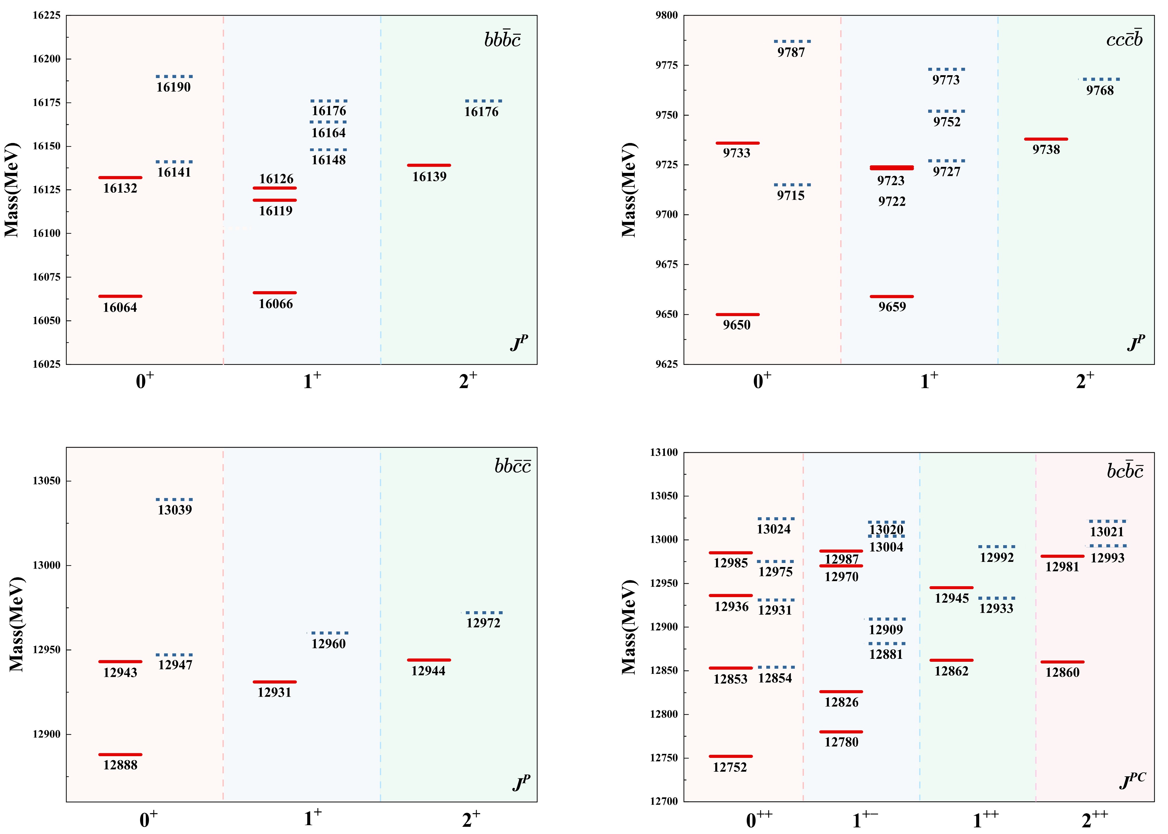
Figure 1. (color online) Mass spectrum of all-heavy tetraquarks with different flavors. The red solid lines and blue dashed lines represent the results obtained in this work and in our previous work [9], respectively. Masses are given in MeV.
The fall-apart decay properties of the
$ 1S $ -wave states of the tetraquarks$ bb\bar{b}\bar{c} $ ,$ cc\bar{c}\bar{b} $ ,$ bb\bar{c}\bar{c} $ , and$ bc\bar{b}\bar{c} $ are given in Table 6. It is found that the$ 1S $ -wave tetraquarks are likely to be narrow states, with fall-apart widths predicted to range from a few tenths of an MeV to several MeV. The main reason for the small fall-apart widths obtained in the present work is that the fall-apart decays are mainly driven by the chromo-magnetic (spin-spin) interaction$ V^{\mathrm{SS}} $ [71, 75], which is strongly suppressed by the heavy quark masses. Our predictions of narrow widths for the all-heavy tetraquark states are consistent with the expectations of the real and complex scaling methods [24, 25]. However, the coupled-channel calculation of Ref. [26] gives broad widths because the tetraquark states are treated there as meson-meson molecular states, leading to strong overlap with the continuum.$ J^P $ Mass $ \Gamma[\eta_b B_c^-] $ $ \Gamma[\eta_b B_c^{*-}] $ $ \Gamma[\Upsilon B_c^-] $ $ \Gamma[\Upsilon B_c^{*-}] $ $ \Gamma[\text{Sum}] $ $ bb\bar{b}\bar{c} $ $ 0^+ $ 16064 0.12 $ \cdots $ $ \cdots $ 1.13 1.25 16132 $<0.01 $ $ \cdots $ $ \cdots $ 0.44 0.44 $ 1^+ $ 16066 $ \cdots $ 0.70 0.37 0.78 1.85 16119 $ \cdots $ 0.96 0.66 1.34 2.96 16126 $ \cdots $ 0.01 0.03 0.10 0.14 $ 2^+ $ 16139 $ \cdots $ $ \cdots $ $ \cdots $ 0.86 0.86 $ J^P $ Mass $ \Gamma[\eta_c B_c^+] $ $ \Gamma[\eta_c B_c^{*+}] $ $ \Gamma[J/\psi B_c^+] $ $ \Gamma[J/\psi B_c^{*+}] $ $ \Gamma[\text{Sum}] $ $ cc\bar{c}\bar{b} $ $ 0^+ $ 9650 1.50 $ \cdots $ $ \cdots $ 0.85 2.35 9733 0.03 $ \cdots $ $ \cdots $ 2.65 2.68 $ 1^+ $ 9659 $ \cdots $ 0.14 0.20 0.12 0.46 9722 $ \cdots $ 1.08 0.01 0.05 1.14 9723 $ \cdots $ $<0.01 $ 0.60 0.23 0.83 $ 2^+ $ 9738 $ \cdots $ $ \cdots $ $ \cdots $ 0.18 0.18 $ J^P $ Mass $ \Gamma[B_c^-B_c^-] $ $ \Gamma[B_c^-B_c^{*-}] $ $ \Gamma[B_c^{*-} B_c^{*-}] $ $ \Gamma[\text{Sum}] $ $ bb\bar{c}\bar{c} $ $ 0^+ $ 12888 0.37 $ \cdots $ 0.14 0.51 12942 1.12 $ \cdots $ 0.87 1.99 $ 1^+ $ 12931 $ \cdots $ 0.10 $ \cdots $ 0.10 $ 2^+ $ 12944 $ \cdots $ $ \cdots $ 1.52 1.52 $ J^{PC} $ Mass $ \Gamma[\eta_b\eta_c] $ $ \Gamma[\eta_b J/\psi] $ $ \Gamma[\Upsilon\eta_c] $ $ \Gamma[\Upsilon J/\psi] $ $ \Gamma[B_c^+ B_c^-] $ $ \Gamma[B_c^+ B_c^{*-}+B_c^-B_c^{*+}] $ $ \Gamma[B_c^{*+} B_c^{*-}] $ $ \Gamma[\text{Sum}] $ $ bc\bar{b}\bar{c} $ $ 0^{++} $ 12752 0.37 $ \cdots $ $ \cdots $ 0.06 0.51 $ \cdots $ 2.41 3.35 12853 0.10 $ \cdots $ $ \cdots $ 0.50 0.01 $ \cdots $ 0.39 1.00 12936 1.58 $ \cdots $ $ \cdots $ $<0.01 $ 0.06 $ \cdots $ 1.69 3.33 12985 0.02 $ \cdots $ $ \cdots $ 2.01 0.60 $ \cdots $ 0.07 2.70 $ 1^{+-} $ 12780 $ \cdots $ $<0.01 $ 0.03 $ \cdots $ $ \cdots $ 0.21 0.14 0.38 12826 $ \cdots $ 0.03 $<0.01 $ $ \cdots $ $ \cdots $ 0.04 $<0.01 $ 0.07 12970 $ \cdots $ 0.02 0.05 $ \cdots $ $ \cdots $ 0.01 0.03 0.11 12987 $ \cdots $ 0.06 0.03 $ \cdots $ $ \cdots $ 0.01 0.01 0.10 $ 1^{++} $ 12862 $ \cdots $ $ \cdots $ $ \cdots $ $<0.01 $ $ \cdots $ $<0.01 $ $ \cdots $ $<0.01 $ 12945 $ \cdots $ $ \cdots $ $ \cdots $ $<0.01 $ $ \cdots $ $<0.01 $ $ \cdots $ $<0.01 $ $ 2^{++} $ 12860 $ \cdots $ $ \cdots $ $ \cdots $ 0.16 $ \cdots $ $ \cdots $ 0.27 0.43 12981 $ \cdots $ $ \cdots $ $ \cdots $ $<0.01 $ $ \cdots $ $ \cdots $ 0.08 0.08 Table 6. The predicted partial decay widths for the fall-apart decay processes of the 1S states in the
$ bb\bar{b}\bar{c} $ ,$ cc\bar{c}\bar{b} $ ,$ bb\bar{c}\bar{c} $ , and$ bc\bar{b}\bar{c} $ systems are presented. Forbidden decay channels are denoted by "$ \cdots $ ". The unit is MeV. -
For the
$ bb\bar{b}\bar{c} $ system, according to our quark model predictions, there are two$ J^P=0^+ $ states$ T_{(bb\bar{b}\bar{c})0^+}(16132) $ and$ T_{(bb\bar{b}\bar{c})0^+}(16064) $ , three$ J^P=1^+ $ states$ T_{(bb\bar{b}\bar{c})1^+}(16126) $ ,$ T_{(bb\bar{b}\bar{c})1^+}(16119) $ , and$ T_{(bb\bar{b}\bar{c})1^+}(16066) $ , and one$ J^P=2^+ $ state$ T_{(bb\bar{b}\bar{c})2^+}(16139) $ . From Table 5, one finds that these predicted states should be compact, with root-mean-square distances between any two inner quarks in the range$ (0.27,0.40) $ fm. For comparison, our predicted masses of the lowest$ 1S $ -wave$ bb\bar{b}\bar{c} $ states, together with those from other theoretical predictions, are shown in Fig. 1. Our results are compatible with predictions from the nonrelativistic quark model based on dynamic calculations [21−24] and diffusion Monte Carlo calculations [20], from the diquark model [27, 30, 31], and from the CGAN framework [53]. It should be mentioned that the results obtained with the complex scaling method [25] are systematically$ \sim450 $ MeV larger than ours. Since this difference is typical of a radial excitation energy, it is natural to ask whether these resonance states obtained in [25] may be$ 2S $ -wave$ bb\bar{b}\bar{c} $ states, and whether a similar situation occurs in other systems. On the other hand, the color-magnetic model [49] gives lower masses because it neglects the quark confinement potentials. -
The two
$ 0^+ $ states$ T_{(bb\bar{b}\bar{c})0^+}(16132) $ and$ T_{(bb\bar{b}\bar{c})0^+}(16064) $ exhibit a significant mass splitting,$ \Delta M\simeq 70 $ MeV, which is mainly due to spin-spin interactions. They are mixed states of two different color configurations,$ 6\otimes\bar{6} $ and$ \bar{3}\otimes 3 $ . The high-mass state$ T_{(bb\bar{b}\bar{c})0^+}(16132) $ is dominated by the$ \bar{3}\otimes 3 $ configuration, while the low-mass state$ T_{(bb\bar{b}\bar{c})0^+}(16064) $ is dominated by the$ 6\otimes\bar{6} $ configuration. More details can be found in Table 5. It should be mentioned that, with a more reliable trial wave function, the dominant components of the color configurations for the low- and high-mass states obtained in the present work differ from those in our previous work [9], except for a notable overall mass shift.The
$ T_{(bb\bar{b}\bar{c})0^+}(16132) $ and$ T_{(bb\bar{b}\bar{c})0^+}(16064) $ states lie about 400 MeV above the$ \eta_b B_c^- $ mass threshold. Their allowed fall-apart decay channels are$ \eta_b B_c^- $ and$ \Upsilon B_c^{*-} $ . The fall-apart decay properties are given in Table 6. Both$ T_{(bb\bar{b}\bar{c})0^+}(16132) $ and$ T_{(bb\bar{b}\bar{c})0^+}(16064) $ are predicted to be very narrow states with comparable fall-apart widths of$ \sim 1 $ MeV. They may have large decay rates into the$ \Upsilon B_c^* $ channel through fall-apart decays. The partial widths are predicted to be$ \begin{array}{l} \Gamma [T_{(bb\bar{b}\bar{c})0^+}(16064)\to\Upsilon B_c^*]\simeq 1.1\; \mathrm{MeV}, \end{array} $
(21) $ \begin{array}{l} \Gamma [T_{(bb\bar{b}\bar{c})0^+}(16132)\to\Upsilon B_c^*]\simeq 0.44\; \mathrm{MeV}. \end{array} $
(22) For
$ T_{(bb\bar{b}\bar{c})0^+}(16064) $ , the decay rate into the$ \eta_bB_c $ channel is also substantial, and the partial-width ratio between$ \Upsilon B_c^* $ and$ \eta_bB_c $ is predicted to be$ \mathcal{R}=\frac{\Gamma[T_{(bb\bar{b}\bar{c})0^+}(16064)\to\Upsilon B_c^*]}{\Gamma[T_{(bb\bar{b}\bar{c})0^+}(16064)\to\eta_bB_c]}\simeq 9.4. $
(23) -
Among the three
$ 1^+ $ states, the two high-lying states$ T_{(bb\bar{b}\bar{c})1^+}(16126) $ and$ T_{(bb\bar{b}\bar{c})1^+}(16119) $ are nearly degenerate. A significant mass gap,$ \Delta M\simeq 50 $ MeV, separates them from the low-lying state$ T_{(bb\bar{b}\bar{c})1^+}(16066) $ . The configuration mixing in these states is small. As shown in Table 5, the low-lying state$ T_{(bb\bar{b}\bar{c})1^+}(16066) $ is dominated by the$ 6\otimes\bar{6} $ configuration, whereas the two high-lying states$ T_{(bb\bar{b}\bar{c})1^+}(16126) $ and$ T_{(bb\bar{b}\bar{c})1^+}(16119) $ are dominated by the$ \bar{3}\otimes 3 $ configurations$ |{bb}_1^{\bar{3}}(\bar{b}\bar{c})_1^3\rangle_1^0 $ and$ |{bb}_1^{\bar{3}}(\bar{b}\bar{c})_0^3\rangle_1^0 $ , respectively.The decay properties are listed in Table 6. Both the
$ T_{(bb\bar{b}\bar{c})1^+}(16066) $ and$ T_{(bb\bar{b}\bar{c})1^+}(16119) $ states are narrow, with comparable widths of a few MeV. They have significant decay rates into the$ \Upsilon B_c^{-} $ ,$ \Upsilon B_c^{*-} $ , and$ \eta_b B_c^{*-} $ channels. The partial widths are predicted to be$ \begin{aligned}[b] \Gamma [T_{(bb\bar{b}\bar{c})1^+}(16066)\to &\Upsilon B_c/\Upsilon B_c^*/\eta_b B_c^{*}]\\ &\simeq 0.37/0.78/0.70\; \mathrm{MeV}, \end{aligned} $
(24) $ \begin{aligned}[b] \Gamma [T_{(bb\bar{b}\bar{c})1^+}(16119)\to &\Upsilon B_c/\Upsilon B_c^*/\eta_b B_c^{*}]\\ &\simeq 0.66/1.34/0.96\; \mathrm{MeV}. \end{aligned} $
(25) The
$ \Upsilon B_c $ channel could be promising for searching for these two$ 1^+ $ $ bb\bar{b}\bar{c} $ states. For the other high-lying state$ T_{(bb\bar{b}\bar{c})1^+}(16126) $ , however, the partial widths of the$ \Upsilon B_c^{-} $ ,$ \Upsilon B_c^{*-} $ , and$ \eta_b B_c^{*-} $ channels are two orders of magnitude smaller than those of the$ T_{(bb\bar{b}\bar{c})1^+}(16066) $ and$ T_{(bb\bar{b}\bar{c})1^+}(16119) $ states. This indicates that experimental observation of the$ T_{(bb\bar{b}\bar{c})1^+}(16126) $ state via the fall-apart decays may be challenging. -
The
$ 2^+ $ state$ T_{(bb\bar{b}\bar{c})2^+}(16139) $ , as a pure$ |{bb}_1^{\bar{3}}(\bar{b}\bar{c})_1^3\rangle_2^0 $ state, has a mass very close to those of the high-lying$ 0^+ $ and$ 1^+ $ states,$ T_{(bb\bar{b}\bar{c})0^+}(16132) $ and$ T_{(bb\bar{b}\bar{c})1^+}(16126) $ .The
$ \Upsilon B_c^* $ channel is the only allowed fall-apart decay channel of$ T_{(bb\bar{b}\bar{c})2^+}(16139) $ . The partial width is predicted to be$ \begin{array}{l} \Gamma [T_{(bb\bar{b}\bar{c})2^+}(16139)\to \Upsilon B_c^*]\simeq 0.86\; \mathrm{MeV}. \end{array} $
(26) -
The
$ cc\bar{c}\bar{b} $ system is analogous to the$ bb\bar{b}\bar{c} $ system owing to the same symmetry. There are two$ J^P=0^+ $ states,$ T_{(cc\bar{c}\bar{b})0^+}(9733) $ and$ T_{(cc\bar{c}\bar{b})0^+}(9650) $ ; three$ J^P=1^+ $ states,$ T_{(cc\bar{c}\bar{b})1^+}(9723) $ ,$ T_{(cc\bar{c}\bar{b})1^+}(9722) $ , and$ T_{(cc\bar{c}\bar{b})1^+}(9659) $ ; and one$ J^P=2^+ $ state,$ T_{(cc\bar{c}\bar{b})2^+}(9738) $ . From Table 5, one can see that these states are compact, with root-mean-square distances between any two inner quarks in the range$ (0.41, 0.51) $ fm. For comparison, Fig. 2 shows our predicted masses of the lowest$ 1S $ -wave$ cc\bar{c}\bar{b} $ states together with those from other theoretical predictions. As in the$ bb\bar{b}\bar{c} $ system, our results for the$ cc\bar{c}\bar{b} $ system are generally compatible with the nonrelativistic quark model predictions based on dynamic calculations [21−24] and diffusion Monte Carlo calculations [20], with the diquark model predictions [27, 30, 31], and with the results predicted by the CGAN framework [53]. It should be noted that the complex scaling method [25] again yields higher masses for the same reason discussed previously, whereas the color-magnetic model [49] shows the same deviation toward lower masses as in the$ bb\bar{b}\bar{c} $ system.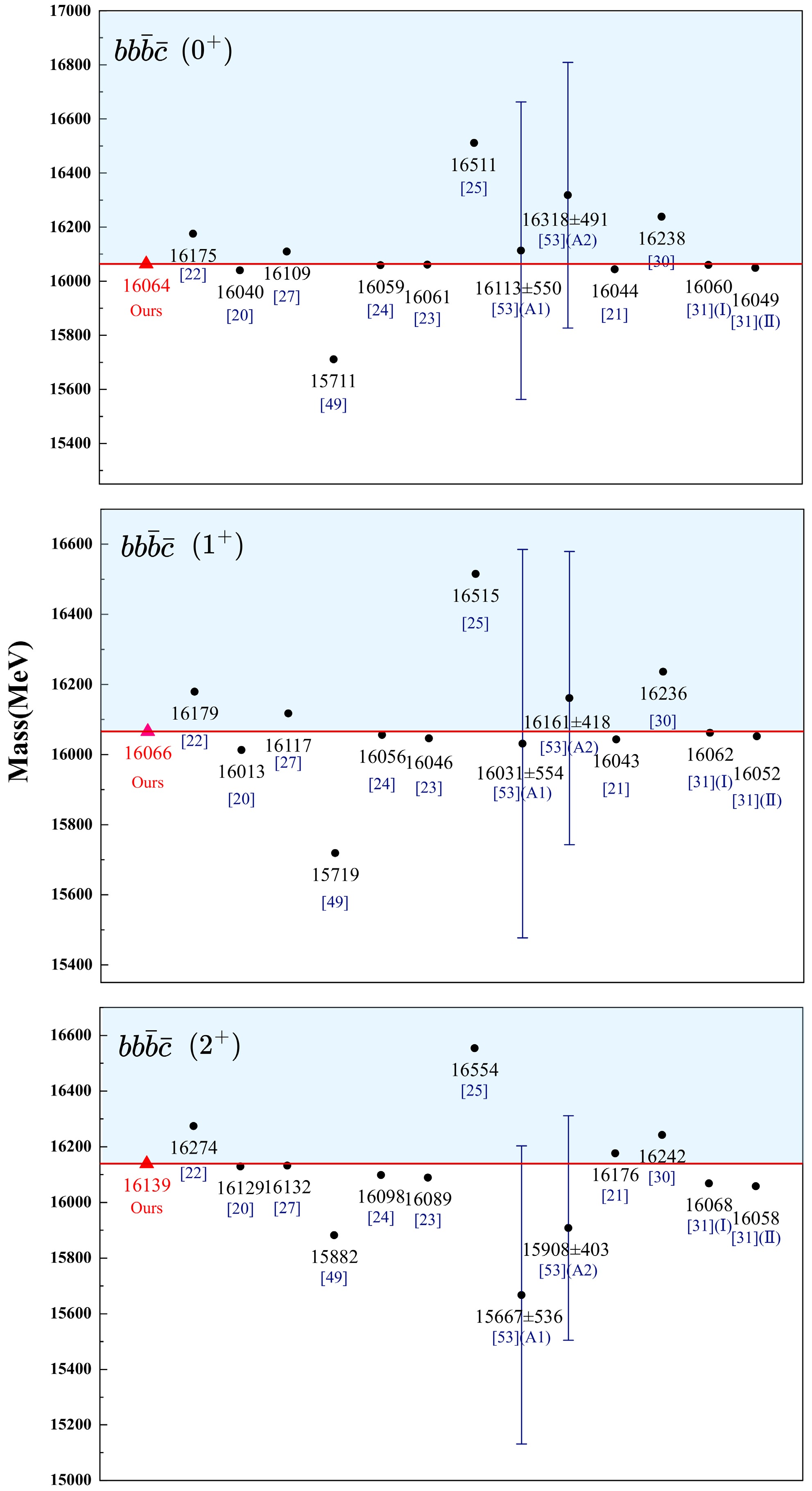
Figure 2. (color online) A comparison of the masses of the lowest
$ 1S $ -wave$ bb\bar{b}\bar{c} $ states across various model predictions. -
For the two states
$ T_{(cc\bar{c}\bar{b})0^+}(9733) $ and$ T_{(cc\bar{c}\bar{b})0^+}(9650) $ , the mass splitting is predicted to be$ \Delta M\simeq 90 $ MeV. The mass splitting between$ T_{(bb\bar{b}\bar{c})0^+}(16132) $ and$ T_{(bb\bar{b}\bar{c})0^+}(16064) $ ,$ \Delta M\simeq 70 $ MeV, is slightly smaller than that of the$ cc\bar{c}\bar{b} $ system, owing to the suppression of the heavy bottom quark. As shown in Table 5, the mixed states$ T_{(cc\bar{c}\bar{b})0^+}(9733) $ and$ T_{(cc\bar{c}\bar{b})0^+}(9650) $ are dominated by the$ \bar{3}\otimes 3 $ and$ 6\otimes\bar{6} $ components, respectively. The configuration mixing for the$ cc\bar{c}\bar{b} $ system is slightly stronger than that of the$ bb\bar{b}\bar{c} $ system, owing to a stronger spin-spin interaction.The decay properties are given in Table 6. It can be seen that both
$ 0^+ $ states have narrow fall-apart decay widths of about$ 3 $ MeV. The low-lying state$ T_{(cc\bar{c}\bar{b})0^+}(9650) $ predominantly decays into the$ \eta_c B_c $ and$ J/\psi B_c^* $ channels with partial decay widths of$ \begin{array}{l} \Gamma [T_{(cc\bar{c}\bar{b})0^+}(9650)\to J/\psi B_c^*/\eta_c B_c]\simeq 0.85/1.5\; \mathrm{MeV}. \end{array} $
(27) While the high-lying
$ 0^+ $ state$ T_{(cc\bar{c}\bar{b})0^+}(9733) $ exhibits a significant decay rate into the$ J/\psi B_c^* $ channel, with a partial decay width of$ \begin{array}{l} \Gamma [T_{(cc\bar{c}\bar{b})0^+}(9733)\to J/\psi B_c^*]\simeq 2.65\; \mathrm{MeV}, \end{array} $
(28) which is about a factor of 3 larger than that for
$ T_{(cc\bar{c}\bar{b})0^+}(9650)\to J/\psi B_c^* $ . The$ \eta_c B_c $ and$ J/\psi B_c^* $ could be promising channels in searches for the$ 0^+ $ $ cc\bar{c}\bar{b} $ states. -
The two high-lying
$ 1^+ $ states$ T_{(cc\bar{c}\bar{b})1^+}(9722) $ and$ T_{(cc\bar{c}\bar{b})1^+}(9723) $ are nearly degenerate. A significant mass gap$ \Delta M\simeq 40 $ MeV, originating from the difference in color structure, separates them from the low-lying state$ T_{(cc\bar{c}\bar{b})1^+}(9659) $ . Substantial configuration mixing exists among these$ 1^+ $ states. As shown in Table 5, the low-lying state$ T_{(cc\bar{c}\bar{b})1^+}(9659) $ , although a$ 6\otimes\bar{6} $ -dominant state, also contains a sizeable$ \bar{3}\otimes 3 $ component. In contrast, the two high-lying states$ T_{(cc\bar{c}\bar{b})1^+}(9722) $ and$ T_{(cc\bar{c}\bar{b})1^+}(9723) $ , in addition to their dominant$ \bar{3}\otimes 3 $ components$ |{cc}_1^{\bar{3}}(\bar{c}\bar{b})_1^3\rangle_1^0 $ and$ |{cc}_1^{\bar{3}}(\bar{c}\bar{b})_0^3\rangle_1^0 $ , contain a sizeable$ 6\otimes\bar{6} $ component.As shown in Table 6, the two high-lying states
$ T_{(cc\bar{c}\bar{b})1^+}(9722) $ and$ T_{(cc\bar{c}\bar{b})1^+}(9723) $ have comparable fall-apart decay widths of$ \sim1 $ MeV and predominantly decay into the$ \eta_c B_c^* $ and$ J/\psi B_c $ channels, respectively. The partial decay widths are predicted to be$ \begin{array}{l} \Gamma [T_{(cc\bar{c}\bar{b})1^+}(9722)\to \eta_c B_c^*]\simeq 1.08\; \mathrm{MeV}, \end{array} $
(29) $ \begin{array}{l} \Gamma [T_{(cc\bar{c}\bar{b})1^+}(9723)\to J/\psi B_c]\simeq 0.60\; \mathrm{MeV}. \end{array} $
(30) While the low-lying state
$ T_{(cc\bar{c}\bar{b})1^+}(9659) $ may have sizable decay rates into the$ \eta_c B_c^* $ ,$ J/\psi B_c $ , and$ J/\psi B_c^* $ channels, with comparable partial widths of$ \sim 0.1 $ –$ 0.2 $ MeV, the$ J/\psi B_c $ channel could be promising for searches for the$ 1^+ $ states$ T_{(cc\bar{c}\bar{b})1^+}(9723) $ and$ T_{(cc\bar{c}\bar{b})1^+}(9659) $ . -
The mass of the
$ 2^+ $ state$ T_{(cc\bar{c}\bar{b})2^+}(9738) $ , as a pure$ |{cc}_1^{\bar{3}}(\bar{c}\bar{b})_1^3\rangle_2^0 $ state, is very close to those of the high-lying$ 0^+ $ and$ 1^+ $ states,$ T_{(cc\bar{c}\bar{b})0^+}(9733) $ and$ T_{(cc\bar{c}\bar{b})1^+}(9723) $ .For
$ T_{(cc\bar{c}\bar{b})2^+}(9738) $ , the$ J/\psi B_c^* $ channel is the only allowed fall-apart decay mode. The partial width of this decay is predicted to be$ \begin{array}{l} \Gamma [T_{(cc\bar{c}\bar{b})2^+}(9738)\to J/\psi B_c^*]\simeq 0.18\; \mathrm{MeV}, \end{array} $
(31) which is comparable to that of
$ T_{(cc\bar{c}\bar{b})1^+}(9659,9723)\to J/\psi B_c^* $ , is, however, about an order of magnitude smaller than that of$ T_{(cc\bar{c}\bar{b})0^+}(9650,9733)\to J/\psi B_c^* $ . Thus, compared with these$ 0^+ $ states, the$ 2^+ $ state$ T_{(cc\bar{c}\bar{b})2^+}(9738) $ may be more difficult to discover in the$ J/\psi B_c^* $ channel. -
For the
$ bb\bar{c}\bar{c} $ system, our quark model predicts two$ J^P=0^+ $ states,$ T_{(bb\bar{c}\bar{c})0^+}(12942) $ and$ T_{(bb\bar{c}\bar{c})0^+}(12888) $ ; one$ J^P=1^+ $ state,$ T_{(bb\bar{c}\bar{c})1^+}(12931) $ ; and one$ J^P=2^+ $ state,$ T_{(bb\bar{c}\bar{c})2^+}(12944) $ . Table 5 shows that these four states are clustered within a very narrow mass region$ (12.88,12.95) $ GeV. They should be compact states, with root-mean-square distances between any two inner quarks in the range of$ (0.28,0.48) $ fm.For comparison, our predicted masses of the lowest
$ 1S $ -wave$ bb\bar{c}\bar{c} $ states are shown in Fig. 3, together with those from other theoretical predictions. Our results are generally compatible with the nonrelativistic quark model predictions based on dynamical calculations [10, 21−23] and diffusion Monte Carlo calculations [20], with the diquark model predictions [27, 30], and with the results predicted by the CGAN framework [53].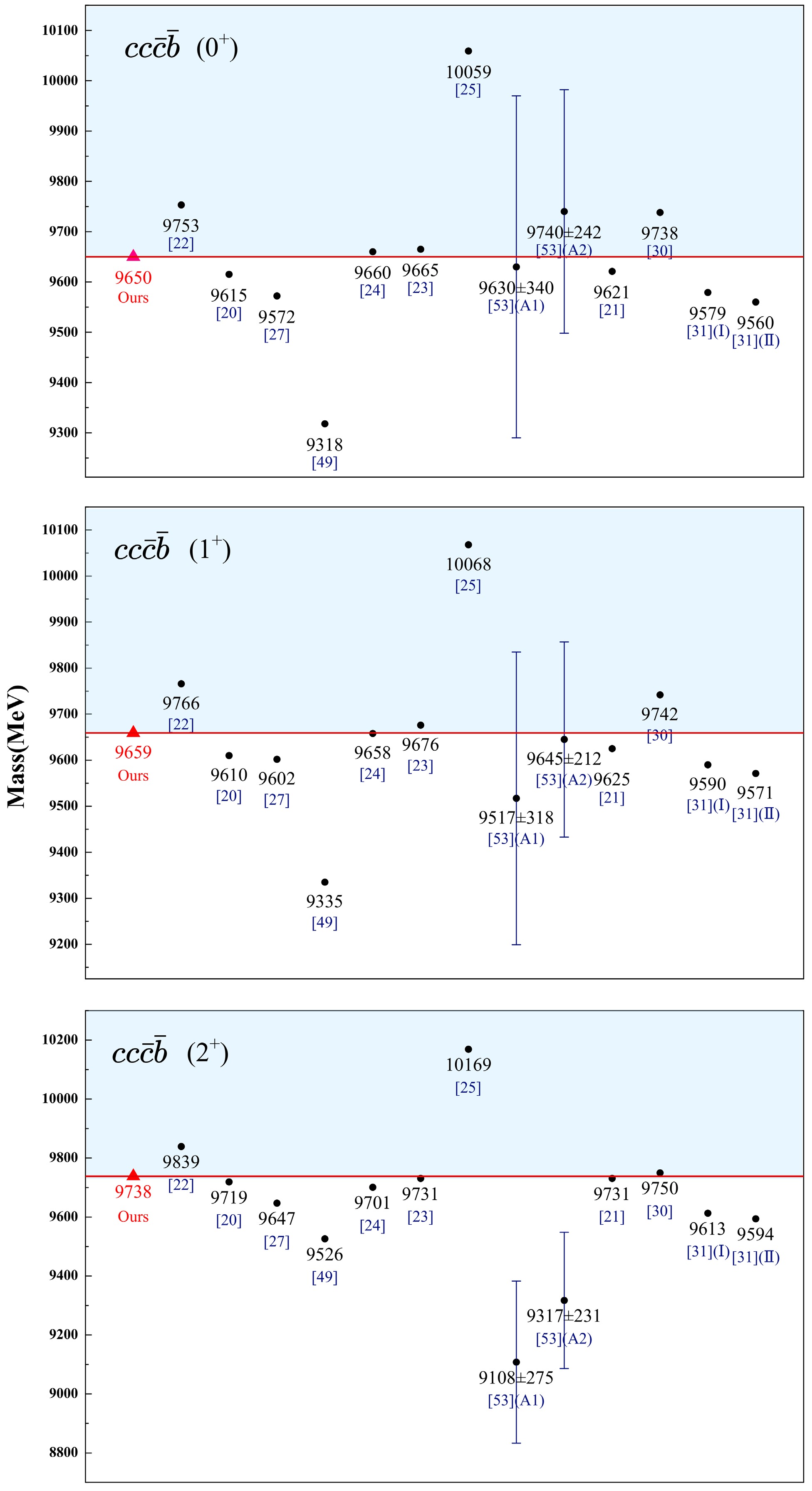
Figure 3. (color online) A comparison of the masses of the lowest
$ 1S $ -wave$ cc\bar{c}\bar{b} $ states predicted by various models.It should be noted that the complex scaling method [25] again gives higher masses for the same reason as discussed above. Several approaches give lower masses: the diquark models [11, 31], which assume a strong diquark correlation; the QCD sum rule calculation [33], which employs diquark-type interpolating currents; and the color-magnetic model [49], which neglects dynamical confinement.
-
The two
$ 0^+ $ states,$ T_{(bb\bar{c}\bar{c})0^+}(12942) $ and$ T_{(bb\bar{c}\bar{c})0^+}(12888) $ , exhibit a significant mass splitting of$ \Delta M\sim50 $ MeV. As shown in Table 5, they are mixed states of two different color configurations. The higher- and lower-mass states are dominated by the$ |\{bb\}_1^{\bar{3}}(\bar{c}\bar{c})_1^3\rangle_0^0 $ and$ |\{bb\}_0^6(\bar{c}\bar{c})_0^{\bar{6}}\rangle_0^0 $ components, respectively. The mass of$ |\{bb\}_0^6(\bar{c}\bar{c})_0^{\bar{6}}\rangle_0^0 $ is smaller than that of$ |\{bb\}_1^{\bar{3}}(\bar{c}\bar{c})_1^3\rangle_0^0 $ , consistent with the prediction of model I in Ref. [10].The
$ T_{(bb\bar{c}\bar{c})0^+}(12942) $ and$ T_{(bb\bar{c}\bar{c})0^+}(12888) $ lie about$ 300 $ MeV above the$ B_c^{*-}B_c^{*-} $ mass threshold. Their allowed fall-apart decay channels are$ B_c^-B_c^- $ and$ B_c^{*-}B_c^{*-} $ . As shown in Table 6, the$ T_{(bb\bar{c}\bar{c})0^+}(12942) $ and$ T_{(bb\bar{c}\bar{c})0^+}(12888) $ may be narrow states with widths of$ \sim2.0 $ MeV and$ \sim0.5 $ MeV, respectively. The$ T_{(bb\bar{c}\bar{c})0^+}(12942) $ has comparable decay rates into both the$ B_c^*B_c^* $ and$ B_cB_c $ channels. The partial widths are predicted to be$ \begin{array}{l} \Gamma [T_{(bb\bar{c}\bar{c})0^+}(12942)\to B_cB_c/B_c^*B_c^*]\simeq 1.12/0.87\; \mathrm{MeV}, \end{array} $
(32) The low-mass
$ 0^+ $ state$ T_{(bb\bar{c}\bar{c})0^+}(12888) $ predominantly decays into the$ B_cB_c $ channel with a partial width of$ \begin{array}{l} \Gamma [T_{(bb\bar{c}\bar{c})0^+}(12888)\to B_cB_c]\simeq 0.37\; \mathrm{MeV}, \end{array} $
(33) whereas the decay rate into the
$ B_c^*B_c^* $ channel is sizable. The ratio of the partial widths for these two channels is predicted to be$ \mathcal{R}=\frac{\Gamma[T_{(bb\bar{c}\bar{c})0^+}(12888)\to B_c^*B_c^*]} {\Gamma[T_{(bb\bar{c}\bar{c})0^+}(12888)\to B_cB_c]}\simeq 0.4. $
(34) $ B_cB_c $ could be a promising channel for experimental searches for the$ 0^+ $ $ bb\bar{c}\bar{c} $ states. -
As the highest-mass state in the
$ bb\bar{c}\bar{c} $ system, the$ T_{(bb\bar{c}\bar{c})2^+}(12944) $ lies only about$ 13 $ MeV above the$ 1^+ $ state$ T_{(bb\bar{c}\bar{c})1^+}(12931) $ and is also nearly degenerate with the high-lying$ 0^+ $ state$ T_{(bb\bar{c}\bar{c})0^+}(12942) $ , owing to their similar color-spin structures.For the
$ T_{(bb\bar{c}\bar{c})1^+}(12931) $ and$ T_{(bb\bar{c}\bar{c})2^+}(12944) $ , the allowed fall-apart decay channels are$ B_cB_c^* $ and$ B_c^*B_c^* $ , respectively. The partial widths are predicted to be$ \begin{array}{l} \Gamma [T_{(bb\bar{c}\bar{c})1^+}(12931)\to B_cB_c^*]\simeq 0.10\; \mathrm{MeV}, \end{array} $
(35) $ \begin{array}{l} \Gamma [T_{(bb\bar{c}\bar{c})2^+}(12944)\to B_c^*B_c^*]\simeq 1.52\; \mathrm{MeV}. \end{array} $
(36) -
For the
$ bc\bar{b}\bar{c} $ system, because the Pauli principle imposes no constraints, there are more states than in the other systems. Our quark model calculations yield four$ J^P=0^{++} $ states$ T_{(bc\bar{b}\bar{c})0^{++}}(12985/12936/12853/12752) $ , four$ J^P=1^{+-} $ states$ T_{(bc\bar{b}\bar{c})1^{+-}}(12987/12970/12826/12780) $ , two$ J^P=1^{++} $ states$ T_{(bc\bar{b}\bar{c})1^{++}}(12945/12862) $ , and two$ J^P=2^{++} $ states$ T_{(bc\bar{b}\bar{c})2^{++}}(12981/12860) $ . These twelve states are distributed over a relatively broad mass range,$ (12.75,12.99) $ GeV. As shown in Table 5, these states should be compact, with root-mean-square distances between any two constituent quarks in the range$ (0.29, 0.47) $ fm. For comparison, our predicted masses for the lowest$ 1S $ -wave$ bc\bar{b}\bar{c} $ states, together with those from other theoretical predictions, are shown in Fig. 4. Our results are generally compatible with the nonrelativistic quark model predictions based on dynamical calculations [21−23], the diquark model predictions [27, 28], and those from the CGAN framework [53]. It should be noted that the complex scaling method [25] again yields higher masses for the same reason discussed previously, whereas the Bethe-Salpeter equation approach [51] yields higher masses because it introduces a different interaction kernel. Several approaches yield lower masses: the diquark model [11], which assumes a strong diquark correlation; the QCD sum rule calculation [32], which employs diquark-type interpolating currents; the color-magnetic models [49, 50], which neglect dynamical confinement; and the bosonic algebraic approach [52], which adopts a different parametrization of the dynamics.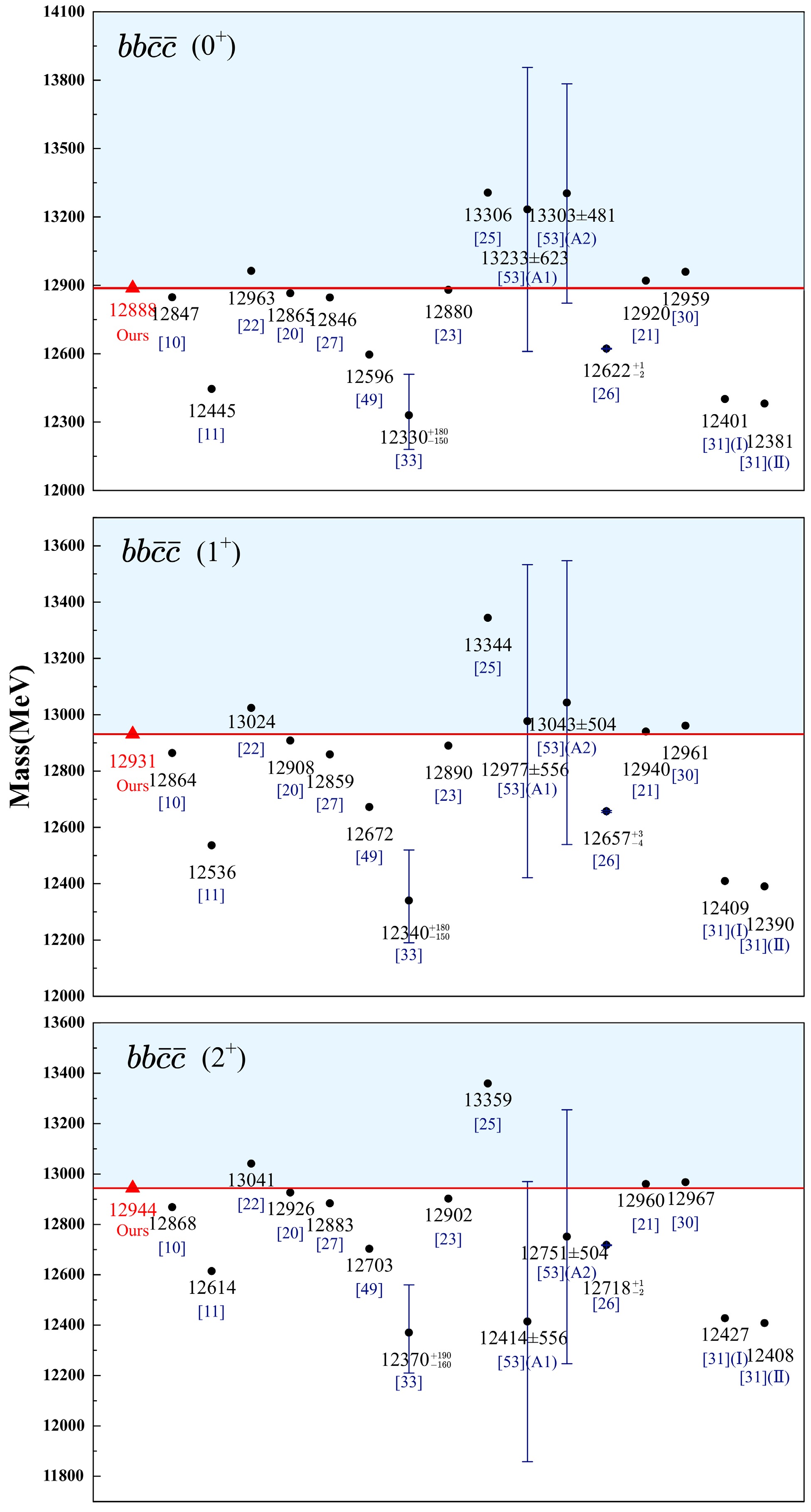
Figure 4. (color online) A comparison of the masses of the lowest
$ 1S $ -wave$ bb\bar{c}\bar{c} $ states predicted by various models.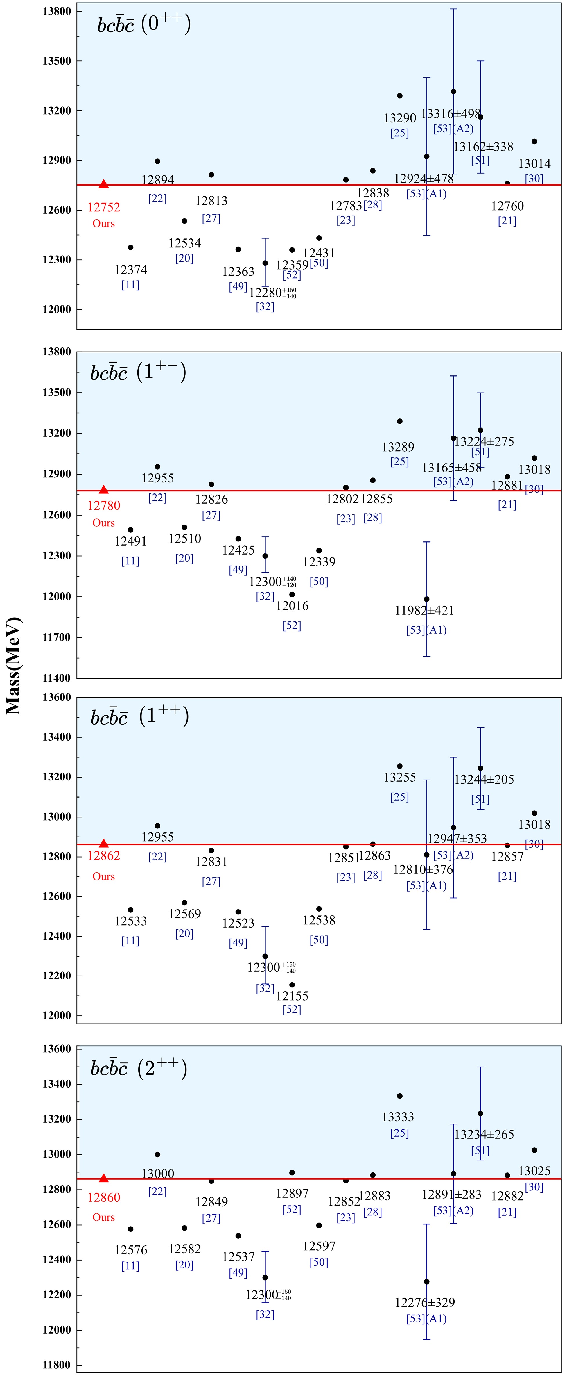
Figure 5. (color online) A comparison of the masses of the lowest
$ 1S $ -wave$ bc\bar{b}\bar{c} $ states across various model predictions. -
For the four
$ J^P=0^{++} $ states, there is strong configuration mixing between the$ 6\otimes\bar{6} $ and$ \bar{3}\otimes 3 $ configurations. Table 5 shows that the dominant color component of the two high-lying states$ T_{(bc\bar{b}\bar{c})0^{++}}(12985) $ and$ T_{(bc\bar{b}\bar{c})0^{++}}(12936) $ is$ \bar{3}\otimes 3 $ , whereas for the two low-lying states$ T_{(bc\bar{b}\bar{c})0^{++}}(12853) $ and$ T_{(bc\bar{b}\bar{c})0^{++}}(12752) $ , the dominant color component is$ 6\otimes\bar{6} $ . There is a significant mass interval,$ \Delta M\sim 50-100 $ MeV, between any two adjacent states.As shown in Table 6, the two low-lying
$ 0^{++} $ states$ T_{(bc\bar{b}\bar{c})0^{++}}(12752) $ and$ T_{(bc\bar{b}\bar{c})0^{++}}(12853) $ have narrow fall-apart widths of$ \sim 3 $ and$ \sim 1 $ MeV, respectively. The partial widths of their main decay channels are predicted to be$ \begin{aligned}[b] \Gamma [T_{(bc\bar{b}\bar{c})0^{++}}(12752)\to& \eta_b\eta_c/B_c^+B_c^-/B_c^{*+}B_c^{*-}]\\ & \simeq 0.37/0.51/2.4\; \mathrm{MeV}. \end{aligned} $
(37) $ \begin{aligned}[b] \Gamma [T_{(bc\bar{b}\bar{c})0^{++}}(12853)\to& \eta_b\eta_c/\Upsilon J/\psi/B_c^{*+}B_c^{*-}]\\ & \simeq 0.10/0.50/0.39\; \mathrm{MeV}. \end{aligned} $
(38) The two high-lying
$ 0^{++} $ states$ T_{(bc\bar{b}\bar{c})0^{++}}(12985) $ and$ T_{(bc\bar{b}\bar{c})0^{++}}(12936) $ have comparable fall-apart widths of$ \sim 3 $ MeV. The$ T_{(bc\bar{b}\bar{c})0^{++}}(12985) $ predominantly decays into the$ \Upsilon J/\psi $ and$ B_c^+B_c^- $ channels, with partial widths of$ \begin{array}{l} \Gamma [T_{(bc\bar{b}\bar{c})0^{++}}(12985)\to \Upsilon J/\psi/B_c^+B_c^-]\simeq 2.0/0.60\; \mathrm{MeV}. \end{array} $
(39) While the highest-lying state
$ T_{(bc\bar{b}\bar{c})0^{++}}(12936) $ predominantly decays into the$ \eta_b\eta_c $ and$ B_c^{*+}B_c^{*-} $ channels, with partial widths of$ \begin{array}{l} \Gamma [T_{(bc\bar{b}\bar{c})0^{++}}(12936)\to \eta_b\eta_c/B_c^{*+}B_c^{*-}]\simeq 1.6/1.7\; \mathrm{MeV}. \end{array} $
(40) The
$ \eta_b\eta_c $ ,$ \Upsilon J/\psi $ , and$ B_c^+B_c^- $ channels could be promising for experimental searches for these$ 0^{++} $ $ bc\bar{b}\bar{c} $ states. -
For the four
$ J^P=1^{+-} $ states, there is also strong configuration mixing between the$ 6\otimes\bar{6} $ and$ \bar{3}\otimes 3 $ configurations. For the two high-lying states$ T_{(bc\bar{b}\bar{c})1^{+-}}(12987) $ and$ T_{(bc\bar{b}\bar{c})1^{+-}}(12970) $ , the dominant color component is$ \bar{3}\otimes 3 $ . For the two low-lying states$ T_{(bc\bar{b}\bar{c})1^{+-}}(12826) $ and$ T_{(bc\bar{b}\bar{c})1^{+-}}(12780) $ , by contrast, the dominant color component is$ 6\otimes\bar{6} $ . Further details can be found in Table 5.Among these
$ 1^{+-} $ states, as shown in Table 6, the lowest state$ T_{(bc\bar{b}\bar{c})1^{+-}}(12780) $ has a relatively broad fall-apart width of$ \sim 0.4 $ MeV. It may have sizable decay rates into the$ B_cB_c^*=B_c^+B_c^{*-}+B_c^{*+}B_c^{-} $ and$ B_c^{*+}B_c^{*-} $ channels, with comparable partial widths.$ \begin{array}{l} \Gamma [T_{(bc\bar{b}\bar{c})1^{+-}}(12780)\to B_cB_c^*/B_c^{*+}B_c^{*-}]\simeq 0.21/0.14\; \mathrm{MeV}. \end{array} $
(41) For the other
$ 1^{+-} $ states, the fall-apart decay widths are predicted to be$ \sim100 $ keV. These states may therefore be difficult to observe through their fall-apart decay channels. -
From Table 5, one can see that there is slight mixing between the
$ 6\otimes\bar{6} $ and$ \bar{3}\otimes 3 $ configurations in the$ 1^{++} $ and$ 2^{++} $ states. The low-mass state$ T_{(bc\bar{b}\bar{c})1^{++}}(12862) $ and the high-mass state$ T_{(bc\bar{b}\bar{c})1^{++}}(12945) $ are governed by the$ 6\otimes\bar{6} $ and$ \bar{3}\otimes 3 $ components, respectively. However, in the$ 2^{++} $ sector, the situation is reversed: the low-mass state$ T_{(bc\bar{b}\bar{c})2^{++}}(12860) $ and the high-mass state$ T_{(bc\bar{b}\bar{c})2^{++}}(12981) $ are governed by the$ \bar{3}\otimes 3 $ and$ 6\otimes\bar{6} $ components, respectively. The mass splitting between the two states with the same spin-parity quantum numbers is significant, reaching up to$ \Delta M\sim 100 $ MeV. It should be mentioned that$ T_{(bc\bar{b}\bar{c})1^{++}}(12862) $ and$ T_{(bc\bar{b}\bar{c})2^{++}}(12860) $ are highly degenerate owing to their similar spin-color structures.As shown in Table 6, the low-mass
$ 2^{++} $ state$ T_{(bc\bar{b}\bar{c})2^{++}}(12860) $ has a narrow fall-apart width of$ \sim 0.4 $ MeV. It has significant decay rates into both the$ \Upsilon J/\psi $ and$ B_c^{*+}B_c^{*-} $ channels, with partial widths of$ \begin{array}{l} \Gamma [T_{(bc\bar{b}\bar{c})2^{++}}(12860)\to \Upsilon J/\psi/B_c^{*+}B_c^{*-}]\simeq 0.16/0.27\; \mathrm{MeV}. \end{array} $
(42) This state may have the potential to be observed in future experiments. For the two
$ 1^{++} $ states and the high-mass$ 2^{++} $ state, Table 6 shows that their fall-apart decay channels are nearly forbidden. Therefore, the possibility of establishing these states via fall-apart decay processes may be very small. -
In this work, we carry out a precise calculation of the mass spectrum of the tetraquarks
$ bb\bar{b}\bar{c} $ ,$ cc\bar{c}\bar{b} $ ,$ bb\bar{c}\bar{c} $ , and$ bc\bar{b}\bar{c} $ using a nonrelativistic potential model based on the reliable ECG numerical method. A complete mass spectrum of the$ 1S $ states is obtained. The masses of the$ 1S $ -wave states for the$ bb\bar{b}\bar{c} $ ,$ cc\bar{c}\bar{b} $ ,$ bb\bar{c}\bar{c} $ , and$ bc\bar{b}\bar{c} $ systems are predicted to lie in the ranges$ \sim(16.06,16.14) $ ,$ \sim(9.65,9.74) $ ,$ \sim(12.89,12.94) $ , and$ \sim(12.75,12.99) $ GeV, respectively. All states are compact structures and lie significantly above their dissociation thresholds into two ground-state mesons. Compared with our previous rough predictions, the masses of all states predicted with the reliable ECG method are found to be shifted downward by around$ 30-100 $ MeV, and the mass splittings are also notably modified.Moreover, using the obtained masses and wave functions of the
$ 1S $ -wave states for the$ bb\bar{b}\bar{c} $ ,$ cc\bar{c}\bar{b} $ ,$ bb\bar{c}\bar{c} $ , and$ bc\bar{b}\bar{c} $ systems, we further evaluate the fall-apart decay properties within a quark exchange model. The all-heavy tetraquarks are likely to be narrow states; their fall-apart widths are predicted to range from a few tenths to several MeV. The partial widths of the fall-apart decay channels for each$ 1S $ -wave state are presented. Some$ 1S $ states of the$ bb\bar{b}\bar{c} $ ,$ cc\bar{c}\bar{b} $ ,$ bb\bar{c}\bar{c} $ , and$ bc\bar{b}\bar{c} $ systems could be searched for via their optimal fall-apart decay channels. Based on the calculated decay widths and the feasibility of final-state reconstruction, we list the most promising states and their optimal channels in Table 7.System $ J^{P(C)} $ Mass (MeV) Optimal channel(s) Width (MeV) $ bb\bar{b}\bar{c} $ $ 0^+ $ 16064 $ \Upsilon B_c^* $ 1.13 $ 0^+ $ 16132 $ \Upsilon B_c^* $ 0.44 $ 1^+ $ 16066 $ \Upsilon B_c $ 0.37 $ 1^+ $ 16119 $ \Upsilon B_c $ 0.66 $ 2^+ $ 16139 $ \Upsilon B_c^* $ 0.86 $ cc\bar{c}\bar{b} $ $ 0^+ $ 9650 $ \eta_c B_c $ /$ J/\psi B_c^* $ 1.50 / 0.85 $ 0^+ $ 9733 $ J/\psi B_c^* $ 2.65 $ 1^+ $ 9659 $ J/\psi B_c $ 0.20 $ 1^+ $ 9723 $ J/\psi B_c $ 0.60 $ bb\bar{c}\bar{c} $ $ 0^+ $ 12888 $ B_c B_c $ 0.37 $ 0^+ $ 12942 $ B_c B_c $ 1.12 $ 2^+ $ 12944 $ B_c^* B_c^* $ 1.52 $ bc\bar{b}\bar{c} $ $ 0^{++} $ 12752 $ \eta_b\eta_c $ /$ B_c^+ B_c^- $ 0.37 / 0.51 $ 0^{++} $ 12853 $ \Upsilon J/\psi $ 0.50 $ 0^{++} $ 12936 $ \eta_b\eta_c $ 1.58 $ 0^{++} $ 12985 $ \Upsilon J/\psi $ /$ B_c^+ B_c^- $ 2.01 / 0.60 $ 1^{+-} $ 12780 $ B_c B_c^* $ /$ B_c^{*+} B_c^{*-} $ 0.21 / 0.14 $ 2^{++} $ 12860 $ \Upsilon J/\psi $ /$ B_c^{*+} B_c^{*-} $ 0.16 / 0.27 Table 7. A concise list of the most promising tetraquark states, including their quantum numbers, mass ranges, and optimal decay channels
Finally, it should be noted that the states obtained in the present quark model framework (often called bare states) are not strictly physical states, since the coupled-channel effects from the decay channels (the two-hadron continuum) are neglected in this approximation. Fortunately, the narrow fall-apart decay widths of the quark model states indicate that the mass-shift contributions from the continuum couplings should not be significant. On the other hand, mixing with the meson-meson states is also suppressed, since the obtained bare compact states lie far above the meson-meson thresholds. Thus, the predicted masses and widths for the bare compact states might be comparable to those of physical resonances if they are observed experimentally in the invariant mass spectra of final states.
All-heavy tetraquarks with different flavors
- Received Date: 2026-05-28
- Available Online: 2027-02-01
Abstract: Within the framework of a nonrelativistic potential quark model, we perform a precise calculation of the mass spectrum of the all-heavy tetraquarks with different flavors, $bb\bar{b}\bar{c}$, $cc\bar{c}\bar{b}$, $bb\bar{c}\bar{c}$, and $bc\bar{b}\bar{c}$, using the explicitly correlated Gaussian method. A complete mass spectrum for the $1S$ states is obtained. For the $bb\bar{b}\bar{c}$, $cc\bar{c}\bar{b}$, $bb\bar{c}\bar{c}$, and $bc\bar{b}\bar{c}$ systems, the $1S$ states are predicted to lie in the mass ranges of $\sim(16.06,16.14)$, $\sim(9.65,9.74)$, $\sim(12.89,12.94)$, and $\sim(12.75,12.99)$ GeV, respectively. Furthermore, using the obtained masses and wave functions, we evaluate the fall-apart decay properties within a quark-exchange model. The results show that the $1S$ states of the all-heavy tetraquarks with different flavors may have narrow fall-apart decay widths, ranging from a few tenths of an MeV to several MeV. Some all-heavy tetraquarks with different flavors could be searched for at the LHC through their optimal fall-apart decay channels, such as $\Upsilon J/\psi$, $\Upsilon B_c^-$, and $J/\psi B_c^+$.



 DownLoad: