


 Abstract
 HTML
 Reference
 Related
 PDF



-
β decay is one of the most fundamental decay modes of unstable nuclei and plays an important role in nuclear physics, particle physics, and nuclear astrophysics. Nuclear β-decay half-lives are sensitive to nuclear masses [1], shell gaps [2, 3], and deformation [4], thereby providing insight into nuclear structure and the effective nucleon-nucleon interaction. In nuclear astrophysics, β-decay half-lives are key inputs for rapid neutron capture process (r-process) nucleosynthesis [5], as they govern the timescale of matter flow toward heavier nuclei and influence the final abundance pattern [6]. r-process nucleosynthesis simulations involve thousands of neutron-rich nuclei [7], many of which are short-lived and experimentally inaccessible. According to the NUBASE2020 database, experimental β-decay half-lives are available for about 2400 ground-state nuclei [8]. Therefore, reliable theoretical predictions of β-decay half-lives are essential for providing the nuclear inputs required for nuclei beyond experimental reach.
Currently, microscopic theoretical studies of β-decay half-lives are mainly based on the shell model and the pnQRPA. The shell model provides a microscopic description of nuclear β decay, with many-particle–many-hole correlations incorporated into the nuclear wave functions through configuration mixing [9]. For example, systematic shell-model calculations have been performed for the β-decay half-lives and neutron emission probabilities of r-process waiting-point nuclei at the neutron magic numbers
$ N=50 $ , 82, and 126 [10]. However, the rapidly increasing dimension of the shell-model configuration space limits its applicability to global calculations across the nuclear chart.The QRPA provides a microscopic description of nuclear excitations while remaining computationally feasible for large-scale calculations, making it well suited for global studies of β decay. Early global calculations combined the finite-range droplet model (FRDM) with the QRPA to calculate β-decay half-lives within the Gamow-Teller (GT) approximation for 8979 nuclei, covering a broad region from 16O to 339136 [11]. The updated FRDM + QRPA calculations were extended to 9318 nuclei and incorporated both GT and first-forbidden (FF) contributions [12]. This approach is computationally efficient and incorporates nuclear deformation, but the ground state and QRPA excitations are described by different interactions and are therefore not fully self-consistent. A more self-consistent treatment can be achieved by combining the QRPA with density functional theory. In the non-relativistic framework, a global calculation of β-decay half-lives using spherical pnQRPA based on the Skyrme Hartree-Fock-Bogoliubov (SHFB) framework has been performed for 5581 nuclei with
$ Z=8 $ –110, where the isoscalar pairing strengths are determined by a Bayesian neural network trained on experimental data [13]. To account for deformation effects, the finite-amplitude method (FAM) has been employed to solve deformed QRPA equations on top of SHFB ground states [14], and its extension to odd-mass and odd-odd nuclei has led to systematic calculations for 3983 neutron-rich nuclei with$ 20\leq Z\leq 110 $ [15]. In these approaches, the nuclear ground state and QRPA response are treated consistently within the same functional SKO′, providing a more self-consistent description than the FRDM + QRPA approach.However, these calculations remain within a non-relativistic framework. Covariant density functional theory (CDFT) incorporates Lorentz invariance and naturally describes the spin-orbit interaction [16, 17]. In the relativistic framework, systematic calculations of β-decay half-lives have been performed within the spherical relativistic QRPA framework based on the relativistic Hartree-Bogoliubov (RHB) model [18]. These calculations include both GT and FF transitions and cover 5409 neutron-rich nuclei with
$ 8\leq Z \leq 110 $ . Recently, self-consistent relativistic QRPA calculations based on RHB ground states have been extended to axially deformed nuclei, using the DD-PC1 and DD-PCX functionals to calculate β-decay half-lives for about 4800 neutron-rich nuclei with$ Z=20 $ –110 [19].Despite the progress of relativistic QRPA approaches, exchange terms are neglected in conventional applications of CDFT, which limits the consistency between the nuclear ground state and the particle-hole residual interaction in QRPA. In the Hartree approximation, exchange terms are neglected, leaving the pion contribution to the charge-exchange residual interaction unconstrained by the ground state and requiring phenomenological adjustment from the GT response. Including the Fock terms restores the nonzero contribution of pion-meson exchange terms to ground-state properties, eliminating the need for free adjustment in the excited-state calculation [20]. Based on the RHFB framework with the PKO1 functional, systematic calculations of β-decay half-lives have been performed for even-even nuclei with
$ 20\leq Z\leq50 $ [21]. However, the explicit treatment of Fock terms substantially increases the computational cost, making such calculations difficult to extend to the entire nuclear chart. As a solution, in relativistic point-coupling models, exchange terms can be localized via the Fierz transformation without additional numerical complexity [22], an approach that has been incorporated into the PCF-PK1 functional [23].Apart from the treatment of the particle-hole residual interaction, the quality of β-decay half-life calculations is also closely related to the underlying single-particle structure of the nuclear ground state. In particular, the Landau effective mass
$ M_L^* $ plays an important role in determining the single-particle level density around the Fermi surface, which strongly affects the distribution of GT strength and half-lives. The D3C* functional used in Ref. [18] was developed from D3C by increasing the Landau effective mass from$ M_L^*=0.71M $ to$ 0.79M $ [24]. This larger Landau mass increases the transition energies, consequently reducing the calculated half-lives compared with experiment. In the PCF-PK1 functional, the Landau effective mass is also increased to$ M_L^*=0.85M $ through the inclusion of an isoscalar tensor coupling [23], which is expected to make it more suitable for describing β-decay half-lives than conventional relativistic density functionals.The PCF-PK1 functional incorporates localized Fock terms and the isoscalar tensor coupling, providing a fully self-consistent treatment of the nuclear ground state and excited states, as well as a relatively large Landau effective mass. The pnQRPA
1 based on localized RHFB with the PCF-PK1 interaction has been established, and it showed that the increased Landau mass helps produce shorter β-decay half-lives and hence closer agreement with experiment1 .Building on these advantages, in this work we perform systematic calculations of β-decay half-lives for even-even, odd-A, and odd-odd nuclei with
$ 8\leq Z \leq 120 $ based on the localized RHFB + pnQRPA theory. As a first step, we adopt the spherical approximation and include only allowed GT transitions. The pnQRPA theoretical framework with the PCF-PK1 functional and the numerical details are presented in Secs. 2 and 3. The predictive power of PCF-PK1 under the spherical approximation and comparisons among different calculations are presented in Sec. 4. The improvement of β-decay half-lives using a neural network is given in Sec. 5. Finally, we provide concluding remarks in Sec. 6. -
The nuclear ground state is described within the localized RHFB theory using the PCF-PK1 point-coupling density functional and a finite-range separable pairing force. The canonical basis obtained from the localized RHFB ground state is then used to construct the pnQRPA. The GT transition strengths and corresponding
$ \beta^- $ -decay half-lives are calculated within the pnQRPA framework. -
The effective Lagrangian density of the relativistic point-coupling model used in this work comprises free-nucleon, four-fermion, derivative, and electromagnetic terms [23],
$ \begin{aligned} \mathcal L={\cal{L}}_{{\rm{free}}}+{\cal{L}}_{{\rm{4f}}} + {\cal{L}}_{{\rm{der}}}+{\cal{L}}_{{\rm{em}}} \, , \end{aligned} $
(1) with
$ \begin{aligned} {\cal{L}}_{{\rm{free}}}=\bar\psi( \mathrm i\gamma_\mu\partial^\mu-M)\psi, \end{aligned} $
(2a) $ \begin{aligned} {\cal{L}}_{{\rm{4f}}}=-\frac12\sum_{i\in{\cal{C}}}\alpha_i (\bar\psi\Gamma_i\psi)(\bar\psi\Gamma^i\psi), \end{aligned} $
(2b) $ \begin{aligned} {\cal{L}}_{{\rm{der}}}=-\frac12\delta_S \partial_\mu(\bar\psi\psi)\partial^\mu(\bar\psi\psi), \end{aligned} $
(2c) $ \begin{aligned} {\cal{L}}_{{\rm{em}}}=-e\bar\psi\gamma_\mu\frac{1-\tau_3}{2}\psi A^\mu -\frac14F_{\mu\nu}F^{\mu\nu} \, . \end{aligned} $
(2d) Here, ψ and M denote the nucleon field and mass, respectively.
$ \alpha_i $ and$ \delta_S $ are coupling strengths.$ F_{\mu\nu}=\partial_\mu A_\nu-\partial_\nu A_\mu $ , where$ A^\mu $ is the electromagnetic four-potential. The vertices$ \Gamma_i $ are constructed by combining the isospin factors$ \{1,\boldsymbol\tau\} $ with the Dirac matrices$ \{1,\gamma_\mu,\sigma_{\mu\nu}, \gamma_5,\gamma_5\gamma_\mu\} $ , where$ \sigma_{\mu\nu}= \mathrm i[\gamma_\mu,\gamma_\nu]/2 $ . The five Dirac structures correspond to the scalar (S), vector (V), tensor (T), pseudoscalar ($ PS $ ), and pseudovector (PV) channels, respectively. Combining each of these structures with either the isoscalar or isovector isospin factor yields the ten channels.$ \begin{aligned} {\cal{C}}=\{ S,tS,V,tV,T,tT,PS,tPS,PV,tPV \} \, , \end{aligned} $
(3) where the prefix t denotes an isovector channel. The convention
$ \tau_3=+1 (-1) $ is adopted for neutrons (protons).A Legendre transformation of the Lagrangian in Eq.(1) yields the Hamiltonian, whose expectation value in the Hartree-Fock (HF) vacuum defines
$ E_{{\rm{CDF}}}[\rho] $ , where ρ denotes the density matrix. The four-fermion energy includes direct (Hartree) and exchange (Fock) contributions with coupling constants$ \alpha_j^{\rm{HF}} $ , whereas the derivative and electromagnetic terms are treated at the Hartree level. The Fierz transformation rewrites the four-fermion exchange contributions as local direct terms, thereby allowing the exchange contributions to be incorporated at the Hartree level [22, 23]. The coupling constants$ \alpha_i $ of these localized direct terms are related to the HF coupling constants by$ \begin{aligned} \alpha_i=\sum_j C_{ij} \alpha_j^{{\rm{HF}}} \, , \end{aligned} $
(4) where the matrix C is determined by the Fierz transformation [23]. In the PCF-PK1 density functional, the localized S, tS, V, tV, and T couplings are independent, whereas the remaining five coupling channels are determined from these five channels through the Fierz transformation. The S, tS, V, and tV couplings depend on the vector density, whereas the T coupling and the derivative coupling
$ \delta_S $ are density independent [23].Pairing correlations are essential for describing open-shell nuclei and are treated using a finite-range separable interaction [25].
$ \begin{aligned} \hat V_T^{{\rm{PP}}}({\boldsymbol{r}}'_1,{\boldsymbol{r}}'_2;{\boldsymbol{r}}_1,{\boldsymbol{r}}_2) = -G_T\delta({\boldsymbol{R}}-{\boldsymbol{R}}') P({\boldsymbol{r}}) P({\boldsymbol{r}}') \hat\Pi_{S,T} \, , \end{aligned} $
(5) with
$ \begin{aligned} P({\boldsymbol{r}})=\frac{1}{(4\pi a^2)^{3/2}} \exp\left(-\frac{r^2}{4a^2}\right)\, . \end{aligned} $
(6) The center-of-mass and relative coordinates are
$ {\boldsymbol{R}}=({\boldsymbol{r}}_1+{\boldsymbol{r}}_2)/2 $ and$ {\boldsymbol{r}}={\boldsymbol{r}}_1-{\boldsymbol{r}}_2 $ , respectively. The operator$ \hat\Pi_{S,T} $ projects onto states with spin S and isospin T, and$ G_T $ and a denote the pairing strength and range parameter, respectively. The pairing interaction used in the ground-state calculation is restricted to$ (S,T)=(0,1) $ , with$ G_1=728\; {\rm{MeV}}\,{\rm{fm}}^3 $ and$ a=0.644\; {\rm{fm}} $ [25]. -
The pnQRPA equation can be derived in the small-amplitude limit of time-dependent RHFB theory [26−28]. For spherical even-even nuclei, angular momentum is conserved, and the pnQRPA excited states are characterized by a good total angular momentum J. The angular-momentum-coupled pnQRPA equation then reads
$ \begin{aligned} \begin{pmatrix} {\cal{A}}^J&\mathcal B^J\\ -\mathcal B^{J*}&-{\cal{A}}^{J*} \end{pmatrix} \begin{pmatrix}X^{mJ}\\Y^{mJ}\end{pmatrix} =\omega_m\begin{pmatrix}X^{mJ}\\Y^{mJ}\end{pmatrix} \, , \end{aligned} $
(7) where
$ \omega_m $ is the eigenenergy of state m with angular momentum J. The components$ X_{pn}^{mJ} $ and$ Y_{pn}^{mJ} $ are the forward- and backward-going amplitudes, respectively.The matrices
$ {\cal{A}}^J $ and$ \mathcal B^J $ are evaluated in the canonical basis obtained from the localized RHFB ground state. They include the unperturbed two-quasiparticle term and the particle-hole and particle-particle residual interactions; the detailed formalism can be found in the same unpublished manuscript1 . The particle-hole interaction is obtained from the second functional derivative of$ E_{{\rm{CDF}}}[\rho] $ with respect to the density matrix. For charge-exchange excitations, the contributing channels are tS, tV, tT, tPS, and tPV. The tPS and tPV channels are fixed through the Fierz transformation without additional adjustment. The particle-particle interaction is obtained from Eq. (5). Its$ (S,T)=(0,1) $ component is retained from the RHFB calculation, whereas the isoscalar$ (S,T)=(1,0) $ component is included for the calculation of GT excitations in pnQRPA, with$ G_0=f_{{\rm{IS}}}G_1 $ . The dimensionless scaling factor$ f_{{\rm{IS}}} $ is specified in Sec. 3.For an even-even parent nucleus, the GT− strength from the
$ 0^+ $ ground state to the mth$ 1^+ $ state is$ \begin{aligned} B_m({\rm{GT}}^-)=\left|\sum_{pn} \langle p\|{\boldsymbol{\sigma}}\tau_-\|n\rangle (X_{pn}^m u_pv_n+Y_{pn}^m v_pu_n)\right|^2 \, , \end{aligned} $
(8) where
$ {\boldsymbol{\sigma}} $ is the Pauli spin operator, and the isospin operator$ \tau_- $ converts a neutron into a proton. The occupation amplitudes u and v correspond to the single-particle states in the canonical basis obtained from the RHFB calculation.Within the allowed GT approximation, the
$ \beta^- $ -decay half-life is calculated as [21, 29]$ \begin{aligned} T_{1/2}=\frac{D}{g_A^2 \sum_{m;\,E_{0m}\geq m_e} B_m({\rm{GT}}^-)f(Z+1,E_{0m})} \, , \end{aligned} $
(9) where
$ D=6163.4\; {\rm{s}} $ ,$ m_e $ is the electron rest mass, and$ Z+1 $ denotes the proton number of the daughter nucleus. An effective axial-vector coupling of$ g_A=1.0 $ is adopted to account for the quenching of the GT strength. With$ E_m=\omega_m-(\lambda_n-\lambda_p) $ , the total electron endpoint energy is$ \begin{aligned} E_{0m}=\Delta_{np}-E_m \, , \end{aligned} $
(10) where
$ \Delta_{np}=1.293\; {\rm{MeV}} $ is the neutron–proton mass difference. The integrated phase-space factor is$ \begin{aligned} f(Z+1,E_{0m})=\frac{1}{m_e^5} \int_{m_e}^{E_{0m}} p_eE_e(E_{0m}-E_e)^2F_0(Z+1,E_e)\,dE_e \, , \end{aligned} $
(11) where
$ E_e $ and$ p_e $ are the total electron energy and momentum, respectively, and$ F_0 $ is the Fermi function that describes the Coulomb distortion of the electron wave function. -
The pnQRPA calculations are performed self-consistently in the canonical basis generated by the RHFB ground-state calculation with PCF-PK1. In the spherical RHFB calculation, the Dirac spinors are expanded in a harmonic-oscillator basis containing 20 major shells. For the subsequent pnQRPA calculations, an appropriate truncation of the two-quasiparticle configuration space is required to ensure numerical convergence while keeping the computational cost manageable. We therefore examine the dependence of the calculated
$ \beta^- $ -decay half-lives on the two-quasiparticle energy cutoff$ E_{{\rm{cut}}} $ , the cutoff for the product of the occupation amplitudes$ (uv)_{{\rm{cut}}} $ , and the contributions from Dirac-sea configurations.To determine an appropriate model space for large-scale calculations, we plot in Fig. 1 the
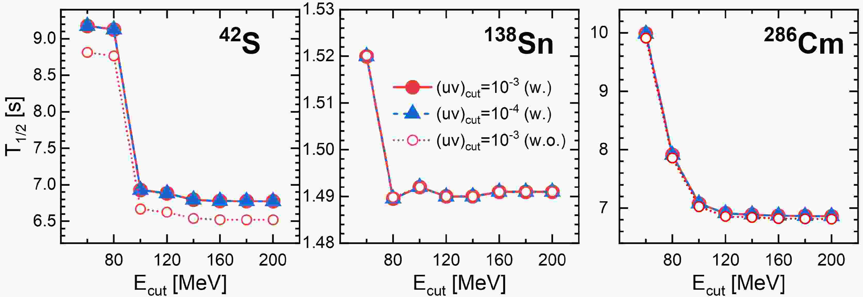
$ \beta^- $ -decay half-lives of three representative nuclei: 42S, 138Sn, and 286Cm. The two-quasiparticle energy cutoff$ E_{{\rm{cut}}} $ is varied from 60 to 200 MeV, and two cutoffs for the product of the occupation amplitudes,$ (uv)_{{\rm{cut}}}=10^{-3} $ and$ 10^{-4} $ , are considered. For$ (uv)_{{\rm{cut}}}=10^{-3} $ , calculations with and without Dirac-sea configurations are also performed to assess their impact on the calculated$ \beta^- $ -decay half-lives.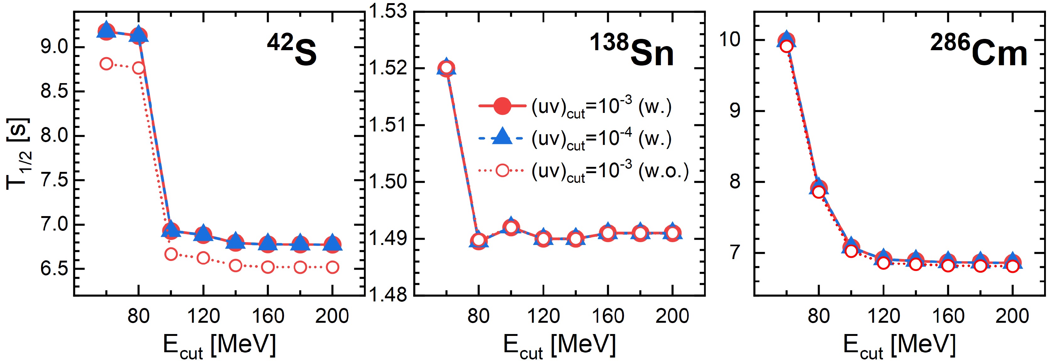
Figure 1. (color online) The β-decay half-lives of 42S, 138Sn, and 286Cm calculated by pnQRPA based on spherical RHFB theory with PCF-PK1, are plotted against
$ E_{{\rm{cut}}} $ . The results obtained with$ (uv)_{{\rm{cut}}}=10^{-3} $ and$ 10^{-4} $ are indicated by red circles and blue triangles, respectively, where Dirac sea is taken into account (w.). Open red circles denote calculations with$ (uv)_{{\rm{cut}}}=10^{-3} $ in which the Dirac-sea configurations are omitted (w.o.).For 42S, the calculated
$ \beta^- $ -decay half-life reaches a stable plateau as the two-quasiparticle energy cutoff$ E_{{\rm{cut}}} $ increases, with the results remaining nearly unchanged from$ E_{{\rm{cut}}}=100 $ to 200 MeV. The calculations performed with$ (uv)_{{\rm{cut}}}=10^{-3} $ and$ 10^{-4} $ yield very similar half-lives. In addition, omitting the Dirac-sea configurations changes the calculated half-life by only about 0.2 s, which is sufficiently small for the present calculations. For 138Sn, the half-life exhibits a plateau over the range$ E_{{\rm{cut}}}=120 $ –200 MeV. Although the result at$ E_{{\rm{cut}}}=100 $ MeV is already close to those obtained at higher cutoffs, a small deviation occurs between$ E_{{\rm{cut}}}=80 $ and 100 MeV. We therefore regard$ E_{{\rm{cut}}}=120 $ MeV as sufficient to achieve numerical stability. The calculated half-lives are essentially independent of whether$ (uv)_{{\rm{cut}}}=10^{-3} $ or$ 10^{-4} $ is used, while the inclusion of Dirac-sea configurations has a negligible effect on the calculated half-life. For 286Cm, a stable plateau is obtained for$ E_{{\rm{cut}}}=120 $ –200 MeV. The results show essentially no dependence on the choice of$ (uv)_{{\rm{cut}}} $ , and the contribution from Dirac-sea configurations is also negligible. Based on these convergence tests,$ E_{{\rm{cut}}}=100 $ MeV is adopted for nuclei in the light-mass region with$ Z\leq28 $ , while$ E_{{\rm{cut}}}=120 $ MeV is used for nuclei in the medium-heavy and heavy-mass regions with$ Z>28 $ . In all calculations,$ (uv)_{{\rm{cut}}}=10^{-3} $ is adopted. Since the Dirac-sea configurations have only a negligible impact on the calculated$ \beta^- $ -decay half-lives, they are omitted in the present systematic calculations to reduce the computational cost.It has been suggested in Refs. [18, 21] that a constant value of the isoscalar pairing strength
$ f_{{\rm{IS}}} $ may be insufficient to describe the β-decay half-lives of nuclei in different regions of the nuclear chart. We adopt the same ansatz as in Refs. [18, 21], introducing$ f_{{\rm{IS}}} $ as a function of$ N-Z $ ,$ \begin{aligned} f_{{\rm{IS}}} = V_1 + \frac{V_2}{1+ {{\rm{e}}}^{a+b (N-Z)}} \, , \end{aligned} $
(12) In the present work, the isoscalar pairing strength
$ f_{{\rm{IS}}} $ is determined by fitting the calculated β-decay half-lives to the available experimental data [8]. The fitting procedure includes only 58 even-even nuclei with$ 4\leq N-Z\leq 36 $ . In Fig. 2, the$ f_{{\rm{IS}}} $ values obtained by fitting the experimental data for these 58 nuclei are shown as open red circles. These values approximately follow the form of Eq. (12). The fit as a function of$ N-Z $ is shown by the blue line and yields a coefficient of determination of 0.844. The resulting parametrization is$ V_1=1.476 $ ,$ V_2=-0.372 $ ,$ a=-12.575 $ , and$ b=0.526 $ .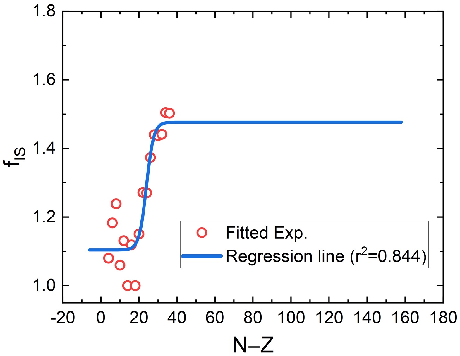
Figure 2. (color online) The isoscalar pairing strength
$f_{{\rm{IS}}} $ fitted to the experimental β-decay values of 58 even-even nuclei are plotted against$N-Z $ , denoting red open circles. The fitted isospin-dependent function is shown by the blue solid line, with a correlation coefficient of 0.844.For odd-A and odd-odd nuclei, the equal filling approximation (EFA) [30] is adopted in the ground-state calculation to account for the blocking effect. The occupation probabilities of the resulting ground state in the canonical basis are then used as input for the pnQRPA calculation, which is performed in the same way as for even-even nuclei.
-
To quantitatively assess the predictive performance of the different theoretical models, we compare their calculated β-decay half-lives with the available experimental data. For each nucleus, the logarithmic deviation between the theoretical and experimental half-lives and the average logarithmic deviation are defined as follows:
$ \begin{aligned} r_i = \log_{10} \left( \frac{T_{1/2,i}^{{\rm{th}}}} {T_{1/2,i}^{{\rm{exp}}}} \right), \quad \bar{r} = \frac{1}{N} \sum_{i=1}^{N} r_i \, , \end{aligned} $
(13) where
$ T_{1/2,i}^{{\rm{th}}} $ and$ T_{1/2,i}^{{\rm{exp}}} $ denote the calculated and experimental half-lives, respectively. The quantity$ \bar{r} $ characterizes the systematic bias of the model. A positive (negative) value of$ \bar{r} $ indicates that the theoretical half-lives tend to be overestimated (underestimated).The overall dispersion of the theoretical predictions around the experimental values is quantified by the standard deviation
$ \begin{aligned} \sigma = \left[ \frac{1}{N} \sum_{i=1}^{N} \left(r_i-\bar{r}\right)^2 \right]^{1/2}. \end{aligned} $
(14) A smaller σ therefore indicates a narrower distribution of the theoretical-to-experimental ratios and, consequently, better overall agreement with experiment. Because the comparison is performed on a logarithmic scale, σ can also be interpreted as a typical multiplicative deviation; that is, a value of σ corresponds approximately to a factor of
$ 10^\sigma $ in the half-life.In this work, both
$ \bar{r} $ and σ are evaluated and summarized in Table 1, enabling a quantitative comparison of the predictive capabilities of the different models. To ensure a fair comparison, we recalculate these quantities using the NUBASE2020 database [8]. The theoretical data are taken from the Supplemental Material of Refs. [12, 18], with only theoretical half-lives shorter than$ 10^{12} $ s included.PCF-PK1 (GT) D3C* (GT) D3C* (GT+FF) FRDM (GT+FF) $ \bar r $ σ $ \bar r $ σ $ \bar r $ σ $ \bar r $ σ Experimental range $<1000 $ s$ 0.409 $ $ 1.110 $ $ 0.344 $ $ 1.147 $ $ 0.202 $ $ 1.208 $ $ -0.028 $ $ 0.607 $ $<100 $ s$ 0.416 $ $ 1.054 $ $ 0.369 $ $ 1.031 $ $ 0.128 $ $ 0.920 $ $ -0.016 $ $ 0.541 $ $<10 $ s$ 0.365 $ $ 0.927 $ $ 0.352 $ $ 0.829 $ $ 0.133 $ $ 0.748 $ $ -0.031 $ $ 0.479 $ $<1 $ s$ 0.243 $ $ 0.707 $ $ 0.243 $ $ 0.467 $ $ 0.079 $ $ 0.454 $ $ -0.025 $ $ 0.390 $ $<0.1 $ s$ 0.148 $ $ 0.329 $ $ 0.245 $ $ 0.297 $ $ 0.130 $ $ 0.294 $ $ 0.025 $ $ 0.325 $ Nucleus type ( $ T_{1/2}^{{\rm{exp}}}<0.1 $ s)even-even $ 0.139 $ $ 0.269 $ $ 0.185 $ $ 0.285 $ $ 0.054 $ $ 0.258 $ $ 0.287 $ $ 0.204 $ odd-Z even-N $ 0.143 $ $ 0.302 $ $ 0.247 $ $ 0.216 $ $ 0.149 $ $ 0.226 $ $ -0.172 $ $ 0.232 $ odd-N even-Z $ 0.124 $ $ 0.271 $ $ 0.226 $ $ 0.268 $ $ 0.121 $ $ 0.222 $ $ 0.217 $ $ 0.306 $ odd-odd $ 0.180 $ $ 0.428 $ $ 0.315 $ $ 0.372 $ $ 0.189 $ $ 0.395 $ $ -0.156 $ $ 0.256 $ Table 1. The standard deviation σ and mean deviation
$ \bar{r} $ between the calculated and experimental data for nuclei with different ranges of half-lives [8], considering only nuclei with$ T_{1/2}^{{\rm{Cal.}}}<10^{12} $ s. In the upper panel, the spherical localized RHFB + pnQRPA results using PCF-PK1 are denoted by PCF-PK1 (GT). Results from RHB+pnQRPA calculations using D3C* without and with the inclusion of FF transitions [18], and FRDM + QRPA calculations with the inclusion of FF transitions [12] are also listed. In the lower panel, the results for nuclei with$ T_{1/2}^{{\rm{Exp.}}}<0.1 $ s are separated into even-even, odd-Z even-N, odd-N even-Z, and odd-odd nuclei.In the upper part of the table, for nuclei with
$ T_{1/2}^{{\rm{Exp.}}}<1000 $ s and 100 s, the standard deviations obtained with PCF-PK1 are comparable to those obtained with D3C*. However, for nuclei with$ T_{1/2}^{{\rm{Exp.}}}<1000 $ s, 678 nuclei are considered in the PCF-PK1 results, whereas 724 nuclei are considered in the D3C* case. For the common set of 661 nuclei with$ T_{1/2}^{{\rm{Exp.}}}<1000 $ s, the standard deviation obtained with PCF-PK1 is 1.049, slightly higher than the value of 0.987 obtained with D3C*. For nuclei with$ T_{1/2}^{{\rm{Exp.}}}<100 $ s, 639 nuclei are considered in the PCF-PK1 results, whereas 670 nuclei are considered in the D3C* case. For the common set of 627 nuclei with$ T_{1/2}^{{\rm{Exp.}}}<100 $ s, the standard deviation obtained with PCF-PK1 is 0.998, which is also slightly higher than the value of 0.930 obtained with D3C*. Compared with D3C* (GT), the σ values decrease when FF transitions are considered, except in the case of$ T_{1/2}^{{\rm{Exp.}}}<1000 $ s. However, this improvement is insufficient to bridge the gap between the self-consistent calculations and the FRDM+QRPA results. When both GT and FF transitions are considered, the σ values remain much lower in FRDM+QRPA than in the self-consistent calculations, except for nuclei with$ T_{1/2}^{{\rm{Exp.}}}<0.1 $ s, for which the PCF-PK1 result shows a σ value comparable to those of the D3C* and FRDM+QRPA results.For the average deviations, the PCF-PK1 result is higher than that of D3C* (GT) for nuclei with
$ T_{1/2}^{{\rm{Exp.}}}<1000 $ s and 100 s, but becomes nearly the same and even smaller in the other cases, indicating the potential of PCF-PK1 for nuclei with large$ Q_{\beta} $ values. When FF transitions are included, the average deviations are significantly reduced, yielding consistently lower$ \bar{r} $ values for D3C* (GT+FF) than for PCF-PK1. In the calculations with both PCF-PK1 and D3C*,$ \bar{r} $ has positive values, indicating that the β-decay half-lives are consistently overestimated. Including the FF contributions reduces the$ \bar{r} $ values, although they remain positive, suggesting that FF contributions mitigate the overestimation of half-lives. The FRDM+QRPA results yield much lower absolute$ \bar{r} $ values than the self-consistent results. In contrast to the positive$ \bar{r} $ values in the self-consistent calculations, the$ \bar{r} $ values are negative in most of the FRDM+QRPA calculations, indicating an underestimation of half-lives.The performances of different models for the β-decay half-lives of nuclei with
$ T_{1/2}^{{\rm{Exp.}}}<0.1 $ s are similar. Therefore, in the lower panel of the table, we further divide these nuclei into four groups for closer examination: even-even, odd-Z even-N, odd-N even-Z, and odd-odd nuclei. The performance differs considerably among these groups. In the self-consistent calculations, the σ values for odd-odd nuclei are higher than those for the other groups, whereas in the FRDM+QRPA calculations, the σ values for odd-N nuclei are higher. This suggests that the treatment of odd nuclei in these works is overly simplified and should be implemented in a more self-consistent manner, as in Refs. [14, 19].Regarding the average deviation, the self-consistent calculations generally yield better results than FRDM+QRPA, and among the self-consistent calculations, PCF-PK1 performs better than D3C* (GT). It is also noteworthy that the self-consistent results differ considerably from the FRDM+QRPA results. The self-consistent calculations yield positive
$ \bar{r} $ values for all types of nuclei. For example, for odd-odd nuclei, PCF-PK1 overestimates by 50%, whereas D3C*(GT) overestimates by about 100%. In contrast, the FRDM+QRPA results show positive$ \bar{r} $ values for even-even and odd-N nuclei but negative values for the other groups. This contrasting behavior among different types of nuclei in the FRDM+QRPA calculations explains why FRDM+QRPA yields a much smaller$ \bar{r} $ while giving a σ value comparable to that of the self-consistent calculations, as a result of the cancellation between overestimations and underestimations. Moreover, the$ \bar{r} $ values in the D3C* (GT+FF) results are smaller than those in the D3C* (GT) case, suggesting that the inclusion of FF transitions reduces the average deviations for all types of nuclei.In Fig. 3, we display the logarithmic deviations of the calculated half-lives with respect to experiment as a function of
$ T_{1/2}^{{\rm{Exp.}}} $ , where nuclei with$ T_{1/2}^{{\rm{Exp.}}}<1000 $ s are separated into even-even, odd-A, and odd-odd nuclei. The PCF-PK1 results, denoted by orange symbols, are compared with those of D3C*, denoted by blue symbols.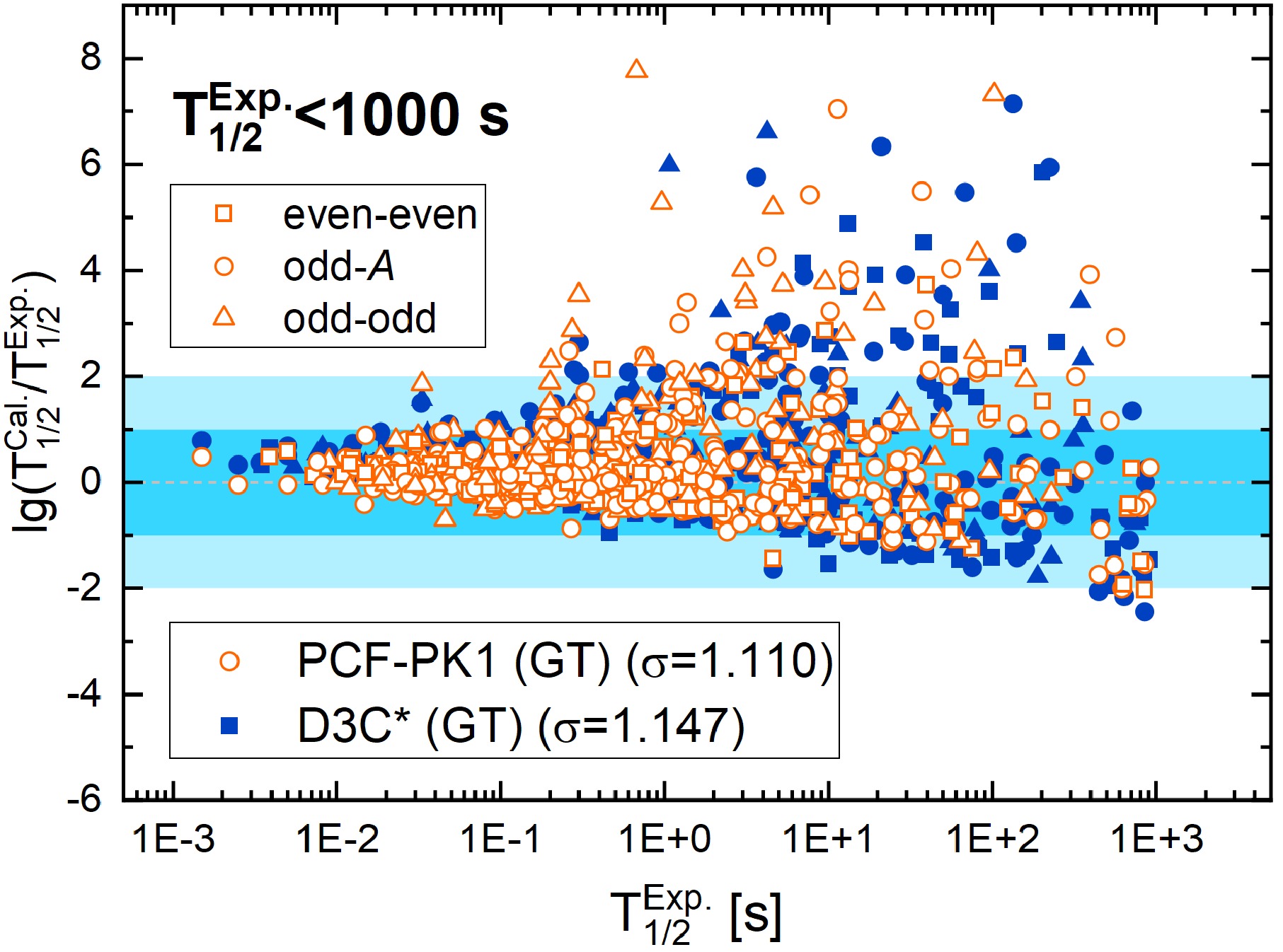
Figure 3. (color online) The logarithmic deviations of the spherical pnQRPA (allowed GT approximation) calculations using PCF-PK1 (open orange symbols) and D3C* (solid blue symbols) for nuclei with
$T_{1/2}^{{\rm{Exp.}}}<1000 $ s are plotted against the experimental data, where nuclei are separated into even-even (squares), odd-A (circles), and odd-odd (triangles) nuclei. The light and deep blue shadow represent the deviation within one and two orders, respectively.Most nuclei lie within the shaded bands: approximately 80% have half-life ratios within one order of magnitude, and 90% are within two orders of magnitude. Large spreads in the half-life ratios are found for long-lived nuclei, whose calculated half-lives are more sensitive to the details of the β-decay strength distribution because of the small β-decay window. In contrast, the broader decay window for short-lived nuclei allows contributions from a wider range of transition strengths. In this regime, the total transition strength, rather than its detailed distribution, is more important, leading to a more robust description of the half-lives. In both the PCF-PK1 and D3C* calculations, the half-life ratios tend to fall within one order of magnitude with decreasing
$ T_{1/2}^{{\rm{Exp.}}} $ for all types of nuclei, indicating good agreement between the calculated and experimental half-lives across different types of nuclei in the short-lived region.The odd-A and odd-odd nuclei contribute substantially to the spread of the ratios for long-lived nuclei. Fifty-five nuclei lie outside the lightly shaded region in the PCF-PK1 calculations, and 57 nuclei do so in the D3C* calculations; most of these nuclei have half-lives longer than 1 s. Among them, even-even, odd-A, and odd-odd nuclei account for 16%, 45%, and 38% in the PCF-PK1 calculations, compared with 21%, 49%, and 30% in the D3C* results. Although the D3C* calculations include more even-even nuclei than the PCF-PK1 calculations, both calculations show that the nuclei with large deviations from the experimental data are predominantly odd-A and odd-odd nuclei, indicating that the treatment of odd nuclei requires improvement, as discussed in Table 1.
To obtain a more detailed view, Fig. 4 shows the logarithmic deviations from the experiment [8] across the nuclear chart. The spherical RHFB+pnQRPA calculations under the allowed GT approximation using the PCF-PK1 and D3C* results [18] are shown in panels (a) and (b), respectively.
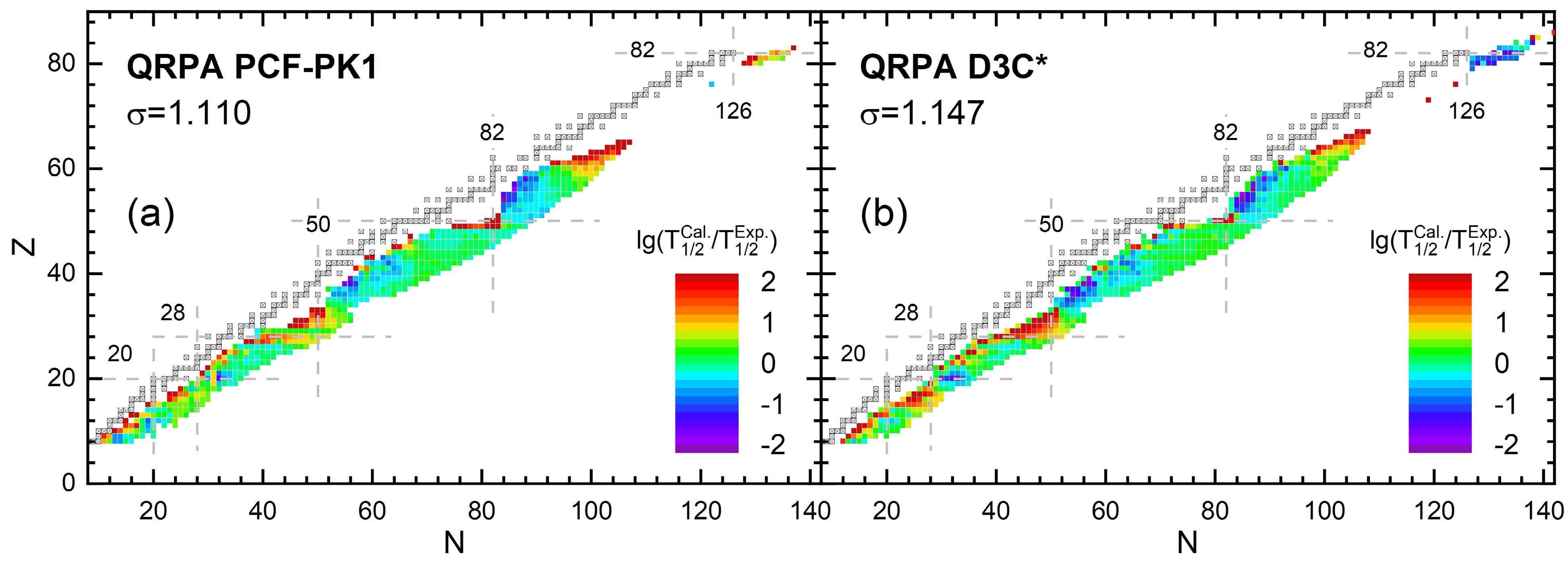
Figure 4. (color online) The logarithmic deviations of the spherical RHFB+pnQRPA (allowed GT approximation) calculations using PCF-PK1 (a) and D3C* (b) [18] with respect to the experiment [8] are scaled by colors, where nuclei with
$ T_{1/2}^{{\rm{Exp.}}}<1000 $ s are considered. The stable nuclei are shown by squares with cross. Magic numbers are denoted by dashed grey lines.Notably, both the PCF-PK1 and D3C* results exhibit small deviations for nuclei far from the valley of stability but large deviations for nuclei near the β-stability line and around magic numbers. This trend is consistent with Fig. 3, because nuclei far from the valley of stability have shorter half-lives, whereas those closer to the β-stability line have longer half-lives.
For the PCF-PK1 results, the overestimation of β-decay half-lives is concentrated around the magic numbers
$ Z=28, 50, 82 $ and$ N=50 $ , as well as in the mid-shell region around$ (Z=65, N=106) $ , as shown in panel (a). For D3C*, substantial overestimations also appear around magic numbers such as$ Z=28, 50 $ and$ N=50 $ , as well as in a similar mid-shell region. However, overestimations remain between$ N=20 $ and$ 30 $ and in the northwest region of$ ^{78} $ Ni. In contrast, the overestimation in the$ Z=82 $ region for PCF-PK1 becomes an underestimation for D3C*. The overestimation around magic numbers could be reduced by including correlations beyond the QRPA approach, such as coupling to collective phonon excitations, as demonstrated in Refs. [31−34]. The overestimation in the mid-shell region could be reduced by including FF transitions and deformation effects. According to the GT+FF calculations using D3C*, this overestimation is reduced when FF contributions are introduced [18]. In addition, the nuclei in this region are well deformed, and their β-decay half-lives can be sensitive to nuclear deformation [35−38]. In addition to the overestimation, apparent underestimations also occur in the mid-shell region between$ Z=28 $ and 50, as well as in the northeast corner of 132Sn, for both PCF-PK1 and D3C*. The underestimation is more pronounced for D3C* than for PCF-PK1.In addition to nuclei with experimental data, theoretical models also predict
$ \beta^- $ -decay half-lives for nuclei without experimental data. For example, the present work using PCF-PK1 predicts half-lives for 5456 nuclei located on the right side of the β-stability line with$ 8\leq Z\leq120 $ , whereas the corresponding numbers are 5409 and 6070 for RHB+pnQRPA (D3C*) and FRDM+QRPA, respectively. Therefore, we further compare the β-decay half-lives predicted in the present work with those of other models in Fig. 5. The comparisons with spherical RHB+pnQRPA (GT) calculations using D3C* [18] and FRDM+QRPA (GT+FF) calculations [12] are shown in panel (a) and panel (b) of Fig. 5, respectively. Note that nuclei predicted to be stable in both calculations are excluded from the comparison.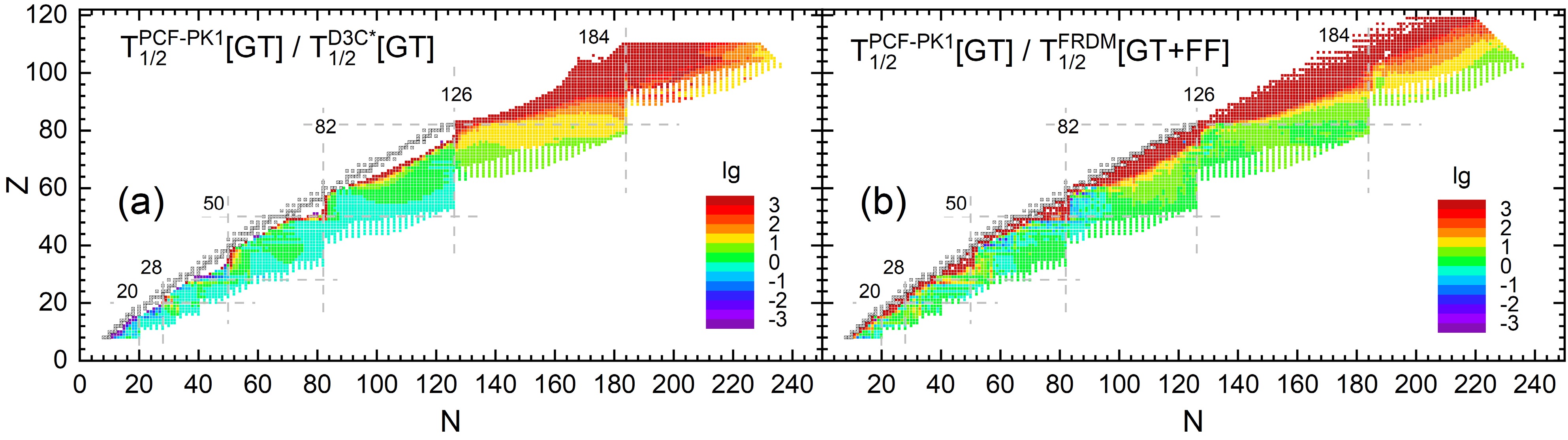
Figure 5. (color online) The logarithmic difference between the RHFB+pnQRPA (GT) calculations using PCF-PK1 and other models, including (a) the RHB+pnQRPA (GT) results using D3C* [18], and (b) the FRDM+QRPA (GT+FF) results [12]. The stable nuclei are shown by squares with cross. Magic numbers are denoted by dashed grey lines.
In panel (a), the differences between the two models are modest for most light and medium-heavy nuclei, with logarithmic deviations within one order of magnitude. For heavy nuclei around
$ Z=82 $ , PCF-PK1 systematically overestimates the half-lives relative to D3C* over the entire isotopic chain by about 1–2 orders of magnitude. For heavier nuclei with$ Z>82 $ and$ N>126 $ , the half-lives predicted in the present work are about 3 orders of magnitude longer than those of D3C*. This behavior may be due to the large isoscalar pairing strength used in D3C*. These heavy-nucleus regions still lack experimental data. In lighter nuclear regions where experimental data are available, PCF-PK1 overestimates the half-lives relative to D3C* for nuclei close to the β-stability line between$ Z=61 $ and 82, along the$ N=83 $ isotonic chain with$ Z \geq 49 $ , and along the$ Z=49 $ isotopic chain with$ N\leq 83 $ . In all three regions, D3C* is correspondingly closer to experiment, with σ values of 0.98, 0.19, and 0.15 orders of magnitude, respectively, whereas those of PCF-PK1 are 1.49, 2.36, and 0.65. In addition to these overestimations, PCF-PK1 also underestimates the half-lives relative to D3C* for nuclei along the$ Z=29 $ isotopic chain with$ N\leq 50 $ and in the light nuclear region close to the β-stability line with$ Z \lt 20 $ . In these two regions, PCF-PK1 is closer to experiment, with$ \sigma=0.049 $ and 0.904, compared with 0.878 and 1.920 for D3C*, respectively. We note that these large deviations occur either in nuclei close to the β-stability line or in odd nuclei near magic numbers. Therefore, after the inclusion of the self-consistent treatment of odd nuclei and correlations beyond QRPA, these two approaches may converge to more similar results.In panel (b), the comparison between PCF-PK1 and FRDM+QRPA exhibits a clearly different pattern from that between PCF-PK1 and D3C* in panel (a). Here, systematic overestimations for nuclei near the β-stability line occur across the entire nuclear chart. In particular, in panel (a), there are some blank regions very close to the β-stability line because these nuclei are predicted to be stable in both PCF-PK1 and D3C* calculations and are therefore excluded. However, these nuclei are predicted to have finite half-lives in FRDM+QRPA, and thus they are still shown in panel (b). Apart from these severe overestimations near the β-stability line, PCF-PK1 gives results more similar to those of FRDM+QRPA. The deviations are generally within one order of magnitude. In particular, for nuclei with
$ Z>74 $ , PCF-PK1 shows results similar to those of FRDM+QRPA as one moves toward the neutron-rich region, in contrast to the strong overestimation relative to the D3C* results. The large deviation of odd nuclei near magic numbers in the comparison with the D3C* results also disappears here, indicating a more similar treatment of odd nuclei in PCF-PK1 and FRDM+QRPA.To examine the performance of RHFB+pnQRPA calculations with PCF-PK1 more closely, we display in Fig. 6 the calculated β-decay half-lives for the Cu (
$ Z=29 $ ), Pd ($ Z=46 $ ),$ N=18 $ , and$ N=35 $ isotopic or isotonic chains, obtained from spherical RHFB+pnQRPA calculations using PCF-PK1 (red stars), together with the PCF-PK1 results with$ f_{{\rm{IS}}}=0 $ (green triangles) and the D3C* (GT) results [18] (blue circles). The experimental data [8] are plotted as black squares for comparison.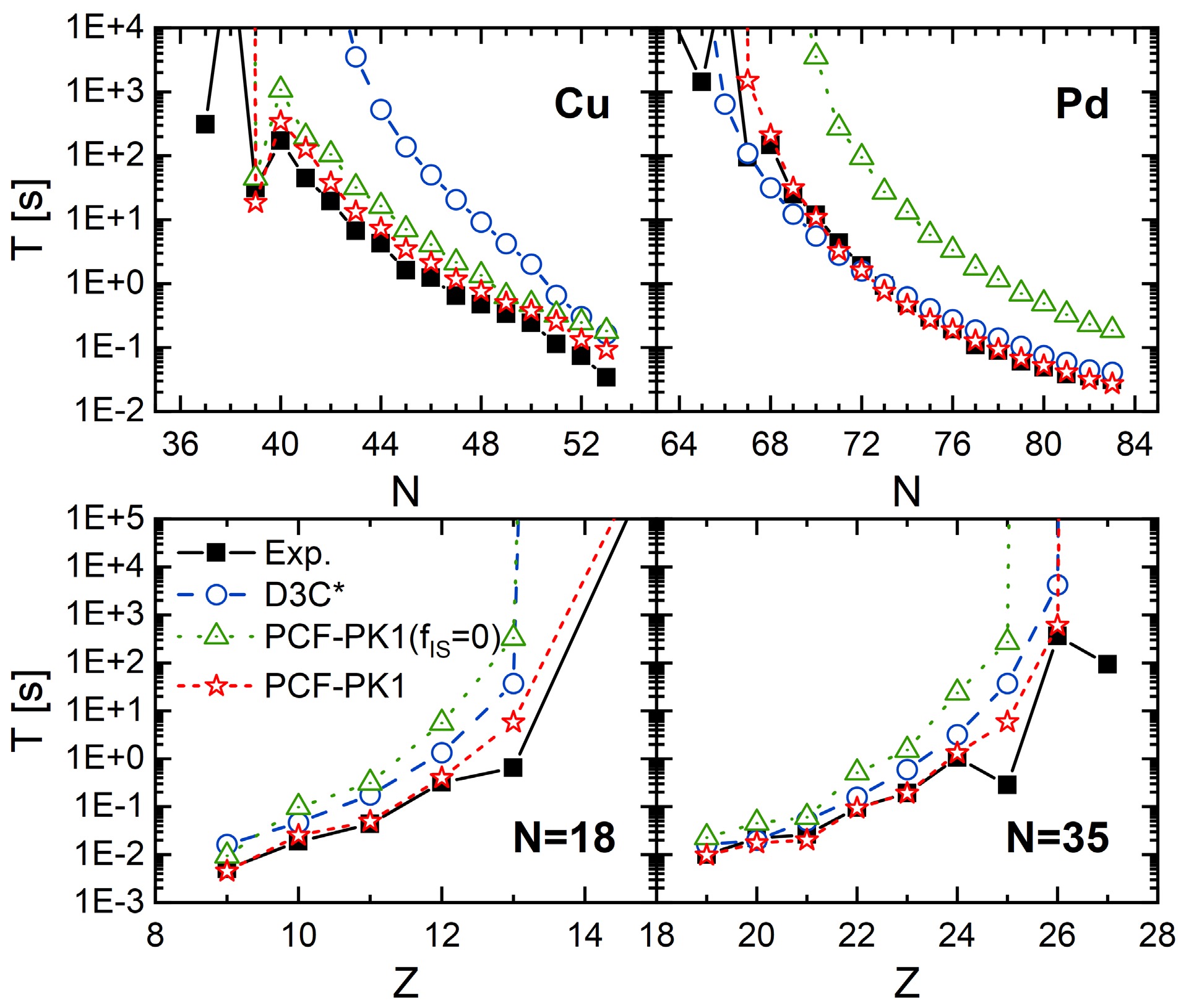
Figure 6. (color online) The β-decay half-lives for the Cu (
$Z=29 $ ), Pd ($Z=46 $ ),$ N=18$ , and$N=35 $ chains, are obtained from spherical RHFB+pnQRPA (GT) calculations using PCF-PK1 (red stars), together with the case of$f_{{\rm{IS}}}=0 $ (green triangles), and from RHB+pnQRPA (GT) calculations using D3C* (blue circles) [18]. The experimental data (black squares) [8] are shown for comparison.For the Cu isotopes, PCF-PK1 reproduces the experimental isotopic trend of the half-lives over the entire chain. In particular, the kink at
$ N=39 $ is consistently reproduced in calculations with both$ f_{{\rm{IS}}}=0 $ and the isospin-dependent$ f_{{\rm{IS}}} $ . The isospin-dependent isoscalar pairing strength varies between$ f_{{\rm{IS}}}=1.10 $ and 1.29, and the effect of isoscalar pairing is very small for this isotopic chain. Therefore, the inclusion of$ f_{{\rm{IS}}} $ only slightly reduces the half-lives and leads to better agreement with experiment. In contrast, the D3C* results overestimate the half-lives over a broad range, from the stability valley toward the neutron drip line. Since the half-lives are not very sensitive to the isoscalar pairing strength, the difference between these two calculations may arise from the relatively smaller Landau effective mass$ M_L^* $ of D3C*. For nuclei with large$ Q_\beta $ values, the D3C* predictions gradually approach those of PCF-PK1, although they remain systematically longer.For the Pd isotopes, the PCF-PK1 calculations with
$ f_{{\rm{IS}}}=0 $ overestimate the half-lives by about an order of magnitude. The inclusion of the isospin-dependent$ f_{{\rm{IS}}} $ substantially reduces this discrepancy and brings the calculated half-lives into much better agreement with experiment. Both PCF-PK1 and D3C* follow the trend of the half-lives along the isotopic chain, with PCF-PK1 providing better agreement with the experimental data for most nuclei.For the
$ N=18 $ and$ N=35 $ isotonic chains, the PCF-PK1 calculation with$ f_{{\rm{IS}}}=0 $ increasingly overestimates the half-lives toward the stability valley. The inclusion of the isospin-dependent$ f_{{\rm{IS}}} $ substantially reduces the deviations and yields good agreement with experiment, except for the kinks at$ Z=13 $ in the$ N=18 $ isotonic chain and at$ Z=25 $ in the$ N=35 $ isotonic chain. The D3C* results lie between the two PCF-PK1 calculations and tend to overestimate the experimental values. -
The RHFB+pnQRPA calculations with PCF-PK1 provide a systematic description of nuclear β-decay half-lives, with a standard deviation of
$ \sigma=1.110 $ relative to experimental data. Although this level of accuracy is useful for global studies, theoretical uncertainties of this magnitude can lead to variations of roughly one order of magnitude in the predicted r-process abundance pattern [5]. Further improvements in β-decay half-lives are therefore highly desirable. To reduce this uncertainty, we exploit the strong correlations in β-decay properties among neighboring nuclei along isotopic and isotonic chains. Such sequential correlations are well suited to recurrent neural networks (RNNs). In particular, the gated recurrent unit (GRU), which extends a standard RNN by introducing update and reset gates to regulate the retention and updating of historical information, has recently been applied to the prediction of nuclear binding energies [39]. We therefore adopt a GRU network to learn these correlations and improve the predicted logarithmic β-decay half-lives relative to the RHFB+pnQRPA results.In this work, nuclei are organized as ordered sequences along isotopic and isotonic chains, and two independent GRU branches are constructed to learn correlations among neighboring nuclei along the neutron-number (N) and proton-number (Z) directions, respectively. Each nucleus is represented by five physical quantities,
$ \begin{aligned} {\boldsymbol{x}} = \left( Z,\, N,\, \lg Q_\beta,\, \delta,\, \lg T_{{\rm{th}}} \right). \end{aligned} $
(15) Here, Z and N denote the proton and neutron numbers, respectively. The
$ Q_\beta $ value of β decay is calculated from the mass excesses of the parent nucleus$ (Z,N) $ and daughter nucleus$ (Z+1,N-1) $ as$ Q_\beta=M(Z,N)- M(Z+1,N-1) $ , where M denotes the nuclear mass excess. This value is obtained from the Bayesian machine-learning mass model with an accuracy of 84 keV [40]. The odd-even property is characterized by$ \delta=[(-1)^Z+(-1)^N]/2 $ , which takes the values$ 1 $ ,$ -1 $ , and$ 0 $ for even-even, odd-odd, and odd-A nuclei, respectively.$ T_{{\rm{th}}} $ denotes the theoretical β-decay half-life calculated using the localized RHFB+pnQRPA model with the PCF-PK1 interaction. Accordingly, the extrapolation region of the neural network is restricted to the intersection of the nuclear charts covered by the$ Q_\beta $ values and the PCF-PK1 half-life calculations. The logarithmic quantities$ \lg Q_\beta $ and$ \lg T_{{\rm{th}}} $ are used as network inputs, while the prediction target is the experimental logarithmic half-life$ \lg T_{1/2} $ .The experimental β-decay data are taken from NUBASE2020 [8]. The dataset includes nuclei with
$ Z>8 $ and$ N>8 $ , experimental β-decay half-lives shorter than$ 10^{6} $ s, and β-decay branching ratios greater than 10%. After these selection criteria are applied, the nuclei are arranged according to their positions along the isotopic chains. The dataset is then divided into training and validation sets: the first four nuclei of each isotopic chain are always assigned to the training set, and approximately 25% of the remaining nuclei are randomly selected for validation. Finally, the training and validation sets contain 802 and 267 nuclei, respectively.The architecture of the proposed GRU framework is shown in Fig. 7. The upper and lower branches extract sequential correlations along the N and Z directions, respectively. Each branch consists of a GRU layer with 8 hidden units, followed by a fully connected layer with 12 neurons and the Tanh activation function. Two output layers are then used to generate the half-life prediction and the corresponding decreasing quantity. After the directional constraint is imposed, the information learned from the two directions is combined to obtain the final prediction.
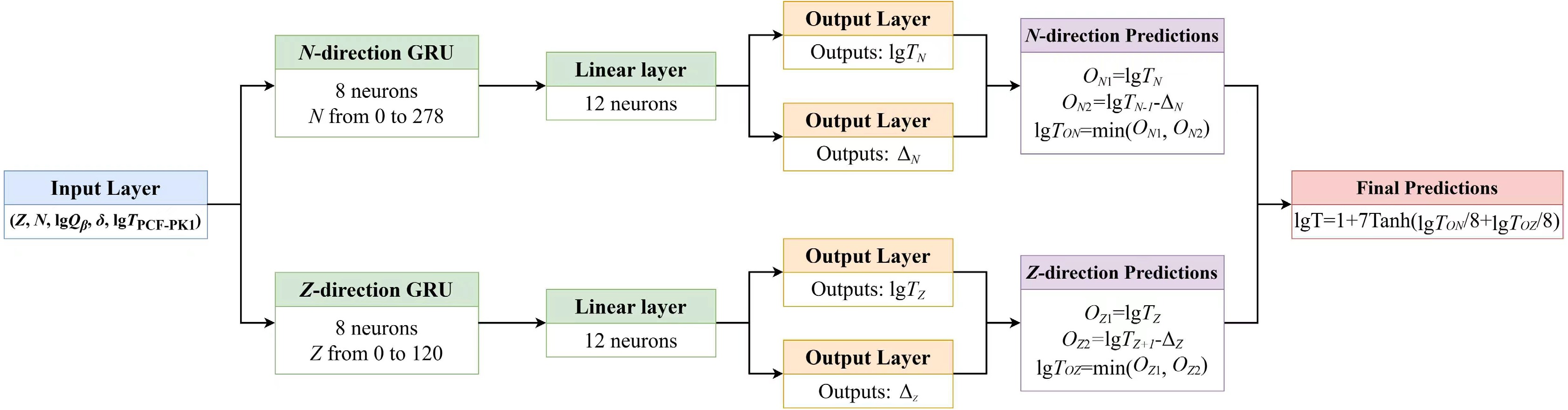
Figure 7. (color online) Schematic illustration of the proposed GRU framework for β-decay half-life prediction. The two GRU branches extract the sequential correlations along the neutron-number (N) and proton-number (Z) directions, respectively. Each branch generates the logarithmic half-life and the corresponding decreasing quantity, and the directional constraints are imposed before combining the two branches to obtain the final prediction.
For an N-direction GRU, the recurrent propagation is expressed as
$ \begin{aligned}[b] {\boldsymbol{r}}_{N} &= \sigma\left({\boldsymbol{W}}_{r,N}{\boldsymbol{x}}+{\boldsymbol{U}}_{r,N}{\boldsymbol{h}}_{N-1}^{(1)}+{\boldsymbol{b}}_{r,N}\right),\\ {\boldsymbol{z}}_{N} &= \sigma\left({\boldsymbol{W}}_{z,N}{\boldsymbol{x}}+{\boldsymbol{U}}_{z,N}{\boldsymbol{h}}_{N-1}^{(1)}+{\boldsymbol{b}}_{z,N}\right),\\ \widetilde{{\boldsymbol{h}}}_{N} &= \tanh\left[{\boldsymbol{W}}_{h,N}{\boldsymbol{x}}+{\boldsymbol{U}}_{h,N}\left({\boldsymbol{r}}_{N}\odot{\boldsymbol{h}}_{N-1}^{(1)}\right)+{\boldsymbol{b}}_{h,N}\right],\\ {\boldsymbol{h}}_{N}^{(1)} &= \left(1-{\boldsymbol{z}}_{N}\right)\odot{\boldsymbol{h}}_{N-1}^{(1)}+{\boldsymbol{z}}_{N}\odot\widetilde{{\boldsymbol{h}}}_{N}. \end{aligned} $
(16) Here,
$ {\boldsymbol{r}}_{N} $ and$ {\boldsymbol{z}}_{N} $ denote the reset and update gates, respectively; σ is the sigmoid activation function; and$ \odot $ denotes element-wise multiplication.$ {\boldsymbol{W}} $ and$ {\boldsymbol{U}} $ denote the input and recurrent weight matrices, respectively, and$ {\boldsymbol{b}} $ denotes the bias vector.$ \widetilde{{\boldsymbol{h}}} $ and$ {\boldsymbol{h}} $ represent the candidate and updated hidden states, respectively. The subscript N denotes the neutron-number direction, while r, z, and h distinguish the reset gate, update gate, and hidden-state-related parameters.The Z-direction GRU follows the same structure,
$ \begin{aligned}[b] {\boldsymbol{r}}_{Z} &= \sigma\left({\boldsymbol{W}}_{r,Z}{\boldsymbol{x}}+{\boldsymbol{U}}_{r,Z}{\boldsymbol{h}}_{Z-1}^{(1)}+{\boldsymbol{b}}_{r,Z}\right),\\ {\boldsymbol{z}}_{Z} &= \sigma\left({\boldsymbol{W}}_{z,Z}{\boldsymbol{x}}+{\boldsymbol{U}}_{z,Z}{\boldsymbol{h}}_{Z-1}^{(1)}+{\boldsymbol{b}}_{z,Z}\right),\\ \widetilde{{\boldsymbol{h}}}_{Z} &= \tanh\left[{\boldsymbol{W}}_{h,Z}{\boldsymbol{x}}+{\boldsymbol{U}}_{h,Z}\left({\boldsymbol{r}}_{Z}\odot{\boldsymbol{h}}_{Z-1}^{(1)}\right)+{\boldsymbol{b}}_{h,Z}\right],\\ {\boldsymbol{h}}_{Z}^{(1)} &= \left(1-{\boldsymbol{z}}_{Z}\right)\odot{\boldsymbol{h}}_{Z-1}^{(1)}+{\boldsymbol{z}}_{Z}\odot\widetilde{{\boldsymbol{h}}}_{Z}. \end{aligned} $
(17) The GRU outputs are then mapped using fully connected layers.
$ \begin{aligned}[b] {\boldsymbol{h}}_{N}^{(2)} &= \tanh\left({\boldsymbol{w}}_{N}^{(2)}{\boldsymbol{h}}_{N}^{(1)}+{\boldsymbol{b}}_{N}^{(2)}\right),\\ {\boldsymbol{h}}_{Z}^{(2)} &= \tanh\left({\boldsymbol{w}}_{Z}^{(2)}{\boldsymbol{h}}_{Z}^{(1)}+{\boldsymbol{b}}_{Z}^{(2)}\right). \end{aligned} $
(18) For each direction, two independent output layers are introduced: one directly generates the logarithmic half-life, and the other generates the corresponding decreasing quantity.
$ \begin{aligned}[b] \lg T_{N} &= {\boldsymbol{w}}_{N}^{(3)}{\boldsymbol{h}}_{N}^{(2)}+b_{N}^{(3)}, & \Delta_{N} &= {\rm{Softplus}}\left({\boldsymbol{w}}_{N}^{(4)}{\boldsymbol{h}}_{N}^{(2)}+b_{N}^{(4)}\right),\\ \lg T_{Z} &= {\boldsymbol{w}}_{Z}^{(3)}{\boldsymbol{h}}_{Z}^{(2)}+b_{Z}^{(3)}, & \Delta_{Z} &= {\rm{Softplus}}\left({\boldsymbol{w}}_{Z}^{(4)}{\boldsymbol{h}}_{Z}^{(2)}+b_{Z}^{(4)}\right). \end{aligned} $
(19) Here,
$ {\boldsymbol{w}} $ and$ {\boldsymbol{b}} $ denote the weights and biases of the fully connected and output layers, respectively, and the superscripts indicate the corresponding layer indices.$ {\boldsymbol{h}}^{(1)} $ denotes the hidden state produced by the GRU layer, whereas$ {\boldsymbol{h}}^{(2)} $ denotes the hidden representation after the fully connected layer.$ \lg T_{N} $ and$ \lg T_{Z} $ denote the logarithmic half-life predictions from the N- and Z-direction branches, respectively, whereas$ \Delta_{N} $ and$ \Delta_{Z} $ represent the corresponding decreasing quantities. The Softplus activation function ensures that$ \Delta_{N} $ and$ \Delta_{Z} $ remain non-negative. For short-lived nuclei far from the stability line, the β-decay half-life generally decreases as nuclei move farther from stability, primarily because the increasing decay energy enlarges the available β-decay phase space. However, during extrapolation to experimentally unknown nuclei, an unconstrained neural network may produce unphysical increases in the predicted half-lives. Therefore, decreasing quantities are introduced to constrain the extrapolation behavior and preserve the physically expected trend.The directional constraints are then defined as
$ \begin{aligned}[b] \lg T_{N} &= \min\left(\lg T_{N},\ \lg T_{N-1}-\Delta_{N}\right),\\ \lg T_{Z} &= \min\left(\lg T_{Z},\ \lg T_{Z+1}-\Delta_{Z}\right). \end{aligned} $
(20) The constraints are activated only when the predicted half-life falls within the short-lived regime (
$ T<1 $ s); otherwise, the direct predictions of$ \lg T_{N} $ and$ \lg T_{Z} $ are retained.Finally, the two directional predictions are assigned equal weights and transformed using a scaled Tanh function,
$ \begin{aligned} \lg T = 1 + 7\tanh\left[\frac{\lg T_{N}+\lg T_{Z}}{8}\right]. \end{aligned} $
(21) The denominator, 8, contains two contributions. The factor 2 corresponds to the equal-weight averaging of the N- and Z-direction predictions, whereas the factor 4 controls the scale of the input to the Tanh function, preventing excessively rapid saturation and retaining sensitivity over the relevant prediction range. The constants 1 and 7 map the output of the Tanh function from
$ (-1,1) $ to approximately$ (-6,8) $ , covering the logarithmic range of the β-decay half-lives considered in the present work.Because the physical constraints are imposed separately on the two directional branches rather than directly on the final output, their combination does not necessarily guarantee strict monotonicity along both isotopic and isotonic chains. These constraints guide the network toward the overall systematic behavior of nuclear half-lives while allowing local nonmonotonic variations in the final predictions, because similar variations may also occur in experimental data. For neighboring pairs in which both nuclei have experimental data and the predicted half-lives are less than 1 s, the predictions satisfy the isotopic- and isotonic-chain constraints in 97.60% and 94.67% of cases, respectively. Among the pairs that violate these constraints, 70.83% agree with the experimental trend, leaving only seven pairs that both violate the constraints and disagree with the experimental trends. Among these seven pairs, six have longer predicted half-lives on the even-numbered side than on the odd-numbered side with respect to the varying nucleon number. The only exception is the 37Al~38Al pair, for which the predicted logarithmic half-life increases by only 0.00594. This slight deviation may be associated with local nonmonotonic features in the Al isotopic chain, as also observed in the experimental half-lives of 32Al~33Al and 35Al~36Al.
The sequence ranges are fixed at
$ 0\leq N\leq278 $ and$ 0\leq Z\leq120 $ , so that nuclei are represented at fixed positions along the corresponding isotopic and isotonic chains. The neural network is independently trained 1000 times to reduce the influence of random initialization. Considering both the predictive accuracy for experimental data and the systematic trends of the predicted half-lives, we selected 10 runs and adopted equal-weight averaging to obtain the final predictions.Fig. 8 compares the deviations between the predicted and experimental β-decay half-lives obtained with GRU, FRDM, and PCF-PK1. The red, blue, and green symbols correspond to GRU, FRDM, and PCF-PK1, respectively. Panels (a) and (b) show the results for the training and validation sets.
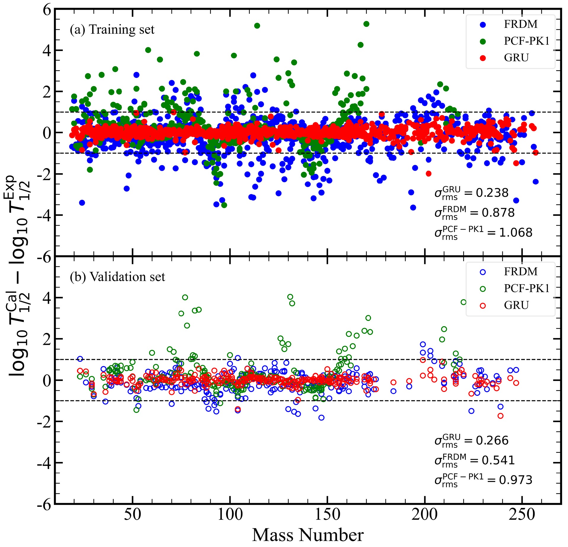
Figure 8. (color online) Deviations between the predicted and experimental β-decay half-lives for the training and validation sets. Panels (a) and (b) correspond to the training and validation sets, respectively. The red, blue, and green symbols denote the results obtained with GRU, FRDM, and PCF-PK1, respectively. The dashed horizontal lines indicate deviations of ±1 order of magnitude. The corresponding σ are also given in each panel.
For the training set, according to Eq. (14), the standard deviations of GRU, FRDM, and PCF-PK1 are 0.238, 0.878, and 1.068 orders of magnitude, respectively. For the validation set, the corresponding σ values are 0.266, 0.541, and 0.973 orders of magnitude.
Considering all nuclei, the overall standard deviations are 0.245 and 0.807 orders of magnitude for GRU and FRDM, respectively. For PCF-PK1, only the 690 nuclei with calculated half-lives shorter than
$ 10^{6} $ s are included, yielding an overall standard deviation of 1.038 orders of magnitude. For this common set of 690 nuclei, GRU gives$ \sigma=0.171 $ . Thus, GRU reduces the overall standard deviation by 69.6% and 83.6% relative to FRDM and PCF-PK1, respectively.During dataset splitting, the first four nuclei of each isotopic chain are always retained in the training set and excluded from the validation set. These nuclei are mainly located in the long-lived region near stability, where the FRDM and PCF-PK1 calculations show relatively large deviations. Consequently, the σ values of FRDM and PCF-PK1 are larger for the training set than for the validation set. Even under this condition, GRU reduces σ by approximately 72.8% and 87.0% relative to FRDM and PCF-PK1, respectively, for the training set, and by approximately 50.9% and 77.1% for the validation set.
As shown in Fig. 8, the deviations of the GRU predictions are more strongly concentrated around zero and exhibit a noticeably narrower distribution than those of FRDM and PCF-PK1. Taking a deviation larger than one order of magnitude as the criterion for a large prediction error, only 2 of the 802 training nuclei and 2 of the 267 validation nuclei exceed this range for GRU, corresponding to 0.25% and 0.75%, respectively. In comparison, FRDM gives deviations larger than one order of magnitude for 152 training nuclei and 23 validation nuclei, corresponding to 18.95% and 8.61%, respectively. For PCF-PK1, some long-lived nuclei are predicted to be stable. Therefore, only nuclei with PCF-PK1 half-lives shorter than
$ 10^{6} $ s are included in the statistical comparison. After this selection, 468 training nuclei and 222 validation nuclei remain. Among them, 107 training nuclei and 37 validation nuclei have deviations larger than one order of magnitude, corresponding to 22.86% and 16.67%, respectively.A nucleus-by-nucleus comparison further shows that the GRU prediction is closer to the experimental value than the FRDM result for 773 of the 802 training nuclei, corresponding to 96.38%, and for 241 of the 267 validation nuclei, corresponding to 90.26%. This indicates that the improvement obtained with GRU is not dominated by a small number of nuclei but is observed systematically across most of the dataset.
-
We performed systematic calculations of
$ \beta^- $ -decay half-lives for 5456 nuclei with$ 8\leq Z\leq 120 $ , covering even-even, odd-A, and odd-odd nuclei, within the localized RHFB + pnQRPA framework using the point-coupling functional PCF-PK1. The Fierz transformation localizes the exchange terms, so that every channel of the particle-hole residual interaction, including the isovector-pseudovector channel, is fixed by the ground state rather than adjusted phenomenologically. In addition, the isoscalar tensor coupling increases the Landau effective mass to$ M_L^*=0.85M $ . The spherical and allowed GT approximations are adopted, blocking in odd-A nuclei is treated by EFA, and the isoscalar proton-neutron pairing strength$ f_{{\rm{IS}}}(N-Z) $ is fitted to the measured half-lives of 58 even-even nuclei.The predictive accuracy depends on the experimental half-life range. For
$ T_{1/2}^{{\rm{Exp.}}}<1000 $ s, the σ values obtained with PCF-PK1 and D3C*(GT) are comparable, and both the standard deviation σ and the average deviation$ \bar r $ decrease as the experimental half-life shortens. For$ T_{1/2}^{{\rm{Exp.}}}<0.1 $ s, PCF-PK1 reaches$ \sigma=0.329 $ , comparable to the values obtained with the D3C* and FRDM+QRPA calculations. The self-consistent results yield positive$ \bar r $ , indicating a systematic overestimation of the half-lives.Analysis of the deviations from experiment shows that large overestimations occur around the magic numbers, suggesting that correlations beyond the QRPA need to be included, and in the deformed mid-shell region near
$ (Z=65,N=106) $ , where deformation and FF transitions are expected to be important. The largest deviations in the self-consistent calculations occur for odd-odd nuclei, indicating that a more self-consistent treatment of odd nuclei is needed. Along selected chains, PCF-PK1 reproduces the Cu isotopic trend, including the kink at$ N=39 $ , and the isospin-dependent$ f_{{\rm{IS}}} $ substantially improves the description of the Pd,$ N=18 $ , and$ N=35 $ chains. These results show that PCF-PK1 improves the description of short-lived nuclei relevant to the r-process, while further improvements can be expected from FF transitions, nuclear deformation, correlations beyond the QRPA, and a more consistent treatment of odd nuclei.Rather than implementing the above complex physical effects, a GRU network is employed in the present work to further improve the predictions. It uses Z, N,
$ \lg Q_\beta $ , the odd-even indicator, and the PCF-PK1 half-life as inputs. By incorporating correlations along both the isotopic and isotonic directions, it reduces the standard deviations for the training and validation sets to 0.238 and 0.266 orders of magnitude, respectively, compared with 1.068 and 0.973 for PCF-PK1. For the 690 nuclei whose experimental and calculated half-lives are both shorter than$ 10^{6} $ s, GRU gives$ \sigma=0.171 $ , corresponding to a reduction of 83.6% relative to the PCF-PK1 results.
Global β−-decay half-life predictions in a quasiparticle random-phase approximation based on relativistic Hartree-Fock Bogoliubov model with localized exchange terms
- Received Date: 2026-09-24
- Available Online: 2027-01-01
Abstract: We present systematic calculations of nuclear $ \beta^- $-decay half-lives for 5456 nuclei with $ 8\leq Z\leq120 $, including even-even, odd-A, and odd-odd nuclei. The calculations are performed within the self-consistent proton-neutron quasiparticle random-phase approximation (pnQRPA) based on localized relativistic Hartree-Fock-Bogoliubov (RHFB) theory with the PCF-PK1 interaction. The Fierz transformation is employed to localize the exchange terms, ensuring a self-consistent treatment of the nuclear ground state and the particle-hole residual interaction for the calculation of excited states. The isoscalar tensor coupling yields a relatively large Landau effective mass of $ M_L^*=0.85M $. The spherical and allowed Gamow-Teller approximations are adopted, and the isoscalar proton-neutron pairing strength is determined as an isospin-dependent function of $ N-Z $ by fitting experimental half-lives. The calculated half-lives reproduce the experimental systematics reasonably well, with about 80% of the nuclei lying within one order of magnitude of the experimental data. The deviation decreases systematically toward shorter-lived nuclei, reaching a standard deviation of $ \sigma=0.329 $ for $ T_{1/2}^{{\rm{Exp.}}}<0.1 $ s, comparable to the corresponding RHB+pnQRPA calculations with D3C* and FRDM+QRPA results. Pronounced deviations are found around shell closures and in deformed regions, highlighting the importance of correlations beyond the QRPA level, deformation effects, and first-forbidden transitions. Finally, the gated recurrent unit network, with the PCF-PK1 results as inputs, reduces the overall standard deviation to 0.171 orders of magnitude for 690 nuclei whose experimental and calculated half-lives are both shorter than $ 10^{6} $ s, corresponding to an 83.6% reduction relative to the PCF-PK1 results.



 DownLoad: