


 Abstract
 HTML
 Reference
 Related
 PDF




-
Persistent discrepancies among cosmological probes have raised questions about the internal consistency of the ΛCDM framework [1−3]. The most prominent is the Hubble tension—a
$ >5\sigma $ mismatch between the CMB-inferred value of$ H_0 = 67.36 \pm 0.54 $ km s−1 Mpc−1 [4] and the Cepheid-calibrated measurement of$ H_0 = 73.17 \pm 0.86 $ km s−1 Mpc−1 from SH0ES [5]. Earlier weak-lensing and redshift-space distortion measurements also reported lower clustering amplitudes than those predicted by the CMB [6−8], although KiDS-Legacy and DES Year 6 find a substantially reduced or negligible$ S_8 $ discrepancy [9, 10]. We therefore focus on the Hubble calibration mismatch and on the consistency of the matter density$ \Omega_m $ inferred from background-distance data, rather than treating the evolving growth-sector tension as the primary motivation.A growing body of work interprets the Hubble tension as a calibration mismatch between the Type Ia supernova (SNe Ia) luminosity scale, anchored at low redshift by the SH0ES Cepheid ladder, and the baryon acoustic oscillation (BAO) distance scale, anchored at early times by the CMB-inferred sound horizon [11−15]. At its core, this is a disagreement between two absolute distance normalizations: the supernova ladder fixes the luminosity distance through the absolute magnitude
$ M_B $ , whereas the CMB/BAO ruler fixes the angular-diameter distance through the sound-horizon scale$ r_s $ . Background-distance data primarily constrain only the ratio of these two scales. Thus, with nearly identical observational consequences, the discrepancy can be absorbed by adjusting any of the quantities that connect them: the value of$ r_s $ , early- or late-time modifications of the expansion history$ H(z) $ , a shift in$ M_B $ , or a departure from the standard relation between luminosity and angular-diameter distances [16]. Within this background-level calibration likelihood, these parameter shifts can provide nearly degenerate descriptions of the mismatch [12]. We use$ \eta(z) $ as one such effective description rather than as an attribution of its origin.We adopt the last of these—an effective violation of the distance-duality relation (DDR)—as our working parametrization for two reasons. First, it localizes the modification in the supernova luminosity sector, where the absolute calibration is most directly in question, while leaving the well-measured CMB/BAO ruler unchanged. Second, it generalizes the model in a controlled way: the constant
$ M_B $ recalibration favoured by recent analyses [14, 17] corresponds to a constant DDR offset, and promoting that offset to a smooth function$ \eta(z) $ allows us to test whether the data prefer any redshift dependence beyond this constant offset—the central question of this paper. This is a deliberate choice of description, not a claim of uniqueness or of physical origin. Our$ \eta(z) $ is an effective, background-level modification of the SN sector only, as specified in Section 4.1.The distance-duality relation provides the natural language for this description. In any metric theory of gravity in which photons propagate along null geodesics and photon number is conserved, the luminosity distance and the angular-diameter distance are related by
$ D_L(z) = (1+z)^2 D_A(z). $
(1) Violations of equation (1) can arise from photon–axion conversion [18], modified gravity [19], or temporal variation of fundamental constants [20]. Such effects have been tested using combinations of BAO, SNe Ia, and cosmic chronometer data [14, 17, 21−23]. Defining
$ \eta(z)\equiv D_L(z)/[(1+z)^2D_A(z)] $ , departures from$ \eta=1 $ effectively modify the supernova distance scale without altering the BAO observables in our implementation.The form of the DDR deformation has direct implications for the inferred cosmological parameters. In the absence of an external absolute-magnitude calibration, a constant offset
$ \eta\ne1 $ is mathematically degenerate with a shift in$ M_B $ [14, 17], and leaves the SN-inferred$ \Omega_m $ unchanged. By contrast, a redshift-dependent$ \eta(z) $ modifies the shape of the luminosity distance–redshift relation. This distinction is important because the Pantheon+ matter density,$ \Omega_m\simeq0.334 $ , lies above the CMB/BAO value$ \Omega_m\simeq0.30 $ , and a smooth late-time modification of the expansion history generally cannot remove this discrepancy while also raising$ H_0 $ . At fixed sound horizon, raising$ H_0 $ requires a low-redshift phantom transition ($ w<-1 $ ), which drives the SN-inferred$ \Omega_m $ upward; lowering$ \Omega_m $ instead requires the opposite, quintessence-like response ($ w>-1 $ ). To linear order in the Fisher-bias response, the minimal smooth$ w(z) $ deformations that raise$ H_0 $ and lower the SN-inferred$ \Omega_m $ therefore point in opposite directions [24, 25].A redshift-dependent
$ \eta(z) $ can directly reshape the supernova luminosity distance at fixed expansion history and is not subject to this particular anti-alignment. This is not inconsistent with the background-level η–w degeneracy discussed in Section 3.2: the degeneracy concerns the same SN luminosity-distance observable, whereas the obstruction concerns matching the joint BAO/CMB-fixed$ H_0 $ and SN-inferred$ \Omega_m $ . Once CMB and BAO are included, these data constrain the combined-fit$ \Omega_m $ ; the reconstruction addresses the internal SN-sector mapping. Binned SNe Ia and BAO analyses have also reported indications of redshift dependence in the inferred matter density [26, 27], motivating further tests of the distance–redshift relation.We proceed in two complementary steps. First, the Fisher-bias formalism [24, 28, 29] is used to examine how an overall distance normalization and redshift variation affect the cosmological response. Profiles constructed for specified targets guide a compact model of these two effects. When the expansion history is varied jointly, a non-monotonic dip compensates the modified
$ E(z) $ (Section 3.2). Second, guided by these reconstructions, we adopt the three-parameter tanh form defined in equation (17) below and sample$ (A,z_t,\Delta) $ with the standard cosmological parameters. The Fisher construction is target-conditioned, whereas this second step provides data-driven inference within the adopted model.Finally, we examine a model-specific background degeneracy. A late-time phantom-like transition in
$ w(z) $ can reproduce the luminosity-distance response of the adopted redshift-dependent SN-sector$ \eta(z) $ model [15, 30]. Our comparison therefore concerns these two effective descriptions in the stated likelihood, rather than all possible physical origins of DDR violation.Relative to previous analyses of constant DDR breaking and supernova absolute-magnitude recalibration [14, 17], our contributions are threefold: we construct conditional
$ \eta(z) $ profiles associated with target$ (H_0,\Omega_m) $ shifts, separate the constant-offset and redshift-dependent contributions to the fit improvement, and demonstrate the background-level degeneracy between a varying$ \eta(z) $ and an evolving$ w(z) $ . Most of the improvement over ΛCDM is supplied by the constant,$ M_B $ -like offset; the statistical preference for redshift dependence is mild.The paper is organized as follows. Section 2 introduces the Fisher-bias formalism and its application to DDR deformations. Section 3 presents the reconstructed
$ \eta(z) $ profiles, their dependence on target parameters, and the tanh parameterization motivated by them. Section 4 describes the datasets and statistical methodology. Section 5 presents the MCMC results. Section 6 summarizes our conclusions. -
An overall distance recalibration and a change in the shape of the distance–redshift relation play distinct physical roles. A constant η rescales all supernova luminosity distances and, in the absence of external calibration, is degenerate with a shift in the absolute magnitude. Redshift-dependent variation can also change the matter density inferred from the supernova distance relation. Our diagnostic determines the minimum additional variation required to produce a prescribed cosmological response, while allowing the overall normalization to adjust. The resulting general trends motivate a compact model whose parameters are fitted directly in the full likelihood in Section 5.
We adopt the effective SN-sector prescription
$ D_L^{\rm{obs}}(z)=\eta(z)D_L^{\rm{GR}}(z) $ , leaving the background expansion, BAO distances, and CMB observables unchanged. To explore the distance deformation without first imposing the tanh shape, we represent a continuous function with a finite set of adjustable coefficients:$ \Delta\eta(z)\equiv\eta(z)-1=\sum\limits_{i=1}^{N}c_i\phi_i(z). $
(2) The expansion provides a numerical representation of the function. The centers are not bins of the supernova observations and are not associated with distinct physical modes.
We optimize the coefficients
$ c_i $ subject to the target and fit-quality conditions specified below. The variation penalty regularizes this optimization; no posterior sampling or marginalization over these coefficients is involved.We use Gaussian functions because they are smooth and localized. Their linear combination yields a continuous deformation of the distance, while their localization allows the coefficients to adjust the function in different redshift intervals. The top-hat comparison in Section 2.3 evaluates this choice of basis.
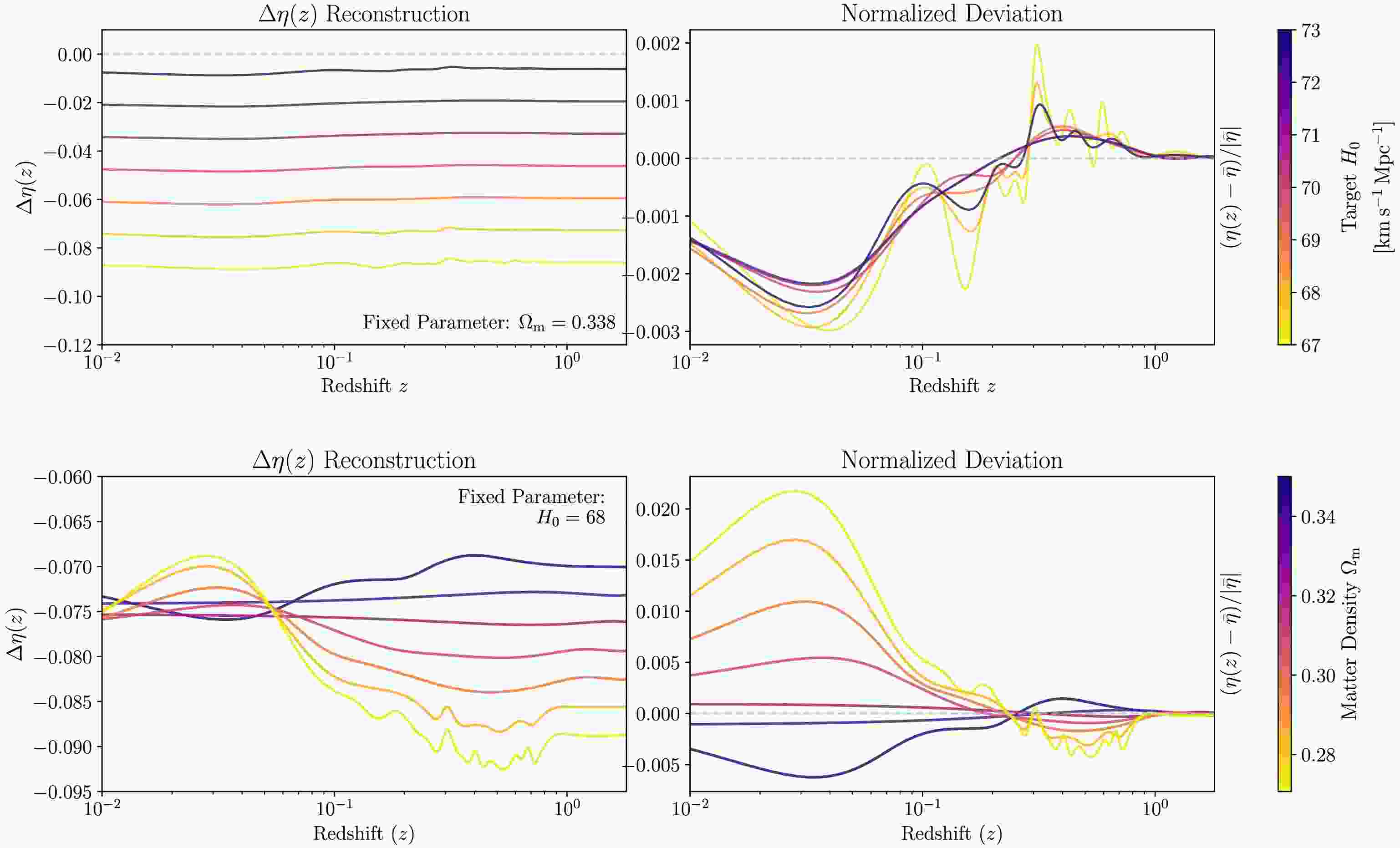
For Fig. 1, we use smooth, localized Gaussian functions.
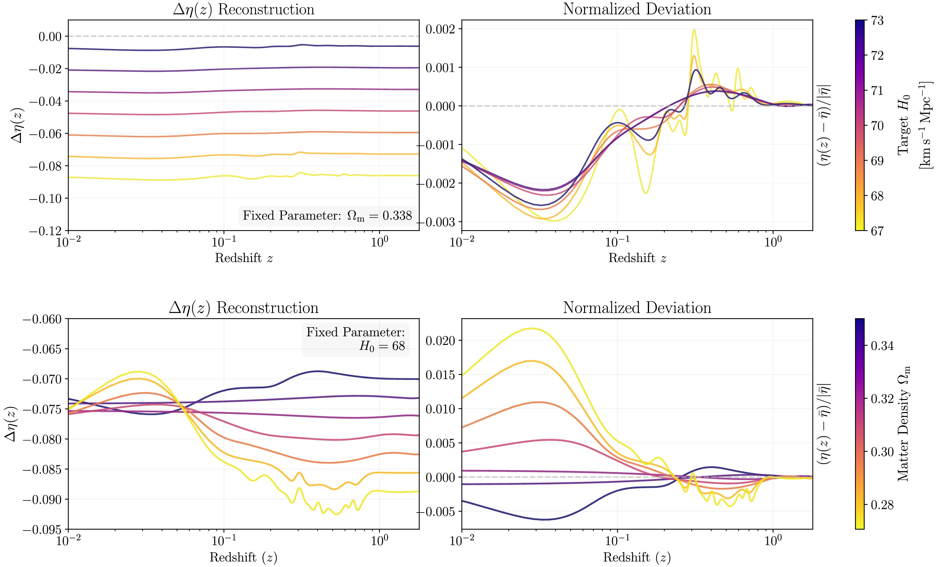
Figure 1. (color online) Solutions for the
$ \Delta\eta(z)=\eta(z)-1 $ profiles for specified target values of$ H_0 $ and$ \Omega_m $ . The upper row shows results for fixed$ \Omega_m=0.338 $ with different target$ H_0 $ values; the lower row shows results for fixed$ H_0=68 $ km s−1 Mpc−1 with different target$ \Omega_m $ values. All$ H_0 $ values in the figure are given in km s−1 Mpc−1. The left panels show$ \Delta\eta $ , and the right panels show$ (\eta-\bar\eta)/|\bar\eta| $ .$ \phi_i^{\rm{G}}(z)=\exp \left[-\frac{(z-z_i)^2}{2\sigma^2}\right], $
(3) with equally spaced centres on the interval
$ 0\leq z\leq2 $ . The width parameter in equation (3) follows the numerical convention of Ref. [24]: the full width at half maximum is equal to the centre spacing:$ \Delta z=\frac{2}{N-1},\qquad \sigma=\frac{\Delta z}{2\sqrt{2\ln2}}. $
(4) For
$ N=80 $ , equation (4) yields$ \Delta z\simeq0.0253 $ and$ \sigma\simeq0.01075 $ . Equal spacing and equal widths provide uniform numerical resolution. An adaptive basis would require a prescription specifying how that resolution varies with redshift; we use the uniform choice to explore broad trends without introducing such a prescription.We choose
$ N=80 $ to explore these trends with a flexible function before selecting a compact parameterization. The spacing is finer than the broad features relevant to this purpose. The comparison with$ N=60 $ and$ 100 $ in Section 2.3 evaluates this choice at a common display scale while keeping the width-to-spacing relation fixed. The number of centres controls the numerical flexibility of the representation; it should not be interpreted as the number of physical modes constrained by the data. Figure 2 also includes an illustrative calculation with a top-hat basis: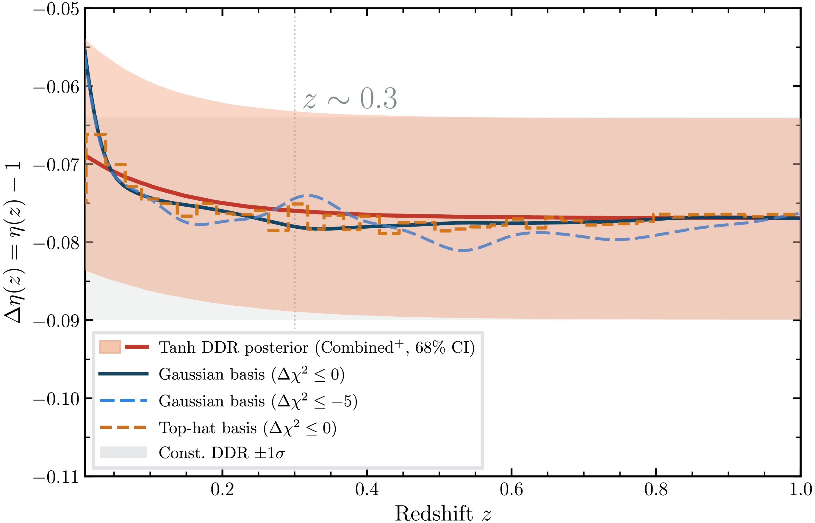
Figure 2. (color online) Comparison of illustrative Fisher-bias
$ \Delta\eta(z) $ profiles with the posterior band inferred from MCMC for the three-parameter tanh model. The red shaded region shows the 68 per cent credible interval for$ \Delta\eta(z) \equiv \eta(z) - 1 $ obtained from the Combined+ dataset ($ A = -0.078 \pm 0.013 $ ,$ z_t = -0.289^{+0.036}_{-0.11} $ ,$ \Delta = 0.199 \pm 0.10 $ ); the solid red line indicates the posterior median. The dark blue solid and light blue dotted curves show the Gaussian-basis Fisher-bias reconstructions targeting the Planck+BAO ΛCDM best-fit parameters ($ \omega_c = 0.1202 $ ,$ H_0 = 68.4 $ km s−1 Mpc−1) under the constraints$ \Delta\chi^2_{\rm{BF}} \leq 0 $ and$ \Delta\chi^2_{\rm{BF}} \leq -5 $ , respectively; the orange dashed curve shows the binned-basis check under$ \Delta\chi^2_{\rm{BF}} \leq 0 $ . The legend's$ \Delta\chi^2 $ refers to the locally profiled quadratic Fisher-bias statistic in equation (10), not to a full nonlinear likelihood refit. The constrained profiles lie within the 68 per cent MCMC band over$ z\in[0,1] $ ; this comparison motivates the broad transition but does not constitute an independent measurement of its shape.$ \phi_i^{\rm{TH}}(z)= \begin{cases}1,&|z-z_i|<\Delta z/2,\\0,&\text{otherwise}. \end{cases} $
(5) -
The Fisher-bias formalism estimates shifts in fitted cosmological parameters induced by small changes in the predicted observables [24, 28, 29]. Following the response calculation of Ref. [24], let
$ {\boldsymbol{X}}({\bf{\Omega}},{\boldsymbol{c}}) $ denote the supernova prediction vector,$ {\boldsymbol{X}}_{\rm{obs}} $ the observations, and C their covariance matrix. The Gaussian fit statistic is$ \chi^2({\bf{\Omega}},{\boldsymbol{c}})= [{\boldsymbol{X}}({\bf{\Omega}},{\boldsymbol{c}})-{\boldsymbol{X}}_{\rm{obs}}]^T {\boldsymbol{C}}^{-1} [{\boldsymbol{X}}({\bf{\Omega}},{\boldsymbol{c}})-{\boldsymbol{X}}_{\rm{obs}}]. $
(6) For the SN fit statistic in equation (6), the varied parameters are
$ {\bf{\Omega}}=(\omega_c,h_0) $ , while the baryon density and magnitude calibration are held fixed. Here,$ h_0\equiv H_0/(100\,\mathrm{km\,s^{-1}\,Mpc^{-1}}) $ .Linearizing the predictions about the undeformed cosmology yields
$ \delta{\boldsymbol{X}}\simeq{\boldsymbol{J}}\,\delta{\bf{\Omega}} +{\boldsymbol{B}}{\boldsymbol{c}}, \qquad J_{a\alpha}=\frac{\partial X_a}{\partial\Omega_\alpha},\quad B_{ai}=\frac{\partial X_a}{\partial c_i}. $
(7) In equation (7), a labels the observations, α the cosmological parameters, and i the basis functions; the derivatives are evaluated at zero deformation. For magnitude observables, the distance rescaling gives
$ \delta\mu(z)=5\log_{10}[1+\Delta\eta(z)] $ , and therefore$ B_{ai}=5\phi_i(z_a)/\ln10 $ .Writing
$ {\boldsymbol{M}}={\boldsymbol{C}}^{-1} $ and$ {\boldsymbol{F}}={\boldsymbol{J}}^T{\boldsymbol{M}}{\boldsymbol{J}} $ , the Fisher matrix describes the curvature of the quadratic fitting statistic in parameter space. Minimizing this statistic with respect to the cosmological parameters and subtracting the zero-deformation stationarity condition gives$ {\boldsymbol{F}}\,\Delta{\bf{\Omega}}_{\rm{BF}} +{\boldsymbol{J}}^T{\boldsymbol{M}}{\boldsymbol{B}}{\boldsymbol{c}}=0. $
(8) Solving equation (8) yields the induced parameter shift,
$ \Delta{\bf{\Omega}}_{\rm{BF}}[\Delta\eta] \simeq-{\boldsymbol{F}}^{-1}{\boldsymbol{J}}^T{\boldsymbol{M}} {\boldsymbol{B}}{\boldsymbol{c}}. $
(9) Substituting the fitted response into the quadratic statistic yields the change in its minimum. Define the undeformed residual
$ {\boldsymbol{r}}={\boldsymbol{X}}_{\rm{fid}}-{\boldsymbol{X}}_{\rm{obs}} $ and$ \widetilde{{\boldsymbol{M}}}={\boldsymbol{M}}-{\boldsymbol{M}}{\boldsymbol{J}} {\boldsymbol{F}}^{-1}{\boldsymbol{J}}^T{\boldsymbol{M}} $ , which accounts for the adjustment of the cosmological parameters. Then$ \Delta\chi^2_{\rm{BF}}[\Delta\eta]\simeq 2{\boldsymbol{r}}^T\widetilde{{\boldsymbol{M}}}{\boldsymbol{B}}{\boldsymbol{c}} +{\boldsymbol{c}}^T{\boldsymbol{B}}^T\widetilde{{\boldsymbol{M}}} {\boldsymbol{B}}{\boldsymbol{c}}. $
(10) These expressions retain the linear parameter response and the change in the fit statistic through quadratic order in the observable perturbation, as in Ref. [24]. Within this approximation, equation (9) maps a trial distance deformation onto the corresponding shift in the best-fit cosmological parameters, whereas equation (10) quantifies whether this deformation improves or degrades the fit after those parameters are adjusted.
For a chosen cosmological target, we minimize the redshift variation while maintaining or improving the fit. Within the Fisher-bias approximation, the constrained problem is
$ \begin{array}{l} \underset{{\boldsymbol{c}}}{\text{minimize}}\quad \int_0^2 dz\,[\eta(z)-\bar\eta]^2,\\ \text{subject to}\quad \begin{cases} {\bf{\Omega}}_{\rm{BF}}[\Delta\eta(z)]={\bf{\Omega}}_{\rm{target}},\\ \Delta\chi^2_{\rm{BF}}[\Delta\eta(z)]\leq0. \end{cases} \end{array} $
(11) where
$ \bar\eta=\dfrac12\int_0^2\eta(z)\,dz $ . The penalty quantifies variation about the mean, without imposing a separate penalty on the mean calibration offset. Both constraints in equation (11) are evaluated using the full distance deformation, including its mean component. The mean is therefore determined jointly with the shape in the constrained problem. The relation between the two possible penalties is$ \eta-\bar\eta=\Delta\eta-\overline{\Delta\eta},\qquad \int_0^2(\Delta\eta)^2dz= \int_0^2(\eta-\bar\eta)^2dz+2\overline{\Delta\eta}^{\,2}, $
(12) where
$ \overline{\Delta\eta}\equiv\frac12\int_0^2\Delta\eta(z)\,dz =\bar\eta-1. $
(13) Equation (12), with the mean defined in equation (13), shows that minimizing
$ \int(\Delta\eta)^2dz $ would also penalize the mean offset. Our choice seeks the minimum redshift variation associated with the allowed recalibration and can therefore yield a different profile.Substituting equation (2) yields a quadratic objective
$ {\boldsymbol{c}}^T{\boldsymbol{Q}}{\boldsymbol{c}} $ , with$ Q_{ij}=\int_0^2[\phi_i(z)-\bar\phi_i][\phi_j(z)-\bar\phi_j]dz $ and$ \bar\phi_i=\dfrac12\int_0^2\phi_i(z)dz $ . Together with the linear target condition and the quadratic fit-quality condition, this defines a deterministic constrained optimization problem. -
For the resolution check, we use the fourteen specified
$ (H_0,\Omega_m) $ parameter pairs shown in Fig. 1: seven$ H_0 $ values from 67 to 73 km s−1 Mpc−1 at fixed$ \Omega_m=0.338 $ , and seven$ \Omega_m $ values spanning approximately 0.270–0.350 at fixed$ H_0=68 $ km s−1 Mpc−1. For each parameter pair, the profiles obtained with$ N=60 $ ,$ 80 $ , and$ 100 $ show similar broad trends after Gaussian smoothing with$ \sigma_s=0.05 $ , as defined below. This comparison supports the adequacy of the resolution for the compact description. The smoothed comparison profiles summarize the broad trend of the underlying optimized functions; the constraints are evaluated before smoothing.For a representative target with lower matter density at fixed
$ H_0=68\,\mathrm{km\,s^{-1}\,Mpc^{-1}} $ and$ \Omega_m\simeq0.297 $ , we also use$ N=80 $ top-hat functions from equation (5), with the same target, variation penalty, and fit-quality condition. To compare the broad trend on a common redshift scale, we evaluate each optimized profile on a uniform grid and convolve it with a normalized Gaussian of width$ \sigma_s=0.05 $ , using reflection at$ z=0 $ and 2. For the top-hat basis, this operation is applied to the piecewise-constant function after optimization. The broad decrease with redshift is retained with either basis, supporting the robustness of this trend to the tested basis choice.We retain the overall normalization and a broad transition as the information relevant to a simple physical test: whether redshift variation is supported beyond an overall distance recalibration. Local excursions are not assigned physical significance by this construction. The three tanh parameters are fitted directly in the full likelihood, with the model specified in Section 3.3. The number of basis functions and the smoothed profiles are not inputs to that likelihood.
-
The SN target scans use the calibrated Pantheon+ distance sample, with the magnitude calibration and BBN-motivated baryon density held fixed. We specify target values of
$ H_0 $ and$ \Omega_m $ and reconstruct the distance deformation using the Fisher-bias responses and constraints described in Section 2.2. CMB and BAO information guides the choice of target values; their likelihoods are included in the full statistical analysis in Section 4. -
The upper row of Fig. 1 fixes
$ \Omega_m=0.338 $ while varying the target$ H_0 $ ;$ \bar\eta $ denotes the mean over the reconstruction range. The left panels show the deviation$ \Delta\eta=\eta-1 $ . For target values$ H_0 \gtrsim 70\; \mathrm{km\,s^{-1}\,Mpc^{-1}} $ ,$ \eta(z) $ remains nearly constant, with fractional deviations satisfying$ (\eta(z)-\bar{\eta})/\bar{\eta}\lesssim0.02 $ . As the target value$ H_0\sim73\; \mathrm{km\,s^{-1}\,Mpc^{-1}} $ approaches the SN-calibrated reference scale, the overall deformation becomes small. For a target value$ H_0\simeq68\; \mathrm{km\,s^{-1}\,Mpc^{-1}} $ , the average normalization is instead$ \bar\eta\simeq0.93 $ , close to the effective calibration offset reported by Teixeira et al. [14].The lower row fixes
$ H_0 = 68\; \mathrm{km\,s^{-1}\,Mpc^{-1}} $ while varying the target$ \Omega_m $ . In this configuration, both the amplitude and the shape of$ \eta(z) $ depend sensitively on$ \Omega_m $ . For$ z \gtrsim 0.1 $ ,$ \eta(z) $ increases when$ \Omega_m $ is raised above the Pantheon+SH0ES best-fit value and decreases when$ \Omega_m $ is lowered. When$ \Omega_m $ is reduced to$ \sim 0.28 $ , the fractional deviation$ (\eta(z)-\bar{\eta})/|\bar{\eta}| $ becomes of order one percent, indicating that reconciling Pantheon+SH0ES with such a low matter density is accompanied by a broad redshift trend in the conditional profiles.A key implication concerns the alternative strategy of reshaping the background expansion rate
$ E(z) $ rather than$ \eta(z) $ . A suppressed expansion rate ($ \delta E<0 $ at$ z\lesssim0.5 $ )—the low-redshift deformation invoked to raise the inferred$ H_0 $ —increases the luminosity distance.$ \frac{\delta D_L}{D_L} \propto -\int_0^z \frac{\delta E(z')}{E^2(z')}\,dz' \gt 0\,. $
(14) Because equation (14) shows that Pantheon constrains the shape of
$ D_L(z) $ whereas SH0ES fixes its normalization, this excess must be compensated by a higher SN-inferred$ \Omega_m $ . The same low-redshift phantom transition ($ w<-1 $ ) that raises$ H_0 $ therefore pushes the SN-inferred$ \Omega_m $ upward, whereas lowering it requires the opposite, quintessence-like deformation ($ w>-1 $ ). To linear order in the Fisher-bias response, the minimal-amplitude$ w(z) $ deformations that achieve these two goals point in opposite directions, so a single such deformation cannot meet both [24, 25]. This shape-derived$ \Omega_m $ should be distinguished from the global matter density of a CMB-anchored fit,$ \Omega_m=(\omega_b+\omega_c+\omega_\nu)/h_0^2 $ , for which tightly constrained physical densities tie$ \Omega_m $ to$ H_0 $ .In contrast, a redshift-dependent
$ \eta(z) $ can directly shift the SN-inferred$ \Omega_m $ (Fig. 1) without simultaneously driving it upward through the expansion history. The reconstructed profiles therefore show that the required deformation depends jointly on the target$ H_0 $ and$ \Omega_m $ : the late- versus early-Universe calibration problem is intrinsically multidimensional rather than reducible to a shift in$ H_0 $ alone. -
The reconstructions above demonstrate that
$ \eta(z) $ alone can shift the matter density inferred from the SNe-only (Pantheon+SH0ES) likelihood, but this deformation does not propagate to the BAO+CMB sector. In the full combined fit, by contrast,$ \Omega_m $ is essentially fixed by CMB+BAO and is nearly identical for the constant and tanh DDR models; see Section 5.2. Because$ \omega_c \equiv \Omega_c h_0^2 $ and$ \omega_b \equiv \Omega_b h_0^2 $ are tightly constrained by the CMB and BBN likelihoods, increasing$ H_0 $ necessarily lowers$ \Omega_m = \Omega_c + \Omega_b + \Omega_\nu $ . A natural question is therefore whether simultaneous modifications to$ \eta(z) $ and the expansion history$ H(z) $ can reconcile the SNe and BAO/CMB constraints. This exercise also exposes the degeneracy between geometric (DDR) and dynamical (dark energy) modifications at the background level.Our strategy is as follows. Using BAO measurements calibrated with the CMB-inferred sound horizon
$ r_s $ , we fix$ \omega_c = 0.1202 $ and impose a target$ H_0 $ . We then obtain an optimal$ w(z) $ profile using the Fisher-bias method. This model serves as the new baseline, with the Pantheon+SH0ES best-fit values within this model used as the reference parameters. We subsequently apply the Fisher-bias method again, fixing$ \omega_c = 0.1202 $ and the same$ H_0 $ target, to reconstruct the corresponding$ \eta(z) $ profile.Figure 3 shows the results for different
$ H_0 $ targets. The upper panel presents the reconstructed$ w(z) $ , and the lower panel presents the corresponding$ \Delta\eta(z)=\eta(z)-1 $ . The equation of state crosses the phantom divide around$ z \sim 0.3 $ , evolving from$ w \lt -1 $ at$ z \lt 0.3 $ to$ w \gt -1 $ thereafter. In response,$ \eta(z) $ develops a pronounced dip, with higher$ H_0 $ targets producing deeper dips centred near$ z \sim 0.5 $ . The profile mildly rebounds near$ z \sim 1 $ and becomes approximately constant for$ z \gt 1 $ . This behaviour is consistent with the independently reconstructed$ \eta(z) $ -only deformation, confirming that reducing the Pantheon-inferred$ \Omega_m $ requires a declining$ \eta(z) $ profile.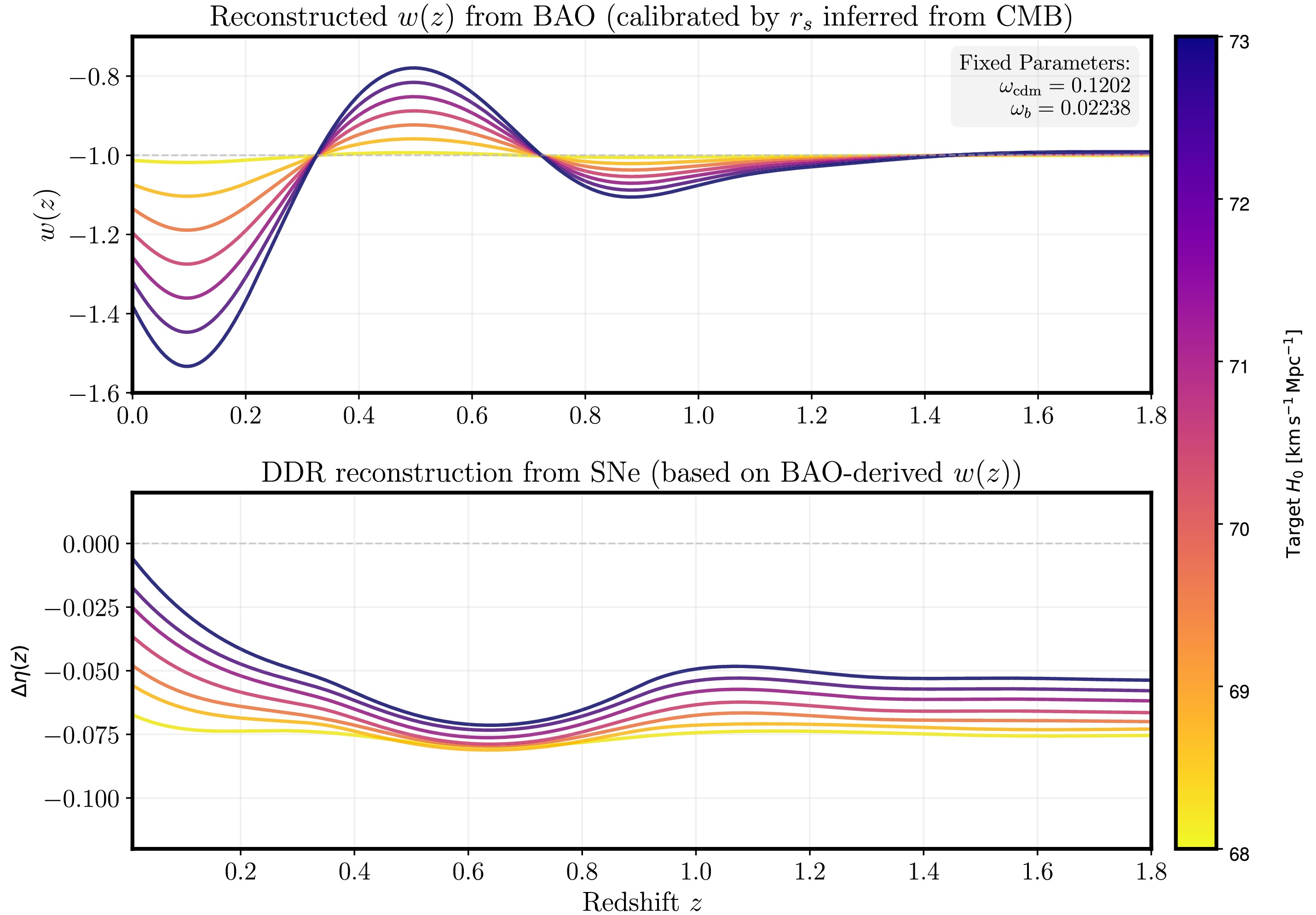
Figure 3. (color online) Conditional
$ w(z) $ and DDR-deformation profiles. The upper panel shows$ w(z) $ reconstructed from BAO and the CMB-calibrated sound horizon, with$ \omega_c=0.1202 $ and the indicated target$ H_0 $ . The lower panel shows$ \Delta\eta(z)=\eta(z)-1 $ from the corresponding Fisher construction in the SN sector at the same$ \omega_c $ and$ H_0 $ . The colour bar indicates$ H_0 $ in km s−1 Mpc−1. Parameters not varied here are fixed at their Planck ΛCDM best-fit values.Physically, the dip arises from the response of the luminosity distance to a reduced matter density. In a flat cosmology with fixed
$ H_0 $ , decreasing$ \Omega_m $ lowers the background expansion rate in the matter-dominated regime:$ E(z) = \frac{H(z)}{H_0} = \sqrt{\Omega_m(1+z)^3 + \Omega_\Lambda}\,, \qquad \partial_{\Omega_m}E(z)>0\,. $
(15) Equation (15) implies that the luminosity distance increases,
$ D_L(z) \propto \int_0^z \frac{dz'}{E(z')}\,, \qquad \partial_{\Omega_m}D_L(z)<0 \quad \text{for } z\sim0.3\text{–}1\,. $
(16) Since Pantheon constrains the distances, the response in equation (16) must be compensated by a suppressing
$ \eta(z) $ deformation over the same redshift range. The conditional dip illustrates the compensating deformation associated with the$ D_L $ response to a reduced$ \Omega_m $ , while preserving the low-z normalization (SH0ES calibration) and high-z asymptotic behaviour.The reconstructed
$ w(z) $ and$ \eta(z) $ profiles produce nearly identical predictions for the observed luminosity distances in this construction. A phantom-like transition in$ w(z) $ at low redshift suppresses$ E(z) $ and increases$ D_L $ ; a dip in$ \eta(z) $ compensates for that response. Thus, the specific effective SN-sector$ \eta(z) $ and$ w(z) $ models considered here are strongly degenerate at the background level. Direct measurements of$ H(z) $ , such as cosmic chronometers or radial BAO$ D_H(z)=c/H(z) $ , probe the expansion component of this particular degeneracy. -
We distinguish two conditional constructions. For the SN-sector-only profiles of Section 3.1, the retained compact information consists of an overall normalization and a broad redshift trend. When
$ \eta(z) $ and$ w(z) $ are varied jointly (Section 3.2),$ \eta(z) $ develops a dip that compensates for the imposed change in$ E(z) $ . Because the MCMC model below varies only the SN luminosity distance, we use the former construction to motivate a single broad transition. The smooth-kernel and binned-basis checks in Fig. 2 agree to the accuracy relevant for this limited purpose; they are not independent data-driven measurements of$ \eta(z) $ .The physical question is whether the data support a broad redshift variation beyond the overall distance recalibration. We therefore use a tanh function, which connects two asymptotic normalizations through a single transition and includes an approximately constant limit over the observed range. This compact form captures the broad behavior of interest without fitting individual excursions in the numerical profiles. We therefore adopt
$ \eta(z) = 1 + A\,\tanh \left(\frac{z - z_t}{\Delta}\right), $
(17) where A sets the asymptotic deviation amplitude,
$ z_t $ locates the transition, and δ sets its width. All three hyperbolic-tangent parameters are sampled jointly with the cosmological parameters in the full likelihood; their values are determined by the data within the adopted priors. The numerical reconstructions motivate this functional form, but they neither fix the parameter values nor enter the likelihood. As discussed in Section 5.2, the fitted transition centre is slightly negative, so the model is close to a constant offset with a mild residual gradient across the observed range. This form has three useful limiting behaviours:1.
$ A = 0 $ : the standard DDR, recovering ΛCDM;2.
$ -z_t/\Delta\gg1 $ : an approximately constant offset over the observed range,$ \eta(z)\simeq1+A $ , which is degenerate with a shift in$ M_B $ ;3. finite A,
$ z_t $ , and δ: a redshift-dependent term in the adopted effective model.The first two limits are nested within the full parameterization, enabling direct model comparisons using
$ \Delta\chi^2 $ , the Akaike information criterion (AIC), the deviance information criterion (DIC), and the Bayesian evidence (Section 5.2). -
The DDR modification is implemented in the Python wrapper of the Einstein–Boltzmann code CLASS [31, 32]. The rescaling
$ D_L^{\rm{obs}}(z)=\eta(z)D_L^{\rm{GR}}(z) $ is applied only to the luminosity distance used in the supernova likelihood. BAO distances, the CMB likelihood, cosmic-chronometer predictions, the background expansion, and the perturbation equations remain unchanged. The fitted$ \eta(z) $ should therefore be interpreted solely as the effective SN-sector response defined in Section 2.We consider three nested models:
1. ΛCDM: the standard model with
$ \eta(z) = 1 $ ;2. Constant DDR: a redshift-independent offset,
$ \eta(z) = \eta_0 $ . In the absence of an external absolute-magnitude prior, this offset is exactly degenerate with a shift in the supernova absolute magnitude$ M_B $ ; this degeneracy is broken once the SH0ES calibration is imposed. In Table 1, the Combined+ entry corresponds to a one-parameter chain with free$ \eta_0 $ , yielding$ \eta_0 = 0.925 \pm 0.013 $ , whereas the Combined- entry fixes the representative value$ \eta_0 = 0.925 $ , consistent with Teixeira et al. [14];Model Dataset A $ z_t $ δ $ H_0 $ [km s−1 Mpc−1]$ \Omega_m $ $ S_8 $ $ \chi^2 $ Tanh DDR BAO+SNe $ -0.069\pm0.015 $ $ -0.272\pm0.090 $ $ 0.204\pm0.103 $ $ 69.07\pm0.49 $ $ 0.301\pm0.008 $ $ 0.814\pm0.032 $ $ 1297.7 $ Combined- $ -0.052\pm0.050 $ $ -0.206\pm0.132 $ $ 0.202\pm0.104 $ $ 68.42\pm0.31 $ $ 0.301\pm0.004 $ $ 0.807\pm0.010 $ $ 2443.8 $ Combined+ $ -0.078\pm0.013 $ $ -0.289^{+0.036}_{-0.11} $ $ 0.199 \pm 0.10 $ $ 68.44\pm0.30 $ $ 0.301\pm0.004 $ $ 0.806\pm0.010 $ $ 2321.2 $ Constant DDR Combined- $ -0.075 $ (fixed)— — $ 68.32\pm0.30 $ $ 0.302\pm0.004 $ $ 0.809\pm0.009 $ $ 2447.7 $ Combined+ $ -0.075\pm0.013 $ — — $ 68.38\pm0.28 $ $ 0.301\pm0.004 $ $ 0.808\pm0.010 $ $ 2324.8 $ ΛCDM Combined- — — — $ 68.76^{+0.17}_{-0.20} $ $ 0.297\pm0.003 $ $ 0.803^{+0.008}_{-0.009} $ $ 2448.8 $ Combined+ — — — $ 68.82\pm0.26 $ $ 0.296\pm0.003 $ $ 0.800^{+0.009}_{-0.008} $ $ 2356.3 $ Table 1. Cosmological parameter constraints for the tanh DDR, constant DDR, and ΛCDM models for different dataset combinations. All values are reported as means
$ \pm 1\sigma $ credible intervals; asymmetric errors are shown where the posterior is non-Gaussian. “BAO+SNe” denotes BAO + Pantheon+SH0ES + BBN. “Combined-” includes Planck and CC but excludes the SH0ES calibration; “Combined+” further includes SH0ES. For the Combined+ dataset, the constant-DDR row corresponds to a free one-parameter chain, yielding$ \eta_0 = 1+A = 0.925 \pm 0.013 $ (a$ 5.7\sigma $ deviation from unity), consistent with Teixeira et al. [14]; the Combined- constant-DDR entry fixes$ \eta_0 = 0.925 $ . Dashes indicate parameters that are not present in the corresponding model.3. Tanh DDR: the three-parameter model given by equation (17), which reduces to (i) when
$ A=0 $ and approaches (ii) when$ -z_t/\Delta\gg1 $ over the observed redshift range.The nested structure enables direct model comparison using
$ \Delta\chi^2 $ , the AIC, the DIC, and the Bayesian evidence. For the tanh model, we adopt flat priors$ A \in [-0.15,\,0.10] $ ,$ z_t \in [-0.40,\,0.20] $ , and$ \Delta \in [0.02,\,0.40] $ for all dataset combinations. The marginal posteriors lie within these ranges, although the$ z_t $ posterior approaches the lower bound while its peak remains well inside it (see below). The A prior is deliberately asymmetric about zero: the calibration mismatch fixes the sign of the offset—a suppressed supernova luminosity distance,$ \eta<1 $ (i.e.$ A<0 $ )—so the prior extends further in the negative direction while retaining a positive margin as a null check. Negative$ z_t $ values are permitted because the transition centre may physically lie below the observed redshift range. In this case,$ \eta(z) $ varies only mildly over$ z\ge0 $ and approaches the constant-offset limit while remaining well defined for all$ z\ge0 $ . The combined-fit$ z_t $ posterior extends toward this lower bound, with its$ 1\sigma $ interval reaching$ z_t \simeq -0.40 $ , i.e. toward the constant-offset direction$ z_t \to -\infty $ . However, this truncation does not drive our conclusions, because the approach to the constant limit is probed independently by the prior reweighting in$ r = -z_t/\Delta $ (Section 5.2) and by the free one-parameter constant-DDR chain, neither of which is sensitive to the$ z_t $ boundary. -
We combine multiple cosmological probes spanning different redshifts and physical scales:
DESI BAO (DR2).—The Dark Energy Spectroscopic Instrument Data Release 2 [33] provides BAO measurements from 14 million extragalactic objects in nine redshift bins over
$ 0.295 \leq z \leq 2.330 $ . These are reported as$ (D_M/r_d,\,D_H/r_d) $ with the full non-diagonal covariance matrix.Pantheon+ and SH0ES.—The Pantheon+ compilation [34, 35] provides distance moduli from 1701 light curves of 1550 spectroscopically confirmed SNe Ia over
$ 0.001 \lt z \lt 2.26 $ . We analyse this dataset both with and without the SH0ES Cepheid calibration [5], implemented through the full Pantheon+SH0ES likelihood following Poulin et al. [12].Cosmic chronometers.—We use 32 direct
$ H(z) $ measurements from differential galaxy aging [36−42], as compiled by Wu [43], spanning$ 0.07 \lt z \lt 1.97 $ . These measurements are included specifically because they constrain$ H(z) $ directly, independently of integrated distance measures. They therefore provide a means of constraining the$ \eta(z) $ –$ H(z) $ degeneracy identified in Section 3.2; we quantify their current, limited constraining impact in Section 5.3.Planck CMB.—For the Fisher-bias analysis, we use the CMB distance priors from the Planck 2018 release [44], comprising the shift parameter
$ {\cal{R}} $ , the acoustic scale$ \ell_A $ , and$ \Omega_b h_0^2 $ . The MCMC analysis uses the 2018 Commander low-ℓ TT, SimAll low-ℓ EE, and Plik-lite high-ℓ TT+TE+EE likelihoods [45, 46]; the four-point CMB-lensing likelihood is not included.We denote the combination CC + BAO + SNe + Planck as “Combined-” (excluding the SH0ES calibration) and the same combination with SH0ES included as “Combined+”.
-
MCMC analyses were performed with MONTEPYTHON 3.6
1 [47] using the Metropolis–Hastings algorithm and were analyzed with GETDIST [48]. We sampled the six standard flat-ΛCDM parameters, the Planck calibration nuisance parameter, the SN absolute magnitude, and the DDR parameters included in each model. We assumed one massive neutrino with$ \sum m_\nu=0.06 $ eV and$ N_{\rm{ur}}=2.0328 $ , and used the standard BBN-consistent helium prescription. The BBN likelihood used PArthENoPE predictions with the deuterium abundance$ 10^5({\rm{D/H}})=2.527\pm0.030 $ and the helium abundance$ Y_p=0.2449\pm0.0040 $ . We required$ R-1<0.05 $ [49]. For the main Combined+ tanh result, we used six chains (56,765 total Metropolis steps; 21,447 accepted). The independent MULTINEST evidence calculation used 400 live points, importance nested sampling, and an evidence tolerance of 0.5.AI-tool disclosure. OpenAI Codex was used for language checking and editing.
-
Figure 4 summarizes the posterior comparisons across dataset combinations and among ΛCDM, constant DDR, and tanh DDR. We perform Markov Chain Monte Carlo (MCMC) analyses using the tanh parameterization of equation (17), in which the DDR parameters (A,
$ z_t $ , δ) are sampled freely alongside the standard cosmological parameters. The datasets, priors, and sampling methodology are described in Section 4.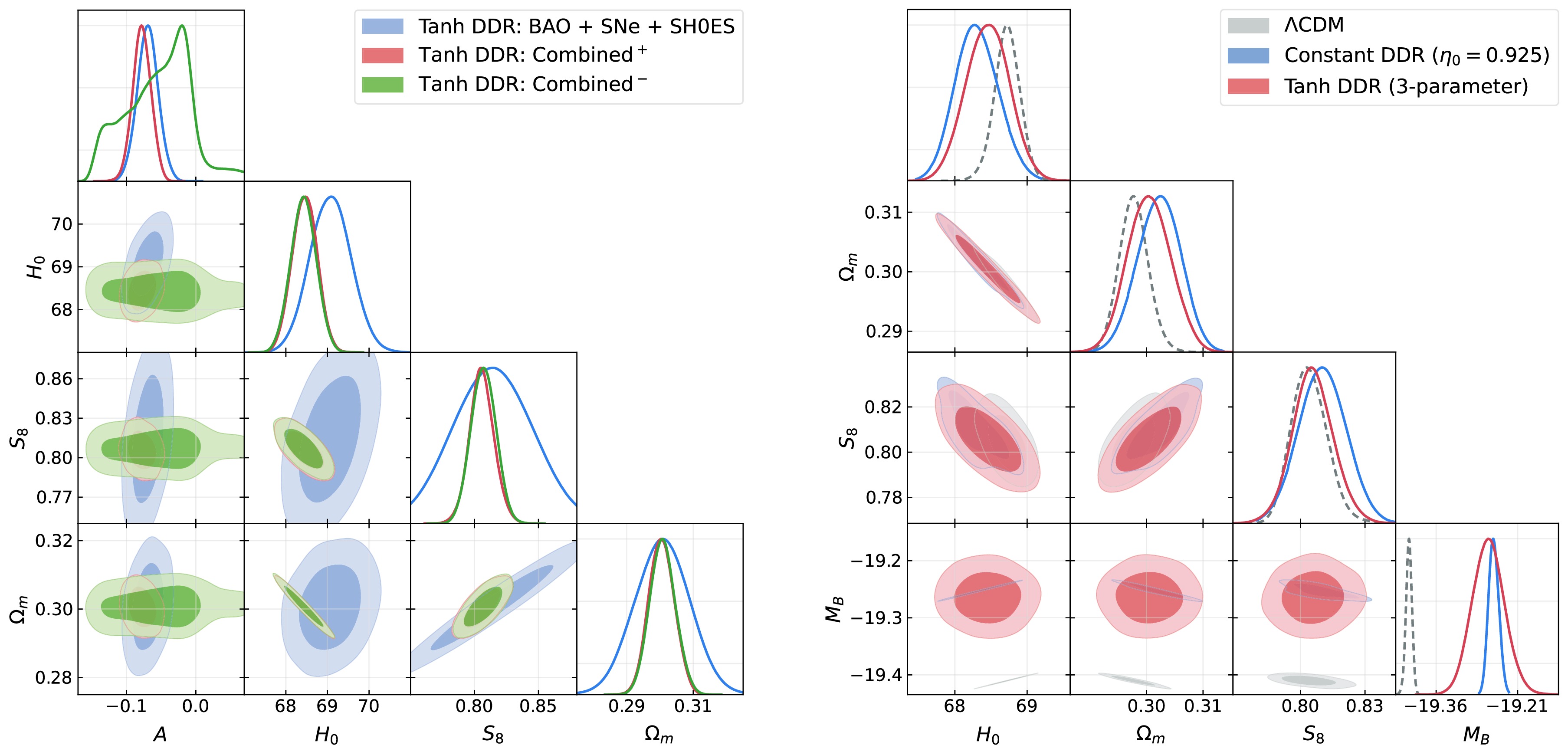
Figure 4. (color online) Posterior distributions for cosmological parameters. Left: Constraints from the three-parameter tanh DDR model for three dataset combinations: BAO+Pantheon+SH0ES (blue), Combined+ (red), and Combined- (green). The contours are mutually consistent. The DDR amplitude A is tightly constrained when the SH0ES calibration is included (blue, red), but remains broad for Combined- (green), where A is nearly degenerate with the supernova absolute magnitude
$ M_B $ . Nevertheless, the cosmological parameters ($ H_0 $ and$ \Omega_m $ ) agree across all three combinations, indicating that they are not driven by the DDR amplitude or by any single calibration choice. Right: Comparison of ΛCDM (grey dashed), constant DDR (blue), and tanh DDR (red) for the Combined+ dataset. The tanh DDR model shifts$ M_B $ and yields an$ H_0 $ value consistent with the Planck baseline, while$ \Omega_m $ remains close to its ΛCDM value. The constant DDR model recovers$ H_0 $ and$ \Omega_m $ values similar to those of the tanh model and likewise shifts$ M_B $ away from its ΛCDM value, reflecting the degeneracy between a constant DDR offset and a recalibration of the supernova absolute magnitude. All contours show 68 and 95 per cent credible regions. -
Table 1 summarizes the constraints on the DDR and cosmological parameters. For the Combined+ dataset, we find
$ \begin{array}{l} A = -0.078 \pm 0.013\,, \\ z_t = -0.289^{+0.036}_{-0.11}\,, \\ \Delta = 0.199 \pm 0.10\,, \end{array} $
(18) Equation (18) presents the fitted DDR parameters; the inferred cosmological parameters are
$ \begin{array}{l} H_0 = 68.44 \pm 0.30\; \mathrm{km\,s^{-1}\,Mpc^{-1}}\,,\\ \Omega_m = 0.301 \pm 0.004\,. \end{array} $
(19) The values in equation (19) are fully consistent with the Planck ΛCDM baseline and do not require any modification to the expansion history.
For the Combined- dataset (no SH0ES), the DDR amplitude is only weakly constrained,
$ A = -0.052 \pm 0.050 $ , with$ z_t = -0.206 \pm 0.132 $ and$ \Delta = 0.202 \pm 0.104 $ . The cosmological parameters nevertheless remain stable, with$ H_0 = 68.42 \pm 0.31 $ km s−1 Mpc−1 and$ \Omega_m = 0.301 \pm 0.004 $ .The broad A posterior in Combined- is a direct consequence of the nearly exact degeneracy between the DDR amplitude and the supernova absolute magnitude
$ M_B $ after the SH0ES calibration is removed. In this chain, A and$ M_B $ are anti-correlated with$ \rho = -0.99 $ , so without the Cepheid anchor the data constrain essentially only the combination of A and$ M_B $ , rather than A itself. The amplitude is therefore well determined only when SH0ES is included (Combined+:$ A = -0.078 \pm 0.013 $ ; BAO+SNe:$ A = -0.069 \pm 0.015 $ ). Both analyses retain the anchor, so the apparent “shift” in A across combinations reflects this degeneracy rather than a physical change in the DDR amplitude. The$ H_0 $ and$ \Omega_m $ posteriors are consistent across all three combinations, confirming that these cosmological parameters are constrained by the CMB and BAO data rather than by the DDR deformation itself.As an additional cross-check, the BAO+SNe analysis (without Planck or CC) yields
$ A = -0.069 \pm 0.015 $ ,$ z_t = -0.272 \pm 0.090 $ , and$ \Delta = 0.204 \pm 0.103 $ , with$ H_0 = 69.07 \pm 0.49 $ km s−1 Mpc−1 and$ \Omega_m = 0.301 \pm 0.008 $ . The fitted effective and cosmological parameters are consistent with the Combined+ result within$ 1\sigma $ . This does not by itself establish a physical DDR signal, because the dominant amplitude is the calibration-degenerate constant component quantified below. -
A central question is whether the data favor redshift-dependent structure beyond a constant effective offset in the SN sector. For Combined+, the essential decomposition is
$ \Delta\chi^2_{ {\rm{tanh}}/\Lambda {\rm{CDM}}}=-35.1,\qquad \Delta\chi^2_{ {\rm{const}}/\Lambda {\rm{CDM}}}=-31.5, $
(20) Thus, equation (20) implies an incremental gain attributable to redshift structure of
$ \Delta\chi^2_{\rm{tanh/const}}=-3.6 $ for two additional parameters. The corresponding minimum values are$ \chi^2=2356.3 $ ,$ 2324.8 $ , and$ 2321.2 $ for ΛCDM, constant DDR, and tanh DDR, respectively. In the tanh model, the constant limit is approached when$ r\equiv-z_t/\Delta\gg1 $ , for which$ \eta(z)\to1+A $ over$ z>0 $ ; without an external calibration, this limit is degenerate with$ M_B $ [14]. Although each effective DDR model has$ \Delta\mathrm{AIC}\simeq-29 $ relative to ΛCDM, their direct comparison gives$ \Delta\mathrm{AIC}=+0.4 $ . Thus, AIC does not support the redshift-dependent extension (Table 2). The likelihood-ratio test with two extra degrees of freedom gives$ p \approx 0.17 $ , corresponding to a mild preference of$ \sim 1.4\sigma $ for redshift dependence. We caution that this p-value should be regarded as indicative: the constant-DDR null lies in a limiting (boundary) region of the tanh parameter space ($ -z_t/\Delta\to\infty $ ), where the regularity conditions of Wilks' theorem are not satisfied and the asymptotic distribution is a mixture (Chernoff) rather than a pure$ \chi^2_2 $ .Model k $ \chi^2_{\rm{min}} $ $ \Delta\chi^2 $ ΔAIC ΔDIC $ \ln B $ ΛCDM 0 $ 2356.3 $ $ 0 $ $ 0 $ $ 0 $ $ 0 $ Constant DDR 1 $ 2324.8 $ $ -31.5 $ $ -29.5 $ $ -26.9 $ $ +14.3 $ Tanh DDR (3p) 3 $ 2321.2 $ $ -35.1 $ $ -29.1 $ $ -27.2 $ $ +15.2 $ Table 2. Model comparison for the Combined+ dataset (Planck+DESI-DR2 BAO+Pantheon+SH0ES+CC). Here, k denotes the number of free parameters beyond ΛCDM;
$ \Delta\chi^2 $ , ΔAIC, and ΔDIC are reported relative to ΛCDM (negative values favour the DDR model).$ \ln B $ is the Bayes factor relative to ΛCDM, obtained using the Savage–Dickey density ratio at the nested point$ A=0 $ ($ \eta\equiv1 $ ). The constant-DDR row is based on the converged chain for the free one-parameter model, which yields$ \eta_0 = 0.925 \pm 0.013 $ ($ 5.7\sigma $ from unity). Both DDR models are decisively preferred over ΛCDM, whereas the redshift-dependent (tanh) extension is not preferred over the constant-offset model ($ \ln B_{\mathrm{tanh/const}} = +0.9 $ ,$ \Delta\mathrm{DIC}\approx0 $ ,$ \Delta\mathrm{AIC}=+0.4 $ ).A Bayesian analysis confirms this picture. Using the Savage–Dickey density ratio at the nested point
$ A=0 $ , both DDR models are decisively favoured over ΛCDM ($ \ln B \simeq 14.3 $ and$ 15.2 $ for the constant and tanh models, respectively), whereas the redshift-dependent extension is not favoured over the constant offset ($ \ln B_{\mathrm{tanh/const}} = +0.9 $ , i.e. inconclusive on the Jeffreys scale). This is consistent with$ \Delta\mathrm{DIC}\approx0 $ and$ \Delta\mathrm{AIC}=+0.4 $ (Table 2). An independent computation of the marginal likelihood by nested sampling (MULTINEST) corroborates these Bayes factors, giving$ \ln B \simeq 13.8 $ and$ 14.2 $ for the constant and tanh models relative to ΛCDM and a directly evaluated$ \ln B_{\mathrm{tanh/const}} = +0.3 \pm 0.2 $ . The quoted error is the nested-sampling uncertainty on the tanh$ \ln Z $ , so this estimate is consistent both with the Savage–Dickey value and with the difference of the rounded endpoints.Two independent posterior diagnostics further support this interpretation. The ratio
$ r = -z_t/\Delta $ has median$ r = 1.36^{+1.43}_{-0.34} $ with a long tail toward large values. The constant limit is excluded at the$ 86\, $ % CL, with$ P(r \gt 3) = 14.3\, $ %. The total amplitude of redshift evolution,$ \Delta\eta_{\rm{evol}} \equiv \eta(0) - \eta(\infty) = 0.010 \pm 0.008 $ , is displaced from zero at$ \sim 1.3\sigma $ , with boundary values$ \eta(0) = 0.932 \pm 0.013 $ and$ \eta(\infty) = 0.922 \pm 0.013 $ . This$ \sim 1.3\sigma $ result is a Bayesian posterior statement about the amplitude of redshift evolution$ \Delta\eta_{\rm{evol}} $ . It is distinct from—though fully consistent with—the$ \sim 1.4\sigma $ frequentist likelihood-ratio preference for the three-parameter extension quoted above. The two metrics probe the evidence for redshift dependence in different ways, and both find it marginal.These diagnostics are robust to the choice of prior on the transition width. Reweighting the converged chain from a prior uniform in δ to one uniform in
$ 1/\Delta $ —a choice more conservative than the scale-invariant log-uniform ($ \propto 1/\Delta $ ) prior, so that the two cases bracket the Jeffreys reference from either side—shifts the median to$ r = 4.9 $ and reduces the inferred evolution to$ \Delta\eta_{\rm{evol}} = 0.003 \pm 0.007 $ ($ 0.4\sigma $ ). Thus, the already marginal preference for redshift dependence weakens further and never exceeds$ \sim 1.3\sigma $ under either prior. (These posterior diagnostics are computed from the converged re-run chain described in Section 4.3.)The target-conditioned reconstruction shows that, unlike a constant offset, a varying
$ \eta(z) $ can map the SNe-only$ \Omega_m\simeq0.338 $ solution toward a Planck target. A free SNe-only tanh fit returns$ A=-0.005\pm0.058 $ and$ \Omega_m=0.334\pm0.028 $ , while in Combined+ the constant and tanh fits both give$ \Omega_m=0.301\pm0.004 $ because CMB and BAO tightly constrain the matter density. A decisive distinction between the two will require datasets with greater sensitivity to the shape of$ \eta(z) $ , such as megamaser distance measurements [22] or forthcoming spectroscopic surveys extending the SNe Ia coverage to$ z \gt 1 $ . -
The Fisher-bias analysis in Section 3.2 identified a background-level degeneracy between DDR violation and late-time dark energy evolution. To assess whether this degeneracy is detectable in the full MCMC analysis, we consider a hybrid model that combines a phantom-like
$ w(z) $ transition with the tanh DDR parameterization, following the construction in Section 3.2.The hybrid model yields constraints on
$ H_0 $ ,$ \Omega_m $ ,$ \omega_{\rm{cdm}} $ , and$ M_B $ that are indistinguishable from those of the pure tanh DDR model within$ 1\sigma $ , and the improvement in$ \Delta\chi^2 $ over the tanh-only model is negligible ($ \Delta\chi^2 \lt 1 $ ). This result confirms the degeneracy identified at the reconstruction level: a phantom-like suppression of$ E(z) $ at$ z \lesssim 0.3 $ increases$ D_L $ , and this enhancement is compensated by a dip in$ \eta(z) $ over the same redshift range, leaving the observed distance moduli essentially unchanged. Within this hybrid parameterization, the current likelihood cannot distinguish between the two effective sectors.Breaking this degeneracy requires probes that measure
$ H(z) $ independently of integrated distance measures. Cosmic chronometers provide direct$ H(z) $ estimates from differential galaxy aging and are already included in our Combined datasets, but their current precision is insufficient to separate the two scenarios. Indeed, repeating the Combined+ tanh-DDR analysis without the CC sample leaves the principal parameters unchanged:$ H_0 = 68.44 $ ,$ \Omega_m = 0.301 $ , and$ S_8=0.806 $ are recovered to the quoted precision, and every parameter uncertainty agrees to within$ \sim 5 $ per cent, consistent with finite-chain MCMC noise. We therefore retain the cosmic chronometers not for their statistical weight but as an independent, weakly calibration-dependent low-redshift$ H(z) $ probe that helps guard against the possibility that a sound-horizon-anchored systematic drives the result. The radial BAO observable$ D_H(z) = c/H(z) $ provides a complementary handle that is sensitive to$ H(z) $ at specific redshifts and will become increasingly useful as its precision improves. -
A central observation from Table 1 is that the effective DDR deformation primarily absorbs the SNe–BAO calibration mismatch and does not substantially alter the combined-fit matter density. This behavior follows from the Planck constraint on the physical matter density. Because
$ \omega_c $ is tightly fixed,$ \Omega_m=(\omega_b+\omega_c+\omega_\nu)/h_0^2 $ , so a substantial reduction in$ \Omega_m $ would require a corresponding increase in$ H_0 $ . In the Combined+ analysis, however, the tanh model gives$ \Omega_m=0.301\pm0.004 $ at$ H_0=68.44\pm0.30 $ km s−1 Mpc−1, compared with$ \Omega_m=0.296\pm0.003 $ and$ H_0=68.82\pm0.26 $ km s−1 Mpc−1 in ΛCDM. Thus, the redshift-dependent luminosity-distance mapping aligns the internal SN-sector inference without driving the global CMB/BAO-anchored$ \Omega_m $ below its ΛCDM value.Correspondingly, the Combined+ result
$ S_8=0.806\pm0.010 $ differs from the DES-Y3 constraint by about$ 1.8\sigma $ ($ S_8=0.759^{+0.024}_{-0.021} $ ; DES Collaboration [6]), similar to the offset of the Combined+ ΛCDM value,$ S_8=0.800 $ . Both combined-fit values are lower than the canonical Planck-only ΛCDM result ($ S_8\simeq0.83 $ ), mainly because of the lower combined-fit$ \Omega_m $ . Adding the phantom-like$ w(z) $ component considered in Section 5.3 does not raise$ H_0 $ in the joint fit: the expansion-history and DDR responses remain degenerate, while the tanh amplitude absorbs the distance-calibration mismatch.The growth amplitude
$ \sigma_8 $ is computed using the standard perturbation equations in our implementation. Changes in the derived$ S_8 $ therefore arise from the fitted background parameters, principally$ \Omega_m $ , and not from a modified growth law. The present analysis addresses distance-calibration and matter-density consistency at the background level; a physical model that also modifies structure growth would require a separate perturbation-level treatment. -
We have investigated redshift-dependent departures from the distance-duality relation,
$ \eta(z)=D_L(z)/ [(1+z)^2D_A(z)] $ , as a diagnostic of calibration tensions among CMB, BAO, and Type Ia supernova observations. The Fisher-bias construction provides conditional broad-trend diagnostics for specified$ (H_0,\Omega_m) $ shifts, whereas the full MCMC analysis samples a three-parameter tanh parameterization using Planck, DESI-DR2 BAO, Pantheon+ with SH0ES, and cosmic chronometers. The reconstructed profiles motivate a broad transition, and the MCMC band encompasses the conditioned Fisher profile over the best-constrained redshift range.For Combined+, the tanh model yields
$ A=-0.078\pm0.013 $ ,$ z_t=-0.289^{+0.036}_{-0.11} $ ,$ \Delta=0.199\pm0.10 $ ,$ H_0=68.44\pm0.30 $ km s−1 Mpc−1, and$ \Omega_m=0.301\pm0.004 $ . Its improvement is$ \Delta\chi^2_{ {\rm{tanh}}/\Lambda {\rm{CDM}}}=-35.1 $ , while a constant DDR offset already gives$ \Delta\chi^2_{ {\rm{const}}/\Lambda {\rm{CDM}}}=-31.5 $ . The remaining$ \Delta\chi^2_{\rm{tanh/const}}=-3.6 $ for two additional parameters corresponds to a marginal$ \sim1.4\sigma $ preference for redshift dependence. AIC, DIC, and two Bayesian-evidence calculations do not favor the tanh extension over the constant model. The dominant improvement therefore arises from the constant, calibration-sensitive component. With the SH0ES calibration, this offset is measured as$ \eta_0=0.925\pm0.013 $ ; without an external absolute-magnitude calibration, it is degenerate with a shift in$ M_B $ , as in earlier calibration-shift analyses [14, 17]. The posterior evolution amplitude,$ \Delta\eta_{\rm{evol}}=\eta(0)-\eta(\infty)= 0.010\pm 0.008 $ , provides a consistent$ \sim1.3\sigma $ indication of redshift dependence and weakens under the alternative width-prior test.The target-conditioned profiles show that a varying
$ \eta(z) $ can reshape the SNe-only distance relation and shift its inferred$ \Omega_m $ toward the CMB/BAO value, whereas a constant offset preserves the SN distance shape. This distinction is important: the conditioned reconstruction demonstrates the mapping that a redshift-dependent deformation can produce, while the free SNe-only tanh fit remains consistent with$ A=0 $ . In the combined fits, CMB and BAO constrain$ \Omega_m $ , giving essentially the same value in the constant and tanh models. Future high-redshift supernova samples and independent distance measurements, such as megamasers, will be more sensitive to the shape of$ \eta(z) $ and can distinguish a constant recalibration from a genuine redshift-dependent component [22].The derived
$ S_8=0.806\pm0.010 $ is close to the ΛCDM result because the effective DDR modification leaves the perturbation equations unchanged. Its background-level role is instead to reconcile the luminosity-distance calibration and the associated SN-sector$ \Omega_m $ inference. Any extension aimed simultaneously at structure growth must specify how the new sector changes the perturbation dynamics.Finally, the hybrid fit demonstrates a strong background-level degeneracy between the adopted
$ \eta(z) $ response and the specific phantom-transition$ w(z) $ model: the change in$ D_L(z) $ produced by the expansion history can be compensated by a dip in$ \eta(z) $ . Current cosmic-chronometer data do not separate the two descriptions, while more precise direct$ H(z) $ measurements and radial BAO can provide the required leverage.
Effective distance–duality deformations as a diagnostic of late-time calibration tensions
- Received Date: 2026-08-14
- Available Online: 2027-02-01
Abstract: The Hubble tension between the SH0ES-calibrated luminosity-distance scale and the CMB/BAO-inferred expansion history can be recast as an effective violation of the distance-duality relation (DDR), $\eta(z)\equiv D_L(z)/[(1+z)^2D_A(z)]$. Using the Fisher-bias formalism, we examine how an overall distance recalibration and a broad redshift-dependent variation can accommodate different cosmological responses. These diagnostic profiles motivate a compact model of the distance deformation. We adopt a three-parameter tanh parameterization and perform full MCMC sampling with Planck, DESI-DR2 BAO, Pantheon+ with SH0ES, and cosmic chronometers. The tanh and constant-DDR models yield $\Delta\chi^2_{\text{tanh}/\Lambda\text{CDM}}=-35.1$ and $\Delta\chi^2_{\text{const}/\Lambda\text{CDM}}=-31.5$, respectively; the additional redshift-dependent contribution is therefore $\Delta\chi^2_\text{tanh/const}=-3.6$. Redshift dependence is marginally preferred ($\sim1.4\sigma$), while neither the Bayesian evidence nor the deviance information criterion provides meaningful support for the extension. We therefore find no significant evidence for redshift-dependent DDR violation, while the dominant constant offset remains degenerate with a recalibration of the supernova absolute magnitude $M_B$ in the absence of an external calibration. The combined analysis gives $H_0=68.44\pm0.30$ km s−1 Mpc−1 and $\Omega_m=0.301\pm0.004$. Finally, at the background level, the adopted SN-sector deformation is strongly degenerate with the specific evolving-dark-energy model considered here.



 DownLoad: