Constraints on Compact Dark Matters Population from microlensing Effect of Gravitational Wave for the third-generation gravitational Wave Detector

Cosmological observations, particularly analyses of cosmic microwave background (CMB) anisotropies, have measured the cosmic abundance of dark matter (DM) with high precision, finding that it accounts for approximately 26% of the total energy density of the Universe [1]. Despite this robust observational evidence, the nature of dark matter remains unknown [2, 3]. A variety of DM scenarios predict the existence of compact objects, including primordial black holes (PBHs) [4−6], mini-halos [7, 8], boson stars [9, 10], and fermion stars [11]. Among these candidates, PBHs stand out as a long-standing and compelling possibility for DM and have attracted extensive attention across astrophysics and cosmology (see the recent reviews [12−15]). Gravitational lensing provides a powerful tool for probing compact DM objects across a broad mass range [16] through four main observational signatures: (1) microlensing-induced stellar luminosity variations in the Milky Way and nearby galaxies [17, 18]; (2) time-delayed, multi-peaked structures in transient sources such as fast radio bursts (FRBs) and gamma-ray bursts (GRBs) [19−22]; (3) waveform distortions in both gravitational waves (GWs) and FRBs due to microlensing effects [23−25]; and (4) angularly separated multiple images in persistent sources such as compact radio sources [26, 27].

On September 14, 2015, the Advanced LIGO detectors [28, 29], together with Virgo [30], made the first direct detection of a GW signal from a binary black-hole (BBH) merger, GW150914 [31]. In 2019, the baseline installation of KAGRA was completed [32−34]. Since then, the LIGO-Virgo-KAGRA network, commonly referred to as the LVK Collaboration, has detected approximately $ {\cal{O}}(10^2) $ GW events during the O1–O4 observing runs [23, 24, 35−44]. The growing number of GW detections has opened a new window onto the Universe, providing unprecedented opportunities to investigate astrophysics and cosmology [45−51]. Like electromagnetic waves, GWs can be gravitationally lensed by massive objects, such as galaxies and compact DM objects. However, unlike stellar light, GWs detected by ground-based observatories have much longer wavelengths, making wave-optics effects important in many lensing scenarios [52−65]. These diffraction effects can distort the GW waveform and produce characteristic interference fringes. Since [23] first proposed that GW microlensing observed by Advanced LIGO could be used to probe compact DM objects, GW microlensing has been extensively studied as a means of constraining compact DM populations [66−77]. Many previous studies have focused on constraining the abundance of compact DM objects, quantified by the fraction $ f_{\rm{CO}}\equiv\Omega_{\rm{CO}}/\Omega_{\rm{DM}} $, with $ \Omega_{\rm{CO}} $ and $ \Omega_{\rm{DM}} $ denoting the present-day density parameters of compact DM objects and total DM, respectively. These studies have mainly relied on null searches for microlensing signatures in current GW observations [23, 66−73], while analyses of compact DM abundance based on simulated or identified lensed GW events have also been explored [67, 69, 76]. In particular, Refs. [67, 69] studied compact DM abundance constraints with third-generation GW detectors, considering extended mass functions and a scenario with a positively identified lensed event, but did not account for selection effects or measurement uncertainties. In addition, Ref. [76] considered hierarchical inference for a power-law lens mass spectrum to constrain the local compact DM abundance, but did not account for selection effects in the detection process. Building on these studies, we establish a hierarchical Bayesian inference framework that accounts for selection effects and measurement uncertainties in microlensing studies with third-generation GW detectors. We focus on whether an ensemble of individually detected microlensing GW events can simultaneously constrain both the compact DM abundance $ f_{\rm{CO}} $ and the slope γ of an extended lens mass function. Although there is no conclusive evidence confirming the existence of microlensing GW signals, the substantially improved sensitivity of next-generation ground-based GW detectors, such as the Einstein Telescope (ET) [78, 79] and Cosmic Explorer (CE) [80], is expected to make detections of microlensing GW events possible. Such detections would provide valuable information on the population properties of compact DM objects.

In this work, we present a proof-of-principle framework that connects the simulation of microlensing GW signals with the extraction of population information for the lensing objects. As a compelling class of compact DM candidates, we focus on compact DM objects in the mass range of $ 10 \sim 10^3\; M_{\odot} $ as lenses to demonstrate our methodology. Furthermore, taking the Einstein Telescope (ET) as a representative example, we provide quantitative projections for the microlensing detection capabilities of next-generation ground-based GW detectors in the frequency band from 5 to $ 10^3\,{\rm{Hz}} $. In this frequency range, the masses of compact DM objects are well matched to the Hz–kHz frequency band of ET, where wave-optics microlensing effects are expected to be most relevant. The remainder of this paper is organized as follows. In Section II, we introduce the theoretical framework for GW microlensing in the wave-optics regime. Section III describes the simulation of microlensing events. In Section IV, we present the hierarchical Bayesian inference (HBI) framework used to extract the population properties of compact DM objects, including their mass function and abundance, from an ensemble of microlensing GW events. The resulting constraints are reported in Section V. Finally, we summarize our conclusions in Section VI. Throughout this paper, we adopt the concordance ΛCDM cosmology with the best-fitting parameters from the latest Planck observations [1], and use natural units with $ G=c=1 $ in all equations.

To describe the lensing effect on GWs, we consider a lens with gravitational potential $ U(\vec{r}) $ embedded in an FLRW background. The corresponding perturbed metric can be written as

A GW is modeled as a small metric perturbation $ h_{\mu\nu} $ propagating on the background metric $ g_{\mu\nu}^{(0)} $. The scalar amplitude h associated with this perturbation satisfies the wave equation

Since lensing can be treated as a local process occurring near the lens, the time dependence of the scale factor can be neglected. In Fourier space, the wave equation for h then reduces to the Helmholtz equation.

where f denotes the frequency and $ \bar{h} $ is the Fourier transform of h. The dimensionless amplification factor is defined as

where $ \bar{h}_{\rm{L}}(f) $ and $ \bar{h}_0(f) $ are the lensed and unlensed $ (U=0) $ wave amplitudes, respectively. Under the thin-lens and point-source approximations, the amplification factor can be expressed as [52−65]

where $ \xi_0\equiv\theta_{\rm{E}}D_{\rm{L}} $ is a normalization scale set by the Einstein radius $ \theta_{\rm{E}} $, the characteristic length scale of the impact parameter in gravitational lensing. Here, $ z_{\rm{L}} $ is the lens redshift, and $ D_{\rm{S}} $, $ D_{\rm{L}} $, and $ D_{\rm{LS}} $ denote the angular-diameter distances to the source, to the lens, and between the lens and the source, respectively. The dimensionless vectors $ \vec{x} $ and $ \vec{y} $ are defined as

where $ \vec{\xi} $ and $ \vec{\eta} $ denote the physical coordinates in the lens and source planes, respectively. The arrival time at the observer for light from the source position, $ t_{\rm{d}} $, is given by

where $ \psi(\vec{x}) $ is the dimensionless deflection potential, and $ \phi_{\rm{m}}(\vec{y}) $ is chosen so that the minimum arrival-time delay is zero.

In this work, we adopt the point-mass lens model. For this model, using the rescaled radial coordinates $ x=|\vec{x}| $ and $ y=|\vec{y}| $, one obtains $ \psi(\vec{x})=\ln x $ and $\phi_{\rm{m}}(\vec{y})= (x_{\rm{m}}-y)^2/ $$2-\ln x_{\rm{m}} $, with $ x_{\rm{m}}=(y+\sqrt{y^2+4})/2 $. In this case, the amplification factor has the analytic form [55]

where $ w=8\pi m_{\rm{L}}(1+z_{\rm{L}})f $ is the dimensionless frequency, and $ {_{1}F_1} $ is the confluent hypergeometric function. Thus, for a point-mass lens, the amplification factor depends only on the redshifted lens mass $ M_{\rm{L}}^{z}\equiv(1+z_{\rm{L}})m_{\rm{L}} $ and the source position y.

The geometrical-optics limit applies when the GW wavelength is much smaller than the Schwarzschild radius of the lens. In this regime, the amplification factor can be accurately approximated by the discrete contributions from multiple images,

where the magnification of each image is $ \mu_{\pm} = 1/2 \pm (y^2 + 2)/(2y\sqrt{y^2 + 4}) $, and $ \Delta t_{\rm{d}} = 4M_{\rm{L}}^{z}[y\sqrt{y^2 + 4}/ $$2+ \ln((\sqrt{y^2 + 4}+y)/(\sqrt{y^2 + 4}-y)] $ is the time delay between the two images. In the numerical implementation, we adopt this geometric-optics approximation when $ w\geqslant 10 $, because the direct evaluation of Eq. (8) becomes computationally inefficient and numerically unstable at large w. The largest time delay expected over the compact-DM mass range considered in this work is of order $ {\cal{O}}(10^{-2})\,{\rm{s}} $, implying that the two lensed images from the same source overlap in the time domain rather than being resolved as separate events.

In this section, we describe the simulation of GW signals and the generation of microlensed GW events. To ensure physical consistency and computational efficiency in simulating microlensed GW events, we adopt the following five-step procedure:

● Generating detectable BBH events: Although the astrophysical origin of BBH mergers remains an open question, we adopt BBH coalescences as the GW sources in this study for several reasons. Such mergers typically yield high signal-to-noise ratios (SNRs), can be modeled with robust waveform templates, and occur at high rates. Moreover, most GW events detected to date by the LVK Collaboration have been associated with BBH mergers. The redshift distribution of the GW sources is sampled from a phenomenological merger-rate model,

where $ Z_{\rm{BBH}} $ denotes the normalization constant, and $ R_{\rm{BBH}} $ denotes the merger rate per unit comoving volume in the source frame. The merger rate $ R_{\rm{BBH}} $ is given by [68, 81]

where $ t_{\min}=50\; {\rm{Myr}} $, $ t_{\max} $ is set to the Hubble time, $ P(t_{\rm{delay}})\propto t_{\rm{delay}}^{-1} $ is the delay-time distribution, and $ R_{\rm{f}}(t(z_{\rm{S}})-t_{\rm{delay}}) $ follows the redshift dependence of the Star Formation Rate (SFR), parameterized as [68, 82]

For $ z_{\rm{p}}\gg 0 $ and $ \lambda+\kappa>0 $, this model approximately scales as $ (1+z)^{\lambda} $ at low redshift and as $ (1+z)^{-\kappa} $ at high redshift. In Eq. (12), we set $ \lambda=2.6 $, $ \kappa=3.6 $, and $ z_{\rm{p}}=2.2 $ [82]. For the BBH mass distribution, we assume a power-law distribution for the more massive black hole [66−69],

where $ {\cal{H}} $ denotes the Heaviside step function, and $ Z_{\rm{m}} $ is the normalization constant,

The primary mass $ m_1 $ follows Eq. (13) with $ \alpha=2.35 $ over the range $ m_1\in[5,100]\,M_{\odot} $, while the secondary mass $ m_2 $ is drawn uniformly from the interval $ [m_1/18,m_1] $. For the remaining source parameters, we fix the component spins at $ s_1=s_2=0 $ and set the orbital eccentricity to $ e=0 $. The orbital inclination parameter $ \cos\iota\in{\cal{U}}[-1,1] $, coalescence phase $ \phi_{\rm{c}}\in{\cal{U}}[0,2\pi] $, sky-location angles $ \alpha\in{\cal{U}}[0,2\pi] $ and $ \sin\delta\in{\cal{U}}[-1,1] $, and polarization angle $ \psi\in{\cal{U}}[0,\pi] $ are drawn from uniform distributions. We use the Python package $\textsf{PyCBC}$ to generate frequency-domain $\textsf{IMRPhenomD}$ waveforms for the unlensed signals $ \bar{h}_0(f) $ [83].

Using the redshift and mass distributions described above, we simulate 10⁴ ET-detectable unlensed BBH events with $ {\rm{SNR}}\geqslant 8 $. The SNR of an unlensed GW signal is computed as

where $ S_{\rm{n}}(f) $ denotes the power spectral density of ET [84], and the inner product between two waveforms $ \bar{h}_1 $ and $ \bar{h}_2 $ is defined as

where the frequency limits $ f_{\min} $ and $ f_{\max} $ are determined by the waveform segment used in our analysis, which begins $ 10^3\; {\rm{s}} $ before coalescence and includes the merger and ringdown phases. The quoted SNR is calculated using the response of a single ET interferometer, E1.

● Generating microlensing GW events: Assuming that compact DMs are homogeneously distributed in comoving volume, the probability that a GW source at redshift $ z_{\rm{S}} $ is lensed by an intervening compact DM is given by the optical depth [68, 85],

For each BBH GW signal, we draw a random number uniformly from the interval $ [0,1] $ and identify the event as lensed if this number is less than $ P_{\rm{L}}(z_{\rm{S}}) $. The optical depth $ \tau(z_{\rm{S}}) $ is given by [70]

where $ y_0 $ is the maximum impact parameter. Here, $ \tau(m_{\rm{L}},z_{\rm{L}},y) $ denotes the differential optical depth for a lens with mass $ m_{\rm{L}} $, lens redshift $ z_{\rm{L}} $, and impact parameter y, and is given by [70]

where $ {\boldsymbol{p}}_{\rm{mf}} $ denotes the set of hyperparameters characterizing the compact DM mass function. We set the injected value to $ f_{\rm{CO}}=10^{-2.5} $.

● Generating the lens parameters: When a GW event is identified as lensed, the lens redshift $ z_{\rm{L}} $ is drawn from the conditional probability distribution determined by the differential optical depth in Eq. (19),

Similarly, the distribution of the impact parameter y can be obtained from Eq. (19) for $ y\in[0,y_0] $.

As noted above, we set $ y_0=5 $. For the extended lens mass distribution $ \psi(m_{\rm{L}},{\boldsymbol{p}}_{\rm{mf}}) $, defined as in Eq. (29), we adopt a power-law mass function with minimum and maximum masses of $ M_{\min}=10\,M_{\odot} $ and $ M_{\max}=10^3\,M_{\odot} $, respectively. With the adopted mass function and fixed mass range, the lens mass distribution is given by

where $ {\cal{N}}_{\rm{pl}} $ is the normalization constant. In these simulations, we set the power-law index to $ \gamma=1 $. This choice corresponds to a uniform mass distribution per unit lens mass over the mass range of compact DM candidates considered in this work.

● Computing the lensing criterion: After generating the unlensed and lensed GW waveforms from the simulated source and lens parameters, we identify detectable microlensing events based on the mismatch $ \epsilon $ and the lensed signal-to-noise ratio $ {\rm{SNR}}_{\rm{L}} $, following Ref. [63]. The selection criterion is given by

where the mismatch $ \epsilon $ between the lensed and unlensed waveforms is defined as

● Extracting parameters of microlensed GWs: We use Bayesian inference to obtain the posterior distributions of the parameters of interest, $ [m_1,m_2,d_L(z_S),M_{\rm{L}}^z,y] $, while simultaneously sampling and marginalizing over nuisance parameters, including the orbital inclination ι, coalescence phase $ \phi_c $, sky-location angles $ (\alpha,\delta) $, and polarization angle ψ. The likelihood for each GW signal can be expressed in terms of an inner product [77]

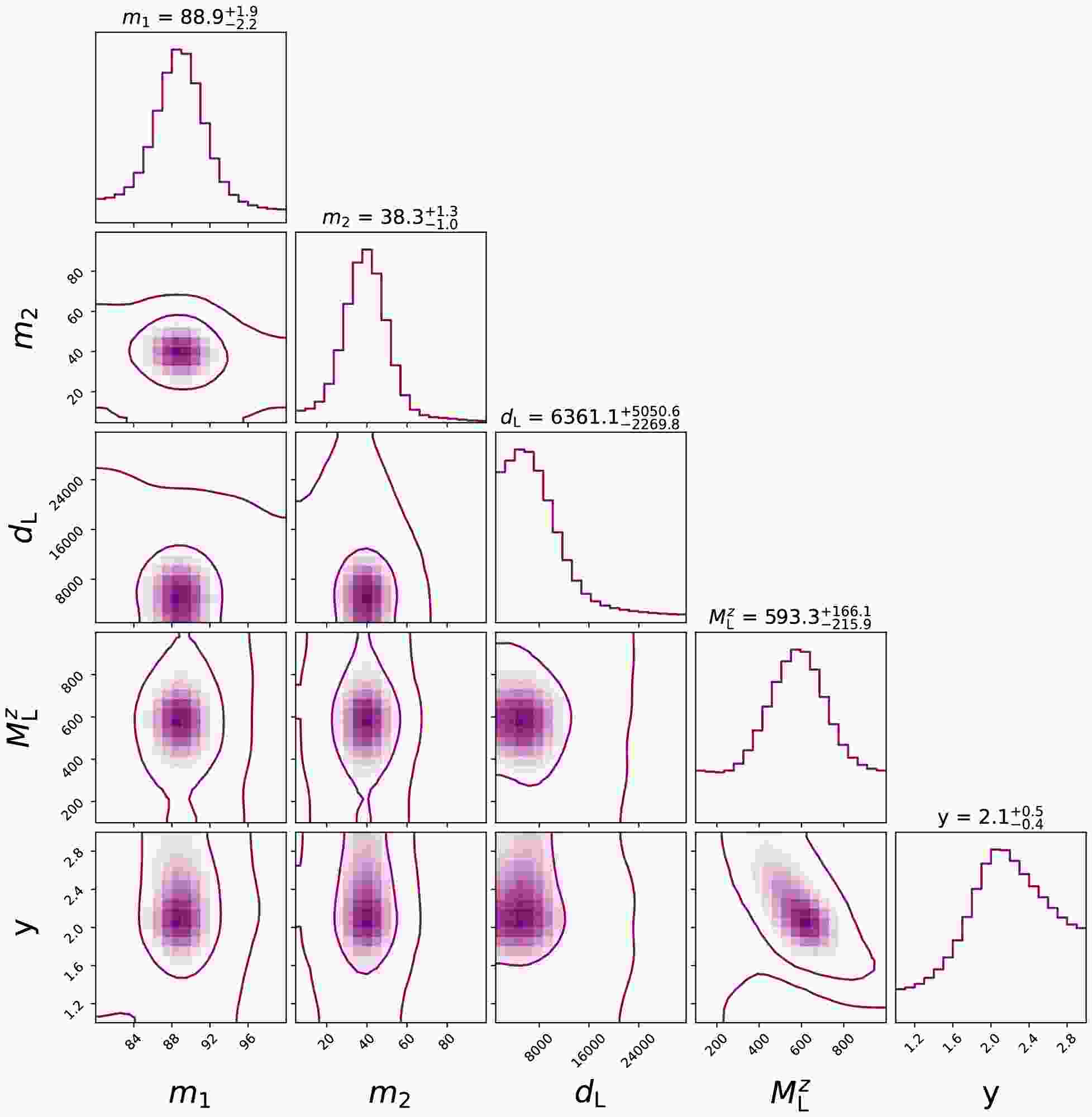
where $ \bar{h}(\theta) $ represents the microlensed GW waveform model. In the parameter estimation, we sample all source and lens parameters, together with the nuisance parameters mentioned above. The posterior distributions are obtained using the dynamic nested sampler implemented in $ \mathtt{dynesty} $, with the random-walk sampling method. We adopt zero-noise injections; i.e., the simulated data contain the lensed waveform without additional detector noise realizations.

Among the 10⁴ simulated BBH GW events, we identify eight detectable microlensed GW signals. The posterior distributions of the parameters for these events are shown in Fig. 1. In the right panel of Fig. 1, we compare the injected values of the GW source luminosity distance and the redshifted lens mass with their corresponding posterior estimates. The recovered values are consistent with the injected values within the $ 2\sigma $ credible regions, demonstrating the reliability of the parameter reconstruction.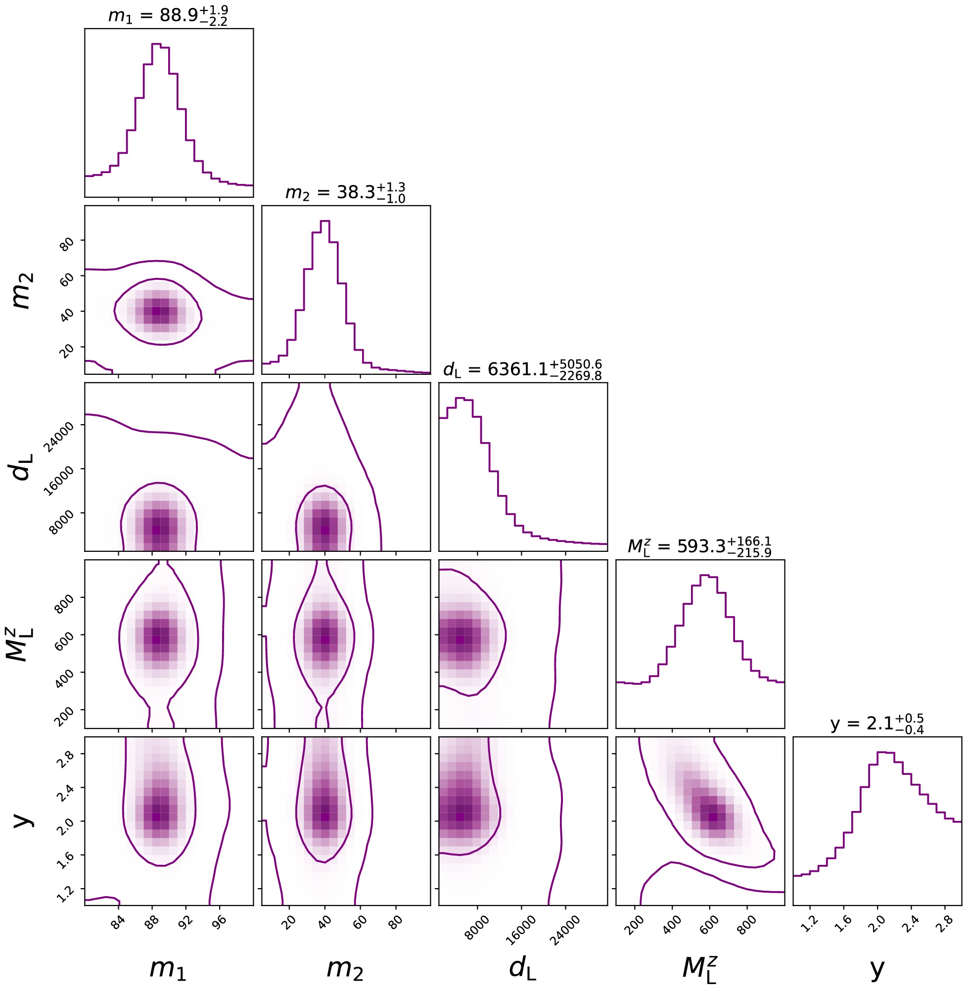

Figure 1.  (color online) Left: Posterior distribution for a representative event among the eight detectable microlensed GW events. Right: Comparison of the inferred and injected parameters for the eight detectable microlensed GW events. The crosses indicate the $ 2\sigma $ credible regions for the source luminosity distance and redshifted lens mass inferred from the posterior distributions, while the scattered points denote the corresponding injected values.

For the compact-DM population hyperparameters Φ and a set of $ N_{\rm{obs}} $ detected microlensing BBH events, $ d=\{d_1,\ldots,d_{N_{\rm{obs}}}\} $, with $ N_{\rm{obs}}=8 $ obtained from the 10⁴ simulated GW events in Section III, the population likelihood can be described by an inhomogeneous Poisson process. When measurement uncertainties are neglected and the selection effect is encoded in the expected number of detections $ N(\Phi) $, the likelihood is given by

Here, $ p_{\rm{pop}}(d_i|\Phi) $ denotes the probability of observing the i-th event under the population model characterized by the hyperparameters Φ. If the measurement uncertainty in the event-level parameters is neglected, this term is given directly by the population distribution in Eq. (26). When measurement uncertainties are included and selection effects are accounted for through the expected number of detections $ N_{\rm{det}}(\Phi) $, the likelihood for a set of $ N_{\rm{obs}} $ microlensed GW observations can be written as [86−88]

where $ {\cal L}(d_i|m_{\rm{L}}) $ denotes the single-event likelihood for the i-th microlensing GW event. This likelihood is obtained from single-event parameter estimation and is related to the posterior distributions $ p(M_{\rm{L}}^z|d_i) $ and $ p(d_{\rm{L}}(z_{\rm{S}})|d_i) $ via the priors adopted in the single-event analysis; for example, $ {\cal L}(d_i|M_{\rm{L}}^z)\propto p(M_{\rm{L}}^z|d_i)/\pi(M_{\rm{L}}^z) $. Here, $ N(\Phi) $ denotes the total number of microlensing events predicted by the population model characterized by the hyperparameters Φ.

where $ \chi(z_{\rm{L}}) $ is the comoving distance. The quantities $ N_{\rm{S}} $ and $ P_{\rm{S}}(z_{\rm{S}}) $ denote, respectively, the number of detectable GW sources and their redshift distribution. The comoving number density of compact DM objects with an extended mass distribution $ \psi(m_{\rm{L}},\gamma) $ is given by

where $ \rho_{\rm{c}} $ denotes the critical density of the Universe. The hyperparameters of the compact DM population are defined as

The lensing cross section in Eq. (28) is

We set the maximum impact parameter to $ y_0=5 $, because microlensing signatures become difficult to identify for $ y_0>5 $ [67, 69]. The normalized lens-mass distribution is then

The number of detectable GW microlensing events is defined as

where $ \sigma_{\rm{det}}(\lambda,m_{\rm{L}},z_{\rm{L}},z_{\rm{S}}) $ denotes the detection cross section for microlensing signals that satisfy the criterion in Eq. (23). It is given by

where $ \lambda\in[M_{\rm{L}}^{z},z_{\rm{S}},m_1,m_2,\ldots] $ denotes the relevant set of source and lens parameters. Therefore, the fraction of detected microlensed GW events is defined as

Finally, the posterior distribution of the population hyperparameters is derived from

where $ p(\Phi) $ denotes the prior distribution over the population hyperparameters, and $ Z_{{\cal{M}}} $ is the normalization constant (equivalently, the Bayesian evidence) for the population model $ {\cal{M}} $.

The selection effects in gravitational-lensing systems and the uncertainties in the inferred lens masses are shown in Fig. 2. Specifically, the left panel of Fig. 2 presents the detectable fraction of lensed GW events as a function of the power-law index. Our analysis reveals a positive correlation between the power-law index and the detection rate of microlensed GW events. This trend is physically expected: larger values of γ correspond to a higher abundance of massive lenses, which typically produce stronger lensing signatures and, consequently, higher SNRs. In the right panel of Fig. 2, we compare the inferred lens masses with the injected values used in the simulations. For each microlensed GW event, the parameter estimation provides joint posterior samples of the source luminosity distance $ d_{\rm{L}}(z_{\rm{S}}) $ and the redshifted lens mass $ M_{\rm{L}}^{z} $ from the MCMC chains. These samples preserve the correlation between $ d_{\rm{L}}(z_{\rm{S}}) $ and $ M_{\rm{L}}^{z} $. In the hierarchical inference, we use this two-dimensional joint posterior, rather than the product of the corresponding one-dimensional marginalized posteriors, and combine it with the optical-depth formalism in Eq. (27) to derive the lens-mass likelihood $ {\cal L}(d_i|m_{\rm{L}}) $ for each microlensed GW event. The results show that the inferred lens masses are consistent with their injected values within the $ 2\sigma $ credible regions.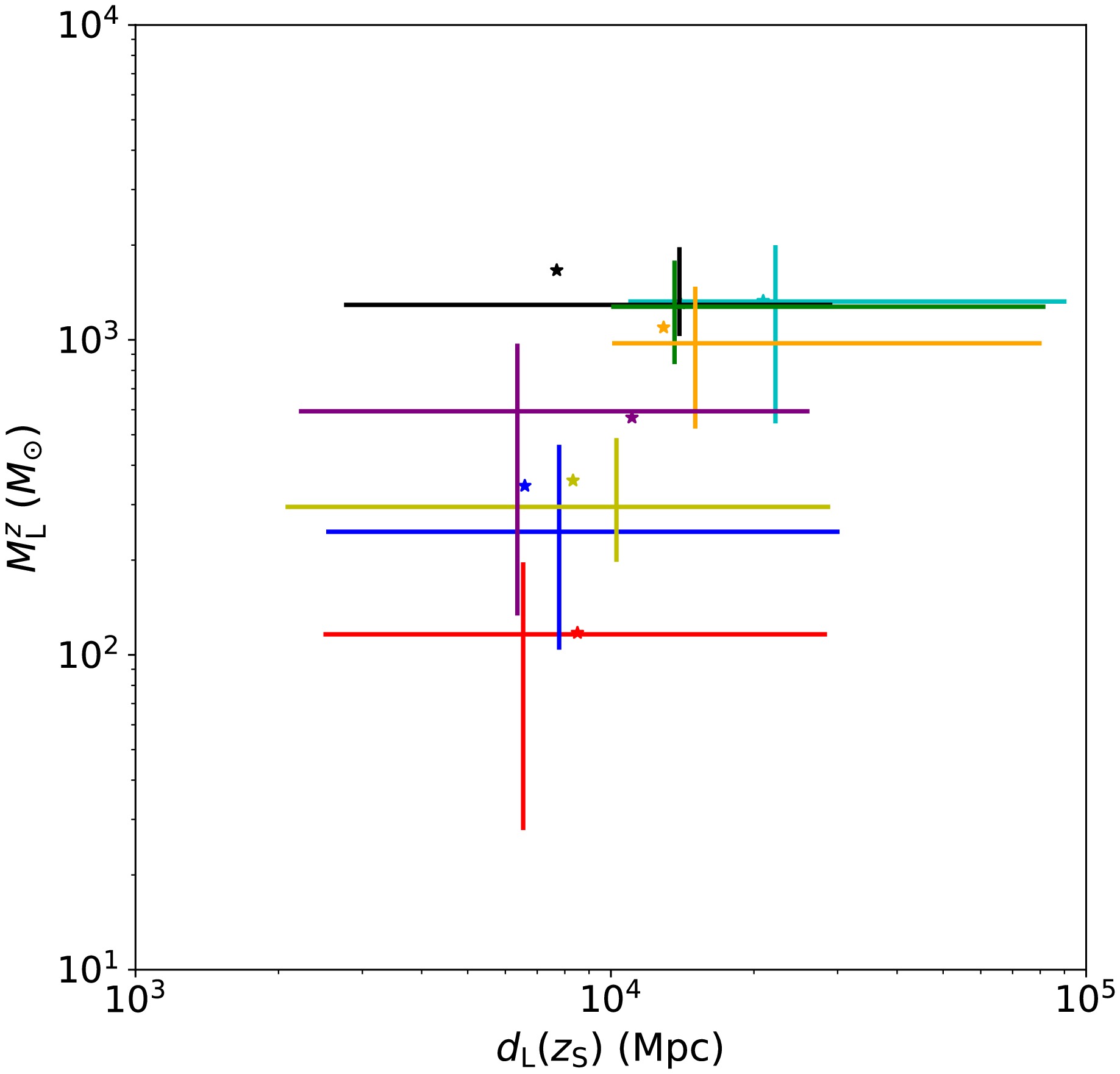

Figure 2.  (color online) Left: Detectable fraction of microlensed GW events, defined in Eq. (35). The blue points represent the simulation results, and the solid red curve shows the corresponding polynomial fit. Right: Inferred lens masses for the eight detectable microlensed GW events. The solid lines with points indicate the median values and 95% credible intervals obtained from the posterior distributions of the redshifted lens mass, $ p(M_{\rm{L}}^{z}|d_i) $, and the GW-source luminosity distance, $ p(d_{\rm{L}}(z_{\rm{S}})|d_i) $, shown in Fig. 1. The star markers denote the injected lens masses used in the simulations.

For the compact-DM population hyperparameters, we inject $ \gamma=1 $ and $ \log_{10}f_{\rm{CO}}=-2.5 $ in the simulation. This choice is not intended to represent a unique compact-DM formation scenario. Rather, it provides a simple illustrative case for testing whether the hierarchical Bayesian framework can recover the injected compact-DM population parameters. We aim to reconstruct γ and $ f_{\rm{CO}} $ from the inferred lens-mass distribution. For the priors, we fix the minimum and maximum masses in the mass function to $ M_{\min}=10\,M_{\odot} $ and $ M_{\max}=10^3\,M_{\odot} $, respectively. We adopt uniform priors on the power-law index and the compact-DM abundance, $ \gamma\in{\cal{U}}[-1,3] $ and $ \log_{10}(f_{\rm{CO}})\in{\cal{U}}[-4,-1] $, in Eq. (36). We then use the eight inferred lens masses from the microlensing GW events as input to $\mathtt{emcee} $ [89] and sample from the posterior distribution in Eq. (36) to infer the population hyperparameters $ \Phi\equiv\{\gamma, f_{\rm{CO}}\} $. The resulting constraints are shown in Fig. 3. We find that the best-fit values and 68% credible intervals are $ \gamma=0.41^{+0.42}_{-0.37} $ and $ \log_{10}(f_{\rm{CO}})=-2.76^{+0.16}_{-0.17} $. The blue marker in Fig. 3 denotes the injected hyperparameters used in our simulations, $ \Phi_{\rm{inj}}\equiv\{\gamma=1,\log_{10}(f_{\rm{CO}})=-2.5\} $. Our posterior constraints are consistent with the injected values within the $ 2\sigma $ credible region.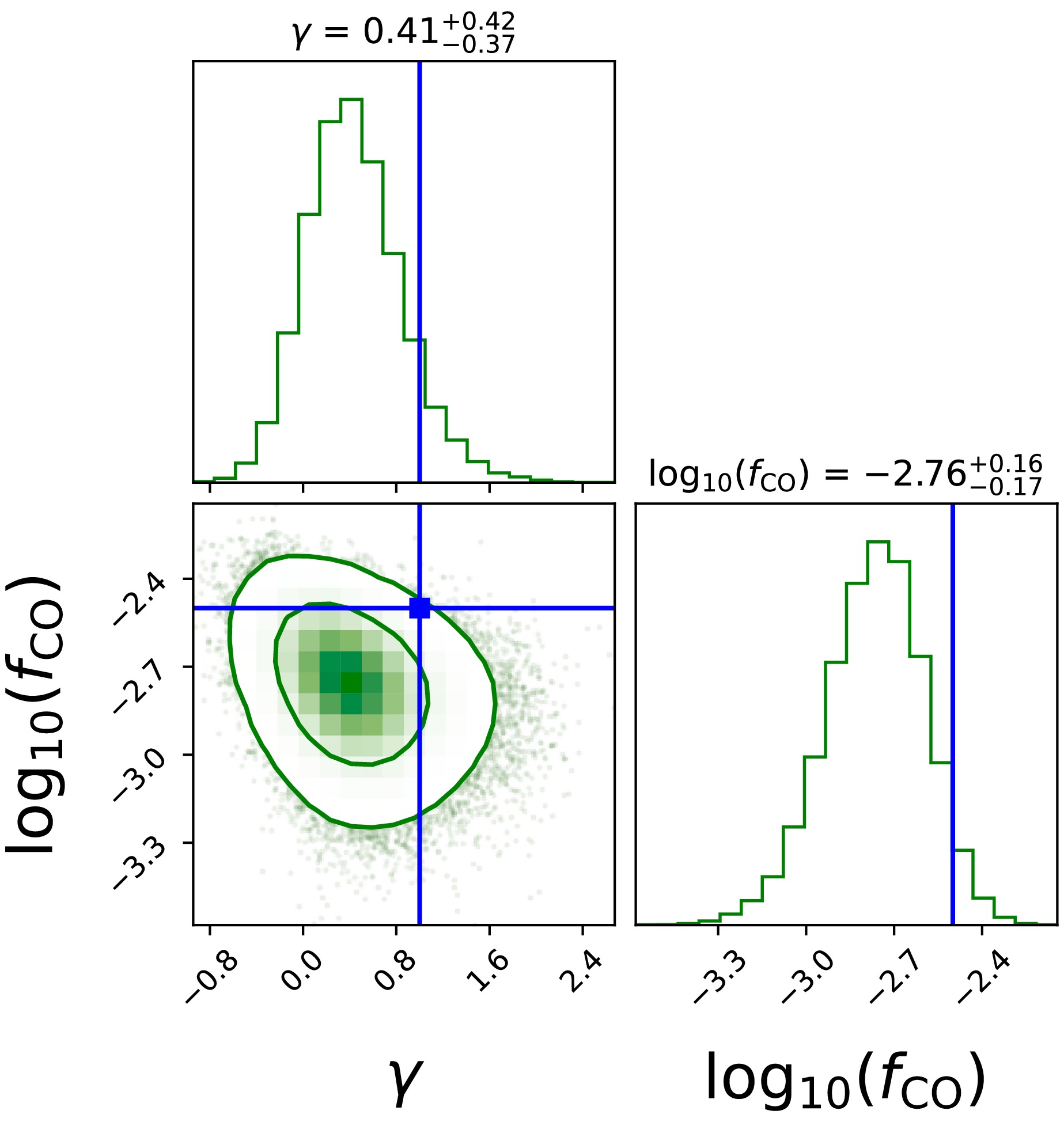

Figure 3.  (color online) Posterior distributions of the population hyperparameters $ [\gamma,\log_{10}(f_{\rm{CO}})] $; the $ 2\sigma $ credible region is shown. The solid blue point indicates the injected hyperparameter values used in our simulations, $ [\gamma=1,\log_{10}(f_{\rm{CO}})=-2.5] $.

In this paper, we present a comprehensive methodology for simulating GW events lensed by compact DM objects, extracting source and lens information from individual microlensing GW events, and constraining the population properties of compact DM objects using an ensemble of such events. Specifically, using the Einstein Telescope (ET) as a representative third-generation ground-based GW detector and modeling the lenses as point masses, we infer the posterior distributions of the GW-source and lens parameters for eight detectable microlensing GW events identified among 10⁴ simulated BBH mergers. Within a hierarchical Bayesian framework, we show that, for a compact DM population described by a power-law mass function, these eight microlensing GW events constrain the power-law index and compact DM abundance to $ \gamma=0.41^{+0.42}_{-0.37} $ and $ \log_{10}(f_{\rm{CO}})=-2.76^{+0.16}_{-0.17} $, respectively, at the 68% credible level, as shown in Fig. 3. The inferred constraints are consistent with the injected values used in the simulations at the $ 2\sigma $ level. The mild offset between the recovered and injected hyperparameters is expected because our theoretical prediction for the injected population suggests that more than ten microlensing GW events should be detectable, whereas only eight such events are identified in the simulated sample. This lower-than-expected number of detections naturally shifts the inferred constraints toward smaller values of both $ f_{\rm{CO}} $ and γ. Our primary aim is to demonstrate that, once a small sample of microlensing GW events is available, hierarchical Bayesian inference can, in principle, recover information on both the compact DM abundance and the shape of its mass function.

The methodology developed in this work represents a proof-of-principle step toward using future microlensing GW detections to infer compact DM population properties. It enables the extraction of compact DM population information from detected microlensing signatures and provides a pathway for probing the fundamental nature of compact DM, whether in the form of primordial black holes, exotic compact objects, or other non-particle dark-matter candidates. Although our method establishes a preliminary framework for constraining compact DM with future GW observations, several additional effects should be incorporated to describe the underlying physical processes more realistically:

● In this work, we have focused exclusively on the point-mass lens model. However, compact DM objects in the Universe may also occur in extended halo configurations, such as "dressed PBHs" [90−94]. If an observed signal is genuinely caused by microlensing, analyzing it with an incorrect lens model may bias parameter inference. Therefore, once a microlensed GW event is detected, accurately identifying the appropriate lens model will be crucial [62, 77].

● A complementary issue arises when an unlensed waveform is spuriously interpreted as a microlensing signal. For example, a GW signal from an eccentric binary may be misidentified as microlensed if analyzed using quasi-circular waveform templates. In such cases, lensing analyses may incorrectly attribute waveform modulations caused by orbital eccentricity to microlensing effects. Additional diagnostics, such as those based on the Kramers–Kronig (KK) relation [95, 96], are therefore required to resolve such degeneracies with lens parameters.

● To date, no definitive microlensing signature has been identified in any observed gravitational-wave event. Future detections will require more comprehensive waveform models to robustly interpret possible deviations from standard unlensed waveforms and to quantify the microlensing contribution from known stellar populations [97−101]. Ultimately, determining whether DM substructures can be reliably distinguished from the microlensing effects of known baryonic matter remains an important open challenge.

Constraints on compact DMs are expected to improve significantly as the number of GW microlensing detections increases rapidly in future surveys and the detection horizon of next-generation GW detectors expands. This progress will create substantial overlap between the parameter space probed by GW observations and that constrained by electromagnetic observations. Consequently, combining these two powerful multi-messenger probes will enable joint constraints on both the abundance and mass distribution of compact DMs. Such joint analyses are expected to play an important role in uncovering the nature of compact DMs and their formation mechanisms, thereby providing valuable insights into the physics of the early Universe.