Optimization of the factorization scale in QED Drell-Yan-like processes

Current and future high-precision experiments challenge theory by requiring highly accurate predictions, which in particular necessitate the calculation of higher-order contributions within perturbation theory. Precise theoretical predictions for radiative corrections to electron–positron annihilation are important for experiments at future electron–positron colliders, including FCC-ee [1] and CEPC [2]. Despite substantial progress in the development of multi-loop computational methods, computing the full $ {\cal{O}}(\alpha^2) $ electroweak and even QED radiative corrections to realistic observables in high-energy physics remains a complex task. The QED structure function ¹ approach [3] circumvents this problem by systematically accounting for higher-order contributions enhanced by powers of the so-called large logarithm.

where $ \mu_F $ is the factorization scale and $ \mu_R $ is the renormalization scale. Here, we consider the perturbative expansion of radiative corrections as a double series in α and the large logarithm. Terms of order $ {\cal{O}}(\alpha^n L^n) $ are usually called leading logarithmic (LL) contributions, whereas those of order $ {\cal{O}}(\alpha^nL^{n-1}) $ are next-to-leading logarithmic (NLL) contributions, and so on. Recently, NNLL electron and photon PDFs were calculated to $ {\mathcal O}(\alpha^2) $ order [4, 5].

The renormalization scale in QED is usually chosen to be equal to the electron mass $ m_e $; therefore, in what follows, we use $ \alpha(\mu_R^2)\equiv\alpha\approx\alpha(0) $. This choice is dictated by the need to explicitly define and control terms that are singular in the electron mass. By contrast, the choice of the factorization scale is not unique. Known explicit analytic results indicate that the factorization scale should correspond to the characteristic energy scale of the process under consideration. For example, choosing the factorization scale to be equal to the t-channel momentum transfer, $ \mu_F=\sqrt{-t} $, is reasonable for small-angle Bhabha scattering [6]. It should be borne in mind that the final result for a (renormalization-invariant) observable quantity, calculated to all orders in α and L, should not depend on the choice of either the renormalization or factorization scale. Moreover, for any fixed order in α, the sum of all contributions with different powers of L should not depend on the value of the factorization scale. Varying the factorization scale redistributes contributions among terms with different powers of L along the horizontal lines of the following formal representation of radiative corrections:

Optimization of the scale choice should help concentrate most of the corrections in terms with higher powers of the large logarithms, i.e., the LL and NLL terms. At the same time, we aim to reduce the contributions of terms with lower powers of L and higher powers of α, which are more difficult to calculate. In this way, we seek to improve the convergence of perturbative calculations and reduce the theoretical uncertainty associated with unknown higher-order terms.

Here, we consider the specific case of electron-positron annihilation into a virtual photon or Z boson. This process can be treated in exactly the same way as the Drell-Yan process in QCD, with factorization between parton density functions (PDFs) in the initial state and the hard subprocess; see ref. [7] for details. We now have a unique opportunity to quantitatively analyze the structure of representation (2), since the $ {\cal{O}}(\alpha^2L^0) $ contribution and many higher-order LL and NLL terms have been calculated analytically. Note that there is practically no other high-energy process for which an analytically known differential distribution is available in such detail.

The article is organized as follows. In the next section, we discuss the application of several approaches to choosing the factorization scale. The section is divided into three parts. In the first part, we compare the differential distributions obtained with three different factorization scales. In the second part, we analyze the effects of varying the factorization scale in the total cross section. In the third part, we test the effectiveness of the standard scale variation procedure ($ \mu_F \to \mu_F/2,\ 2 \mu_F $), which is commonly used to estimate uncertainties due to scale dependence. The final section contains concluding remarks.

In this article, we systematically compare $ \mu = \sqrt{s} $, $ \mu = \sqrt{sz} $, and $ \mu = \sqrt{s/e} $, where $ e \approx 2.71828 $ is Euler's number, and perform a quantitative test of the LL and NLL approximations against the known complete $ {\cal{O}}(\alpha^2) $ result. We also study the reliability of the conventional factor-of-two factorization-scale variation and observe that this variation can underestimate the uncertainty when radiative return to lower energies is enhanced.

Many methods are known for optimizing the choice of factorization scale; see, e.g., [8]. In the conventional scale setting (CSS) scheme, $ \mu_F $ is chosen to be equal to the characteristic energy scale of the hard subprocess: for example, the invariant mass of the final-state lepton pair in Drell-Yan-like processes at the LHC [9] and the muon mass for the muon decay spectrum [10]. However, this approach has several drawbacks. Some processes may involve more than one characteristic scale (e.g., in large-angle Bhabha scattering, amplitudes occur in the s, t, and u channels), and the results can also depend on the choice of renormalization scale and scheme.

The method of fastest apparent convergence (FAC) [11] exploits the notion of effective charges. A similar approach was also proposed by N.V. Krasnikov [12]. The basic idea is that an effective charge can be associated with a given physical quantity, and higher-order corrections to that quantity can be absorbed by renormalizing the charge, so that the LL-corrected expression is equal to the sum of the LL and NLL corrections [13]. In the case of differential distributions, and when anomalous dimensions contribute to the physical quantity of interest, the FAC method suggests choosing the value of $ \mu_F $ that corresponds to the fastest convergence of the series of results obtained in the LL, NLL, NNLL, and higher approximations.

The Brodsky-Lepage-Mackenzie (BLM) [14] procedure is based on the resummation of vacuum polarization effects in the running coupling constant. The optimal renormalization and factorization scales for a particular process at a given order can be determined by computing the vacuum polarization parts of the diagrams at that order and setting the scale at which the terms proportional to the number of flavors $ N_f $ are absorbed into the coupling constant. The principle of maximal conformality (PMC) [15, 16] is a generalization of the BLM prescription to all orders and different types of observables. This approach aims to make the results of perturbative calculations invariant with respect to the choices of renormalization scale and scheme. The main idea is to exploit renormalization group invariance. As a result, the convergence of the perturbative QCD series can be improved. It should also be noted that applying the PMC approach requires careful consideration of higher-order effects [17, 18, 19].

The principle of minimal sensitivity (PMS) was proposed by P.M. Stevenson [20]. According to this principle, the optimal factorization scale is the one for which the result is least sensitive to the value of the scale. In PMS, the scale can be chosen by setting the derivative of the physical quantity of interest with respect to the factorization scale to zero (or to its apparent minimum value).

Our goal here is to analyze the applicability and effectiveness of various scale selection prescriptions for a specific QED process in which analytical results are known for several orders in α and L.

We consider the process of electron–positron annihilation.

where $ (n \gamma,e^+e^-) $ denotes the possible emission of photons and/or $ e^+e^- $ pairs.

The contribution to the cross section for this process from one-loop initial-state radiation (ISR) corrections is given by [21]

where the standard plus prescription is applied and $ \zeta(2)=\pi^2/6 $. The corresponding complete two-loop result was presented in [21] and corrected in [22]. These results can be compared with those obtained using the QED structure-function approach [3] in the next-to-leading logarithmic approximation [7, 23]. In this approach, the cross section is represented in Drell–Yan form

where $ D^{\mathrm{str}}_{ie}(x,\mu_R^2/\mu^2_F) $ are the electron structure (parton density) functions [3, 24, 25]. The lower integration limits $ \bar{z}_{1,2} $ for the energy fractions depend on the experimental conditions. In the term $ D \otimes D\otimes\sigma^{(0)} $, $ z \equiv z_1z_2 $, and $ sz $ is the square of the observed invariant mass of the final-state muon pair. Expanding this master formula to first order in α gives

where

and "$ + $" denotes the plus prescription, and $ \bar{\sigma}^{(1)}_{\bar{e} e} $ is the one-loop contribution to the annihilation subprocess cross section for massless partons, computed within the $ \overline{\mathrm{MS}} $ scheme for the subtraction of electron mass singularities. It is convenient to choose $ \mu_R=m_e $ so that logarithms of different energy-scale ratios are collected in one place, i.e., to define the large logarithm as $ L=\ln(\mu_F^2/m_e^2) $. It should also be noted that choosing $ \mu_R = \mu_F $ would completely eliminate the benefit of using the structure function method in QED, since all large logarithms would vanish and large contributions would shift to terms of order $ {\cal{O}}(\alpha^nL^0) $, which are very difficult to calculate. Note also that the left-hand side of Eq. (6) does not depend on $ \mu_F $, so the dependence on this parameter cancels on the right-hand side between the first term in the square brackets and $ \bar{\sigma}^{(1)}_{\bar{e} e} $. Moreover, the cancellation of the $ \mu_F $ dependence occurs in each line of Eq. (2) (starting from the second one).

One can take $ \mu_F^2 = s $ as the first option for the factorization-scale choice, so that $ L=\ln(s/m_e^2) $. Another option is adopted in Refs. [21] and [23, 26], where $ \mu_F^2 = s z $ is chosen; thus, the factorization scale is equal to the invariant mass of the final $ \mu^+\mu^- $ system, and the large logarithm is $ \hat L = L + \ln z $. Note that in the latter case, the factorization scale is equal to the energy transfer of the hard subprocess, i.e., the CSS prescription is applied.

The master equation (5) for the cross section can be expanded as

Higher-order coefficients $ c_{kl}(z) $ in the leading and next-to-leading logarithmic approximations through $ c_{65} $ were first calculated in [23], and some of these coefficients were independently recalculated and corrected in [7]. Explicit expressions for the additions to $ c_{20} $ relative to the result in Berends' work [21] can be found in [22]. For convenience, we present the explicit result in the Appendix.

A change in the factorization scale, and the corresponding change in the large logarithm, leads to a redistribution of contributions at each order in α. Let us now consider radiative corrections of order $ {\cal{O}}(\alpha^2) $. Any change in the factorization scale must not change the full correction at a given order in α (or the complete result for the cross section):

where we denote

We treat changes in the factorization scale as an additive contribution to the large logarithm:

and we get the matching equality:

We obtain expressions for the new coefficients $ \hat{c}_{ij} $:

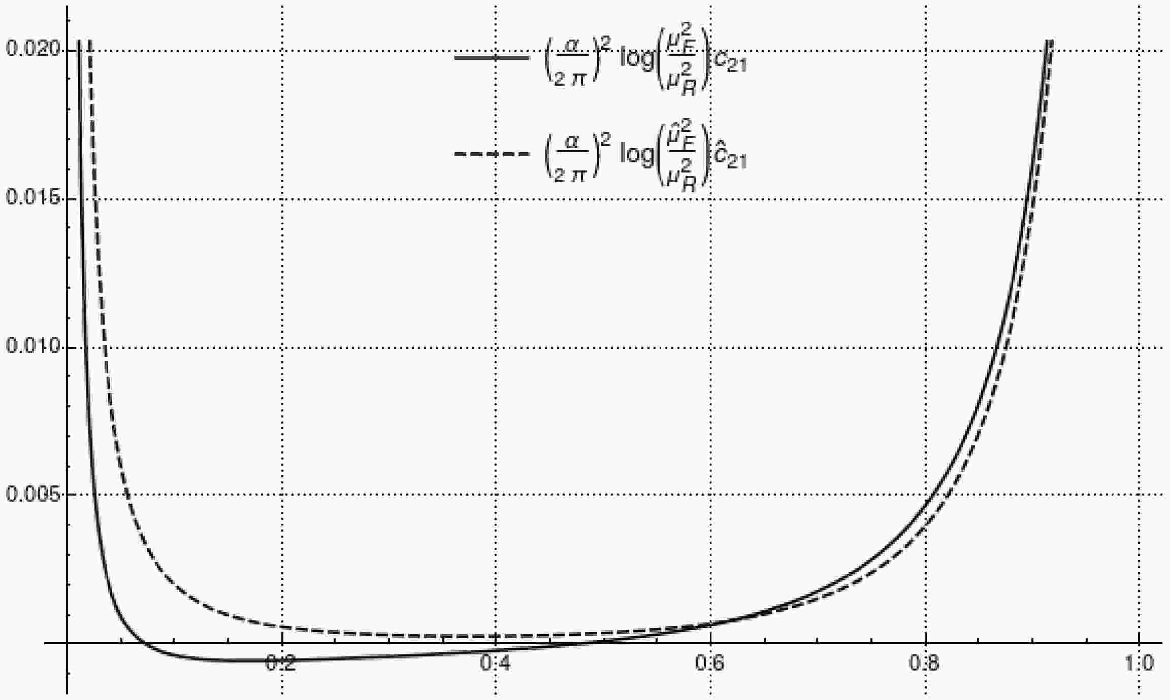
The behavior of the functions $ c_{ij}(z) $ for $ \mu_F=\sqrt{s} $ and $ \hat{c}_{ij}(z) $ for $ \hat{\mu}_F=\sqrt{sz} $ at order $ {\cal{O}}(\alpha^2) $ is shown in Figs. 1 and 2. As $ z\to 0 $, the functions increase rapidly because of terms proportional to $ 1/z $ and $ \ln(z) $, which are associated with the singlet pair-production mechanism. If necessary, these terms can be resummed within the Balitsky-Fadin-Kuraev-Lipatov (BFKL) formalism [27]. The peaked behavior as $ z\to 1 $ is governed by soft photon and pair emission and is regularized by the corresponding terms arising from virtual radiative corrections. For more details, see [7].

Figure 1.  $ {\cal{O}}(\alpha^2L^1) $ contributions for different factorization scales as a function of the energy fraction z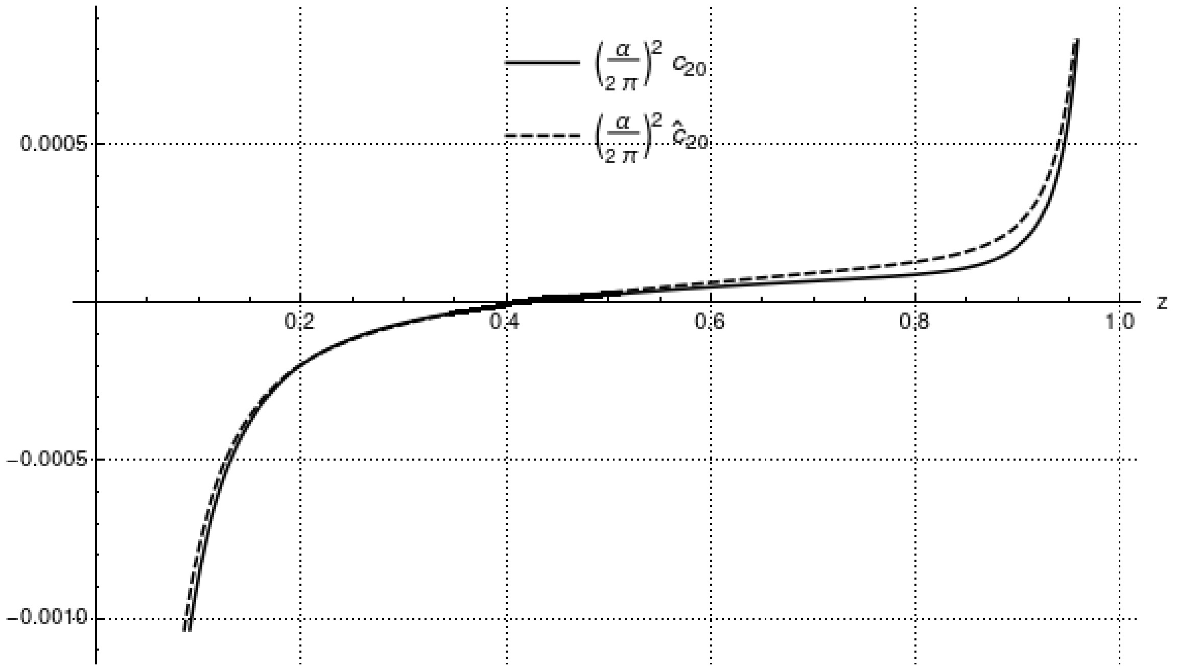

Figure 2.  Contributions at $ {\cal{O}}(\alpha^2L^0)$ for different factorization scales

At $ \sqrt{s}=240 $ GeV, radiative return to the Z resonance occurs at $ z \approx 0.14 $, where $ sz=M_Z^2 $. At $ \sqrt{s}=160 $ GeV, the Z resonance peak occurs at $ z \approx 0.32 $. We examine the contributions to the differential cross section at orders $ {\cal{O}}(\alpha) $ and $ {\cal{O}}(\alpha^2) $ for $ \sqrt{s} = 240 $ GeV. The interval from $ z=0 $ to $ z=1 $ is divided into 20 bins, and the integration is performed separately for each bin, starting from $ z_{min} = 0.05 $. The histograms for the cross section with two different factorization scales, $ \sqrt{s/e} $ and $ \sqrt{s z} $, denoted in the plots by "$ (L-1) $" and "$ (L+ \ln z) $", respectively, together with the differences from the total result for the correction at the given order, are shown in Figs. 3 and 5. In Fig. 4, the LL corrections at the $ \sqrt{s/e} $ and $ \sqrt{s z} $ factorization scales are compared with the LL+NLL contribution at the $ \sqrt{s} $ factorization scale. These values are shown as percentages relative to the Born cross section $ \sigma^{(0)}_{\bar{e}e}(s) $ [21]. Here, $ h_{i,tot} $ is the sum of all corrections of the given $ i^{\mathrm{th}} $ order in α, e.g.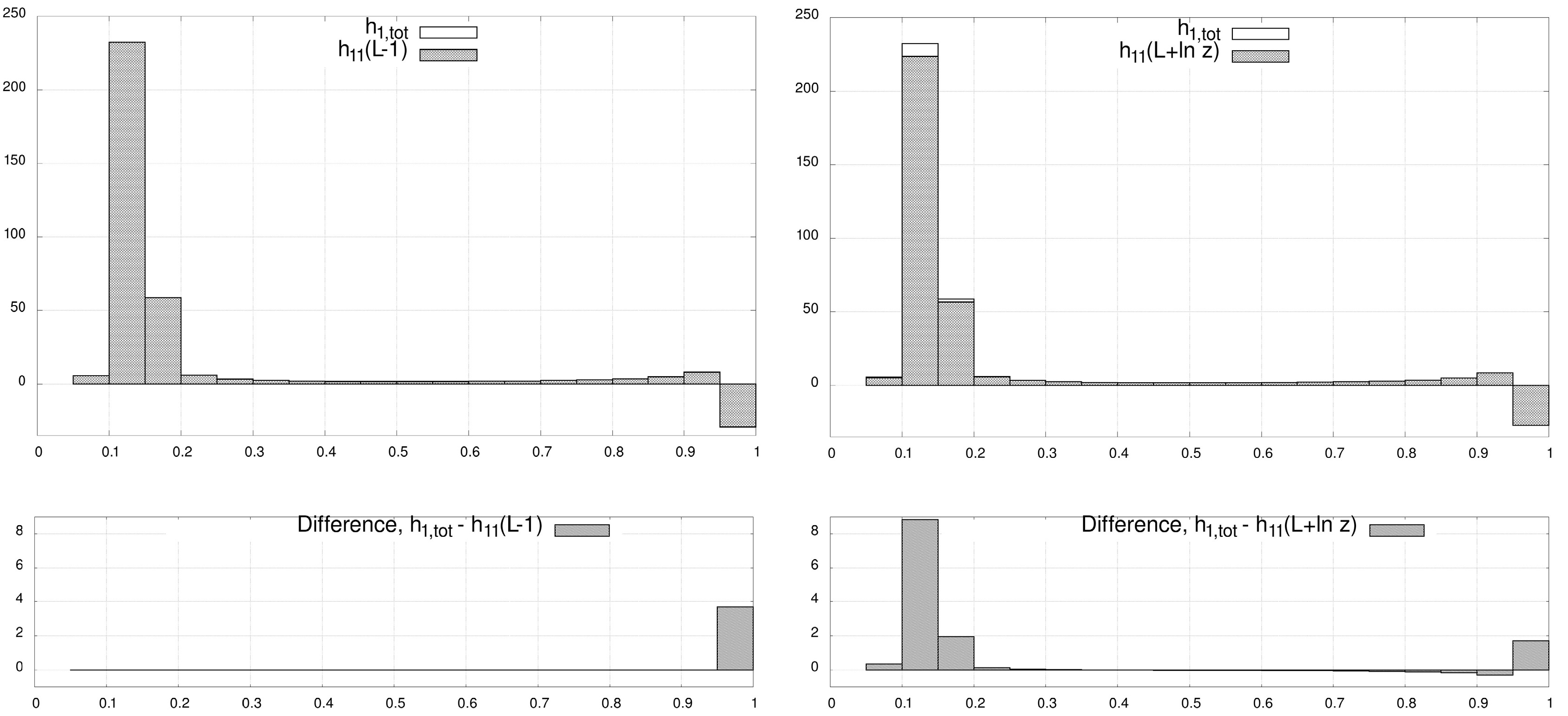

Figure 3.  First-order LL corrections and their differences from the complete LL+NLL result for two factorization scales, $ \sqrt{s/e} $ (left) and $ \sqrt{s z} $ (right), at $ \sqrt{s}=240 $ GeV, expressed as percentages, as functions of the energy fraction z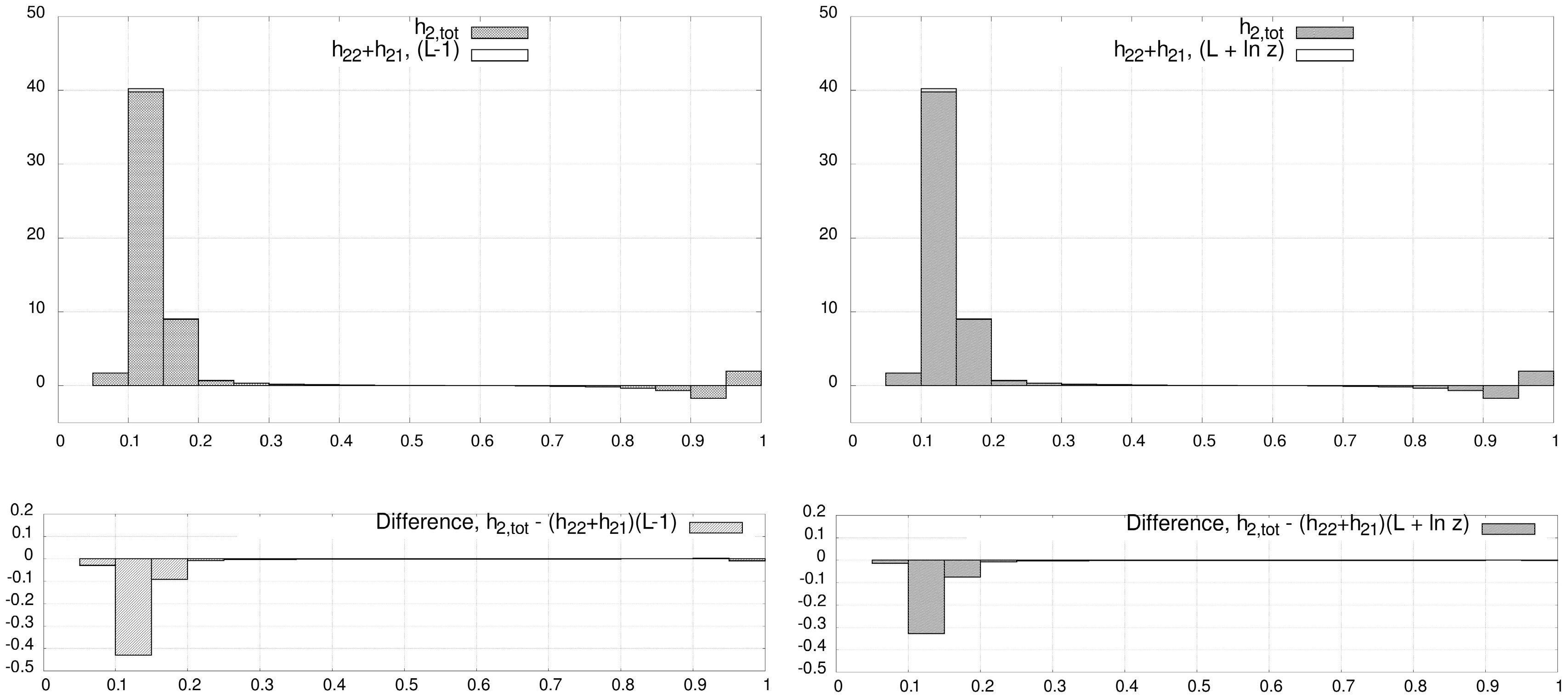

Figure 5.  Second-order NLL corrections and their differences from the full NNLL result for two factorization scales, $ \sqrt{s/e} $ (left) and $ \sqrt{s z} $ (right), at $ \sqrt{s}=240 $ GeV, expressed as percentages, as functions of the energy fraction z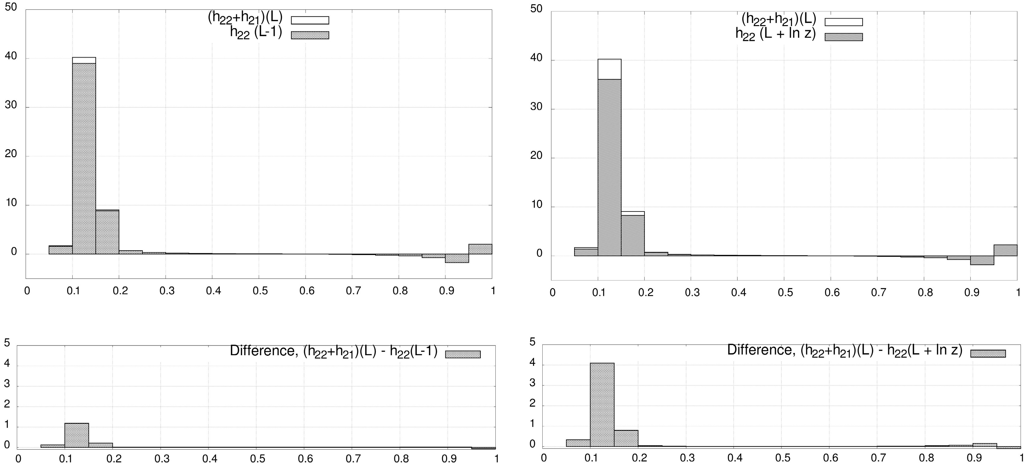

Figure 4.  Second-order LL corrections at two factorization scales, $ \sqrt{s/e} $ (left) and $ \sqrt{s z} $ (right), and their differences from the LL+NLL result at $ \mu_F=\sqrt{s} $ for $ \sqrt{s}=240 $ GeV, expressed as percentages, as a function of the energy fraction z

The preferred factorization scale appears to be $ \sqrt{s/e} $, because at order $ {\cal{O}} (\alpha^1) $ the NLL contribution is almost completely absorbed into the LL contribution, except in the last bin; see Fig. 3. A similar situation occurs for the choice of the preferred factorization scale in the leading $ {\cal{O}}(\alpha^2L^2) $ contribution, which absorbs the bulk of the $ {\cal{O}}(\alpha^2L^1) $ effect for $ \mu_F=\sqrt{s/e} $, as shown in Fig. 4. However, at the NLL level, when considering the sum of the $ {\cal{O}}(\alpha^2L^2) $ and $ {\cal{O}}(\alpha^2L^1) $ corrections, Fig. 5 shows that for $ \mu_F=\sqrt{sz} $ most NNLL contributions are absorbed into the NLL contributions. Note that this occurs for the distribution integrated over bins and for the particular choice of the c.m.s. energy.

By integrating the corrected cross section from $ z_{min}=0.1 $ to $ 1 $ at $ \sqrt{s}=240 $ GeV, we include the contribution due to radiative return to the Z resonance in the integration domain, which yields unusually large corrections. Thus, at $ e^+e^- $ colliders with energies above the Z peak, one can expect a substantial number of events due to radiative return to the peak, and the theoretical uncertainties in the description of such events will be affected by large, as-yet unknown higher-order contributions.

Figs. 6 and 7 show the LL and NLL corrections as functions of the factorization scale choice with $ z_{min}=0.1 $. They are compared with the results obtained with the factorization scale $ \mu_F = \sqrt{sz} $; the corresponding lines are marked $ h_{ij} (L + \ln z) $. The center-of-mass (c.m.s.) energies are $ 240 $ GeV and $ 3 $ TeV, which correspond to the optimal energy for associated production of Higgs and Z bosons at FCC-ee and CEPC colliders and to the maximum energy of the CLIC collider project [29], respectively. The factorization scale is varied from $ 10 $ GeV to the maximum c.m.s. energy. The complete correction at a given order in α does not depend on the factorization scale. Figs. 6 and 7 show the $ {\cal{O}}(\alpha^1) $ and $ {\cal{O}}(\alpha^2) $ corrections with different scales for better readability. The figures show that the leading logarithmic contributions $ h_{11} $ and $ h_{22} $ depend strongly on $ \mu_F $, whereas at next-to-leading accuracy this dependence becomes rather weak. The conventional choice of the factorization scale $ \mu_F = \sqrt{sz} $ is certainly not optimal in the LL approximation, but it can work reasonably well in the NLL case. According to the principle of minimal sensitivity, the best factorization scale is the point at which the derivative of the function is zero. This approach does not work for the leading logarithmic approximation, since the dependence on $ \mu_F $ is monotonic. For $ h_{22}+h_{21} $, there is a maximum, which is situated at $ \mu_F \approx 175.6 $ GeV for $ \sqrt{s}=240 $ GeV and at $ \mu_F \approx 3.8 $ TeV for $ \sqrt{s}=3 $ TeV. However, the second-order correction $ h_{22}+h_{21} $ is almost flat, so the PMS approach does not appear to be very instructive, especially if additional uncertainties are present, e.g., due to non-perturbative effects in QCD. The FAC approach provides a clear and simple prescription for choosing the factorization scale at the intersection of the curves corresponding to the leading and next-to-leading approximations. This scale choice actually provides a quite reasonable approximation of the total $ O(\alpha^2) $ result.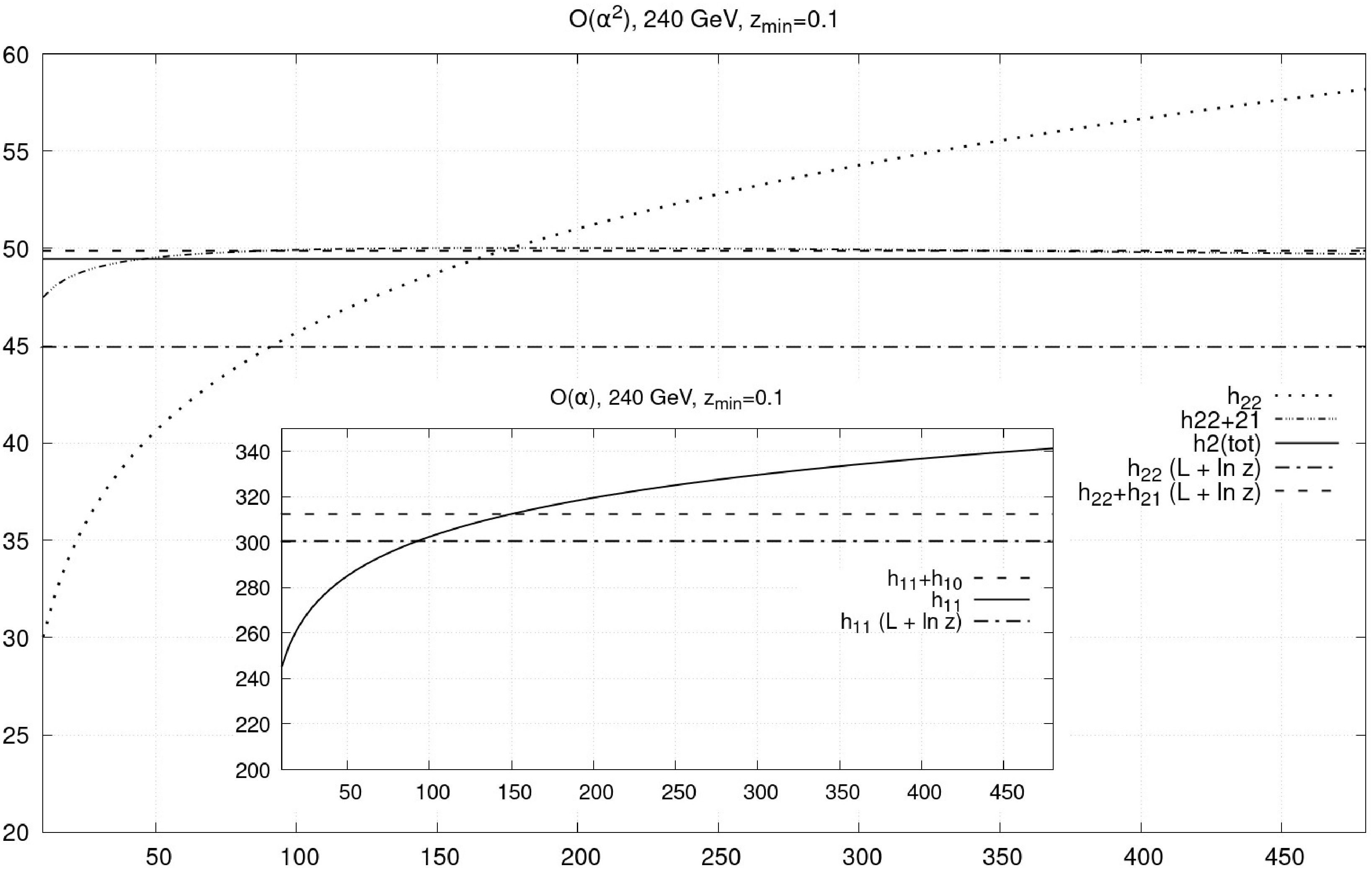

Figure 6.  Corrections as a function of the factorization scale at $ \sqrt{s}=240 $ GeV and $ z_{min}=0.1 $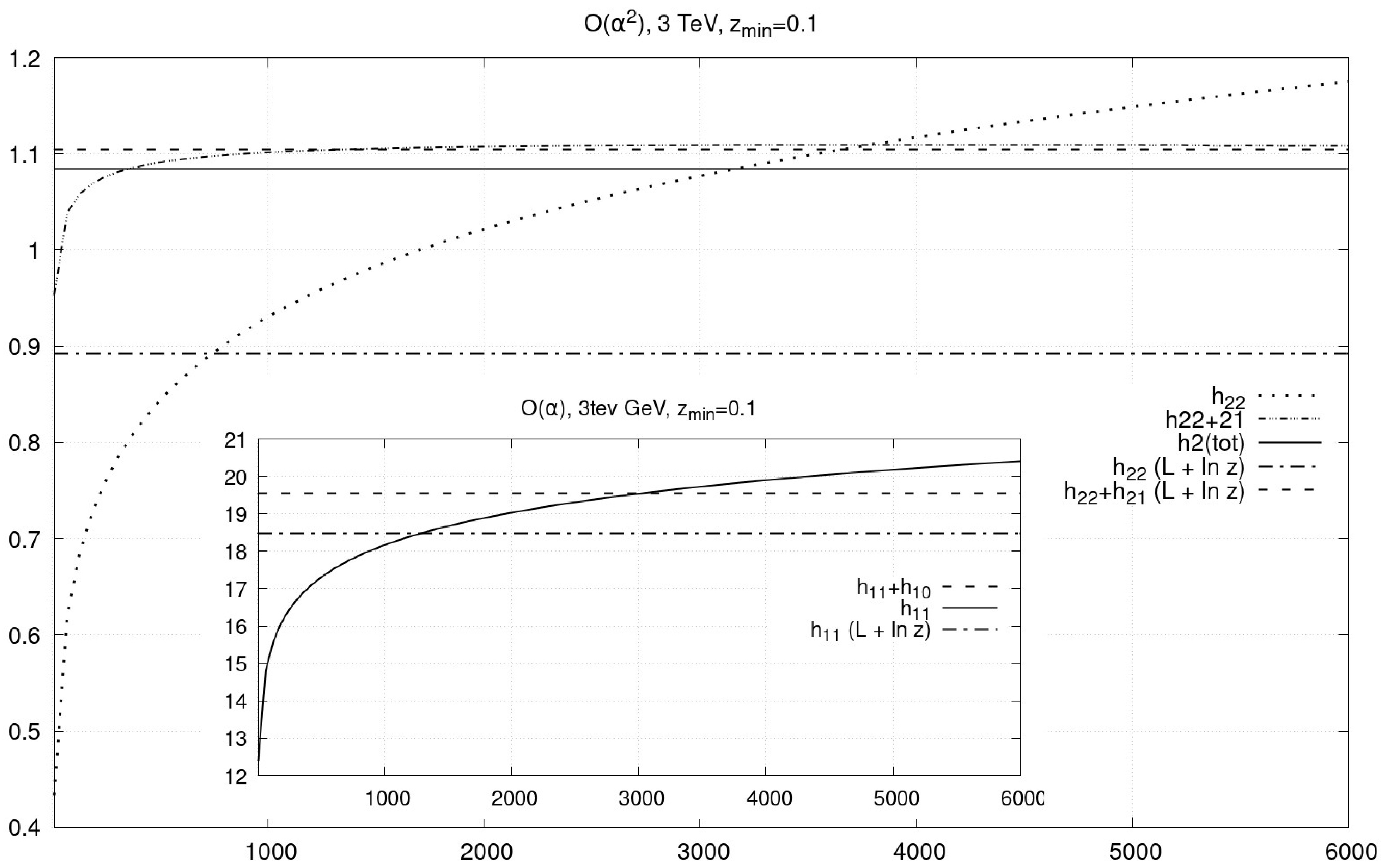

Figure 7.  Corrections as a function of the factorization scale at $ \sqrt{s}=3 $ TeV and $ z_{min}=0.1 $

Note that the difference between the NLL contribution $ h_{22}+h_{21} $ and the total $ O(\alpha^2) $ result is almost insensitive to the factorization scale choice. This means that this difference can hardly be absorbed into the factorization scale choice. The reason is that this difference mainly arises from contributions that are not proportional to those enhanced by large logarithms. In particular, we see that BFKL-like terms proportional to $ \ln^k(z)/z, \ \ k\geq 0 $ are numerically important when small z values are not excluded by experimental cuts.

It is reasonable to choose the factorization scale at the intersection of the LL and LL+NLL correction curves. This choice corresponds to the fastest apparent convergence prescription. At $ \sqrt{s}=240 $ GeV for the order $ {\cal{O}}(\alpha) $, the corresponding scale is about $ 150 $ GeV, which is close to $ \sqrt{s/e}= {240}/\sqrt{e}\approx146 $ GeV. Importantly, at higher orders, owing to the more complicated structure of the corrections, this intersection point is shifted. Moreover, the position of the intersection point depends on the experimental cuts, e.g., on $ z_{min} $. Thus, there can be no ideal choice of the factorization scale, but its optimization remains very important.

The numerical values of the corrections for different $ z_{min} $ are given in Table 1. The table presents the full $ {\cal{O}}(\alpha^2) $ corrections, the sum of the $ {\cal{O}}(\alpha^2L^2) $ and $ {\cal{O}}(\alpha^2L^1) $ contributions, and the $ {\cal{O}}(\alpha^2L^2) $ part separately for different factorization scale values. The corrections are significantly larger at $ z_{min}=0.1 $ than at $ z_{min}=0.5 $ because radiative return to the resonance is allowed in the former case. The corrections also increase at $ z_{min}=0.9 $ due to the soft radiation contributions. As expected, the full $ {\cal{O}} (\alpha^2) $ correction does not depend on the factorization scale value. For $ \mu_F=\sqrt{s/e} $, the LL result $ h_{22} $ is closer to the total sum $ h_{22}+h_{21}+h_{20} $, except in the case $ z_{min}=0.1 $ at $ \sqrt{s}=3 $ TeV, where $ \mu_F=\sqrt{s} $ works better. By contrast, in the NLL approximation, $ \mu_F=\sqrt{sz} $ works somewhat better. It can also be noted that, for $ z_{min}=0.1 $, the variation in the factorization scale among the three values under consideration substantially underestimates the difference between the NLL and NNLL results.

We now examine the effect of varying the factorization scale by a factor of 2. The magnitude of the corresponding effect is commonly used to estimate unaccounted-for higher-order corrections [30].

We choose the central value of the factorization scale $ \mu_F $ and compute $ h_{22} $, $ h_{22} + h_{21} $, and $ h_{33} $ at the factorization scales $ 2 \mu_F $ and $ \mu_F/2 $. In Eq. (16), $ \Delta_2^{LL} $ and $ \Delta_3^{LL} $ are $ h_{21} $ and $ h_{32} $, respectively, and $ \Delta_2^{NLL} $ is $ h_{20} $ at the central value of the factorization scale. Thus, $ \Delta_2^{LL} $, $ \Delta_3^{LL} $, and $ \Delta_2^{NLL} $ are the true values of the shifts due to ``unknown contributions'' when working in the LL and NLL approximations, respectively. The quantities $ \delta^{LL} $ and $ \delta^{NLL} $ show the average shifts of the LL and NLL contributions due to variation of the factorization scale. Thus, $ \delta_{LL,NLL} $ are the estimated shifts of the corresponding ``unknown contributions''. The true and estimated shifts are defined as follows:

where $ h_{ij}(2) $ and $ h_{ij}(1/2) $ are $ h_{ij} $ evaluated at factorization scales $ 2 \mu_F $ and $ \mu_F/2 $, respectively, and $ h_{ij} $ without an argument denotes $ h_{ij} $ at the initial (central) factorization scale. Numerical values of $ h_{ij} $ can be found in our work [28].

The numerical results for the shifts are given in Tables 2—4 for three different values of the factorization scale and three energies. The results show that the average LL shift is of the same order as the corresponding NLL contribution ($ h_{21} $ or $ h_{32} $). However, for the NLL at $ \sqrt{s} = M_z $, the variation of the factorization scale significantly overestimates $ h_{20} $ for $ \mu_F=\sqrt{s} $ and $ \mu_F=\sqrt{sz} $. At $ \sqrt{s} = M_z $, in both the $ {\cal{O}}(\alpha^2) $ and $ {\cal{O}}(\alpha^3) $ orders, Δ and δ change very little with variations in $ z_{min} $, since radiative return is not efficient in this case. However, at energies above the Z peak (for $ \sqrt{s}=240 $ GeV or 3 TeV) and for $ z_{min}=0.1 $, the estimated shifts $ \delta_2^{\mathrm{NLL}} $ and $ \delta_3^{\mathrm{LL}} $ substantially underestimate the corresponding actual values. Note that for $ \sqrt{s}=240 $ GeV at $ z_{min}=0.1 $, radiative return to the resonance is taken into account, whereas for $ \sqrt{s}=3 $ TeV it contributes only for $ z_{min}<0.001 $. Thus, radiative return occurs only to lower center-of-mass energies where the cross section is higher. For both $ \mu_F=\sqrt{sz} $ and $ \mu_F=\sqrt{s/e} $, the variation underestimates the actual NLL correction at $ \sqrt{s} = 3 $ TeV and $ z_{min}=0.1 $ because of QED BFKL effects at small z values ². Both scales are not optimal for $ 3 $ TeV. A better scale choice in this case can be obtained using the FAC and PMS approaches ($ \mu_F\approx 3.8 $ TeV).

We considered various options for choosing the factorization scale for corrections to the $ e^+e^- \rightarrow \gamma^*/Z^* $ processes. High-precision theoretical predictions for these processes are required for studies at future electron–positron colliders, including FCC-ee and CEPC. We observe that factorization-scale dependence constitutes a considerable source of uncertainty in estimates of higher-order corrections due to initial-state radiation.

Having examined known complete results at $ {\cal{O}}(\alpha) $ and $ {\cal{O}}(\alpha^2) $, we conclude that, for this process, high values of the factorization scale, of the order of the initial center-of-mass energy $ \mu_F\approx \sqrt{s} $, are preferable. This choice is consistent with the prescription provided by the fastest apparent convergence method. Application of the principle of minimal sensitivity also favors large $ \mu_F \sim \sqrt{s} $. The conventional scale-setting scheme yields $ \mu_F=\sqrt{zs} $, which is the momentum (energy) transfer in the hard subprocess. This scale choice completely fails in the leading-logarithmic approximation but works sufficiently well at NLL for the considered beam energies. It should also be noted that the BLM and PMC prescriptions are not applicable in our case, since the dominant scale dependence arises not from the running coupling constant but from the cusp anomalous dimensions.

We also verified the validity of the standard scale-uncertainty estimation procedure by varying the factorization scale by a factor of 2. We found that the procedure provides reasonable numerical estimates for some setups, but not for the crucial case of radiative return to a resonance or simply to lower energies of the hard subprocess. In the latter case, the standard method substantially underestimates the uncertainty.

Our results are relevant for developing an advanced treatment of higher-order QED corrections for electron–positron annihilation processes studied at current and future colliders. Our study was conducted for the case of pure QED, but pure QED can be viewed as an Abelian reduction of the Drell–Yan process in QCD, where the issue of scale dependence is also significant. Therefore, some of the presented insights into scale dependence may also be relevant for QCD, in particular for the description of Drell–Yan-like processes at the LHC.

The explicit expression for the NNLL correction at order $ {\cal{O}}(\alpha^2L^0) $ for $ \mu_F=\sqrt{s} $, compiled from the results of refs. [21, 22, 31], reads

Note that this result differs from that reported in [32].

We thank A.L. Kataev for fruitful discussions.

The data supporting the findings of this study are available from the authors upon reasonable request.