Analytic solution for the motion of spinning particles in plane gravitational wave spacetime

The motion of spinning test particles in curved spacetime plays a central role in many problems in general relativity. At the dipole level, the dynamics are governed by the Mathisson–Papapetrou–Dixon (MPD) equations [1, 2], which encode the coupling between the particle's intrinsic spin and the background curvature. This spin– curvature interaction generates corrections to geodesic motion, affecting precession and orbital phasing. Such effects are essential in a wide range of relativistic scenarios [3−11].

In many physically relevant situations, gravitational radiation can be accurately modeled as a plane gravitational wave. This description naturally emerges in the local wave zone of an isolated source, where the curvature radius of the wavefront is much larger than the scale of a detector or test body, rendering the wavefront locally planar. Moreover, plane wave spacetimes appear universally as Penrose limits [12] of arbitrary geometries taken along null geodesics, providing a powerful local description of the geometry experienced by highly boosted observers. These fundamental geometric features make plane gravitational waves an ideal theoretical setting in which to study spin–curvature effects.

Solving the MPD equations has long been a significant challenge. The MPD equations are sufficiently general to apply not only to massive particles but also, in an approximate sense, to massless spinning particles arising in the high-frequency limit of field theories. In this paper, we focus primarily on the dynamics of massive spinning particles. Recent work has shown that analytic MPD solutions can be obtained at linear order in the spin in highly symmetric geometries such as spherically symmetric black holes [13, 14] and certain axisymmetric black holes [15, 16]. Previous works have also attempted to solve the MPD equations in plane wave spacetimes, yielding interesting results under different choices of spin supplementary conditions (SSC) [9, 17−23]. In particular, Refs. [19, 21] treated weak plane waves perturbatively, with Ref. [19] also including the quadrupolar response of an extended body. Ref. [22] used the five Killing symmetries for the TD–MPD problem in a linearly polarized plane wave; special solutions were expressed through auxiliary linear equations, while the generic worldline still required solving two coupled nonlinear ordinary differential equations. Ref. [9] extended this symmetry-based treatment to Einstein–Maxwell plane waves and obtained exact solution classes for restricted initial spin orientations. Ref. [23] adopted the FMP condition in a pseudoclassical spinning-particle model and obtained exact solutions for harmonic waves of general polarization. Ref. [18] used the background-adapted condition $ S^{u\mu}=0 $, for which the resulting worldline is geodesic. It is worth noting that the spin Hall equations, a particular case of the MPD equations restricted to massless particles with longitudinal angular momentum, have recently been solved analytically in gravitational wave spacetimes [24].

Spin–curvature dynamics in plane wave geometries is also closely tied to several modern developments in gravitational-wave physics. Recent studies have shown that freely falling gyroscopes may accumulate wave-induced precession [25], and that relative spin orientations can also encode memory-like signatures in plane wave backgrounds [26, 27]. These insights motivate the search for observable signatures of spin–gravitational-wave coupling in future space-based detectors such as LISA, TianQin, or Taiji [28, 29, 30, 31]. Owing to their exceptionally long interferometric baselines and highly stable orbital configurations, such missions provide a natural and ideal environment for detecting spin-induced effects. Consequently, a thorough understanding of spin– curvature dynamics in plane wave spacetimes is essential not only for advancing the theoretical framework of gravitational memory observables [32, 33], but also for assessing potential observational imprints in next-generation, high-precision gravitational-wave experiments.

In this work, we focus on the leading-order spin– curvature coupling, i.e., the linear-spin approximation $ {\cal{O}}(s) $. This approximation is well justified in many physical contexts. For realistic test bodies—such as spacecraft proof masses, gyroscopes [34], or small compact objects [35]—the dimensionless ratio $ s/m $ is typically small, and higher-order spin multipoles are negligible. At $ {\cal{O}}(s) $, the MPD equations simplify considerably: the momentum and velocity coincide, the spin magnitude is conserved, and the curvature coupling reduces to a single linear term. The resulting system captures the dominant spin-dependent corrections while retaining analytic tractability.

In this work, we provide a complete analytic solution of the MPD equations at linear order in the spin, $ {\cal{O}}(s) $, in plane gravitational wave spacetime. Our approach combines two key ingredients. First, we construct an orthonormal tetrad that is explicitly parallel transported along geodesics. Projecting the spin vector onto this tetrad yields three conserved quantities at $ {\cal{O}}(s) $, supplementing the three Killing constants associated with the isometric symmetries of the plane wave spacetime. Taken together, these six constants fully determine the momentum and spin at linear order. The resulting equations for the transverse momenta decouple naturally, allowing the worldline components $ y(u) $, $ z(u) $, and the longitudinal coordinate $ x(u) $ to be obtained by single integrals.

The paper is organized as follows. In Sec. II we review the MPD equations under the Tulczyjew–Dixon SSC. Sec. III summarizes the geometry of plane waves and the associated Killing constants. In Sec. IV we construct the parallel-transported tetrad and identify the spin-induced constants of motion. Sec. V presents the complete $ {\cal{O}}(s) $ solution of the MPD system and the resulting analytic worldline, followed by an illustrative example and a numerical validation of the linear-spin approximation. We conclude in Sec. VI with a discussion of implications and possible future directions.

Notation. Throughout this work, we employ natural units $ G=c=1 $ and the metric signature $ (-,+,+,+) $. We adopt the convention $ \varepsilon^{0123}=+1 $ for the Levi–Civita tensor, with $ \epsilon^{\mu\nu\alpha\beta}=\varepsilon^{\mu\nu\alpha\beta}/\sqrt{-g} $.

The motion of a classical spinning test particle in curved spacetime is described by the Mathisson–Papapetrou–Dixon (MPD) equations [1, 2]

where $u^\mu = {\rm d}x^\mu / {\rm d}\tau$ is the tangent vector to the representative worldline, parametrized by the affine parameter τ; $R^\mu{}_{\nu\alpha\beta}$ is the Riemann tensor, $p^\mu$ is the four-momentum, and $S^{\mu\nu}$ is the antisymmetric spin tensor.

To uniquely specify the worldline of an extended body, a spin-supplementary condition (SSC) must be imposed. Throughout this work, we adopt the Tulczyjew– Dixon (TD) SSC [1, 36]

which guarantees that the momentum is timelike and that the mass ${\cal{M}}=\sqrt{-p_\mu p^\mu}$ is conserved. However, the mass $m=-p_\mu u^\mu$ is not conserved in general.

It is convenient to introduce the spin four-vector

which satisfies $s^\mu p_\mu = 0$, and whose magnitude, $s^2=s_\mu s^\mu = S_{\mu\nu} S^{\mu\nu}/2{\cal{M}}^2$, remains constant under the TD SSC. The inverse relation is $S^{\mu\nu}=\epsilon^{\mu\nu\alpha\beta} p_\alpha s_\beta$.

Under the TD SSC, the four–velocity $u^\mu$ and the four–momentum $p^\mu$ do not coincide. Although an exact momentum–velocity relation is known [37], in this work we retain only terms linear in the spin, ${\cal{O}}(s)$. Standard manipulations yield

so that, to linear order in spin, the two masses are equal, $m={\cal{M}}$. Moreover, the MPD equations (2) reduce to

Using the relation $S^{\mu\nu}=\epsilon^{\mu\nu\alpha\beta} p_\alpha s_\beta$, one further obtains

which corresponds precisely to the Fermi–Walker transport of the spin vector [38] (the omitted term $\dot{u}^\mu u^\nu s_\nu$ vanishes owing to the TD SSC).

When the background spacetime admits Killing symmetries, the associated Killing vectors generate conserved quantities. For any Killing vector $ \xi^\mu $, the MPD dynamics preserves the quantity [1, 39, 40]

which is conserved along the MPD trajectory to all orders in spin. These integrals of motion reduce the effective dimensionality of the system. As shown in the next section, the plane gravitational-wave spacetime admits three translational Killing vectors that directly yield conserved momentum components, allowing all ${\cal{O}}(s)$ corrections to be expressed in closed form.

In the following sections, we apply this formalism to the plane gravitational-wave spacetime, construct a parallel-transported tetrad along a fiducial reference geodesic, and use it to obtain an analytic ${\cal{O}}(s)$ solution to the MPD equations.

We consider a plane gravitational wave propagating in the x–direction, described in standard null coordinates $(u,v,y,z)$ by the metric

where $u=(t-x)/\sqrt{2}$ is the retarded time, and $v= -(t+x)/\sqrt{2}$ is the advanced time. The functions $h_{+}(u)$ and $h_{\times}(u)$ represent the $+$ and $\times$ polarization modes of the gravitational wave, respectively. The determinant of the metric is denoted by $\Delta \equiv |g|$, and is explicitly given by

It is imperative to clarify the geometric and physical nature of this metric. When the functions $ h_{+}(u) $ and $ h_{\times}(u) $ are strictly constrained to satisfy the exact vacuum Einstein field equations ($ R_{\mu\nu}=0 $), this metric represents a particular exact plane-wave spacetime in standard Rosen coordinates [41]. Under this nonlinear geometric constraint, the functions cannot represent completely arbitrary wave profiles, and the solutions remain valid only within the local coordinate chart before coordinate singularities form.

However, a major advantage of this formulation is its direct connection to the weak-field regime. When realistic gravitational waves are analyzed within the linear approximation in the transverse-traceless (TT) gauge ($ |h| \ll 1 $), the exact vacuum constraints are relaxed. In this limit, $ h_{+}(u) $ and $ h_{\times}(u) $ recover their physical interpretations as arbitrary $ + $ and $ \times $ polarization modes. Therefore, the exact analytical solutions derived in this framework can be retained and applied directly to leading order in the wave amplitude, $ {\cal{O}}(h) $.

The plane-wave metric (9) admits three translational Killing vectors

Substituting these vectors into the general conserved quantity (8) yields three integrals of motion for the MPD system. The conserved quantity associated with $\xi_{(v)}^\mu$ is given by

which plays the role of the ''longitudinal energy'' in the u-direction.

The constants associated with $\xi_{(y)}^\mu$ and $\xi_{(z)}^\mu$ yield the following expressions:

where dots denote derivatives with respect to the retarded time u, and the antisymmetrization notation is defined as $p^{[z}s^{u]} = (p^z s^u - p^u s^z)/2 $. The two constants $ J_\alpha$ and $ J_\beta$ serve as the ''conserved momentum'' in the y- and z-directions.

Equations (13)–(14) completely determine the transverse components of the momentum once the spin vector is known. In the absence of spin, i.e., in the strict limit ${\cal{O}}(s^0)$, the above integrals immediately imply

where the subscript $(0)$ denotes the ${\cal{O}}(s^0)$ order. Substituting these expressions into the normalization condition $u^\mu u_\mu = -1$ yields the geodesic equations [42]. The resulting worldline $x^\mu_{(0)}(\tau)$ coincides with the geodesic solution presented in [42].

In the next section, we go beyond the geodesic order and incorporate the ${\cal{O}}(s)$ spin–curvature coupling. A parallel-transported tetrad will be constructed along a fiducial geodesic, which allows the full MPD system to be solved analytically.

As discussed in Sec. III, the conserved quantities $({\cal{E}},J_\alpha,J_\beta)$ associated with the Killing symmetries of the plane-wave metric are not sufficient to algebraically determine all components of the momentum in the MPD system. In contrast to geodesic motion, the spin–curvature force introduces additional degrees of freedom through the spin vector $s^\mu$, and additional conserved quantities of order ${\cal{O}}(s)$ are required to achieve integrability.

Following the strategy developed by Skoupy and Witzany [16] and Marck [43], we construct a parallel–transported orthonormal tetrad along a fiducial reference geodesic. Expressing the spin vector in this tetrad basis yields three ${\cal{O}}(s)$ constants of motion, which provide the remaining information necessary to solve the MPD equations in closed form.

Let $u^\mu=(u^0,u^1,u^2,u^3)$ denote the tangent vector to a general timelike worldline, with $u^\mu u_\mu=-1$. We take the zeroth leg of the tetrad to be

normalized by construction. A remarkable property of plane gravitational wave spacetime is the existence of a covariantly constant null vector field $l^\mu = \partial_v$ [44], satisfying $\nabla_\alpha l^\mu = 0$. This allows us to construct the first spatial leg as

which is orthogonal to $u^\mu$ and has unit norm along the worldline.

To complete the spacelike basis in the transverse $(y,z)$-plane, we introduce two preliminary orthonormal vectors, $\tilde e_2^\mu$ and $\tilde e_3^\mu$, such that:

where $\Delta=1-h_+^2-h_\times^2$, as defined previously. It is straightforward to verify that $e_0^\mu,\quad e_1^\mu,\quad \tilde e_2^\mu,\quad \tilde e_3^\mu$ form an orthonormal tetrad along the worldline $u^\mu$.

Now let the worldline $u^\mu$ be a geodesic, $u^\mu\to u^\mu_g$. Then the legs $e_0^\mu$ and $e_1^\mu$ become parallel transported, but the vectors $\tilde e_2^\mu$ and $\tilde e_3^\mu$ are not:

Because the transverse plane is two-dimensional, a single time-dependent rotation is sufficient to transform the pair $(\tilde e_2^\mu,\tilde e_3^\mu)$ into a parallel-transported pair. We therefore define

and require the parallel–transport conditions

hold along the reference geodesic $u^\mu_g$.

By directly expanding $ \tilde{e}_{\mu }^3u^{\nu}_g \nabla _{\nu }e_2^{\mu }=0$, we obtain the simple evolution equation

which completely determines the rotation angle once the initial value $\psi(0)$ has been specified. The final tetrad $ \{e_0^\mu, e_1^\mu, e_2^\mu, e_3^\mu\} $ is therefore orthonormal and parallel transported along the geodesic.

With the parallel-transported tetrad in hand, we can decompose the spin four-vector as $ s^\mu = s_{\parallel}\, e_1^\mu + s_{\alpha}\, e_2^\mu + s_{\beta}\, e_3^\mu $, where

Because each tetrad leg is parallel transported, the coefficients $(s_{\parallel},s_{\alpha},s_{\beta})$ are constants of motion to order ${\cal{O}}(s)$:

Together with the Killing constants $({\cal{E}},J_\alpha,J_\beta)$, these conserved spin components provide a complete set of algebraic relations that determines all components of the momentum $p^\mu$ in closed form at order ${\cal{O}}(s)$. In the next section, we solve the MPD system explicitly.

In this section, we combine the Killing constants $({\cal{E}},J_\alpha,J_\beta)$ introduced in Sec. III with the spin constants $(s_{\parallel},s_{\alpha},s_{\beta})$ defined in Sec. IV to obtain the explicit ${\cal{O}}(s)$ solution to the MPD equations. We first derive the momentum and spin components in the $(u,v,y,z)$ coordinate basis and then rewrite the worldline as a set of first-order equations in the retarded time u.

By inverting the decomposition $s^\mu = s_{\parallel} e_1^\mu + s_{\alpha} e_2^\mu + s_{\beta} e_3^\mu$, one obtains the coordinate components of the spin vector as functions of u:

where the rotation angle $\psi(u)$ is determined by Eq. (24), together with the initial value $\psi(0)$.

Using the Killing integrals (12), (13), and (14), together with Eqs. (27)–(29), the ${\cal{O}}(s)$ corrections to the momentum components are obtained by solving a linear system for $(p^y,p^z)$. It is convenient to express the result in the compact form

where the coefficient functions $F^{(A)}_{B}(u)$ ($A=y,z$, $B=u,y,z$) are explicit functions of $h_+(u)$, $h_\times(u)$, and their derivatives:

Equations (27)–(29) and (30)–(32) provide an explicit analytic solution for the momentum and spin of a spinning particle at order ${\cal{O}}(s)$ in plane gravitational wave spacetime.

In the Tulczyjew–Dixon SSC, at linear order in spin, we may identify $p^\mu = m u^\mu + {\cal{O}}(s^2)$, see Eq. (5), and the two mass definitions coincide, $m={\cal{M}}$. From Eq. (30), we have

so that the retarded time u is an affine parameter along the worldline. It is worth noting that any reparametrization of the worldline parameter τ rescales the four-velocity $u^\mu$ but leaves the momentum $p^\mu$ unchanged. Because the coordinate trajectories derived below depend only on the ratios of the momentum components, the physical worldline remains invariant under any choice of parametrization.

Using ${\rm d}/{\rm d}\tau = ({\rm d}u/{\rm d}\tau)\, {\rm d}/{\rm d}u$, the transverse components of the four-velocity can be written as

Since $p^y(u)$ and $p^z(u)$ depend only on the retarded time through $h_+(u)$, $h_\times(u)$, and the constants $({\cal{E}},J_\alpha, J_\beta, s_{\parallel},s_{\alpha},s_{\beta})$, the equations (40) are decoupled first-order ordinary differential equations for $y(u)$ and $z(u)$.

Integrating once yields the transverse worldline in closed form

In the geodesic limit, the integrands reduce to the spinless momenta $p^y_{(0)}(u)$ and $p^z_{(0)}(u)$ given in Eq. (15), and Eqs. (41)–(42) reproduce the geodesic trajectories discussed in Sec. III.

The remaining longitudinal motion can be reconstructed from the normalization condition $u^\mu u_\mu=-1$, together with the relations $u=(t-x)/\sqrt{2}$ and $v=-(t+x)/\sqrt{2}$. Using the metric (9) and dividing $u_\mu u^\mu=-1$ by $(u^u)^2$, we find

In terms of the Cartesian coordinate x, ${\rm d}x/{\rm d}u = -(1 + {\rm d}v/{\rm d}u)/\sqrt{2}$. Integrating once, we obtain

Equations (41), (42), and (44) provide the complete ${\cal{O}}(s)$ worldline of a spinning test particle in the plane gravitational-wave spacetime.

To obtain a specific worldline, the constants $({\cal{E}},J_\alpha, J_\beta,s_{\parallel},s_\alpha,s_\beta)$ must be determined by specifying initial conditions at $u=0$. Given the initial position $x^\mu(0)$, initial momentum $p^\mu(0)$, and initial spin vector $s^\mu(0)$, one may project the momentum and spin onto the parallel-transported tetrad constructed in Sec. IV. In particular,

● ${\cal{E}}=p^u(0)$ follows directly from Eq. (12).

● $J_\alpha$ and $J_\beta$ are obtained from Eqs. (13)–(14) evaluated at $u=0$.

● $s_\parallel, s_\alpha, s_\beta$ are obtained by projecting $s^\mu(0)$ onto $\{e_1, e_2, e_3\}$ at $u = 0$.

The only gauge freedom in this construction is the initial tetrad rotation angle $\psi(0)$, which corresponds to a rigid rotation in the transverse $(y,z)$-plane. For concreteness, we set $\psi(0)=0$ in the examples below.

To illustrate the spin-induced deviation from geodesic motion, we consider a monochromatic plane wave

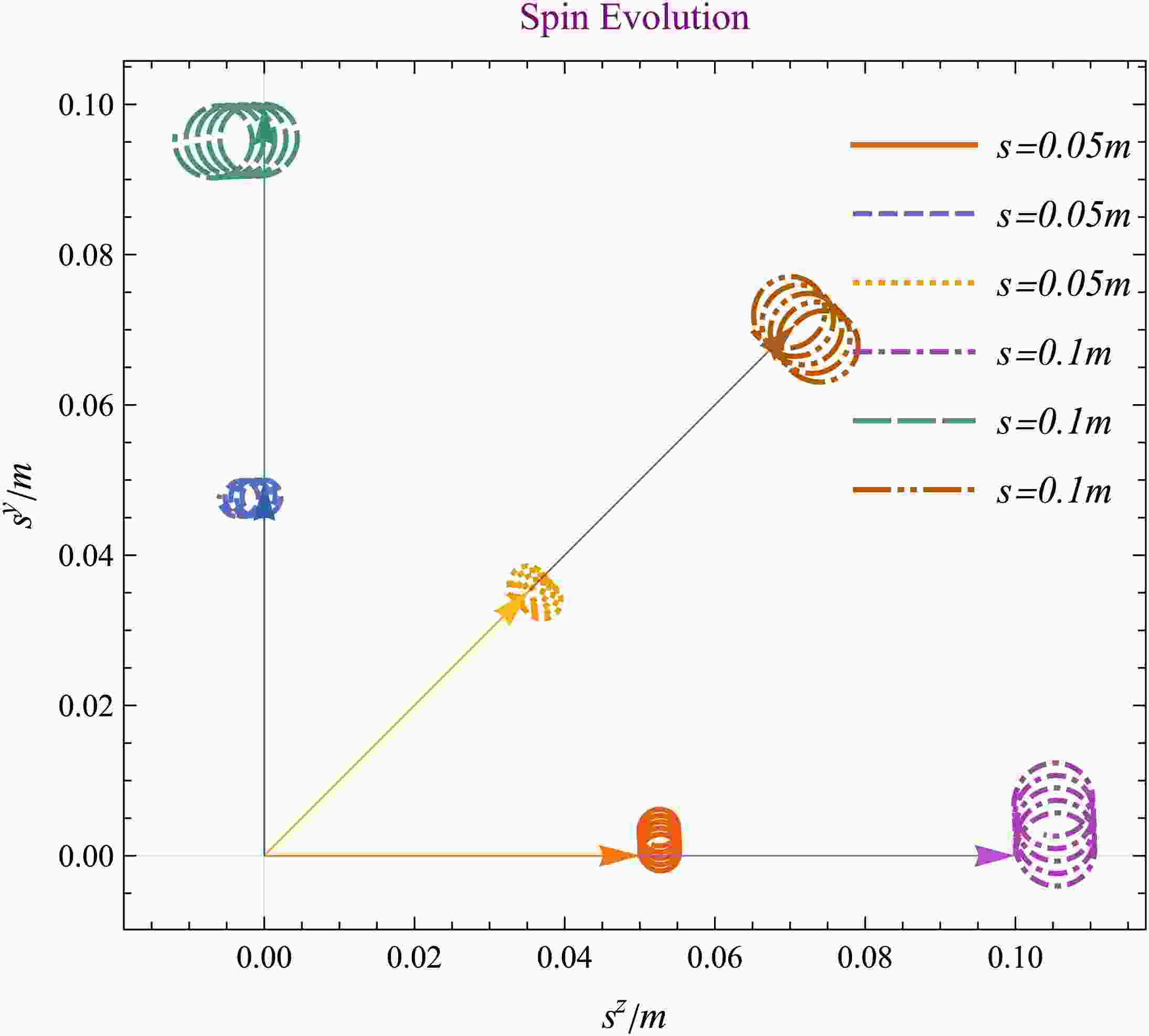
and a particle initially at rest at the origin. Here, h denotes the amplitude of the gravitational wave. We use $h=0.1$ in Fig. 1 to make the behavior visible, and $h= 10^{-10}$ in Fig. 2 to illustrate the weak-field response on magnified axes. Neither value corresponds to a realistic detector strain, and the leading weak-field momentum response scales linearly with h.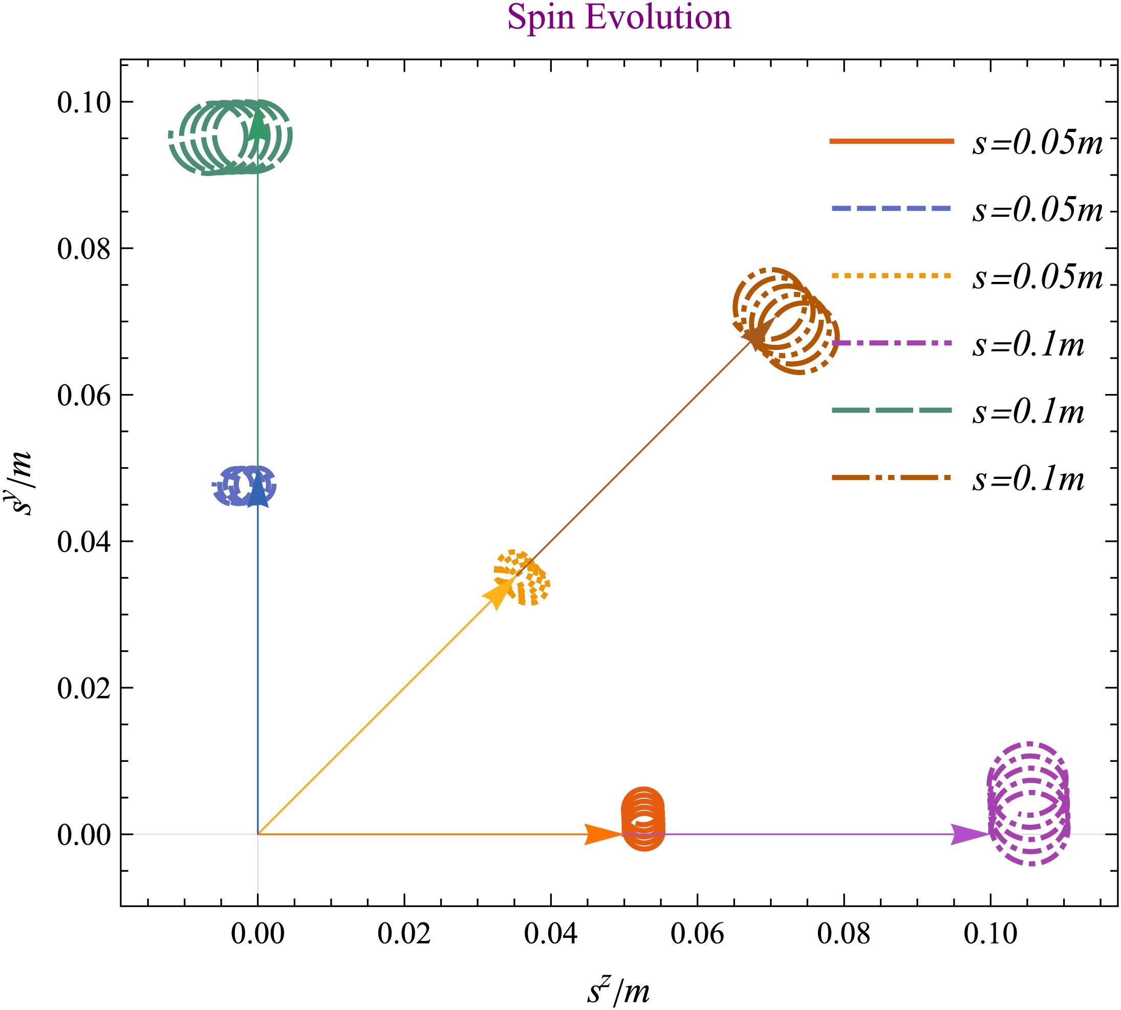

Figure 1.  (color online) Evolution of the coordinate components $s^y(u)$ and $s^z(u)$ for a particle initially at rest, with transverse spin magnitude $s_\perp = 0.1\,m$ and $s_\perp = 0.05\,m$. The gravitational-wave amplitude is $h=10^{-1}$. Although the tetrad components of the spin remain constant, the coordinate components undergo precession driven by the plane-wave geometry; this represents evolution in the coordinate basis rather than a local torque. The value $h=0.1$ is used for visualization and does not represent an astrophysical strain. The arrows indicate the initial spin direction.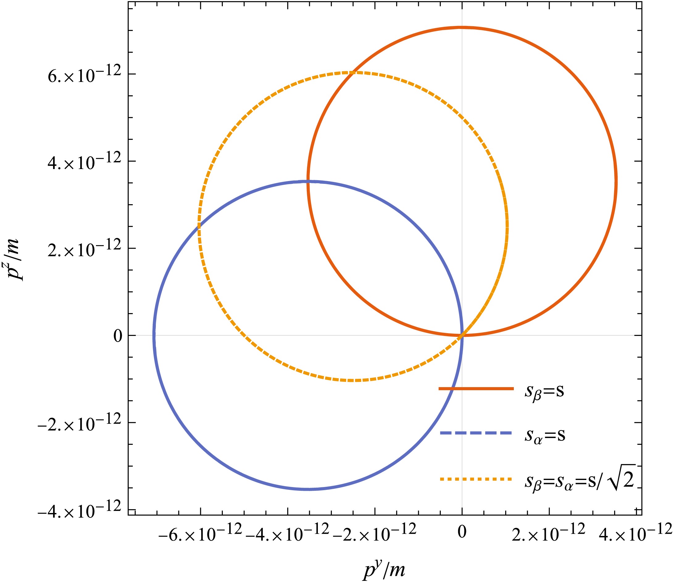

Figure 2.  (color online) Evolution of the transverse momentum components $p^y(u)$ and $p^z(u)$ for a particle initially at rest with transverse spin magnitude $s_\perp=0.1\,m$. The illustrative amplitude is $h=10^{-10}$, and the vertical axes are magnified accordingly. Different colors correspond to different initial orientations in the $(e_2,e_3)$ plane. The oscillatory structure reflects spin–curvature coupling, whereas a geodesic particle would maintain $p^y=p^z=0$. At ${\cal{O}}(hs)$, the curves scale linearly with h; the figure is not intended as a detectability prediction.

For clarity, we decompose the spin into a longitudinal component, $s_\parallel$, aligned with the propagation direction, and a transverse magnitude $s_\perp=\sqrt{s_\alpha^2+s_\beta^2}$.

The nonzero plane-wave tidal curvature has components of the form $R_{uAuB}$, with $A,B\in\{y,z\}$, which explains why the initially static example is sensitive to transverse spin. The tetrad components $(s_\parallel,s_\alpha,s_\beta)$ remain constant, whereas the coordinate components $s^y$ and $s^z$ also reflect the deformation of the Rosen basis. The more direct dynamical quantities are therefore the transverse momentum and displacement relative to the spinless geodesic. For a fixed waveform in the weak-field regime, the retained spin-dependent response is linear in both the wave amplitude h and the spin magnitude s.

Case I: purely longitudinal spin. If the initial spin is aligned with the propagation direction, $s_\perp=0$, then Eqs. (13)–(14) give $J_\alpha=J_\beta=0$. In addition, the terms proportional to $s^u$ in Eqs. (31)–(32) vanish. Thus, all ${\cal{O}}(s)$ corrections to the transverse momentum vanish identically, and the resulting worldline coincides with the geodesic. This confirms that, for the initially static configuration, a purely longitudinal spin does not couple to the plane wave at linear order.

Case II: transverse spin. When the particle carries transverse spin, $s_\perp\neq 0$, the spin–curvature force becomes active and induces oscillatory corrections to the momentum and trajectory. Figure 1 shows the evolution of the coordinate spin components $s^y(u)$ and $s^z(u)$ for particles with two different magnitudes, $s_\perp=0.05\,m$ and $s_\perp=0.1\,m$. Although the tetrad components $(s_\parallel,s_\alpha,s_\beta)$ are constant, the coordinate components exhibit a characteristic precession pattern determined by the rotation angle $\psi(u)$. As the transverse spin increases, the amplitude of the precession ellipse traced in the $(s^y,s^z)$ plane also increases. Since the tetrad components remain constant, this coordinate ellipse reflects the changing Rosen basis rather than a locally measured torque.

Figure 2 shows the corresponding evolution of the momentum components $p^y(u)$ and $p^z(u)$. Whereas the geodesic worldline maintains vanishing transverse momentum, a nonzero transverse spin produces an oscillatory pattern whose phase and amplitude depend on the initial spin orientation (e.g., $s_\alpha=s\,,s_\beta=0$, $s_\beta=s\,,s_\alpha=0$, or $s_\alpha=s_\beta=s/\sqrt{2}$). These three orientations have different projections onto the two polarization axes. These oscillations integrate directly to yield nontrivial transverse motion via Eqs. (41)–(42). Thus, the transverse spin acts as a linear-order source of deviation from geodesic motion.

We additionally test the linear-in-spin solution by integrating the untruncated pole–dipole MPD equations with the TD SSC and the exact TD momentum–velocity relation. The integration evolves the worldline, four-momentum, and all six independent components of the spin tensor, without imposing a linear-in-spin truncation on the numerical equations. We use an adaptive embedded Dormand–Prince 5(4) Runge–Kutta integrator [45] and monitor the mass shell, the TD constraint $S^{\mu\nu}p_\nu=0$, the spin magnitude, and the conserved component $p^u$.

Because $s/m$ alone does not provide a universal estimate of the truncation error for a specified background and initial data, we assess the largest illustrative value directly rather than inferring its accuracy from that ratio. For a deliberately stringent stress test, we use the circularly polarized profile introduced above with $h=0.1$ and evolve an initially static particle for six wave cycles. This amplitude is chosen to magnify nonlinear-in-spin corrections and is not intended to represent an astrophysical gravitational-wave strain. The initial spin is $s_\alpha=s$, $s_\beta=s_\parallel=0$. Defining

we obtain

For the y component, the corresponding differences relative to the peak linear-order signal are $2.11\times10^{-6}$, $5.28\times10^{-5}$, and $2.11\times10^{-4}$; for the z component, they are $1.81\times10^{-6}$, $4.52\times10^{-5}$, and $1.81\times10^{-4}$. The observed scaling is $\max|\Delta p^{y,z}|\propto s^3$ for this particular symmetric initial configuration. This empirical cubic scaling is not assumed in the derivation and should not be interpreted as a general statement about all initial data; rather, it provides a sensitive check of the ${\cal{O}}(s)$ solution in the example considered here. In particular, this test establishes the accuracy of the approximation for this waveform and initial data; it does not replace the inclusion of quadrupole and higher-multipole structure for a specified extended body.

Figure 3 shows the absolute differences $|\Delta p^y|/m$ and $|\Delta p^z|/m$. Over the complete scan, the largest residual among the four monitored constraints and invariants is $4.4\times10^{-14}$. Doubling the output density from 160 to 320 samples per cycle changes $\max|\Delta p^y|/m$ for $s/m=0.1$ by only $2.2\times10^{-9}$ in relative terms. As an additional orientation check, we repeated the six-cycle calculation with $s_\alpha=s_\beta=s/\sqrt{2}$; at $s/m=0.1$, the peak discrepancy relative to the linear $p^y$ signal remains $5.5\times10^{-4}$, while the largest constraint residual is $2.7\times10^{-14}$.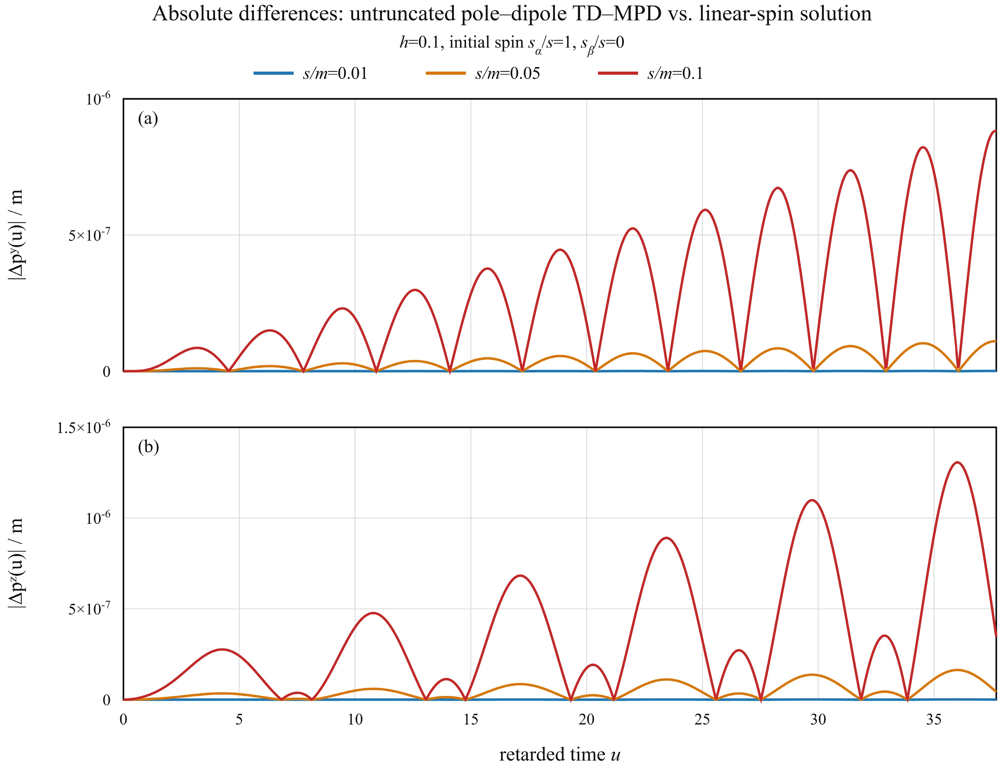

Figure 3.  (color online) Absolute differences between the transverse momenta obtained by integrating the untruncated pole–dipole TD–MPD system and the analytic linear-spin result: (a) $|\Delta p^y|/m$ and (b) $|\Delta p^z|/m$. The particle is initially at rest, with $s_\alpha=s$ and $s_\beta=s_\parallel=0$. The deliberately strong stress-test amplitude is $h=0.1$, and the evolution spans six wave cycles. The small discrepancy and its rapid decrease with $s/m$ validate the linear-spin approximation for this benchmark.

In this work, we have obtained a complete analytic solution for the motion of spinning test particles at linear order in spin in plane gravitational wave backgrounds. By combining a parallel-transported tetrad with the translational Killing symmetries inherent in the geometry, our framework provides an explicit, closed-form decoupling of the linear-spin TD–MPD system for a specific class of exact plane wave spacetimes in Rosen coordinates. Furthermore, because this exact geometric formulation reduces seamlessly to the transverse-traceless (TT) gauge in the weak-field regime ($ |h| \ll 1 $), our analytic integrals can be directly used to compute the leading-order $ {\cal{O}}(h s) $ spin–curvature response of a test body to arbitrary theoretical or numerical waveform templates. This framework therefore provides a highly versatile and mathematically rigorous tool for investigating spin-induced trajectory deviations. The numerical comparison in Sec. V D confirms the accuracy of the linear-spin approximation for the benchmark considered.

Previous work [26, 27] investigated the deviation of precession angles between two freely falling gyroscopes in plane wave spacetimes and established its connection to the velocity memory effect. The present analysis lays the groundwork for extending that study to include spin–curvature coupling. The $ {\cal{O}}(s) $ solution obtained here directly provides the worldline and spin corrections needed to compute the first-order spin-induced modification to the gyroscopic deviation angle. We expect that this coupling will generate additional contributions to gyroscopic memory, especially when the initial spin has transverse components. Whether these contributions are observable requires a specified waveform and observational model and is left for future work.

General exact plane wave spacetimes possess a five-dimensional isometry group [44]. Under the Tulczyjew– Dixon SSC, these five Killing symmetries should, in principle, yield five independent integrals of motion, potentially sufficient to determine the full momentum–spin dynamics without restricting to $ {\cal{O}}(s) $. However, constructing closed-form expressions for these conserved quantities remains challenging. Unlike the Kerr geometry, where the existence of a Killing–Yano tensor leads to a hidden symmetry that decouples the MPD system [14], plane wave isometries form a non-Abelian algebra that does not appear to admit an analogous geometric structure. It is therefore unclear whether a suitable displacement vector or generalized momentum map exists that would allow a similar exact decoupling beyond the linear-spin approximation. The numerical calculation in Sec. V D retains nonlinear spin effects only within the pole–dipole model. A systematic $ {\cal{O}}(s^2) $ expansion would require a new analytic treatment, while a physical extended body may also require quadrupole and higher-multipole information. If other SSCs are considered, such as the Ohashi-Kyrian-Semerák (OKS) condition, the complexity of the MPD equations is significantly reduced. A recent complementary study [46] has shown that, for an arbitrary OKS condition, the dynamics in plane gravitational waves can be determined analytically.

Beyond exact plane waves, it would be natural to investigate spin–curvature coupling in asymptotically flat radiative spacetimes [47, 48]. In that setting, the spin memory effect and gyroscopic memory correspond to asymptotic charges of the extended BMS algebra, and the leading precession induced by gravitational radiation appears at order $ {\cal{O}}(h^{2}) $ [25]. Whether the spin–curvature coupling contributes at order $ {\cal{O}}(hs) $ or $ {\cal{O}}(h^{2}s) $ in this broader framework is an interesting question. Such contributions would represent a new type of spin-sensitive gravitational memory effect that has not yet been systematically explored. Extending the present decoupling to a generic radiative spacetime is nontrivial because the translational Killing vectors used here are generally absent.

Future space-based detectors such as LISA, TianQin, or Taiji [28−31] will monitor test masses in heliocentric or geocentric orbits with unprecedented precision. Although the proof masses are designed to be nearly torque-free, they carry residual angular momentum, and the spacecraft themselves possess controlled attitude dynamics. It is therefore natural to ask whether the spin–curvature coupling derived here could perturb their relative trajectories. For a fixed waveform in the weak-field regime, however, the retained spin-dependent response is linear in both h and s and is expected to be extremely small for realistic strains. Long integration times alone do not establish detectability; a quantitative assessment would require a physical body model, a realistic waveform, a detector observable, and a noise analysis. The analytic MPD solution provides a tractable theoretical input for such future studies rather than a prediction of a detectable signal. It can likewise be used as a local plane-wave or Penrose-limit model for a small compact body, provided that the corresponding multipolar structure is included when required.