A comprehensive cosmographic and thermodynamic analysis of non-metric-matter coupled gravity

Einstein's general theory of relativity (GR) is formulated within the framework of Riemannian geometry, where gravity is interpreted as the manifestation of spacetime curvature. In this theory, the gravitational interaction is described through the geometric properties of a curved spacetime manifold. Observations of Type Ia supernovae provided compelling evidence that the universe is currently undergoing an accelerated phase of expansion [1]. The most widely accepted explanation for this phenomenon is the presence of an exotic energy component, known as dark energy, which dominates the present cosmic energy budget. However, the fundamental nature of dark energy remains unknown, motivating extensive efforts to explore alternative explanations. One of the earliest attempts to account for cosmic acceleration was Einstein's introduction of the cosmological constant, leading to the well-known ΛCDM model. Although this model is remarkably successful in explaining a broad range of cosmological observations, it still suffers from several theoretical challenges [2]. Consequently, considerable attention has been devoted to modifying GR in order to provide a more satisfactory description of the accelerated expansion of the universe and other astrophysical phenomena. Among the proposed modifications, non-Riemannian geometric frameworks have emerged as promising alternatives. Unlike Riemannian geometry, where the metric tensor alone characterizes spacetime, non-Riemannian geometries incorporate additional geometric quantities such as torsion and non-metricity. Torsion originates from tetrad fields and serves as the fundamental geometric quantity in teleparallel gravity, where gravitational effects are entirely encoded in torsion [3]. Alternatively, non-metricity offers a distinct geometric interpretation of gravity and provides novel perspectives on cosmic acceleration without invoking conventional dark energy scenarios. It constitutes the geometric foundation of symmetric teleparallel gravity [4]. The theoretical framework and applications of symmetric teleparallel gravity have been extensively investigated in [5−13]. Furthermore, a comprehensive review of various MGTs and their astrophysical and cosmological implications can be found in [14−24].

A novel class of MGT which is an analogous theory to $ f(R,L_{m}) $ [25] is known as $ f(Q,L_{m}) $ gravity [26] which has been presented in literature by non-minimal couplings in the $ f(Q) $ gravitational framework. In this work, we extend our discussion to another new extension of $ f(Q,L_{m}) $ gravity by considering the inclusion of the scalar term in Lagrangian density of $ f(Q,L_{m}) $ gravity called $ f(Q,L_{m},T) $ theory [27]. This modified version focuses on the complex implications and the growing interest it has received within the scientific community. This gravitational theory provides a non-metricity scalar alternative to a gravity description which does not include curvature and torsion. The addition of the matter sources enable the spacetime geometry to respond to the matter-energy content in the physical system. This property allows $ f(Q,L_{m},T) $ gravity to naturally include matter-geometry interplay and characterizes accelerated cosmic expansion without the need for exotic components. The geometry-matter coupling provides extra effective force which can shed light on the interactions of dark matter and ordinary matter. This theory has highlighted the important implications for gravitational dynamics and has opened new gravitational dynamics and cosmological perspectives. The aim of this theoretical framework is to provide a more complete description of gravity by addressing gaps in existing theories. Thus, the $ f(Q,L_{m},T) $ gravity model offers a straightforward and sound physical basis for studying the non-trivial extensions to Einstein's theory. Furthermore, the interaction between the non-metricity scalar and the matter sources induce a dynamic matter–geometry interaction and greatly enhances our understanding of matter coupling in cosmological systems. The astrophysical implications of $ f(Q,L_{m},T) $ gravity have also been explored through the study of compact stellar objects, revealing that non-Riemannian geometric effects can significantly influence the internal structure and physical characteristics of dense astrophysical systems [28].

The bulk viscosity is a physical important property in cosmic fluid and it appears as natural in many scenarios of early universe, especially for the situation that the non-equilibrium processes associated with accelerating development. The pioneering work of Weinberg [29] showed that bulk viscosity and the temperature dependent relaxation time will be induced naturally in the processes of neutrino decoupling and entropy production, which dominate the dissipation process in primordial plasma. Zimdahl [30] introduced a thermodynamic approach to the study of bulk viscous cosmology and discussed the connections between such models and expansion both at an early and later phases. Furthermore, the electroweak phase transition leads to a sharp change in the equation of state (EoS) and microscopic interaction that generates substantial bulk viscosity [31]. In these periods, the bulk viscosity is no longer neglected and it may produce considerable influences on cosmic dynamics, such as bounce and entropy generation. More recently, bulk viscosity has been investigated as a viable DE model and introduced in various scenarios into violation of ECs such that the late time acceleration is achieved without exotic fields like scalar fields or cosmological constant [32]. Prasad et al. [33] examined a bulk viscous cosmological model that was limited by several data sets and discovered results that were in accordance with recent $ c_{0} $ observations and late-time cosmic acceleration. Pawar and Dabre [34] studied a cosmological model of Bianchi type-V with bulk viscous fluid. Mazumdar et al. [35] established accurate non-singular bounce solutions and discussed about a bulk viscous fluid model. Paul [36] proposed an procedure for the development of bulk viscosity in cosmology to show that simultaneous expansion produces viscous pressure and that viscous cosmology meets the first and second laws of thermodynamics at the apparent horizon.

The concept of bouncing cosmology contradict the accepted theories of singularities associated with the big bang and big crunch theories. Since the overall entropy of an isolated system never decreases according to the second rule of thermodynamics, it is critical to understand how entropy behaves throughout these bounces. The entropy of these models could be affected by the materials used, the physics behind the bounce (like MGTs) or any processes that cause energy to be lost. The evolution of entropy affects the stability of bouncing models. Understanding the role of entropy may also indicate mechanisms to maintain cyclicity, such as entropy reduction or particular interactions in the early universe. If these models can match the behavior of entropy to observations (like large scale structure), then their credibility as alternatives to standard cosmology is enhanced. Furthermore, this analysis can be used to project constraints on any MGTs or quantum corrections to GR that make bounces possible. Bozza and Burni [37] also tackled the problem of anisotropy in bouncing cosmology. Cai et al. [38] used a scalar field to investigate non-singular scenarios. In order to study matter-bounce inflation, Cai [39] developed reconstructed models that provide essential details about the direction of observational cosmology. Ilyas et al. [40] used a number of $ f(R) $ models to examine cosmic dynamics and found that these theories could resolve the underlying singularity. Zubair et al. [41] have studied the viability of the reconstructed cosmological models in the framework of $ f(R,T) $. In [42], the authors considered cosmographic parameters and investigated the evolution of cosmos. The cyclic universe was explored in $ f(R,G) $ gravity models by Lohakare et al. [43]. Their research offers insight into the circumstances that can lead to a bounce and its possible implications for the development of cosmic structures. By parameterizing the Hubble parameter, Singh et al. [44] investigated a bouncing situation in the same theory. In the framework of $ f(Q) $ theory, Dimakis et al. [45] evaluated viable asymmetrical solutions for Kantowski-Sachs and Bianchi type-III spacetime. Their investigation enables it possible to understand the geometric and physical ramifications of anisotropic cosmological models on a more fundamental level. Modified gravity theories have been widely employed to investigate various cosmological phenomena, including bouncing cosmology, dark energy evolution, thermodynamic aspects of the universe, scalar-field dynamics, and the stability of cosmological solutions. The impact of MGTs terms can successfully explain different phases of cosmic evolution while providing viable alternatives to the standard cosmological paradigm [46−51].

The deep and mysterious interplay between gravity and thermodynamics was hinted at early in the work of Hawking with his observation that the temperature at which black holes produce radiation is proportional to their intrinsic gravity, while their entropy is proportional to the area of the horizon [52−54]. This suggests that our understanding of gravitational physics might have its roots in thermodynamics. Jacobson [55] shown that Einstein's formulations can be obtained from basic thermodynamics which highlight the close relationship between spacetime geometry and thermodynamics. These findings have been used to cosmology, particularly in dynamical spacetime where apparent boundaries are connected in temperature and entropy. The main goal of this paper is to study the effect of the bulk viscosity on cosmic pressure and its consequence for the dynamical evolution of the universe in cosmological bouncing model. The manuscript is organized as follows. In Section II, we discuss the introductory background of $ f(Q,L_{m},T) $ gravity and then derive field equations for this model in presence of bulk viscous fluid. We investigate the possibility of non-singular bounce by analyzing the evolution of several important cosmological parameters in Section III. Moreover, we discuss the physical aspects of the model by examining stability through adiabatic speed of sound and cosmographic diagnostics in Section IV. Section V presents the validity of this theoretical approach through second law of thermodynamics. Finally, Section VI conclude with a summary of our main results and their cosmological implications.

In this section, we outline the fundamentals of modified $ f(Q,L_{m},T) $ gravity and derive the corresponding field equations. The expression for a general affine connection is given by [56]

where $ \Gamma^{\varphi}_{\; \gamma\nu} $ indicates the Christoffel symbols, $ \mathrm{C}^{\varphi}_{\; \gamma\nu} $ is the the contortion tensor and $ L^{\varphi}_{\; \gamma\nu} $ is the disformation tensor. The torsion tensor is used to express the contortion tensor as follows

The disformation tensor is derived from non-metricity as

where the definition of the non-metricity tensor is as follows

Since the non-metricity tensor possesses three indices, two independent traces can be constructed by contracting different pairs of indices. These traces are defined as

Here, $ Q_{\varphi} $ and $ \bar{Q}_{\varphi} $ denote the two independent traces of the non-metricity tensor, obtained by contracting different pairs of indices. In general, these quantities are distinct and both contribute to the construction of the superpotential tensor and the non-metricity scalar. Both traces play an essential role in constructing the superpotential tensor and the non-metricity scalar, which are fundamental ingredients of the symmetric teleparallel formulation of gravity.

The non-metricity scalar is given by

The detailed calculation of the non-metricity scalar is provided in [57]. The superpotential function is defined as

Using the superpotential, the non-metricity scalar can be obtained as

The gravitational action in the context of $ f(Q,L_{m},T) $ gravity is given by

Here, g denotes the determinant of the metric tensor and $ \kappa=1 $ is the coupling constant. By varying the action in Eq. (9), we obtain the field equations as

The detailed derivation of the variation of the non-metricity scalar is presented in [57]. Where the energy-momentum tensor (EMT) is given by $ T_{\varphi\gamma}= -\dfrac{2}{\sqrt{-g}}\dfrac{\delta(\sqrt{-g}L_{m})}{\delta g^{\varphi\gamma}} $ with the trace $ T=g^{\varphi\gamma}T_{\varphi\gamma} $ and the tensor $ \Theta=g^{\nu \varsigma}\dfrac{\delta T_{\nu\varsigma}}{\delta g^{\varphi\gamma}} $. We examine a Friedmann-Robertson-Walker (FRW) cosmic model characterized by the scale factor as

This homogeneous and isotropic model of the universe provides insight into the behavior of the cosmos and provides essential cosmic basis to analyze cosmological dynamics. We consider the isotropic matter configuration as

In this case, $ \tilde{p}=p-3\varepsilon H $ denotes the fluid's effective pressure. The field equations that are generated by applying Eqs. (10)−(12) are given as

where $ Q=6H^{2} $, $ H=\dot a/a $ is the Hubble parameter and dot denotes differentiation with respect to time. Here, $ f_Q=\dfrac{\partial f}{\partial Q} $, $ f_{T}=\dfrac{\partial f}{\partial T} $ and $ f_{L_m} = \dfrac{\partial f}{\partial L_m} $. The existence of numerous functions and their higher-order derivatives complicates the field equations, making it difficult to obtain exact cosmological solutions. We intend to concentrate on a particular form to address the situation and identify physically significant alternatives. This has the advantage of preserving the primary characteristics of the matter-geometry interaction while facilitating simplified access to cosmic dynamics. Therefore, our choice of this form provides an appropriate setting for investigating the growth of the universe and the necessary conditions for a non-singular bounce

Here, $ \sigma_{1} $ and $ \sigma_{2} $ are arbitrary non-zero constants. The choice of the matter-Lagrangian significantly affects the dynamics of a non-singular cosmic model. During the dynamics of source matter in the accelerated cosmos, $ (L_{m}=\tilde{p}) $ is assumed as the form of the Lagrangian density for isotropic and homogeneous fluid distributions. This is commonly used in literature [53, 54] because it leads to the standard EMT for a perfect fluid. Using Eqs. (13)–(15), we obtain

The effective pressure contains the bulk viscous correction with bulk-viscosity coefficient is defined by ε. This correction is important because it can generate an effective negative pressure, which helps to support accelerated expansion and ECs violation near the bounce. In the context of cosmology, bulk viscosity arises when the expanding universe deviates from thermodynamic equilibrium. Such deviations induce dissipative effects that can change the behavior of the universe during different epochs such as inflation, radiation-dominant and late-time accelerated expansion. The bulk viscous coefficient is considered as [35]

Here, $ t, \tau_{0}, m $ are constant parameters. Among various dissipative mechanisms, bulk viscosity provides an effective macroscopic description of entropy production and internal friction arising from particle interactions, phase transitions, and deviations from local thermodynamic equilibrium. In bouncing cosmology, viscous effects can smooth the evolution near the bounce, suppress potential instabilities, and contribute to a regular transition between the contracting and expanding phases. Motivated by these physical considerations, we incorporate bulk viscosity into the cosmic fluid through an effective pressure term. Furthermore, in the framework of $ f(Q,L_m,T) $ gravity, matter-geometry interactions can naturally induce effective dissipative phenomena. This choice allows us to investigate how dissipation influences the background dynamics and stability of bouncing solutions in $ f(Q,L_m,T) $ gravity. The effective pressure becomes

By varying the Eq. (13), the modified Friedmann equation associated to the model Eq. (15) is obtained as

where

We use a barotropic equation of the fluid, which expresses pressure as a function of energy density. This assumption simplifies the dynamical system, resulting in an instantaneous form of cosmic evolution with only one parameter. It also offers a physically meaningful scheme for studying cosmic fluids and allows one to check the bouncing regime as well as stability conditions. The corresponding equation is defined as

By using Eqs. (19)−(21), we obtain

In such a scenario, the above equation is computed for an exact expression of energy density based on cosmic time and model parameters as

We use a modified conservation equation to calculate energy density by considering matter-geometry coupling and viscous effects. The proposed formulation provides a consistent description of energy interchange in modified gravity and is useful for studying cosmic processes

Using Eqs. (19) and (23) into Eq. (24), we get the expression for Hubble parameter as

Here, $ c_{0} $ is an intigration constant. To ensure a non-singular cosmological bounce, we reconstruct the scale factor by integrating the relation $ H=\dot a/a $. The scale factor that represents the smooth transition from a contracting to an expanding phase is formulated from the Hubble relation as

The resulting equation is finite and non-zero throughout cosmic time, indicating no physical singularities. Now, we derive the effective viscous pressure as

The viscous contribution in Eq. (27) demonstrates the interplay between barotropic pressure and dissipative bulk viscous effects which provides a generalized description of the cosmic fluid in non-equilibrium thermodynamics. The expression of pressure term plays a crucial role in determining the expansion history and offer a viable mechanism for explaining late time acceleration in this MGT.

In this section, we outline the fundamentals of modified $ f(Q,L_{m},T) $ gravity and derive the corresponding field equations. The expression for a general affine connection is given by [56]

where $ \Gamma^{\varphi}_{\; \gamma\nu} $ indicates the Christoffel symbols, $ \mathrm{C}^{\varphi}_{\; \gamma\nu} $ is the the contortion tensor and $ L^{\varphi}_{\; \gamma\nu} $ is the disformation tensor. The torsion tensor is used to express the contortion tensor as follows

The disformation tensor is derived from non-metricity as

where the definition of the non-metricity tensor is as follows

Since the non-metricity tensor possesses three indices, two independent traces can be constructed by contracting different pairs of indices. These traces are defined as

Here, $ Q_{\varphi} $ and $ \bar{Q}_{\varphi} $ denote the two independent traces of the non-metricity tensor, obtained by contracting different pairs of indices. In general, these quantities are distinct and both contribute to the construction of the superpotential tensor and the non-metricity scalar. Both traces play an essential role in constructing the superpotential tensor and the non-metricity scalar, which are fundamental ingredients of the symmetric teleparallel formulation of gravity.

The non-metricity scalar is given by

The detailed calculation of the non-metricity scalar is provided in [57]. The superpotential function is defined as

Using the superpotential, the non-metricity scalar can be obtained as

The gravitational action in the context of $ f(Q,L_{m},T) $ gravity is given by

Here, g denotes the determinant of the metric tensor and $ \kappa=1 $ is the coupling constant. By varying the action in Eq. (9), we obtain the field equations as

The detailed derivation of the variation of the non-metricity scalar is presented in [57]. Where the energy-momentum tensor (EMT) is given by $ T_{\varphi\gamma}= -\dfrac{2}{\sqrt{-g}}\dfrac{\delta(\sqrt{-g}L_{m})}{\delta g^{\varphi\gamma}} $ with the trace $ T=g^{\varphi\gamma}T_{\varphi\gamma} $ and the tensor $ \Theta=g^{\nu \varsigma}\dfrac{\delta T_{\nu\varsigma}}{\delta g^{\varphi\gamma}} $. We examine a Friedmann-Robertson-Walker (FRW) cosmic model characterized by the scale factor as

This homogeneous and isotropic model of the universe provides insight into the behavior of the cosmos and provides essential cosmic basis to analyze cosmological dynamics. We consider the isotropic matter configuration as

In this case, $ \tilde{p}=p-3\varepsilon H $ denotes the fluid's effective pressure. The field equations that are generated by applying Eqs. (10)−(12) are given as

where $ Q=6H^{2} $, $ H=\dot a/a $ is the Hubble parameter and dot denotes differentiation with respect to time. Here, $ f_Q=\dfrac{\partial f}{\partial Q} $, $ f_{T}=\dfrac{\partial f}{\partial T} $ and $ f_{L_m} = \dfrac{\partial f}{\partial L_m} $. The existence of numerous functions and their higher-order derivatives complicates the field equations, making it difficult to obtain exact cosmological solutions. We intend to concentrate on a particular form to address the situation and identify physically significant alternatives. This has the advantage of preserving the primary characteristics of the matter-geometry interaction while facilitating simplified access to cosmic dynamics. Therefore, our choice of this form provides an appropriate setting for investigating the growth of the universe and the necessary conditions for a non-singular bounce

Here, $ \sigma_{1} $ and $ \sigma_{2} $ are arbitrary non-zero constants. The choice of the matter-Lagrangian significantly affects the dynamics of a non-singular cosmic model. During the dynamics of source matter in the accelerated cosmos, $ (L_{m}=\tilde{p}) $ is assumed as the form of the Lagrangian density for isotropic and homogeneous fluid distributions. This is commonly used in literature [53, 54] because it leads to the standard EMT for a perfect fluid. Using Eqs. (13)–(15), we obtain

The effective pressure contains the bulk viscous correction with bulk-viscosity coefficient is defined by ε. This correction is important because it can generate an effective negative pressure, which helps to support accelerated expansion and ECs violation near the bounce. In the context of cosmology, bulk viscosity arises when the expanding universe deviates from thermodynamic equilibrium. Such deviations induce dissipative effects that can change the behavior of the universe during different epochs such as inflation, radiation-dominant and late-time accelerated expansion. The bulk viscous coefficient is considered as [35]

Here, $ t, \tau_{0}, m $ are constant parameters. Among various dissipative mechanisms, bulk viscosity provides an effective macroscopic description of entropy production and internal friction arising from particle interactions, phase transitions, and deviations from local thermodynamic equilibrium. In bouncing cosmology, viscous effects can smooth the evolution near the bounce, suppress potential instabilities, and contribute to a regular transition between the contracting and expanding phases. Motivated by these physical considerations, we incorporate bulk viscosity into the cosmic fluid through an effective pressure term. Furthermore, in the framework of $ f(Q,L_m,T) $ gravity, matter-geometry interactions can naturally induce effective dissipative phenomena. This choice allows us to investigate how dissipation influences the background dynamics and stability of bouncing solutions in $ f(Q,L_m,T) $ gravity. The effective pressure becomes

By varying the Eq. (13), the modified Friedmann equation associated to the model Eq. (15) is obtained as

where

We use a barotropic equation of the fluid, which expresses pressure as a function of energy density. This assumption simplifies the dynamical system, resulting in an instantaneous form of cosmic evolution with only one parameter. It also offers a physically meaningful scheme for studying cosmic fluids and allows one to check the bouncing regime as well as stability conditions. The corresponding equation is defined as

By using Eqs. (19)−(21), we obtain

In such a scenario, the above equation is computed for an exact expression of energy density based on cosmic time and model parameters as

We use a modified conservation equation to calculate energy density by considering matter-geometry coupling and viscous effects. The proposed formulation provides a consistent description of energy interchange in modified gravity and is useful for studying cosmic processes

Using Eqs. (19) and (23) into Eq. (24), we get the expression for Hubble parameter as

Here, $ c_{0} $ is an intigration constant. To ensure a non-singular cosmological bounce, we reconstruct the scale factor by integrating the relation $ H=\dot a/a $. The scale factor that represents the smooth transition from a contracting to an expanding phase is formulated from the Hubble relation as

The resulting equation is finite and non-zero throughout cosmic time, indicating no physical singularities. Now, we derive the effective viscous pressure as

The viscous contribution in Eq. (27) demonstrates the interplay between barotropic pressure and dissipative bulk viscous effects which provides a generalized description of the cosmic fluid in non-equilibrium thermodynamics. The expression of pressure term plays a crucial role in determining the expansion history and offer a viable mechanism for explaining late time acceleration in this MGT.

In the framework of bouncing cosmology, the evolution of cosmos is described by a smooth crossover from an early contracting era to an expanding phase without a singularity. This happens when the cosmic evolution is effectively used in a scenario in which all geometrical and physical quantities remain finite. The action of the universe can be characterized by cosmological parameters, notably the Hubble parameter and its derivatives. Therefore, under the appropriate scenarios, a non-singular bounce could occur because the Hubble parameter regulates the cosmic phases of expansion and contraction. The universe smoothly bounces off after attaining a minimal non-zero value for the scale factor at the bounce, never reaching infinite density or pressure. Thus, bouncing cosmology is a powerful tool for testing alternative gravity theories as it challenges the underlying theory and cosmic effective matter composition. In contrast, in the standard cosmological framework where a primordial singularity is accommodated, bouncing cosmology indicates the acceptance of a smooth transition from a contracting to an expanding region. This model not only corrects the interplay of cosmic origin but also provides new phenomena in connection with the early-cosmic dynamics. To consider more realistic successful bouncing solutions, in the subsequent subsections, we analyze the dynamical evolution of different cosmic parameters. These parameters are important quantities for the evaluation of the compatibility of the cosmic bounce and also as observational tests to discriminate them from an inflationary scenario. In this theory, the requirements for a successful cosmological bounce in a flat FRW background are expressed as

● The size of the universe as a function of time is represented by the scale factor. To prevent the cosmic singularity, it tends to shrink during a contraction phase and reach a finite non-zero minimum value before expansion. The scale factor has a non-vanishing minimum value at the bouncing epoch.

● The expansion and contraction of the cosmos is controlled by the Hubble parameter. In the case of bouncing, it approaches smoothly negative values in the contracting phase and positive ones in the expanding phase, which guarantees the regular cosmic change. The expansion rate is temporarily zero at the bounce point because the Hubble parameter disappears at bounce.

● The time derivative of the Hubble parameter determines the nature of cosmic evolution. A positive bounce characteristics stabilize the dynamical system and ensures a smooth transition from the accelerated phase to the decelerated phase.

● The matter components are essential in governing cosmic dynamics. In the MGT, effective matter supports the non-singular bouncing solutions together with the geometrical corrections. Near the bounce, negative pressure arises which helps the universe transition from contraction to expansion. After the bounce, the matter density decreases positively as the universe expands.

● For a viable bouncing model, the deceleration parameter deviates to be negative, the cosmos accelerates. On the other hand, when the deceleration parameter leans towards positive, the universe expands.

In the framework of bouncing cosmology, the evolution of cosmos is described by a smooth crossover from an early contracting era to an expanding phase without a singularity. This happens when the cosmic evolution is effectively used in a scenario in which all geometrical and physical quantities remain finite. The action of the universe can be characterized by cosmological parameters, notably the Hubble parameter and its derivatives. Therefore, under the appropriate scenarios, a non-singular bounce could occur because the Hubble parameter regulates the cosmic phases of expansion and contraction. The universe smoothly bounces off after attaining a minimal non-zero value for the scale factor at the bounce, never reaching infinite density or pressure. Thus, bouncing cosmology is a powerful tool for testing alternative gravity theories as it challenges the underlying theory and cosmic effective matter composition. In contrast, in the standard cosmological framework where a primordial singularity is accommodated, bouncing cosmology indicates the acceptance of a smooth transition from a contracting to an expanding region. This model not only corrects the interplay of cosmic origin but also provides new phenomena in connection with the early-cosmic dynamics. To consider more realistic successful bouncing solutions, in the subsequent subsections, we analyze the dynamical evolution of different cosmic parameters. These parameters are important quantities for the evaluation of the compatibility of the cosmic bounce and also as observational tests to discriminate them from an inflationary scenario. In this theory, the requirements for a successful cosmological bounce in a flat FRW background are expressed as

● The size of the universe as a function of time is represented by the scale factor. To prevent the cosmic singularity, it tends to shrink during a contraction phase and reach a finite non-zero minimum value before expansion. The scale factor has a non-vanishing minimum value at the bouncing epoch.

● The expansion and contraction of the cosmos is controlled by the Hubble parameter. In the case of bouncing, it approaches smoothly negative values in the contracting phase and positive ones in the expanding phase, which guarantees the regular cosmic change. The expansion rate is temporarily zero at the bounce point because the Hubble parameter disappears at bounce.

● The time derivative of the Hubble parameter determines the nature of cosmic evolution. A positive bounce characteristics stabilize the dynamical system and ensures a smooth transition from the accelerated phase to the decelerated phase.

● The matter components are essential in governing cosmic dynamics. In the MGT, effective matter supports the non-singular bouncing solutions together with the geometrical corrections. Near the bounce, negative pressure arises which helps the universe transition from contraction to expansion. After the bounce, the matter density decreases positively as the universe expands.

● For a viable bouncing model, the deceleration parameter deviates to be negative, the cosmos accelerates. On the other hand, when the deceleration parameter leans towards positive, the universe expands.

The Hubble parameter is an essential cosmic parameter to understand the cosmic bounce as it defines the cosmic expansion and contraction. A positive Hubble parameter indicates universe expansion, while negative values indicate contraction. The interaction of expansion and contraction is indicated by the Hubble parameter being zero at the bouncing epoch. A physically realistic bounce requires that the Hubble parameter should be greater than zero following the bounce regime and smaller than zero prior to the bounce. The behavior of the time derivative of the Hubble parameter is essential as it provides insight into the bounce mechanism. 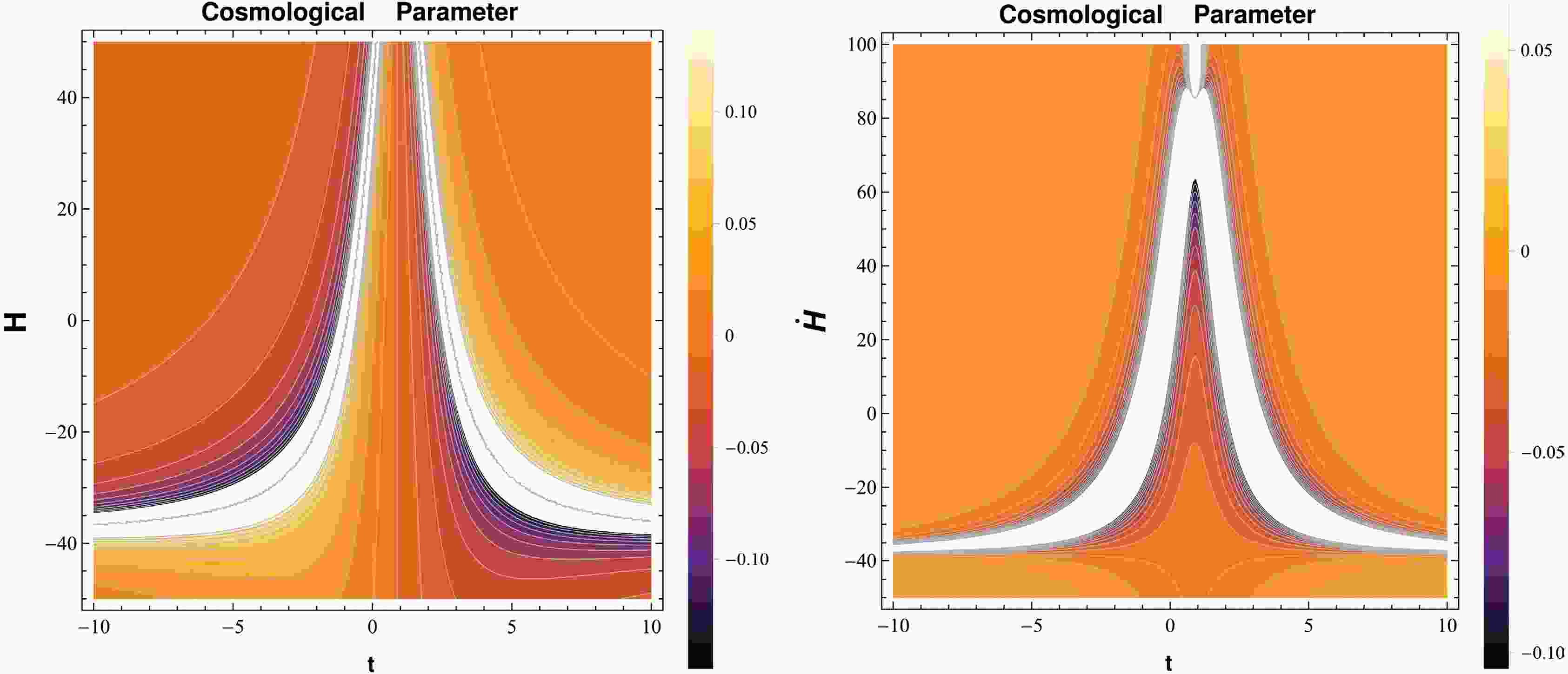The positive value of $ \dot{H} $ around the bouncing epoch indicates that the cosmos is transitioning from decelerating contraction to accelerating expansion, a necessary requirement for bounce. The color bars represent the magnitude variation of the plotted cosmological quantities as a function of time. Specifically, the color gradient indicates the evolution intensity of the corresponding physical quantity, where different colors correspond to different numerical ranges, allowing a clear visualization of dynamical transitions around the bouncing epoch. This is demonstrated by their gradients, which show how the associated parametric absolute value changes with time, making the transition around the bounce more noticeable and physically interpretable. Figure 1 depicts the evolution of Hubble parameter and its derivative over time. The left panel of Fig. 1 indicates symmetry with respect to $ t=0 $, which is consistent with other classical solutions. This is a key feature of non-singular bouncing cosmology. For $ t<0 $, the Hubble parameter takes negative values, indicating a contracting universe. As time approaches the bounce point, H smoothly increases and reaches zero at $ t=0 $, marking the transition from contraction to expansion. For $ t>0 $, H becomes positive, which signifies an expanding universe. This continuous and finite behavior confirms the absence of singularities and supports a regular cosmic evolution. The right panel of Fig. 1 shows the behavior of the temporal derivative, which exhibits non-singular behavior near the bounce, a necessary physical criterion for bouncing models. The positive value of $ (\dot{H}) $ indicates that the cosmos is transitioning from a contraction to an expansion phase. The model reverts to a quasi-standard expansion as it moves away from the bounce. In contrast, the standard ΛCDM model predicts a big bang with diminishing H and accelerated expansion due to DE, rather than a contraction and expansion cycle. The suggested model replaces the ΛCDM initial singularity with a limited, smooth transition, offering a new explanation for early cosmic history and late-time expansion.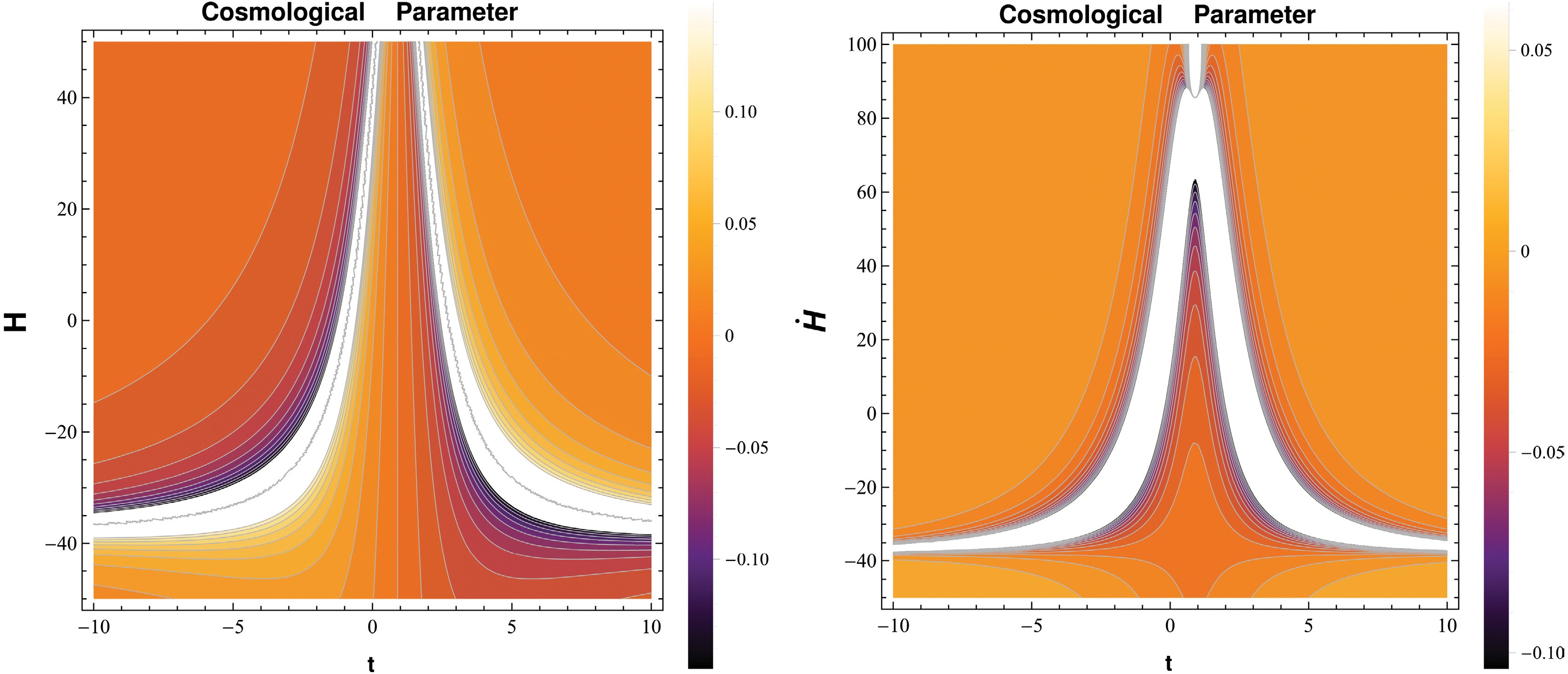

Figure 1.  (color online) Evolution of Hubble parameter (left plot) and temporal derivative (right plot) against time.

The Hubble parameter is an essential cosmic parameter to understand the cosmic bounce as it defines the cosmic expansion and contraction. A positive Hubble parameter indicates universe expansion, while negative values indicate contraction. The interaction of expansion and contraction is indicated by the Hubble parameter being zero at the bouncing epoch. A physically realistic bounce requires that the Hubble parameter should be greater than zero following the bounce regime and smaller than zero prior to the bounce. The behavior of the time derivative of the Hubble parameter is essential as it provides insight into the bounce mechanism. The positive value of $ \dot{H} $ around the bouncing epoch indicates that the cosmos is transitioning from decelerating contraction to accelerating expansion, a necessary requirement for bounce. The color bars represent the magnitude variation of the plotted cosmological quantities as a function of time. Specifically, the color gradient indicates the evolution intensity of the corresponding physical quantity, where different colors correspond to different numerical ranges, allowing a clear visualization of dynamical transitions around the bouncing epoch. This is demonstrated by their gradients, which show how the associated parametric absolute value changes with time, making the transition around the bounce more noticeable and physically interpretable. Figure 1 depicts the evolution of Hubble parameter and its derivative over time. The left panel of Fig. 1 indicates symmetry with respect to $ t=0 $, which is consistent with other classical solutions. This is a key feature of non-singular bouncing cosmology. For $ t<0 $, the Hubble parameter takes negative values, indicating a contracting universe. As time approaches the bounce point, H smoothly increases and reaches zero at $ t=0 $, marking the transition from contraction to expansion. For $ t>0 $, H becomes positive, which signifies an expanding universe. This continuous and finite behavior confirms the absence of singularities and supports a regular cosmic evolution. The right panel of Fig. 1 shows the behavior of the temporal derivative, which exhibits non-singular behavior near the bounce, a necessary physical criterion for bouncing models. The positive value of $ (\dot{H}) $ indicates that the cosmos is transitioning from a contraction to an expansion phase. The model reverts to a quasi-standard expansion as it moves away from the bounce. In contrast, the standard ΛCDM model predicts a big bang with diminishing H and accelerated expansion due to DE, rather than a contraction and expansion cycle. The suggested model replaces the ΛCDM initial singularity with a limited, smooth transition, offering a new explanation for early cosmic history and late-time expansion.

Figure 1.  (color online) Evolution of Hubble parameter (left plot) and temporal derivative (right plot) against time.

The scale factor is crucial to define the development of the universe. It determines how much the cosmos expands or contracts relative to itself. It is a time-dependent positive function that quantifies how the distances between comoving points evolve with time. Figure 2 depicts the behavior of the scale factor as a function, which clearly shows the dynamical transition from contraction to bounce and expansion. The plot indicates that the scale factor is positive for any values in its domain and implies that there is no cosmological singularity. For negative time $ (t \lt 0) $, the plot bends towards lower $ a(t) $ values, signaling a smoothly contracting phase where the universe is slowly collapsing. It does not vanish, which indicates that the cosmos does not have a big bang-like singularity and shows the bouncing phase is consistent. Following the bounce $ (t>0) $, the plot shows the expansion and move toward larger $ a(t) $ corresponding to monotonically expanding dynamics. The pattern of the graph at $ t=0 $ indicates a time-reversal symmetric bounce with the pre-bounce contraction reflected in the post-bounce expansion. The graph's smooth gradients indicate a constant expansion rate, resulting in finite Hubble and curvature scalars. This behavior differs from the Newtonian ΛCDM scenario, which involves an initial singularity with a scale factor of zero and monotonic expansion throughout. The bouncing paradigm uses a non-zero minimum of $ a(t) $ to describe finite energy densities and curvatures at all times. This provides a better description of early universe dynamics and an alternative approach to the problem of cosmological singularity, which is also compatible with late time cosmic accelerated expansion.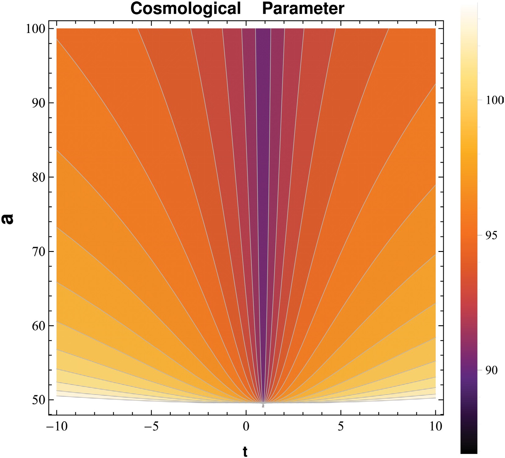

Figure 2.  (color online) Graph of the scale factor corresponding to time.

The scale factor is crucial to define the development of the universe. It determines how much the cosmos expands or contracts relative to itself. It is a time-dependent positive function that quantifies how the distances between comoving points evolve with time. Figure 2 depicts the behavior of the scale factor as a function, which clearly shows the dynamical transition from contraction to bounce and expansion. The plot indicates that the scale factor is positive for any values in its domain and implies that there is no cosmological singularity. For negative time $ (t \lt 0) $, the plot bends towards lower $ a(t) $ values, signaling a smoothly contracting phase where the universe is slowly collapsing. It does not vanish, which indicates that the cosmos does not have a big bang-like singularity and shows the bouncing phase is consistent. Following the bounce $ (t>0) $, the plot shows the expansion and move toward larger $ a(t) $ corresponding to monotonically expanding dynamics. The pattern of the graph at $ t=0 $ indicates a time-reversal symmetric bounce with the pre-bounce contraction reflected in the post-bounce expansion. The graph's smooth gradients indicate a constant expansion rate, resulting in finite Hubble and curvature scalars. This behavior differs from the Newtonian ΛCDM scenario, which involves an initial singularity with a scale factor of zero and monotonic expansion throughout. The bouncing paradigm uses a non-zero minimum of $ a(t) $ to describe finite energy densities and curvatures at all times. This provides a better description of early universe dynamics and an alternative approach to the problem of cosmological singularity, which is also compatible with late time cosmic accelerated expansion.

Figure 2.  (color online) Graph of the scale factor corresponding to time.

This parameter measures the rate at which the universe is expanding, such as a positive trend denotes an accelerated cosmos, while a negative profile denotes an accelerating universe. The value of the deceleration parameter is written as

The plot of the deceleration parameter clearly determines the dynamical transition associated with a non-singular bouncing cosmology in Fig. 3. Near the bounce epoch $ t=0 $, the deceleration parameter exhibits a divergence toward large negative values, which indicate a strong accelerated phase that is necessary to halt the contracting universe and trigger the bounce. This pronounced negative region reflects the dominance of repulsive effects arising from viscous contributions and MGT terms. As time moves away from the bounce on either side of bouncing point, the magnitude of q gradually decreases and approaches smaller values that signifies a smooth transition from extreme acceleration to a less accelerated and decelerated regime. The symmetry of the plot about $ t=0 $ confirms the time-symmetric nature of the bounce, while the continuous gradient in color demonstrates that the transition is smooth rather than abrupt, reinforcing the non-singular and physically viable behavior of the cosmological model.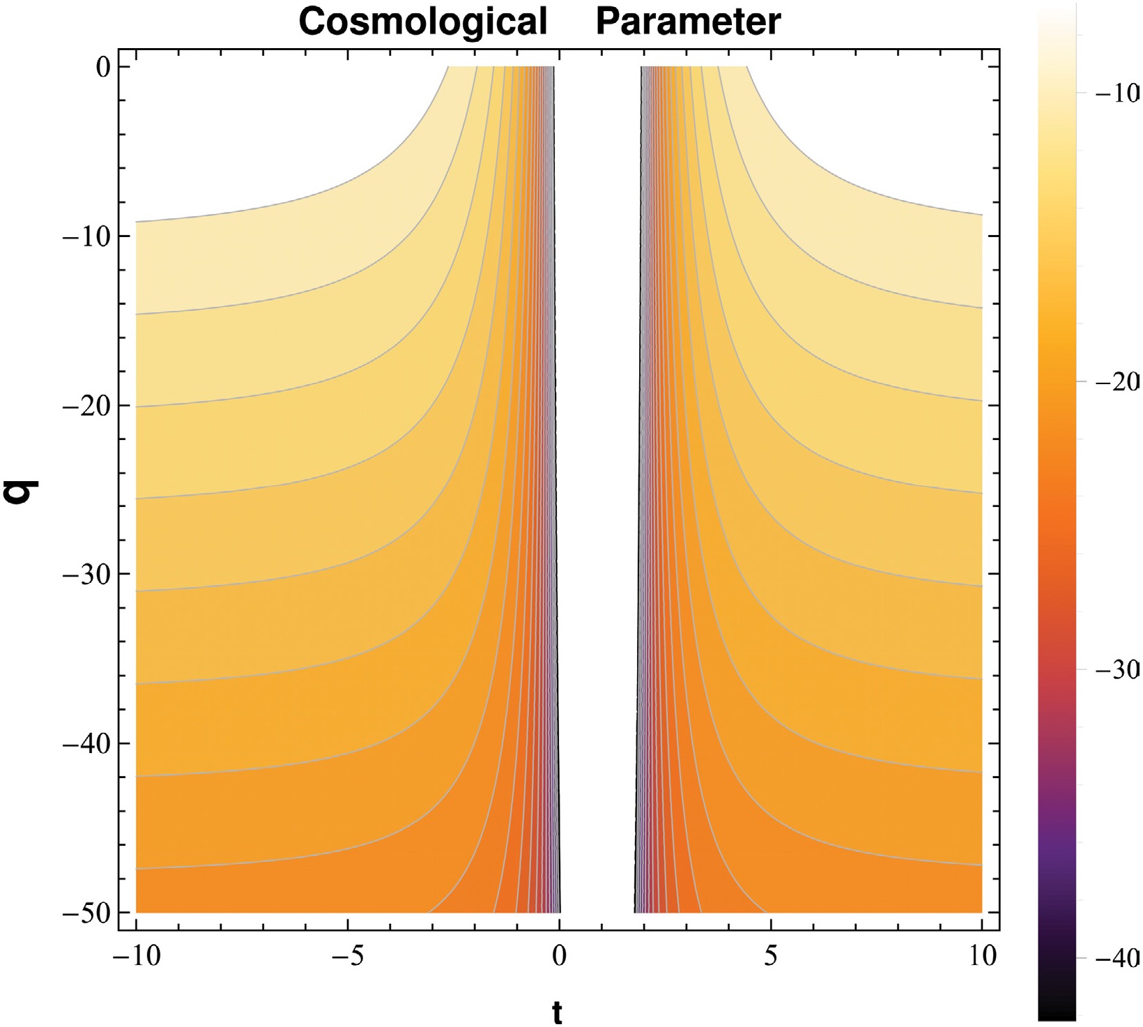

Figure 3.  (color online) Plot of the deceleration parameter against time.

This parameter measures the rate at which the universe is expanding, such as a positive trend denotes an accelerated cosmos, while a negative profile denotes an accelerating universe. The value of the deceleration parameter is written as

The plot of the deceleration parameter clearly determines the dynamical transition associated with a non-singular bouncing cosmology in Fig. 3. Near the bounce epoch $ t=0 $, the deceleration parameter exhibits a divergence toward large negative values, which indicate a strong accelerated phase that is necessary to halt the contracting universe and trigger the bounce. This pronounced negative region reflects the dominance of repulsive effects arising from viscous contributions and MGT terms. As time moves away from the bounce on either side of bouncing point, the magnitude of q gradually decreases and approaches smaller values that signifies a smooth transition from extreme acceleration to a less accelerated and decelerated regime. The symmetry of the plot about $ t=0 $ confirms the time-symmetric nature of the bounce, while the continuous gradient in color demonstrates that the transition is smooth rather than abrupt, reinforcing the non-singular and physically viable behavior of the cosmological model.

Figure 3.  (color online) Plot of the deceleration parameter against time.

In the present section, we examine how cosmic geometry is influenced by matter variables. Incorporating additional terms may yield significant outcomes. The examined bulk viscosity model offers a brief method for examining how various cosmic processes are affected by matter characteristics. Using Eq. (25) into Eqs. (23) and (27), we get the explicit expression of energy density and pressure

The dynamic evolution of energy density and pressure over time is shown in Fig. 4. This behavior depicts the evolution of the matter components corresponding to time. The energy density is symmetric about the bounce point and is positive throughout cosmic history. A large value of time leads to a higher energy density, suggesting that a stronger coupling encourages an immediate increase in energy density. Conversely, the pressure is negative and exhibits a bell-shaped behavior with a distinct minimum value at bounce, early and late times. Larger values of the parameter enhance the magnitude of this negative pressure and emphasize its indispensable part in cosmological dynamics. The presence of positive energy density coupled with a negative pressure results in the effective characteristics of exotic energy that exerts a repulsive force on a large scale. Consequently, these components are used to successfully realize scenarios for non-singular bouncing cosmology. The evolution of the matter variables is examined to verify the physical regularity of the cosmological solution. The finiteness of the energy density and pressure throughout cosmic evolution directly reflects the non-singular behavior of the scale factor and metric functions. This analysis is crucial, as a non-singular metric alone is not sufficient, a viable bouncing model must also ensure that all physical matter quantities remain bounded and well-defined across the bounce.

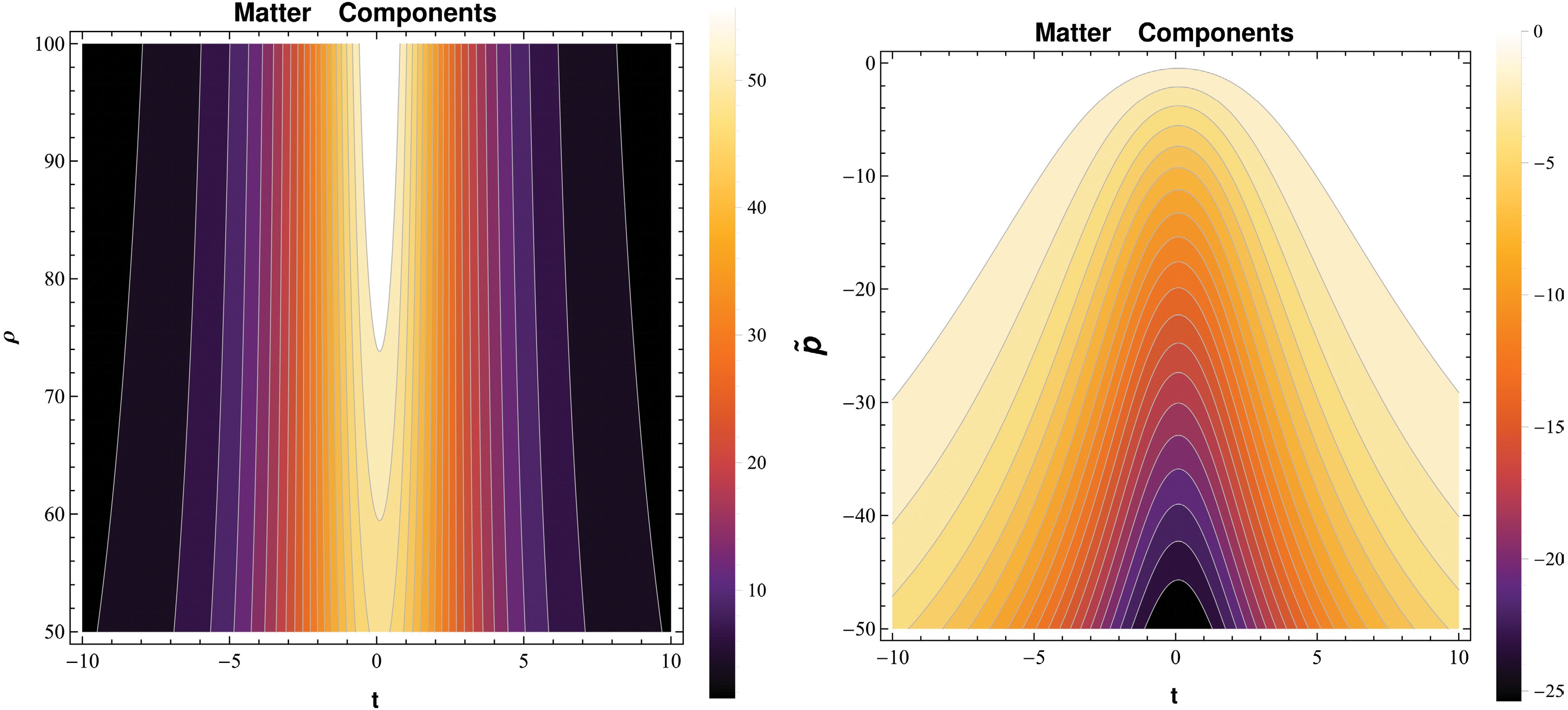
Figure 4.  (color online) Evolution of matter variables versus time.

In the present section, we examine how cosmic geometry is influenced by matter variables. Incorporating additional terms may yield significant outcomes. The examined bulk viscosity model offers a brief method for examining how various cosmic processes are affected by matter characteristics. Using Eq. (25) into Eqs. (23) and (27), we get the explicit expression of energy density and pressure

The dynamic evolution of energy density and pressure over time is shown in Fig. 4. This behavior depicts the evolution of the matter components corresponding to time. The energy density is symmetric about the bounce point and is positive throughout cosmic history. A large value of time leads to a higher energy density, suggesting that a stronger coupling encourages an immediate increase in energy density. Conversely, the pressure is negative and exhibits a bell-shaped behavior with a distinct minimum value at bounce, early and late times. Larger values of the parameter enhance the magnitude of this negative pressure and emphasize its indispensable part in cosmological dynamics. The presence of positive energy density coupled with a negative pressure results in the effective characteristics of exotic energy that exerts a repulsive force on a large scale. Consequently, these components are used to successfully realize scenarios for non-singular bouncing cosmology. The evolution of the matter variables is examined to verify the physical regularity of the cosmological solution. The finiteness of the energy density and pressure throughout cosmic evolution directly reflects the non-singular behavior of the scale factor and metric functions. This analysis is crucial, as a non-singular metric alone is not sufficient, a viable bouncing model must also ensure that all physical matter quantities remain bounded and well-defined across the bounce.

Figure 4.  (color online) Evolution of matter variables versus time.

The relationship between pressure and energy density is characterized by the EoS parameter, which is crucial to understand how the cosmos has evolved under various cosmological models. In bouncing cosmology, the dynamics of the EoS parameter are crucial because they determine how the cosmos changes during the compression, bounce and expansion epochs. The value of ω affects cosmic ability to bounce, avoid singularities and move smoothly between different stages. The EoS parameter is categorized by different stages of cosmic evolution. The matter characterized regions such as dust, radiative and stiff identified by $ \omega=0,\dfrac{1}{3} $, $ 1 $, respectively. On the other hand, the quintessence and phantom cosmic phases are given by $ \omega=-1 $, $ \omega <-1 $, $ -\dfrac{1}{3}<\omega<-1 $, respectively [58]. The expression of the EoS parameter in the presence of correction terms and viscous fluid is given by Fig. 5 depicts the behavior of the EoS parameter in this theoretical framework. It is noted that the EoS parameter is less than –1 during cosmic evolution, which suggests the phantom region. This behavior encodes a strong negative pressure from the modified gravity sector, contributing substantially to the accelerated expansion. However, for the smaller choice of model parameter, ω shifts from positive to negative values. The results indicate a shift in the EoS parameter from the dominated stiff matter phase to quintessence. This dynamical behavior of the ω shows a rich structure of the model, which plays an important role in driving the effective EoS, which helps in making smooth transitions between different cosmological epochs with satisfying the conditions needed for a stable and accelerating bouncing scenario. The effective EoS parameter is introduced to track the dynamical departure from standard matter behavior and to identify the regimes in which the null energy condition is violated. The evolution of the state parameter demonstrates a transient phantom-like phase near the bounce, which is a necessary feature for realizing a non-singular bounce in a homogeneous and isotropic universe.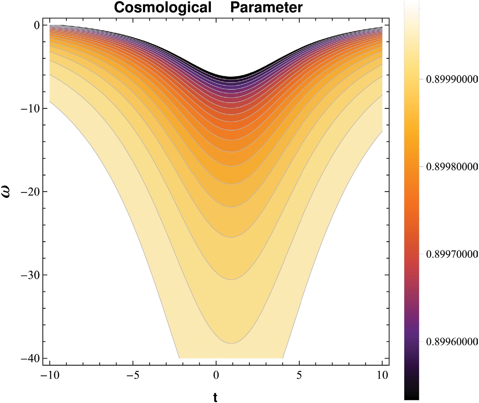

Figure 5.  (color online) Behavior of EoS parameter parameter against time.

The relationship between pressure and energy density is characterized by the EoS parameter, which is crucial to understand how the cosmos has evolved under various cosmological models. In bouncing cosmology, the dynamics of the EoS parameter are crucial because they determine how the cosmos changes during the compression, bounce and expansion epochs. The value of ω affects cosmic ability to bounce, avoid singularities and move smoothly between different stages. The EoS parameter is categorized by different stages of cosmic evolution. The matter characterized regions such as dust, radiative and stiff identified by $ \omega=0,\dfrac{1}{3} $, $ 1 $, respectively. On the other hand, the quintessence and phantom cosmic phases are given by $ \omega=-1 $, $ \omega <-1 $, $ -\dfrac{1}{3}<\omega<-1 $, respectively [58]. The expression of the EoS parameter in the presence of correction terms and viscous fluid is given by Fig. 5 depicts the behavior of the EoS parameter in this theoretical framework. It is noted that the EoS parameter is less than –1 during cosmic evolution, which suggests the phantom region. This behavior encodes a strong negative pressure from the modified gravity sector, contributing substantially to the accelerated expansion. However, for the smaller choice of model parameter, ω shifts from positive to negative values. The results indicate a shift in the EoS parameter from the dominated stiff matter phase to quintessence. This dynamical behavior of the ω shows a rich structure of the model, which plays an important role in driving the effective EoS, which helps in making smooth transitions between different cosmological epochs with satisfying the conditions needed for a stable and accelerating bouncing scenario. The effective EoS parameter is introduced to track the dynamical departure from standard matter behavior and to identify the regimes in which the null energy condition is violated. The evolution of the state parameter demonstrates a transient phantom-like phase near the bounce, which is a necessary feature for realizing a non-singular bounce in a homogeneous and isotropic universe.

Figure 5.  (color online) Behavior of EoS parameter parameter against time.

The behavior of ECs plays an essential role in determining whether the cosmological model is physically viable or not. The ECs are crucial for the development of geodesic structures that are light-like, time-like or space-like and identify the spacetime singularity. These constraints help us to understand cosmic geometry and its link with EMT. This yields energy density and pressure that contain contributions from both matter and geometry. As a result, even though this type of alteration may satisfy or violate ECs, its effects are contained within the context of a fluid. These energy constraints are formulated as four specific conditions, namely null energy constraint (NEC), strong energy constraints (SEC), weak energy constraints (WEC) and dominant energy constraints (DEC). These conditions are naturally changed by non-minimal couplings of geometry to matter in various MGTs. These conditions are expressed as

● NEC: $ \rho+\tilde{p}\geq 0 $

● WEC: $ \rho\geq 0 $, $ \rho+\tilde{p}\geq 0 $

● SEC: $ \rho+\tilde{p}\geq 0 $, $ \rho+3\tilde{p}\geq 0 $

● DEC: $ \rho\geq 0 $, $ \rho\geq |\tilde{p}| $

In the context of bouncing cosmology, the violation of the NEC near the bouncing epoch is a fundamental requirement for achieving a smooth transition from contraction to expansion. Modified gravity models can realize this violation through geometric corrections rather than involving exotic matter fields and thus physical self-consistency is preserved. The effective NEC violation leads to a positive time derivative of the Hubble parameter and non-singular bounce without divergent behavior in key cosmological quantities. At the same time other ECs, such as the weak and dominant ECs may be held in varying degrees of violation for different stages of evolution. This reflects a controlled, temporary departure from standard gravitational behavior. Furthermore, examining the evolution of energy limitations across several cosmic epochs provides crucial insights into the model's stability and thermodynamic feasibility. This dynamical behavior shows that MGT has potential useful way of resolving early universe singularities, compatible with the principles of classical energy when applied to subsequent cosmic evolution. The graphical behavior of ECs in relation to time is displayed in Fig. 6. The findings demonstrate that both NEC and SEC are violated near the bouncing epoch. The occurrence of a non-singular cosmic bounce requires these violations. The violation of the SEC is significant to cosmology as it decreases the gravitationally attractive properties of matter, which facilitates the transition from a contracting phase to an expanding phase. This theoretical behavior of ECs is the fundamental mechanism for constructing a stable, non-singular and efficient bouncing cosmic scenario. The violation of the null and strong ECs arises dynamically from the combined effects of matter-geometry coupling and bulk viscosity, rather than being imposed by hand. This violation is localized around the bounce and does not persist indefinitely, thereby avoiding pathological late-time behavior. This ensures that the energy condition analysis serves as the culmination of Section III, logically summarizing the physical mechanism responsible for the non-singular evolution.

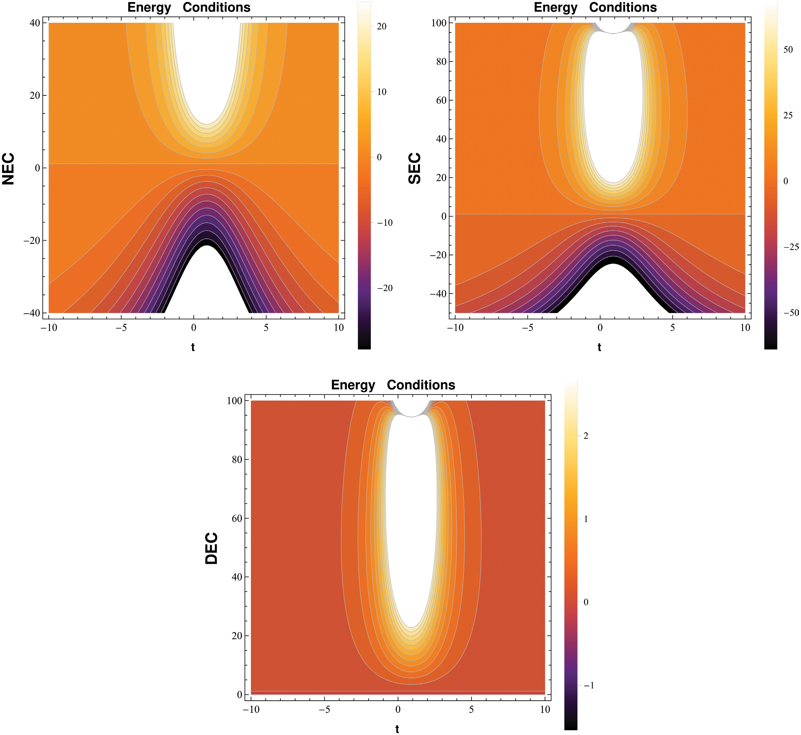
Figure 6.  (color online) Nature of ECs against time for various parametric values.

The behavior of ECs plays an essential role in determining whether the cosmological model is physically viable or not. The ECs are crucial for the development of geodesic structures that are light-like, time-like or space-like and identify the spacetime singularity. These constraints help us to understand cosmic geometry and its link with EMT. This yields energy density and pressure that contain contributions from both matter and geometry. As a result, even though this type of alteration may satisfy or violate ECs, its effects are contained within the context of a fluid. These energy constraints are formulated as four specific conditions, namely null energy constraint (NEC), strong energy constraints (SEC), weak energy constraints (WEC) and dominant energy constraints (DEC). These conditions are naturally changed by non-minimal couplings of geometry to matter in various MGTs. These conditions are expressed as

● NEC: $ \rho+\tilde{p}\geq 0 $

● WEC: $ \rho\geq 0 $, $ \rho+\tilde{p}\geq 0 $

● SEC: $ \rho+\tilde{p}\geq 0 $, $ \rho+3\tilde{p}\geq 0 $

● DEC: $ \rho\geq 0 $, $ \rho\geq |\tilde{p}| $

In the context of bouncing cosmology, the violation of the NEC near the bouncing epoch is a fundamental requirement for achieving a smooth transition from contraction to expansion. Modified gravity models can realize this violation through geometric corrections rather than involving exotic matter fields and thus physical self-consistency is preserved. The effective NEC violation leads to a positive time derivative of the Hubble parameter and non-singular bounce without divergent behavior in key cosmological quantities. At the same time other ECs, such as the weak and dominant ECs may be held in varying degrees of violation for different stages of evolution. This reflects a controlled, temporary departure from standard gravitational behavior. Furthermore, examining the evolution of energy limitations across several cosmic epochs provides crucial insights into the model's stability and thermodynamic feasibility. This dynamical behavior shows that MGT has potential useful way of resolving early universe singularities, compatible with the principles of classical energy when applied to subsequent cosmic evolution. The graphical behavior of ECs in relation to time is displayed in Fig. 6. The findings demonstrate that both NEC and SEC are violated near the bouncing epoch. The occurrence of a non-singular cosmic bounce requires these violations. The violation of the SEC is significant to cosmology as it decreases the gravitationally attractive properties of matter, which facilitates the transition from a contracting phase to an expanding phase. This theoretical behavior of ECs is the fundamental mechanism for constructing a stable, non-singular and efficient bouncing cosmic scenario. The violation of the null and strong ECs arises dynamically from the combined effects of matter-geometry coupling and bulk viscosity, rather than being imposed by hand. This violation is localized around the bounce and does not persist indefinitely, thereby avoiding pathological late-time behavior. This ensures that the energy condition analysis serves as the culmination of Section III, logically summarizing the physical mechanism responsible for the non-singular evolution.

Figure 6.  (color online) Nature of ECs against time for various parametric values.

In this section, our objective is to investigate the stability of our $ f(Q, {L}_{m}, T) $ gravity models. The sound speed is crucial to the classical stability of cosmological models and propagation of perturbations in MGTs. In the framework of $ f(Q,L_{m},T) $ gravity, the speed of sound is given by $ C_{s}^{2}=\dfrac{\dot{\tilde{p}}}{\dot{\rho}} $, where $ \tilde{p} $ and ρ are respectively the pressure and energy density coming from a non-metric coupling between non-metricity, matter Lagrangian and trace of EMT. Since the velocity of sound $ C_{s}^{2} $ requires to remain positive in a physical system that is mechanically or thermodynamically stable, a model is considered viable when $ C_{s}^{2}>0 $. Additionally, to provide mechanical stability, $ C_{s}^{2} $ must equal or be less than 1. The interval $ 0\leq C_{s}^{2}\leq 1 $ characterizes the stability whereas $ C_{s}^{2}\geq 1 $ will result in an unstable model.

The behavior of $ C_{s}^{2} $ over the time is a vital parameter of stability of bouncing cosmology as shown graphically in Fig. 7. For all of the expansion the condition $ 0 <C_{s}^{2}<1 $ is fulfilled and thus it is consistent with not having classical instabilities and maintaining causality. When the bounce is near, $ C_{s}^{2} $ monotonically decreases as a function of time and reaches its minimum value which means the effective cosmic fluid is slightly softening temporarily due to the gravitational and viscous strong effects around this period $ (t=0) $. After the bounce, $ C_{s}^{2} $ increases again to its usual value which indicates a stability restoration in the universe from contraction to expansion phase. The symmetric character around the bounce of the plot indicates the microphysical properties of cosmic fluid are well-behaved and continue across contracting and expanding phases that support the physical validity of our model. A stable and a causal bouncing solution, which is not always apparent in alternative cosmologies is supported by the sound speed behavior during the cosmic evolution. In the usual GR-based bounce settings, stability may be attained after including exotic matter which cause a $ C_s^{2}<0 $ and indicates classical instabilities. Similarly, in certain phantom-driven and ekpyrotic models, causality could be violated in superluminal regions. Loop Quantum Cosmology uses quantum corrections to increase stability close to the bounce, however this depends on high-energy quantum processes whose classical limit is unclear. In contrast, the modified $ f(Q,L_{m},T) $ gravity exhibits a smooth sound speed without the use of an exotic field or quantum correction of gravity, demonstrating that bounce might be achieved through the efficient connection of the viscous mechanism and matter-geometry while maintaining both physical intuitions.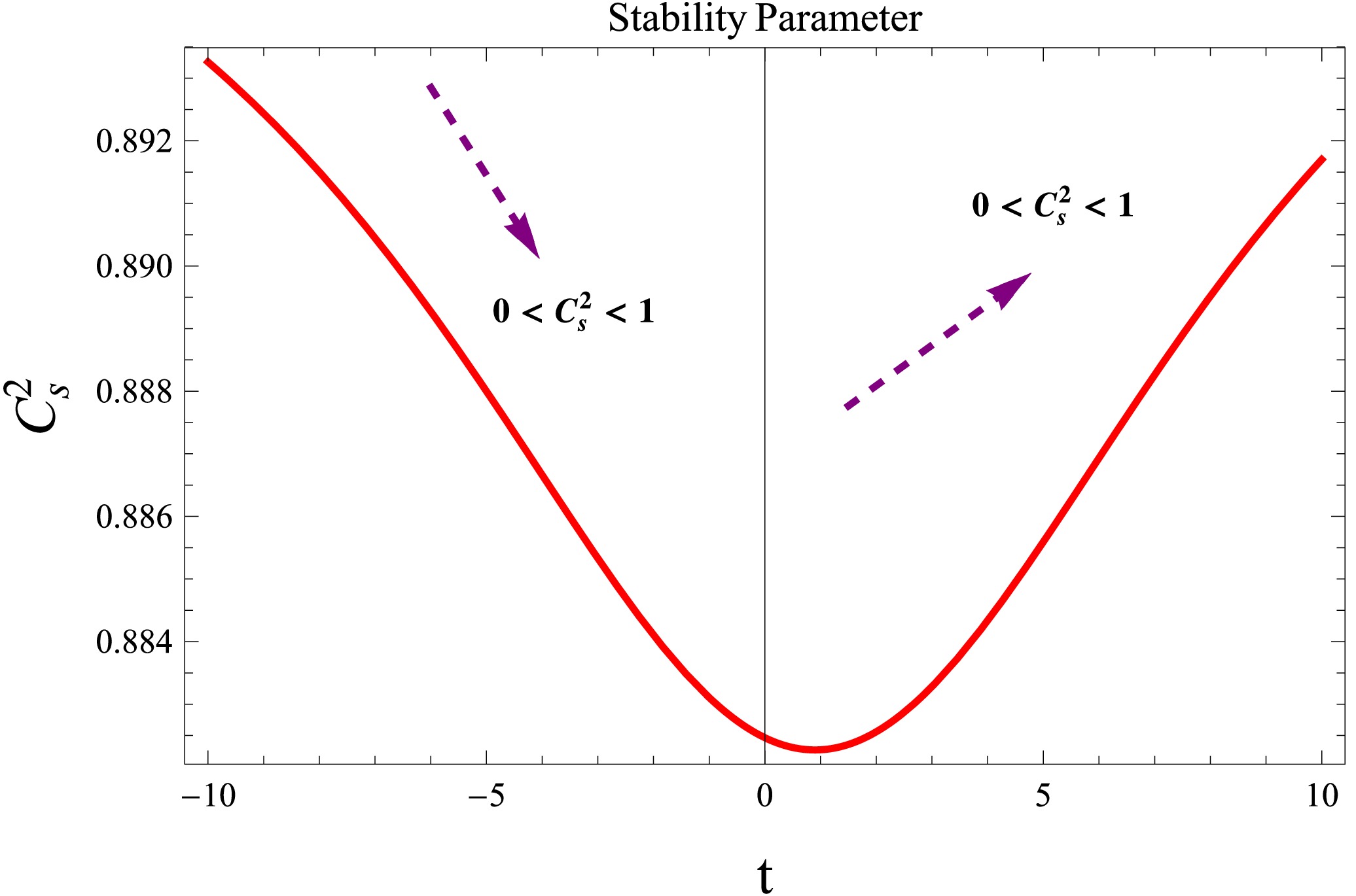

Figure 7.  (color online) Graph of squared sound speed corresponding to time.

In this section, our objective is to investigate the stability of our $ f(Q, {L}_{m}, T) $ gravity models. The sound speed is crucial to the classical stability of cosmological models and propagation of perturbations in MGTs. In the framework of $ f(Q,L_{m},T) $ gravity, the speed of sound is given by $ C_{s}^{2}=\dfrac{\dot{\tilde{p}}}{\dot{\rho}} $, where $ \tilde{p} $ and ρ are respectively the pressure and energy density coming from a non-metric coupling between non-metricity, matter Lagrangian and trace of EMT. Since the velocity of sound $ C_{s}^{2} $ requires to remain positive in a physical system that is mechanically or thermodynamically stable, a model is considered viable when $ C_{s}^{2}>0 $. Additionally, to provide mechanical stability, $ C_{s}^{2} $ must equal or be less than 1. The interval $ 0\leq C_{s}^{2}\leq 1 $ characterizes the stability whereas $ C_{s}^{2}\geq 1 $ will result in an unstable model.

The behavior of $ C_{s}^{2} $ over the time is a vital parameter of stability of bouncing cosmology as shown graphically in Fig. 7. For all of the expansion the condition $ 0 <C_{s}^{2}<1 $ is fulfilled and thus it is consistent with not having classical instabilities and maintaining causality. When the bounce is near, $ C_{s}^{2} $ monotonically decreases as a function of time and reaches its minimum value which means the effective cosmic fluid is slightly softening temporarily due to the gravitational and viscous strong effects around this period $ (t=0) $. After the bounce, $ C_{s}^{2} $ increases again to its usual value which indicates a stability restoration in the universe from contraction to expansion phase. The symmetric character around the bounce of the plot indicates the microphysical properties of cosmic fluid are well-behaved and continue across contracting and expanding phases that support the physical validity of our model. A stable and a causal bouncing solution, which is not always apparent in alternative cosmologies is supported by the sound speed behavior during the cosmic evolution. In the usual GR-based bounce settings, stability may be attained after including exotic matter which cause a $ C_s^{2}<0 $ and indicates classical instabilities. Similarly, in certain phantom-driven and ekpyrotic models, causality could be violated in superluminal regions. Loop Quantum Cosmology uses quantum corrections to increase stability close to the bounce, however this depends on high-energy quantum processes whose classical limit is unclear. In contrast, the modified $ f(Q,L_{m},T) $ gravity exhibits a smooth sound speed without the use of an exotic field or quantum correction of gravity, demonstrating that bounce might be achieved through the efficient connection of the viscous mechanism and matter-geometry while maintaining both physical intuitions.

Figure 7.  (color online) Graph of squared sound speed corresponding to time.

The higher-order cosmography is a technique in cosmology that extends traditional cosmographic methods by utilizing higher-degree derivatives of the Hubble parameter. The time-varying scale factor, which shows how cosmic distances change over time, would be used to investigate cosmic expansion and the large-scale structure. We examine the dynamics of cosmic expansion by taking into account scale-factor derivatives that go beyond Hubble and deceleration parameters. These high-order derivatives are very helpful in comprehending the behavior of cosmic evaluation. These cosmographic parameters are defined as

Here, jerk, snap, lerk and maxout are represented by $ J, S, L $, and M, respectively. Figure 8 shows the temporal behavior of higher-order cosmographic parameters such as jerk, snap, lerk and maxout with respect to time which offers a deeper understanding of the dynamical trajectories experienced by the bouncing universe. Around the bounce epoch $ (t=0) $, all the parameters exhibit rapid spikes, signifying a quick dynamics as the cosmos transitions from contraction to expansion. In the far field from the bounce, these parameters become slowly evolving toward approximately constant values, which corresponds to a smoother and more regular regime of expansion. A symmetric behavior about the bounce indicates time-reversal invariance of cosmic evolution while the peaks are finite (i.e. non-singular) near the transition. The bounce is dynamical and regulated as demonstrated by these second-order diagnostics. Thus, it is driven by powerful but necessary mechanical influences, such as those caused by viscous processes and changed gravity.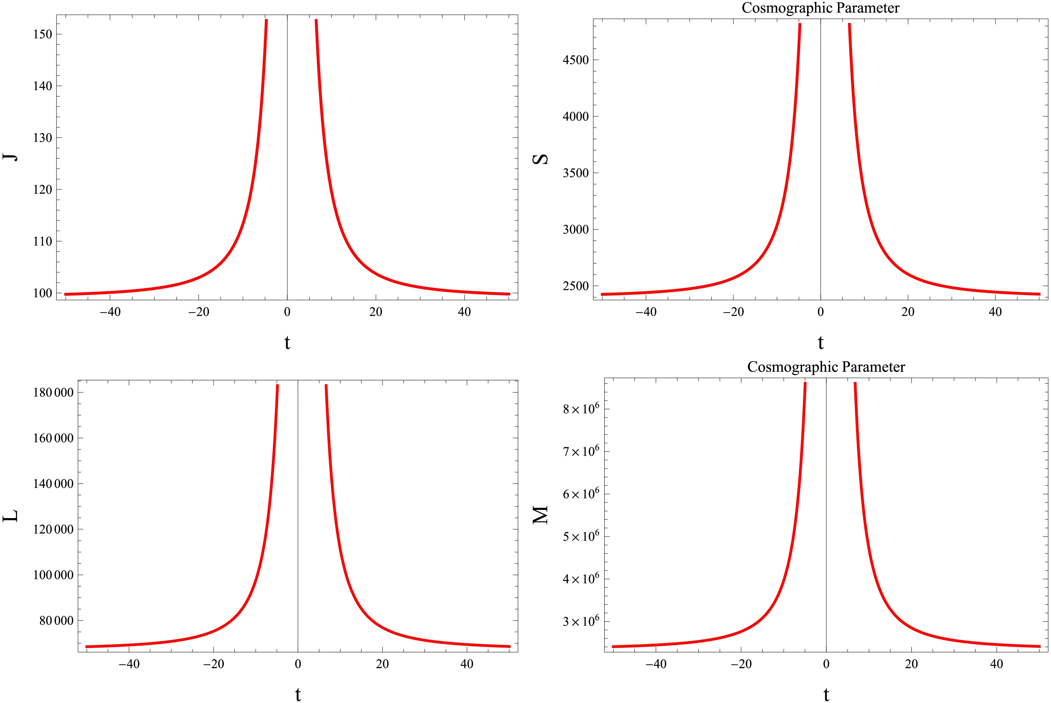

Figure 8.  (color online) Plots of cosmographic parameters versus time.

The higher-order cosmography is a technique in cosmology that extends traditional cosmographic methods by utilizing higher-degree derivatives of the Hubble parameter. The time-varying scale factor, which shows how cosmic distances change over time, would be used to investigate cosmic expansion and the large-scale structure. We examine the dynamics of cosmic expansion by taking into account scale-factor derivatives that go beyond Hubble and deceleration parameters. These high-order derivatives are very helpful in comprehending the behavior of cosmic evaluation. These cosmographic parameters are defined as

Here, jerk, snap, lerk and maxout are represented by $ J, S, L $, and M, respectively. Figure 8 shows the temporal behavior of higher-order cosmographic parameters such as jerk, snap, lerk and maxout with respect to time which offers a deeper understanding of the dynamical trajectories experienced by the bouncing universe. Around the bounce epoch $ (t=0) $, all the parameters exhibit rapid spikes, signifying a quick dynamics as the cosmos transitions from contraction to expansion. In the far field from the bounce, these parameters become slowly evolving toward approximately constant values, which corresponds to a smoother and more regular regime of expansion. A symmetric behavior about the bounce indicates time-reversal invariance of cosmic evolution while the peaks are finite (i.e. non-singular) near the transition. The bounce is dynamical and regulated as demonstrated by these second-order diagnostics. Thus, it is driven by powerful but necessary mechanical influences, such as those caused by viscous processes and changed gravity.

Figure 8.  (color online) Plots of cosmographic parameters versus time.

The second law of thermodynamics is fundamental for an analysis of the physical acceptability of bouncing cosmological models, especially when classical singularities are avoided. In a regular bounce, the universe goes through from contraction to expansion and it is being thermodynamically well-behaved due to the implementation of the second law, so that physical causality does not violate the time arrow. With this justification, an effective horizon entropy and its associated temperature are assigned to the cosmological or apparent horizon, respectively by which one can check whether or not total entropy of the universe is increasing monotonically during the bouncing stage. This requirement yields a strong model-independent constraint on MGTs and matter couplings just like its role in black hole thermodynamics. In this way, studying thermodynamics laws in bouncing cosmology provides deeper knowledge about the micro-physical consistency of the theory and claims for application of entropy and temperature relations such as those inspired by Hawking radiation to characterize horizon dynamics even beyond the general relativistic framework. We further emphasize that the goal of this section is not to derive a new Hawking temperature law, but rather to examine whether the bouncing cosmological solutions obtained in the preceding sections remain compatible with the generalized second law of thermodynamics when standard horizon thermodynamics is assumed.

The cosmic dynamics is characterized by the generalized second law of thermodynamics, which specifies that the total entropy generation in a closed system cannot diminish, it may only remain constant or increase over time. In bouncing cosmology, it is crucial to investigate the dynamics of entropy formation in both the contracting and expanding phases. Furthermore, with the increase of Hawking temperature, it can be seen clearly that system approaches to equilibrium for cosmic expansion. This increment in temperature allows for the theoretical observation of reheating after a cosmological bounce. The correlation between Hawking temperature behavior and entropy production indicates that bulk viscosity is crucial for achieving a thermodynamically viable cosmic bounce. The integrated thermodynamic modifications provide compelling evidence of the model's efficiency in addressing cosmic singularities through conventional thermodynamic approaches. The total cosmic entropy is composed of the matter contribution within the horizon ($ {\mathbb{S}}_{\text{in}} $) plus the entropy at its boundary ($ {\mathbb{S}}_{\text{on}} $). In this consideration the boundary of cosmos is defined by apparent horizon with radius described through Hubble parameter Eq. (17) as

The entropy which is associated with the horizon surface area, is described as

In this case, $ {\mathbb{K}}_b $ represents the Boltzmann constant, $ {\mathbb{L}}_{\tilde{p}} $ represents the Planck length, and $ {\mathbb{A}}=4\pi {\mathbb{R}}_{H}^{2} $ represents the cosmic horizon section. Therefore, utilizing Eqs. (32) and (33), we obtain

According to Gibb's relation, the entropy of matter enclosed within the horizon is expressed as

At the horizon's edge, the Hawking temperature $ ({\mathbb{T}}_H) $ is defined. It is possible to compute the volume inside the apparent horizon as

By combining Eqs. (35) and (36), we derive

The second principle of thermodynamics states that since the positive entropy ($ {\mathbb{S}}_{\text{in}}>0 $) of the material inside the horizon, the cosmic total entropy should increase steadily. The definition of total entropy is expressed as

The overall cosmic entropy increases with time as shown in Fig. 9, which also shows the rising Hawking temperature following the bounce phase. The basic principles of cosmic thermodynamics and the compatibility of entropy creation are demonstrated by this behavior. Additionally, the increasing Hawking temperature shows that the system is progressing towards equilibrium throughout the expansion phase. This increase in temperature is consistent with theoretical findings for reheating processes that occur after a cosmic bounce. The total entropy, including both horizon and matter contributions, is shown to be a monotonically increasing function of time throughout the evolution, including in the vicinity of the bounce. This result demonstrates that the non-singular bouncing solutions obtained in the present $ f(Q,L_{m},T) $ model are thermodynamically consistent and do not violate the generalized second law, despite the presence of energy condition violations at the background level. This result is non-trivial, as bouncing cosmologies often suffer from thermodynamic inconsistencies or entropy decrease near the bounce. In order to have a non-singular bounce, these inputs result in the creation of entropy, which maintains thermodynamic consistency even when the standard ECs are not satisfied. Unlike the ΛCDM scenario, where entropy production is usually small, the present model exhibits a multiscale thermodynamic structure with corrections due to coupling being crucial in determining the evolution of the primordial universe.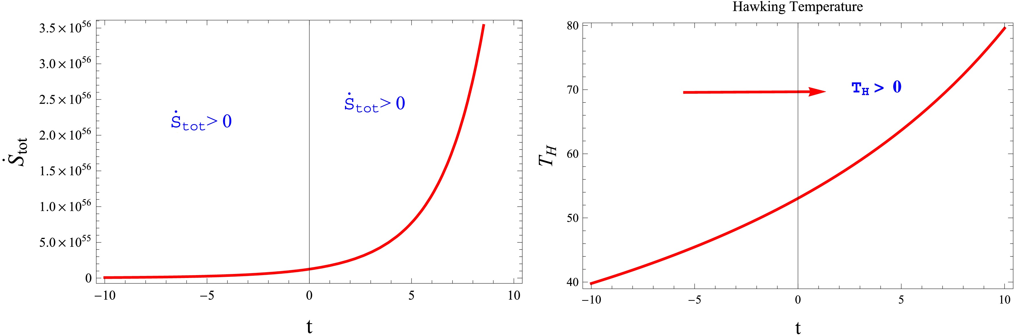

Figure 9.  (color online) Behavior of entropy and Hawking temperature with respect to time.

The second law of thermodynamics is fundamental for an analysis of the physical acceptability of bouncing cosmological models, especially when classical singularities are avoided. In a regular bounce, the universe goes through from contraction to expansion and it is being thermodynamically well-behaved due to the implementation of the second law, so that physical causality does not violate the time arrow. With this justification, an effective horizon entropy and its associated temperature are assigned to the cosmological or apparent horizon, respectively by which one can check whether or not total entropy of the universe is increasing monotonically during the bouncing stage. This requirement yields a strong model-independent constraint on MGTs and matter couplings just like its role in black hole thermodynamics. In this way, studying thermodynamics laws in bouncing cosmology provides deeper knowledge about the micro-physical consistency of the theory and claims for application of entropy and temperature relations such as those inspired by Hawking radiation to characterize horizon dynamics even beyond the general relativistic framework. We further emphasize that the goal of this section is not to derive a new Hawking temperature law, but rather to examine whether the bouncing cosmological solutions obtained in the preceding sections remain compatible with the generalized second law of thermodynamics when standard horizon thermodynamics is assumed.

The cosmic dynamics is characterized by the generalized second law of thermodynamics, which specifies that the total entropy generation in a closed system cannot diminish, it may only remain constant or increase over time. In bouncing cosmology, it is crucial to investigate the dynamics of entropy formation in both the contracting and expanding phases. Furthermore, with the increase of Hawking temperature, it can be seen clearly that system approaches to equilibrium for cosmic expansion. This increment in temperature allows for the theoretical observation of reheating after a cosmological bounce. The correlation between Hawking temperature behavior and entropy production indicates that bulk viscosity is crucial for achieving a thermodynamically viable cosmic bounce. The integrated thermodynamic modifications provide compelling evidence of the model's efficiency in addressing cosmic singularities through conventional thermodynamic approaches. The total cosmic entropy is composed of the matter contribution within the horizon ($ {\mathbb{S}}_{\text{in}} $) plus the entropy at its boundary ($ {\mathbb{S}}_{\text{on}} $). In this consideration the boundary of cosmos is defined by apparent horizon with radius described through Hubble parameter Eq. (17) as

The entropy which is associated with the horizon surface area, is described as

In this case, $ {\mathbb{K}}_b $ represents the Boltzmann constant, $ {\mathbb{L}}_{\tilde{p}} $ represents the Planck length, and $ {\mathbb{A}}=4\pi {\mathbb{R}}_{H}^{2} $ represents the cosmic horizon section. Therefore, utilizing Eqs. (32) and (33), we obtain

According to Gibb's relation, the entropy of matter enclosed within the horizon is expressed as

At the horizon's edge, the Hawking temperature $ ({\mathbb{T}}_H) $ is defined. It is possible to compute the volume inside the apparent horizon as

By combining Eqs. (35) and (36), we derive

The second principle of thermodynamics states that since the positive entropy ($ {\mathbb{S}}_{\text{in}}>0 $) of the material inside the horizon, the cosmic total entropy should increase steadily. The definition of total entropy is expressed as

The overall cosmic entropy increases with time as shown in Fig. 9, which also shows the rising Hawking temperature following the bounce phase. The basic principles of cosmic thermodynamics and the compatibility of entropy creation are demonstrated by this behavior. Additionally, the increasing Hawking temperature shows that the system is progressing towards equilibrium throughout the expansion phase. This increase in temperature is consistent with theoretical findings for reheating processes that occur after a cosmic bounce. The total entropy, including both horizon and matter contributions, is shown to be a monotonically increasing function of time throughout the evolution, including in the vicinity of the bounce. This result demonstrates that the non-singular bouncing solutions obtained in the present $ f(Q,L_{m},T) $ model are thermodynamically consistent and do not violate the generalized second law, despite the presence of energy condition violations at the background level. This result is non-trivial, as bouncing cosmologies often suffer from thermodynamic inconsistencies or entropy decrease near the bounce. In order to have a non-singular bounce, these inputs result in the creation of entropy, which maintains thermodynamic consistency even when the standard ECs are not satisfied. Unlike the ΛCDM scenario, where entropy production is usually small, the present model exhibits a multiscale thermodynamic structure with corrections due to coupling being crucial in determining the evolution of the primordial universe.

Figure 9.  (color online) Behavior of entropy and Hawking temperature with respect to time.

The conventional cosmological model, which is widely accepted, has been successful in explaining the cosmic evolution and large-scale structure, regardless of certain inconsistencies. One of the main issues in the early phases of cosmic evolution has been the singularity problem. The cosmos contracts before expanding and experiencing a singularity in the bouncing cosmology, which is thought to offer a compelling answer to counter this issue. In MGTs, bouncing cosmology is achieved by altering the curvature or matter content. The bounce offers an essentially seamless and possibly non-singular transition between two cosmic epochs in this perspective. Incorporating bulk viscosity, which is not only retain the fluctuations but also supports a more realistic and feasible cosmology, is one potential solution for such a bounce. Bulk viscosity has a significant impact on cosmic characteristics and generalizes ideal fluid assumptions. In this study, we investigate how an extended theory of gravity can give rise to viable cosmological models capable of explaining the late-time accelerated expansion of the universe while simultaneously accommodating a non-singular bouncing scenario. The MGTs have been widely proposed as alternatives to GR, offering diverse geometric mechanisms to describe cosmic evolution and the effective nature of DE.

In this context, we focus on the $ f(Q,L_{m},T) $ gravity framework, where the gravitational action depends on the non-metricity scalar Q, the matter Lagrangian $ L_{m} $ and the trace of the EMT. Specifically, we consider the linear functional form $ f(Q,L_{m},T) =Q+\sigma_{1}L_{m}+\sigma_{2}T $ with $ \sigma_{1} $ and $ \sigma_{2} $ being constant coupling parameters. We analyze how the explicit matter-geometry coupling introduced through $ L_{m} $ and T influences the cosmic dynamics and facilitates a non-singular bounce without invoking additional exotic matter components. In this work, we discuss the various cosmic bounce scenarios in the context of $ f(Q,L_{m},T) $ gravity by analyzing the resulting cosmic dynamics in the presence of viscous matter. The field equations are solved by examining the temporal behavior of key kinematical parameters, including the deceleration, adiabatic speed of sound, jerk, snap, and lerk parameters. Moreover, we can simulate dissipation processes in the early universe by including bulk viscous effects to a perfect fluid. This makes it possible to utilize our model directly to describe cosmic dynamics, which is essential for comprehending the development of the late-time direction of time in bouncing models. Additionally, the model serves as an evaluation platform for geometric entropy production models and could potentially establish a link between gravity-side and thermodynamic irreversibility, which is a fascinating problem in cosmology overall. Our main findings are as follows.

● The Hubble parameter effectively shows the post-bounce expansion (left panel of Fig. 1), the transition at the bouncing epoch ($ H=0 $) and the pre-bounce cosmic contraction. The continuous change from a contraction to an expanding phase of the cosmic bounce is highlighted by the time derivative of the Hubble parameter (right panel of Fig. 1).

● The scale factor is positive and finite at all times during cosmic evolution, which ensures that there is no big bang like singularity as shown in Fig. 2. It describes a symmetric bounce at $ t=0 $, connecting a smooth contracting phase $ (t<0) $ to a expanding universe $ (t>0) $.

● A crucial factor in comparing the model to the observable reality of cosmic expansion is the deceleration parameter. The extended periods of accelerated expansion in the pre and post-bounce eras are shown by its negative values on both sides of the bounce (Fig. 3) which is consistent with typical cosmology predictions (Table 1).

● Accelerated cosmic expansion is indicated by the positive energy density and negative pressure profile traits. The realistic non-singular bouncing cosmology is supported by the behavior of this unique matter variable (Fig. 4).

● Additionally, the EoS parameter shows the change from an early state dominated by stiff matter to an expansion era. The way this parameter data behaves validates our analysis, which shows how quickly the universe is expanding (Fig. 5).

● The examination of ECs demonstrates the presence of feasible bouncing solutions (Fig. 6). The violation of ECs is essential for facilitating cosmological bouncing models and substantiates their physical validity in elucidating the cosmic dynamics.

● The stability and causality of the bouncing model are demonstrated by the fact that $ 0<C_s^{2}<1 $ during all cosmic eras (Fig. 7). Although it does not have destabilizing effects, the symmetric minimum of this spectrum around the bounce stage.

● Moreover, the behavior of cosmographic parameters are shown in Fig. 8. The rapid non-singular change from a shrinking to an expanding phase is representative of the sharp peaks in jerk, snap, lerk, and maxout at the bounce. The existence of a time-reversal symmetric bouncing cosmology is confirmed by its bounded, symmetric nature.

● The increase in entropy formation around the bouncing epoch indicates a smooth transition between contracting and expanding cycles, which ensures that cosmic acceleration is in accordance with the generalized second law of thermodynamics (left plot of Fig. 9). The increasing Hawking temperature highlights the function of bulk viscosity in maintaining a thermodynamic bouncing cosmology while avoiding the singularities and indicates equilibrium in the expanding period (right plot of Fig. 9).

Several studies have explored cosmological models, such as bulk viscous fluids in both MGT and GR contexts. These studies usually use basic viscosity coefficients like $ \varepsilon=const $ or forms proportional to the energy density or Hubble parameter. The current study is distinctive in a way that it uses a time-dependent viscosity coefficient of the type $ \varepsilon=\varepsilon_{0}(t-\tau_{0})^{-2n}H $ in the context of gravity $ f(Q,L_{m},T) $. It is inspired by the thermodynamic behavior of the early universe, where dissipative phenomena were dominating at first but progressively disappeared as the universe expanded. The exponent connects early-universe viscous scales with late-time fluid behavior by acting as an adjustable parameter that regulates the rate at which the bulk viscosity decays. The time dependent viscosity coefficient adds an effective negative pressure contribution which is important in the early universe and naturally decays at large times. Our model physically motivated viscous effects generically lead to a non-singular cosmological evolution with modified gravitational dynamics and it asymptotically reaches the standard weakly dissipative scenario that is consistent with ΛCDM-like expansion in late universe. This makes this the immediate and natural generalization of ΛCDM, maintaining its observational successes while furnishing a more complete and richer description of early time cosmic dynamics. The avoidance of the big bang singularity is achieved through dynamically induced violations of the null energy condition arising from matter-geometry coupling and bulk viscosity, rather than through ad hoc exotic matter components. The satisfaction of the generalized second law of thermodynamics across the bounce provides an important consistency check that supports the physical viability of the model at the background level.

In modified symmetric teleparallel gravity, the extension from $ f(Q) $ to matter-geometry coupled forms such as $ f(Q,T) $, $ f(Q,L_{m}) $ and $ f(Q,L_{m},T) $ reflects a progressive enrichment of the interaction between spacetime and matter. The $ f(Q,L_{m}) $ framework introduces an explicit dependence on the matter Lagrangian which allows a direct coupling between non-metricity and the microscopic properties of matter, which can modify conservation laws and lead to extra force terms affecting particle motion.The $ f(Q,T) $ gravity couples non-metricity to the trace of EMT, effectively encoding macroscopic matter effects and enabling phenomenological explanations of late time cosmic acceleration without involving dark energy though at the cost of potential ambiguities related to matter sector definitions. In contrast, the generalized $ f(Q,L_{m},T) $ theory unifies both approaches by incorporating dependence on both matter Lagrangian and trace of EMT that provides a more comprehensive framework to capture dissipative processes, bulk viscous effects and non-equilibrium thermodynamics in cosmology. Furthermore, this cohesive coupling enhances the flexibility of model and is capable of accounting for deviations from energy-momentum conservation, cosmic acceleration and complex matter interactions at the fundamental level, making it a more powerful and more constrained theory that requires thoroughly consistency checks to avoid model instabilities and guarantee its physical viability.

The conventional cosmological model, which is widely accepted, has been successful in explaining the cosmic evolution and large-scale structure, regardless of certain inconsistencies. One of the main issues in the early phases of cosmic evolution has been the singularity problem. The cosmos contracts before expanding and experiencing a singularity in the bouncing cosmology, which is thought to offer a compelling answer to counter this issue. In MGTs, bouncing cosmology is achieved by altering the curvature or matter content. The bounce offers an essentially seamless and possibly non-singular transition between two cosmic epochs in this perspective. Incorporating bulk viscosity, which is not only retain the fluctuations but also supports a more realistic and feasible cosmology, is one potential solution for such a bounce. Bulk viscosity has a significant impact on cosmic characteristics and generalizes ideal fluid assumptions. In this study, we investigate how an extended theory of gravity can give rise to viable cosmological models capable of explaining the late-time accelerated expansion of the universe while simultaneously accommodating a non-singular bouncing scenario. The MGTs have been widely proposed as alternatives to GR, offering diverse geometric mechanisms to describe cosmic evolution and the effective nature of DE.

In this context, we focus on the $ f(Q,L_{m},T) $ gravity framework, where the gravitational action depends on the non-metricity scalar Q, the matter Lagrangian $ L_{m} $ and the trace of the EMT. Specifically, we consider the linear functional form $ f(Q,L_{m},T) =Q+\sigma_{1}L_{m}+\sigma_{2}T $ with $ \sigma_{1} $ and $ \sigma_{2} $ being constant coupling parameters. We analyze how the explicit matter-geometry coupling introduced through $ L_{m} $ and T influences the cosmic dynamics and facilitates a non-singular bounce without invoking additional exotic matter components. In this work, we discuss the various cosmic bounce scenarios in the context of $ f(Q,L_{m},T) $ gravity by analyzing the resulting cosmic dynamics in the presence of viscous matter. The field equations are solved by examining the temporal behavior of key kinematical parameters, including the deceleration, adiabatic speed of sound, jerk, snap, and lerk parameters. Moreover, we can simulate dissipation processes in the early universe by including bulk viscous effects to a perfect fluid. This makes it possible to utilize our model directly to describe cosmic dynamics, which is essential for comprehending the development of the late-time direction of time in bouncing models. Additionally, the model serves as an evaluation platform for geometric entropy production models and could potentially establish a link between gravity-side and thermodynamic irreversibility, which is a fascinating problem in cosmology overall. Our main findings are as follows.

● The Hubble parameter effectively shows the post-bounce expansion (left panel of Fig. 1), the transition at the bouncing epoch ($ H=0 $) and the pre-bounce cosmic contraction. The continuous change from a contraction to an expanding phase of the cosmic bounce is highlighted by the time derivative of the Hubble parameter (right panel of Fig. 1).

● The scale factor is positive and finite at all times during cosmic evolution, which ensures that there is no big bang like singularity as shown in Fig. 2. It describes a symmetric bounce at $ t=0 $, connecting a smooth contracting phase $ (t<0) $ to a expanding universe $ (t>0) $.

● A crucial factor in comparing the model to the observable reality of cosmic expansion is the deceleration parameter. The extended periods of accelerated expansion in the pre and post-bounce eras are shown by its negative values on both sides of the bounce (Fig. 3) which is consistent with typical cosmology predictions (Table 1).

● Accelerated cosmic expansion is indicated by the positive energy density and negative pressure profile traits. The realistic non-singular bouncing cosmology is supported by the behavior of this unique matter variable (Fig. 4).

● Additionally, the EoS parameter shows the change from an early state dominated by stiff matter to an expansion era. The way this parameter data behaves validates our analysis, which shows how quickly the universe is expanding (Fig. 5).

● The examination of ECs demonstrates the presence of feasible bouncing solutions (Fig. 6). The violation of ECs is essential for facilitating cosmological bouncing models and substantiates their physical validity in elucidating the cosmic dynamics.

● The stability and causality of the bouncing model are demonstrated by the fact that $ 0<C_s^{2}<1 $ during all cosmic eras (Fig. 7). Although it does not have destabilizing effects, the symmetric minimum of this spectrum around the bounce stage.

● Moreover, the behavior of cosmographic parameters are shown in Fig. 8. The rapid non-singular change from a shrinking to an expanding phase is representative of the sharp peaks in jerk, snap, lerk, and maxout at the bounce. The existence of a time-reversal symmetric bouncing cosmology is confirmed by its bounded, symmetric nature.

● The increase in entropy formation around the bouncing epoch indicates a smooth transition between contracting and expanding cycles, which ensures that cosmic acceleration is in accordance with the generalized second law of thermodynamics (left plot of Fig. 9). The increasing Hawking temperature highlights the function of bulk viscosity in maintaining a thermodynamic bouncing cosmology while avoiding the singularities and indicates equilibrium in the expanding period (right plot of Fig. 9).

Several studies have explored cosmological models, such as bulk viscous fluids in both MGT and GR contexts. These studies usually use basic viscosity coefficients like $ \varepsilon=const $ or forms proportional to the energy density or Hubble parameter. The current study is distinctive in a way that it uses a time-dependent viscosity coefficient of the type $ \varepsilon=\varepsilon_{0}(t-\tau_{0})^{-2n}H $ in the context of gravity $ f(Q,L_{m},T) $. It is inspired by the thermodynamic behavior of the early universe, where dissipative phenomena were dominating at first but progressively disappeared as the universe expanded. The exponent connects early-universe viscous scales with late-time fluid behavior by acting as an adjustable parameter that regulates the rate at which the bulk viscosity decays. The time dependent viscosity coefficient adds an effective negative pressure contribution which is important in the early universe and naturally decays at large times. Our model physically motivated viscous effects generically lead to a non-singular cosmological evolution with modified gravitational dynamics and it asymptotically reaches the standard weakly dissipative scenario that is consistent with ΛCDM-like expansion in late universe. This makes this the immediate and natural generalization of ΛCDM, maintaining its observational successes while furnishing a more complete and richer description of early time cosmic dynamics. The avoidance of the big bang singularity is achieved through dynamically induced violations of the null energy condition arising from matter-geometry coupling and bulk viscosity, rather than through ad hoc exotic matter components. The satisfaction of the generalized second law of thermodynamics across the bounce provides an important consistency check that supports the physical viability of the model at the background level.

In modified symmetric teleparallel gravity, the extension from $ f(Q) $ to matter-geometry coupled forms such as $ f(Q,T) $, $ f(Q,L_{m}) $ and $ f(Q,L_{m},T) $ reflects a progressive enrichment of the interaction between spacetime and matter. The $ f(Q,L_{m}) $ framework introduces an explicit dependence on the matter Lagrangian which allows a direct coupling between non-metricity and the microscopic properties of matter, which can modify conservation laws and lead to extra force terms affecting particle motion.The $ f(Q,T) $ gravity couples non-metricity to the trace of EMT, effectively encoding macroscopic matter effects and enabling phenomenological explanations of late time cosmic acceleration without involving dark energy though at the cost of potential ambiguities related to matter sector definitions. In contrast, the generalized $ f(Q,L_{m},T) $ theory unifies both approaches by incorporating dependence on both matter Lagrangian and trace of EMT that provides a more comprehensive framework to capture dissipative processes, bulk viscous effects and non-equilibrium thermodynamics in cosmology. Furthermore, this cohesive coupling enhances the flexibility of model and is capable of accounting for deviations from energy-momentum conservation, cosmic acceleration and complex matter interactions at the fundamental level, making it a more powerful and more constrained theory that requires thoroughly consistency checks to avoid model instabilities and guarantee its physical viability.