


 Abstract
 HTML
 Reference
 Related
 PDF



-
General Relativity (GR) continues to be the most robust and widely accepted theory for explaining gravity, particularly in regimes characterized by strong gravitational fields, despite unresolved issues such as singularities and the lack of spacetime quantization. One of the profound predictions of GR is the gravitational collapse of massive stars at the end of their life cycles, leading to the formation of black hole (BH) solutions to Einstein's field equations that exhibit remarkable gravitational features. Recent advances in observational astronomy have provided compelling evidence supporting GR's predictions in the strong-field regime. The Event Horizon Telescope (EHT) collaboration successfully captured the shadow of the supermassive BH at the center of the galaxy M87 (M87*) and Sagittarius A* (Sgr A*) [1, 2], while the LIGO-VIRGO collaborations detected gravitational waves (GWs) generated by BH mergers [3, 4]. These groundbreaking results have enabled, for the first time, the empirical validation of GR under extreme conditions. Nevertheless, GR remains theoretically incomplete. Problems such as the inevitable emergence of spacetime singularities and the absence of a quantum gravity framework suggest that GR may break down in certain regimes. To address these issues, various modified gravity theories have been developed, offering potential resolutions to the limitations of GR in the strong-field domain.
Interest in the impact of gravitational fields on the motion of test particles around BHs has continued to grow. Current observational methods probe not only the geometric structure of spacetime but also the properties of the fields surrounding it. The influence of such fields can, and often does, alter the characteristics of observable phenomena such as the innermost stable circular orbits (ISCOs), quasi-periodic oscillations (QPOs), and various astrophysical channels of geodesic motion [5−10]. BHs interact with nearby matter, fields, and radiation, and their spacetime structure can be considerably altered even by small perturbations. When such a perturbation is caused by infalling matter, radiation, or a binary merger, it distorts the curvature of spacetime. These distortions manifest as gravitational waves that carry information about the system, and they evolve as the system loses energy and approaches equilibrium.
The theoretical study of how BHs respond to perturbations has been a cornerstone of gravitational physics. This line of investigation began with the seminal work of Regge and Wheeler [11], who examined axial perturbations of the Schwarzschild BH. Subsequent contributions expanded this framework to include polar perturbations [12−14], electromagnetic and gravitational field interactions [15], and gauge-invariant formulations [16]. The early analysis of Vishveshwara demonstrated the existence of damped oscillations—now known as quasinormal modes (QNMs)—as characteristic responses of BHs to external disturbances [17]. These investigations culminated in the authoritative treatment by Chandrasekhar, whose monograph [18, 19] systematically developed the mathematical machinery for analyzing perturbations in various BH spacetimes.
This intrinsic nature of QNMs has elevated them to a central role in both theoretical and observational astrophysics. In recent years, a vast body of literature has explored QNM spectra in various BH geometries and modified gravity theories [20−70]. These studies have investigated how various factors—such as non-trivial asymptotics, coupling to scalar fields, or deviations from general relativity—alter the QNM spectrum and thereby modify the signatures that might be observed. The observational significance of QNMs became especially prominent with the advent of gravitational-wave astronomy. In the aftermath of a binary BH merger, the newly formed remnant undergoes a ringdown phase, emitting gravitational waves dominated by its QNM spectrum. This phase offers a unique opportunity to extract the parameters of the BH and to test general relativity in the strong-field regime. The groundbreaking detections by the LIGO and Virgo collaborations [71] have made it possible to directly observe these ringdown signals, underscoring the need for precise theoretical modeling of QNMs. As gravitational-wave detectors continue to improve in sensitivity, QNM analysis will remain an indispensable tool for both astrophysical inference and fundamental physics.
The choice of the Hayward-AdS BH immersed in a fluid of strings is motivated by both theoretical and astrophysical considerations [72]. First, the Hayward BH is one of the best-known regular BH solutions, in which the central curvature singularity is replaced by a regular de Sitter core. It therefore provides an effective framework for investigating possible quantum-gravity corrections while avoiding the pathological behavior of singular spacetimes. Second, the inclusion of a negative cosmological constant leads to an asymptotically AdS geometry, which plays an important role in black-hole thermodynamics, gravitational stability, and the AdS/CFT correspondence. Finally, surrounding the BH with a fluid of strings offers a phenomenological description of an external matter distribution that may arise from topological defects or exotic matter fields in the early Universe, thereby allowing us to investigate environmental effects on black-hole observables. Since realistic astrophysical BHs are expected to interact with their surroundings rather than exist in vacuum, it is physically important to understand how the combined effects of regularization, AdS geometry, and string-fluid matter modify geodesic motion, orbital stability, characteristic frequencies, and quasinormal ringing. Therefore, this background provides a natural and comprehensive framework for exploring both the dynamical and perturbative properties of regular BHs surrounded by a fluid of strings. The manuscript is organized as follows: the chosen BH model is presented in Section II, after which the effective force governing particle motion, equatorial circular orbits, and the ISCOs are examined. Stability is analyzed using an effective-potential approach. In Section III, we examine the rhythmic behavior of test particles and discuss the phenomenon of periastron precession. The main concluding remarks are presented in the last section. We use geometric units (
$ G=c=1 $ ) and the spacetime signature$ (-,+,+,+) $ . -
General Relativity (GR) continues to be the most robust and widely accepted theory for explaining gravity, particularly in regimes characterized by strong gravitational fields, despite unresolved issues such as singularities and the lack of spacetime quantization. One of the profound predictions of GR is the gravitational collapse of massive stars at the end of their life cycles, leading to the formation of black hole (BH) solutions to Einstein's field equations that exhibit remarkable gravitational features. Recent advances in observational astronomy have provided compelling evidence supporting GR's predictions in the strong-field regime. The Event Horizon Telescope (EHT) collaboration successfully captured the shadow of the supermassive BH at the center of the galaxy M87 (M87*) and Sagittarius A* (Sgr A*) [1, 2], while the LIGO-VIRGO collaborations detected gravitational waves (GWs) generated by BH mergers [3, 4]. These groundbreaking results have enabled, for the first time, the empirical validation of GR under extreme conditions. Nevertheless, GR remains theoretically incomplete. Problems such as the inevitable emergence of spacetime singularities and the absence of a quantum gravity framework suggest that GR may break down in certain regimes. To address these issues, various modified gravity theories have been developed, offering potential resolutions to the limitations of GR in the strong-field domain.
Interest in the impact of gravitational fields on the motion of test particles around BHs has continued to grow. Current observational methods probe not only the geometric structure of spacetime but also the properties of the fields surrounding it. The influence of such fields can, and often does, alter the characteristics of observable phenomena such as the innermost stable circular orbits (ISCOs), quasi-periodic oscillations (QPOs), and various astrophysical channels of geodesic motion [5−10]. BHs interact with nearby matter, fields, and radiation, and their spacetime structure can be considerably altered even by small perturbations. When such a perturbation is caused by infalling matter, radiation, or a binary merger, it distorts the curvature of spacetime. These distortions manifest as gravitational waves that carry information about the system, and they evolve as the system loses energy and approaches equilibrium.
The theoretical study of how BHs respond to perturbations has been a cornerstone of gravitational physics. This line of investigation began with the seminal work of Regge and Wheeler [11], who examined axial perturbations of the Schwarzschild BH. Subsequent contributions expanded this framework to include polar perturbations [12−14], electromagnetic and gravitational field interactions [15], and gauge-invariant formulations [16]. The early analysis of Vishveshwara demonstrated the existence of damped oscillations—now known as quasinormal modes (QNMs)—as characteristic responses of BHs to external disturbances [17]. These investigations culminated in the authoritative treatment by Chandrasekhar, whose monograph [18, 19] systematically developed the mathematical machinery for analyzing perturbations in various BH spacetimes.
This intrinsic nature of QNMs has elevated them to a central role in both theoretical and observational astrophysics. In recent years, a vast body of literature has explored QNM spectra in various BH geometries and modified gravity theories [20−70]. These studies have investigated how various factors—such as non-trivial asymptotics, coupling to scalar fields, or deviations from general relativity—alter the QNM spectrum and thereby modify the signatures that might be observed. The observational significance of QNMs became especially prominent with the advent of gravitational-wave astronomy. In the aftermath of a binary BH merger, the newly formed remnant undergoes a ringdown phase, emitting gravitational waves dominated by its QNM spectrum. This phase offers a unique opportunity to extract the parameters of the BH and to test general relativity in the strong-field regime. The groundbreaking detections by the LIGO and Virgo collaborations [71] have made it possible to directly observe these ringdown signals, underscoring the need for precise theoretical modeling of QNMs. As gravitational-wave detectors continue to improve in sensitivity, QNM analysis will remain an indispensable tool for both astrophysical inference and fundamental physics.
The choice of the Hayward-AdS BH immersed in a fluid of strings is motivated by both theoretical and astrophysical considerations [72]. First, the Hayward BH is one of the best-known regular BH solutions, in which the central curvature singularity is replaced by a regular de Sitter core. It therefore provides an effective framework for investigating possible quantum-gravity corrections while avoiding the pathological behavior of singular spacetimes. Second, the inclusion of a negative cosmological constant leads to an asymptotically AdS geometry, which plays an important role in black-hole thermodynamics, gravitational stability, and the AdS/CFT correspondence. Finally, surrounding the BH with a fluid of strings offers a phenomenological description of an external matter distribution that may arise from topological defects or exotic matter fields in the early Universe, thereby allowing us to investigate environmental effects on black-hole observables. Since realistic astrophysical BHs are expected to interact with their surroundings rather than exist in vacuum, it is physically important to understand how the combined effects of regularization, AdS geometry, and string-fluid matter modify geodesic motion, orbital stability, characteristic frequencies, and quasinormal ringing. Therefore, this background provides a natural and comprehensive framework for exploring both the dynamical and perturbative properties of regular BHs surrounded by a fluid of strings. The manuscript is organized as follows: the chosen BH model is presented in Section II, after which the effective force governing particle motion, equatorial circular orbits, and the ISCOs are examined. Stability is analyzed using an effective-potential approach. In Section III, we examine the rhythmic behavior of test particles and discuss the phenomenon of periastron precession. The main concluding remarks are presented in the last section. We use geometric units (
$ G=c=1 $ ) and the spacetime signature$ (-,+,+,+) $ . -
Now, we consider the spherically symmetric metric of a Hayward-AdS BH surrounded by a string fluid, as given in [72]:
$ { \mathrm{d}} s^2 = - h(r) { \mathrm{d}} t^2 + h^{-1}(r) { \mathrm{d}} r^2 + r^2({ \mathrm{d}} \theta^2 + \sin^2\theta { \mathrm{d}} \phi^2), $
(1) where the lapse function
$ h(r) $ is defined as$ h(r) = 1 -\dfrac{2 M r^2}{2 M Q^2+r^3}-\dfrac{\Lambda r^2}{3} + \begin{cases} \dfrac{(\alpha b) }{2 r} (1 + 2 \log (r)) , & \beta = 2; \\ \dfrac{(\alpha \beta ) }{\beta -2} \left(\dfrac{b}{r}\right)^{2/\beta }, & \beta \neq 2, \end{cases} $
(2) where the gravitational mass is denoted by M, the cosmological constant by Λ, and the other parameters, Q and β, are dimensionless constants. Different possible cases for the considered black hole solutions are provided in Tables 1. The parameter b is an integration constant, and
$ \alpha = \pm 1 $ represents the sign of the energy density of the string fluid. The contribution of the surrounding string fluid to the lapse function$ (h(r)) $ takes two distinct forms depending on whether$ \beta = 2 $ or$ \beta \neq 2 $ . For$ \beta = 2 $ , the lapse function acquires a logarithmic term proportional to$ ((1 + 2\ln r)/r) $ , whereas for$ \beta \neq 2 $ , it reduces to a power-law form$ \propto (b/r)^{2/\beta} $ . In the present study, which focuses on geodesic motion, effective potentials, and quasinormal modes of Hayward–AdS BHs immersed in a string fluid, we restrict our attention to the$ \beta \neq 2 $ case. The$ \beta = 2 $ branch exhibits qualitatively different analytic behavior due to its logarithmic dependence, which complicates the geodesic equations, the effective potential, and the master wave equations used for QNM calculations. A complete analysis of this case requires separate treatment and will be addressed in future work. Therefore, all results presented in this paper assume$ \beta \neq 2 $ .α b β space-time 1 $ R^* $ $ \lim _{\beta \rightarrow \infty} $ Hayward-Letelier 1 q 1 Hayward Reissner Nordström 1 $ \Lambda^{-1 / 2} $ -1 Hayward-de Sitter Table 1. Spacetime geometries recovered by setting
$ \Lambda = 0 $ in Eq. (2) for different values of the parameters β, b, and α.The dynamics of a neutral particle can be described by the following Hamiltonian [73, 74]:
$ H=\frac{1}{2}g^{\alpha \beta} P_{\alpha} P_{\beta} + \frac{1}{2}m^2, $
(3) Here, m denotes the particle mass,
$ P^{\alpha}=mU^{\alpha} $ is the four-momentum,$U^{\alpha}=\dfrac{{\rm d}x^{\alpha}}{{\rm d}\tau}$ is the four-velocity, and τ denotes the proper time. The Hamiltonian equations of motion take the form$ \frac{{\rm d} P_{\alpha}}{{\rm d}\zeta} = -\frac{\partial H}{\partial x^{\alpha}}, \quad\frac{{\rm d} x^{\alpha}}{{\rm d}\zeta}\equiv m U^{\alpha}=\frac{\partial H}{\partial P_{\alpha}}, $
(4) here,
$ \zeta = \tau/m $ . In addition, we can find the following relations:$ \frac{P_{t}}{m}=+g_{t\phi}U^{\phi}+g_{tt}U^{t}=-\mathcal{E}, $
(5) $ \frac{P_{\phi}}{m} = g_{t\phi}U^{t}+g_{\phi\phi}U^{\phi}=\mathcal{L}, $
(6) Here, the dimensionless quantities
$ \mathcal{E}=E/m $ and$ \mathcal{L}=L/m $ denote the energy and angular momentum per unit mass, respectively. The components of the four-velocity$ U^{\alpha} $ are determined as follows: the temporal component ($ U^{t} $ ), the azimuthal component ($ U^{\phi} $ ), and the radial component ($ U^{r} $ ).$ \dot{t} = \frac{\mathcal{E}}{h(r)}, $
(7) $ \dot{\phi} = \frac{\mathcal{L}}{r^2 \sin^2\theta}, $
(8) $ \dot{r}^2 + \left(\delta + \frac{\mathcal{L}}{r^2 \sin^2\theta} \right) h(r) = \mathcal{E}^2. $
(9) Here,
$ \delta =0 $ and$ \delta =1 $ denote null and timelike trajectories, respectively. Also,$ \dot{r}=\dfrac{{\rm d}r}{{\rm d}\tau} $ . In the present analysis, we restrict our attention to timelike particles, i.e.,$ \delta =1 $ .We can express the Hamiltonian (3) of the Hayward– AdS BH immersed in a string fluid in terms of the metric (1) as follows:
$ H = \dfrac{1}{2} h(r) P_r^2 + \dfrac{1}{2r^2} P_\theta^2 + \dfrac{1}{2} \dfrac{m^2}{h(r)} \left[ V_{\rm eff}(r,\theta) - {{\cal E}}^2 \right]. $
(10) On the equatorial plane, the effective potential can be written as:
$ V_{\rm eff}(r) = \left(1 + \frac{\mathcal{L}^2}{r^2}\right) h(r). $
(11) -
Now, we consider the spherically symmetric metric of a Hayward-AdS BH surrounded by a string fluid, as given in [72]:
$ { \mathrm{d}} s^2 = - h(r) { \mathrm{d}} t^2 + h^{-1}(r) { \mathrm{d}} r^2 + r^2({ \mathrm{d}} \theta^2 + \sin^2\theta { \mathrm{d}} \phi^2), $
(1) where the lapse function
$ h(r) $ is defined as$ h(r) = 1 -\dfrac{2 M r^2}{2 M Q^2+r^3}-\dfrac{\Lambda r^2}{3} + \begin{cases} \dfrac{(\alpha b) }{2 r} (1 + 2 \log (r)) , & \beta = 2; \\ \dfrac{(\alpha \beta ) }{\beta -2} \left(\dfrac{b}{r}\right)^{2/\beta }, & \beta \neq 2, \end{cases} $
(2) where the gravitational mass is denoted by M, the cosmological constant by Λ, and the other parameters, Q and β, are dimensionless constants. Different possible cases for the considered black hole solutions are provided in Tables 1. The parameter b is an integration constant, and
$ \alpha = \pm 1 $ represents the sign of the energy density of the string fluid. The contribution of the surrounding string fluid to the lapse function$ (h(r)) $ takes two distinct forms depending on whether$ \beta = 2 $ or$ \beta \neq 2 $ . For$ \beta = 2 $ , the lapse function acquires a logarithmic term proportional to$ ((1 + 2\ln r)/r) $ , whereas for$ \beta \neq 2 $ , it reduces to a power-law form$ \propto (b/r)^{2/\beta} $ . In the present study, which focuses on geodesic motion, effective potentials, and quasinormal modes of Hayward–AdS BHs immersed in a string fluid, we restrict our attention to the$ \beta \neq 2 $ case. The$ \beta = 2 $ branch exhibits qualitatively different analytic behavior due to its logarithmic dependence, which complicates the geodesic equations, the effective potential, and the master wave equations used for QNM calculations. A complete analysis of this case requires separate treatment and will be addressed in future work. Therefore, all results presented in this paper assume$ \beta \neq 2 $ .α b β space-time 1 $ R^* $ $ \lim _{\beta \rightarrow \infty} $ Hayward-Letelier 1 q 1 Hayward Reissner Nordström 1 $ \Lambda^{-1 / 2} $ -1 Hayward-de Sitter Table 1. Spacetime geometries recovered by setting
$ \Lambda = 0 $ in Eq. (2) for different values of the parameters β, b, and α.The dynamics of a neutral particle can be described by the following Hamiltonian [73, 74]:
$ H=\frac{1}{2}g^{\alpha \beta} P_{\alpha} P_{\beta} + \frac{1}{2}m^2, $
(3) Here, m denotes the particle mass,
$ P^{\alpha}=mU^{\alpha} $ is the four-momentum,$U^{\alpha}=\dfrac{{\rm d}x^{\alpha}}{{\rm d}\tau}$ is the four-velocity, and τ denotes the proper time. The Hamiltonian equations of motion take the form$ \frac{{\rm d} P_{\alpha}}{{\rm d}\zeta} = -\frac{\partial H}{\partial x^{\alpha}}, \quad\frac{{\rm d} x^{\alpha}}{{\rm d}\zeta}\equiv m U^{\alpha}=\frac{\partial H}{\partial P_{\alpha}}, $
(4) here,
$ \zeta = \tau/m $ . In addition, we can find the following relations:$ \frac{P_{t}}{m}=+g_{t\phi}U^{\phi}+g_{tt}U^{t}=-\mathcal{E}, $
(5) $ \frac{P_{\phi}}{m} = g_{t\phi}U^{t}+g_{\phi\phi}U^{\phi}=\mathcal{L}, $
(6) Here, the dimensionless quantities
$ \mathcal{E}=E/m $ and$ \mathcal{L}=L/m $ denote the energy and angular momentum per unit mass, respectively. The components of the four-velocity$ U^{\alpha} $ are determined as follows: the temporal component ($ U^{t} $ ), the azimuthal component ($ U^{\phi} $ ), and the radial component ($ U^{r} $ ).$ \dot{t} = \frac{\mathcal{E}}{h(r)}, $
(7) $ \dot{\phi} = \frac{\mathcal{L}}{r^2 \sin^2\theta}, $
(8) $ \dot{r}^2 + \left(\delta + \frac{\mathcal{L}}{r^2 \sin^2\theta} \right) h(r) = \mathcal{E}^2. $
(9) Here,
$ \delta =0 $ and$ \delta =1 $ denote null and timelike trajectories, respectively. Also,$ \dot{r}=\dfrac{{\rm d}r}{{\rm d}\tau} $ . In the present analysis, we restrict our attention to timelike particles, i.e.,$ \delta =1 $ .We can express the Hamiltonian (3) of the Hayward– AdS BH immersed in a string fluid in terms of the metric (1) as follows:
$ H = \dfrac{1}{2} h(r) P_r^2 + \dfrac{1}{2r^2} P_\theta^2 + \dfrac{1}{2} \dfrac{m^2}{h(r)} \left[ V_{\rm eff}(r,\theta) - {{\cal E}}^2 \right]. $
(10) On the equatorial plane, the effective potential can be written as:
$ V_{\rm eff}(r) = \left(1 + \frac{\mathcal{L}^2}{r^2}\right) h(r). $
(11) -
The effective potential,
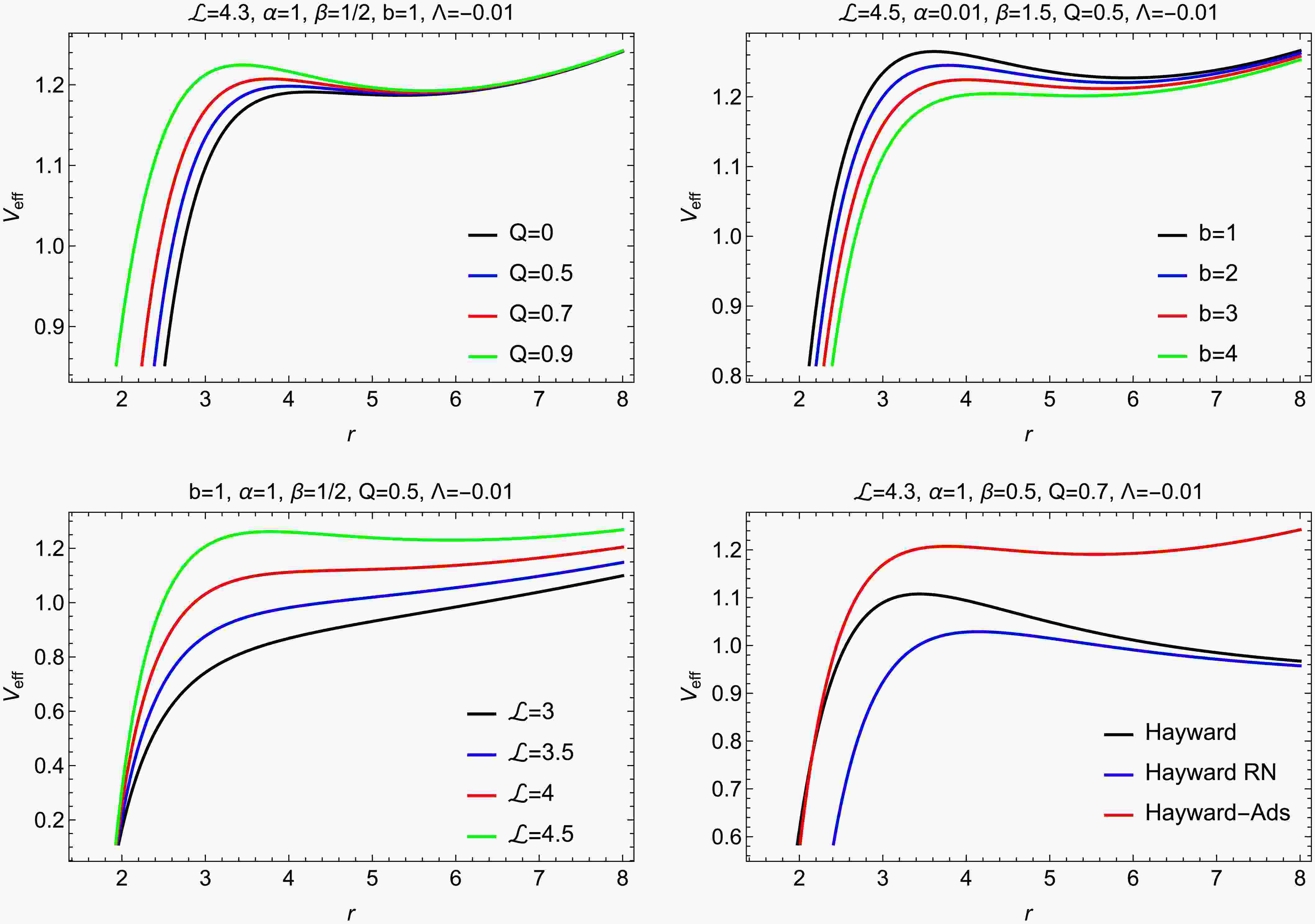
$V_{\rm eff}(r,\theta)$ , plays a crucial role in the study of test-particle dynamics. By analyzing the effective potential, we can avoid directly solving the complicated equations of motion, thereby gaining a more intuitive understanding of the particle's orbital characteristics. We investigate the behavior of the effective potential by varying the BH parameters, as shown in Fig. 1. The first row of the figure shows that the Hayward parameter Q and the BH parameter b have opposite effects on the stability of circular orbits: as Q increases, the maximum of the effective potential gradually approaches the event horizon, whereas as b increases, the maximum moves away from the event horizon. The second row shows the effect of different orbital angular momenta$ \mathcal{L} $ , indicating that greater angular momentum corresponds to more stable circular orbits. The lower panel further compares the effective-potential distributions for different BH models. It can be clearly seen that particle circular orbits around Hayward-AdS BHs are more stable than those around Hayward BHs and Hayward Reissner Nordström BHs.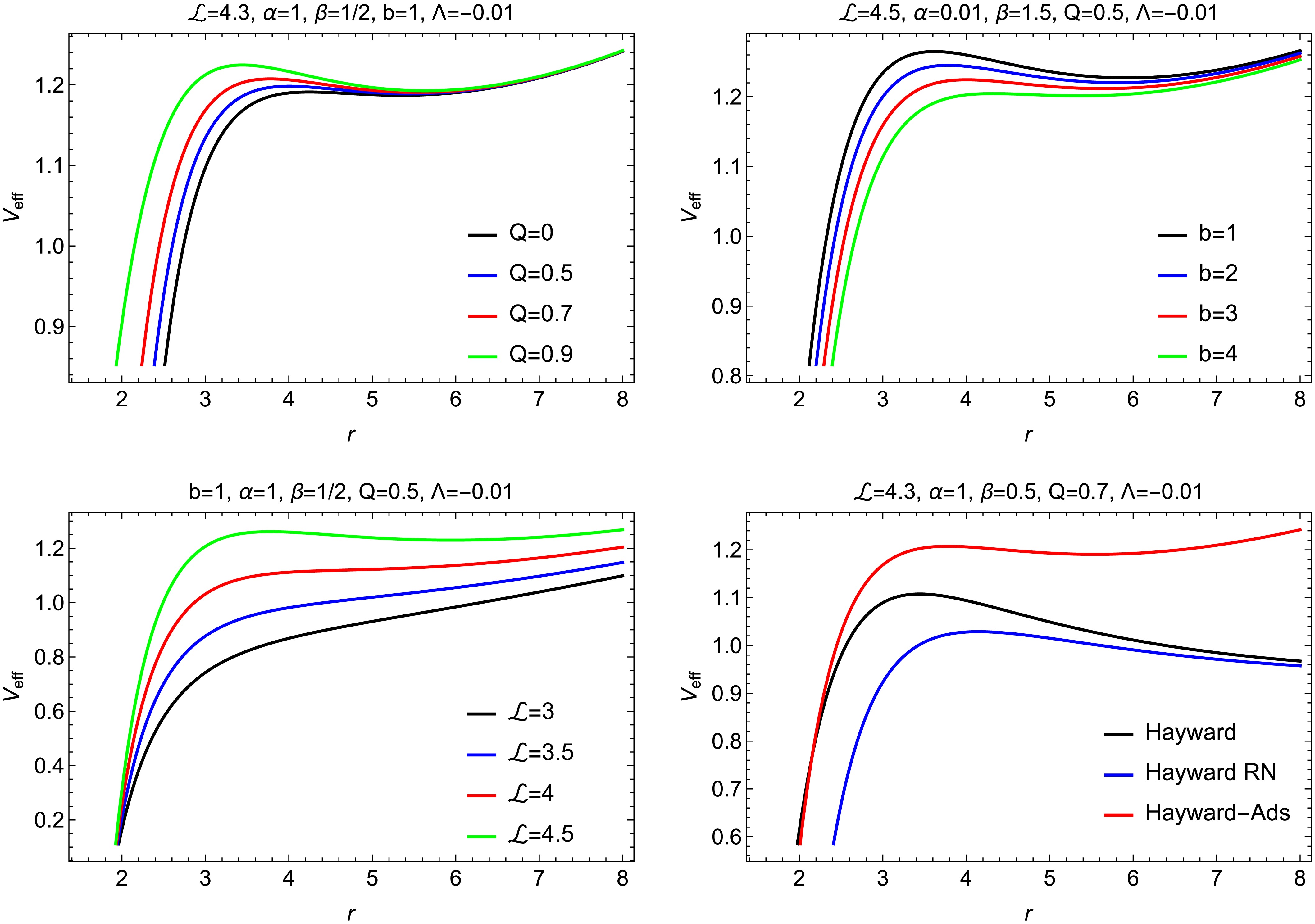
Figure 1. (color online) Plots of
$ V_{\rm eff}(r) $ versus r for different values of the relevant parameters, with$ M=1 $ .The circular orbits located in the equatorial plane
$ \theta=\pi/2 $ can be determined by the following conditions$ V_{\rm eff}(r) = {{\cal E}}^2, \quad \frac{{ \mathrm{d}} V_{\rm eff} (r)}{{ \mathrm{d}} r} = 0. $
(12) By analyzing Eq. (12), the conditions for circular orbits around the Hayward–AdS BH surrounded by a string fluid, as described by the metric (1), are obtained as
$ {{\cal L}} = \dfrac{r \sqrt{-\dfrac{\alpha \left(\dfrac{b}{r}\right)^{2/\beta }}{\beta -2}+\dfrac{r^2 \left(r^3-4 Q^2\right)}{\left(2 Q^2+r^3\right)^2}-\dfrac{\Lambda r^2}{3}}}{\sqrt{\dfrac{\alpha (\beta +1) \left(\dfrac{b}{r}\right)^{2/\beta }}{\beta -2}+\dfrac{4 Q^4+4 Q^2 r^3+(r-3) r^5}{\left(2 Q^2+r^3\right)^2}}}, $
(13) the corresponding energy for circular orbits can be expressed as follows:
$ {{\cal E}} = \dfrac{\dfrac{\alpha \beta \left(\dfrac{b}{r}\right)^{2/\beta }}{\beta -2}+r^2 \left(-\dfrac{\Lambda }{3}-\dfrac{2}{2 Q^2+r^3}\right)+1}{\sqrt{\dfrac{4 Q^4 \left(\alpha (\beta +1) \left(\dfrac{b}{r}\right)^{2/\beta }+\beta -2\right)+4 Q^2 r^3 \left(\alpha (\beta +1) \left(\dfrac{b}{r}\right)^{2/\beta }+\beta -2\right)+r^5 \left(r \left(\alpha (\beta +1) \left(\dfrac{b}{r}\right)^{2/\beta }+\beta -2\right)-3 \beta +6\right)}{(\beta -2) \left(2 Q^2+r^3\right)^2}}}. $
(14) As indicated in Fig. 2, the angular momentum of the test particles depends on the radial coordinate r in the spacetime of a Hayward-AdS BH surrounded by a fluid of strings. The plot is shown for several choices of BH parameters. It indicates that the smaller the Hayward parameter Q, the greater the angular momentum; conversely, the larger the Hayward parameter Q, the smaller the angular momentum. On the other hand, the angular momentum increases linearly with r. The parameter b also increases the angular momentum of the particles. The bottom panel compares the angular momentum in various BH geometries. The angular momentum of particles in the Hayward-AdS BH with a fluid of strings is greater than that in the pure Hayward and Hayward-RN cases.
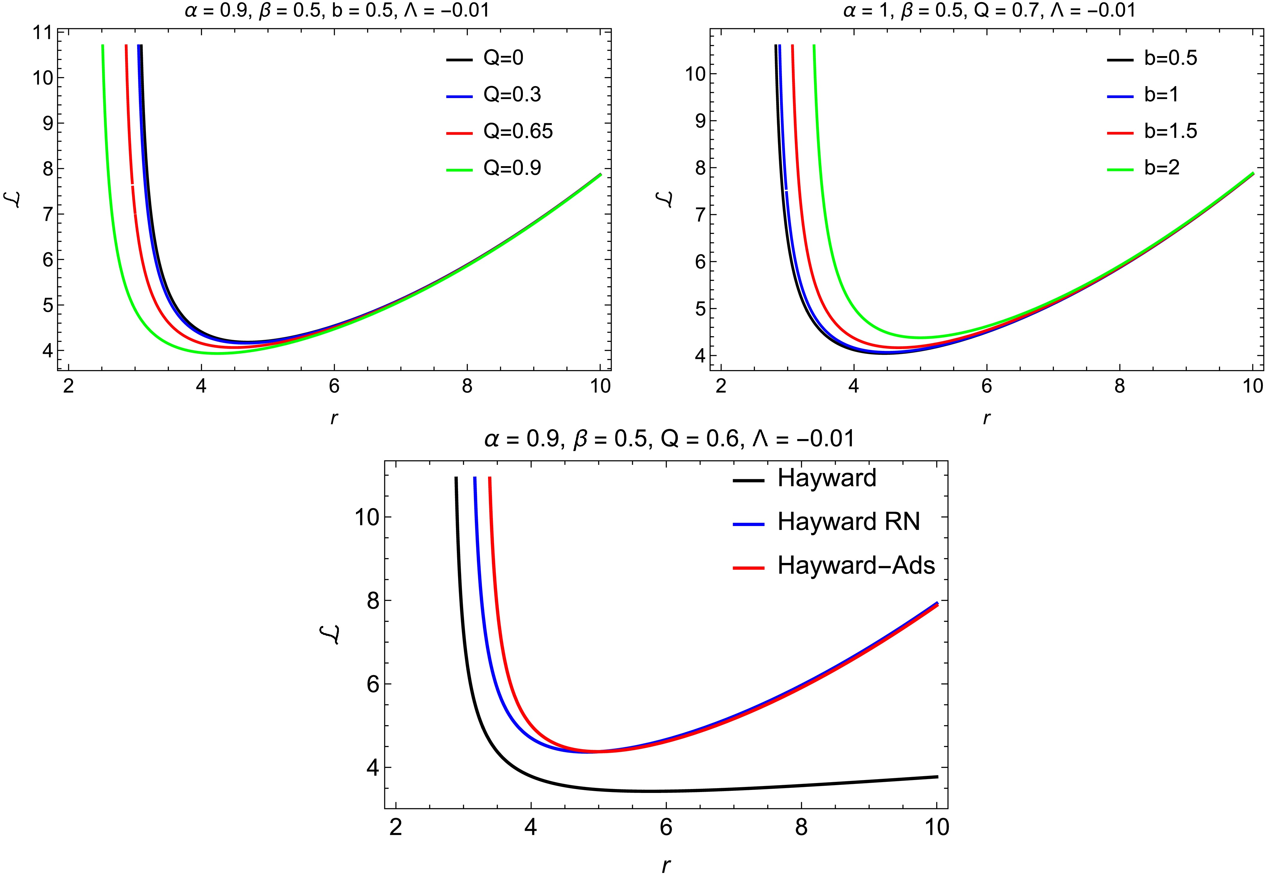
Figure 2. (color online) Plots of
$ {{\cal L}} $ versus r for different values of the relevant parameters, with$ M=1 $ .Figure 3 shows the behavior of the energy of the particles around the BH structure for different values of Q and b. The curves correspond to various sets of BH parameters. From the plot, we observe that the lower the Hayward parameter, the higher the particle energy, and vice versa. The effect of the parameter b is opposite; as b increases, the particle energy also increases. The lower panel compares the particle energy in various BH geometries. It demonstrates that particles in the Hayward-AdS BH with a fluid of strings have greater energy than those in the pure Hayward and Hayward-RN backgrounds.
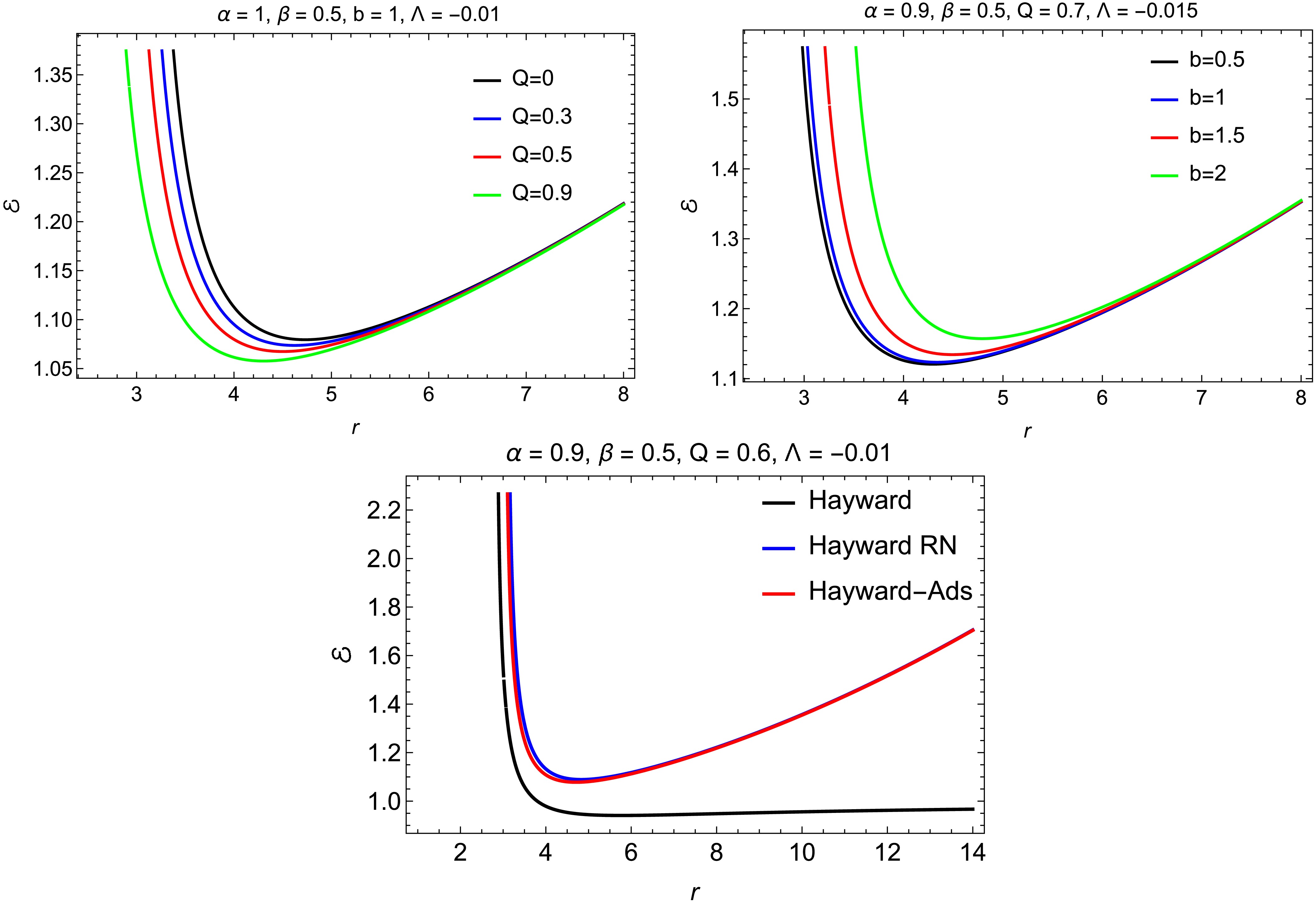
Figure 3. (color online) Plots of
$ {{\cal E}} $ versus r for different values of the relevant parameters, with$ M=1 $ .To clarify the origin of the enhanced orbital stability in the Hayward–AdS background, we emphasize that the stability of circular motion is determined by the structure of the effective potential
$ (V_{\text{eff}}(r)) $ , specifically by the presence and behavior of its extrema. Stable circular orbits correspond to well-defined local minima of the effective potential, whereas local maxima represent unstable configurations. As illustrated in Fig. 1, the Hayward–AdS BH develops deeper and more pronounced potential wells than the Hayward and Hayward–Reissner–Nordström cases, leading to clearer and more robust stable minima. This is why the stability of the Hayward–AdS orbits can clearly be seen from the plots: the potential well is both deeper and located farther from the event horizon, indicating that small perturbations are less likely to displace the particle from its orbit. The earlier discussion is now placed before the ISCO analysis to ensure continuity, and the subsequent ISCO plots in Fig. 4 further confirm that the Hayward–AdS geometry supports smaller and more stable circular-orbit radii than the other BH models.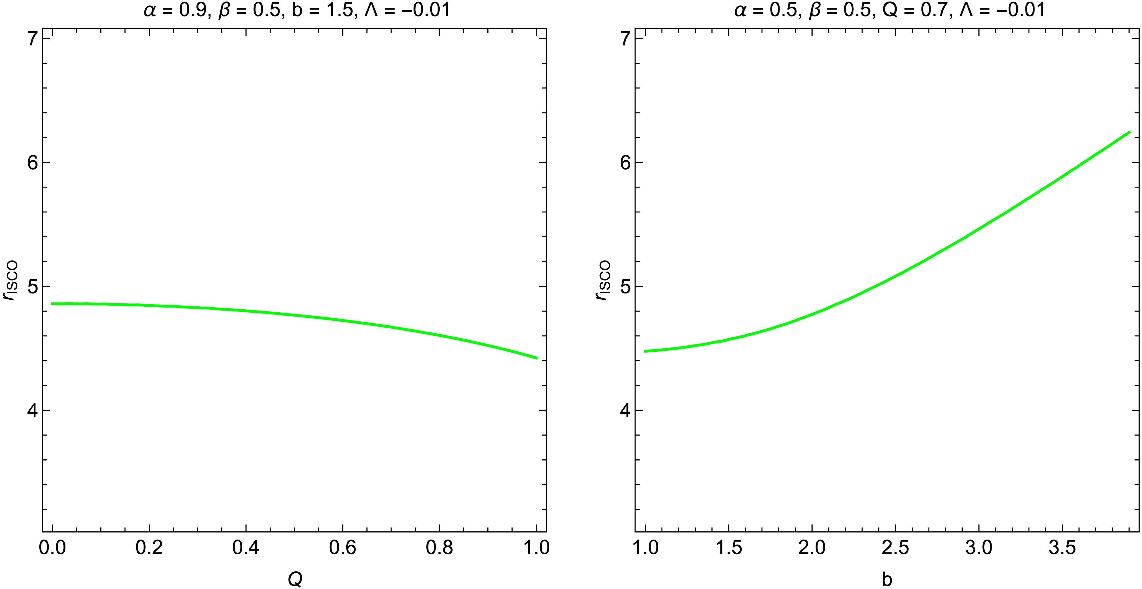
Figure 4. (color online) Plots of
$r_{\rm ISCO}$ versus Q and b for different values of the relevant parameters, with$ M=1 $ . -
The effective potential,
$V_{\rm eff}(r,\theta)$ , plays a crucial role in the study of test-particle dynamics. By analyzing the effective potential, we can avoid directly solving the complicated equations of motion, thereby gaining a more intuitive understanding of the particle's orbital characteristics. We investigate the behavior of the effective potential by varying the BH parameters, as shown in Fig. 1. The first row of the figure shows that the Hayward parameter Q and the BH parameter b have opposite effects on the stability of circular orbits: as Q increases, the maximum of the effective potential gradually approaches the event horizon, whereas as b increases, the maximum moves away from the event horizon. The second row shows the effect of different orbital angular momenta$ \mathcal{L} $ , indicating that greater angular momentum corresponds to more stable circular orbits. The lower panel further compares the effective-potential distributions for different BH models. It can be clearly seen that particle circular orbits around Hayward-AdS BHs are more stable than those around Hayward BHs and Hayward Reissner Nordström BHs.
Figure 1. (color online) Plots of
$ V_{\rm eff}(r) $ versus r for different values of the relevant parameters, with$ M=1 $ .The circular orbits located in the equatorial plane
$ \theta=\pi/2 $ can be determined by the following conditions$ V_{\rm eff}(r) = {{\cal E}}^2, \quad \frac{{ \mathrm{d}} V_{\rm eff} (r)}{{ \mathrm{d}} r} = 0. $
(12) By analyzing Eq. (12), the conditions for circular orbits around the Hayward–AdS BH surrounded by a string fluid, as described by the metric (1), are obtained as
$ {{\cal L}} = \dfrac{r \sqrt{-\dfrac{\alpha \left(\dfrac{b}{r}\right)^{2/\beta }}{\beta -2}+\dfrac{r^2 \left(r^3-4 Q^2\right)}{\left(2 Q^2+r^3\right)^2}-\dfrac{\Lambda r^2}{3}}}{\sqrt{\dfrac{\alpha (\beta +1) \left(\dfrac{b}{r}\right)^{2/\beta }}{\beta -2}+\dfrac{4 Q^4+4 Q^2 r^3+(r-3) r^5}{\left(2 Q^2+r^3\right)^2}}}, $
(13) the corresponding energy for circular orbits can be expressed as follows:
$ {{\cal E}} = \dfrac{\dfrac{\alpha \beta \left(\dfrac{b}{r}\right)^{2/\beta }}{\beta -2}+r^2 \left(-\dfrac{\Lambda }{3}-\dfrac{2}{2 Q^2+r^3}\right)+1}{\sqrt{\dfrac{4 Q^4 \left(\alpha (\beta +1) \left(\dfrac{b}{r}\right)^{2/\beta }+\beta -2\right)+4 Q^2 r^3 \left(\alpha (\beta +1) \left(\dfrac{b}{r}\right)^{2/\beta }+\beta -2\right)+r^5 \left(r \left(\alpha (\beta +1) \left(\dfrac{b}{r}\right)^{2/\beta }+\beta -2\right)-3 \beta +6\right)}{(\beta -2) \left(2 Q^2+r^3\right)^2}}}. $
(14) As indicated in Fig. 2, the angular momentum of the test particles depends on the radial coordinate r in the spacetime of a Hayward-AdS BH surrounded by a fluid of strings. The plot is shown for several choices of BH parameters. It indicates that the smaller the Hayward parameter Q, the greater the angular momentum; conversely, the larger the Hayward parameter Q, the smaller the angular momentum. On the other hand, the angular momentum increases linearly with r. The parameter b also increases the angular momentum of the particles. The bottom panel compares the angular momentum in various BH geometries. The angular momentum of particles in the Hayward-AdS BH with a fluid of strings is greater than that in the pure Hayward and Hayward-RN cases.
Figure 2. (color online) Plots of
$ {{\cal L}} $ versus r for different values of the relevant parameters, with$ M=1 $ .Figure 3 shows the behavior of the energy of the particles around the BH structure for different values of Q and b. The curves correspond to various sets of BH parameters. From the plot, we observe that the lower the Hayward parameter, the higher the particle energy, and vice versa. The effect of the parameter b is opposite; as b increases, the particle energy also increases. The lower panel compares the particle energy in various BH geometries. It demonstrates that particles in the Hayward-AdS BH with a fluid of strings have greater energy than those in the pure Hayward and Hayward-RN backgrounds.
Figure 3. (color online) Plots of
$ {{\cal E}} $ versus r for different values of the relevant parameters, with$ M=1 $ .To clarify the origin of the enhanced orbital stability in the Hayward–AdS background, we emphasize that the stability of circular motion is determined by the structure of the effective potential
$ (V_{\text{eff}}(r)) $ , specifically by the presence and behavior of its extrema. Stable circular orbits correspond to well-defined local minima of the effective potential, whereas local maxima represent unstable configurations. As illustrated in Fig. 1, the Hayward–AdS BH develops deeper and more pronounced potential wells than the Hayward and Hayward–Reissner–Nordström cases, leading to clearer and more robust stable minima. This is why the stability of the Hayward–AdS orbits can clearly be seen from the plots: the potential well is both deeper and located farther from the event horizon, indicating that small perturbations are less likely to displace the particle from its orbit. The earlier discussion is now placed before the ISCO analysis to ensure continuity, and the subsequent ISCO plots in Fig. 4 further confirm that the Hayward–AdS geometry supports smaller and more stable circular-orbit radii than the other BH models.
Figure 4. (color online) Plots of
$r_{\rm ISCO}$ versus Q and b for different values of the relevant parameters, with$ M=1 $ . -
The effective potential determines the maxima and minima associated with a particle's circular motion. Maxima correspond to unstable circular orbits, whereas minima indicate stable circular orbits. In the Newtonian regime, the innermost stable circular orbit (ISCO) for a given angular momentum is associated with the most negative value of the effective potential. The inclusion of additional effects, such as spin or other intrinsic particle properties, makes the potential profile more complicated, leading to shifts in orbital positions. In General Relativity, this complexity increases further. For example, in the Schwarzschild BH spacetime, the effective potential for a given angular momentum may exhibit two extrema, representing different orbital regimes.
In the present work, an accurate calculation of the angular momentum is necessary to determine the ISCO. It can be calculated using the following constraints:
$ \begin{split} & V_{\rm eff}(r) = {{\cal E}}^2, \quad \frac{{ \mathrm{d}} V_{\rm eff} (r)} {{ \mathrm{d}} \, r} = 0, \quad \frac{{ \mathrm{d}}^2 V_{\rm eff} (r)} {{ \mathrm{d}}\, r^2} = 0. \end{split} $
(15) The radii of the ISCOs can be determined from the equation
$ {\begin{split} & \dfrac{r \left(\dfrac{2 \alpha \left(\dfrac{b}{r}\right)^{2/\beta }}{(\beta -2) \beta r}+\dfrac{16 Q^2 r \left(r^3-Q^2\right)}{\left(2 Q^2+r^3\right)^3}-\dfrac{6 r^7}{\left(2 Q^2+r^3\right)^3}+\dfrac{5 r^4}{\left(2 Q^2+r^3\right)^2}-\dfrac{2 \Lambda r}{3}\right)}{2 \sqrt{\dfrac{\alpha (\beta +1) \left(\dfrac{b}{r}\right)^{2/\beta }}{\beta -2}+\dfrac{4 Q^4+4 Q^2 r^3+(r-3) r^5}{\left(2 Q^2+r^3\right)^2}} \sqrt{-\dfrac{\alpha \left(\dfrac{b}{r}\right)^{2/\beta }}{\beta -2}+ \dfrac{r^2 \left(r^3-4 Q^2\right)}{\left(2 Q^2+r^3\right)^2}-\dfrac{\Lambda r^2}{3}}} \\+&\dfrac{\sqrt{-\dfrac{\alpha \left(\dfrac{b}{r}\right)^{2/\beta }}{\beta -2}+\dfrac{r^2 \left(r^3-4 Q^2\right)}{\left(2 Q^2+r^3\right)^2}-\dfrac{\Lambda r^2}{3}}}{\sqrt{\dfrac{\alpha (\beta +1) \left(\dfrac{b}{r}\right)^{2/\beta }}{\beta -2}+\dfrac{4 Q^4+4 Q^2 r^3+(r-3) r^5}{\left(2 Q^2+r^3\right)^2}}} \\ + & \dfrac{r \left(-\dfrac{2 \alpha (\beta +1) \left(\dfrac{b}{r}\right)^{2/\beta }}{(\beta -2) \beta r}+\dfrac{3 \left(4 Q^2 r^2+(2 r-5) r^4\right)}{\left(2 Q^2+r^3\right)^2}-\dfrac{6 r^2 \left(4 Q^4+4 Q^2 r^3+(r-3) r^5\right)}{\left(2 Q^2+r^3\right)^3}\right) \sqrt{-\dfrac{\alpha \left(\dfrac{b}{r}\right)^{2/\beta }}{\beta -2}+\dfrac{r^2 \left(r^3-4 Q^2\right)}{\left(2 Q^2+r^3\right)^2}-\dfrac{\Lambda r^2}{3}}}{2 \left(\dfrac{\alpha (\beta +1) \left(\dfrac{b}{r}\right)^{2/\beta }}{\beta -2}+\dfrac{4 Q^4+4 Q^2 r^3+(r-3) r^5}{\left(2 Q^2+r^3\right)^2}\right)^{3/2}} = 0. \end{split}} $
(16) In Fig. 4, we examine the equatorial ISCOs and their dependence on the BH parameters Q and b. The graphical analysis shows that, for a fixed value of the string cloud parameter b, the ISCO radii decrease as Q increases. Likewise, as b increases, the ISCO radii decrease.
-
The effective potential determines the maxima and minima associated with a particle's circular motion. Maxima correspond to unstable circular orbits, whereas minima indicate stable circular orbits. In the Newtonian regime, the innermost stable circular orbit (ISCO) for a given angular momentum is associated with the most negative value of the effective potential. The inclusion of additional effects, such as spin or other intrinsic particle properties, makes the potential profile more complicated, leading to shifts in orbital positions. In General Relativity, this complexity increases further. For example, in the Schwarzschild BH spacetime, the effective potential for a given angular momentum may exhibit two extrema, representing different orbital regimes.
In the present work, an accurate calculation of the angular momentum is necessary to determine the ISCO. It can be calculated using the following constraints:
$ \begin{split} & V_{\rm eff}(r) = {{\cal E}}^2, \quad \frac{{ \mathrm{d}} V_{\rm eff} (r)} {{ \mathrm{d}} \, r} = 0, \quad \frac{{ \mathrm{d}}^2 V_{\rm eff} (r)} {{ \mathrm{d}}\, r^2} = 0. \end{split} $
(15) The radii of the ISCOs can be determined from the equation
$ {\begin{split} & \dfrac{r \left(\dfrac{2 \alpha \left(\dfrac{b}{r}\right)^{2/\beta }}{(\beta -2) \beta r}+\dfrac{16 Q^2 r \left(r^3-Q^2\right)}{\left(2 Q^2+r^3\right)^3}-\dfrac{6 r^7}{\left(2 Q^2+r^3\right)^3}+\dfrac{5 r^4}{\left(2 Q^2+r^3\right)^2}-\dfrac{2 \Lambda r}{3}\right)}{2 \sqrt{\dfrac{\alpha (\beta +1) \left(\dfrac{b}{r}\right)^{2/\beta }}{\beta -2}+\dfrac{4 Q^4+4 Q^2 r^3+(r-3) r^5}{\left(2 Q^2+r^3\right)^2}} \sqrt{-\dfrac{\alpha \left(\dfrac{b}{r}\right)^{2/\beta }}{\beta -2}+ \dfrac{r^2 \left(r^3-4 Q^2\right)}{\left(2 Q^2+r^3\right)^2}-\dfrac{\Lambda r^2}{3}}} \\+&\dfrac{\sqrt{-\dfrac{\alpha \left(\dfrac{b}{r}\right)^{2/\beta }}{\beta -2}+\dfrac{r^2 \left(r^3-4 Q^2\right)}{\left(2 Q^2+r^3\right)^2}-\dfrac{\Lambda r^2}{3}}}{\sqrt{\dfrac{\alpha (\beta +1) \left(\dfrac{b}{r}\right)^{2/\beta }}{\beta -2}+\dfrac{4 Q^4+4 Q^2 r^3+(r-3) r^5}{\left(2 Q^2+r^3\right)^2}}} \\ + & \dfrac{r \left(-\dfrac{2 \alpha (\beta +1) \left(\dfrac{b}{r}\right)^{2/\beta }}{(\beta -2) \beta r}+\dfrac{3 \left(4 Q^2 r^2+(2 r-5) r^4\right)}{\left(2 Q^2+r^3\right)^2}-\dfrac{6 r^2 \left(4 Q^4+4 Q^2 r^3+(r-3) r^5\right)}{\left(2 Q^2+r^3\right)^3}\right) \sqrt{-\dfrac{\alpha \left(\dfrac{b}{r}\right)^{2/\beta }}{\beta -2}+\dfrac{r^2 \left(r^3-4 Q^2\right)}{\left(2 Q^2+r^3\right)^2}-\dfrac{\Lambda r^2}{3}}}{2 \left(\dfrac{\alpha (\beta +1) \left(\dfrac{b}{r}\right)^{2/\beta }}{\beta -2}+\dfrac{4 Q^4+4 Q^2 r^3+(r-3) r^5}{\left(2 Q^2+r^3\right)^2}\right)^{3/2}} = 0. \end{split}} $
(16) In Fig. 4, we examine the equatorial ISCOs and their dependence on the BH parameters Q and b. The graphical analysis shows that, for a fixed value of the string cloud parameter b, the ISCO radii decrease as Q increases. Likewise, as b increases, the ISCO radii decrease.
-
The trajectory of a particle is determined by the effective force acting on it, which indicates whether the particle is attracted toward the BH or repelled from it. Here, we analyze the motion of a particle in the spacetime of a Hayward–AdS BH surrounded by a string fluid, in which the gravity of the BH may be either attractive or repulsive. Using Eq. (11), the effective force can be defined as [75, 76]:
$ \begin{split} F =& - \frac{1}{2}\frac{{\rm d} V_{\rm eff}}{{\rm d}r},\\ =& {{\cal L}}^2 \left(\dfrac{\alpha (\beta +1) \left(\dfrac{b}{r}\right)^{2/\beta }+\beta -2}{(\beta -2) r^3}-\dfrac{3 r^2}{\left(2 Q^2+r^3\right)^2}\right)\\ &+\dfrac{\alpha \left(\dfrac{b}{r}\right)^{2/\beta }}{(\beta -2) r}+\dfrac{2 r}{2 Q^2+r^3}-\dfrac{3 r^4}{\left(2 Q^2+r^3\right)^2}+\dfrac{\Lambda r}{3}. \end{split} $
(17) Figure 5 illustrates the radial profile of the effective force for several choices of the black-hole parameters. Since all curves satisfy the condition
$ F(r)\leq 0 $ , the force remains attractive throughout the entire parameter space considered. Consequently, variations in the spacetime parameters are manifested primarily through changes in the magnitude of the effective force, rather than through any change in its sign. In particular, smaller values of the Hayward parameter Q produce more negative values of$ F(r) $ , corresponding to a stronger inward gravitational attraction, whereas increasing Q systematically reduces the force magnitude. An analogous behavior is observed for the parameter b: increasing b shifts the effective force toward less negative values, indicating a weaker attractive interaction, while decreasing b enhances the gravitational pull.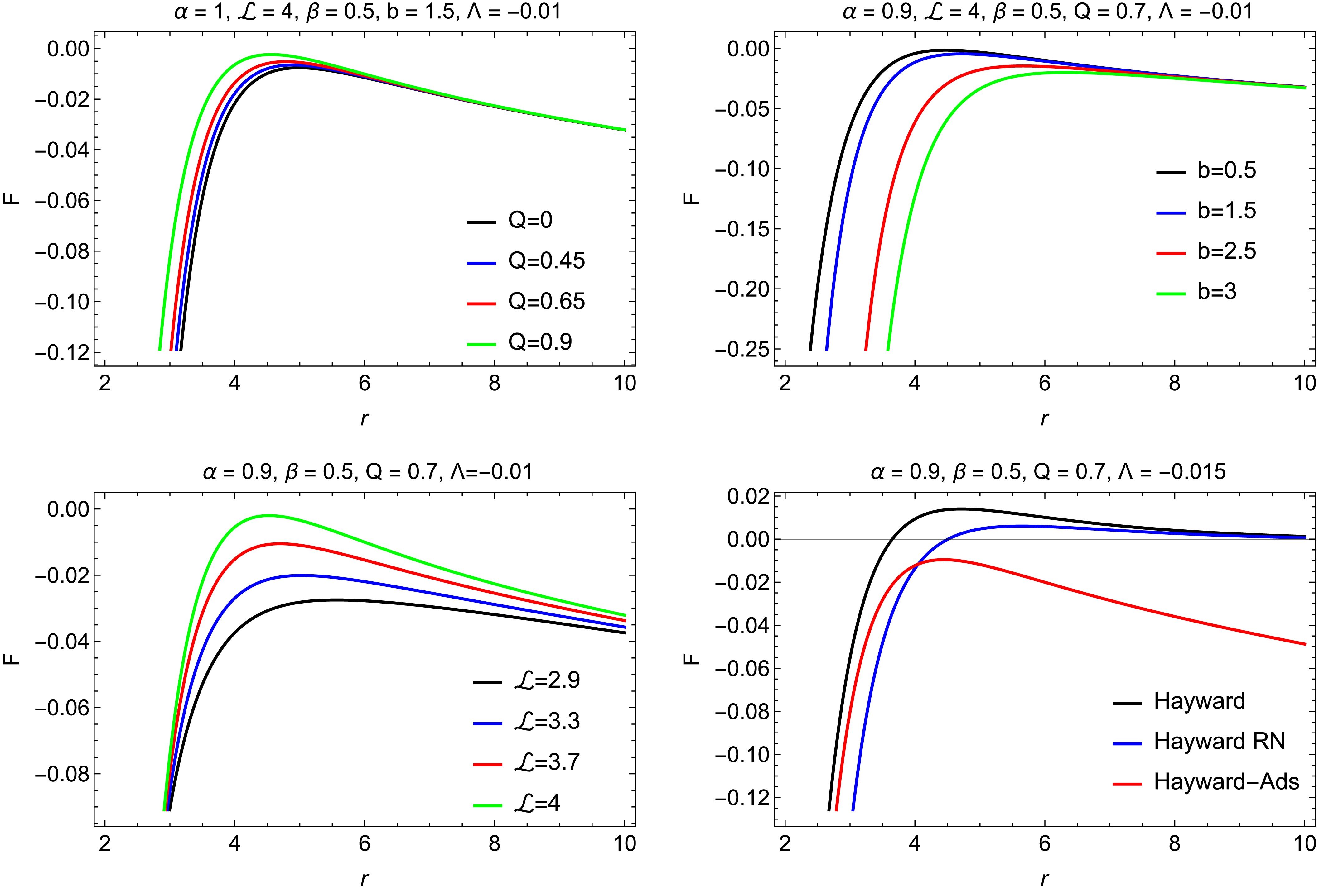
Figure 5. (color online) Plots of F versus r for different values of the relevant parameters, with
$ M=1 $ . -
The trajectory of a particle is determined by the effective force acting on it, which indicates whether the particle is attracted toward the BH or repelled from it. Here, we analyze the motion of a particle in the spacetime of a Hayward–AdS BH surrounded by a string fluid, in which the gravity of the BH may be either attractive or repulsive. Using Eq. (11), the effective force can be defined as [75, 76]:
$ \begin{split} F =& - \frac{1}{2}\frac{{\rm d} V_{\rm eff}}{{\rm d}r},\\ =& {{\cal L}}^2 \left(\dfrac{\alpha (\beta +1) \left(\dfrac{b}{r}\right)^{2/\beta }+\beta -2}{(\beta -2) r^3}-\dfrac{3 r^2}{\left(2 Q^2+r^3\right)^2}\right)\\ &+\dfrac{\alpha \left(\dfrac{b}{r}\right)^{2/\beta }}{(\beta -2) r}+\dfrac{2 r}{2 Q^2+r^3}-\dfrac{3 r^4}{\left(2 Q^2+r^3\right)^2}+\dfrac{\Lambda r}{3}. \end{split} $
(17) Figure 5 illustrates the radial profile of the effective force for several choices of the black-hole parameters. Since all curves satisfy the condition
$ F(r)\leq 0 $ , the force remains attractive throughout the entire parameter space considered. Consequently, variations in the spacetime parameters are manifested primarily through changes in the magnitude of the effective force, rather than through any change in its sign. In particular, smaller values of the Hayward parameter Q produce more negative values of$ F(r) $ , corresponding to a stronger inward gravitational attraction, whereas increasing Q systematically reduces the force magnitude. An analogous behavior is observed for the parameter b: increasing b shifts the effective force toward less negative values, indicating a weaker attractive interaction, while decreasing b enhances the gravitational pull.
Figure 5. (color online) Plots of F versus r for different values of the relevant parameters, with
$ M=1 $ . -
We study small deviations in the equations of motion of neutral particles in circular orbits. Specifically, we consider a small perturbation of a test particle from its equilibrium position in the equatorial plane, which gives rise to so-called epicyclic motion, i.e., small linear oscillations about a stable circular orbit.
-
We study small deviations in the equations of motion of neutral particles in circular orbits. Specifically, we consider a small perturbation of a test particle from its equilibrium position in the equatorial plane, which gives rise to so-called epicyclic motion, i.e., small linear oscillations about a stable circular orbit.
-
The frequencies associated with the harmonic oscillations, as measured by a local observer, can be expressed as follows [77, 78]:
$ \omega_{r}^{2} = -\frac{1}{2}\frac{\partial^{2} V_{\rm eff}(r, \theta)}{\partial r^{2}}, $
(18) $ \omega_{\theta}^{2} = \frac{1}{2}\frac{g_{rr} (r, \theta)}{r^2} \frac{\partial^{2} V_{\rm eff}(r, \theta)}{\partial \theta^{2}}, $
(19) $ \omega_\phi = \frac{{ \mathrm{d}} \phi}{{ \mathrm{d}} \tau}. $
(20) The corresponding frequencies of neutral test-particle motion around the Hayward-Ads BH are given by
$ \begin{split} \omega_{r}^{2} =& \dfrac{1}{4 \sqrt{\left(\dfrac{L^2}{r^2}+1\right) \left(\dfrac{\alpha \beta \left(\dfrac{b}{r}\right)^{2/\beta }}{\beta -2}+r^2 \left(-\dfrac{\Lambda }{3}-\dfrac{2}{\left(Q^2+r^2\right)^{3/2}}\right)+1\right)}}\Bigg[L^2 \Bigg[\dfrac{2 \left(\dfrac{\alpha \left(3 \beta ^2+5 \beta +2\right) \left(\dfrac{b}{r}\right)^{2/\beta }}{(\beta -2) \beta }+3\right)}{r^4}-\dfrac{30 r^2}{\left(Q^2+r^2\right)^{7/2}}\\ &+ \dfrac{6}{\left(Q^2+r^2\right)^{5/2}} \Bigg]+\dfrac{2 \alpha (\beta +2) \left(\dfrac{b}{r}\right)^{2/\beta }}{(\beta -2) \beta r^2}- \dfrac{2 \Lambda }{3}-\dfrac{4}{\left(Q^2+r^2\right)^{3/2}}+\dfrac{30 r^2}{\left(Q^2+r^2\right)^{5/2}}-\dfrac{30 r^4}{\left(Q^2+r^2\right)^{7/2}}\Bigg]\\ &- \dfrac{\left(L^2 \left(\dfrac{6 r}{\left(Q^2+r^2\right)^{5/2}}-\dfrac{2 \left(\alpha (\beta +1) \left(\dfrac{b}{r}\right)^{2/\beta }+\beta -2\right)}{(\beta -2) r^3}\right)-\dfrac{2 \alpha \left(\dfrac{b}{r}\right)^{2/\beta }}{(\beta -2) r}-\dfrac{4 r}{\left(Q^2+r^2\right)^{3/2}}+\dfrac{6 r^3}{\left(Q^2+r^2\right)^{5/2}}-\dfrac{2 \Lambda r}{3}\right)^2}{8 \left(\left(\dfrac{L^2}{r^2}+1\right) \left(\dfrac{\alpha \beta \left(\dfrac{b}{r}\right)^{2/\beta }}{\beta -2}+r^2 \left(-\dfrac{\Lambda }{3}-\dfrac{2}{\left(Q^2+r^2\right)^{3/2}}\right)+1\right)\right)^{3/2}}, \end{split} $
(21) $ \omega_{\theta}^{2} = \dfrac{-\dfrac{\alpha \left(\dfrac{b}{r}\right)^{2/\beta }}{\beta -2}+\dfrac{r^2 \left(r^3-4 Q^2\right)}{\left(2 Q^2+r^3\right)^2}-\dfrac{\Lambda r^2}{3}}{r^2 \left(\dfrac{\alpha (\beta +1) \left(\dfrac{b}{r}\right)^{2/\beta }}{\beta -2}+\dfrac{4 Q^4+4 Q^2 r^3+(r-3) r^5}{\left(2 Q^2+r^3\right)^2}\right)}, $
(22) $ {\omega^2_\phi = \dfrac{-\dfrac{\alpha \left(\dfrac{b}{r}\right)^{2/\beta }}{\beta -2}+\dfrac{r^2 \left(r^3-4 Q^2\right)}{\left(2 Q^2+r^3\right)^2}-\dfrac{\Lambda r^2}{3}}{r^2 \left(\dfrac{\alpha (\beta +1) \left(\dfrac{b}{r}\right)^{2/\beta }}{\beta -2}+\dfrac{4 Q^4+4 Q^2 r^3+(r-3) r^5}{\left(2 Q^2+r^3\right)^2}\right)}.} $
(23) -
The frequencies associated with the harmonic oscillations, as measured by a local observer, can be expressed as follows [77, 78]:
$ \omega_{r}^{2} = -\frac{1}{2}\frac{\partial^{2} V_{\rm eff}(r, \theta)}{\partial r^{2}}, $
(18) $ \omega_{\theta}^{2} = \frac{1}{2}\frac{g_{rr} (r, \theta)}{r^2} \frac{\partial^{2} V_{\rm eff}(r, \theta)}{\partial \theta^{2}}, $
(19) $ \omega_\phi = \frac{{ \mathrm{d}} \phi}{{ \mathrm{d}} \tau}. $
(20) The corresponding frequencies of neutral test-particle motion around the Hayward-Ads BH are given by
$ \begin{split} \omega_{r}^{2} =& \dfrac{1}{4 \sqrt{\left(\dfrac{L^2}{r^2}+1\right) \left(\dfrac{\alpha \beta \left(\dfrac{b}{r}\right)^{2/\beta }}{\beta -2}+r^2 \left(-\dfrac{\Lambda }{3}-\dfrac{2}{\left(Q^2+r^2\right)^{3/2}}\right)+1\right)}}\Bigg[L^2 \Bigg[\dfrac{2 \left(\dfrac{\alpha \left(3 \beta ^2+5 \beta +2\right) \left(\dfrac{b}{r}\right)^{2/\beta }}{(\beta -2) \beta }+3\right)}{r^4}-\dfrac{30 r^2}{\left(Q^2+r^2\right)^{7/2}}\\ &+ \dfrac{6}{\left(Q^2+r^2\right)^{5/2}} \Bigg]+\dfrac{2 \alpha (\beta +2) \left(\dfrac{b}{r}\right)^{2/\beta }}{(\beta -2) \beta r^2}- \dfrac{2 \Lambda }{3}-\dfrac{4}{\left(Q^2+r^2\right)^{3/2}}+\dfrac{30 r^2}{\left(Q^2+r^2\right)^{5/2}}-\dfrac{30 r^4}{\left(Q^2+r^2\right)^{7/2}}\Bigg]\\ &- \dfrac{\left(L^2 \left(\dfrac{6 r}{\left(Q^2+r^2\right)^{5/2}}-\dfrac{2 \left(\alpha (\beta +1) \left(\dfrac{b}{r}\right)^{2/\beta }+\beta -2\right)}{(\beta -2) r^3}\right)-\dfrac{2 \alpha \left(\dfrac{b}{r}\right)^{2/\beta }}{(\beta -2) r}-\dfrac{4 r}{\left(Q^2+r^2\right)^{3/2}}+\dfrac{6 r^3}{\left(Q^2+r^2\right)^{5/2}}-\dfrac{2 \Lambda r}{3}\right)^2}{8 \left(\left(\dfrac{L^2}{r^2}+1\right) \left(\dfrac{\alpha \beta \left(\dfrac{b}{r}\right)^{2/\beta }}{\beta -2}+r^2 \left(-\dfrac{\Lambda }{3}-\dfrac{2}{\left(Q^2+r^2\right)^{3/2}}\right)+1\right)\right)^{3/2}}, \end{split} $
(21) $ \omega_{\theta}^{2} = \dfrac{-\dfrac{\alpha \left(\dfrac{b}{r}\right)^{2/\beta }}{\beta -2}+\dfrac{r^2 \left(r^3-4 Q^2\right)}{\left(2 Q^2+r^3\right)^2}-\dfrac{\Lambda r^2}{3}}{r^2 \left(\dfrac{\alpha (\beta +1) \left(\dfrac{b}{r}\right)^{2/\beta }}{\beta -2}+\dfrac{4 Q^4+4 Q^2 r^3+(r-3) r^5}{\left(2 Q^2+r^3\right)^2}\right)}, $
(22) $ {\omega^2_\phi = \dfrac{-\dfrac{\alpha \left(\dfrac{b}{r}\right)^{2/\beta }}{\beta -2}+\dfrac{r^2 \left(r^3-4 Q^2\right)}{\left(2 Q^2+r^3\right)^2}-\dfrac{\Lambda r^2}{3}}{r^2 \left(\dfrac{\alpha (\beta +1) \left(\dfrac{b}{r}\right)^{2/\beta }}{\beta -2}+\dfrac{4 Q^4+4 Q^2 r^3+(r-3) r^5}{\left(2 Q^2+r^3\right)^2}\right)}.} $
(23) -
In addition, it is worth noting that the angular frequencies
$ \omega_\beta $ , with$ \beta\in\{r,\theta,\phi\} $ , are presented in Eqs. (23)–(24). For distant observers, we get$ \Omega_{i} = \omega_{\beta} \frac{{ \mathrm{d}} T}{{ \mathrm{d}}\tau}, $
(24) where
$ \dfrac{{ \mathrm{d}} T}{{ \mathrm{d}}\tau} $ has already been defined in Eq. (7). For neutral particles, one obtains [77, 78]$ \nu_{i}=\frac{1}{2\pi}\frac{c^{3}}{GM} \, \Omega_{i}[{ {\rm{Hz}}}], $
(25) In the above,
$ i\in\{r,\theta,\phi\} $ , and$ \Omega_{r} $ ,$ \Omega_{\theta} $ , and$ \Omega_{\phi} $ denote the dimensionless radial, latitudinal, and axial angular frequencies. as measured from afar, we have$ \begin{split} \Omega_{r}^{2} =&-\frac{1}{\Omega_1}\Big[3 \Big[16 Q^6 \Big[\alpha (\beta -2) \left(\frac{b}{r}\right)^{2/\beta } \left(2 \beta ^2 \Lambda r^2+3 \beta \left(\Lambda r^2+1\right)+\Lambda r^2-3\right)+3 \alpha ^2 \beta (\beta +1) \left(\frac{b}{r}\right)^{4/\beta }\\ & + 2 (\beta -2)^2 \beta \Lambda r^2\Big]+24 Q^4 r^2 \Big[\alpha (\beta -2) \left(\frac{b}{r}\right)^{2/\beta } \left(4 \beta ^2+6 \beta +\left(2 \beta ^2+3 \beta +1\right) \Lambda r^3+3 (\beta -1) r+2\right)\\ & + 3 \alpha ^2 \beta (\beta +1) r \left(\frac{b}{r}\right)^{4/\beta }+2 (\beta -2)^2 \beta \left(\Lambda r^3+2\right)\Big]+6 Q^2 r^5 \Big[\alpha (\beta -2) \left(\frac{b}{r}\right)^{2/\beta } \Big[-11 \beta ^2\\ & + 2 \left(2 \beta ^2+3 \beta +1\right) \Lambda r^3+6 (\beta -1) r+8\Big]+6 \alpha ^2 \beta (\beta +1) r \left(\frac{b}{r}\right)^{4/\beta }+(\beta -2)^2 \beta \left(4 \Lambda r^3+\Lambda r^2-11\right)\Big]\\ & + r^7 \Big[2 (\beta -2) \Lambda r^4 \left(\alpha \left(2 \beta ^2+3 \beta +1\right) \left(\frac{b}{r}\right)^{2/\beta }+2 (\beta -2) \beta \right)+6 \alpha r^2 \left(\frac{b}{r}\right)^{2/\beta } \Big[\beta ^2 \left(\alpha \left(\frac{b}{r}\right)^{2/\beta }+1\right)\\ & + \beta \left(\alpha \left(\frac{b}{r}\right)^{2/\beta }-3\right)+2\Big]-3 (\beta -2) r \left(\alpha \left(\beta ^2+12 \beta -4\right) \left(\frac{b}{r}\right)^{2/\beta }+(\beta -2) \beta \right)+18 (\beta -2)^2 \beta \\ & - 15 (\beta -2)^2 \beta \Lambda r^3\Big]\Big]\Big] , \end{split} $
(26) $ \begin{split} \Omega_{\theta}^{2} = &\frac{1}{3 (\beta -2) \left(2 Q^2 r+r^4\right)^2} \left(-4 Q^4 \left(3 \alpha \left(\frac{b}{r}\right)^{2/\beta }+(\beta -2) \Lambda r^2\right) -4 Q^2 r^2 \left(3 \alpha r \left(\frac{b}{r}\right)^{2/\beta }+3 (\beta -2)+(\beta -2) \Lambda r^3\right)\right. \\ & \left.- \left(r^5 \left(3 \alpha r \left(\frac{b}{r}\right)^{2/\beta }-3 \beta +(\beta -2) \Lambda r^3+6\right)\right)\right) , \end{split} $
(27) $ \begin{split} \Omega_\phi^2 =& \frac{1}{3 (\beta -2) \left(2 Q^2 r+r^4\right)^2} \left(-4 Q^4 \left(3 \alpha \left(\frac{b}{r}\right)^{2/\beta }+(\beta -2) \Lambda r^2\right)-4 Q^2 r^2 \left(3 \alpha r \left(\frac{b}{r}\right)^{2/\beta }+3 (\beta -2)+(\beta -2) \Lambda r^3\right)\right. \\ & \left.- \left(r^5 \left(3 \alpha r \left(\frac{b}{r}\right)^{2/\beta }-3 \beta +(\beta -2) \Lambda r^3+6\right)\right)\right), \end{split} $
(28) where,
$ \begin{split} \Omega_1=&\beta \left(2 Q^2+r^3\right) \Big[2 Q^2 r \Big[\beta \Big[-3 \alpha \left(\frac{b}{r}\right)^{2/\beta }+\Lambda r^2-3\Big]\\ &-2 \Lambda r^2+6\Big]+r^3 \Big[-3 r \Big[\alpha \beta \left(\frac{b}{r}\right)^{2/\beta }+\beta -2\Big]\\ &+ 6 (\beta -2)+(\beta -2) \Lambda r^3\Big]\Big]^2. \end{split} $
The precise relationships between the fundamental frequencies and the oscillation modes can be expressed in physical units. In particular, the dimensionless angular frequencies can be rescaled by the characteristic gravitational factor
$c^{3}/(GM)$ , where M is the mass parameter of the black hole (BH) model under consideration. The exact expressions for the fundamental frequencies are obtained by substituting Eqs. (22)–(24) into Eq. (26). By constraining the motion to the equatorial plane,$\theta = \pi/2$ , in accordance with the symmetry of the spacetime metric, one finds that the azimuthal and polar epicyclic frequencies become identical,$\nu_{\phi} = \nu_{\theta}$ .Figure 6 demonstrates the radial dependence of the frequencies of small harmonic oscillations of neutral particles about a Hayward BH in the AdS scenario, as observed by a distant observer in the background of a string fluid. The radial frequencies are represented by black curves, while the magenta curves denote the orbital frequencies around the BH under consideration. An increase in the value of b causes the profiles to shift outward, away from the BH horizon. In contrast, increasing the Hayward parameter Q shifts the profiles inward, toward the center and closer to the horizon. It is evident from all the plots that the radial and orbital frequencies follow nearly the same trend. Noticeable differences arise only at very small scales and depend on the specific values of the parameters b and Q.
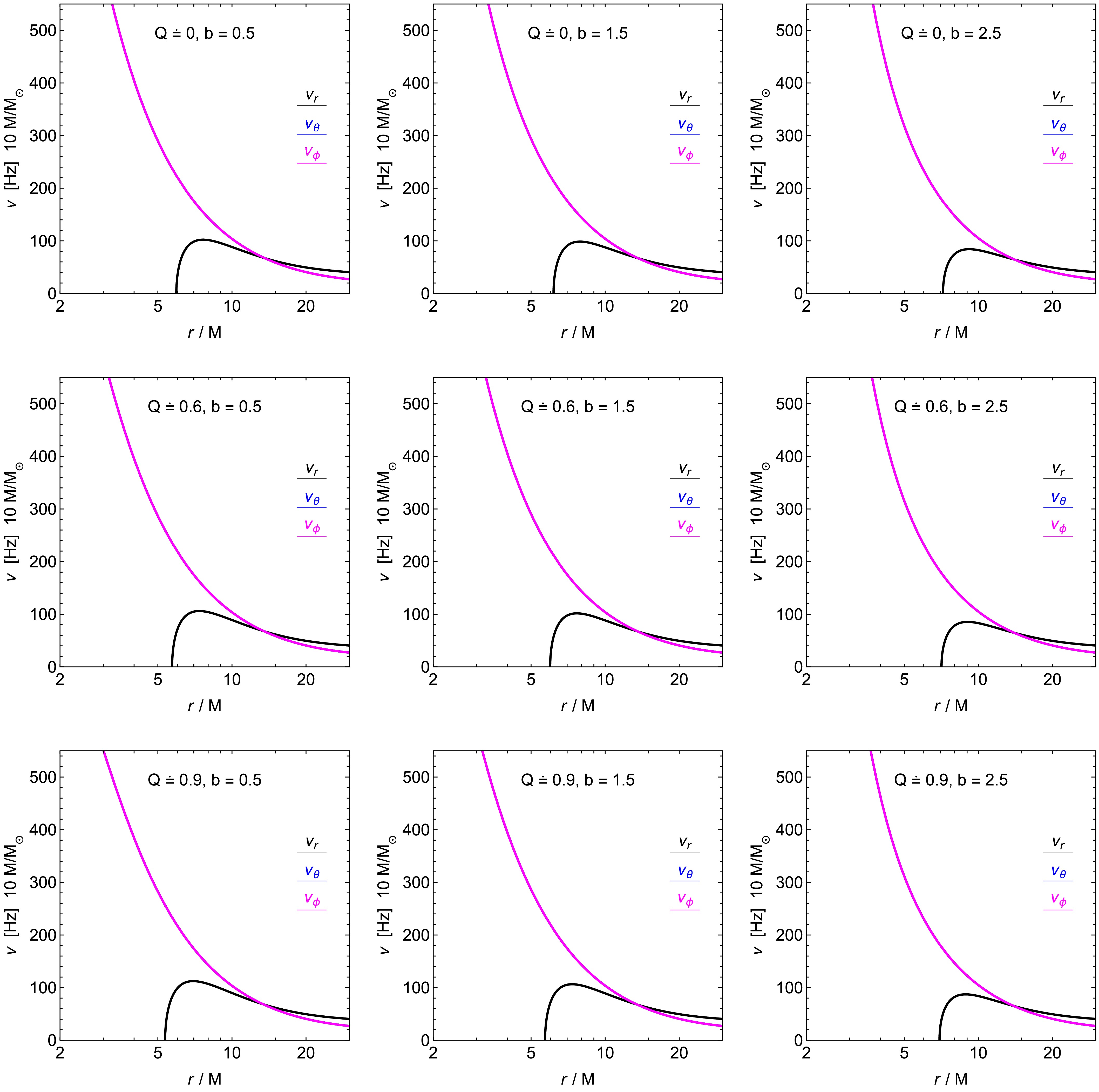
Figure 6. (color online) Frequencies of particles in the background of a Hayward-AdS BH within a string fluid, for varying values of the underlying model parameters.
-
In addition, it is worth noting that the angular frequencies
$ \omega_\beta $ , with$ \beta\in\{r,\theta,\phi\} $ , are presented in Eqs. (23)–(24). For distant observers, we get$ \Omega_{i} = \omega_{\beta} \frac{{ \mathrm{d}} T}{{ \mathrm{d}}\tau}, $
(24) where
$ \dfrac{{ \mathrm{d}} T}{{ \mathrm{d}}\tau} $ has already been defined in Eq. (7). For neutral particles, one obtains [77, 78]$ \nu_{i}=\frac{1}{2\pi}\frac{c^{3}}{GM} \, \Omega_{i}[{ {\rm{Hz}}}], $
(25) In the above,
$ i\in\{r,\theta,\phi\} $ , and$ \Omega_{r} $ ,$ \Omega_{\theta} $ , and$ \Omega_{\phi} $ denote the dimensionless radial, latitudinal, and axial angular frequencies. as measured from afar, we have$ \begin{split} \Omega_{r}^{2} =&-\frac{1}{\Omega_1}\Big[3 \Big[16 Q^6 \Big[\alpha (\beta -2) \left(\frac{b}{r}\right)^{2/\beta } \left(2 \beta ^2 \Lambda r^2+3 \beta \left(\Lambda r^2+1\right)+\Lambda r^2-3\right)+3 \alpha ^2 \beta (\beta +1) \left(\frac{b}{r}\right)^{4/\beta }\\ & + 2 (\beta -2)^2 \beta \Lambda r^2\Big]+24 Q^4 r^2 \Big[\alpha (\beta -2) \left(\frac{b}{r}\right)^{2/\beta } \left(4 \beta ^2+6 \beta +\left(2 \beta ^2+3 \beta +1\right) \Lambda r^3+3 (\beta -1) r+2\right)\\ & + 3 \alpha ^2 \beta (\beta +1) r \left(\frac{b}{r}\right)^{4/\beta }+2 (\beta -2)^2 \beta \left(\Lambda r^3+2\right)\Big]+6 Q^2 r^5 \Big[\alpha (\beta -2) \left(\frac{b}{r}\right)^{2/\beta } \Big[-11 \beta ^2\\ & + 2 \left(2 \beta ^2+3 \beta +1\right) \Lambda r^3+6 (\beta -1) r+8\Big]+6 \alpha ^2 \beta (\beta +1) r \left(\frac{b}{r}\right)^{4/\beta }+(\beta -2)^2 \beta \left(4 \Lambda r^3+\Lambda r^2-11\right)\Big]\\ & + r^7 \Big[2 (\beta -2) \Lambda r^4 \left(\alpha \left(2 \beta ^2+3 \beta +1\right) \left(\frac{b}{r}\right)^{2/\beta }+2 (\beta -2) \beta \right)+6 \alpha r^2 \left(\frac{b}{r}\right)^{2/\beta } \Big[\beta ^2 \left(\alpha \left(\frac{b}{r}\right)^{2/\beta }+1\right)\\ & + \beta \left(\alpha \left(\frac{b}{r}\right)^{2/\beta }-3\right)+2\Big]-3 (\beta -2) r \left(\alpha \left(\beta ^2+12 \beta -4\right) \left(\frac{b}{r}\right)^{2/\beta }+(\beta -2) \beta \right)+18 (\beta -2)^2 \beta \\ & - 15 (\beta -2)^2 \beta \Lambda r^3\Big]\Big]\Big] , \end{split} $
(26) $ \begin{split} \Omega_{\theta}^{2} = &\frac{1}{3 (\beta -2) \left(2 Q^2 r+r^4\right)^2} \left(-4 Q^4 \left(3 \alpha \left(\frac{b}{r}\right)^{2/\beta }+(\beta -2) \Lambda r^2\right) -4 Q^2 r^2 \left(3 \alpha r \left(\frac{b}{r}\right)^{2/\beta }+3 (\beta -2)+(\beta -2) \Lambda r^3\right)\right. \\ & \left.- \left(r^5 \left(3 \alpha r \left(\frac{b}{r}\right)^{2/\beta }-3 \beta +(\beta -2) \Lambda r^3+6\right)\right)\right) , \end{split} $
(27) $ \begin{split} \Omega_\phi^2 =& \frac{1}{3 (\beta -2) \left(2 Q^2 r+r^4\right)^2} \left(-4 Q^4 \left(3 \alpha \left(\frac{b}{r}\right)^{2/\beta }+(\beta -2) \Lambda r^2\right)-4 Q^2 r^2 \left(3 \alpha r \left(\frac{b}{r}\right)^{2/\beta }+3 (\beta -2)+(\beta -2) \Lambda r^3\right)\right. \\ & \left.- \left(r^5 \left(3 \alpha r \left(\frac{b}{r}\right)^{2/\beta }-3 \beta +(\beta -2) \Lambda r^3+6\right)\right)\right), \end{split} $
(28) where,
$ \begin{split} \Omega_1=&\beta \left(2 Q^2+r^3\right) \Big[2 Q^2 r \Big[\beta \Big[-3 \alpha \left(\frac{b}{r}\right)^{2/\beta }+\Lambda r^2-3\Big]\\ &-2 \Lambda r^2+6\Big]+r^3 \Big[-3 r \Big[\alpha \beta \left(\frac{b}{r}\right)^{2/\beta }+\beta -2\Big]\\ &+ 6 (\beta -2)+(\beta -2) \Lambda r^3\Big]\Big]^2. \end{split} $
The precise relationships between the fundamental frequencies and the oscillation modes can be expressed in physical units. In particular, the dimensionless angular frequencies can be rescaled by the characteristic gravitational factor
$c^{3}/(GM)$ , where M is the mass parameter of the black hole (BH) model under consideration. The exact expressions for the fundamental frequencies are obtained by substituting Eqs. (22)–(24) into Eq. (26). By constraining the motion to the equatorial plane,$\theta = \pi/2$ , in accordance with the symmetry of the spacetime metric, one finds that the azimuthal and polar epicyclic frequencies become identical,$\nu_{\phi} = \nu_{\theta}$ .Figure 6 demonstrates the radial dependence of the frequencies of small harmonic oscillations of neutral particles about a Hayward BH in the AdS scenario, as observed by a distant observer in the background of a string fluid. The radial frequencies are represented by black curves, while the magenta curves denote the orbital frequencies around the BH under consideration. An increase in the value of b causes the profiles to shift outward, away from the BH horizon. In contrast, increasing the Hayward parameter Q shifts the profiles inward, toward the center and closer to the horizon. It is evident from all the plots that the radial and orbital frequencies follow nearly the same trend. Noticeable differences arise only at very small scales and depend on the specific values of the parameters b and Q.
Figure 6. (color online) Frequencies of particles in the background of a Hayward-AdS BH within a string fluid, for varying values of the underlying model parameters.
-
Here, we study the periastron frequency of a neutral test particle in the considered geometry under small perturbations constrained to the equatorial plane. It can be obtained as
$ \Omega_{P} = \Omega_{\phi} - \Omega_{r}. $
(29) Figure 7 shows how the periastron precession frequency of test particles changes when the Hayward–AdS BH is embedded in a fluid of strings. The periastron precession frequency exhibits a clear decreasing trend as the Hayward parameter
$ (Q) $ increases. This suggests that, as the regularization effects of the BH become stronger, the geometry produces weaker relativistic corrections to the particle motion. Increasing the radial distance shows a similar trend, which is physically reasonable because the relativistic effects that cause particle precession are strongest when the particles are closer to the BH and become more negligible at larger distances. Increasing the BH parameter$ (b) $ increases the periastron frequency because of the corresponding change in the spacetime geometry and the causally related changes in particle motion. An empirical observation is that particles moving in a fluid of strings in the presence of a Hayward–AdS BH exhibit less periastron precession than those in Hayward and Hayward–Reissner–Nordström BHs. This indicates that the AdS geometry and the surrounding cloud of strings reduce the gravitational field and the relativistic effects responsible for the precession.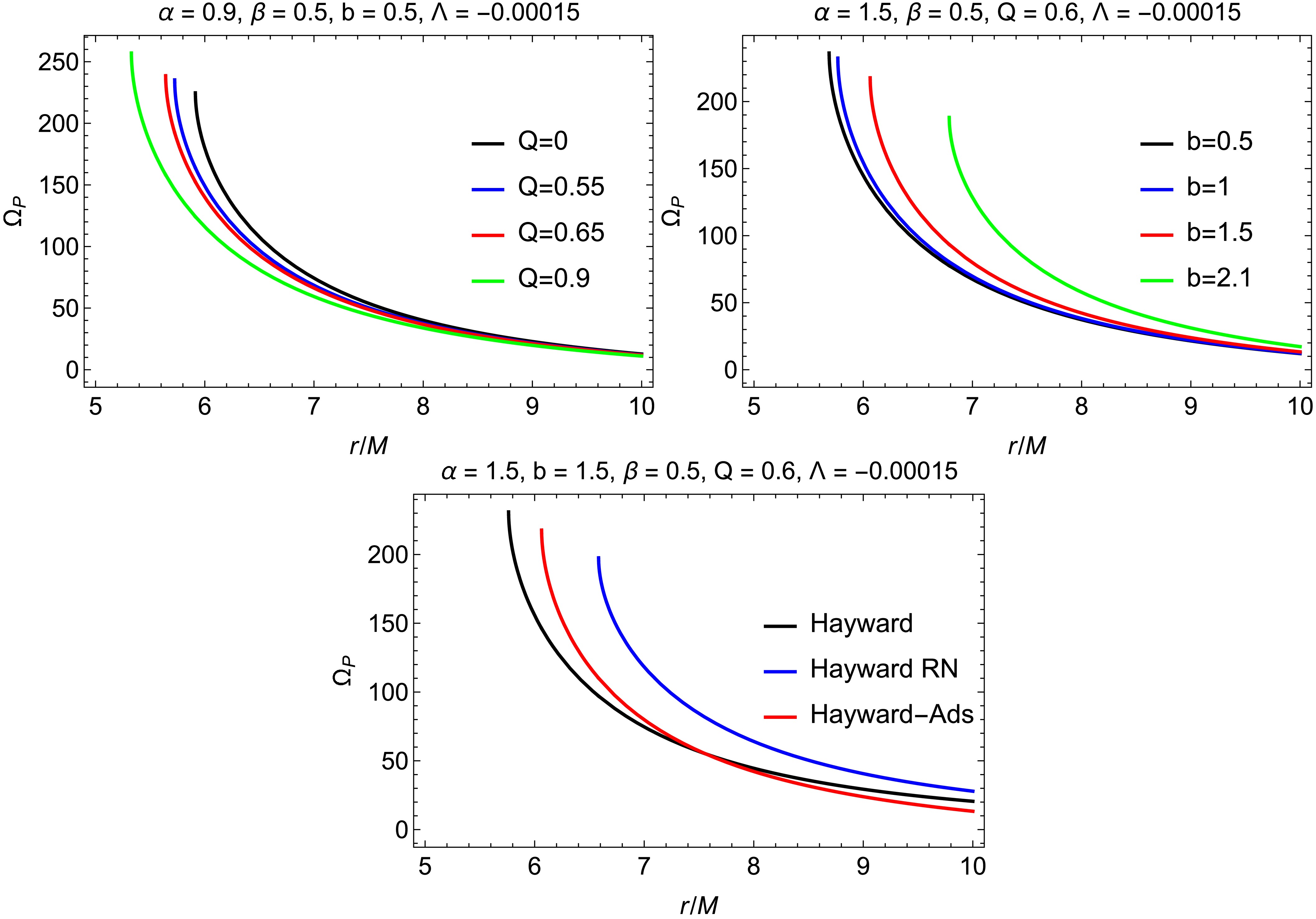
Figure 7. (color online) Periastron frequency of particles in the background of a Hayward-AdS BH within a fluid of strings.
The analysis presented above describes the dynamics of neutral test particles in the spacetime of a Hayward–AdS BH surrounded by a string fluid. In particular, the effective potential, circular orbits, ISCO structure, and epicyclic and precession frequencies collectively determine the orbital behavior of matter in this modified gravitational background. These quantities are closely related to observable phenomena in strong-gravity astrophysics, including accretion-disk dynamics and quasi-periodic oscillations.
However, the dynamical properties of a BH spacetime are determined not only by the motion of matter around it, but also by the way the spacetime itself responds to external perturbations. Small perturbations of the geometry generate damped oscillations known as quasinormal modes (QNMs), which characterize the relaxation of the spacetime after a disturbance and dominate the ringdown phase of gravitational-wave signals. Therefore, to obtain a more complete picture of the physical properties of the Hayward–AdS BH immersed in a string fluid, it is important to investigate its perturbative response. In the following section, we study electromagnetic perturbations of the spacetime and analyze the corresponding quasinormal-mode spectrum.
-
Here, we study the periastron frequency of a neutral test particle in the considered geometry under small perturbations constrained to the equatorial plane. It can be obtained as
$ \Omega_{P} = \Omega_{\phi} - \Omega_{r}. $
(29) Figure 7 shows how the periastron precession frequency of test particles changes when the Hayward–AdS BH is embedded in a fluid of strings. The periastron precession frequency exhibits a clear decreasing trend as the Hayward parameter
$ (Q) $ increases. This suggests that, as the regularization effects of the BH become stronger, the geometry produces weaker relativistic corrections to the particle motion. Increasing the radial distance shows a similar trend, which is physically reasonable because the relativistic effects that cause particle precession are strongest when the particles are closer to the BH and become more negligible at larger distances. Increasing the BH parameter$ (b) $ increases the periastron frequency because of the corresponding change in the spacetime geometry and the causally related changes in particle motion. An empirical observation is that particles moving in a fluid of strings in the presence of a Hayward–AdS BH exhibit less periastron precession than those in Hayward and Hayward–Reissner–Nordström BHs. This indicates that the AdS geometry and the surrounding cloud of strings reduce the gravitational field and the relativistic effects responsible for the precession.
Figure 7. (color online) Periastron frequency of particles in the background of a Hayward-AdS BH within a fluid of strings.
The analysis presented above describes the dynamics of neutral test particles in the spacetime of a Hayward–AdS BH surrounded by a string fluid. In particular, the effective potential, circular orbits, ISCO structure, and epicyclic and precession frequencies collectively determine the orbital behavior of matter in this modified gravitational background. These quantities are closely related to observable phenomena in strong-gravity astrophysics, including accretion-disk dynamics and quasi-periodic oscillations.
However, the dynamical properties of a BH spacetime are determined not only by the motion of matter around it, but also by the way the spacetime itself responds to external perturbations. Small perturbations of the geometry generate damped oscillations known as quasinormal modes (QNMs), which characterize the relaxation of the spacetime after a disturbance and dominate the ringdown phase of gravitational-wave signals. Therefore, to obtain a more complete picture of the physical properties of the Hayward–AdS BH immersed in a string fluid, it is important to investigate its perturbative response. In the following section, we study electromagnetic perturbations of the spacetime and analyze the corresponding quasinormal-mode spectrum.
-
The analysis presented in the previous sections focused on the geodesic dynamics of neutral test particles in the spacetime of a Hayward–AdS BH surrounded by a fluid of strings. In particular, the effective potential, circular orbits, ISCO structure, epicyclic oscillations, and periastron precession collectively characterize how matter moves in this modified gravitational background. These quantities are closely related to astrophysical observables, including accretion-disk dynamics and quasi-periodic oscillations, and therefore provide important insight into the strong-gravity properties of the spacetime.
While geodesic motion probes the behavior of matter in the background geometry, an equally important aspect of BH physics is the response of the spacetime itself to external perturbations. Small perturbations of the BH geometry generate damped oscillations known as quasinormal modes (QNMs), which dominate the ringdown phase of gravitational-wave signals following dynamical events such as BH mergers or perturbative excitations. The QNM spectrum therefore provides a complementary probe of the spacetime structure and stability. In the context of the present model, it is particularly interesting to investigate how the presence of the surrounding string fluid and the Hayward regularization parameter modify the oscillatory and dissipative properties of these perturbations.
Motivated by this connection, we now study electromagnetic perturbations of the Hayward–AdS BH immersed in a fluid of strings. This analysis allows us to explore the ringdown dynamics of the spacetime and to determine how the parameters governing the string fluid and the regular BH core influence the quasinormal-mode spectrum.
The Hayward–AdS BH, characterized by its regular core and anti-de Sitter asymptotics, is modified by the presence of a fluid of strings, which introduces additional parameters that affect the spacetime geometry. The fluid of strings contributes to the effective stress-energy tensor, thereby altering the metric function
$ h(r) $ and, consequently, the dynamics of perturbations. Our objective is to compute the quasinormal modes (QNMs) associated with electromagnetic perturbations using the Padé-averaged sixth-order Wentzel-Kramers-Brillouin (WKB) approximation and to assess the impact of the string fluid on the QNM spectrum. The electromagnetic perturbations are described by the radial wave equation:$ \partial^2_{r_*} \psi_{em}(r_*) + \omega^2 \psi_{em}(r_*) = V_{em}(r) \psi_{em}(r_*), $
(30) where
$ \psi_{em}(r_*) $ is the radial wave function,$ r_* $ is the tortoise coordinate defined by${\rm d}r_* = h(r)^{-1} {\rm d}r$ , and the effective potential is$ V_{em}(r) = h(r) \frac{l(l+1)}{r^2}. $
(31) This potential reflects the interplay among the regular core of the BH, the AdS background, and the string fluid, with the parameter α introducing a linear term that modifies the behavior of the potential, particularly at large radii.
To obtain the QNMs in our work, we use the Padé-averaged sixth-order WKB approximation, which provides reliable results with smaller errors. The WKB method, which offers a first-order approximation, was first introduced by Schutz and Will [79, 80]. However, in some cases this method yields relatively large errors; to address this issue, higher-order WKB approximations have been developed [81−83]. In the higher-order WKB approximation, the QNMs are given by the relation [82]
$ {\rm i}\frac{\left(\omega^{2}-V_{\text{max}}\right)}{\sqrt{-2V_{\text{max}}^{\prime\prime}}} - \sum\limits_{j=2}^{p}\Lambda_{j} = n + \dfrac{1}{2}, $
(32) where
$ V_{\text{max}} $ denotes the maximum value of the potential$ V_{em}(r) $ , and$ V_{\text{max}}^{\prime\prime} = \dfrac{{\rm d}^{2}V_{em}(r_{\ast})}{{\rm d} r_{\ast}^{2}}\bigg|_{r_{\ast}=r_{\text{max}}} $ .$ \Lambda_{j} $ denotes the higher-order WKB correction terms [82]. The term p in the summation denotes the order of the WKB approximation method; for the sixth-order WKB approximation,$ p=6 $ . For further details, one may refer to Refs. [81−83].The WKB method is particularly suitable for this analysis because it can handle the complex potential
$ V_{em}(r) $ and provide accurate estimates of the QNMs. The QNMs, denoted by$ \omega = \omega_r + i \omega_i $ , are characterized by their real part ($ \omega_r $ ), which represents the oscillation frequency, and their imaginary part ($ \omega_i $ ), which indicates the damping rate. The presence of the string fluid is expected to influence both components, potentially affecting the stability and oscillatory behavior of the perturbations.The numerical results for the QNMs are presented in Tables 2 and 3. These tables list the computed QNM frequencies for
$ \Lambda = -0.01 $ and$ \Lambda = 0.0 $ , together with various values of the multipole number l, the string-fluid parameter α, and the regularization parameter b. The tables also provide error estimates, including$ \vartriangle_{rms} $ and the error term$ \Delta_6 $ , defined asl WKB 6 $ \vartriangle_{rms} $ WKB 5 WKB 7 $ \Delta_6 $ 1 0.26645–0.0917256i 0.000123226 0.266335–0.0919119i 0.266401–0.0918343i 0.0000508874 2 0.487448–0.0944542i 0.0000253304 0.487441– 0.0944921i 0.487443–0.0944808i 5.712838717268585 $ \times 10^{-6} $ 3 0.698828–0.0952234i 5.845791870303999 $ \times 10^{-6} $ 0.698829–0.0952323i 0.698833–0.0952328i 1.7433653145548668 $ \times 10^{-6} $ 4 0.907145–0.0955445i 9.387634251921837 $ \times 10^{-8} $ 0.907144–0.0955442i 0.907145–0.0955443i 4.903375376210412 $ \times 10^{-7} $ 5 1.11407–0.0957036i 8.90389689392257 $ \times 10^{-8} $ 1.11408–0.095704i 1.11408–0.095704i 1.814090495215341 $ \times 10^{-7} $ 6 1.32027–0.0957961i 4.1348110278202216 $ \times 10^{-7} $ 1.32026–0.0957966i 1.32026–0.0957966i 8.370060920368116 $ \times 10^{-8} $ 7 1.52601–0.0958545i 4.4948485697971016 $ \times 10^{-8} $ 1.52601–0.0958547i 1.52601–0.0958547i 3.7776302713821793 $ \times 10^{-8} $ 8 1.73147–0.0958936i 1.5346681627146424 $ \times 10^{-7} $ 1.73147–0.0958937i 1.73147–0.0958938i 2.0464625335474405 $ \times 10^{-8} $ Table 2. Quasinormal modes of the BH with
$ n=0 $ ,$ \alpha=0.1 $ ,$ M=1 $ ,$ \beta=0.5 $ ,$ b=1 $ ,$ Q=0.5 $ , and$ \Lambda=-0.01 $ for electromagnetic perturbations. WKB 6, WKB 5, and WKB 7 in the column headings denote the quasinormal modes calculated using the sixth-, fifth-, and seventh-order WKB approximations, respectively.l WKB 6 $ \vartriangle_{rms} $ WKB 5 WKB 7 $ \Delta_6 $ 1 0.256335–0.0881115i 0.000218081 0.256029–0.0883249i 0.256091–0.0882578i 0.0000457315 2 0.467957–0.0906797i 0.0000220499 0.467941–0.090721i 0.467959–0.0907255i 9.167860822347937 $ \times 10^{-6} $ 3 0.670648–0.0913868i 5.293818420708917 $ \times 10^{-6} $ 0.670647–0.0913977i 0.67065–0.0913983i 1.6666035133093604 $ \times 10^{-6} $ 4 0.870438–0.0916779i 2.0842106066857143 $ \times 10^{-6} $ 0.870438–0.0916821i 0.870439–0.0916823i 4.7121688097006646 $ \times 10^{-7} $ 5 1.06892–0.0918258i 9.210535153965445 $ \times 10^{-7} $ 1.06892–0.0918275i 1.06892–0.0918276i 1.6130145698804756 $ \times 10^{-7} $ 6 1.2667–0.0919117i 1.969129482126316 $ \times 10^{-7} $ 1.2667–0.0919119i 1.2667–0.0919119i 7.404529708343354 $ \times 10^{-8} $ 7 1.46406–0.0919645i 2.0251870632419853 $ \times 10^{-7} $ 1.46406–0.0919649i 1.46406–0.0919649i 3.4198115199769346 $ \times 10^{-8} $ 8 1.66115–0.0920005i 2.002996014329446 $ \times 10^{-9} $ 1.66115–0.0920005i 1.66115–0.0920005i 1.9413475889090233 $ \times 10^{-8} $ Table 3. Quasinormal modes of the BH with
$ n=0 $ ,$ \alpha=0.1 $ ,$ M=1 $ ,$ \beta=0.5 $ ,$ b=1 $ ,$ Q=0.5 $ , and$ \Lambda=0 $ under electromagnetic perturbations.$ \Delta_6 = \frac{\left| \omega_7 - \omega_5 \right|}{2}, $
(33) where
$ \omega_7 $ and$ \omega_5 $ denote the QNM frequencies obtained from the 7th- and 5th-order Padé-averaged WKB approximations, respectively. The term$ \vartriangle_{rms} $ represents the root-mean-square error associated with the Padé averaging. These error metrics allow us to quantify the precision of our results and assess the reliability of the WKB method in this context. It may be noted that, as the multipole moment l increases, the errors associated with the QNMs decrease significantly. This is a characteristic of the WKB method, in which the error decreases with increasing$ (l-n) $ .Figures 8 and 9 illustrate the influence of the model parameters on the quasinormal mode (QNM) spectra. The first panel of Fig. 8 shows the dependence of the real part of the QNM frequency on the string fluid parameter α. The oscillation frequency corresponding to each ringdown gravitational-wave QNM, represented by the real part of the QNM frequency, exhibits an approximately linear dependence on α. More specifically, as α increases, the oscillation frequency decreases monotonically. This indicates that the effective string fluid parameter α reduces the effective restoring force associated with gravitational perturbations around the BH. The second panel of Fig. 8 shows the behavior of the imaginary part of the QNMs as a function of α. The imaginary part of the QNMs is associated with the damping (or decay) of the ringdown signal; thus, this result shows that, as α increases, the gravitational perturbations of the ringdown signal decay more rapidly. This suggests that the spacetime surrounded by string fluid effectively suppresses the perturbation and allows the spacetime to relax through energy dissipation more rapidly than it would in the absence of the string fluid. In summary, these results confirm that the string fluid parameter α contributes significantly to the structure of the QNM spectrum, specifically to the oscillatory and damping features of the ringdown gravitational waves. For small values of α, the QNMs closely resemble those of the standard Hayward-AdS BH, with the real part
$ \omega_r $ increasing with l and the imaginary part$ \omega_i $ indicating stable modes (negative values). As α increases, the linear term$ -\alpha r $ in$ h(r) $ reduces the potential barrier, leading to a decrease in$ \omega_r $ and a more negative$ \omega_i $ , suggesting higher damping rates. This behavior is consistent with the physical expectation that the string fluid introduces additional energy density, thereby altering the spacetime geometry and perturbation dynamics.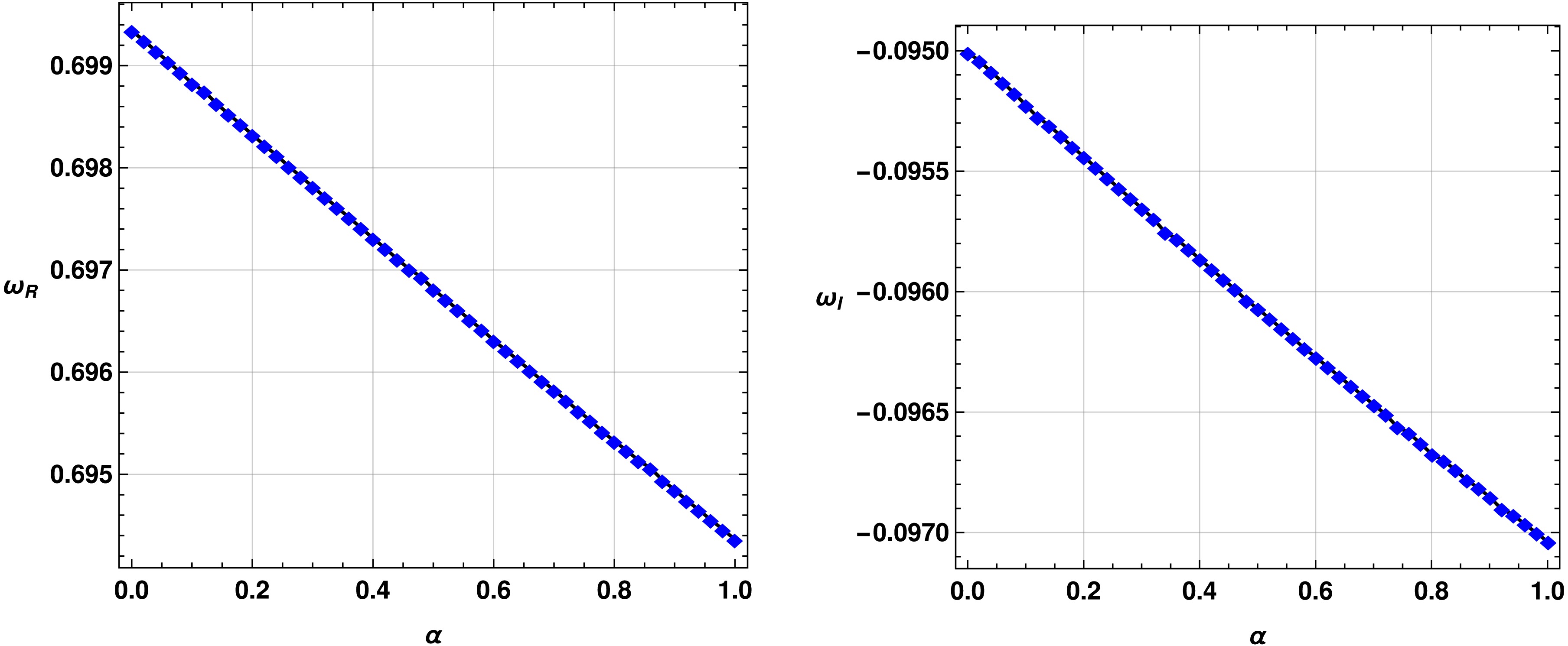
Figure 8. (color online) Variation of quasinormal modes with respect to the model parameter α for electromagnetic perturbations.
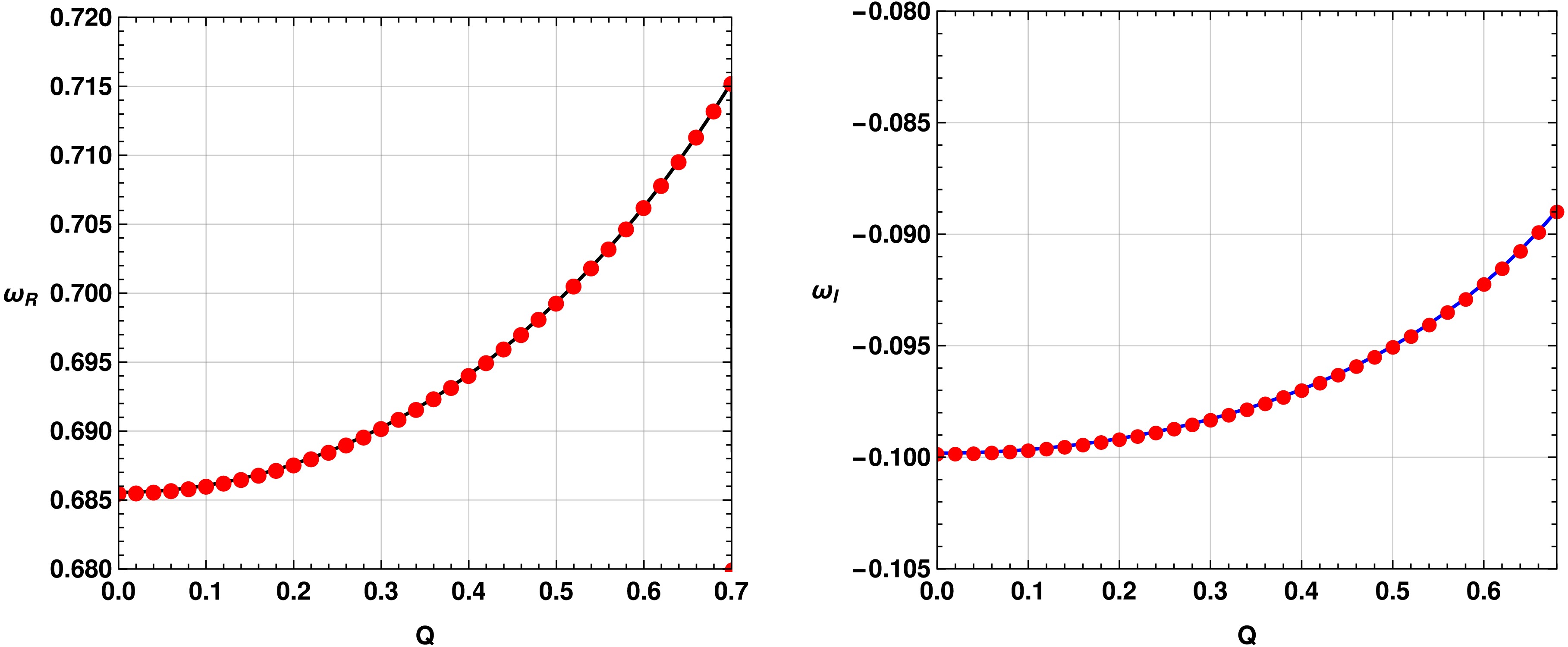
Figure 9. (color online) Variation of quasinormal modes with respect to the model parameter Q for electromagnetic perturbations.
In the first panel of Fig. 9, we show the impact of the Hayward parameter Q on the oscillation frequency of GWs. One can see that the effect of Q on the QNM spectrum is nonlinear. Fig. 9 shows the behavior of the quasinormal-mode frequencies. It indicates that the real part of the frequency
$\omega_R$ , for a given positive Hayward parameter Q, remains positive and increases nonlinearly. Thus, stronger regularization effects impart a more pronounced oscillatory pattern to the signal. This nonlinearity suggests a modification of the perturbation dynamics that is sensitive to changes in the near-horizon structure. In the second panel of Fig. 9, we see that as Q increases, the imaginary part of the frequency decreases nonlinearly; hence, the decay of the gravitational waves decreases. Larger values of Q lead to longer quasinormal ringing. In the present spacetime structure, the perturbations persist longer when the changes are more subtle. -
The analysis presented in the previous sections focused on the geodesic dynamics of neutral test particles in the spacetime of a Hayward–AdS BH surrounded by a fluid of strings. In particular, the effective potential, circular orbits, ISCO structure, epicyclic oscillations, and periastron precession collectively characterize how matter moves in this modified gravitational background. These quantities are closely related to astrophysical observables, including accretion-disk dynamics and quasi-periodic oscillations, and therefore provide important insight into the strong-gravity properties of the spacetime.
While geodesic motion probes the behavior of matter in the background geometry, an equally important aspect of BH physics is the response of the spacetime itself to external perturbations. Small perturbations of the BH geometry generate damped oscillations known as quasinormal modes (QNMs), which dominate the ringdown phase of gravitational-wave signals following dynamical events such as BH mergers or perturbative excitations. The QNM spectrum therefore provides a complementary probe of the spacetime structure and stability. In the context of the present model, it is particularly interesting to investigate how the presence of the surrounding string fluid and the Hayward regularization parameter modify the oscillatory and dissipative properties of these perturbations.
Motivated by this connection, we now study electromagnetic perturbations of the Hayward–AdS BH immersed in a fluid of strings. This analysis allows us to explore the ringdown dynamics of the spacetime and to determine how the parameters governing the string fluid and the regular BH core influence the quasinormal-mode spectrum.
The Hayward–AdS BH, characterized by its regular core and anti-de Sitter asymptotics, is modified by the presence of a fluid of strings, which introduces additional parameters that affect the spacetime geometry. The fluid of strings contributes to the effective stress-energy tensor, thereby altering the metric function
$ h(r) $ and, consequently, the dynamics of perturbations. Our objective is to compute the quasinormal modes (QNMs) associated with electromagnetic perturbations using the Padé-averaged sixth-order Wentzel-Kramers-Brillouin (WKB) approximation and to assess the impact of the string fluid on the QNM spectrum. The electromagnetic perturbations are described by the radial wave equation:$ \partial^2_{r_*} \psi_{em}(r_*) + \omega^2 \psi_{em}(r_*) = V_{em}(r) \psi_{em}(r_*), $
(30) where
$ \psi_{em}(r_*) $ is the radial wave function,$ r_* $ is the tortoise coordinate defined by${\rm d}r_* = h(r)^{-1} {\rm d}r$ , and the effective potential is$ V_{em}(r) = h(r) \frac{l(l+1)}{r^2}. $
(31) This potential reflects the interplay among the regular core of the BH, the AdS background, and the string fluid, with the parameter α introducing a linear term that modifies the behavior of the potential, particularly at large radii.
To obtain the QNMs in our work, we use the Padé-averaged sixth-order WKB approximation, which provides reliable results with smaller errors. The WKB method, which offers a first-order approximation, was first introduced by Schutz and Will [79, 80]. However, in some cases this method yields relatively large errors; to address this issue, higher-order WKB approximations have been developed [81−83]. In the higher-order WKB approximation, the QNMs are given by the relation [82]
$ {\rm i}\frac{\left(\omega^{2}-V_{\text{max}}\right)}{\sqrt{-2V_{\text{max}}^{\prime\prime}}} - \sum\limits_{j=2}^{p}\Lambda_{j} = n + \dfrac{1}{2}, $
(32) where
$ V_{\text{max}} $ denotes the maximum value of the potential$ V_{em}(r) $ , and$ V_{\text{max}}^{\prime\prime} = \dfrac{{\rm d}^{2}V_{em}(r_{\ast})}{{\rm d} r_{\ast}^{2}}\bigg|_{r_{\ast}=r_{\text{max}}} $ .$ \Lambda_{j} $ denotes the higher-order WKB correction terms [82]. The term p in the summation denotes the order of the WKB approximation method; for the sixth-order WKB approximation,$ p=6 $ . For further details, one may refer to Refs. [81−83].The WKB method is particularly suitable for this analysis because it can handle the complex potential
$ V_{em}(r) $ and provide accurate estimates of the QNMs. The QNMs, denoted by$ \omega = \omega_r + i \omega_i $ , are characterized by their real part ($ \omega_r $ ), which represents the oscillation frequency, and their imaginary part ($ \omega_i $ ), which indicates the damping rate. The presence of the string fluid is expected to influence both components, potentially affecting the stability and oscillatory behavior of the perturbations.The numerical results for the QNMs are presented in Tables 2 and 3. These tables list the computed QNM frequencies for
$ \Lambda = -0.01 $ and$ \Lambda = 0.0 $ , together with various values of the multipole number l, the string-fluid parameter α, and the regularization parameter b. The tables also provide error estimates, including$ \vartriangle_{rms} $ and the error term$ \Delta_6 $ , defined asl WKB 6 $ \vartriangle_{rms} $ WKB 5 WKB 7 $ \Delta_6 $ 1 0.26645–0.0917256i 0.000123226 0.266335–0.0919119i 0.266401–0.0918343i 0.0000508874 2 0.487448–0.0944542i 0.0000253304 0.487441– 0.0944921i 0.487443–0.0944808i 5.712838717268585 $ \times 10^{-6} $ 3 0.698828–0.0952234i 5.845791870303999 $ \times 10^{-6} $ 0.698829–0.0952323i 0.698833–0.0952328i 1.7433653145548668 $ \times 10^{-6} $ 4 0.907145–0.0955445i 9.387634251921837 $ \times 10^{-8} $ 0.907144–0.0955442i 0.907145–0.0955443i 4.903375376210412 $ \times 10^{-7} $ 5 1.11407–0.0957036i 8.90389689392257 $ \times 10^{-8} $ 1.11408–0.095704i 1.11408–0.095704i 1.814090495215341 $ \times 10^{-7} $ 6 1.32027–0.0957961i 4.1348110278202216 $ \times 10^{-7} $ 1.32026–0.0957966i 1.32026–0.0957966i 8.370060920368116 $ \times 10^{-8} $ 7 1.52601–0.0958545i 4.4948485697971016 $ \times 10^{-8} $ 1.52601–0.0958547i 1.52601–0.0958547i 3.7776302713821793 $ \times 10^{-8} $ 8 1.73147–0.0958936i 1.5346681627146424 $ \times 10^{-7} $ 1.73147–0.0958937i 1.73147–0.0958938i 2.0464625335474405 $ \times 10^{-8} $ Table 2. Quasinormal modes of the BH with
$ n=0 $ ,$ \alpha=0.1 $ ,$ M=1 $ ,$ \beta=0.5 $ ,$ b=1 $ ,$ Q=0.5 $ , and$ \Lambda=-0.01 $ for electromagnetic perturbations. WKB 6, WKB 5, and WKB 7 in the column headings denote the quasinormal modes calculated using the sixth-, fifth-, and seventh-order WKB approximations, respectively.l WKB 6 $ \vartriangle_{rms} $ WKB 5 WKB 7 $ \Delta_6 $ 1 0.256335–0.0881115i 0.000218081 0.256029–0.0883249i 0.256091–0.0882578i 0.0000457315 2 0.467957–0.0906797i 0.0000220499 0.467941–0.090721i 0.467959–0.0907255i 9.167860822347937 $ \times 10^{-6} $ 3 0.670648–0.0913868i 5.293818420708917 $ \times 10^{-6} $ 0.670647–0.0913977i 0.67065–0.0913983i 1.6666035133093604 $ \times 10^{-6} $ 4 0.870438–0.0916779i 2.0842106066857143 $ \times 10^{-6} $ 0.870438–0.0916821i 0.870439–0.0916823i 4.7121688097006646 $ \times 10^{-7} $ 5 1.06892–0.0918258i 9.210535153965445 $ \times 10^{-7} $ 1.06892–0.0918275i 1.06892–0.0918276i 1.6130145698804756 $ \times 10^{-7} $ 6 1.2667–0.0919117i 1.969129482126316 $ \times 10^{-7} $ 1.2667–0.0919119i 1.2667–0.0919119i 7.404529708343354 $ \times 10^{-8} $ 7 1.46406–0.0919645i 2.0251870632419853 $ \times 10^{-7} $ 1.46406–0.0919649i 1.46406–0.0919649i 3.4198115199769346 $ \times 10^{-8} $ 8 1.66115–0.0920005i 2.002996014329446 $ \times 10^{-9} $ 1.66115–0.0920005i 1.66115–0.0920005i 1.9413475889090233 $ \times 10^{-8} $ Table 3. Quasinormal modes of the BH with
$ n=0 $ ,$ \alpha=0.1 $ ,$ M=1 $ ,$ \beta=0.5 $ ,$ b=1 $ ,$ Q=0.5 $ , and$ \Lambda=0 $ under electromagnetic perturbations.$ \Delta_6 = \frac{\left| \omega_7 - \omega_5 \right|}{2}, $
(33) where
$ \omega_7 $ and$ \omega_5 $ denote the QNM frequencies obtained from the 7th- and 5th-order Padé-averaged WKB approximations, respectively. The term$ \vartriangle_{rms} $ represents the root-mean-square error associated with the Padé averaging. These error metrics allow us to quantify the precision of our results and assess the reliability of the WKB method in this context. It may be noted that, as the multipole moment l increases, the errors associated with the QNMs decrease significantly. This is a characteristic of the WKB method, in which the error decreases with increasing$ (l-n) $ .Figures 8 and 9 illustrate the influence of the model parameters on the quasinormal mode (QNM) spectra. The first panel of Fig. 8 shows the dependence of the real part of the QNM frequency on the string fluid parameter α. The oscillation frequency corresponding to each ringdown gravitational-wave QNM, represented by the real part of the QNM frequency, exhibits an approximately linear dependence on α. More specifically, as α increases, the oscillation frequency decreases monotonically. This indicates that the effective string fluid parameter α reduces the effective restoring force associated with gravitational perturbations around the BH. The second panel of Fig. 8 shows the behavior of the imaginary part of the QNMs as a function of α. The imaginary part of the QNMs is associated with the damping (or decay) of the ringdown signal; thus, this result shows that, as α increases, the gravitational perturbations of the ringdown signal decay more rapidly. This suggests that the spacetime surrounded by string fluid effectively suppresses the perturbation and allows the spacetime to relax through energy dissipation more rapidly than it would in the absence of the string fluid. In summary, these results confirm that the string fluid parameter α contributes significantly to the structure of the QNM spectrum, specifically to the oscillatory and damping features of the ringdown gravitational waves. For small values of α, the QNMs closely resemble those of the standard Hayward-AdS BH, with the real part
$ \omega_r $ increasing with l and the imaginary part$ \omega_i $ indicating stable modes (negative values). As α increases, the linear term$ -\alpha r $ in$ h(r) $ reduces the potential barrier, leading to a decrease in$ \omega_r $ and a more negative$ \omega_i $ , suggesting higher damping rates. This behavior is consistent with the physical expectation that the string fluid introduces additional energy density, thereby altering the spacetime geometry and perturbation dynamics.
Figure 8. (color online) Variation of quasinormal modes with respect to the model parameter α for electromagnetic perturbations.
Figure 9. (color online) Variation of quasinormal modes with respect to the model parameter Q for electromagnetic perturbations.
In the first panel of Fig. 9, we show the impact of the Hayward parameter Q on the oscillation frequency of GWs. One can see that the effect of Q on the QNM spectrum is nonlinear. Fig. 9 shows the behavior of the quasinormal-mode frequencies. It indicates that the real part of the frequency
$\omega_R$ , for a given positive Hayward parameter Q, remains positive and increases nonlinearly. Thus, stronger regularization effects impart a more pronounced oscillatory pattern to the signal. This nonlinearity suggests a modification of the perturbation dynamics that is sensitive to changes in the near-horizon structure. In the second panel of Fig. 9, we see that as Q increases, the imaginary part of the frequency decreases nonlinearly; hence, the decay of the gravitational waves decreases. Larger values of Q lead to longer quasinormal ringing. In the present spacetime structure, the perturbations persist longer when the changes are more subtle. -
In this section, we present a detailed analysis of the time-domain evolution of electromagnetic perturbations in the background of the Hayward-AdS BH immersed in a fluid of strings. Although frequency-domain calculations of QNMs provide insight into the oscillatory and damping properties, a complete understanding of the dynamical response requires a direct investigation of the temporal evolution of the perturbation. To this end, we implement a time-domain integration scheme based on the characteristic method developed by Gundlach et al. [84], following an approach similar to that used in [85].
The evolution of the perturbation field
$ \psi(r_*,t) $ is governed by the wave equation$ \frac{\partial^2 \psi}{\partial t^2} - \frac{\partial^2 \psi}{\partial r_*^2} + V(r) \psi = 0, $
(34) where
$ V(r) $ is the effective potential and$ r_* $ is the tortoise coordinate.We discretize the wave equation using a second-order finite difference scheme:
$ \frac{\psi_{i+1,j} - 2\psi_{i,j} + \psi_{i-1,j}}{\Delta r_*^2} - \frac{\psi_{i,j+1} - 2\psi_{i,j} + \psi_{i,j-1}}{\Delta t^2} - V_i \psi_{i,j} = 0, $
(35) where
$ \Delta t $ and$ \Delta r_* $ denote the time and spatial grid spacings, respectively, and the Courant-Friedrichs-Lewy (CFL) stability condition$ \Delta t / \Delta r_* \lt 1 $ is imposed (here, we consider$ \Delta t / \Delta r_* =0.7 $ ).The initial conditions are specified by a Gaussian wave packet centered near the event horizon:
$ \psi(r_*, 0) = \exp\left[ -\frac{(r_* - k_1)^2}{2 \sigma^2} \right], \quad \left. \frac{\partial \psi}{\partial t} \right|_{t=0} = 0, $
(36) where
$ k_1 $ and σ determine the location and width of the initial perturbation. Here, we choose$ \sigma=5 $ and$ k_1 = 0. $ The time evolution is then computed iteratively according to$ \begin{split} \psi_{i,j+1} =& -\psi_{i,j-1} + \left( \frac{\Delta t}{\Delta r_*} \right)^2 (\psi_{i+1,j} + \psi_{i-1,j})\\ & + \left(2 - 2\left( \frac{\Delta t}{\Delta r_*} \right)^2 - V_i \Delta t^2\right)\psi_{i,j}. \end{split} $
(37) -
In this section, we present a detailed analysis of the time-domain evolution of electromagnetic perturbations in the background of the Hayward-AdS BH immersed in a fluid of strings. Although frequency-domain calculations of QNMs provide insight into the oscillatory and damping properties, a complete understanding of the dynamical response requires a direct investigation of the temporal evolution of the perturbation. To this end, we implement a time-domain integration scheme based on the characteristic method developed by Gundlach et al. [84], following an approach similar to that used in [85].
The evolution of the perturbation field
$ \psi(r_*,t) $ is governed by the wave equation$ \frac{\partial^2 \psi}{\partial t^2} - \frac{\partial^2 \psi}{\partial r_*^2} + V(r) \psi = 0, $
(34) where
$ V(r) $ is the effective potential and$ r_* $ is the tortoise coordinate.We discretize the wave equation using a second-order finite difference scheme:
$ \frac{\psi_{i+1,j} - 2\psi_{i,j} + \psi_{i-1,j}}{\Delta r_*^2} - \frac{\psi_{i,j+1} - 2\psi_{i,j} + \psi_{i,j-1}}{\Delta t^2} - V_i \psi_{i,j} = 0, $
(35) where
$ \Delta t $ and$ \Delta r_* $ denote the time and spatial grid spacings, respectively, and the Courant-Friedrichs-Lewy (CFL) stability condition$ \Delta t / \Delta r_* \lt 1 $ is imposed (here, we consider$ \Delta t / \Delta r_* =0.7 $ ).The initial conditions are specified by a Gaussian wave packet centered near the event horizon:
$ \psi(r_*, 0) = \exp\left[ -\frac{(r_* - k_1)^2}{2 \sigma^2} \right], \quad \left. \frac{\partial \psi}{\partial t} \right|_{t=0} = 0, $
(36) where
$ k_1 $ and σ determine the location and width of the initial perturbation. Here, we choose$ \sigma=5 $ and$ k_1 = 0. $ The time evolution is then computed iteratively according to$ \begin{split} \psi_{i,j+1} =& -\psi_{i,j-1} + \left( \frac{\Delta t}{\Delta r_*} \right)^2 (\psi_{i+1,j} + \psi_{i-1,j})\\ & + \left(2 - 2\left( \frac{\Delta t}{\Delta r_*} \right)^2 - V_i \Delta t^2\right)\psi_{i,j}. \end{split} $
(37) -
The time evolution of electromagnetic perturbations exhibits two distinct stages. Initially, the perturbation undergoes a ringdown phase dominated by the fundamental quasinormal mode and characterized by exponentially damped oscillations. Subsequently, the amplitude decays exponentially without transitioning to a power-law tail, consistent with the reflective nature of asymptotically AdS boundary conditions.
The obtained time-domain profiles are presented in Fig. 10. The influence of various parameters on the evolution is analyzed systematically:
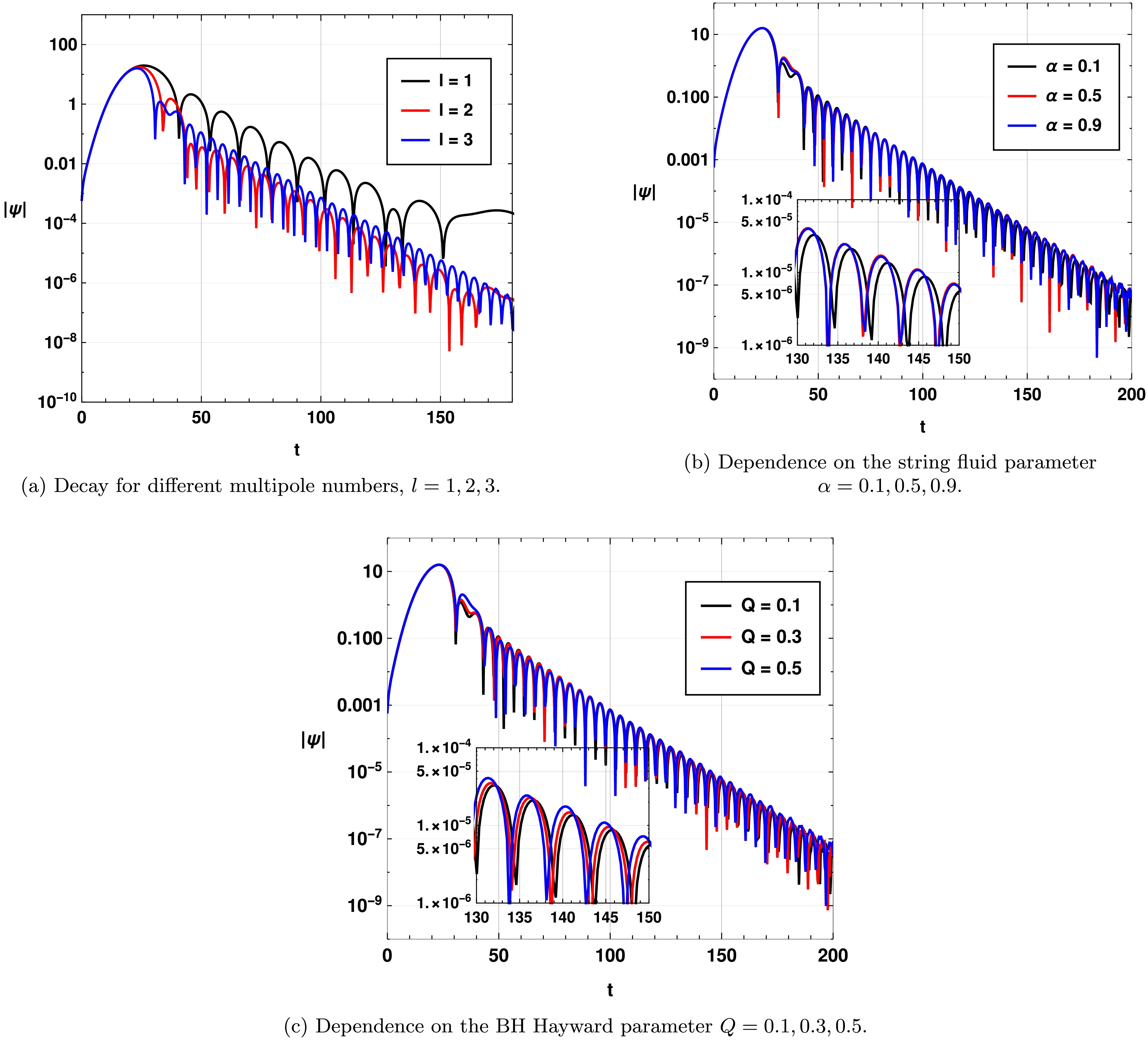
Figure 10. (color online) Time-domain profiles of electromagnetic perturbations around the Hayward-AdS BH immersed in a fluid of strings. In all cases, the profiles exhibit an initial ringdown phase followed by purely exponential decay, with no evidence of power-law tails or echo-like structures.
● As shown in Fig. 10(a), increasing the multipole number l results in higher oscillation frequencies and faster decay rates, consistent with the behavior expected of modes with higher angular momentum.
● In Fig. 10(b), the effect of varying the string fluid parameter α is illustrated. Larger values of α increase the damping of perturbations, resulting in a faster exponential decay at late times.
● Fig. 10(c) illustrates the impact of the BH Hayward parameter Q on the evolution. Higher values of Q tend to delay the transition to the final exponential decay phase and to slightly modulate the amplitude of the oscillations during the ringdown.
-
The time evolution of electromagnetic perturbations exhibits two distinct stages. Initially, the perturbation undergoes a ringdown phase dominated by the fundamental quasinormal mode and characterized by exponentially damped oscillations. Subsequently, the amplitude decays exponentially without transitioning to a power-law tail, consistent with the reflective nature of asymptotically AdS boundary conditions.
The obtained time-domain profiles are presented in Fig. 10. The influence of various parameters on the evolution is analyzed systematically:
Figure 10. (color online) Time-domain profiles of electromagnetic perturbations around the Hayward-AdS BH immersed in a fluid of strings. In all cases, the profiles exhibit an initial ringdown phase followed by purely exponential decay, with no evidence of power-law tails or echo-like structures.
● As shown in Fig. 10(a), increasing the multipole number l results in higher oscillation frequencies and faster decay rates, consistent with the behavior expected of modes with higher angular momentum.
● In Fig. 10(b), the effect of varying the string fluid parameter α is illustrated. Larger values of α increase the damping of perturbations, resulting in a faster exponential decay at late times.
● Fig. 10(c) illustrates the impact of the BH Hayward parameter Q on the evolution. Higher values of Q tend to delay the transition to the final exponential decay phase and to slightly modulate the amplitude of the oscillations during the ringdown.
-
The time-domain evolution confirms the stability of the Hayward-AdS BH immersed in a fluid of strings under electromagnetic perturbations. The perturbations decay exponentially after the ringdown phase, with no signatures of power-law tails or echo-like features. The decay rates and oscillatory behavior are significantly influenced by the multipole number l, the string fluid density α, and the BH Hayward parameter Q, providing a comprehensive picture of the system's dynamical response.
Understanding the time-domain profiles of vector perturbations reveals that the phenomenology is quite complex. There is a QNM-dominated ringdown, power-law tails modified by the AdS boundary, and echo-like structures driven by the Hayward regularization and the string fluid. This rich set of features is significant for the distinctive dynamics, stability, and possible astrophysical implications of the Hayward-AdS BH in a string fluid.
-
The time-domain evolution confirms the stability of the Hayward-AdS BH immersed in a fluid of strings under electromagnetic perturbations. The perturbations decay exponentially after the ringdown phase, with no signatures of power-law tails or echo-like features. The decay rates and oscillatory behavior are significantly influenced by the multipole number l, the string fluid density α, and the BH Hayward parameter Q, providing a comprehensive picture of the system's dynamical response.
Understanding the time-domain profiles of vector perturbations reveals that the phenomenology is quite complex. There is a QNM-dominated ringdown, power-law tails modified by the AdS boundary, and echo-like structures driven by the Hayward regularization and the string fluid. This rich set of features is significant for the distinctive dynamics, stability, and possible astrophysical implications of the Hayward-AdS BH in a string fluid.
-
In this work, we studied the Hayward-AdS BH spacetime modified by the presence of a surrounding fluid of strings. The Hayward parameter Q and the string fluid parameters α and b are of particular importance to our analysis. We are primarily interested in the geodesic motion of test particles, the properties of epicyclic oscillations, and the response of the spacetime to a massless vector (electromagnetic) perturbation through the quasinormal mode (QNM) spectrum. Finally, we aim to examine the phenomena that arise in the vicinity of a BH.
Our study of particle dynamics revealed a strong dependence on the geometric parameters of the BH. We found that the Hayward parameter Q, which regularizes the central singularity, has a significant effect on stable circular orbits. An increase in Q decreases the specific energy and angular momentum required for a particle to maintain a circular orbit at a given radius. Consequently, the innermost stable circular orbit (ISCO) shifts closer to the BH as Q increases. In contrast, the string parameter b has the opposite effect, increasing the particle energy, angular momentum, and ISCO radius. This indicates a competitive interplay between the regularizing effect of the Hayward parameter and the influence of the string fluid. Furthermore, our analysis of the frequency of periastron precession showed that it decreases with increasing Q but increases with increasing b, providing another potential observable for distinguishing the effects of these parameters.
The examination of epicyclic frequencies, which are astrophysically linked to quasi-periodic oscillations (QPOs) observed in accretion disks, further reinforced these findings. We derived the radial, vertical, and orbital frequencies as measured by both local and distant observers. The results showed that these fundamental frequencies are sensitive probes of the underlying spacetime. The distinct dependencies of the epicyclic frequencies on Q and the string parameters suggest that precise QPO measurements could, in principle, be used to constrain the properties of such a regular BH and its surrounding environment. Comparison with standard Hayward and Hayward Reissner Nordström BHs demonstrated that the fluid of strings introduces unique modifications to particle trajectories and their associated frequencies.
In the final part of our analysis, we investigated the QNMs arising from massless vector perturbations. Employing the 6th-order WKB approximation, we found that the Hayward parameter Q and the string fluid parameter α have opposing effects on the resulting ringdown gravitational-wave signal. Specifically, an increase in Q leads to a non-linear increase in the oscillation frequency (
$ \omega_R $ ) and a decrease in the damping rate ($ |\omega_I| $ ), implying that the regularization causes the BH to "ring" for a longer time.Together, these complementary analyses provide a rich phenomenological picture of the Hayward-AdS BH within a fluid of strings. The opposing influences of the Hayward parameter and the string fluid on various observables—from ISCO radii to QNM damping times—highlight a potential degeneracy problem. Disentangling these effects would likely require a multi-messenger approach, combining information from accretion-disk phenomena (QPOs), BH shadow imaging, and gravitational-wave spectroscopy. Our detailed theoretical investigation provides the necessary framework and predictive templates for such future observational tests, paving the way for a deeper understanding of regular BHs and the fundamental nature of spacetime in the strong-field regime.
A particularly profound physical implication arises from the effect of the Hayward parameter Q on the QNM damping rate. The parameter Q encapsulates the deviation from classical General Relativity by resolving the central singularity, a feature often attributed to the effects of underlying quantum gravity. Our finding that an increased Q leads to a smaller damping rate (
$ |\omega_I| $ ) suggests that these quantum-regularized BHs are less efficient radiators of gravitational waves than their singular counterparts. Physically, the singularity in a classical BH can be viewed as an infinitely effective sink for information and energy. By smoothing out this singularity, the regular BH spacetime becomes "less absorptive" or "less lossy". Consequently, perturbations are not dissipated as quickly, allowing the BH to oscillate, or "ring", for a longer duration. This raises the tantalizing possibility that the damping time of a ringdown signal could be a direct probe of quantum-gravity corrections near the BH core.In direct contrast, the string fluid parameter α introduces a distinct physical effect on the spacetime. The fluid of strings acts as an external matter field, and our results show that increasing its density (a larger α) enhances the damping of perturbations. This behavior can be interpreted as a dissipative effect, analogous to that of a mechanical oscillator submerged in a viscous medium. The surrounding string fluid provides an additional channel through which the perturbed BH can shed energy, causing it to settle back to equilibrium more rapidly. This highlights the crucial role that the BH's immediate environment can play in shaping its gravitational-wave signal. It suggests that the observed ringdown is a convolution of the intrinsic properties of the BH (governed by M and Q) and the dissipative effects of its surroundings (governed by α).
The opposing influences of Q and α on the QNM spectrum pose a significant challenge because of observational degeneracy. A gravitational-wave signal with a specific frequency and damping time might be attributable either to a BH with a high degree of quantum regularization (large Q) in a sparse string fluid (low α) or, alternatively, to a more classical BH (low Q) immersed in a dense string fluid (high α). This ambiguity makes it difficult to uniquely determine the nature of the object from its QNM spectrum alone. Breaking this degeneracy is therefore paramount for accurately interpreting future observations. It necessitates a multi-pronged observational strategy in which data from different physical processes are combined. For example, while QNMs probe the dynamical response, observations of the BH shadow via Very Long Baseline interferometry could independently constrain the geometric parameter Q, while X-ray observations of QPOs from an accretion disk could constrain the particle dynamics influenced by both Q and the string parameters.
Looking forward, several avenues for future research are clearly indicated by our findings. Our analysis was restricted to a non-rotating, spherically symmetric spacetime. A crucial next step is to generalize this model to a rotating Kerr-like Hayward-AdS BH. The introduction of rotation would induce frame dragging and allow for phenomena such as superradiance, which would profoundly affect particle orbits, QPOs, and the QNM spectrum, thereby making the model more astrophysically realistic. Furthermore, this work focused on electromagnetic perturbations. A complete stability analysis requires the investigation of scalar and, most importantly, tensor (gravitational) perturbations. The QNMs of tensor perturbations are what gravitational-wave detectors directly measure, and calculating their spectrum for this model is essential for creating accurate templates for data analysis. Such an investigation would reveal whether the opposing effects of Q and α persist for gravitational waves themselves.
Beyond dynamical perturbations, the thermodynamic properties of this spacetime offer another rich area for exploration. Investigating how the parameters Q and α modify the BH's entropy, Hawking temperature, and the information paradox would connect the classical phenomena studied here to the deep questions of quantum gravity and BH information. In summary, this study not only characterizes a specific regular BH model but also provides a clear roadmap for future theoretical and observational work aimed at probing the nexus of gravity, quantum effects, and exotic matter fields in the universe's most extreme environments.
-
In this work, we studied the Hayward-AdS BH spacetime modified by the presence of a surrounding fluid of strings. The Hayward parameter Q and the string fluid parameters α and b are of particular importance to our analysis. We are primarily interested in the geodesic motion of test particles, the properties of epicyclic oscillations, and the response of the spacetime to a massless vector (electromagnetic) perturbation through the quasinormal mode (QNM) spectrum. Finally, we aim to examine the phenomena that arise in the vicinity of a BH.
Our study of particle dynamics revealed a strong dependence on the geometric parameters of the BH. We found that the Hayward parameter Q, which regularizes the central singularity, has a significant effect on stable circular orbits. An increase in Q decreases the specific energy and angular momentum required for a particle to maintain a circular orbit at a given radius. Consequently, the innermost stable circular orbit (ISCO) shifts closer to the BH as Q increases. In contrast, the string parameter b has the opposite effect, increasing the particle energy, angular momentum, and ISCO radius. This indicates a competitive interplay between the regularizing effect of the Hayward parameter and the influence of the string fluid. Furthermore, our analysis of the frequency of periastron precession showed that it decreases with increasing Q but increases with increasing b, providing another potential observable for distinguishing the effects of these parameters.
The examination of epicyclic frequencies, which are astrophysically linked to quasi-periodic oscillations (QPOs) observed in accretion disks, further reinforced these findings. We derived the radial, vertical, and orbital frequencies as measured by both local and distant observers. The results showed that these fundamental frequencies are sensitive probes of the underlying spacetime. The distinct dependencies of the epicyclic frequencies on Q and the string parameters suggest that precise QPO measurements could, in principle, be used to constrain the properties of such a regular BH and its surrounding environment. Comparison with standard Hayward and Hayward Reissner Nordström BHs demonstrated that the fluid of strings introduces unique modifications to particle trajectories and their associated frequencies.
In the final part of our analysis, we investigated the QNMs arising from massless vector perturbations. Employing the 6th-order WKB approximation, we found that the Hayward parameter Q and the string fluid parameter α have opposing effects on the resulting ringdown gravitational-wave signal. Specifically, an increase in Q leads to a non-linear increase in the oscillation frequency (
$ \omega_R $ ) and a decrease in the damping rate ($ |\omega_I| $ ), implying that the regularization causes the BH to "ring" for a longer time.Together, these complementary analyses provide a rich phenomenological picture of the Hayward-AdS BH within a fluid of strings. The opposing influences of the Hayward parameter and the string fluid on various observables—from ISCO radii to QNM damping times—highlight a potential degeneracy problem. Disentangling these effects would likely require a multi-messenger approach, combining information from accretion-disk phenomena (QPOs), BH shadow imaging, and gravitational-wave spectroscopy. Our detailed theoretical investigation provides the necessary framework and predictive templates for such future observational tests, paving the way for a deeper understanding of regular BHs and the fundamental nature of spacetime in the strong-field regime.
A particularly profound physical implication arises from the effect of the Hayward parameter Q on the QNM damping rate. The parameter Q encapsulates the deviation from classical General Relativity by resolving the central singularity, a feature often attributed to the effects of underlying quantum gravity. Our finding that an increased Q leads to a smaller damping rate (
$ |\omega_I| $ ) suggests that these quantum-regularized BHs are less efficient radiators of gravitational waves than their singular counterparts. Physically, the singularity in a classical BH can be viewed as an infinitely effective sink for information and energy. By smoothing out this singularity, the regular BH spacetime becomes "less absorptive" or "less lossy". Consequently, perturbations are not dissipated as quickly, allowing the BH to oscillate, or "ring", for a longer duration. This raises the tantalizing possibility that the damping time of a ringdown signal could be a direct probe of quantum-gravity corrections near the BH core.In direct contrast, the string fluid parameter α introduces a distinct physical effect on the spacetime. The fluid of strings acts as an external matter field, and our results show that increasing its density (a larger α) enhances the damping of perturbations. This behavior can be interpreted as a dissipative effect, analogous to that of a mechanical oscillator submerged in a viscous medium. The surrounding string fluid provides an additional channel through which the perturbed BH can shed energy, causing it to settle back to equilibrium more rapidly. This highlights the crucial role that the BH's immediate environment can play in shaping its gravitational-wave signal. It suggests that the observed ringdown is a convolution of the intrinsic properties of the BH (governed by M and Q) and the dissipative effects of its surroundings (governed by α).
The opposing influences of Q and α on the QNM spectrum pose a significant challenge because of observational degeneracy. A gravitational-wave signal with a specific frequency and damping time might be attributable either to a BH with a high degree of quantum regularization (large Q) in a sparse string fluid (low α) or, alternatively, to a more classical BH (low Q) immersed in a dense string fluid (high α). This ambiguity makes it difficult to uniquely determine the nature of the object from its QNM spectrum alone. Breaking this degeneracy is therefore paramount for accurately interpreting future observations. It necessitates a multi-pronged observational strategy in which data from different physical processes are combined. For example, while QNMs probe the dynamical response, observations of the BH shadow via Very Long Baseline interferometry could independently constrain the geometric parameter Q, while X-ray observations of QPOs from an accretion disk could constrain the particle dynamics influenced by both Q and the string parameters.
Looking forward, several avenues for future research are clearly indicated by our findings. Our analysis was restricted to a non-rotating, spherically symmetric spacetime. A crucial next step is to generalize this model to a rotating Kerr-like Hayward-AdS BH. The introduction of rotation would induce frame dragging and allow for phenomena such as superradiance, which would profoundly affect particle orbits, QPOs, and the QNM spectrum, thereby making the model more astrophysically realistic. Furthermore, this work focused on electromagnetic perturbations. A complete stability analysis requires the investigation of scalar and, most importantly, tensor (gravitational) perturbations. The QNMs of tensor perturbations are what gravitational-wave detectors directly measure, and calculating their spectrum for this model is essential for creating accurate templates for data analysis. Such an investigation would reveal whether the opposing effects of Q and α persist for gravitational waves themselves.
Beyond dynamical perturbations, the thermodynamic properties of this spacetime offer another rich area for exploration. Investigating how the parameters Q and α modify the BH's entropy, Hawking temperature, and the information paradox would connect the classical phenomena studied here to the deep questions of quantum gravity and BH information. In summary, this study not only characterizes a specific regular BH model but also provides a clear roadmap for future theoretical and observational work aimed at probing the nexus of gravity, quantum effects, and exotic matter fields in the universe's most extreme environments.
Frequencies spectra and gravitational ringing around Hayward-AdS black holes immersed in a string fluid
- Received Date: 2026-02-02
- Available Online: 2026-11-15
Abstract: We investigate the dynamics of test particles in a Hayward–AdS black hole with string fluid, with particular emphasis on how the relevant parameters influence particle motion. The stability of circular orbits is studied using the effective potential method, which yields analytic expressions for the particle energy and angular momentum in terms of the black hole parameters. The effects of these parameters on the innermost stable circular orbit and the effective force are also examined. In addition, we calculate the pericenter precession frequency and investigate the small oscillatory motion of a particle around a stable orbit, examining how the corresponding frequency is modified by the black hole parameters. We further compare particle dynamics in the Hayward–AdS spacetime with string fluid to those in the Hayward–AdS, the Hayward Reissner Nordstrom, and the conventional Hayward black holes. Lastly, we examine the influence of the string fluid and the Hayward parameter on the quasinormal spectrum and the time-domain dynamics of electromagnetic perturbations, and find that these two terms have reciprocal effects on the quasinormal scale.



 DownLoad: