


 Abstract
 HTML
HTML Reference
 Related
 PDF
PDF


-
The equation of state (EOS) of cold dense matter is a central problem in nuclear physics, astrophysics, and gravitational-wave astronomy. It determines the structure and composition of neutron stars, including their maximum masses, radii, tidal deformabilities, central densities, and thresholds for fast neutrino-emission processes. The observational situation has improved substantially in the last decade. The measurements of massive pulsars require the EOS to support neutron stars with masses of about two solar masses or above [1−5]. The detection of GW170817 and the subsequent gravitational-wave analyses provide direct information on the tidal deformability of neutron stars [6−8]. In addition, NICER pulse-profile modeling of PSR J0030+0451, PSR J0740+6620, and PSR J0437-4715 has provided independent simultaneous constraints on neutron-star masses and radii [9−13]. These data, together with nuclear theory and laboratory constraints, have made it possible to infer dense-matter properties within increasingly quantitative Bayesian frameworks [14−22].
An important component of the dense-matter EOS is the nuclear symmetry energy,
$ E_{\rm{sym}}(n) $ , which controls the energy cost of neutron-proton asymmetry. Around and below saturation density, the symmetry energy is constrained by nuclear masses, neutron skins, dipole polarizabilities, isobaric analog states, chiral effective field theory (χEFT), and heavy-ion collision observables [18, 23−29]. The PREX-II and CREX measurements have further stimulated discussions of the isovector sector and the neutron-skin thickness of neutron-rich nuclei [30−33]. At suprasaturation densities, however, the symmetry energy remains much less directly constrained. This uncertainty propagates to the proton fraction in beta-equilibrated matter,$ Y_p(n) $ , and therefore to the threshold density and onset mass of the direct-Urca process. The direct-Urca channel is one of the most efficient neutrino-emission mechanisms in neutron-star matter and is closely related to the thermal evolution of neutron stars [34−38].Relativistic mean-field and covariant density functional theories provide a widely used framework for describing nuclear matter and compact stars in a Lorentz-covariant manner [39−45]. Density-dependent relativistic mean-field models are particularly useful because the density dependence of the effective meson-nucleon couplings can be related to empirical saturation properties and extrapolated to neutron-star densities. Recent Bayesian studies based on relativistic mean-field models, covariant energy density functionals, metamodeling approaches, and nonparametric EOS representations have examined how neutron-star observations, χEFT, heavy-ion data, and finite-nucleus information constrain the EOS [19, 20, 46−52]. These studies indicate that present multimessenger data can constrain the bulk pressure of beta-equilibrated matter over a few times saturation density, while the high-density isovector sector and the composition of neutron-star matter remain more model dependent. Closely related efforts have also been carried out in recent works by many groups, including studies of neutron-star matter, symmetry energy, covariant density functionals, quark-star and hybrid-star scenarios, and Bayesian or machine-learning constraints on dense matter [53−65]. These works have emphasized the role of high-density symmetry energy, hyperonic or quark degrees of freedom, sound-speed behavior, and multimessenger constraints in determining neutron-star observables. They also show that different assumptions about the high-density isovector interaction can lead to different predictions for the proton fraction, the direct-Urca threshold, and the cooling-relevant composition of neutron-star matter.
In standard TW-like density-dependent RMF parameterizations, the density dependence of the isovector ρ-meson channel is usually fixed once the low-density isovector properties are specified. This economical construction is useful for Bayesian inference, but it may also impose a restricted high-density continuation of the symmetry energy. Consequently, posterior constraints on quantities such as
$ E_{\rm{sym}}(3n_0) $ ,$ Y_p(3n_0) $ , the direct-Urca threshold density$ n_{\rm{DU}} $ , and the onset mass$ M_{\rm{DU}} $ may partly reflect the assumed functional form of the ρ-channel. This issue is especially relevant because neutron-star radii and tidal deformabilities primarily probe the bulk stiffness of beta-equilibrated matter, whereas the composition-sensitive sector is less directly constrained by current observations.In this work we investigate this model-dependence problem by comparing a 10-dimensional TW-like DD-RMF baseline model with an 11-dimensional ρ-flex extension. The 10D baseline is specified by empirical nuclear matter properties and high-density channel-control parameters as done in our recent work[66]. The 11D model introduces one additional parameter,
$ \xi_\rho $ , which provides a controlled deformation of the high-density ρ-channel density dependence. The nested limit$ \xi_\rho=0 $ recovers the 10D baseline. We do not interpret$ \xi_\rho $ as a new fundamental coupling required by present observations. Rather, it is introduced as a model-uncertainty parameter that tests how strongly high-density isovector and composition-sensitive predictions depend on the assumed high-density continuation of the ρ-channel.The relation to our previous 10D study [66] is as follows. The inverse-mapped 10D TW-like baseline, the empirical-parameter prior ranges, and the general Bayesian inference framework for the common data sets are reused as the reference model and numerical infrastructure. The new elements of the present work are the nested 11D ρ-flex extension, the evidence comparison between the 10D and 11D model spaces, and the systematic propagation of the additional high-density ρ-channel freedom to
$ E_{\rm{sym}}(n) $ ,$ Y_p(n) $ ,$ n_{\rm{DU}} $ ,$ M_{\rm{DU}} $ , and the direct-Urca activation probability. Thus the present manuscript is not a new global calibration of the 10D model, but a controlled model-dependence study of high-density isovector and direct-Urca predictions built on that baseline.We perform Bayesian inference for both the 10D and 11D models using two data combinations. The first data set, denoted NS+GW, includes neutron-star mass, radius, and gravitational-wave constraints, including an event-level treatment of GW170817. The second data set, denoted ALL+GW, supplements NS+GW with low-density χEFT and heavy-ion-collision information[66]. For each posterior sample, we construct the beta-equilibrated EOS, solve the Tolman-Oppenheimer-Volkoff equations, compute the tidal deformability, and determine the direct-Urca threshold. We then compare the two model spaces at the level of bulk EOS observables, stellar observables, isovector quantities, and direct-Urca activation probabilities. The main purpose of the present analysis is to distinguish the constraints on bulk stellar observables from those on high-density composition-sensitive quantities. The first group includes
$ P_\beta(n) $ ,$ c_s^2(n) $ ,$ R_{1.4} $ ,$ R_{2.0} $ ,$ \Lambda_{1.4} $ ,$ \Lambda_{2.0} $ , and$ M_{\max} $ . The second group includes$ E_{\rm{sym}}(2n_0) $ ,$ E_{\rm{sym}}(3n_0) $ ,$ Y_p(2n_0) $ ,$ Y_p(3n_0) $ ,$ n_{\rm{DU}} $ ,$ M_{\rm{DU}} $ , and the direct-Urca activation probability$ P_{\rm{DU}}(M) $ . This separation allows us to assess whether present multimessenger data require the additional ρ-channel flexibility and, independently, whether the more restrictive 10D ansatz underestimates the residual high-density isovector uncertainty.The paper is organized as follows. Section II introduces the 10D TW-like DD-RMF baseline, the 11D ρ-flex extension, the beta-equilibrated EOS calculation, stellar-structure equations, direct-Urca diagnostics, and the Bayesian inference setup. Section III presents the posterior constraints, Bayesian evidence comparison, 10D–11D posterior-predictive results, and the implications for direct-Urca thresholds and activation probabilities. Section IV summarizes the main conclusions.
-
The equation of state (EOS) of cold dense matter is a central problem in nuclear physics, astrophysics, and gravitational-wave astronomy. It determines the structure and composition of neutron stars, including their maximum masses, radii, tidal deformabilities, central densities, and thresholds for fast neutrino-emission processes. The observational situation has improved substantially in the last decade. The measurements of massive pulsars require the EOS to support neutron stars with masses of about two solar masses or above [1−5]. The detection of GW170817 and the subsequent gravitational-wave analyses provide direct information on the tidal deformability of neutron stars [6−8]. In addition, NICER pulse-profile modeling of PSR J0030+0451, PSR J0740+6620, and PSR J0437-4715 has provided independent simultaneous constraints on neutron-star masses and radii [9−13]. These data, together with nuclear theory and laboratory constraints, have made it possible to infer dense-matter properties within increasingly quantitative Bayesian frameworks [14−22].
An important component of the dense-matter EOS is the nuclear symmetry energy,
$ E_{\rm{sym}}(n) $ , which controls the energy cost of neutron-proton asymmetry. Around and below saturation density, the symmetry energy is constrained by nuclear masses, neutron skins, dipole polarizabilities, isobaric analog states, chiral effective field theory (χEFT), and heavy-ion collision observables [18, 23−29]. The PREX-II and CREX measurements have further stimulated discussions of the isovector sector and the neutron-skin thickness of neutron-rich nuclei [30−33]. At suprasaturation densities, however, the symmetry energy remains much less directly constrained. This uncertainty propagates to the proton fraction in beta-equilibrated matter,$ Y_p(n) $ , and therefore to the threshold density and onset mass of the direct-Urca process. The direct-Urca channel is one of the most efficient neutrino-emission mechanisms in neutron-star matter and is closely related to the thermal evolution of neutron stars [34−38].Relativistic mean-field and covariant density functional theories provide a widely used framework for describing nuclear matter and compact stars in a Lorentz-covariant manner [39−45]. Density-dependent relativistic mean-field models are particularly useful because the density dependence of the effective meson-nucleon couplings can be related to empirical saturation properties and extrapolated to neutron-star densities. Recent Bayesian studies based on relativistic mean-field models, covariant energy density functionals, metamodeling approaches, and nonparametric EOS representations have examined how neutron-star observations, χEFT, heavy-ion data, and finite-nucleus information constrain the EOS [19, 20, 46−52]. These studies indicate that present multimessenger data can constrain the bulk pressure of beta-equilibrated matter over a few times saturation density, while the high-density isovector sector and the composition of neutron-star matter remain more model dependent. Closely related efforts have also been carried out in recent works by many groups, including studies of neutron-star matter, symmetry energy, covariant density functionals, quark-star and hybrid-star scenarios, and Bayesian or machine-learning constraints on dense matter [53−65]. These works have emphasized the role of high-density symmetry energy, hyperonic or quark degrees of freedom, sound-speed behavior, and multimessenger constraints in determining neutron-star observables. They also show that different assumptions about the high-density isovector interaction can lead to different predictions for the proton fraction, the direct-Urca threshold, and the cooling-relevant composition of neutron-star matter.
In standard TW-like density-dependent RMF parameterizations, the density dependence of the isovector ρ-meson channel is usually fixed once the low-density isovector properties are specified. This economical construction is useful for Bayesian inference, but it may also impose a restricted high-density continuation of the symmetry energy. Consequently, posterior constraints on quantities such as
$ E_{\rm{sym}}(3n_0) $ ,$ Y_p(3n_0) $ , the direct-Urca threshold density$ n_{\rm{DU}} $ , and the onset mass$ M_{\rm{DU}} $ may partly reflect the assumed functional form of the ρ-channel. This issue is especially relevant because neutron-star radii and tidal deformabilities primarily probe the bulk stiffness of beta-equilibrated matter, whereas the composition-sensitive sector is less directly constrained by current observations.In this work we investigate this model-dependence problem by comparing a 10-dimensional TW-like DD-RMF baseline model with an 11-dimensional ρ-flex extension. The 10D baseline is specified by empirical nuclear matter properties and high-density channel-control parameters as done in our recent work[66]. The 11D model introduces one additional parameter,
$ \xi_\rho $ , which provides a controlled deformation of the high-density ρ-channel density dependence. The nested limit$ \xi_\rho=0 $ recovers the 10D baseline. We do not interpret$ \xi_\rho $ as a new fundamental coupling required by present observations. Rather, it is introduced as a model-uncertainty parameter that tests how strongly high-density isovector and composition-sensitive predictions depend on the assumed high-density continuation of the ρ-channel.The relation to our previous 10D study [66] is as follows. The inverse-mapped 10D TW-like baseline, the empirical-parameter prior ranges, and the general Bayesian inference framework for the common data sets are reused as the reference model and numerical infrastructure. The new elements of the present work are the nested 11D ρ-flex extension, the evidence comparison between the 10D and 11D model spaces, and the systematic propagation of the additional high-density ρ-channel freedom to
$ E_{\rm{sym}}(n) $ ,$ Y_p(n) $ ,$ n_{\rm{DU}} $ ,$ M_{\rm{DU}} $ , and the direct-Urca activation probability. Thus the present manuscript is not a new global calibration of the 10D model, but a controlled model-dependence study of high-density isovector and direct-Urca predictions built on that baseline.We perform Bayesian inference for both the 10D and 11D models using two data combinations. The first data set, denoted NS+GW, includes neutron-star mass, radius, and gravitational-wave constraints, including an event-level treatment of GW170817. The second data set, denoted ALL+GW, supplements NS+GW with low-density χEFT and heavy-ion-collision information[66]. For each posterior sample, we construct the beta-equilibrated EOS, solve the Tolman-Oppenheimer-Volkoff equations, compute the tidal deformability, and determine the direct-Urca threshold. We then compare the two model spaces at the level of bulk EOS observables, stellar observables, isovector quantities, and direct-Urca activation probabilities. The main purpose of the present analysis is to distinguish the constraints on bulk stellar observables from those on high-density composition-sensitive quantities. The first group includes
$ P_\beta(n) $ ,$ c_s^2(n) $ ,$ R_{1.4} $ ,$ R_{2.0} $ ,$ \Lambda_{1.4} $ ,$ \Lambda_{2.0} $ , and$ M_{\max} $ . The second group includes$ E_{\rm{sym}}(2n_0) $ ,$ E_{\rm{sym}}(3n_0) $ ,$ Y_p(2n_0) $ ,$ Y_p(3n_0) $ ,$ n_{\rm{DU}} $ ,$ M_{\rm{DU}} $ , and the direct-Urca activation probability$ P_{\rm{DU}}(M) $ . This separation allows us to assess whether present multimessenger data require the additional ρ-channel flexibility and, independently, whether the more restrictive 10D ansatz underestimates the residual high-density isovector uncertainty.The paper is organized as follows. Section II introduces the 10D TW-like DD-RMF baseline, the 11D ρ-flex extension, the beta-equilibrated EOS calculation, stellar-structure equations, direct-Urca diagnostics, and the Bayesian inference setup. Section III presents the posterior constraints, Bayesian evidence comparison, 10D–11D posterior-predictive results, and the implications for direct-Urca thresholds and activation probabilities. Section IV summarizes the main conclusions.
-
The equation of state (EOS) of cold dense matter is a central problem in nuclear physics, astrophysics, and gravitational-wave astronomy. It determines the structure and composition of neutron stars, including their maximum masses, radii, tidal deformabilities, central densities, and thresholds for fast neutrino-emission processes. The observational situation has improved substantially in the last decade. The measurements of massive pulsars require the EOS to support neutron stars with masses of about two solar masses or above [1−5]. The detection of GW170817 and the subsequent gravitational-wave analyses provide direct information on the tidal deformability of neutron stars [6−8]. In addition, NICER pulse-profile modeling of PSR J0030+0451, PSR J0740+6620, and PSR J0437-4715 has provided independent simultaneous constraints on neutron-star masses and radii [9−13]. These data, together with nuclear theory and laboratory constraints, have made it possible to infer dense-matter properties within increasingly quantitative Bayesian frameworks [14−22].
An important component of the dense-matter EOS is the nuclear symmetry energy,
$ E_{\rm{sym}}(n) $ , which controls the energy cost of neutron-proton asymmetry. Around and below saturation density, the symmetry energy is constrained by nuclear masses, neutron skins, dipole polarizabilities, isobaric analog states, chiral effective field theory (χEFT), and heavy-ion collision observables [18, 23−29]. The PREX-II and CREX measurements have further stimulated discussions of the isovector sector and the neutron-skin thickness of neutron-rich nuclei [30−33]. At suprasaturation densities, however, the symmetry energy remains much less directly constrained. This uncertainty propagates to the proton fraction in beta-equilibrated matter,$ Y_p(n) $ , and therefore to the threshold density and onset mass of the direct-Urca process. The direct-Urca channel is one of the most efficient neutrino-emission mechanisms in neutron-star matter and is closely related to the thermal evolution of neutron stars [34−38].Relativistic mean-field and covariant density functional theories provide a widely used framework for describing nuclear matter and compact stars in a Lorentz-covariant manner [39−45]. Density-dependent relativistic mean-field models are particularly useful because the density dependence of the effective meson-nucleon couplings can be related to empirical saturation properties and extrapolated to neutron-star densities. Recent Bayesian studies based on relativistic mean-field models, covariant energy density functionals, metamodeling approaches, and nonparametric EOS representations have examined how neutron-star observations, χEFT, heavy-ion data, and finite-nucleus information constrain the EOS [19, 20, 46−52]. These studies indicate that present multimessenger data can constrain the bulk pressure of beta-equilibrated matter over a few times saturation density, while the high-density isovector sector and the composition of neutron-star matter remain more model dependent. Closely related efforts have also been carried out in recent works by many groups, including studies of neutron-star matter, symmetry energy, covariant density functionals, quark-star and hybrid-star scenarios, and Bayesian or machine-learning constraints on dense matter [53−65]. These works have emphasized the role of high-density symmetry energy, hyperonic or quark degrees of freedom, sound-speed behavior, and multimessenger constraints in determining neutron-star observables. They also show that different assumptions about the high-density isovector interaction can lead to different predictions for the proton fraction, the direct-Urca threshold, and the cooling-relevant composition of neutron-star matter.
In standard TW-like density-dependent RMF parameterizations, the density dependence of the isovector ρ-meson channel is usually fixed once the low-density isovector properties are specified. This economical construction is useful for Bayesian inference, but it may also impose a restricted high-density continuation of the symmetry energy. Consequently, posterior constraints on quantities such as
$ E_{\rm{sym}}(3n_0) $ ,$ Y_p(3n_0) $ , the direct-Urca threshold density$ n_{\rm{DU}} $ , and the onset mass$ M_{\rm{DU}} $ may partly reflect the assumed functional form of the ρ-channel. This issue is especially relevant because neutron-star radii and tidal deformabilities primarily probe the bulk stiffness of beta-equilibrated matter, whereas the composition-sensitive sector is less directly constrained by current observations.In this work we investigate this model-dependence problem by comparing a 10-dimensional TW-like DD-RMF baseline model with an 11-dimensional ρ-flex extension. The 10D baseline is specified by empirical nuclear matter properties and high-density channel-control parameters as done in our recent work[66]. The 11D model introduces one additional parameter,
$ \xi_\rho $ , which provides a controlled deformation of the high-density ρ-channel density dependence. The nested limit$ \xi_\rho=0 $ recovers the 10D baseline. We do not interpret$ \xi_\rho $ as a new fundamental coupling required by present observations. Rather, it is introduced as a model-uncertainty parameter that tests how strongly high-density isovector and composition-sensitive predictions depend on the assumed high-density continuation of the ρ-channel.The relation to our previous 10D study [66] is as follows. The inverse-mapped 10D TW-like baseline, the empirical-parameter prior ranges, and the general Bayesian inference framework for the common data sets are reused as the reference model and numerical infrastructure. The new elements of the present work are the nested 11D ρ-flex extension, the evidence comparison between the 10D and 11D model spaces, and the systematic propagation of the additional high-density ρ-channel freedom to
$ E_{\rm{sym}}(n) $ ,$ Y_p(n) $ ,$ n_{\rm{DU}} $ ,$ M_{\rm{DU}} $ , and the direct-Urca activation probability. Thus the present manuscript is not a new global calibration of the 10D model, but a controlled model-dependence study of high-density isovector and direct-Urca predictions built on that baseline.We perform Bayesian inference for both the 10D and 11D models using two data combinations. The first data set, denoted NS+GW, includes neutron-star mass, radius, and gravitational-wave constraints, including an event-level treatment of GW170817. The second data set, denoted ALL+GW, supplements NS+GW with low-density χEFT and heavy-ion-collision information[66]. For each posterior sample, we construct the beta-equilibrated EOS, solve the Tolman-Oppenheimer-Volkoff equations, compute the tidal deformability, and determine the direct-Urca threshold. We then compare the two model spaces at the level of bulk EOS observables, stellar observables, isovector quantities, and direct-Urca activation probabilities. The main purpose of the present analysis is to distinguish the constraints on bulk stellar observables from those on high-density composition-sensitive quantities. The first group includes
$ P_\beta(n) $ ,$ c_s^2(n) $ ,$ R_{1.4} $ ,$ R_{2.0} $ ,$ \Lambda_{1.4} $ ,$ \Lambda_{2.0} $ , and$ M_{\max} $ . The second group includes$ E_{\rm{sym}}(2n_0) $ ,$ E_{\rm{sym}}(3n_0) $ ,$ Y_p(2n_0) $ ,$ Y_p(3n_0) $ ,$ n_{\rm{DU}} $ ,$ M_{\rm{DU}} $ , and the direct-Urca activation probability$ P_{\rm{DU}}(M) $ . This separation allows us to assess whether present multimessenger data require the additional ρ-channel flexibility and, independently, whether the more restrictive 10D ansatz underestimates the residual high-density isovector uncertainty.The paper is organized as follows. Section II introduces the 10D TW-like DD-RMF baseline, the 11D ρ-flex extension, the beta-equilibrated EOS calculation, stellar-structure equations, direct-Urca diagnostics, and the Bayesian inference setup. Section III presents the posterior constraints, Bayesian evidence comparison, 10D–11D posterior-predictive results, and the implications for direct-Urca thresholds and activation probabilities. Section IV summarizes the main conclusions.
-
The equation of state (EOS) of cold dense matter is a central problem in nuclear physics, astrophysics, and gravitational-wave astronomy. It determines the structure and composition of neutron stars, including their maximum masses, radii, tidal deformabilities, central densities, and thresholds for fast neutrino-emission processes. The observational situation has improved substantially in the last decade. The measurements of massive pulsars require the EOS to support neutron stars with masses of about two solar masses or above [1−5]. The detection of GW170817 and the subsequent gravitational-wave analyses provide direct information on the tidal deformability of neutron stars [6−8]. In addition, NICER pulse-profile modeling of PSR J0030+0451, PSR J0740+6620, and PSR J0437-4715 has provided independent simultaneous constraints on neutron-star masses and radii [9−13]. These data, together with nuclear theory and laboratory constraints, have made it possible to infer dense-matter properties within increasingly quantitative Bayesian frameworks [14−22].
An important component of the dense-matter EOS is the nuclear symmetry energy,
$ E_{\rm{sym}}(n) $ , which controls the energy cost of neutron-proton asymmetry. Around and below saturation density, the symmetry energy is constrained by nuclear masses, neutron skins, dipole polarizabilities, isobaric analog states, chiral effective field theory (χEFT), and heavy-ion collision observables [18, 23−29]. The PREX-II and CREX measurements have further stimulated discussions of the isovector sector and the neutron-skin thickness of neutron-rich nuclei [30−33]. At suprasaturation densities, however, the symmetry energy remains much less directly constrained. This uncertainty propagates to the proton fraction in beta-equilibrated matter,$ Y_p(n) $ , and therefore to the threshold density and onset mass of the direct-Urca process. The direct-Urca channel is one of the most efficient neutrino-emission mechanisms in neutron-star matter and is closely related to the thermal evolution of neutron stars [34−38].Relativistic mean-field and covariant density functional theories provide a widely used framework for describing nuclear matter and compact stars in a Lorentz-covariant manner [39−45]. Density-dependent relativistic mean-field models are particularly useful because the density dependence of the effective meson-nucleon couplings can be related to empirical saturation properties and extrapolated to neutron-star densities. Recent Bayesian studies based on relativistic mean-field models, covariant energy density functionals, metamodeling approaches, and nonparametric EOS representations have examined how neutron-star observations, χEFT, heavy-ion data, and finite-nucleus information constrain the EOS [19, 20, 46−52]. These studies indicate that present multimessenger data can constrain the bulk pressure of beta-equilibrated matter over a few times saturation density, while the high-density isovector sector and the composition of neutron-star matter remain more model dependent. Closely related efforts have also been carried out in recent works by many groups, including studies of neutron-star matter, symmetry energy, covariant density functionals, quark-star and hybrid-star scenarios, and Bayesian or machine-learning constraints on dense matter [53−65]. These works have emphasized the role of high-density symmetry energy, hyperonic or quark degrees of freedom, sound-speed behavior, and multimessenger constraints in determining neutron-star observables. They also show that different assumptions about the high-density isovector interaction can lead to different predictions for the proton fraction, the direct-Urca threshold, and the cooling-relevant composition of neutron-star matter.
In standard TW-like density-dependent RMF parameterizations, the density dependence of the isovector ρ-meson channel is usually fixed once the low-density isovector properties are specified. This economical construction is useful for Bayesian inference, but it may also impose a restricted high-density continuation of the symmetry energy. Consequently, posterior constraints on quantities such as
$ E_{\rm{sym}}(3n_0) $ ,$ Y_p(3n_0) $ , the direct-Urca threshold density$ n_{\rm{DU}} $ , and the onset mass$ M_{\rm{DU}} $ may partly reflect the assumed functional form of the ρ-channel. This issue is especially relevant because neutron-star radii and tidal deformabilities primarily probe the bulk stiffness of beta-equilibrated matter, whereas the composition-sensitive sector is less directly constrained by current observations.In this work we investigate this model-dependence problem by comparing a 10-dimensional TW-like DD-RMF baseline model with an 11-dimensional ρ-flex extension. The 10D baseline is specified by empirical nuclear matter properties and high-density channel-control parameters as done in our recent work[66]. The 11D model introduces one additional parameter,
$ \xi_\rho $ , which provides a controlled deformation of the high-density ρ-channel density dependence. The nested limit$ \xi_\rho=0 $ recovers the 10D baseline. We do not interpret$ \xi_\rho $ as a new fundamental coupling required by present observations. Rather, it is introduced as a model-uncertainty parameter that tests how strongly high-density isovector and composition-sensitive predictions depend on the assumed high-density continuation of the ρ-channel.The relation to our previous 10D study [66] is as follows. The inverse-mapped 10D TW-like baseline, the empirical-parameter prior ranges, and the general Bayesian inference framework for the common data sets are reused as the reference model and numerical infrastructure. The new elements of the present work are the nested 11D ρ-flex extension, the evidence comparison between the 10D and 11D model spaces, and the systematic propagation of the additional high-density ρ-channel freedom to
$ E_{\rm{sym}}(n) $ ,$ Y_p(n) $ ,$ n_{\rm{DU}} $ ,$ M_{\rm{DU}} $ , and the direct-Urca activation probability. Thus the present manuscript is not a new global calibration of the 10D model, but a controlled model-dependence study of high-density isovector and direct-Urca predictions built on that baseline.We perform Bayesian inference for both the 10D and 11D models using two data combinations. The first data set, denoted NS+GW, includes neutron-star mass, radius, and gravitational-wave constraints, including an event-level treatment of GW170817. The second data set, denoted ALL+GW, supplements NS+GW with low-density χEFT and heavy-ion-collision information[66]. For each posterior sample, we construct the beta-equilibrated EOS, solve the Tolman-Oppenheimer-Volkoff equations, compute the tidal deformability, and determine the direct-Urca threshold. We then compare the two model spaces at the level of bulk EOS observables, stellar observables, isovector quantities, and direct-Urca activation probabilities. The main purpose of the present analysis is to distinguish the constraints on bulk stellar observables from those on high-density composition-sensitive quantities. The first group includes
$ P_\beta(n) $ ,$ c_s^2(n) $ ,$ R_{1.4} $ ,$ R_{2.0} $ ,$ \Lambda_{1.4} $ ,$ \Lambda_{2.0} $ , and$ M_{\max} $ . The second group includes$ E_{\rm{sym}}(2n_0) $ ,$ E_{\rm{sym}}(3n_0) $ ,$ Y_p(2n_0) $ ,$ Y_p(3n_0) $ ,$ n_{\rm{DU}} $ ,$ M_{\rm{DU}} $ , and the direct-Urca activation probability$ P_{\rm{DU}}(M) $ . This separation allows us to assess whether present multimessenger data require the additional ρ-channel flexibility and, independently, whether the more restrictive 10D ansatz underestimates the residual high-density isovector uncertainty.The paper is organized as follows. Section II introduces the 10D TW-like DD-RMF baseline, the 11D ρ-flex extension, the beta-equilibrated EOS calculation, stellar-structure equations, direct-Urca diagnostics, and the Bayesian inference setup. Section III presents the posterior constraints, Bayesian evidence comparison, 10D–11D posterior-predictive results, and the implications for direct-Urca thresholds and activation probabilities. Section IV summarizes the main conclusions.
-
We start from a density-dependent relativistic mean-field model in which nucleons interact through isoscalar-scalar σ, isoscalar-vector ω, and isovector-vector ρ channels. The general form follows the standard covariant density-functional and density-dependent RMF framework [39−45]. In uniform matter, the Lagrangian density may be written schematically as
$ \begin{aligned}[b] {\cal{L}} =&\, \bar{\psi} \left[ \gamma_\mu \left( {\mathrm{i}}\partial^\mu -\Gamma_\omega(n)\omega^\mu -\Gamma_\rho(n)\boldsymbol{\tau}\cdot{\boldsymbol{\rho}}^{\,\mu} \right) -\left(M-\Gamma_\sigma(n)\sigma\right) \right]\psi \\ &+ \frac{1}{2} \left( \partial_\mu\sigma\partial^\mu\sigma -m_\sigma^2\sigma^2 \right) -\frac{1}{4}\omega_{\mu\nu}\omega^{\mu\nu} +\frac{1}{2}m_\omega^2\omega_\mu\omega^\mu \\ &- \frac{1}{4}{\boldsymbol{\rho}}_{\mu\nu}\cdot{\boldsymbol{\rho}}^{\mu\nu} +\frac{1}{2}m_\rho^2{\boldsymbol{\rho}}_\mu\cdot{\boldsymbol{\rho}}^{\mu} +{\cal{L}}_{\rm{lep}}, \end{aligned} $
(1) where M is the nucleon mass, ψ is the nucleon field, and
$ {\cal{L}}_{\rm{lep}} $ denotes the free electron and muon contributions used in beta-equilibrated matter. The density-dependent couplings$ \Gamma_i(n) $ are functions of the baryon density n. It is convenient to introduce the reduced coupling strengths$ G_i(n)=\frac{\Gamma_i^2(n)}{m_i^2}, \qquad i=\sigma,\omega,\rho\, . $
(2) In the TW-like representation used below, each reduced coupling is written as
$ G_i(n)=G_{i0} f_i^2(x), \qquad x=\frac{n}{n_0}, \qquad f_i(1)=1 , $
(3) where
$ G_{i0}=G_i(n_0) $ is the coupling strength at saturation and$ f_i(x) $ is the dimensionless density-dependence function for channel i. The normalization$ f_i(1)=1 $ separates the saturation coupling$ G_{i0} $ from the density-dependent shape$ f_i(x) $ . For the TW-like baseline adopted in this work, the shape functions are taken in the rational form [66].$ f_i^{(10)}(x) = a_i \frac{\left[1+b_i(x+d_i)^2\right]}{\left[1+c_i(x+d_i)^2\right]}, \qquad i=\sigma,\omega,\rho , $
(4) With channel-dependent coefficients
$ a_i,b_i,c_i,d_i $ fixed by the inverse mapping described below, the ten sampled parameters are not themselves the coupling constants; equivalently, they specify the nuclear-matter anchors and high-density limits from which$ G_{i0} $ and the coefficients of$ f_i^{(10)}(x) $ are obtained, as in our recent work [66].In the mean-field approximation for homogeneous matter, only the time components of the vector fields survive. The Dirac effective mass is
$ M^* = M - \Gamma_\sigma(n)\sigma = M - G_\sigma(n)n_s $ , where$ n_s = n_{s,p}+n_{s,n} $ is the total scalar density. The neutron and proton number densities are denoted by$ n_n $ and$ n_p $ , with$ n=n_n+n_p $ and$ n_3=n_p-n_n $ . The energy density of uniform nucleonic matter can be written as$ \epsilon_N = \epsilon_{\rm{kin}}(n_n,n_p,M^*) + \frac{1}{2}G_\sigma(n)n_s^2 + \frac{1}{2}G_\omega(n)n^2 + \frac{1}{2}G_\rho(n)n_3^2 , $
(5) where
$ \epsilon_{\rm{kin}} $ is the sum of the neutron and proton kinetic contributions.Because the couplings are density-dependent, thermodynamic consistency requires the rearrangement self-energy. With the convention used in Eq. (5), the rearrangement contribution is
$ \Sigma_R = \frac{1}{2}\frac{{\rm d}G_\omega}{{\rm d}n}n^2 + \frac{1}{2}\frac{{\rm d}G_\rho}{{\rm d}n}n_3^2 - \frac{1}{2}\frac{{\rm d}G_\sigma}{{\rm d}n}n_s^2 . $
(6) The nucleon chemical potentials are then given by
$ \mu_i = E_{F,i}^* + G_\omega(n)n + t_{3i}G_\rho(n)n_3 + \Sigma_R , \qquad i=n,p , $
(7) where
$ E_{F,i}^*=\sqrt{k_{F,i}^2+M^{*2}} $ , and$ t_{3i} $ denotes the isospin factor. The convention used here is$ n_3=n_p-n_n $ ; thus,$ t_{3p}=+1 $ for protons and$ t_{3n}=-1 $ for neutrons. The pressure is obtained consistently from$ P_N = \sum\limits_{i=n,p}P_{{\rm{kin}},i} - \frac{1}{2}G_\sigma(n)n_s^2 + \frac{1}{2}G_\omega(n)n^2 + \frac{1}{2}G_\rho(n)n_3^2 + n\Sigma_R . $
(8) This expression is equivalent to the thermodynamic identity.
$ P_N=n^2\frac{\partial}{\partial n}\left(\frac{\epsilon_N}{n}\right), $
(9) provided that the rearrangement term is included.
The baseline model employs TW-like density dependence for the meson-nucleon couplings. Instead of fitting the coupling-function parameters directly, we use an inverse-mapping strategy in which the low-density part of the functional is specified by empirical nuclear matter properties at saturation, while the high-density behavior is controlled by asymptotic channel parameters. The 10D parameter vector is given in [66]
$ {\boldsymbol{\theta}}_{10} = \left( K_0, m^*/M, n_0, E_0, E_{\rm{sym}}(n_0), L, K_{\rm{sym}}, f_{\sigma,\infty}, f_{\omega,\infty}, f_{\rho,\infty} \right). $
(10) Here
$ K_0 $ ,$ m^*/M $ ,$ n_0 $ , and$ E_0 $ characterize the isoscalar sector around saturation, while$ E_{\rm{sym}}(n_0) $ , L, and$ K_{\rm{sym}} $ specify the symmetry energy and its first two density derivatives at$ n_0 $ . The three parameters$ f_{\sigma,\infty} $ ,$ f_{\omega,\infty} $ , and$ f_{\rho,\infty} $ control the high-density limits of the corresponding density-dependent channels. The prior ranges used for these parameters are listed in Table 1. The inverse mapping proceeds as follows. First,$ m^*/M $ ,$ n_0 $ , and$ E_0 $ determine the saturation values of the isoscalar reduced couplings$ G_{\sigma0} $ and$ G_{\omega0} $ using the effective-mass relation and the binding energy of symmetric nuclear matter at saturation. Second,$ E_{\rm{sym}}(n_0) $ determines$ G_{\rho0} $ through the symmetry-energy expression given below in Eq. (26). Third, the derivatives required by L,$ K_{\rm{sym}} $ , and$ K_0 $ , together with the imposed asymptotic values.Parameter Prior range Parameter Prior range $ K_0 $ $ [220,260] $ MeV$ K_{\rm{sym}} $ $ [-400,100] $ MeV$ m^*/M $ $ [0.45,0.65] $ $ f_{\sigma,\infty} $ $ [0.3,0.9] $ $ n_0 $ $ [0.145,0.170] $ fm-3$ f_{\omega,\infty} $ $ [0.3,1.4] $ $ E_0 $ $ [-16.5,-15.8] $ MeV$ f_{\rho,\infty} $ $ [0.2,0.9] $ $ E_{\rm{sym}}(n_0) $ $ [28.5,34.9] $ MeV$ \xi_\rho $ $ [-1,1] $ L $ [20,120] $ MeVTable 1. The prior ranges of the model parameters used in the 10D baseline and 11D ρ-flex DD-RMF analyses are presented below. The first ten parameters are common to both models, while
$ \xi_\rho $ is included only in the 11D extension.$ \lim\limits_{x\to\infty} f_i^{(10)}(x)=f_{i,\infty}, \qquad i=\sigma,\omega,\rho , $
(11) This fixes the remaining TW-like shape coefficients. In this way, a sampled point
$ {\boldsymbol{\theta}}_{10} $ uniquely defines the three density-dependent couplings$ G_\sigma(n) $ ,$ G_\omega(n) $ , and$ G_\rho(n) $ , subject to the stability and causality filters used in the Bayesian analysis.The numerical implementation follows this inverse mapping explicitly. At saturation, the chosen effective mass
$ M_0^* = M (m^*/M) $ fixes$ G_{\sigma0}=\frac{M-M_0^*}{n_{s0}}, $
(12) where
$ n_{s0} $ is the scalar density of symmetric matter at$ n_0 $ . The binding energy then fixes the isoscalar-vector coupling through$ G_{\omega0} = \frac{2}{n_0} \left[ M+E_0-\frac{\epsilon_{{\rm{kin}},0}}{n_0} -\frac{1}{2}G_{\sigma0}\frac{n_{s0}^2}{n_0} \right], $
(13) and the saturation symmetry energy fixes
$ G_{\rho0} = \frac{2}{n_0} \left[ E_{\rm{sym}}(n_0)-\frac{k_{F0}^2}{6E_{F0}^*} \right], $
(14) where
$ k_{F0}=(3\pi^2 n_0/2)^{1/3} $ and$ E_{F0}^*=\sqrt{k_{F0}^2+M_0^{*2}} $ . For the ρ channel, the four coefficients of$ f_\rho^{(10)}(x) $ are obtained by solving$ f_\rho(1)=1,\qquad f_\rho(\infty)=f_{\rho,\infty},\qquad \left.\frac{{\mathrm{d}}f_\rho}{{\mathrm{d}}x}\right|_{1}=\eta_\rho,\qquad \left.\frac{{\mathrm{d}}^2f_\rho}{{\mathrm{d}}x^2}\right|_{1}=\kappa_\rho , $
(15) where
$ \eta_\rho $ and$ \kappa_\rho $ are determined from L and$ K_{\rm{sym}} $ after subtracting the kinetic contribution to the symmetry energy. The σ- and ω-channel shapes are then constructed using the same rational form and shift parameter d as the mapped ρ channel. For given$ f_{\sigma,\infty} $ and$ f_{\omega,\infty} $ , their remaining shape parameters are obtained by solving the two symmetric-matter conditions.$ P_{\rm{SNM}}(n_0)=0, \qquad K_{\rm{SNM}}(n_0)=K_0 . $
(16) In practice, these nonlinear equations are solved by a root search with a least-squares fallback. Sampled points for which the mapping fails or for which the resulting EOS violates the stability and causality filters are rejected.
For symmetric nuclear matter (SNM), the saturation point is fixed by
$ \left. \frac{\partial}{\partial n} \left(\frac{\epsilon_{\rm{SNM}}}{n}-M\right) \right|_{n=n_0} =0, \qquad E_0= \left. \left(\frac{\epsilon_{\rm{SNM}}}{n}-M\right) \right|_{n=n_0}. $
(17) The incompressibility is defined as
$ K_0 = 9n_0^2 \left. \frac{\partial^2}{\partial n^2} \left(\frac{\epsilon_{\rm{SNM}}}{n}\right) \right|_{n=n_0}. $
(18) The symmetry energy is obtained from the quadratic expansion of the energy per baryon in the isospin asymmetry
$ \delta=(n_n-n_p)/n $ , namely$ \frac{\epsilon(n,\delta)}{n}-M = E_{\rm{SNM}}(n) + E_{\rm{sym}}(n)\delta^2 + {\cal{O}}(\delta^4). $
(19) Its slope and curvature at saturation are
$ L = 3n_0 \left. \frac{\partial E_{\rm{sym}}(n)}{\partial n} \right|_{n=n_0}, \qquad K_{\rm{sym}} = 9n_0^2 \left. \frac{\partial^2 E_{\rm{sym}}(n)}{\partial n^2} \right|_{n=n_0}. $
(20) The inverse mapping determines the density-dependent couplings such that the chosen parameter set
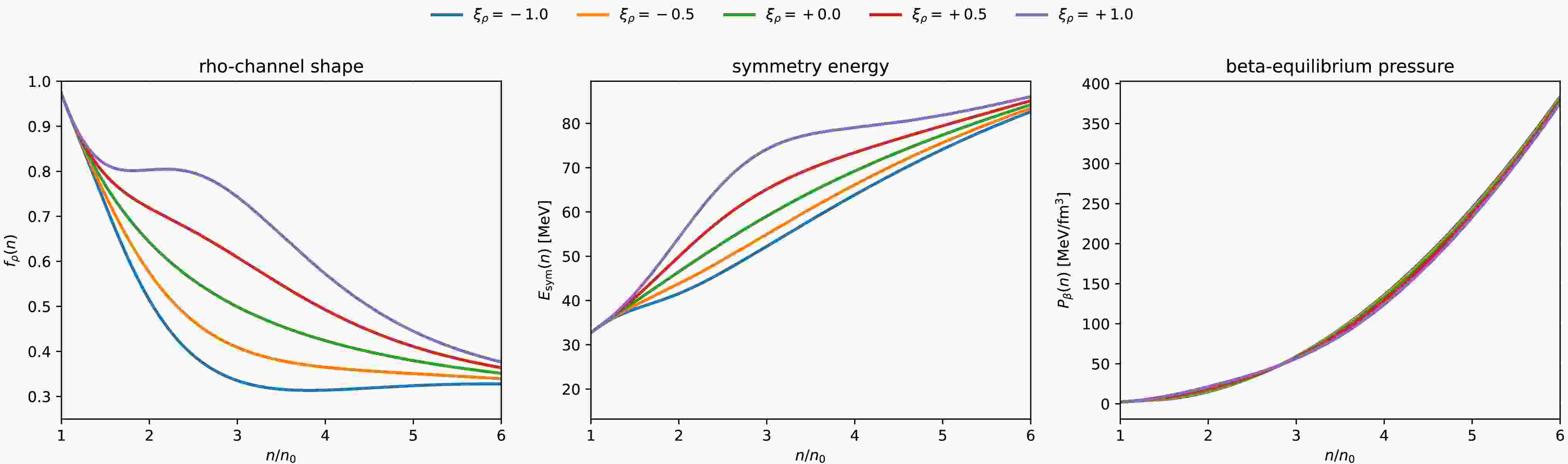
$ {\boldsymbol{\theta}}_{10} $ reproduces these nuclear matter properties and, after the stability and causality filters described below are applied, yields a causal and thermodynamically consistent EOS. The ranges in Table 1 were chosen to be broad enough to encompass the empirical uncertainties of the saturation properties while avoiding parameter regions already incompatible with standard nuclear-matter systematics [24, 44]. The intervals for$ K_0 $ ,$ n_0 $ ,$ E_0 $ ,$ E_{\rm{sym}}(n_0) $ , L, and$ K_{\rm{sym}} $ cover commonly used phenomenological and microscopic constraints around saturation, and the range$ m^*/M=0.45 $ –0.65 spans the relativistic effective masses typically used in covariant density functionals [44, 66]. The three quantities$ f_{\sigma,\infty} $ ,$ f_{\omega,\infty} $ , and$ f_{\rho,\infty} $ are dimensionless asymptotic shape factors rather than coupling constants themselves. Their prior intervals were therefore chosen as wide channel-control ranges, following the inverse-mapped 10D baseline analysis [66]: they allow both softened and stiffened high-density continuations relative to the saturation-normalized value$ f_i(1)=1 $ , while keeping the mapping numerically well conditioned and ensuring that the final EOS is subject to the stability and causality filters. In particular,$ f_{\sigma,\infty} $ controls the high-density scalar attraction,$ f_{\omega,\infty} $ controls the high-density isoscalar-vector repulsion and hence the bulk stiffness, and$ f_{\rho,\infty} $ controls the baseline high-density isovector channel. For the additional 11D parameter we adopt the symmetric prior$ \xi_\rho\in[-1,1] $ . With the fixed deformation width$ \lambda_\rho=1.5 $ , the function$ h(x) $ peaks at$ x=3 $ ; hence, this prior modulates the ρ-channel shape by a moderate multiplicative factor around the density region most relevant for the high-density symmetry energy, proton fraction, and direct-Urca threshold, without modifying the saturation value, slope, curvature, or asymptotic limit of the baseline shape. Larger values of$ |\xi_\rho| $ would cause the posterior to be dominated by artificial prior excursions of the ρ-channel rather than by the data constraints considered here. -
We start from a density-dependent relativistic mean-field model in which nucleons interact through isoscalar-scalar σ, isoscalar-vector ω, and isovector-vector ρ channels. The general form follows the standard covariant density-functional and density-dependent RMF framework [39−45]. In uniform matter, the Lagrangian density may be written schematically as
$ \begin{aligned}[b] {\cal{L}} =&\, \bar{\psi} \left[ \gamma_\mu \left( {\mathrm{i}}\partial^\mu -\Gamma_\omega(n)\omega^\mu -\Gamma_\rho(n)\boldsymbol{\tau}\cdot{\boldsymbol{\rho}}^{\,\mu} \right) -\left(M-\Gamma_\sigma(n)\sigma\right) \right]\psi \\ &+ \frac{1}{2} \left( \partial_\mu\sigma\partial^\mu\sigma -m_\sigma^2\sigma^2 \right) -\frac{1}{4}\omega_{\mu\nu}\omega^{\mu\nu} +\frac{1}{2}m_\omega^2\omega_\mu\omega^\mu \\ &- \frac{1}{4}{\boldsymbol{\rho}}_{\mu\nu}\cdot{\boldsymbol{\rho}}^{\mu\nu} +\frac{1}{2}m_\rho^2{\boldsymbol{\rho}}_\mu\cdot{\boldsymbol{\rho}}^{\mu} +{\cal{L}}_{\rm{lep}}, \end{aligned} $
(1) where M is the nucleon mass, ψ is the nucleon field, and
$ {\cal{L}}_{\rm{lep}} $ denotes the free electron and muon contributions used in beta-equilibrated matter. The density-dependent couplings$ \Gamma_i(n) $ are functions of the baryon density n. It is convenient to introduce the reduced coupling strengths$ G_i(n)=\frac{\Gamma_i^2(n)}{m_i^2}, \qquad i=\sigma,\omega,\rho\, . $
(2) In the TW-like representation used below, each reduced coupling is written as
$ G_i(n)=G_{i0} f_i^2(x), \qquad x=\frac{n}{n_0}, \qquad f_i(1)=1 , $
(3) where
$ G_{i0}=G_i(n_0) $ is the coupling strength at saturation and$ f_i(x) $ is the dimensionless density-dependence function for channel i. The normalization$ f_i(1)=1 $ separates the saturation coupling$ G_{i0} $ from the density-dependent shape$ f_i(x) $ . For the TW-like baseline adopted in this work, the shape functions are taken in the rational form [66].$ f_i^{(10)}(x) = a_i \frac{\left[1+b_i(x+d_i)^2\right]}{\left[1+c_i(x+d_i)^2\right]}, \qquad i=\sigma,\omega,\rho , $
(4) With channel-dependent coefficients
$ a_i,b_i,c_i,d_i $ fixed by the inverse mapping described below, the ten sampled parameters are not themselves the coupling constants; equivalently, they specify the nuclear-matter anchors and high-density limits from which$ G_{i0} $ and the coefficients of$ f_i^{(10)}(x) $ are obtained, as in our recent work [66].In the mean-field approximation for homogeneous matter, only the time components of the vector fields survive. The Dirac effective mass is
$ M^* = M - \Gamma_\sigma(n)\sigma = M - G_\sigma(n)n_s $ , where$ n_s = n_{s,p}+n_{s,n} $ is the total scalar density. The neutron and proton number densities are denoted by$ n_n $ and$ n_p $ , with$ n=n_n+n_p $ and$ n_3=n_p-n_n $ . The energy density of uniform nucleonic matter can be written as$ \epsilon_N = \epsilon_{\rm{kin}}(n_n,n_p,M^*) + \frac{1}{2}G_\sigma(n)n_s^2 + \frac{1}{2}G_\omega(n)n^2 + \frac{1}{2}G_\rho(n)n_3^2 , $
(5) where
$ \epsilon_{\rm{kin}} $ is the sum of the neutron and proton kinetic contributions.Because the couplings are density-dependent, thermodynamic consistency requires the rearrangement self-energy. With the convention used in Eq. (5), the rearrangement contribution is
$ \Sigma_R = \frac{1}{2}\frac{{\rm d}G_\omega}{{\rm d}n}n^2 + \frac{1}{2}\frac{{\rm d}G_\rho}{{\rm d}n}n_3^2 - \frac{1}{2}\frac{{\rm d}G_\sigma}{{\rm d}n}n_s^2 . $
(6) The nucleon chemical potentials are then given by
$ \mu_i = E_{F,i}^* + G_\omega(n)n + t_{3i}G_\rho(n)n_3 + \Sigma_R , \qquad i=n,p , $
(7) where
$ E_{F,i}^*=\sqrt{k_{F,i}^2+M^{*2}} $ , and$ t_{3i} $ denotes the isospin factor. The convention used here is$ n_3=n_p-n_n $ ; thus,$ t_{3p}=+1 $ for protons and$ t_{3n}=-1 $ for neutrons. The pressure is obtained consistently from$ P_N = \sum\limits_{i=n,p}P_{{\rm{kin}},i} - \frac{1}{2}G_\sigma(n)n_s^2 + \frac{1}{2}G_\omega(n)n^2 + \frac{1}{2}G_\rho(n)n_3^2 + n\Sigma_R . $
(8) This expression is equivalent to the thermodynamic identity.
$ P_N=n^2\frac{\partial}{\partial n}\left(\frac{\epsilon_N}{n}\right), $
(9) provided that the rearrangement term is included.
The baseline model employs TW-like density dependence for the meson-nucleon couplings. Instead of fitting the coupling-function parameters directly, we use an inverse-mapping strategy in which the low-density part of the functional is specified by empirical nuclear matter properties at saturation, while the high-density behavior is controlled by asymptotic channel parameters. The 10D parameter vector is given in [66]
$ {\boldsymbol{\theta}}_{10} = \left( K_0, m^*/M, n_0, E_0, E_{\rm{sym}}(n_0), L, K_{\rm{sym}}, f_{\sigma,\infty}, f_{\omega,\infty}, f_{\rho,\infty} \right). $
(10) Here
$ K_0 $ ,$ m^*/M $ ,$ n_0 $ , and$ E_0 $ characterize the isoscalar sector around saturation, while$ E_{\rm{sym}}(n_0) $ , L, and$ K_{\rm{sym}} $ specify the symmetry energy and its first two density derivatives at$ n_0 $ . The three parameters$ f_{\sigma,\infty} $ ,$ f_{\omega,\infty} $ , and$ f_{\rho,\infty} $ control the high-density limits of the corresponding density-dependent channels. The prior ranges used for these parameters are listed in Table 1. The inverse mapping proceeds as follows. First,$ m^*/M $ ,$ n_0 $ , and$ E_0 $ determine the saturation values of the isoscalar reduced couplings$ G_{\sigma0} $ and$ G_{\omega0} $ using the effective-mass relation and the binding energy of symmetric nuclear matter at saturation. Second,$ E_{\rm{sym}}(n_0) $ determines$ G_{\rho0} $ through the symmetry-energy expression given below in Eq. (26). Third, the derivatives required by L,$ K_{\rm{sym}} $ , and$ K_0 $ , together with the imposed asymptotic values.Parameter Prior range Parameter Prior range $ K_0 $ $ [220,260] $ MeV$ K_{\rm{sym}} $ $ [-400,100] $ MeV$ m^*/M $ $ [0.45,0.65] $ $ f_{\sigma,\infty} $ $ [0.3,0.9] $ $ n_0 $ $ [0.145,0.170] $ fm-3$ f_{\omega,\infty} $ $ [0.3,1.4] $ $ E_0 $ $ [-16.5,-15.8] $ MeV$ f_{\rho,\infty} $ $ [0.2,0.9] $ $ E_{\rm{sym}}(n_0) $ $ [28.5,34.9] $ MeV$ \xi_\rho $ $ [-1,1] $ L $ [20,120] $ MeVTable 1. The prior ranges of the model parameters used in the 10D baseline and 11D ρ-flex DD-RMF analyses are presented below. The first ten parameters are common to both models, while
$ \xi_\rho $ is included only in the 11D extension.$ \lim\limits_{x\to\infty} f_i^{(10)}(x)=f_{i,\infty}, \qquad i=\sigma,\omega,\rho , $
(11) This fixes the remaining TW-like shape coefficients. In this way, a sampled point
$ {\boldsymbol{\theta}}_{10} $ uniquely defines the three density-dependent couplings$ G_\sigma(n) $ ,$ G_\omega(n) $ , and$ G_\rho(n) $ , subject to the stability and causality filters used in the Bayesian analysis.The numerical implementation follows this inverse mapping explicitly. At saturation, the chosen effective mass
$ M_0^* = M (m^*/M) $ fixes$ G_{\sigma0}=\frac{M-M_0^*}{n_{s0}}, $
(12) where
$ n_{s0} $ is the scalar density of symmetric matter at$ n_0 $ . The binding energy then fixes the isoscalar-vector coupling through$ G_{\omega0} = \frac{2}{n_0} \left[ M+E_0-\frac{\epsilon_{{\rm{kin}},0}}{n_0} -\frac{1}{2}G_{\sigma0}\frac{n_{s0}^2}{n_0} \right], $
(13) and the saturation symmetry energy fixes
$ G_{\rho0} = \frac{2}{n_0} \left[ E_{\rm{sym}}(n_0)-\frac{k_{F0}^2}{6E_{F0}^*} \right], $
(14) where
$ k_{F0}=(3\pi^2 n_0/2)^{1/3} $ and$ E_{F0}^*=\sqrt{k_{F0}^2+M_0^{*2}} $ . For the ρ channel, the four coefficients of$ f_\rho^{(10)}(x) $ are obtained by solving$ f_\rho(1)=1,\qquad f_\rho(\infty)=f_{\rho,\infty},\qquad \left.\frac{{\mathrm{d}}f_\rho}{{\mathrm{d}}x}\right|_{1}=\eta_\rho,\qquad \left.\frac{{\mathrm{d}}^2f_\rho}{{\mathrm{d}}x^2}\right|_{1}=\kappa_\rho , $
(15) where
$ \eta_\rho $ and$ \kappa_\rho $ are determined from L and$ K_{\rm{sym}} $ after subtracting the kinetic contribution to the symmetry energy. The σ- and ω-channel shapes are then constructed using the same rational form and shift parameter d as the mapped ρ channel. For given$ f_{\sigma,\infty} $ and$ f_{\omega,\infty} $ , their remaining shape parameters are obtained by solving the two symmetric-matter conditions.$ P_{\rm{SNM}}(n_0)=0, \qquad K_{\rm{SNM}}(n_0)=K_0 . $
(16) In practice, these nonlinear equations are solved by a root search with a least-squares fallback. Sampled points for which the mapping fails or for which the resulting EOS violates the stability and causality filters are rejected.
For symmetric nuclear matter (SNM), the saturation point is fixed by
$ \left. \frac{\partial}{\partial n} \left(\frac{\epsilon_{\rm{SNM}}}{n}-M\right) \right|_{n=n_0} =0, \qquad E_0= \left. \left(\frac{\epsilon_{\rm{SNM}}}{n}-M\right) \right|_{n=n_0}. $
(17) The incompressibility is defined as
$ K_0 = 9n_0^2 \left. \frac{\partial^2}{\partial n^2} \left(\frac{\epsilon_{\rm{SNM}}}{n}\right) \right|_{n=n_0}. $
(18) The symmetry energy is obtained from the quadratic expansion of the energy per baryon in the isospin asymmetry
$ \delta=(n_n-n_p)/n $ , namely$ \frac{\epsilon(n,\delta)}{n}-M = E_{\rm{SNM}}(n) + E_{\rm{sym}}(n)\delta^2 + {\cal{O}}(\delta^4). $
(19) Its slope and curvature at saturation are
$ L = 3n_0 \left. \frac{\partial E_{\rm{sym}}(n)}{\partial n} \right|_{n=n_0}, \qquad K_{\rm{sym}} = 9n_0^2 \left. \frac{\partial^2 E_{\rm{sym}}(n)}{\partial n^2} \right|_{n=n_0}. $
(20) The inverse mapping determines the density-dependent couplings such that the chosen parameter set
$ {\boldsymbol{\theta}}_{10} $ reproduces these nuclear matter properties and, after the stability and causality filters described below are applied, yields a causal and thermodynamically consistent EOS. The ranges in Table 1 were chosen to be broad enough to encompass the empirical uncertainties of the saturation properties while avoiding parameter regions already incompatible with standard nuclear-matter systematics [24, 44]. The intervals for$ K_0 $ ,$ n_0 $ ,$ E_0 $ ,$ E_{\rm{sym}}(n_0) $ , L, and$ K_{\rm{sym}} $ cover commonly used phenomenological and microscopic constraints around saturation, and the range$ m^*/M=0.45 $ –0.65 spans the relativistic effective masses typically used in covariant density functionals [44, 66]. The three quantities$ f_{\sigma,\infty} $ ,$ f_{\omega,\infty} $ , and$ f_{\rho,\infty} $ are dimensionless asymptotic shape factors rather than coupling constants themselves. Their prior intervals were therefore chosen as wide channel-control ranges, following the inverse-mapped 10D baseline analysis [66]: they allow both softened and stiffened high-density continuations relative to the saturation-normalized value$ f_i(1)=1 $ , while keeping the mapping numerically well conditioned and ensuring that the final EOS is subject to the stability and causality filters. In particular,$ f_{\sigma,\infty} $ controls the high-density scalar attraction,$ f_{\omega,\infty} $ controls the high-density isoscalar-vector repulsion and hence the bulk stiffness, and$ f_{\rho,\infty} $ controls the baseline high-density isovector channel. For the additional 11D parameter we adopt the symmetric prior$ \xi_\rho\in[-1,1] $ . With the fixed deformation width$ \lambda_\rho=1.5 $ , the function$ h(x) $ peaks at$ x=3 $ ; hence, this prior modulates the ρ-channel shape by a moderate multiplicative factor around the density region most relevant for the high-density symmetry energy, proton fraction, and direct-Urca threshold, without modifying the saturation value, slope, curvature, or asymptotic limit of the baseline shape. Larger values of$ |\xi_\rho| $ would cause the posterior to be dominated by artificial prior excursions of the ρ-channel rather than by the data constraints considered here. -
We start from a density-dependent relativistic mean-field model in which nucleons interact through isoscalar-scalar σ, isoscalar-vector ω, and isovector-vector ρ channels. The general form follows the standard covariant density-functional and density-dependent RMF framework [39−45]. In uniform matter, the Lagrangian density may be written schematically as
$ \begin{aligned}[b] {\cal{L}} =&\, \bar{\psi} \left[ \gamma_\mu \left( {\mathrm{i}}\partial^\mu -\Gamma_\omega(n)\omega^\mu -\Gamma_\rho(n)\boldsymbol{\tau}\cdot{\boldsymbol{\rho}}^{\,\mu} \right) -\left(M-\Gamma_\sigma(n)\sigma\right) \right]\psi \\ &+ \frac{1}{2} \left( \partial_\mu\sigma\partial^\mu\sigma -m_\sigma^2\sigma^2 \right) -\frac{1}{4}\omega_{\mu\nu}\omega^{\mu\nu} +\frac{1}{2}m_\omega^2\omega_\mu\omega^\mu \\ &- \frac{1}{4}{\boldsymbol{\rho}}_{\mu\nu}\cdot{\boldsymbol{\rho}}^{\mu\nu} +\frac{1}{2}m_\rho^2{\boldsymbol{\rho}}_\mu\cdot{\boldsymbol{\rho}}^{\mu} +{\cal{L}}_{\rm{lep}}, \end{aligned} $
(1) where M is the nucleon mass, ψ is the nucleon field, and
$ {\cal{L}}_{\rm{lep}} $ denotes the free electron and muon contributions used in beta-equilibrated matter. The density-dependent couplings$ \Gamma_i(n) $ are functions of the baryon density n. It is convenient to introduce the reduced coupling strengths$ G_i(n)=\frac{\Gamma_i^2(n)}{m_i^2}, \qquad i=\sigma,\omega,\rho\, . $
(2) In the TW-like representation used below, each reduced coupling is written as
$ G_i(n)=G_{i0} f_i^2(x), \qquad x=\frac{n}{n_0}, \qquad f_i(1)=1 , $
(3) where
$ G_{i0}=G_i(n_0) $ is the coupling strength at saturation and$ f_i(x) $ is the dimensionless density-dependence function for channel i. The normalization$ f_i(1)=1 $ separates the saturation coupling$ G_{i0} $ from the density-dependent shape$ f_i(x) $ . For the TW-like baseline adopted in this work, the shape functions are taken in the rational form [66].$ f_i^{(10)}(x) = a_i \frac{\left[1+b_i(x+d_i)^2\right]}{\left[1+c_i(x+d_i)^2\right]}, \qquad i=\sigma,\omega,\rho , $
(4) With channel-dependent coefficients
$ a_i,b_i,c_i,d_i $ fixed by the inverse mapping described below, the ten sampled parameters are not themselves the coupling constants; equivalently, they specify the nuclear-matter anchors and high-density limits from which$ G_{i0} $ and the coefficients of$ f_i^{(10)}(x) $ are obtained, as in our recent work [66].In the mean-field approximation for homogeneous matter, only the time components of the vector fields survive. The Dirac effective mass is
$ M^* = M - \Gamma_\sigma(n)\sigma = M - G_\sigma(n)n_s $ , where$ n_s = n_{s,p}+n_{s,n} $ is the total scalar density. The neutron and proton number densities are denoted by$ n_n $ and$ n_p $ , with$ n=n_n+n_p $ and$ n_3=n_p-n_n $ . The energy density of uniform nucleonic matter can be written as$ \epsilon_N = \epsilon_{\rm{kin}}(n_n,n_p,M^*) + \frac{1}{2}G_\sigma(n)n_s^2 + \frac{1}{2}G_\omega(n)n^2 + \frac{1}{2}G_\rho(n)n_3^2 , $
(5) where
$ \epsilon_{\rm{kin}} $ is the sum of the neutron and proton kinetic contributions.Because the couplings are density-dependent, thermodynamic consistency requires the rearrangement self-energy. With the convention used in Eq. (5), the rearrangement contribution is
$ \Sigma_R = \frac{1}{2}\frac{{\rm d}G_\omega}{{\rm d}n}n^2 + \frac{1}{2}\frac{{\rm d}G_\rho}{{\rm d}n}n_3^2 - \frac{1}{2}\frac{{\rm d}G_\sigma}{{\rm d}n}n_s^2 . $
(6) The nucleon chemical potentials are then given by
$ \mu_i = E_{F,i}^* + G_\omega(n)n + t_{3i}G_\rho(n)n_3 + \Sigma_R , \qquad i=n,p , $
(7) where
$ E_{F,i}^*=\sqrt{k_{F,i}^2+M^{*2}} $ , and$ t_{3i} $ denotes the isospin factor. The convention used here is$ n_3=n_p-n_n $ ; thus,$ t_{3p}=+1 $ for protons and$ t_{3n}=-1 $ for neutrons. The pressure is obtained consistently from$ P_N = \sum\limits_{i=n,p}P_{{\rm{kin}},i} - \frac{1}{2}G_\sigma(n)n_s^2 + \frac{1}{2}G_\omega(n)n^2 + \frac{1}{2}G_\rho(n)n_3^2 + n\Sigma_R . $
(8) This expression is equivalent to the thermodynamic identity.
$ P_N=n^2\frac{\partial}{\partial n}\left(\frac{\epsilon_N}{n}\right), $
(9) provided that the rearrangement term is included.
The baseline model employs TW-like density dependence for the meson-nucleon couplings. Instead of fitting the coupling-function parameters directly, we use an inverse-mapping strategy in which the low-density part of the functional is specified by empirical nuclear matter properties at saturation, while the high-density behavior is controlled by asymptotic channel parameters. The 10D parameter vector is given in [66]
$ {\boldsymbol{\theta}}_{10} = \left( K_0, m^*/M, n_0, E_0, E_{\rm{sym}}(n_0), L, K_{\rm{sym}}, f_{\sigma,\infty}, f_{\omega,\infty}, f_{\rho,\infty} \right). $
(10) Here
$ K_0 $ ,$ m^*/M $ ,$ n_0 $ , and$ E_0 $ characterize the isoscalar sector around saturation, while$ E_{\rm{sym}}(n_0) $ , L, and$ K_{\rm{sym}} $ specify the symmetry energy and its first two density derivatives at$ n_0 $ . The three parameters$ f_{\sigma,\infty} $ ,$ f_{\omega,\infty} $ , and$ f_{\rho,\infty} $ control the high-density limits of the corresponding density-dependent channels. The prior ranges used for these parameters are listed in Table 1. The inverse mapping proceeds as follows. First,$ m^*/M $ ,$ n_0 $ , and$ E_0 $ determine the saturation values of the isoscalar reduced couplings$ G_{\sigma0} $ and$ G_{\omega0} $ using the effective-mass relation and the binding energy of symmetric nuclear matter at saturation. Second,$ E_{\rm{sym}}(n_0) $ determines$ G_{\rho0} $ through the symmetry-energy expression given below in Eq. (26). Third, the derivatives required by L,$ K_{\rm{sym}} $ , and$ K_0 $ , together with the imposed asymptotic values.Parameter Prior range Parameter Prior range $ K_0 $ $ [220,260] $ MeV$ K_{\rm{sym}} $ $ [-400,100] $ MeV$ m^*/M $ $ [0.45,0.65] $ $ f_{\sigma,\infty} $ $ [0.3,0.9] $ $ n_0 $ $ [0.145,0.170] $ fm-3$ f_{\omega,\infty} $ $ [0.3,1.4] $ $ E_0 $ $ [-16.5,-15.8] $ MeV$ f_{\rho,\infty} $ $ [0.2,0.9] $ $ E_{\rm{sym}}(n_0) $ $ [28.5,34.9] $ MeV$ \xi_\rho $ $ [-1,1] $ L $ [20,120] $ MeVTable 1. The prior ranges of the model parameters used in the 10D baseline and 11D ρ-flex DD-RMF analyses are presented below. The first ten parameters are common to both models, while
$ \xi_\rho $ is included only in the 11D extension.$ \lim\limits_{x\to\infty} f_i^{(10)}(x)=f_{i,\infty}, \qquad i=\sigma,\omega,\rho , $
(11) This fixes the remaining TW-like shape coefficients. In this way, a sampled point
$ {\boldsymbol{\theta}}_{10} $ uniquely defines the three density-dependent couplings$ G_\sigma(n) $ ,$ G_\omega(n) $ , and$ G_\rho(n) $ , subject to the stability and causality filters used in the Bayesian analysis.The numerical implementation follows this inverse mapping explicitly. At saturation, the chosen effective mass
$ M_0^* = M (m^*/M) $ fixes$ G_{\sigma0}=\frac{M-M_0^*}{n_{s0}}, $
(12) where
$ n_{s0} $ is the scalar density of symmetric matter at$ n_0 $ . The binding energy then fixes the isoscalar-vector coupling through$ G_{\omega0} = \frac{2}{n_0} \left[ M+E_0-\frac{\epsilon_{{\rm{kin}},0}}{n_0} -\frac{1}{2}G_{\sigma0}\frac{n_{s0}^2}{n_0} \right], $
(13) and the saturation symmetry energy fixes
$ G_{\rho0} = \frac{2}{n_0} \left[ E_{\rm{sym}}(n_0)-\frac{k_{F0}^2}{6E_{F0}^*} \right], $
(14) where
$ k_{F0}=(3\pi^2 n_0/2)^{1/3} $ and$ E_{F0}^*=\sqrt{k_{F0}^2+M_0^{*2}} $ . For the ρ channel, the four coefficients of$ f_\rho^{(10)}(x) $ are obtained by solving$ f_\rho(1)=1,\qquad f_\rho(\infty)=f_{\rho,\infty},\qquad \left.\frac{{\mathrm{d}}f_\rho}{{\mathrm{d}}x}\right|_{1}=\eta_\rho,\qquad \left.\frac{{\mathrm{d}}^2f_\rho}{{\mathrm{d}}x^2}\right|_{1}=\kappa_\rho , $
(15) where
$ \eta_\rho $ and$ \kappa_\rho $ are determined from L and$ K_{\rm{sym}} $ after subtracting the kinetic contribution to the symmetry energy. The σ- and ω-channel shapes are then constructed using the same rational form and shift parameter d as the mapped ρ channel. For given$ f_{\sigma,\infty} $ and$ f_{\omega,\infty} $ , their remaining shape parameters are obtained by solving the two symmetric-matter conditions.$ P_{\rm{SNM}}(n_0)=0, \qquad K_{\rm{SNM}}(n_0)=K_0 . $
(16) In practice, these nonlinear equations are solved by a root search with a least-squares fallback. Sampled points for which the mapping fails or for which the resulting EOS violates the stability and causality filters are rejected.
For symmetric nuclear matter (SNM), the saturation point is fixed by
$ \left. \frac{\partial}{\partial n} \left(\frac{\epsilon_{\rm{SNM}}}{n}-M\right) \right|_{n=n_0} =0, \qquad E_0= \left. \left(\frac{\epsilon_{\rm{SNM}}}{n}-M\right) \right|_{n=n_0}. $
(17) The incompressibility is defined as
$ K_0 = 9n_0^2 \left. \frac{\partial^2}{\partial n^2} \left(\frac{\epsilon_{\rm{SNM}}}{n}\right) \right|_{n=n_0}. $
(18) The symmetry energy is obtained from the quadratic expansion of the energy per baryon in the isospin asymmetry
$ \delta=(n_n-n_p)/n $ , namely$ \frac{\epsilon(n,\delta)}{n}-M = E_{\rm{SNM}}(n) + E_{\rm{sym}}(n)\delta^2 + {\cal{O}}(\delta^4). $
(19) Its slope and curvature at saturation are
$ L = 3n_0 \left. \frac{\partial E_{\rm{sym}}(n)}{\partial n} \right|_{n=n_0}, \qquad K_{\rm{sym}} = 9n_0^2 \left. \frac{\partial^2 E_{\rm{sym}}(n)}{\partial n^2} \right|_{n=n_0}. $
(20) The inverse mapping determines the density-dependent couplings such that the chosen parameter set
$ {\boldsymbol{\theta}}_{10} $ reproduces these nuclear matter properties and, after the stability and causality filters described below are applied, yields a causal and thermodynamically consistent EOS. The ranges in Table 1 were chosen to be broad enough to encompass the empirical uncertainties of the saturation properties while avoiding parameter regions already incompatible with standard nuclear-matter systematics [24, 44]. The intervals for$ K_0 $ ,$ n_0 $ ,$ E_0 $ ,$ E_{\rm{sym}}(n_0) $ , L, and$ K_{\rm{sym}} $ cover commonly used phenomenological and microscopic constraints around saturation, and the range$ m^*/M=0.45 $ –0.65 spans the relativistic effective masses typically used in covariant density functionals [44, 66]. The three quantities$ f_{\sigma,\infty} $ ,$ f_{\omega,\infty} $ , and$ f_{\rho,\infty} $ are dimensionless asymptotic shape factors rather than coupling constants themselves. Their prior intervals were therefore chosen as wide channel-control ranges, following the inverse-mapped 10D baseline analysis [66]: they allow both softened and stiffened high-density continuations relative to the saturation-normalized value$ f_i(1)=1 $ , while keeping the mapping numerically well conditioned and ensuring that the final EOS is subject to the stability and causality filters. In particular,$ f_{\sigma,\infty} $ controls the high-density scalar attraction,$ f_{\omega,\infty} $ controls the high-density isoscalar-vector repulsion and hence the bulk stiffness, and$ f_{\rho,\infty} $ controls the baseline high-density isovector channel. For the additional 11D parameter we adopt the symmetric prior$ \xi_\rho\in[-1,1] $ . With the fixed deformation width$ \lambda_\rho=1.5 $ , the function$ h(x) $ peaks at$ x=3 $ ; hence, this prior modulates the ρ-channel shape by a moderate multiplicative factor around the density region most relevant for the high-density symmetry energy, proton fraction, and direct-Urca threshold, without modifying the saturation value, slope, curvature, or asymptotic limit of the baseline shape. Larger values of$ |\xi_\rho| $ would cause the posterior to be dominated by artificial prior excursions of the ρ-channel rather than by the data constraints considered here. -
We start from a density-dependent relativistic mean-field model in which nucleons interact through isoscalar-scalar σ, isoscalar-vector ω, and isovector-vector ρ channels. The general form follows the standard covariant density-functional and density-dependent RMF framework [39−45]. In uniform matter, the Lagrangian density may be written schematically as
$ \begin{aligned}[b] {\cal{L}} =&\, \bar{\psi} \left[ \gamma_\mu \left( {\mathrm{i}}\partial^\mu -\Gamma_\omega(n)\omega^\mu -\Gamma_\rho(n)\boldsymbol{\tau}\cdot{\boldsymbol{\rho}}^{\,\mu} \right) -\left(M-\Gamma_\sigma(n)\sigma\right) \right]\psi \\ &+ \frac{1}{2} \left( \partial_\mu\sigma\partial^\mu\sigma -m_\sigma^2\sigma^2 \right) -\frac{1}{4}\omega_{\mu\nu}\omega^{\mu\nu} +\frac{1}{2}m_\omega^2\omega_\mu\omega^\mu \\ &- \frac{1}{4}{\boldsymbol{\rho}}_{\mu\nu}\cdot{\boldsymbol{\rho}}^{\mu\nu} +\frac{1}{2}m_\rho^2{\boldsymbol{\rho}}_\mu\cdot{\boldsymbol{\rho}}^{\mu} +{\cal{L}}_{\rm{lep}}, \end{aligned} $
(1) where M is the nucleon mass, ψ is the nucleon field, and
$ {\cal{L}}_{\rm{lep}} $ denotes the free electron and muon contributions used in beta-equilibrated matter. The density-dependent couplings$ \Gamma_i(n) $ are functions of the baryon density n. It is convenient to introduce the reduced coupling strengths$ G_i(n)=\frac{\Gamma_i^2(n)}{m_i^2}, \qquad i=\sigma,\omega,\rho\, . $
(2) In the TW-like representation used below, each reduced coupling is written as
$ G_i(n)=G_{i0} f_i^2(x), \qquad x=\frac{n}{n_0}, \qquad f_i(1)=1 , $
(3) where
$ G_{i0}=G_i(n_0) $ is the coupling strength at saturation and$ f_i(x) $ is the dimensionless density-dependence function for channel i. The normalization$ f_i(1)=1 $ separates the saturation coupling$ G_{i0} $ from the density-dependent shape$ f_i(x) $ . For the TW-like baseline adopted in this work, the shape functions are taken in the rational form [66].$ f_i^{(10)}(x) = a_i \frac{\left[1+b_i(x+d_i)^2\right]}{\left[1+c_i(x+d_i)^2\right]}, \qquad i=\sigma,\omega,\rho , $
(4) With channel-dependent coefficients
$ a_i,b_i,c_i,d_i $ fixed by the inverse mapping described below, the ten sampled parameters are not themselves the coupling constants; equivalently, they specify the nuclear-matter anchors and high-density limits from which$ G_{i0} $ and the coefficients of$ f_i^{(10)}(x) $ are obtained, as in our recent work [66].In the mean-field approximation for homogeneous matter, only the time components of the vector fields survive. The Dirac effective mass is
$ M^* = M - \Gamma_\sigma(n)\sigma = M - G_\sigma(n)n_s $ , where$ n_s = n_{s,p}+n_{s,n} $ is the total scalar density. The neutron and proton number densities are denoted by$ n_n $ and$ n_p $ , with$ n=n_n+n_p $ and$ n_3=n_p-n_n $ . The energy density of uniform nucleonic matter can be written as$ \epsilon_N = \epsilon_{\rm{kin}}(n_n,n_p,M^*) + \frac{1}{2}G_\sigma(n)n_s^2 + \frac{1}{2}G_\omega(n)n^2 + \frac{1}{2}G_\rho(n)n_3^2 , $
(5) where
$ \epsilon_{\rm{kin}} $ is the sum of the neutron and proton kinetic contributions.Because the couplings are density-dependent, thermodynamic consistency requires the rearrangement self-energy. With the convention used in Eq. (5), the rearrangement contribution is
$ \Sigma_R = \frac{1}{2}\frac{{\rm d}G_\omega}{{\rm d}n}n^2 + \frac{1}{2}\frac{{\rm d}G_\rho}{{\rm d}n}n_3^2 - \frac{1}{2}\frac{{\rm d}G_\sigma}{{\rm d}n}n_s^2 . $
(6) The nucleon chemical potentials are then given by
$ \mu_i = E_{F,i}^* + G_\omega(n)n + t_{3i}G_\rho(n)n_3 + \Sigma_R , \qquad i=n,p , $
(7) where
$ E_{F,i}^*=\sqrt{k_{F,i}^2+M^{*2}} $ , and$ t_{3i} $ denotes the isospin factor. The convention used here is$ n_3=n_p-n_n $ ; thus,$ t_{3p}=+1 $ for protons and$ t_{3n}=-1 $ for neutrons. The pressure is obtained consistently from$ P_N = \sum\limits_{i=n,p}P_{{\rm{kin}},i} - \frac{1}{2}G_\sigma(n)n_s^2 + \frac{1}{2}G_\omega(n)n^2 + \frac{1}{2}G_\rho(n)n_3^2 + n\Sigma_R . $
(8) This expression is equivalent to the thermodynamic identity.
$ P_N=n^2\frac{\partial}{\partial n}\left(\frac{\epsilon_N}{n}\right), $
(9) provided that the rearrangement term is included.
The baseline model employs TW-like density dependence for the meson-nucleon couplings. Instead of fitting the coupling-function parameters directly, we use an inverse-mapping strategy in which the low-density part of the functional is specified by empirical nuclear matter properties at saturation, while the high-density behavior is controlled by asymptotic channel parameters. The 10D parameter vector is given in [66]
$ {\boldsymbol{\theta}}_{10} = \left( K_0, m^*/M, n_0, E_0, E_{\rm{sym}}(n_0), L, K_{\rm{sym}}, f_{\sigma,\infty}, f_{\omega,\infty}, f_{\rho,\infty} \right). $
(10) Here
$ K_0 $ ,$ m^*/M $ ,$ n_0 $ , and$ E_0 $ characterize the isoscalar sector around saturation, while$ E_{\rm{sym}}(n_0) $ , L, and$ K_{\rm{sym}} $ specify the symmetry energy and its first two density derivatives at$ n_0 $ . The three parameters$ f_{\sigma,\infty} $ ,$ f_{\omega,\infty} $ , and$ f_{\rho,\infty} $ control the high-density limits of the corresponding density-dependent channels. The prior ranges used for these parameters are listed in Table 1. The inverse mapping proceeds as follows. First,$ m^*/M $ ,$ n_0 $ , and$ E_0 $ determine the saturation values of the isoscalar reduced couplings$ G_{\sigma0} $ and$ G_{\omega0} $ using the effective-mass relation and the binding energy of symmetric nuclear matter at saturation. Second,$ E_{\rm{sym}}(n_0) $ determines$ G_{\rho0} $ through the symmetry-energy expression given below in Eq. (26). Third, the derivatives required by L,$ K_{\rm{sym}} $ , and$ K_0 $ , together with the imposed asymptotic values.Parameter Prior range Parameter Prior range $ K_0 $ $ [220,260] $ MeV$ K_{\rm{sym}} $ $ [-400,100] $ MeV$ m^*/M $ $ [0.45,0.65] $ $ f_{\sigma,\infty} $ $ [0.3,0.9] $ $ n_0 $ $ [0.145,0.170] $ fm-3$ f_{\omega,\infty} $ $ [0.3,1.4] $ $ E_0 $ $ [-16.5,-15.8] $ MeV$ f_{\rho,\infty} $ $ [0.2,0.9] $ $ E_{\rm{sym}}(n_0) $ $ [28.5,34.9] $ MeV$ \xi_\rho $ $ [-1,1] $ L $ [20,120] $ MeVTable 1. The prior ranges of the model parameters used in the 10D baseline and 11D ρ-flex DD-RMF analyses are presented below. The first ten parameters are common to both models, while
$ \xi_\rho $ is included only in the 11D extension.$ \lim\limits_{x\to\infty} f_i^{(10)}(x)=f_{i,\infty}, \qquad i=\sigma,\omega,\rho , $
(11) This fixes the remaining TW-like shape coefficients. In this way, a sampled point
$ {\boldsymbol{\theta}}_{10} $ uniquely defines the three density-dependent couplings$ G_\sigma(n) $ ,$ G_\omega(n) $ , and$ G_\rho(n) $ , subject to the stability and causality filters used in the Bayesian analysis.The numerical implementation follows this inverse mapping explicitly. At saturation, the chosen effective mass
$ M_0^* = M (m^*/M) $ fixes$ G_{\sigma0}=\frac{M-M_0^*}{n_{s0}}, $
(12) where
$ n_{s0} $ is the scalar density of symmetric matter at$ n_0 $ . The binding energy then fixes the isoscalar-vector coupling through$ G_{\omega0} = \frac{2}{n_0} \left[ M+E_0-\frac{\epsilon_{{\rm{kin}},0}}{n_0} -\frac{1}{2}G_{\sigma0}\frac{n_{s0}^2}{n_0} \right], $
(13) and the saturation symmetry energy fixes
$ G_{\rho0} = \frac{2}{n_0} \left[ E_{\rm{sym}}(n_0)-\frac{k_{F0}^2}{6E_{F0}^*} \right], $
(14) where
$ k_{F0}=(3\pi^2 n_0/2)^{1/3} $ and$ E_{F0}^*=\sqrt{k_{F0}^2+M_0^{*2}} $ . For the ρ channel, the four coefficients of$ f_\rho^{(10)}(x) $ are obtained by solving$ f_\rho(1)=1,\qquad f_\rho(\infty)=f_{\rho,\infty},\qquad \left.\frac{{\mathrm{d}}f_\rho}{{\mathrm{d}}x}\right|_{1}=\eta_\rho,\qquad \left.\frac{{\mathrm{d}}^2f_\rho}{{\mathrm{d}}x^2}\right|_{1}=\kappa_\rho , $
(15) where
$ \eta_\rho $ and$ \kappa_\rho $ are determined from L and$ K_{\rm{sym}} $ after subtracting the kinetic contribution to the symmetry energy. The σ- and ω-channel shapes are then constructed using the same rational form and shift parameter d as the mapped ρ channel. For given$ f_{\sigma,\infty} $ and$ f_{\omega,\infty} $ , their remaining shape parameters are obtained by solving the two symmetric-matter conditions.$ P_{\rm{SNM}}(n_0)=0, \qquad K_{\rm{SNM}}(n_0)=K_0 . $
(16) In practice, these nonlinear equations are solved by a root search with a least-squares fallback. Sampled points for which the mapping fails or for which the resulting EOS violates the stability and causality filters are rejected.
For symmetric nuclear matter (SNM), the saturation point is fixed by
$ \left. \frac{\partial}{\partial n} \left(\frac{\epsilon_{\rm{SNM}}}{n}-M\right) \right|_{n=n_0} =0, \qquad E_0= \left. \left(\frac{\epsilon_{\rm{SNM}}}{n}-M\right) \right|_{n=n_0}. $
(17) The incompressibility is defined as
$ K_0 = 9n_0^2 \left. \frac{\partial^2}{\partial n^2} \left(\frac{\epsilon_{\rm{SNM}}}{n}\right) \right|_{n=n_0}. $
(18) The symmetry energy is obtained from the quadratic expansion of the energy per baryon in the isospin asymmetry
$ \delta=(n_n-n_p)/n $ , namely$ \frac{\epsilon(n,\delta)}{n}-M = E_{\rm{SNM}}(n) + E_{\rm{sym}}(n)\delta^2 + {\cal{O}}(\delta^4). $
(19) Its slope and curvature at saturation are
$ L = 3n_0 \left. \frac{\partial E_{\rm{sym}}(n)}{\partial n} \right|_{n=n_0}, \qquad K_{\rm{sym}} = 9n_0^2 \left. \frac{\partial^2 E_{\rm{sym}}(n)}{\partial n^2} \right|_{n=n_0}. $
(20) The inverse mapping determines the density-dependent couplings such that the chosen parameter set
$ {\boldsymbol{\theta}}_{10} $ reproduces these nuclear matter properties and, after the stability and causality filters described below are applied, yields a causal and thermodynamically consistent EOS. The ranges in Table 1 were chosen to be broad enough to encompass the empirical uncertainties of the saturation properties while avoiding parameter regions already incompatible with standard nuclear-matter systematics [24, 44]. The intervals for$ K_0 $ ,$ n_0 $ ,$ E_0 $ ,$ E_{\rm{sym}}(n_0) $ , L, and$ K_{\rm{sym}} $ cover commonly used phenomenological and microscopic constraints around saturation, and the range$ m^*/M=0.45 $ –0.65 spans the relativistic effective masses typically used in covariant density functionals [44, 66]. The three quantities$ f_{\sigma,\infty} $ ,$ f_{\omega,\infty} $ , and$ f_{\rho,\infty} $ are dimensionless asymptotic shape factors rather than coupling constants themselves. Their prior intervals were therefore chosen as wide channel-control ranges, following the inverse-mapped 10D baseline analysis [66]: they allow both softened and stiffened high-density continuations relative to the saturation-normalized value$ f_i(1)=1 $ , while keeping the mapping numerically well conditioned and ensuring that the final EOS is subject to the stability and causality filters. In particular,$ f_{\sigma,\infty} $ controls the high-density scalar attraction,$ f_{\omega,\infty} $ controls the high-density isoscalar-vector repulsion and hence the bulk stiffness, and$ f_{\rho,\infty} $ controls the baseline high-density isovector channel. For the additional 11D parameter we adopt the symmetric prior$ \xi_\rho\in[-1,1] $ . With the fixed deformation width$ \lambda_\rho=1.5 $ , the function$ h(x) $ peaks at$ x=3 $ ; hence, this prior modulates the ρ-channel shape by a moderate multiplicative factor around the density region most relevant for the high-density symmetry energy, proton fraction, and direct-Urca threshold, without modifying the saturation value, slope, curvature, or asymptotic limit of the baseline shape. Larger values of$ |\xi_\rho| $ would cause the posterior to be dominated by artificial prior excursions of the ρ-channel rather than by the data constraints considered here. -
In the 10D baseline, the density dependence of the isovector ρ-channel is fixed once the saturation-point isovector quantities
$ E_{\rm{sym}}(n_0) $ , L,$ K_{\rm{sym}} $ , and the high-density control parameter$ f_{\rho,\infty} $ are specified. This density-dependent construction follows the standard TW-like DD-RMF framework [41, 44, 45, 49, 66]. Although this parametrization is economical, it may restrict the high-density extrapolation of the symmetry energy. This is relevant because current neutron-star and multimessenger constraints mainly restrict the bulk stiffness of beta-equilibrated matter, while the isovector sector at high densities remains less directly constrained [19, 20, 28, 29, 51, 52]. To quantify this residual model dependence, we introduce an 11D extension in which the ρ-channel is allowed to vary through one additional parameter,$ \xi_\rho $ . The parameter vector is$ {\boldsymbol{\theta}}_{11} = \left( {\boldsymbol{\theta}}_{10}, \xi_\rho \right). $
(21) In the nested limit
$ \xi_\rho=0 $ , the 10D baseline is recovered. The extension is applied only to the isovector channel. The density dependences of the isoscalar σ and ω channels are kept identical to those of the 10D baseline. Thus, in the notation of Eq. (3), the 11D model changes only$ f_\rho(x) $ , whereas$ G_{\sigma0} $ ,$ G_{\omega0} $ ,$ G_{\rho0} $ ,$ f_\sigma^{(10)}(x) $ , and$ f_\omega^{(10)}(x) $ are inherited from the corresponding 10D mapped point.The 11D ρ-channel shape function is written as
$ f_\rho^{(11)}(x) = f_\rho^{(10)}(x) \exp\left[\xi_\rho h(x)\right], \qquad x=\frac{n}{n_0}, $
(22) where
$ f_\rho^{(10)}(x) $ is the TW-like baseline shape for the ρ channel. The deformation function is chosen as$ h(x) = (x-1)^3 \exp\left[-\lambda_\rho(x-1)\right] \Theta(x-1). $
(23) This term is not part of the original 10D baseline parametrization. It is introduced only in the 11D ρ-flex extension as a localized suprasaturation deformation. For the calculations in this work, the width parameter is fixed to
$ \lambda_\rho=1.5 $ , and this value is treated as a hyperparameter rather than as an additional sampled parameter. With this choice, the function$ h(x) $ reaches its maximum at$ x_{\max}=1+3/\lambda_\rho=3 $ , so that the deformation is centered around$ n\simeq 3n_0 $ , a density region relevant for neutron-star radii, proton fractions, and direct Urca thresholds. The value$ \lambda_\rho=1.5 $ is not intended to represent a uniquely preferred physical scale. It defines a compact one-parameter basis deformation that turns on only above saturation, preserves the saturation-point matching conditions, and probes the intermediate-to-high-density interval where the isovector channel is only weakly constrained by present data. Changing$ \lambda_\rho $ would shift the maximum according to$ x_{\max}=1+3/\lambda_\rho $ : a smaller value would move the deformation to higher densities, while a larger value would move it to lower densities. The quantitative posterior intervals reported below should therefore be understood as conditional on this fixed ρ-flex basis. The qualitative diagnostic conclusion, however, is not tied to the precise value of the peak position: the additional ρ-channel freedom mainly affects composition-sensitive quantities such as$ E_{\rm{sym}}(n) $ ,$ Y_p(n) $ , and the direct Urca threshold, whereas the bulk mass–radius and tidal observables are much less sensitive.The functional form in Eq. (23) satisfies
$ h(1)=h'(1)=h''(1)=0, \qquad \lim\limits_{x\rightarrow \infty}h(x)=0. $
(24) Thus, the value, first derivative, and second derivative of the ρ-channel shape at saturation are unaffected by
$ \xi_\rho $ . The asymptotic value$ f_{\rho,\infty} $ is also preserved. Consequently, the saturation-point isovector inputs$ E_{\rm{sym}}(n_0) $ , L,$ K_{\rm{sym}} $ , and the high-density limiting parameter$ f_{\rho,\infty} $ retain their definitions in the 10D and 11D models. The corresponding ρ-channel coupling is$ G_\rho^{(11)}(n) = G_{\rho0} \left[ f_\rho^{(11)}\left(\frac{n}{n_0}\right) \right]^2 . $
(25) The symmetry energy in the parabolic approximation is
$ E_{\rm{sym}}(n) = \frac{k_F^2}{6E_F^*} + \frac{1}{2}G_\rho(n)n , $
(26) where
$ k_F=\left(3\pi^2 n/2\right)^{1/3}, E_F^*=\sqrt{k_F^2+M^{*2}} $ . The first term in Eq. (26) is the kinetic contribution, while the second term is the ρ-channel contribution. Thus,$ \xi_\rho $ changes the high-density symmetry energy by modifying$ G_\rho(n) $ above saturation without changing the imposed saturation-point quantities. The parameter$ \xi_\rho $ should not be interpreted as a new empirical nuclear-matter coefficient. Rather, it is a diagnostic parameter used to test the sensitivity of high-density isovector and composition-sensitive predictions to the assumed ρ-channel density dependence. The prior range adopted in the Bayesian analysis is$ \xi_\rho\in[-1,1] $ , as listed in Table 1. For the 10D baseline calculations, the same formalism is used with$ \xi_\rho $ fixed to zero. -
In the 10D baseline, the density dependence of the isovector ρ-channel is fixed once the saturation-point isovector quantities
$ E_{\rm{sym}}(n_0) $ , L,$ K_{\rm{sym}} $ , and the high-density control parameter$ f_{\rho,\infty} $ are specified. This density-dependent construction follows the standard TW-like DD-RMF framework [41, 44, 45, 49, 66]. Although this parametrization is economical, it may restrict the high-density extrapolation of the symmetry energy. This is relevant because current neutron-star and multimessenger constraints mainly restrict the bulk stiffness of beta-equilibrated matter, while the isovector sector at high densities remains less directly constrained [19, 20, 28, 29, 51, 52]. To quantify this residual model dependence, we introduce an 11D extension in which the ρ-channel is allowed to vary through one additional parameter,$ \xi_\rho $ . The parameter vector is$ {\boldsymbol{\theta}}_{11} = \left( {\boldsymbol{\theta}}_{10}, \xi_\rho \right). $
(21) In the nested limit
$ \xi_\rho=0 $ , the 10D baseline is recovered. The extension is applied only to the isovector channel. The density dependences of the isoscalar σ and ω channels are kept identical to those of the 10D baseline. Thus, in the notation of Eq. (3), the 11D model changes only$ f_\rho(x) $ , whereas$ G_{\sigma0} $ ,$ G_{\omega0} $ ,$ G_{\rho0} $ ,$ f_\sigma^{(10)}(x) $ , and$ f_\omega^{(10)}(x) $ are inherited from the corresponding 10D mapped point.The 11D ρ-channel shape function is written as
$ f_\rho^{(11)}(x) = f_\rho^{(10)}(x) \exp\left[\xi_\rho h(x)\right], \qquad x=\frac{n}{n_0}, $
(22) where
$ f_\rho^{(10)}(x) $ is the TW-like baseline shape for the ρ channel. The deformation function is chosen as$ h(x) = (x-1)^3 \exp\left[-\lambda_\rho(x-1)\right] \Theta(x-1). $
(23) This term is not part of the original 10D baseline parametrization. It is introduced only in the 11D ρ-flex extension as a localized suprasaturation deformation. For the calculations in this work, the width parameter is fixed to
$ \lambda_\rho=1.5 $ , and this value is treated as a hyperparameter rather than as an additional sampled parameter. With this choice, the function$ h(x) $ reaches its maximum at$ x_{\max}=1+3/\lambda_\rho=3 $ , so that the deformation is centered around$ n\simeq 3n_0 $ , a density region relevant for neutron-star radii, proton fractions, and direct Urca thresholds. The value$ \lambda_\rho=1.5 $ is not intended to represent a uniquely preferred physical scale. It defines a compact one-parameter basis deformation that turns on only above saturation, preserves the saturation-point matching conditions, and probes the intermediate-to-high-density interval where the isovector channel is only weakly constrained by present data. Changing$ \lambda_\rho $ would shift the maximum according to$ x_{\max}=1+3/\lambda_\rho $ : a smaller value would move the deformation to higher densities, while a larger value would move it to lower densities. The quantitative posterior intervals reported below should therefore be understood as conditional on this fixed ρ-flex basis. The qualitative diagnostic conclusion, however, is not tied to the precise value of the peak position: the additional ρ-channel freedom mainly affects composition-sensitive quantities such as$ E_{\rm{sym}}(n) $ ,$ Y_p(n) $ , and the direct Urca threshold, whereas the bulk mass–radius and tidal observables are much less sensitive.The functional form in Eq. (23) satisfies
$ h(1)=h'(1)=h''(1)=0, \qquad \lim\limits_{x\rightarrow \infty}h(x)=0. $
(24) Thus, the value, first derivative, and second derivative of the ρ-channel shape at saturation are unaffected by
$ \xi_\rho $ . The asymptotic value$ f_{\rho,\infty} $ is also preserved. Consequently, the saturation-point isovector inputs$ E_{\rm{sym}}(n_0) $ , L,$ K_{\rm{sym}} $ , and the high-density limiting parameter$ f_{\rho,\infty} $ retain their definitions in the 10D and 11D models. The corresponding ρ-channel coupling is$ G_\rho^{(11)}(n) = G_{\rho0} \left[ f_\rho^{(11)}\left(\frac{n}{n_0}\right) \right]^2 . $
(25) The symmetry energy in the parabolic approximation is
$ E_{\rm{sym}}(n) = \frac{k_F^2}{6E_F^*} + \frac{1}{2}G_\rho(n)n , $
(26) where
$ k_F=\left(3\pi^2 n/2\right)^{1/3}, E_F^*=\sqrt{k_F^2+M^{*2}} $ . The first term in Eq. (26) is the kinetic contribution, while the second term is the ρ-channel contribution. Thus,$ \xi_\rho $ changes the high-density symmetry energy by modifying$ G_\rho(n) $ above saturation without changing the imposed saturation-point quantities. The parameter$ \xi_\rho $ should not be interpreted as a new empirical nuclear-matter coefficient. Rather, it is a diagnostic parameter used to test the sensitivity of high-density isovector and composition-sensitive predictions to the assumed ρ-channel density dependence. The prior range adopted in the Bayesian analysis is$ \xi_\rho\in[-1,1] $ , as listed in Table 1. For the 10D baseline calculations, the same formalism is used with$ \xi_\rho $ fixed to zero. -
In the 10D baseline, the density dependence of the isovector ρ-channel is fixed once the saturation-point isovector quantities
$ E_{\rm{sym}}(n_0) $ , L,$ K_{\rm{sym}} $ , and the high-density control parameter$ f_{\rho,\infty} $ are specified. This density-dependent construction follows the standard TW-like DD-RMF framework [41, 44, 45, 49, 66]. Although this parametrization is economical, it may restrict the high-density extrapolation of the symmetry energy. This is relevant because current neutron-star and multimessenger constraints mainly restrict the bulk stiffness of beta-equilibrated matter, while the isovector sector at high densities remains less directly constrained [19, 20, 28, 29, 51, 52]. To quantify this residual model dependence, we introduce an 11D extension in which the ρ-channel is allowed to vary through one additional parameter,$ \xi_\rho $ . The parameter vector is$ {\boldsymbol{\theta}}_{11} = \left( {\boldsymbol{\theta}}_{10}, \xi_\rho \right). $
(21) In the nested limit
$ \xi_\rho=0 $ , the 10D baseline is recovered. The extension is applied only to the isovector channel. The density dependences of the isoscalar σ and ω channels are kept identical to those of the 10D baseline. Thus, in the notation of Eq. (3), the 11D model changes only$ f_\rho(x) $ , whereas$ G_{\sigma0} $ ,$ G_{\omega0} $ ,$ G_{\rho0} $ ,$ f_\sigma^{(10)}(x) $ , and$ f_\omega^{(10)}(x) $ are inherited from the corresponding 10D mapped point.The 11D ρ-channel shape function is written as
$ f_\rho^{(11)}(x) = f_\rho^{(10)}(x) \exp\left[\xi_\rho h(x)\right], \qquad x=\frac{n}{n_0}, $
(22) where
$ f_\rho^{(10)}(x) $ is the TW-like baseline shape for the ρ channel. The deformation function is chosen as$ h(x) = (x-1)^3 \exp\left[-\lambda_\rho(x-1)\right] \Theta(x-1). $
(23) This term is not part of the original 10D baseline parametrization. It is introduced only in the 11D ρ-flex extension as a localized suprasaturation deformation. For the calculations in this work, the width parameter is fixed to
$ \lambda_\rho=1.5 $ , and this value is treated as a hyperparameter rather than as an additional sampled parameter. With this choice, the function$ h(x) $ reaches its maximum at$ x_{\max}=1+3/\lambda_\rho=3 $ , so that the deformation is centered around$ n\simeq 3n_0 $ , a density region relevant for neutron-star radii, proton fractions, and direct Urca thresholds. The value$ \lambda_\rho=1.5 $ is not intended to represent a uniquely preferred physical scale. It defines a compact one-parameter basis deformation that turns on only above saturation, preserves the saturation-point matching conditions, and probes the intermediate-to-high-density interval where the isovector channel is only weakly constrained by present data. Changing$ \lambda_\rho $ would shift the maximum according to$ x_{\max}=1+3/\lambda_\rho $ : a smaller value would move the deformation to higher densities, while a larger value would move it to lower densities. The quantitative posterior intervals reported below should therefore be understood as conditional on this fixed ρ-flex basis. The qualitative diagnostic conclusion, however, is not tied to the precise value of the peak position: the additional ρ-channel freedom mainly affects composition-sensitive quantities such as$ E_{\rm{sym}}(n) $ ,$ Y_p(n) $ , and the direct Urca threshold, whereas the bulk mass–radius and tidal observables are much less sensitive.The functional form in Eq. (23) satisfies
$ h(1)=h'(1)=h''(1)=0, \qquad \lim\limits_{x\rightarrow \infty}h(x)=0. $
(24) Thus, the value, first derivative, and second derivative of the ρ-channel shape at saturation are unaffected by
$ \xi_\rho $ . The asymptotic value$ f_{\rho,\infty} $ is also preserved. Consequently, the saturation-point isovector inputs$ E_{\rm{sym}}(n_0) $ , L,$ K_{\rm{sym}} $ , and the high-density limiting parameter$ f_{\rho,\infty} $ retain their definitions in the 10D and 11D models. The corresponding ρ-channel coupling is$ G_\rho^{(11)}(n) = G_{\rho0} \left[ f_\rho^{(11)}\left(\frac{n}{n_0}\right) \right]^2 . $
(25) The symmetry energy in the parabolic approximation is
$ E_{\rm{sym}}(n) = \frac{k_F^2}{6E_F^*} + \frac{1}{2}G_\rho(n)n , $
(26) where
$ k_F=\left(3\pi^2 n/2\right)^{1/3}, E_F^*=\sqrt{k_F^2+M^{*2}} $ . The first term in Eq. (26) is the kinetic contribution, while the second term is the ρ-channel contribution. Thus,$ \xi_\rho $ changes the high-density symmetry energy by modifying$ G_\rho(n) $ above saturation without changing the imposed saturation-point quantities. The parameter$ \xi_\rho $ should not be interpreted as a new empirical nuclear-matter coefficient. Rather, it is a diagnostic parameter used to test the sensitivity of high-density isovector and composition-sensitive predictions to the assumed ρ-channel density dependence. The prior range adopted in the Bayesian analysis is$ \xi_\rho\in[-1,1] $ , as listed in Table 1. For the 10D baseline calculations, the same formalism is used with$ \xi_\rho $ fixed to zero. -
In the 10D baseline, the density dependence of the isovector ρ-channel is fixed once the saturation-point isovector quantities
$ E_{\rm{sym}}(n_0) $ , L,$ K_{\rm{sym}} $ , and the high-density control parameter$ f_{\rho,\infty} $ are specified. This density-dependent construction follows the standard TW-like DD-RMF framework [41, 44, 45, 49, 66]. Although this parametrization is economical, it may restrict the high-density extrapolation of the symmetry energy. This is relevant because current neutron-star and multimessenger constraints mainly restrict the bulk stiffness of beta-equilibrated matter, while the isovector sector at high densities remains less directly constrained [19, 20, 28, 29, 51, 52]. To quantify this residual model dependence, we introduce an 11D extension in which the ρ-channel is allowed to vary through one additional parameter,$ \xi_\rho $ . The parameter vector is$ {\boldsymbol{\theta}}_{11} = \left( {\boldsymbol{\theta}}_{10}, \xi_\rho \right). $
(21) In the nested limit
$ \xi_\rho=0 $ , the 10D baseline is recovered. The extension is applied only to the isovector channel. The density dependences of the isoscalar σ and ω channels are kept identical to those of the 10D baseline. Thus, in the notation of Eq. (3), the 11D model changes only$ f_\rho(x) $ , whereas$ G_{\sigma0} $ ,$ G_{\omega0} $ ,$ G_{\rho0} $ ,$ f_\sigma^{(10)}(x) $ , and$ f_\omega^{(10)}(x) $ are inherited from the corresponding 10D mapped point.The 11D ρ-channel shape function is written as
$ f_\rho^{(11)}(x) = f_\rho^{(10)}(x) \exp\left[\xi_\rho h(x)\right], \qquad x=\frac{n}{n_0}, $
(22) where
$ f_\rho^{(10)}(x) $ is the TW-like baseline shape for the ρ channel. The deformation function is chosen as$ h(x) = (x-1)^3 \exp\left[-\lambda_\rho(x-1)\right] \Theta(x-1). $
(23) This term is not part of the original 10D baseline parametrization. It is introduced only in the 11D ρ-flex extension as a localized suprasaturation deformation. For the calculations in this work, the width parameter is fixed to
$ \lambda_\rho=1.5 $ , and this value is treated as a hyperparameter rather than as an additional sampled parameter. With this choice, the function$ h(x) $ reaches its maximum at$ x_{\max}=1+3/\lambda_\rho=3 $ , so that the deformation is centered around$ n\simeq 3n_0 $ , a density region relevant for neutron-star radii, proton fractions, and direct Urca thresholds. The value$ \lambda_\rho=1.5 $ is not intended to represent a uniquely preferred physical scale. It defines a compact one-parameter basis deformation that turns on only above saturation, preserves the saturation-point matching conditions, and probes the intermediate-to-high-density interval where the isovector channel is only weakly constrained by present data. Changing$ \lambda_\rho $ would shift the maximum according to$ x_{\max}=1+3/\lambda_\rho $ : a smaller value would move the deformation to higher densities, while a larger value would move it to lower densities. The quantitative posterior intervals reported below should therefore be understood as conditional on this fixed ρ-flex basis. The qualitative diagnostic conclusion, however, is not tied to the precise value of the peak position: the additional ρ-channel freedom mainly affects composition-sensitive quantities such as$ E_{\rm{sym}}(n) $ ,$ Y_p(n) $ , and the direct Urca threshold, whereas the bulk mass–radius and tidal observables are much less sensitive.The functional form in Eq. (23) satisfies
$ h(1)=h'(1)=h''(1)=0, \qquad \lim\limits_{x\rightarrow \infty}h(x)=0. $
(24) Thus, the value, first derivative, and second derivative of the ρ-channel shape at saturation are unaffected by
$ \xi_\rho $ . The asymptotic value$ f_{\rho,\infty} $ is also preserved. Consequently, the saturation-point isovector inputs$ E_{\rm{sym}}(n_0) $ , L,$ K_{\rm{sym}} $ , and the high-density limiting parameter$ f_{\rho,\infty} $ retain their definitions in the 10D and 11D models. The corresponding ρ-channel coupling is$ G_\rho^{(11)}(n) = G_{\rho0} \left[ f_\rho^{(11)}\left(\frac{n}{n_0}\right) \right]^2 . $
(25) The symmetry energy in the parabolic approximation is
$ E_{\rm{sym}}(n) = \frac{k_F^2}{6E_F^*} + \frac{1}{2}G_\rho(n)n , $
(26) where
$ k_F=\left(3\pi^2 n/2\right)^{1/3}, E_F^*=\sqrt{k_F^2+M^{*2}} $ . The first term in Eq. (26) is the kinetic contribution, while the second term is the ρ-channel contribution. Thus,$ \xi_\rho $ changes the high-density symmetry energy by modifying$ G_\rho(n) $ above saturation without changing the imposed saturation-point quantities. The parameter$ \xi_\rho $ should not be interpreted as a new empirical nuclear-matter coefficient. Rather, it is a diagnostic parameter used to test the sensitivity of high-density isovector and composition-sensitive predictions to the assumed ρ-channel density dependence. The prior range adopted in the Bayesian analysis is$ \xi_\rho\in[-1,1] $ , as listed in Table 1. For the 10D baseline calculations, the same formalism is used with$ \xi_\rho $ fixed to zero. -
We perform Bayesian inference for both the 10D baseline and the 11D ρ-flex model. For a model parameter vector
$ {\boldsymbol{\theta}} $ , the posterior distribution is$ p({\boldsymbol{\theta}}|D,{\cal{M}}) = \frac{ {\cal{L}}(D|{\boldsymbol{\theta}},{\cal{M}}) \pi({\boldsymbol{\theta}}|{\cal{M}}) }{ Z(D|{\cal{M}}) }, $
(27) where D denotes the adopted dataset,
$ {\cal{M}} $ is the model,$ \pi({\boldsymbol{\theta}}|{\cal{M}}) $ is the prior, and$ {\cal{L}}(D|{\boldsymbol{\theta}},{\cal{M}}) $ is the likelihood.$ Z(D|{\cal{M}}) $ denotes the Bayesian evidence and is written as$ Z(D|\cal{M})=\int_{ }^{ }\mathrm{d}\boldsymbol{\theta}\, \cal{L}(D|\boldsymbol{\theta},\cal{M})\pi(\boldsymbol{\theta}|\cal{M}). $
(28) It is used below to compare the 10D and 11D model spaces. The prior ranges are listed in Table 1. Uniform priors are used for all sampled parameters within the adopted ranges.
For each posterior sample, we construct the zero-temperature EOS of charge-neutral beta-equilibrated matter. The stellar sequence is obtained by solving the Tolman-Oppenheimer-Volkoff equations[67, 68], and the tidal deformability
$ \Lambda(M) $ is computed from the corresponding linear tidal-response equation. Samples that do not yield a stable (i.e.,$ \mathrm{d}P/\mathrm{d}\epsilon \gt 0 $ ) and causal (i.e.,$ 0<c_s^2= {\mathrm{d}}P/{\mathrm{d}}\epsilon\le 1 $ ) EOS over the density interval relevant to the neutron-star sequence are rejected. We consider two data combinations. The first one, denoted NS+GW, contains neutron-star mass, radius, and gravitational-wave information. The maximum-mass information is implemented as a soft lower-bound likelihood with$ M_{\max}^{\rm{obs}}=2.08M_\odot $ and$ \sigma_M=0.07M_\odot $ , motivated by massive-pulsar measurements that require the EOS to support neutron stars with masses of about$ 2M_\odot $ or above [1−5]. The neutron-star mass-radius information is implemented through two-dimensional KDE likelihoods for the three sources considered in the analysis: PSR J0030+0451 [9, 10], PSR J0740+6620 [11, 12], and PSR J0437-4715 [13]. The gravitational-wave part includes the binary neutron-star event GW170817 and is implemented through an event-level tidal likelihood using the EOS-dependent relation$ \Lambda(M) $ [6, 7, 69]. The second data combination, denoted ALL+GW, supplements NS+GW with low-density microscopic nuclear theory and heavy-ion-collision constraints. The χEFT likelihood constrains the low-density neutron-rich matter EOS in the density region where microscopic calculations are expected to be reliable [18, 26, 27, 70]. The heavy-ion-collision likelihood used here constrains the symmetric-nuclear-matter pressure in the suprasaturation region probed by terrestrial experiments [71]. The total likelihood is written as$ {\cal{L}}_{{\rm{NS}}+{\rm{GW}}} = {\cal{L}}_{\rm{mass}} {\cal{L}}_{\rm{NICER}} {\cal{L}}_{\rm{GW170817}}, $
(29) and
$ {\cal{L}}_{{\rm{ALL}}+{\rm{GW}}} = {\cal{L}}_{{\rm{NS}}+{\rm{GW}}} {\cal{L}}_{\chi{\rm{EFT}}} {\cal{L}}_{\rm{HIC}}. $
(30) Information from massive pulsars is implemented as a soft lower bound on the maximum mass supported by the EOS, consistent with the numerical likelihood used in the sampling code.
$ \ln {\cal{L}}_{\rm{mass}} = \begin{cases} 0, & M_{\max}\ge M_{\max}^{\rm{obs}},\\ -\dfrac{1}{2} \left[ \dfrac{M_{\max}^{\rm{obs}}-M_{\max}}{\sigma_M} \right]^2, & M_{\max}<M_{\max}^{\rm{obs}}, \end{cases} $
(31) where
$ M_{\max}^{\rm{obs}}=2.08M_\odot $ and$ \sigma_M=0.07M_\odot $ . EOSs with insufficient maximum mass are therefore penalized smoothly, while EOSs above the lower bound receive no additional maximum-mass penalty. The NICER likelihood is evaluated by projecting the two-dimensional mass-radius likelihood of each source onto the model mass-radius curve,$ {\cal{L}}_{\rm{NICER}} = \prod\limits_j \frac{1}{S_j} \int_{\rm{stable}} {\cal{P}}_j[R(M),M]\,{\mathrm{d}}s , $
(32) where
$ {\cal{P}}_j(R,M) $ denotes the two-dimensional radius-mass KDE likelihood for source j,$ {\mathrm{d}}s $ is the line element along the stable mass-radius curve, and$ S_j=\int_{\rm{stable}}{\mathrm{d}}s $ is the normalization used for that curve. In the numerical implementation, the NICER KDEs are constructed from the two-dimensional posterior samples in the$ (R,M) $ plane for PSR J0030+0451, PSR J0437-4715, and PSR J0740+6620. For each source, the first two columns of the corresponding sample file are read as$ (R,M) $ , and a Gaussian KDE with Scott's bandwidth is used to represent$ {\cal{P}}_j(R,M) $ . The model prediction is the stable part of the TOV sequence up to$ M_{\max} $ ; the integral in Eq. (32) is evaluated as a line integral along this curve using$ {\mathrm{d}}s=[({\mathrm{d}}R)^2+({\mathrm{d}}M)^2]^{1/2} $ . The three NICER sources are treated as statistically independent, and no additional covariance matrix between different sources is introduced beyond the two-dimensional KDE representation of each source posterior.For GW170817, the likelihood is evaluated using the EOS prediction for
$ \Lambda(M) $ . Schematically,$ {\cal{L}}_{\rm{GW170817}} = \int {\mathrm{d}} m_1\,{\mathrm{d}} m_2\, {\cal{P}}_{\rm{GW}} \left[ m_1,m_2, \Lambda(m_1),\Lambda(m_2) \right], $
(33) where
$ {\cal{P}}_{\rm{GW}} $ is the event-level likelihood for the binary component masses and tidal deformabilities. For the event-level GW170817 likelihood, we use the precomputed KDE surrogate for the posterior in$ (q,\Lambda_1,\Lambda_2) $ , together with the source-frame chirp mass$ M_c=1.186M_\odot $ . The mass ratio is integrated over$ q\in[0.60,0.995] $ with 200 grid points, after restricting the range to the support of the processed GW170817 samples when needed. For each q, the component masses are obtained from$ M_c $ , and the model values$ \Lambda_1=\Lambda(m_1) $ and$ \Lambda_2=\Lambda(m_2) $ are obtained by interpolation along the computed$ \Lambda(M) $ curve.The χEFT and HIC likelihoods are implemented as band constraints on pressure. For χEFT, the lower and upper pressure bounds are read from the tabulated files covering
$ n\simeq0.10 $ –$ 0.24\,{\rm{fm}}^{-3} $ and are linearly interpolated in density. At each point we use the beta-equilibrated pressure$ P_\beta(n) $ predicted by the EOS and assign a diagonal Gaussian penalty with midpoint$ \mu=(P_{\rm{up}}+P_{\rm{lo}})/2 $ and width$ \sigma=(P_{\rm{up}}-P_{\rm{lo}})/2 $ . For the HIC constraint, the lower and upper symmetric-nuclear-matter pressure bounds are tabulated over$ u=n/n_0=1.3 $ –4.5 and are linearly interpolated as functions of u. For each sampled EOS, the absolute densities are$ n=u n_0 $ , the predicted quantity is the symmetric-nuclear-matter pressure$ P_{\rm{SNM}}(n) $ , and the Gaussian penalty uses$ \mu=(P_{\rm{up}}+P_{\rm{lo}})/2 $ and$ \sigma=(P_{\rm{up}}- P_{\rm{lo}})/4 $ . In both band likelihoods, the density points are treated as independent effective constraints; no off-diagonal covariance matrix is included because the tabulated bands used here provide only upper and lower envelopes.The posterior distributions and Bayesian evidences are computed with the Python tool MultiNest using the nested-sampling algorithm [72, 73]. The Bayesian evidence comparison is listed in Table 2, where the evidence difference is defined as
Data set Model $ \ln Z_{\rm{INS}} $ $ \Delta\ln Z_{\rm{INS}} $ NS+GW 10D baseline $ -32.20\pm0.08 $ – NS+GW 11D ρ-flex $ -32.43\pm0.02 $ $ -0.23\pm0.08 $ ALL+GW 10D baseline $ -43.81\pm0.17 $ – ALL+GW 11D ρ-flex $ -43.83\pm0.02 $ $ -0.02\pm0.17 $ Table 2. A Bayesian evidence comparison is performed between the 10D baseline and 11D ρ-flex models. The reported values are the Nested Importance Sampling estimates from MultiNest. The difference is defined as
$ \Delta\ln Z_{\rm{INS}}=\ln Z_{\rm{11D}}-\ln Z_{\rm{10D}} $ .$ \Delta\ln Z = \ln Z_{\rm{11D}} - \ln Z_{\rm{10D}}. $
(34) Positive values of
$ \Delta\ln Z $ indicate that the data statistically favor the 11D ρ-flex model, whereas negative values indicate a preference for the 10D baseline. Unless otherwise stated, one-dimensional posterior summaries are reported as the posterior mode together with the 90% highest-posterior-density (HPD) credible interval. For a posterior sample$ \{x_i\} $ , the 90% HPD credible interval is defined as the shortest interval containing 90% of the posterior probability. This convention is used for the numerical summaries reported below. -
We perform Bayesian inference for both the 10D baseline and the 11D ρ-flex model. For a model parameter vector
$ {\boldsymbol{\theta}} $ , the posterior distribution is$ p({\boldsymbol{\theta}}|D,{\cal{M}}) = \frac{ {\cal{L}}(D|{\boldsymbol{\theta}},{\cal{M}}) \pi({\boldsymbol{\theta}}|{\cal{M}}) }{ Z(D|{\cal{M}}) }, $
(27) where D denotes the adopted dataset,
$ {\cal{M}} $ is the model,$ \pi({\boldsymbol{\theta}}|{\cal{M}}) $ is the prior, and$ {\cal{L}}(D|{\boldsymbol{\theta}},{\cal{M}}) $ is the likelihood.$ Z(D|{\cal{M}}) $ denotes the Bayesian evidence and is written as$ Z(D|\cal{M})=\int_{ }^{ }\mathrm{d}\boldsymbol{\theta}\, \cal{L}(D|\boldsymbol{\theta},\cal{M})\pi(\boldsymbol{\theta}|\cal{M}). $
(28) It is used below to compare the 10D and 11D model spaces. The prior ranges are listed in Table 1. Uniform priors are used for all sampled parameters within the adopted ranges.
For each posterior sample, we construct the zero-temperature EOS of charge-neutral beta-equilibrated matter. The stellar sequence is obtained by solving the Tolman-Oppenheimer-Volkoff equations[67, 68], and the tidal deformability
$ \Lambda(M) $ is computed from the corresponding linear tidal-response equation. Samples that do not yield a stable (i.e.,$ \mathrm{d}P/\mathrm{d}\epsilon \gt 0 $ ) and causal (i.e.,$ 0<c_s^2= {\mathrm{d}}P/{\mathrm{d}}\epsilon\le 1 $ ) EOS over the density interval relevant to the neutron-star sequence are rejected. We consider two data combinations. The first one, denoted NS+GW, contains neutron-star mass, radius, and gravitational-wave information. The maximum-mass information is implemented as a soft lower-bound likelihood with$ M_{\max}^{\rm{obs}}=2.08M_\odot $ and$ \sigma_M=0.07M_\odot $ , motivated by massive-pulsar measurements that require the EOS to support neutron stars with masses of about$ 2M_\odot $ or above [1−5]. The neutron-star mass-radius information is implemented through two-dimensional KDE likelihoods for the three sources considered in the analysis: PSR J0030+0451 [9, 10], PSR J0740+6620 [11, 12], and PSR J0437-4715 [13]. The gravitational-wave part includes the binary neutron-star event GW170817 and is implemented through an event-level tidal likelihood using the EOS-dependent relation$ \Lambda(M) $ [6, 7, 69]. The second data combination, denoted ALL+GW, supplements NS+GW with low-density microscopic nuclear theory and heavy-ion-collision constraints. The χEFT likelihood constrains the low-density neutron-rich matter EOS in the density region where microscopic calculations are expected to be reliable [18, 26, 27, 70]. The heavy-ion-collision likelihood used here constrains the symmetric-nuclear-matter pressure in the suprasaturation region probed by terrestrial experiments [71]. The total likelihood is written as$ {\cal{L}}_{{\rm{NS}}+{\rm{GW}}} = {\cal{L}}_{\rm{mass}} {\cal{L}}_{\rm{NICER}} {\cal{L}}_{\rm{GW170817}}, $
(29) and
$ {\cal{L}}_{{\rm{ALL}}+{\rm{GW}}} = {\cal{L}}_{{\rm{NS}}+{\rm{GW}}} {\cal{L}}_{\chi{\rm{EFT}}} {\cal{L}}_{\rm{HIC}}. $
(30) Information from massive pulsars is implemented as a soft lower bound on the maximum mass supported by the EOS, consistent with the numerical likelihood used in the sampling code.
$ \ln {\cal{L}}_{\rm{mass}} = \begin{cases} 0, & M_{\max}\ge M_{\max}^{\rm{obs}},\\ -\dfrac{1}{2} \left[ \dfrac{M_{\max}^{\rm{obs}}-M_{\max}}{\sigma_M} \right]^2, & M_{\max}<M_{\max}^{\rm{obs}}, \end{cases} $
(31) where
$ M_{\max}^{\rm{obs}}=2.08M_\odot $ and$ \sigma_M=0.07M_\odot $ . EOSs with insufficient maximum mass are therefore penalized smoothly, while EOSs above the lower bound receive no additional maximum-mass penalty. The NICER likelihood is evaluated by projecting the two-dimensional mass-radius likelihood of each source onto the model mass-radius curve,$ {\cal{L}}_{\rm{NICER}} = \prod\limits_j \frac{1}{S_j} \int_{\rm{stable}} {\cal{P}}_j[R(M),M]\,{\mathrm{d}}s , $
(32) where
$ {\cal{P}}_j(R,M) $ denotes the two-dimensional radius-mass KDE likelihood for source j,$ {\mathrm{d}}s $ is the line element along the stable mass-radius curve, and$ S_j=\int_{\rm{stable}}{\mathrm{d}}s $ is the normalization used for that curve. In the numerical implementation, the NICER KDEs are constructed from the two-dimensional posterior samples in the$ (R,M) $ plane for PSR J0030+0451, PSR J0437-4715, and PSR J0740+6620. For each source, the first two columns of the corresponding sample file are read as$ (R,M) $ , and a Gaussian KDE with Scott's bandwidth is used to represent$ {\cal{P}}_j(R,M) $ . The model prediction is the stable part of the TOV sequence up to$ M_{\max} $ ; the integral in Eq. (32) is evaluated as a line integral along this curve using$ {\mathrm{d}}s=[({\mathrm{d}}R)^2+({\mathrm{d}}M)^2]^{1/2} $ . The three NICER sources are treated as statistically independent, and no additional covariance matrix between different sources is introduced beyond the two-dimensional KDE representation of each source posterior.For GW170817, the likelihood is evaluated using the EOS prediction for
$ \Lambda(M) $ . Schematically,$ {\cal{L}}_{\rm{GW170817}} = \int {\mathrm{d}} m_1\,{\mathrm{d}} m_2\, {\cal{P}}_{\rm{GW}} \left[ m_1,m_2, \Lambda(m_1),\Lambda(m_2) \right], $
(33) where
$ {\cal{P}}_{\rm{GW}} $ is the event-level likelihood for the binary component masses and tidal deformabilities. For the event-level GW170817 likelihood, we use the precomputed KDE surrogate for the posterior in$ (q,\Lambda_1,\Lambda_2) $ , together with the source-frame chirp mass$ M_c=1.186M_\odot $ . The mass ratio is integrated over$ q\in[0.60,0.995] $ with 200 grid points, after restricting the range to the support of the processed GW170817 samples when needed. For each q, the component masses are obtained from$ M_c $ , and the model values$ \Lambda_1=\Lambda(m_1) $ and$ \Lambda_2=\Lambda(m_2) $ are obtained by interpolation along the computed$ \Lambda(M) $ curve.The χEFT and HIC likelihoods are implemented as band constraints on pressure. For χEFT, the lower and upper pressure bounds are read from the tabulated files covering
$ n\simeq0.10 $ –$ 0.24\,{\rm{fm}}^{-3} $ and are linearly interpolated in density. At each point we use the beta-equilibrated pressure$ P_\beta(n) $ predicted by the EOS and assign a diagonal Gaussian penalty with midpoint$ \mu=(P_{\rm{up}}+P_{\rm{lo}})/2 $ and width$ \sigma=(P_{\rm{up}}-P_{\rm{lo}})/2 $ . For the HIC constraint, the lower and upper symmetric-nuclear-matter pressure bounds are tabulated over$ u=n/n_0=1.3 $ –4.5 and are linearly interpolated as functions of u. For each sampled EOS, the absolute densities are$ n=u n_0 $ , the predicted quantity is the symmetric-nuclear-matter pressure$ P_{\rm{SNM}}(n) $ , and the Gaussian penalty uses$ \mu=(P_{\rm{up}}+P_{\rm{lo}})/2 $ and$ \sigma=(P_{\rm{up}}- P_{\rm{lo}})/4 $ . In both band likelihoods, the density points are treated as independent effective constraints; no off-diagonal covariance matrix is included because the tabulated bands used here provide only upper and lower envelopes.The posterior distributions and Bayesian evidences are computed with the Python tool MultiNest using the nested-sampling algorithm [72, 73]. The Bayesian evidence comparison is listed in Table 2, where the evidence difference is defined as
Data set Model $ \ln Z_{\rm{INS}} $ $ \Delta\ln Z_{\rm{INS}} $ NS+GW 10D baseline $ -32.20\pm0.08 $ – NS+GW 11D ρ-flex $ -32.43\pm0.02 $ $ -0.23\pm0.08 $ ALL+GW 10D baseline $ -43.81\pm0.17 $ – ALL+GW 11D ρ-flex $ -43.83\pm0.02 $ $ -0.02\pm0.17 $ Table 2. A Bayesian evidence comparison is performed between the 10D baseline and 11D ρ-flex models. The reported values are the Nested Importance Sampling estimates from MultiNest. The difference is defined as
$ \Delta\ln Z_{\rm{INS}}=\ln Z_{\rm{11D}}-\ln Z_{\rm{10D}} $ .$ \Delta\ln Z = \ln Z_{\rm{11D}} - \ln Z_{\rm{10D}}. $
(34) Positive values of
$ \Delta\ln Z $ indicate that the data statistically favor the 11D ρ-flex model, whereas negative values indicate a preference for the 10D baseline. Unless otherwise stated, one-dimensional posterior summaries are reported as the posterior mode together with the 90% highest-posterior-density (HPD) credible interval. For a posterior sample$ \{x_i\} $ , the 90% HPD credible interval is defined as the shortest interval containing 90% of the posterior probability. This convention is used for the numerical summaries reported below. -
We perform Bayesian inference for both the 10D baseline and the 11D ρ-flex model. For a model parameter vector
$ {\boldsymbol{\theta}} $ , the posterior distribution is$ p({\boldsymbol{\theta}}|D,{\cal{M}}) = \frac{ {\cal{L}}(D|{\boldsymbol{\theta}},{\cal{M}}) \pi({\boldsymbol{\theta}}|{\cal{M}}) }{ Z(D|{\cal{M}}) }, $
(27) where D denotes the adopted dataset,
$ {\cal{M}} $ is the model,$ \pi({\boldsymbol{\theta}}|{\cal{M}}) $ is the prior, and$ {\cal{L}}(D|{\boldsymbol{\theta}},{\cal{M}}) $ is the likelihood.$ Z(D|{\cal{M}}) $ denotes the Bayesian evidence and is written as$ Z(D|\cal{M})=\int_{ }^{ }\mathrm{d}\boldsymbol{\theta}\, \cal{L}(D|\boldsymbol{\theta},\cal{M})\pi(\boldsymbol{\theta}|\cal{M}). $
(28) It is used below to compare the 10D and 11D model spaces. The prior ranges are listed in Table 1. Uniform priors are used for all sampled parameters within the adopted ranges.
For each posterior sample, we construct the zero-temperature EOS of charge-neutral beta-equilibrated matter. The stellar sequence is obtained by solving the Tolman-Oppenheimer-Volkoff equations[67, 68], and the tidal deformability
$ \Lambda(M) $ is computed from the corresponding linear tidal-response equation. Samples that do not yield a stable (i.e.,$ \mathrm{d}P/\mathrm{d}\epsilon \gt 0 $ ) and causal (i.e.,$ 0<c_s^2= {\mathrm{d}}P/{\mathrm{d}}\epsilon\le 1 $ ) EOS over the density interval relevant to the neutron-star sequence are rejected. We consider two data combinations. The first one, denoted NS+GW, contains neutron-star mass, radius, and gravitational-wave information. The maximum-mass information is implemented as a soft lower-bound likelihood with$ M_{\max}^{\rm{obs}}=2.08M_\odot $ and$ \sigma_M=0.07M_\odot $ , motivated by massive-pulsar measurements that require the EOS to support neutron stars with masses of about$ 2M_\odot $ or above [1−5]. The neutron-star mass-radius information is implemented through two-dimensional KDE likelihoods for the three sources considered in the analysis: PSR J0030+0451 [9, 10], PSR J0740+6620 [11, 12], and PSR J0437-4715 [13]. The gravitational-wave part includes the binary neutron-star event GW170817 and is implemented through an event-level tidal likelihood using the EOS-dependent relation$ \Lambda(M) $ [6, 7, 69]. The second data combination, denoted ALL+GW, supplements NS+GW with low-density microscopic nuclear theory and heavy-ion-collision constraints. The χEFT likelihood constrains the low-density neutron-rich matter EOS in the density region where microscopic calculations are expected to be reliable [18, 26, 27, 70]. The heavy-ion-collision likelihood used here constrains the symmetric-nuclear-matter pressure in the suprasaturation region probed by terrestrial experiments [71]. The total likelihood is written as$ {\cal{L}}_{{\rm{NS}}+{\rm{GW}}} = {\cal{L}}_{\rm{mass}} {\cal{L}}_{\rm{NICER}} {\cal{L}}_{\rm{GW170817}}, $
(29) and
$ {\cal{L}}_{{\rm{ALL}}+{\rm{GW}}} = {\cal{L}}_{{\rm{NS}}+{\rm{GW}}} {\cal{L}}_{\chi{\rm{EFT}}} {\cal{L}}_{\rm{HIC}}. $
(30) Information from massive pulsars is implemented as a soft lower bound on the maximum mass supported by the EOS, consistent with the numerical likelihood used in the sampling code.
$ \ln {\cal{L}}_{\rm{mass}} = \begin{cases} 0, & M_{\max}\ge M_{\max}^{\rm{obs}},\\ -\dfrac{1}{2} \left[ \dfrac{M_{\max}^{\rm{obs}}-M_{\max}}{\sigma_M} \right]^2, & M_{\max}<M_{\max}^{\rm{obs}}, \end{cases} $
(31) where
$ M_{\max}^{\rm{obs}}=2.08M_\odot $ and$ \sigma_M=0.07M_\odot $ . EOSs with insufficient maximum mass are therefore penalized smoothly, while EOSs above the lower bound receive no additional maximum-mass penalty. The NICER likelihood is evaluated by projecting the two-dimensional mass-radius likelihood of each source onto the model mass-radius curve,$ {\cal{L}}_{\rm{NICER}} = \prod\limits_j \frac{1}{S_j} \int_{\rm{stable}} {\cal{P}}_j[R(M),M]\,{\mathrm{d}}s , $
(32) where
$ {\cal{P}}_j(R,M) $ denotes the two-dimensional radius-mass KDE likelihood for source j,$ {\mathrm{d}}s $ is the line element along the stable mass-radius curve, and$ S_j=\int_{\rm{stable}}{\mathrm{d}}s $ is the normalization used for that curve. In the numerical implementation, the NICER KDEs are constructed from the two-dimensional posterior samples in the$ (R,M) $ plane for PSR J0030+0451, PSR J0437-4715, and PSR J0740+6620. For each source, the first two columns of the corresponding sample file are read as$ (R,M) $ , and a Gaussian KDE with Scott's bandwidth is used to represent$ {\cal{P}}_j(R,M) $ . The model prediction is the stable part of the TOV sequence up to$ M_{\max} $ ; the integral in Eq. (32) is evaluated as a line integral along this curve using$ {\mathrm{d}}s=[({\mathrm{d}}R)^2+({\mathrm{d}}M)^2]^{1/2} $ . The three NICER sources are treated as statistically independent, and no additional covariance matrix between different sources is introduced beyond the two-dimensional KDE representation of each source posterior.For GW170817, the likelihood is evaluated using the EOS prediction for
$ \Lambda(M) $ . Schematically,$ {\cal{L}}_{\rm{GW170817}} = \int {\mathrm{d}} m_1\,{\mathrm{d}} m_2\, {\cal{P}}_{\rm{GW}} \left[ m_1,m_2, \Lambda(m_1),\Lambda(m_2) \right], $
(33) where
$ {\cal{P}}_{\rm{GW}} $ is the event-level likelihood for the binary component masses and tidal deformabilities. For the event-level GW170817 likelihood, we use the precomputed KDE surrogate for the posterior in$ (q,\Lambda_1,\Lambda_2) $ , together with the source-frame chirp mass$ M_c=1.186M_\odot $ . The mass ratio is integrated over$ q\in[0.60,0.995] $ with 200 grid points, after restricting the range to the support of the processed GW170817 samples when needed. For each q, the component masses are obtained from$ M_c $ , and the model values$ \Lambda_1=\Lambda(m_1) $ and$ \Lambda_2=\Lambda(m_2) $ are obtained by interpolation along the computed$ \Lambda(M) $ curve.The χEFT and HIC likelihoods are implemented as band constraints on pressure. For χEFT, the lower and upper pressure bounds are read from the tabulated files covering
$ n\simeq0.10 $ –$ 0.24\,{\rm{fm}}^{-3} $ and are linearly interpolated in density. At each point we use the beta-equilibrated pressure$ P_\beta(n) $ predicted by the EOS and assign a diagonal Gaussian penalty with midpoint$ \mu=(P_{\rm{up}}+P_{\rm{lo}})/2 $ and width$ \sigma=(P_{\rm{up}}-P_{\rm{lo}})/2 $ . For the HIC constraint, the lower and upper symmetric-nuclear-matter pressure bounds are tabulated over$ u=n/n_0=1.3 $ –4.5 and are linearly interpolated as functions of u. For each sampled EOS, the absolute densities are$ n=u n_0 $ , the predicted quantity is the symmetric-nuclear-matter pressure$ P_{\rm{SNM}}(n) $ , and the Gaussian penalty uses$ \mu=(P_{\rm{up}}+P_{\rm{lo}})/2 $ and$ \sigma=(P_{\rm{up}}- P_{\rm{lo}})/4 $ . In both band likelihoods, the density points are treated as independent effective constraints; no off-diagonal covariance matrix is included because the tabulated bands used here provide only upper and lower envelopes.The posterior distributions and Bayesian evidences are computed with the Python tool MultiNest using the nested-sampling algorithm [72, 73]. The Bayesian evidence comparison is listed in Table 2, where the evidence difference is defined as
Data set Model $ \ln Z_{\rm{INS}} $ $ \Delta\ln Z_{\rm{INS}} $ NS+GW 10D baseline $ -32.20\pm0.08 $ – NS+GW 11D ρ-flex $ -32.43\pm0.02 $ $ -0.23\pm0.08 $ ALL+GW 10D baseline $ -43.81\pm0.17 $ – ALL+GW 11D ρ-flex $ -43.83\pm0.02 $ $ -0.02\pm0.17 $ Table 2. A Bayesian evidence comparison is performed between the 10D baseline and 11D ρ-flex models. The reported values are the Nested Importance Sampling estimates from MultiNest. The difference is defined as
$ \Delta\ln Z_{\rm{INS}}=\ln Z_{\rm{11D}}-\ln Z_{\rm{10D}} $ .$ \Delta\ln Z = \ln Z_{\rm{11D}} - \ln Z_{\rm{10D}}. $
(34) Positive values of
$ \Delta\ln Z $ indicate that the data statistically favor the 11D ρ-flex model, whereas negative values indicate a preference for the 10D baseline. Unless otherwise stated, one-dimensional posterior summaries are reported as the posterior mode together with the 90% highest-posterior-density (HPD) credible interval. For a posterior sample$ \{x_i\} $ , the 90% HPD credible interval is defined as the shortest interval containing 90% of the posterior probability. This convention is used for the numerical summaries reported below. -
We perform Bayesian inference for both the 10D baseline and the 11D ρ-flex model. For a model parameter vector
$ {\boldsymbol{\theta}} $ , the posterior distribution is$ p({\boldsymbol{\theta}}|D,{\cal{M}}) = \frac{ {\cal{L}}(D|{\boldsymbol{\theta}},{\cal{M}}) \pi({\boldsymbol{\theta}}|{\cal{M}}) }{ Z(D|{\cal{M}}) }, $
(27) where D denotes the adopted dataset,
$ {\cal{M}} $ is the model,$ \pi({\boldsymbol{\theta}}|{\cal{M}}) $ is the prior, and$ {\cal{L}}(D|{\boldsymbol{\theta}},{\cal{M}}) $ is the likelihood.$ Z(D|{\cal{M}}) $ denotes the Bayesian evidence and is written as$ Z(D|\cal{M})=\int_{ }^{ }\mathrm{d}\boldsymbol{\theta}\, \cal{L}(D|\boldsymbol{\theta},\cal{M})\pi(\boldsymbol{\theta}|\cal{M}). $
(28) It is used below to compare the 10D and 11D model spaces. The prior ranges are listed in Table 1. Uniform priors are used for all sampled parameters within the adopted ranges.
For each posterior sample, we construct the zero-temperature EOS of charge-neutral beta-equilibrated matter. The stellar sequence is obtained by solving the Tolman-Oppenheimer-Volkoff equations[67, 68], and the tidal deformability
$ \Lambda(M) $ is computed from the corresponding linear tidal-response equation. Samples that do not yield a stable (i.e.,$ \mathrm{d}P/\mathrm{d}\epsilon \gt 0 $ ) and causal (i.e.,$ 0<c_s^2= {\mathrm{d}}P/{\mathrm{d}}\epsilon\le 1 $ ) EOS over the density interval relevant to the neutron-star sequence are rejected. We consider two data combinations. The first one, denoted NS+GW, contains neutron-star mass, radius, and gravitational-wave information. The maximum-mass information is implemented as a soft lower-bound likelihood with$ M_{\max}^{\rm{obs}}=2.08M_\odot $ and$ \sigma_M=0.07M_\odot $ , motivated by massive-pulsar measurements that require the EOS to support neutron stars with masses of about$ 2M_\odot $ or above [1−5]. The neutron-star mass-radius information is implemented through two-dimensional KDE likelihoods for the three sources considered in the analysis: PSR J0030+0451 [9, 10], PSR J0740+6620 [11, 12], and PSR J0437-4715 [13]. The gravitational-wave part includes the binary neutron-star event GW170817 and is implemented through an event-level tidal likelihood using the EOS-dependent relation$ \Lambda(M) $ [6, 7, 69]. The second data combination, denoted ALL+GW, supplements NS+GW with low-density microscopic nuclear theory and heavy-ion-collision constraints. The χEFT likelihood constrains the low-density neutron-rich matter EOS in the density region where microscopic calculations are expected to be reliable [18, 26, 27, 70]. The heavy-ion-collision likelihood used here constrains the symmetric-nuclear-matter pressure in the suprasaturation region probed by terrestrial experiments [71]. The total likelihood is written as$ {\cal{L}}_{{\rm{NS}}+{\rm{GW}}} = {\cal{L}}_{\rm{mass}} {\cal{L}}_{\rm{NICER}} {\cal{L}}_{\rm{GW170817}}, $
(29) and
$ {\cal{L}}_{{\rm{ALL}}+{\rm{GW}}} = {\cal{L}}_{{\rm{NS}}+{\rm{GW}}} {\cal{L}}_{\chi{\rm{EFT}}} {\cal{L}}_{\rm{HIC}}. $
(30) Information from massive pulsars is implemented as a soft lower bound on the maximum mass supported by the EOS, consistent with the numerical likelihood used in the sampling code.
$ \ln {\cal{L}}_{\rm{mass}} = \begin{cases} 0, & M_{\max}\ge M_{\max}^{\rm{obs}},\\ -\dfrac{1}{2} \left[ \dfrac{M_{\max}^{\rm{obs}}-M_{\max}}{\sigma_M} \right]^2, & M_{\max}<M_{\max}^{\rm{obs}}, \end{cases} $
(31) where
$ M_{\max}^{\rm{obs}}=2.08M_\odot $ and$ \sigma_M=0.07M_\odot $ . EOSs with insufficient maximum mass are therefore penalized smoothly, while EOSs above the lower bound receive no additional maximum-mass penalty. The NICER likelihood is evaluated by projecting the two-dimensional mass-radius likelihood of each source onto the model mass-radius curve,$ {\cal{L}}_{\rm{NICER}} = \prod\limits_j \frac{1}{S_j} \int_{\rm{stable}} {\cal{P}}_j[R(M),M]\,{\mathrm{d}}s , $
(32) where
$ {\cal{P}}_j(R,M) $ denotes the two-dimensional radius-mass KDE likelihood for source j,$ {\mathrm{d}}s $ is the line element along the stable mass-radius curve, and$ S_j=\int_{\rm{stable}}{\mathrm{d}}s $ is the normalization used for that curve. In the numerical implementation, the NICER KDEs are constructed from the two-dimensional posterior samples in the$ (R,M) $ plane for PSR J0030+0451, PSR J0437-4715, and PSR J0740+6620. For each source, the first two columns of the corresponding sample file are read as$ (R,M) $ , and a Gaussian KDE with Scott's bandwidth is used to represent$ {\cal{P}}_j(R,M) $ . The model prediction is the stable part of the TOV sequence up to$ M_{\max} $ ; the integral in Eq. (32) is evaluated as a line integral along this curve using$ {\mathrm{d}}s=[({\mathrm{d}}R)^2+({\mathrm{d}}M)^2]^{1/2} $ . The three NICER sources are treated as statistically independent, and no additional covariance matrix between different sources is introduced beyond the two-dimensional KDE representation of each source posterior.For GW170817, the likelihood is evaluated using the EOS prediction for
$ \Lambda(M) $ . Schematically,$ {\cal{L}}_{\rm{GW170817}} = \int {\mathrm{d}} m_1\,{\mathrm{d}} m_2\, {\cal{P}}_{\rm{GW}} \left[ m_1,m_2, \Lambda(m_1),\Lambda(m_2) \right], $
(33) where
$ {\cal{P}}_{\rm{GW}} $ is the event-level likelihood for the binary component masses and tidal deformabilities. For the event-level GW170817 likelihood, we use the precomputed KDE surrogate for the posterior in$ (q,\Lambda_1,\Lambda_2) $ , together with the source-frame chirp mass$ M_c=1.186M_\odot $ . The mass ratio is integrated over$ q\in[0.60,0.995] $ with 200 grid points, after restricting the range to the support of the processed GW170817 samples when needed. For each q, the component masses are obtained from$ M_c $ , and the model values$ \Lambda_1=\Lambda(m_1) $ and$ \Lambda_2=\Lambda(m_2) $ are obtained by interpolation along the computed$ \Lambda(M) $ curve.The χEFT and HIC likelihoods are implemented as band constraints on pressure. For χEFT, the lower and upper pressure bounds are read from the tabulated files covering
$ n\simeq0.10 $ –$ 0.24\,{\rm{fm}}^{-3} $ and are linearly interpolated in density. At each point we use the beta-equilibrated pressure$ P_\beta(n) $ predicted by the EOS and assign a diagonal Gaussian penalty with midpoint$ \mu=(P_{\rm{up}}+P_{\rm{lo}})/2 $ and width$ \sigma=(P_{\rm{up}}-P_{\rm{lo}})/2 $ . For the HIC constraint, the lower and upper symmetric-nuclear-matter pressure bounds are tabulated over$ u=n/n_0=1.3 $ –4.5 and are linearly interpolated as functions of u. For each sampled EOS, the absolute densities are$ n=u n_0 $ , the predicted quantity is the symmetric-nuclear-matter pressure$ P_{\rm{SNM}}(n) $ , and the Gaussian penalty uses$ \mu=(P_{\rm{up}}+P_{\rm{lo}})/2 $ and$ \sigma=(P_{\rm{up}}- P_{\rm{lo}})/4 $ . In both band likelihoods, the density points are treated as independent effective constraints; no off-diagonal covariance matrix is included because the tabulated bands used here provide only upper and lower envelopes.The posterior distributions and Bayesian evidences are computed with the Python tool MultiNest using the nested-sampling algorithm [72, 73]. The Bayesian evidence comparison is listed in Table 2, where the evidence difference is defined as
Data set Model $ \ln Z_{\rm{INS}} $ $ \Delta\ln Z_{\rm{INS}} $ NS+GW 10D baseline $ -32.20\pm0.08 $ – NS+GW 11D ρ-flex $ -32.43\pm0.02 $ $ -0.23\pm0.08 $ ALL+GW 10D baseline $ -43.81\pm0.17 $ – ALL+GW 11D ρ-flex $ -43.83\pm0.02 $ $ -0.02\pm0.17 $ Table 2. A Bayesian evidence comparison is performed between the 10D baseline and 11D ρ-flex models. The reported values are the Nested Importance Sampling estimates from MultiNest. The difference is defined as
$ \Delta\ln Z_{\rm{INS}}=\ln Z_{\rm{11D}}-\ln Z_{\rm{10D}} $ .$ \Delta\ln Z = \ln Z_{\rm{11D}} - \ln Z_{\rm{10D}}. $
(34) Positive values of
$ \Delta\ln Z $ indicate that the data statistically favor the 11D ρ-flex model, whereas negative values indicate a preference for the 10D baseline. Unless otherwise stated, one-dimensional posterior summaries are reported as the posterior mode together with the 90% highest-posterior-density (HPD) credible interval. For a posterior sample$ \{x_i\} $ , the 90% HPD credible interval is defined as the shortest interval containing 90% of the posterior probability. This convention is used for the numerical summaries reported below. -
Before presenting the full Bayesian results, we first illustrate the role of the ρ-flex parameter at the level of a representative EOS. In this diagnostic calculation, the ten baseline parameters are fixed to a representative 10D point, namely
$ \begin{aligned}[b] {\boldsymbol{\theta}}_{10} = \;&\left( K_0, m^*/M, n_0, E_0, E_{\rm{sym}}(n_0), L, K_{\rm{sym}}, f_{\sigma,\infty}, f_{\omega,\infty}, f_{\rho,\infty} \right) \\ &= (242.3\ {\rm{MeV}}, 0.64, 0.15\ {\rm{fm}}^{-3}, -16.1\ {\rm{MeV}},\\& 33.67\ {\rm{MeV}}, 37.29\ {\rm{MeV}}, -87.43\ {\rm{MeV}}, 0.79, 0.78, 0.23 ), \end{aligned} $
(35) while
$ \xi_\rho $ is varied in the range of$ \xi_\rho $ =-1.0, -0.5, 0.0, 0.5, 1.0. This calculation is not used as an additional constraint in the Bayesian inference. Its purpose is to display the channel in which the extra parameter acts and to clarify the quantities that are most directly affected.Figure 1 shows the density dependence of the ρ-channel shape function
$ f_\rho(n) $ , the symmetry energy$ E_{\rm{sym}}(n) $ , and the beta-equilibrium pressure$ P_\beta(n) $ . By construction, all curves coincide at saturation density up to the order fixed by the saturation-point isovector inputs. At suprasaturation densities, varying$ \xi_\rho $ changes the ρ-channel shape and therefore modifies the potential part of the symmetry energy, especially above$ n_0 $ . In contrast, the beta-equilibrium pressure$ P_\beta(n) $ varies more weakly over the same range of$ \xi_\rho $ . This behavior follows from the fact that$ \xi_\rho $ is introduced only in the isovector (ρ) channel, while the isoscalar σ- and ω-channel density dependences are kept fixed.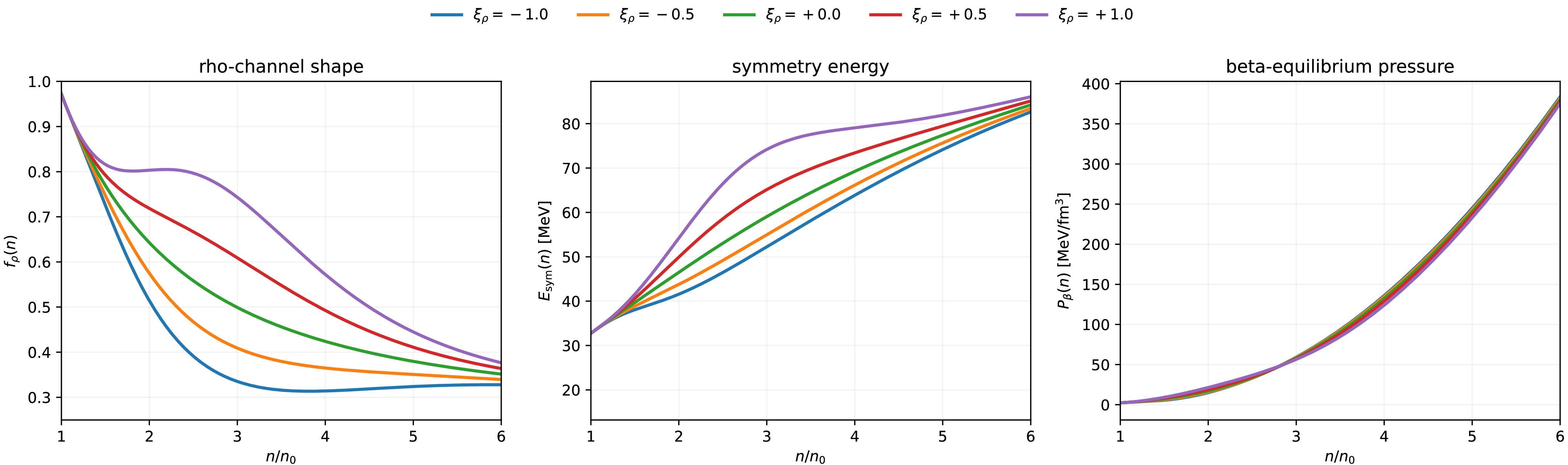
Figure 1. (color online) Density dependence of the ρ-channel shape function
$ f_\rho(n) $ , the symmetry energy$ E_{\rm{sym}}(n) $ , and the beta-equilibrium pressure$ P_\beta(n) $ for representative values of$ \xi_\rho $ .The impact of the same variation on the composition of beta-equilibrated matter is shown in Fig. 2. The proton fraction is obtained from the beta-equilibrium and charge-neutrality conditions,
$ \mu_n-\mu_p=\mu_e=\mu_\mu, n_p=n_e+n_\mu $ . Since the symmetry energy controls the isospin dependence of the energy per baryon, a change in the high-density ρ-channel modifies the high-density proton fraction$ Y_p(n) $ . The direct-Urca process becomes kinematically allowed when the Fermi momenta satisfy the triangle condition [34−36],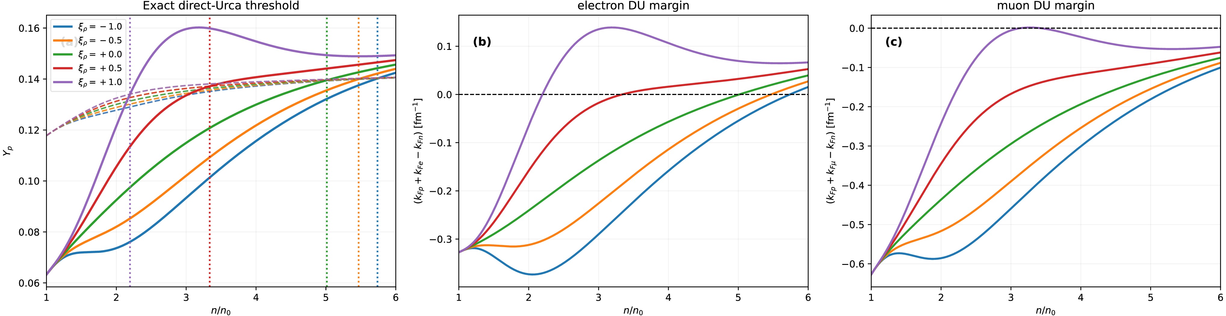
Figure 2. (color online) Direct-Urca threshold diagnostics for representative values of
$ \xi_\rho $ . Panel (a) shows the proton fraction$ Y_p $ and the corresponding direct-Urca threshold in charge-neutral$ npe\mu $ matter. The vertical dotted lines mark the first crossing of the electron direct-Urca threshold. Panels (b) and (c) show the electron and muon direct-Urca margins,$ k_{Fp}+k_{Fe}-k_{Fn} $ and$ k_{Fp}+k_{F\mu}-k_{Fn} $ , respectively. The horizontal dashed lines denote zero margin.$ k_{Fn}\le k_{Fp}+k_{Fl}, \qquad l=e,\mu . $
(36) For the electron channel, this condition can be monitored through the margin
$ \Delta k_e=k_{Fp}+k_{Fe}-k_{Fn} $ , and analogously for the muon channel,$ \Delta k_\mu=k_{Fp}+k_{F\mu}-k_{Fn} $ . The zero crossing of$ \Delta k_l $ defines the onset of the corresponding direct-Urca channel. In the representative cases shown in Fig. 2, the electron channel gives the first onset, while the muon channel appears only after muons are populated and its margin is correspondingly evaluated at higher density.These single-point diagnostics show that
$ \xi_\rho $ primarily changes the high-density isovector and composition-sensitive sector:$ f_\rho(n) \rightarrow E_{\rm{sym}}(n) \rightarrow Y_p(n) \rightarrow n_{\rm{DU}} $ . They also show that the same variation does not act as a leading modification of the bulk beta-equilibrium pressure. This separation motivates the posterior-level comparison below between bulk observables, such as$ P_\beta(n) $ ,$ M - R $ , and$ \Lambda(M) $ , and composition-sensitive observables, such as$ Y_p(n) $ ,$ n_{\rm{DU}} $ , and$ M_{\rm{DU}} $ . -
Before presenting the full Bayesian results, we first illustrate the role of the ρ-flex parameter at the level of a representative EOS. In this diagnostic calculation, the ten baseline parameters are fixed to a representative 10D point, namely
$ \begin{aligned}[b] {\boldsymbol{\theta}}_{10} = \;&\left( K_0, m^*/M, n_0, E_0, E_{\rm{sym}}(n_0), L, K_{\rm{sym}}, f_{\sigma,\infty}, f_{\omega,\infty}, f_{\rho,\infty} \right) \\ &= (242.3\ {\rm{MeV}}, 0.64, 0.15\ {\rm{fm}}^{-3}, -16.1\ {\rm{MeV}},\\& 33.67\ {\rm{MeV}}, 37.29\ {\rm{MeV}}, -87.43\ {\rm{MeV}}, 0.79, 0.78, 0.23 ), \end{aligned} $
(35) while
$ \xi_\rho $ is varied in the range of$ \xi_\rho $ =-1.0, -0.5, 0.0, 0.5, 1.0. This calculation is not used as an additional constraint in the Bayesian inference. Its purpose is to display the channel in which the extra parameter acts and to clarify the quantities that are most directly affected.Figure 1 shows the density dependence of the ρ-channel shape function
$ f_\rho(n) $ , the symmetry energy$ E_{\rm{sym}}(n) $ , and the beta-equilibrium pressure$ P_\beta(n) $ . By construction, all curves coincide at saturation density up to the order fixed by the saturation-point isovector inputs. At suprasaturation densities, varying$ \xi_\rho $ changes the ρ-channel shape and therefore modifies the potential part of the symmetry energy, especially above$ n_0 $ . In contrast, the beta-equilibrium pressure$ P_\beta(n) $ varies more weakly over the same range of$ \xi_\rho $ . This behavior follows from the fact that$ \xi_\rho $ is introduced only in the isovector (ρ) channel, while the isoscalar σ- and ω-channel density dependences are kept fixed.
Figure 1. (color online) Density dependence of the ρ-channel shape function
$ f_\rho(n) $ , the symmetry energy$ E_{\rm{sym}}(n) $ , and the beta-equilibrium pressure$ P_\beta(n) $ for representative values of$ \xi_\rho $ .The impact of the same variation on the composition of beta-equilibrated matter is shown in Fig. 2. The proton fraction is obtained from the beta-equilibrium and charge-neutrality conditions,
$ \mu_n-\mu_p=\mu_e=\mu_\mu, n_p=n_e+n_\mu $ . Since the symmetry energy controls the isospin dependence of the energy per baryon, a change in the high-density ρ-channel modifies the high-density proton fraction$ Y_p(n) $ . The direct-Urca process becomes kinematically allowed when the Fermi momenta satisfy the triangle condition [34−36],
Figure 2. (color online) Direct-Urca threshold diagnostics for representative values of
$ \xi_\rho $ . Panel (a) shows the proton fraction$ Y_p $ and the corresponding direct-Urca threshold in charge-neutral$ npe\mu $ matter. The vertical dotted lines mark the first crossing of the electron direct-Urca threshold. Panels (b) and (c) show the electron and muon direct-Urca margins,$ k_{Fp}+k_{Fe}-k_{Fn} $ and$ k_{Fp}+k_{F\mu}-k_{Fn} $ , respectively. The horizontal dashed lines denote zero margin.$ k_{Fn}\le k_{Fp}+k_{Fl}, \qquad l=e,\mu . $
(36) For the electron channel, this condition can be monitored through the margin
$ \Delta k_e=k_{Fp}+k_{Fe}-k_{Fn} $ , and analogously for the muon channel,$ \Delta k_\mu=k_{Fp}+k_{F\mu}-k_{Fn} $ . The zero crossing of$ \Delta k_l $ defines the onset of the corresponding direct-Urca channel. In the representative cases shown in Fig. 2, the electron channel gives the first onset, while the muon channel appears only after muons are populated and its margin is correspondingly evaluated at higher density.These single-point diagnostics show that
$ \xi_\rho $ primarily changes the high-density isovector and composition-sensitive sector:$ f_\rho(n) \rightarrow E_{\rm{sym}}(n) \rightarrow Y_p(n) \rightarrow n_{\rm{DU}} $ . They also show that the same variation does not act as a leading modification of the bulk beta-equilibrium pressure. This separation motivates the posterior-level comparison below between bulk observables, such as$ P_\beta(n) $ ,$ M - R $ , and$ \Lambda(M) $ , and composition-sensitive observables, such as$ Y_p(n) $ ,$ n_{\rm{DU}} $ , and$ M_{\rm{DU}} $ . -
Before presenting the full Bayesian results, we first illustrate the role of the ρ-flex parameter at the level of a representative EOS. In this diagnostic calculation, the ten baseline parameters are fixed to a representative 10D point, namely
$ \begin{aligned}[b] {\boldsymbol{\theta}}_{10} = \;&\left( K_0, m^*/M, n_0, E_0, E_{\rm{sym}}(n_0), L, K_{\rm{sym}}, f_{\sigma,\infty}, f_{\omega,\infty}, f_{\rho,\infty} \right) \\ &= (242.3\ {\rm{MeV}}, 0.64, 0.15\ {\rm{fm}}^{-3}, -16.1\ {\rm{MeV}},\\& 33.67\ {\rm{MeV}}, 37.29\ {\rm{MeV}}, -87.43\ {\rm{MeV}}, 0.79, 0.78, 0.23 ), \end{aligned} $
(35) while
$ \xi_\rho $ is varied in the range of$ \xi_\rho $ =-1.0, -0.5, 0.0, 0.5, 1.0. This calculation is not used as an additional constraint in the Bayesian inference. Its purpose is to display the channel in which the extra parameter acts and to clarify the quantities that are most directly affected.Figure 1 shows the density dependence of the ρ-channel shape function
$ f_\rho(n) $ , the symmetry energy$ E_{\rm{sym}}(n) $ , and the beta-equilibrium pressure$ P_\beta(n) $ . By construction, all curves coincide at saturation density up to the order fixed by the saturation-point isovector inputs. At suprasaturation densities, varying$ \xi_\rho $ changes the ρ-channel shape and therefore modifies the potential part of the symmetry energy, especially above$ n_0 $ . In contrast, the beta-equilibrium pressure$ P_\beta(n) $ varies more weakly over the same range of$ \xi_\rho $ . This behavior follows from the fact that$ \xi_\rho $ is introduced only in the isovector (ρ) channel, while the isoscalar σ- and ω-channel density dependences are kept fixed.
Figure 1. (color online) Density dependence of the ρ-channel shape function
$ f_\rho(n) $ , the symmetry energy$ E_{\rm{sym}}(n) $ , and the beta-equilibrium pressure$ P_\beta(n) $ for representative values of$ \xi_\rho $ .The impact of the same variation on the composition of beta-equilibrated matter is shown in Fig. 2. The proton fraction is obtained from the beta-equilibrium and charge-neutrality conditions,
$ \mu_n-\mu_p=\mu_e=\mu_\mu, n_p=n_e+n_\mu $ . Since the symmetry energy controls the isospin dependence of the energy per baryon, a change in the high-density ρ-channel modifies the high-density proton fraction$ Y_p(n) $ . The direct-Urca process becomes kinematically allowed when the Fermi momenta satisfy the triangle condition [34−36],
Figure 2. (color online) Direct-Urca threshold diagnostics for representative values of
$ \xi_\rho $ . Panel (a) shows the proton fraction$ Y_p $ and the corresponding direct-Urca threshold in charge-neutral$ npe\mu $ matter. The vertical dotted lines mark the first crossing of the electron direct-Urca threshold. Panels (b) and (c) show the electron and muon direct-Urca margins,$ k_{Fp}+k_{Fe}-k_{Fn} $ and$ k_{Fp}+k_{F\mu}-k_{Fn} $ , respectively. The horizontal dashed lines denote zero margin.$ k_{Fn}\le k_{Fp}+k_{Fl}, \qquad l=e,\mu . $
(36) For the electron channel, this condition can be monitored through the margin
$ \Delta k_e=k_{Fp}+k_{Fe}-k_{Fn} $ , and analogously for the muon channel,$ \Delta k_\mu=k_{Fp}+k_{F\mu}-k_{Fn} $ . The zero crossing of$ \Delta k_l $ defines the onset of the corresponding direct-Urca channel. In the representative cases shown in Fig. 2, the electron channel gives the first onset, while the muon channel appears only after muons are populated and its margin is correspondingly evaluated at higher density.These single-point diagnostics show that
$ \xi_\rho $ primarily changes the high-density isovector and composition-sensitive sector:$ f_\rho(n) \rightarrow E_{\rm{sym}}(n) \rightarrow Y_p(n) \rightarrow n_{\rm{DU}} $ . They also show that the same variation does not act as a leading modification of the bulk beta-equilibrium pressure. This separation motivates the posterior-level comparison below between bulk observables, such as$ P_\beta(n) $ ,$ M - R $ , and$ \Lambda(M) $ , and composition-sensitive observables, such as$ Y_p(n) $ ,$ n_{\rm{DU}} $ , and$ M_{\rm{DU}} $ . -
Before presenting the full Bayesian results, we first illustrate the role of the ρ-flex parameter at the level of a representative EOS. In this diagnostic calculation, the ten baseline parameters are fixed to a representative 10D point, namely
$ \begin{aligned}[b] {\boldsymbol{\theta}}_{10} = \;&\left( K_0, m^*/M, n_0, E_0, E_{\rm{sym}}(n_0), L, K_{\rm{sym}}, f_{\sigma,\infty}, f_{\omega,\infty}, f_{\rho,\infty} \right) \\ &= (242.3\ {\rm{MeV}}, 0.64, 0.15\ {\rm{fm}}^{-3}, -16.1\ {\rm{MeV}},\\& 33.67\ {\rm{MeV}}, 37.29\ {\rm{MeV}}, -87.43\ {\rm{MeV}}, 0.79, 0.78, 0.23 ), \end{aligned} $
(35) while
$ \xi_\rho $ is varied in the range of$ \xi_\rho $ =-1.0, -0.5, 0.0, 0.5, 1.0. This calculation is not used as an additional constraint in the Bayesian inference. Its purpose is to display the channel in which the extra parameter acts and to clarify the quantities that are most directly affected.Figure 1 shows the density dependence of the ρ-channel shape function
$ f_\rho(n) $ , the symmetry energy$ E_{\rm{sym}}(n) $ , and the beta-equilibrium pressure$ P_\beta(n) $ . By construction, all curves coincide at saturation density up to the order fixed by the saturation-point isovector inputs. At suprasaturation densities, varying$ \xi_\rho $ changes the ρ-channel shape and therefore modifies the potential part of the symmetry energy, especially above$ n_0 $ . In contrast, the beta-equilibrium pressure$ P_\beta(n) $ varies more weakly over the same range of$ \xi_\rho $ . This behavior follows from the fact that$ \xi_\rho $ is introduced only in the isovector (ρ) channel, while the isoscalar σ- and ω-channel density dependences are kept fixed.
Figure 1. (color online) Density dependence of the ρ-channel shape function
$ f_\rho(n) $ , the symmetry energy$ E_{\rm{sym}}(n) $ , and the beta-equilibrium pressure$ P_\beta(n) $ for representative values of$ \xi_\rho $ .The impact of the same variation on the composition of beta-equilibrated matter is shown in Fig. 2. The proton fraction is obtained from the beta-equilibrium and charge-neutrality conditions,
$ \mu_n-\mu_p=\mu_e=\mu_\mu, n_p=n_e+n_\mu $ . Since the symmetry energy controls the isospin dependence of the energy per baryon, a change in the high-density ρ-channel modifies the high-density proton fraction$ Y_p(n) $ . The direct-Urca process becomes kinematically allowed when the Fermi momenta satisfy the triangle condition [34−36],
Figure 2. (color online) Direct-Urca threshold diagnostics for representative values of
$ \xi_\rho $ . Panel (a) shows the proton fraction$ Y_p $ and the corresponding direct-Urca threshold in charge-neutral$ npe\mu $ matter. The vertical dotted lines mark the first crossing of the electron direct-Urca threshold. Panels (b) and (c) show the electron and muon direct-Urca margins,$ k_{Fp}+k_{Fe}-k_{Fn} $ and$ k_{Fp}+k_{F\mu}-k_{Fn} $ , respectively. The horizontal dashed lines denote zero margin.$ k_{Fn}\le k_{Fp}+k_{Fl}, \qquad l=e,\mu . $
(36) For the electron channel, this condition can be monitored through the margin
$ \Delta k_e=k_{Fp}+k_{Fe}-k_{Fn} $ , and analogously for the muon channel,$ \Delta k_\mu=k_{Fp}+k_{F\mu}-k_{Fn} $ . The zero crossing of$ \Delta k_l $ defines the onset of the corresponding direct-Urca channel. In the representative cases shown in Fig. 2, the electron channel gives the first onset, while the muon channel appears only after muons are populated and its margin is correspondingly evaluated at higher density.These single-point diagnostics show that
$ \xi_\rho $ primarily changes the high-density isovector and composition-sensitive sector:$ f_\rho(n) \rightarrow E_{\rm{sym}}(n) \rightarrow Y_p(n) \rightarrow n_{\rm{DU}} $ . They also show that the same variation does not act as a leading modification of the bulk beta-equilibrium pressure. This separation motivates the posterior-level comparison below between bulk observables, such as$ P_\beta(n) $ ,$ M - R $ , and$ \Lambda(M) $ , and composition-sensitive observables, such as$ Y_p(n) $ ,$ n_{\rm{DU}} $ , and$ M_{\rm{DU}} $ . -
We first compare the 10D baseline and 11D ρ-flex model at the level of Bayesian evidence. The evidence values are listed in Table 2. For each data set, we define
$ \Delta\ln Z_{\rm{INS}} = \ln Z_{\rm{INS}}^{\rm{11D}} - \ln Z_{\rm{INS}}^{\rm{10D}}, $
(37) where
$ Z_{\rm{INS}} $ denotes the Nested Importance Sampling estimate of the evidence obtained from MultiNest [73]. Positive values of$ \Delta\ln Z_{\rm{INS}} $ favor the 11D ρ-flex model, while negative values favor the 10D baseline. The evidence difference includes the Occam penalty associated with the additional parameter in the 11D model.For the NS+GW data set, we obtain
$ \Delta\ln Z_{\rm{INS}}= -0.23\pm0.08 $ , while for the ALL+GW data set,$ \Delta\ln Z_{\rm{INS}}= -0.02\pm0.17 $ . Both values are close to zero. According to the usual Jeffreys-type interpretation of evidence ratios [74−76], these differences do not constitute decisive support for either model. The present data therefore do not statistically require the additional ρ-channel flexibility parameter. This result is important for the interpretation of the 11D extension. We do not regard$ \xi_\rho $ as an observationally required new degree of freedom. Instead, the 11D model is used as a controlled extension of the 10D baseline to quantify the residual model dependence associated with the assumed high-density continuation of the ρ-channel. The near equality of the evidences indicates that the current data are compatible with both the more restrictive 10D ansatz and the extended 11D ρ-flex parametrization. In the following subsections, we therefore focus not on whether the 11D model improves the global evidence, but on which physical observables are affected when the high-density isovector freedom is relaxed.For completeness, Table 3 lists the posterior summaries of the sampled 11D model parameters for both data sets. The entries are computed from the same posterior samples and with the same mode-plus-90% highest-posterior-density summary routine used for the diagonal annotations in the corresponding corner plots; therefore the table and the corresponding corner-plot diagonals are based on the same values. The table shows that the ALL+GW data set constrains the isoscalar high-density controls
$ f_{\sigma,\infty} $ and$ f_{\omega,\infty} $ , as well as the low-density isovector parameters L and$ K_{\rm{sym}} $ , more strongly than NS+GW. In contrast,$ \xi_\rho $ remains broadly distributed in both data sets, consistent with the evidence result that present data do not require the extra ρ-channel flexibility. As a quantitative prior-dependence diagnostic, we estimated the information gain of$ \xi_\rho $ relative to its uniform prior on$ [-1,1] $ ,Parameter Unit NS+GW ALL+GW $ K_0 $ MeV $ 228.7^{+27.5}_{-6.1} $ $ 233.0^{+23.4}_{-10.6} $ $ m^*/M $ – $ 0.6399^{+0.0100}_{-0.0286} $ $ 0.6437^{+0.0063}_{-0.0208} $ $ n_0 $ fm−3 $ 0.1661^{+0.0039}_{-0.0091} $ $ 0.1475^{+0.0092}_{-0.0024} $ $ E_0 $ MeV $ -16.326^{+0.443}_{-0.142} $ $ -15.979^{+0.137}_{-0.456} $ $ E_{\rm{sym}}(n_0) $ MeV $ 32.45^{+1.83}_{-3.60} $ $ 34.06^{+0.84}_{-3.12} $ L MeV $ 92.9^{+21.5}_{-20.5} $ $ 34.9^{+17.4}_{-8.2} $ $ K_{\rm{sym}} $ MeV $ -268^{+217}_{-128} $ $ -101^{+84}_{-31} $ $ f_{\sigma,\infty} $ – $ 0.743^{+0.112}_{-0.394} $ $ 0.8048^{+0.0306}_{-0.0338} $ $ f_{\omega,\infty} $ – $ 1.228^{+0.166}_{-0.218} $ $ 0.7893^{+0.0287}_{-0.0342} $ $ f_{\rho,\infty} $ – $ 0.555^{+0.230}_{-0.323} $ $ 0.262^{+0.092}_{-0.062} $ $ \xi_\rho $ – $ -0.57^{+1.16}_{-0.41} $ $ -0.54^{+1.04}_{-0.45} $ Table 3. Posterior summaries of the sampled 11D ρ-flex model parameters are listed; each entry gives the posterior mode and the 90% HPD interval for the NS+GW and ALL+GW data sets, computed from the same posterior samples and with the same summary method used for the diagonal annotations in the corresponding corner plots.
$ I_{\xi_\rho} = D_{\rm{KL}} \left[p(\xi_\rho|d)\,\Vert\,p(\xi_\rho)\right]. $
(38) Using the equal-weight posterior chains and a one-dimensional histogram estimate over the prior interval, we obtain
$ I_{\xi_\rho}\simeq0.086 $ nats for NS+GW and$ I_{\xi_\rho}\simeq0.104 $ nats for ALL+GW, corresponding to only about$ 0.12 $ and$ 0.15 $ bits, respectively. The small information gain confirms that the posterior of$ \xi_\rho $ is only weakly compressed relative to the prior. Therefore the broader 11D intervals for high-density isovector and direct-Urca quantities should be interpreted as a conservative estimate of residual model dependence within the adopted ρ-flex prior, rather than as a measurement of a preferred nonzero ρ-channel deformation by the present data. -
We first compare the 10D baseline and 11D ρ-flex model at the level of Bayesian evidence. The evidence values are listed in Table 2. For each data set, we define
$ \Delta\ln Z_{\rm{INS}} = \ln Z_{\rm{INS}}^{\rm{11D}} - \ln Z_{\rm{INS}}^{\rm{10D}}, $
(37) where
$ Z_{\rm{INS}} $ denotes the Nested Importance Sampling estimate of the evidence obtained from MultiNest [73]. Positive values of$ \Delta\ln Z_{\rm{INS}} $ favor the 11D ρ-flex model, while negative values favor the 10D baseline. The evidence difference includes the Occam penalty associated with the additional parameter in the 11D model.For the NS+GW data set, we obtain
$ \Delta\ln Z_{\rm{INS}}= -0.23\pm0.08 $ , while for the ALL+GW data set,$ \Delta\ln Z_{\rm{INS}}= -0.02\pm0.17 $ . Both values are close to zero. According to the usual Jeffreys-type interpretation of evidence ratios [74−76], these differences do not constitute decisive support for either model. The present data therefore do not statistically require the additional ρ-channel flexibility parameter. This result is important for the interpretation of the 11D extension. We do not regard$ \xi_\rho $ as an observationally required new degree of freedom. Instead, the 11D model is used as a controlled extension of the 10D baseline to quantify the residual model dependence associated with the assumed high-density continuation of the ρ-channel. The near equality of the evidences indicates that the current data are compatible with both the more restrictive 10D ansatz and the extended 11D ρ-flex parametrization. In the following subsections, we therefore focus not on whether the 11D model improves the global evidence, but on which physical observables are affected when the high-density isovector freedom is relaxed.For completeness, Table 3 lists the posterior summaries of the sampled 11D model parameters for both data sets. The entries are computed from the same posterior samples and with the same mode-plus-90% highest-posterior-density summary routine used for the diagonal annotations in the corresponding corner plots; therefore the table and the corresponding corner-plot diagonals are based on the same values. The table shows that the ALL+GW data set constrains the isoscalar high-density controls
$ f_{\sigma,\infty} $ and$ f_{\omega,\infty} $ , as well as the low-density isovector parameters L and$ K_{\rm{sym}} $ , more strongly than NS+GW. In contrast,$ \xi_\rho $ remains broadly distributed in both data sets, consistent with the evidence result that present data do not require the extra ρ-channel flexibility. As a quantitative prior-dependence diagnostic, we estimated the information gain of$ \xi_\rho $ relative to its uniform prior on$ [-1,1] $ ,Parameter Unit NS+GW ALL+GW $ K_0 $ MeV $ 228.7^{+27.5}_{-6.1} $ $ 233.0^{+23.4}_{-10.6} $ $ m^*/M $ – $ 0.6399^{+0.0100}_{-0.0286} $ $ 0.6437^{+0.0063}_{-0.0208} $ $ n_0 $ fm−3 $ 0.1661^{+0.0039}_{-0.0091} $ $ 0.1475^{+0.0092}_{-0.0024} $ $ E_0 $ MeV $ -16.326^{+0.443}_{-0.142} $ $ -15.979^{+0.137}_{-0.456} $ $ E_{\rm{sym}}(n_0) $ MeV $ 32.45^{+1.83}_{-3.60} $ $ 34.06^{+0.84}_{-3.12} $ L MeV $ 92.9^{+21.5}_{-20.5} $ $ 34.9^{+17.4}_{-8.2} $ $ K_{\rm{sym}} $ MeV $ -268^{+217}_{-128} $ $ -101^{+84}_{-31} $ $ f_{\sigma,\infty} $ – $ 0.743^{+0.112}_{-0.394} $ $ 0.8048^{+0.0306}_{-0.0338} $ $ f_{\omega,\infty} $ – $ 1.228^{+0.166}_{-0.218} $ $ 0.7893^{+0.0287}_{-0.0342} $ $ f_{\rho,\infty} $ – $ 0.555^{+0.230}_{-0.323} $ $ 0.262^{+0.092}_{-0.062} $ $ \xi_\rho $ – $ -0.57^{+1.16}_{-0.41} $ $ -0.54^{+1.04}_{-0.45} $ Table 3. Posterior summaries of the sampled 11D ρ-flex model parameters are listed; each entry gives the posterior mode and the 90% HPD interval for the NS+GW and ALL+GW data sets, computed from the same posterior samples and with the same summary method used for the diagonal annotations in the corresponding corner plots.
$ I_{\xi_\rho} = D_{\rm{KL}} \left[p(\xi_\rho|d)\,\Vert\,p(\xi_\rho)\right]. $
(38) Using the equal-weight posterior chains and a one-dimensional histogram estimate over the prior interval, we obtain
$ I_{\xi_\rho}\simeq0.086 $ nats for NS+GW and$ I_{\xi_\rho}\simeq0.104 $ nats for ALL+GW, corresponding to only about$ 0.12 $ and$ 0.15 $ bits, respectively. The small information gain confirms that the posterior of$ \xi_\rho $ is only weakly compressed relative to the prior. Therefore the broader 11D intervals for high-density isovector and direct-Urca quantities should be interpreted as a conservative estimate of residual model dependence within the adopted ρ-flex prior, rather than as a measurement of a preferred nonzero ρ-channel deformation by the present data. -
We first compare the 10D baseline and 11D ρ-flex model at the level of Bayesian evidence. The evidence values are listed in Table 2. For each data set, we define
$ \Delta\ln Z_{\rm{INS}} = \ln Z_{\rm{INS}}^{\rm{11D}} - \ln Z_{\rm{INS}}^{\rm{10D}}, $
(37) where
$ Z_{\rm{INS}} $ denotes the Nested Importance Sampling estimate of the evidence obtained from MultiNest [73]. Positive values of$ \Delta\ln Z_{\rm{INS}} $ favor the 11D ρ-flex model, while negative values favor the 10D baseline. The evidence difference includes the Occam penalty associated with the additional parameter in the 11D model.For the NS+GW data set, we obtain
$ \Delta\ln Z_{\rm{INS}}= -0.23\pm0.08 $ , while for the ALL+GW data set,$ \Delta\ln Z_{\rm{INS}}= -0.02\pm0.17 $ . Both values are close to zero. According to the usual Jeffreys-type interpretation of evidence ratios [74−76], these differences do not constitute decisive support for either model. The present data therefore do not statistically require the additional ρ-channel flexibility parameter. This result is important for the interpretation of the 11D extension. We do not regard$ \xi_\rho $ as an observationally required new degree of freedom. Instead, the 11D model is used as a controlled extension of the 10D baseline to quantify the residual model dependence associated with the assumed high-density continuation of the ρ-channel. The near equality of the evidences indicates that the current data are compatible with both the more restrictive 10D ansatz and the extended 11D ρ-flex parametrization. In the following subsections, we therefore focus not on whether the 11D model improves the global evidence, but on which physical observables are affected when the high-density isovector freedom is relaxed.For completeness, Table 3 lists the posterior summaries of the sampled 11D model parameters for both data sets. The entries are computed from the same posterior samples and with the same mode-plus-90% highest-posterior-density summary routine used for the diagonal annotations in the corresponding corner plots; therefore the table and the corresponding corner-plot diagonals are based on the same values. The table shows that the ALL+GW data set constrains the isoscalar high-density controls
$ f_{\sigma,\infty} $ and$ f_{\omega,\infty} $ , as well as the low-density isovector parameters L and$ K_{\rm{sym}} $ , more strongly than NS+GW. In contrast,$ \xi_\rho $ remains broadly distributed in both data sets, consistent with the evidence result that present data do not require the extra ρ-channel flexibility. As a quantitative prior-dependence diagnostic, we estimated the information gain of$ \xi_\rho $ relative to its uniform prior on$ [-1,1] $ ,Parameter Unit NS+GW ALL+GW $ K_0 $ MeV $ 228.7^{+27.5}_{-6.1} $ $ 233.0^{+23.4}_{-10.6} $ $ m^*/M $ – $ 0.6399^{+0.0100}_{-0.0286} $ $ 0.6437^{+0.0063}_{-0.0208} $ $ n_0 $ fm−3 $ 0.1661^{+0.0039}_{-0.0091} $ $ 0.1475^{+0.0092}_{-0.0024} $ $ E_0 $ MeV $ -16.326^{+0.443}_{-0.142} $ $ -15.979^{+0.137}_{-0.456} $ $ E_{\rm{sym}}(n_0) $ MeV $ 32.45^{+1.83}_{-3.60} $ $ 34.06^{+0.84}_{-3.12} $ L MeV $ 92.9^{+21.5}_{-20.5} $ $ 34.9^{+17.4}_{-8.2} $ $ K_{\rm{sym}} $ MeV $ -268^{+217}_{-128} $ $ -101^{+84}_{-31} $ $ f_{\sigma,\infty} $ – $ 0.743^{+0.112}_{-0.394} $ $ 0.8048^{+0.0306}_{-0.0338} $ $ f_{\omega,\infty} $ – $ 1.228^{+0.166}_{-0.218} $ $ 0.7893^{+0.0287}_{-0.0342} $ $ f_{\rho,\infty} $ – $ 0.555^{+0.230}_{-0.323} $ $ 0.262^{+0.092}_{-0.062} $ $ \xi_\rho $ – $ -0.57^{+1.16}_{-0.41} $ $ -0.54^{+1.04}_{-0.45} $ Table 3. Posterior summaries of the sampled 11D ρ-flex model parameters are listed; each entry gives the posterior mode and the 90% HPD interval for the NS+GW and ALL+GW data sets, computed from the same posterior samples and with the same summary method used for the diagonal annotations in the corresponding corner plots.
$ I_{\xi_\rho} = D_{\rm{KL}} \left[p(\xi_\rho|d)\,\Vert\,p(\xi_\rho)\right]. $
(38) Using the equal-weight posterior chains and a one-dimensional histogram estimate over the prior interval, we obtain
$ I_{\xi_\rho}\simeq0.086 $ nats for NS+GW and$ I_{\xi_\rho}\simeq0.104 $ nats for ALL+GW, corresponding to only about$ 0.12 $ and$ 0.15 $ bits, respectively. The small information gain confirms that the posterior of$ \xi_\rho $ is only weakly compressed relative to the prior. Therefore the broader 11D intervals for high-density isovector and direct-Urca quantities should be interpreted as a conservative estimate of residual model dependence within the adopted ρ-flex prior, rather than as a measurement of a preferred nonzero ρ-channel deformation by the present data. -
We first compare the 10D baseline and 11D ρ-flex model at the level of Bayesian evidence. The evidence values are listed in Table 2. For each data set, we define
$ \Delta\ln Z_{\rm{INS}} = \ln Z_{\rm{INS}}^{\rm{11D}} - \ln Z_{\rm{INS}}^{\rm{10D}}, $
(37) where
$ Z_{\rm{INS}} $ denotes the Nested Importance Sampling estimate of the evidence obtained from MultiNest [73]. Positive values of$ \Delta\ln Z_{\rm{INS}} $ favor the 11D ρ-flex model, while negative values favor the 10D baseline. The evidence difference includes the Occam penalty associated with the additional parameter in the 11D model.For the NS+GW data set, we obtain
$ \Delta\ln Z_{\rm{INS}}= -0.23\pm0.08 $ , while for the ALL+GW data set,$ \Delta\ln Z_{\rm{INS}}= -0.02\pm0.17 $ . Both values are close to zero. According to the usual Jeffreys-type interpretation of evidence ratios [74−76], these differences do not constitute decisive support for either model. The present data therefore do not statistically require the additional ρ-channel flexibility parameter. This result is important for the interpretation of the 11D extension. We do not regard$ \xi_\rho $ as an observationally required new degree of freedom. Instead, the 11D model is used as a controlled extension of the 10D baseline to quantify the residual model dependence associated with the assumed high-density continuation of the ρ-channel. The near equality of the evidences indicates that the current data are compatible with both the more restrictive 10D ansatz and the extended 11D ρ-flex parametrization. In the following subsections, we therefore focus not on whether the 11D model improves the global evidence, but on which physical observables are affected when the high-density isovector freedom is relaxed.For completeness, Table 3 lists the posterior summaries of the sampled 11D model parameters for both data sets. The entries are computed from the same posterior samples and with the same mode-plus-90% highest-posterior-density summary routine used for the diagonal annotations in the corresponding corner plots; therefore the table and the corresponding corner-plot diagonals are based on the same values. The table shows that the ALL+GW data set constrains the isoscalar high-density controls
$ f_{\sigma,\infty} $ and$ f_{\omega,\infty} $ , as well as the low-density isovector parameters L and$ K_{\rm{sym}} $ , more strongly than NS+GW. In contrast,$ \xi_\rho $ remains broadly distributed in both data sets, consistent with the evidence result that present data do not require the extra ρ-channel flexibility. As a quantitative prior-dependence diagnostic, we estimated the information gain of$ \xi_\rho $ relative to its uniform prior on$ [-1,1] $ ,Parameter Unit NS+GW ALL+GW $ K_0 $ MeV $ 228.7^{+27.5}_{-6.1} $ $ 233.0^{+23.4}_{-10.6} $ $ m^*/M $ – $ 0.6399^{+0.0100}_{-0.0286} $ $ 0.6437^{+0.0063}_{-0.0208} $ $ n_0 $ fm−3 $ 0.1661^{+0.0039}_{-0.0091} $ $ 0.1475^{+0.0092}_{-0.0024} $ $ E_0 $ MeV $ -16.326^{+0.443}_{-0.142} $ $ -15.979^{+0.137}_{-0.456} $ $ E_{\rm{sym}}(n_0) $ MeV $ 32.45^{+1.83}_{-3.60} $ $ 34.06^{+0.84}_{-3.12} $ L MeV $ 92.9^{+21.5}_{-20.5} $ $ 34.9^{+17.4}_{-8.2} $ $ K_{\rm{sym}} $ MeV $ -268^{+217}_{-128} $ $ -101^{+84}_{-31} $ $ f_{\sigma,\infty} $ – $ 0.743^{+0.112}_{-0.394} $ $ 0.8048^{+0.0306}_{-0.0338} $ $ f_{\omega,\infty} $ – $ 1.228^{+0.166}_{-0.218} $ $ 0.7893^{+0.0287}_{-0.0342} $ $ f_{\rho,\infty} $ – $ 0.555^{+0.230}_{-0.323} $ $ 0.262^{+0.092}_{-0.062} $ $ \xi_\rho $ – $ -0.57^{+1.16}_{-0.41} $ $ -0.54^{+1.04}_{-0.45} $ Table 3. Posterior summaries of the sampled 11D ρ-flex model parameters are listed; each entry gives the posterior mode and the 90% HPD interval for the NS+GW and ALL+GW data sets, computed from the same posterior samples and with the same summary method used for the diagonal annotations in the corresponding corner plots.
$ I_{\xi_\rho} = D_{\rm{KL}} \left[p(\xi_\rho|d)\,\Vert\,p(\xi_\rho)\right]. $
(38) Using the equal-weight posterior chains and a one-dimensional histogram estimate over the prior interval, we obtain
$ I_{\xi_\rho}\simeq0.086 $ nats for NS+GW and$ I_{\xi_\rho}\simeq0.104 $ nats for ALL+GW, corresponding to only about$ 0.12 $ and$ 0.15 $ bits, respectively. The small information gain confirms that the posterior of$ \xi_\rho $ is only weakly compressed relative to the prior. Therefore the broader 11D intervals for high-density isovector and direct-Urca quantities should be interpreted as a conservative estimate of residual model dependence within the adopted ρ-flex prior, rather than as a measurement of a preferred nonzero ρ-channel deformation by the present data. -
We now compare the posterior-predictive results of the 10D baseline and the 11D ρ-flex model. Figure 3 shows the posterior-predictive bands of the symmetry energy
$ E_{\rm{sym}}(n) $ , the proton fraction$ Y_p(n) $ , the mass-radius relation, and the tidal deformability$ \Lambda(M) $ . The upper row corresponds to the NS+GW data set, while the lower row corresponds to ALL+GW. The tidal deformability is obtained consistently from the stellar structure and linear tidal-response equations [77−80]. For both data sets, the 10D and 11D models give similar posterior-predictive mass-radius and tidal-deformability bands. This indicates that the additional ρ-channel flexibility does not lead to a large change in the macroscopic neutron-star observables constrained by the present mass, radius, and gravitational-wave data. In particular, the resulting$ M - R $ and$ \Lambda(M) $ predictions remain close in the two model spaces. This behavior is consistent with the Bayesian evidence comparison in Table 2, which shows no decisive preference for either the 10D or 11D model.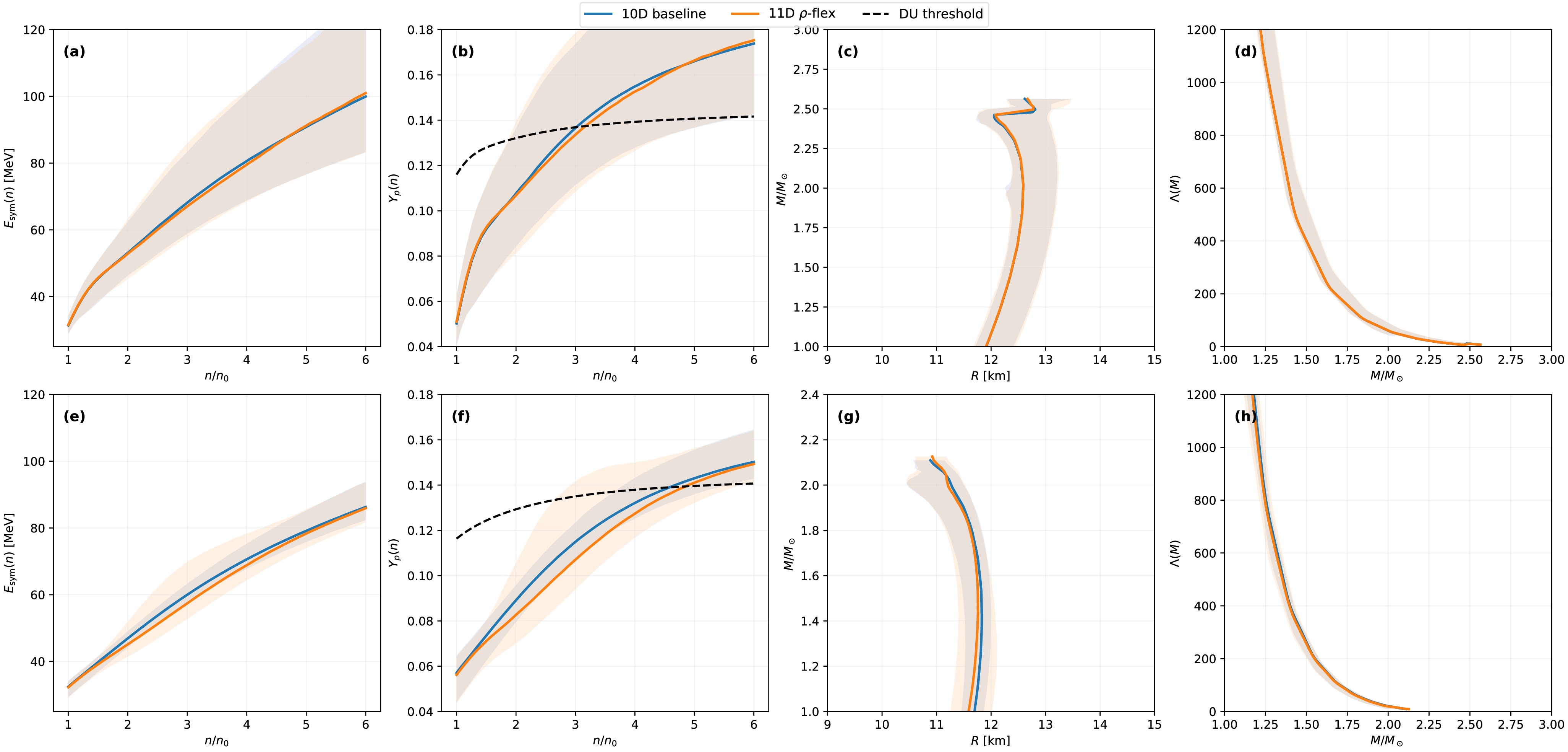
Figure 3. (color online) Posterior predictive comparison between the 10D baseline model and the 11D ρ-flex model. The upper row shows the NS+GW results, while the lower row shows the ALL+GW results. From left to right, the panels display the symmetry energy
$ E_{\rm{sym}}(n) $ , the proton fraction$ Y_p(n) $ in β-equilibrated matter, the mass-radius relation, and the tidal deformability$ \Lambda(M) $ . The solid curves denote representative posterior predictions, and the shaded regions show the corresponding 90% credible bands. Small kinks near the high-mass end of the$ M - R $ bands arise from the termination of different posterior stellar sequences at their own maximum masses and do not indicate a physical discontinuity in the EOS.The differences between the two models are more visible in the isovector and composition sectors. The posterior bands of
$ E_{\rm{sym}}(n) $ and$ Y_p(n) $ show that allowing the extra ρ-channel deformation changes the range of high-density symmetry energy and proton fraction compatible with the adopted constraints. The effect is especially relevant at suprasaturation densities, where the symmetry energy is less directly constrained by terrestrial and astrophysical data [28, 29, 52, 55]. This behavior is expected from the construction of the 11D model, in which$ \xi_\rho $ modifies the high-density ρ-channel while leaving the saturation-point isovector quantities unchanged.To further examine the bulk part of the EOS, Fig. 4 shows the posterior-predictive beta-equilibrium pressure
$ P_\beta(n) $ and squared sound speed$ c_s^2(n) $ . The comparison demonstrates that the 10D and 11D posterior bands of$ P_\beta(n) $ largely overlap in the density region relevant for the stable neutron-star branch. The corresponding sound-speed bands also remain close in the two model spaces. This explains why the macroscopic stellar observables in Fig. 3, especially$ M - R $ and$ \Lambda(M) $ , are only weakly affected by the additional ρ-channel parameter.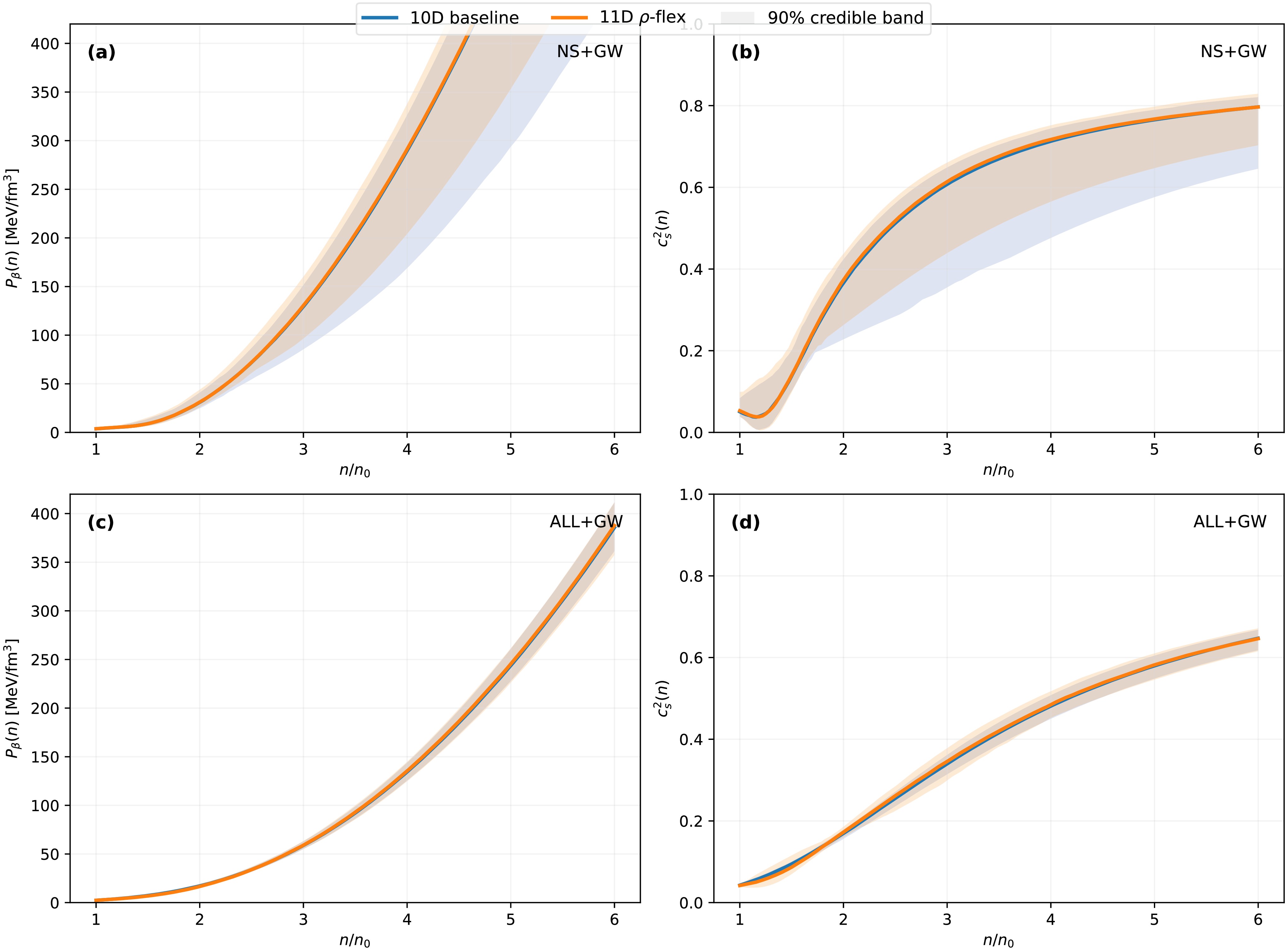
Figure 4. (color online) Posterior-predictive beta-equilibrium pressure
$ P_\beta(n) $ and squared sound speed$ c_s^2(n) $ for the 10D baseline and 11D ρ-flex models. The upper panels correspond to NS+GW, and the lower panels to ALL+GW. The left column shows$ P_\beta(n) $ , and the right column shows$ c_s^2(n) $ . Solid curves denote the posterior representative curves, and shaded regions denote 90% posterior credible bands.The posterior summaries of selected bulk and stellar observables are listed in Table 4. The table includes
$ R_{1.4} $ ,$ R_{2.0} $ ,$ \Lambda_{1.4} $ ,$ \Lambda_{2.0} $ ,$ M_{\max} $ ,$ P_\beta(2n_0) $ ,$ c_s^2[n_c(1.4M_\odot)] $ , and$ c_s^2[n_c(2.0M_\odot)] $ . The tabulated values show the same trend as the posterior-predictive bands: the 10D baseline and the 11D ρ-flex model give comparable bulk pressure, sound speed, radii, tidal deformabilities, and maximum masses for both NS+GW and ALL+GW. Therefore, at the level of bulk stellar structure, the additional parameter$ \xi_\rho $ does not act as a leading stiffness-control parameter. The small bends or apparent abrupt changes near the upper end of the$ M - R $ bands in Fig. 3 should not be interpreted as phase transitions or discontinuities in the EOS. They occur close to the maximum-mass end of the stable branch, where different posterior samples terminate at different$ M_{\max} $ values and the credible band is constructed from a rapidly changing subset of stellar sequences. Thus the high-mass edge of the plotted band is more sensitive to finite posterior sampling and interpolation than the well-populated mass range below about$ 2M_\odot $ .Data set Model $ R_{1.4} $ km$ R_{2.0} $ km$ \Lambda_{1.4} $ $ \Lambda_{2.0} $ $ M_{\max} $ $ M_\odot $ $ P_\beta(2n_0) $ MeV fm-3$ c_s^2[n_c(1.4M_\odot)] $ $ c_s^2[n_c(2.0M_\odot)] $ NS+GW 10D $ 12.28^{+0.56}_{-0.14} $ $ 12.57^{+0.66}_{-0.16} $ $ 565^{+199}_{-53} $ $ 59.5^{+32.0}_{-5.6} $ $ 2.455^{+0.152}_{-0.044} $ $ 31.6^{+7.2}_{-7.0} $ $ 0.455^{+0.027}_{-0.039} $ $ 0.596^{+0.017}_{-0.028} $ NS+GW 11D $ 12.27^{+0.58}_{-0.15} $ $ 12.57^{+0.69}_{-0.15} $ $ 560^{+216}_{-55} $ $ 59.8^{+33.1}_{-5.7} $ $ 2.462^{+0.158}_{-0.069} $ $ 31.7^{+8.2}_{-8.4} $ $ 0.463^{+0.032}_{-0.067} $ $ 0.604^{+0.019}_{-0.057} $ ALL+GW 10D $ 11.88^{+0.13}_{-0.33} $ $ 11.35^{+0.18}_{-0.83} $ $ 409^{+54}_{-65} $ $ 21.6^{+3.9}_{-11.3} $ $ 2.102^{+0.028}_{-0.092} $ $ 17.0^{+1.5}_{-1.1} $ $ 0.374^{+0.012}_{-0.018} $ $ 0.603^{+0.059}_{-0.014} $ ALL+GW 11D $ 11.80^{+0.20}_{-0.43} $ $ 11.38^{+0.21}_{-0.77} $ $ 398^{+59}_{-88} $ $ 23.0^{+3.3}_{-12.2} $ $ 2.111^{+0.026}_{-0.105} $ $ 15.8^{+3.6}_{-1.3} $ $ 0.383^{+0.018}_{-0.040} $ $ 0.594^{+0.063}_{-0.014} $ Table 4. Posterior summaries of bulk and macroscopic neutron-star observables for the 10D baseline and 11D ρ-flex models. Entries report the posterior mode and the 90% HPD interval.
This separation between bulk and isovector responses is central to the interpretation of the ρ-flex extension. The present constraints determine the beta-equilibrated bulk EOS sufficiently well that the additional high-density ρ-channel freedom has only a limited impact on
$ M - R $ ,$ \Lambda(M) $ , and$ M_{\max} $ . At the same time, the high-density composition, through$ E_{\rm{sym}}(n) $ and$ Y_p(n) $ , remains sensitive to the ρ-channel ansatz. The consequences of this residual isovector uncertainty for the direct-Urca threshold are examined in the next subsection.The systematic reduction of
$ M_{\max} $ from NS+GW to ALL+GW in Table 4 is a consequence of the additional pressure-band constraints rather than of the ρ-flex extension itself. It appears in both the 10D and 11D analyses. The HIC likelihood is the main additional constraint on the high-density stiffness because it acts directly on the symmetric-nuclear-matter pressure over the suprasaturation-density range$ u=n/n_0=1.3 $ −4.5. It removes the very stiff high-density isoscalar-vector sector allowed by NS+GW alone; for example, in the 11D posterior the mode of$ f_{\omega,\infty} $ shifts from 1.228 for NS+GW to 0.789 for ALL+GW. The χEFT band mainly constrains the low-density neutron-rich EOS and, together with the HIC pressure band, lowers the beta-equilibrium pressure around$ 2n_0 $ , from about$ 32 $ to$ 16 $ –$ 17 $ MeV fm-3. The resulting ALL+GW posterior therefore favors a softer EOS whose maximum mass lies close to the imposed massive-pulsar lower-bound likelihood, while still satisfying the$ 2M_\odot $ constraint. Thus the lower$ M_{\max} $ in ALL+GW reflects the adopted χEFT+HIC pressure likelihoods, with the high-density HIC term providing the dominant stiffness constraint. -
We now compare the posterior-predictive results of the 10D baseline and the 11D ρ-flex model. Figure 3 shows the posterior-predictive bands of the symmetry energy
$ E_{\rm{sym}}(n) $ , the proton fraction$ Y_p(n) $ , the mass-radius relation, and the tidal deformability$ \Lambda(M) $ . The upper row corresponds to the NS+GW data set, while the lower row corresponds to ALL+GW. The tidal deformability is obtained consistently from the stellar structure and linear tidal-response equations [77−80]. For both data sets, the 10D and 11D models give similar posterior-predictive mass-radius and tidal-deformability bands. This indicates that the additional ρ-channel flexibility does not lead to a large change in the macroscopic neutron-star observables constrained by the present mass, radius, and gravitational-wave data. In particular, the resulting$ M - R $ and$ \Lambda(M) $ predictions remain close in the two model spaces. This behavior is consistent with the Bayesian evidence comparison in Table 2, which shows no decisive preference for either the 10D or 11D model.
Figure 3. (color online) Posterior predictive comparison between the 10D baseline model and the 11D ρ-flex model. The upper row shows the NS+GW results, while the lower row shows the ALL+GW results. From left to right, the panels display the symmetry energy
$ E_{\rm{sym}}(n) $ , the proton fraction$ Y_p(n) $ in β-equilibrated matter, the mass-radius relation, and the tidal deformability$ \Lambda(M) $ . The solid curves denote representative posterior predictions, and the shaded regions show the corresponding 90% credible bands. Small kinks near the high-mass end of the$ M - R $ bands arise from the termination of different posterior stellar sequences at their own maximum masses and do not indicate a physical discontinuity in the EOS.The differences between the two models are more visible in the isovector and composition sectors. The posterior bands of
$ E_{\rm{sym}}(n) $ and$ Y_p(n) $ show that allowing the extra ρ-channel deformation changes the range of high-density symmetry energy and proton fraction compatible with the adopted constraints. The effect is especially relevant at suprasaturation densities, where the symmetry energy is less directly constrained by terrestrial and astrophysical data [28, 29, 52, 55]. This behavior is expected from the construction of the 11D model, in which$ \xi_\rho $ modifies the high-density ρ-channel while leaving the saturation-point isovector quantities unchanged.To further examine the bulk part of the EOS, Fig. 4 shows the posterior-predictive beta-equilibrium pressure
$ P_\beta(n) $ and squared sound speed$ c_s^2(n) $ . The comparison demonstrates that the 10D and 11D posterior bands of$ P_\beta(n) $ largely overlap in the density region relevant for the stable neutron-star branch. The corresponding sound-speed bands also remain close in the two model spaces. This explains why the macroscopic stellar observables in Fig. 3, especially$ M - R $ and$ \Lambda(M) $ , are only weakly affected by the additional ρ-channel parameter.
Figure 4. (color online) Posterior-predictive beta-equilibrium pressure
$ P_\beta(n) $ and squared sound speed$ c_s^2(n) $ for the 10D baseline and 11D ρ-flex models. The upper panels correspond to NS+GW, and the lower panels to ALL+GW. The left column shows$ P_\beta(n) $ , and the right column shows$ c_s^2(n) $ . Solid curves denote the posterior representative curves, and shaded regions denote 90% posterior credible bands.The posterior summaries of selected bulk and stellar observables are listed in Table 4. The table includes
$ R_{1.4} $ ,$ R_{2.0} $ ,$ \Lambda_{1.4} $ ,$ \Lambda_{2.0} $ ,$ M_{\max} $ ,$ P_\beta(2n_0) $ ,$ c_s^2[n_c(1.4M_\odot)] $ , and$ c_s^2[n_c(2.0M_\odot)] $ . The tabulated values show the same trend as the posterior-predictive bands: the 10D baseline and the 11D ρ-flex model give comparable bulk pressure, sound speed, radii, tidal deformabilities, and maximum masses for both NS+GW and ALL+GW. Therefore, at the level of bulk stellar structure, the additional parameter$ \xi_\rho $ does not act as a leading stiffness-control parameter. The small bends or apparent abrupt changes near the upper end of the$ M - R $ bands in Fig. 3 should not be interpreted as phase transitions or discontinuities in the EOS. They occur close to the maximum-mass end of the stable branch, where different posterior samples terminate at different$ M_{\max} $ values and the credible band is constructed from a rapidly changing subset of stellar sequences. Thus the high-mass edge of the plotted band is more sensitive to finite posterior sampling and interpolation than the well-populated mass range below about$ 2M_\odot $ .Data set Model $ R_{1.4} $ km$ R_{2.0} $ km$ \Lambda_{1.4} $ $ \Lambda_{2.0} $ $ M_{\max} $ $ M_\odot $ $ P_\beta(2n_0) $ MeV fm-3$ c_s^2[n_c(1.4M_\odot)] $ $ c_s^2[n_c(2.0M_\odot)] $ NS+GW 10D $ 12.28^{+0.56}_{-0.14} $ $ 12.57^{+0.66}_{-0.16} $ $ 565^{+199}_{-53} $ $ 59.5^{+32.0}_{-5.6} $ $ 2.455^{+0.152}_{-0.044} $ $ 31.6^{+7.2}_{-7.0} $ $ 0.455^{+0.027}_{-0.039} $ $ 0.596^{+0.017}_{-0.028} $ NS+GW 11D $ 12.27^{+0.58}_{-0.15} $ $ 12.57^{+0.69}_{-0.15} $ $ 560^{+216}_{-55} $ $ 59.8^{+33.1}_{-5.7} $ $ 2.462^{+0.158}_{-0.069} $ $ 31.7^{+8.2}_{-8.4} $ $ 0.463^{+0.032}_{-0.067} $ $ 0.604^{+0.019}_{-0.057} $ ALL+GW 10D $ 11.88^{+0.13}_{-0.33} $ $ 11.35^{+0.18}_{-0.83} $ $ 409^{+54}_{-65} $ $ 21.6^{+3.9}_{-11.3} $ $ 2.102^{+0.028}_{-0.092} $ $ 17.0^{+1.5}_{-1.1} $ $ 0.374^{+0.012}_{-0.018} $ $ 0.603^{+0.059}_{-0.014} $ ALL+GW 11D $ 11.80^{+0.20}_{-0.43} $ $ 11.38^{+0.21}_{-0.77} $ $ 398^{+59}_{-88} $ $ 23.0^{+3.3}_{-12.2} $ $ 2.111^{+0.026}_{-0.105} $ $ 15.8^{+3.6}_{-1.3} $ $ 0.383^{+0.018}_{-0.040} $ $ 0.594^{+0.063}_{-0.014} $ Table 4. Posterior summaries of bulk and macroscopic neutron-star observables for the 10D baseline and 11D ρ-flex models. Entries report the posterior mode and the 90% HPD interval.
This separation between bulk and isovector responses is central to the interpretation of the ρ-flex extension. The present constraints determine the beta-equilibrated bulk EOS sufficiently well that the additional high-density ρ-channel freedom has only a limited impact on
$ M - R $ ,$ \Lambda(M) $ , and$ M_{\max} $ . At the same time, the high-density composition, through$ E_{\rm{sym}}(n) $ and$ Y_p(n) $ , remains sensitive to the ρ-channel ansatz. The consequences of this residual isovector uncertainty for the direct-Urca threshold are examined in the next subsection.The systematic reduction of
$ M_{\max} $ from NS+GW to ALL+GW in Table 4 is a consequence of the additional pressure-band constraints rather than of the ρ-flex extension itself. It appears in both the 10D and 11D analyses. The HIC likelihood is the main additional constraint on the high-density stiffness because it acts directly on the symmetric-nuclear-matter pressure over the suprasaturation-density range$ u=n/n_0=1.3 $ −4.5. It removes the very stiff high-density isoscalar-vector sector allowed by NS+GW alone; for example, in the 11D posterior the mode of$ f_{\omega,\infty} $ shifts from 1.228 for NS+GW to 0.789 for ALL+GW. The χEFT band mainly constrains the low-density neutron-rich EOS and, together with the HIC pressure band, lowers the beta-equilibrium pressure around$ 2n_0 $ , from about$ 32 $ to$ 16 $ –$ 17 $ MeV fm-3. The resulting ALL+GW posterior therefore favors a softer EOS whose maximum mass lies close to the imposed massive-pulsar lower-bound likelihood, while still satisfying the$ 2M_\odot $ constraint. Thus the lower$ M_{\max} $ in ALL+GW reflects the adopted χEFT+HIC pressure likelihoods, with the high-density HIC term providing the dominant stiffness constraint. -
We now compare the posterior-predictive results of the 10D baseline and the 11D ρ-flex model. Figure 3 shows the posterior-predictive bands of the symmetry energy
$ E_{\rm{sym}}(n) $ , the proton fraction$ Y_p(n) $ , the mass-radius relation, and the tidal deformability$ \Lambda(M) $ . The upper row corresponds to the NS+GW data set, while the lower row corresponds to ALL+GW. The tidal deformability is obtained consistently from the stellar structure and linear tidal-response equations [77−80]. For both data sets, the 10D and 11D models give similar posterior-predictive mass-radius and tidal-deformability bands. This indicates that the additional ρ-channel flexibility does not lead to a large change in the macroscopic neutron-star observables constrained by the present mass, radius, and gravitational-wave data. In particular, the resulting$ M - R $ and$ \Lambda(M) $ predictions remain close in the two model spaces. This behavior is consistent with the Bayesian evidence comparison in Table 2, which shows no decisive preference for either the 10D or 11D model.
Figure 3. (color online) Posterior predictive comparison between the 10D baseline model and the 11D ρ-flex model. The upper row shows the NS+GW results, while the lower row shows the ALL+GW results. From left to right, the panels display the symmetry energy
$ E_{\rm{sym}}(n) $ , the proton fraction$ Y_p(n) $ in β-equilibrated matter, the mass-radius relation, and the tidal deformability$ \Lambda(M) $ . The solid curves denote representative posterior predictions, and the shaded regions show the corresponding 90% credible bands. Small kinks near the high-mass end of the$ M - R $ bands arise from the termination of different posterior stellar sequences at their own maximum masses and do not indicate a physical discontinuity in the EOS.The differences between the two models are more visible in the isovector and composition sectors. The posterior bands of
$ E_{\rm{sym}}(n) $ and$ Y_p(n) $ show that allowing the extra ρ-channel deformation changes the range of high-density symmetry energy and proton fraction compatible with the adopted constraints. The effect is especially relevant at suprasaturation densities, where the symmetry energy is less directly constrained by terrestrial and astrophysical data [28, 29, 52, 55]. This behavior is expected from the construction of the 11D model, in which$ \xi_\rho $ modifies the high-density ρ-channel while leaving the saturation-point isovector quantities unchanged.To further examine the bulk part of the EOS, Fig. 4 shows the posterior-predictive beta-equilibrium pressure
$ P_\beta(n) $ and squared sound speed$ c_s^2(n) $ . The comparison demonstrates that the 10D and 11D posterior bands of$ P_\beta(n) $ largely overlap in the density region relevant for the stable neutron-star branch. The corresponding sound-speed bands also remain close in the two model spaces. This explains why the macroscopic stellar observables in Fig. 3, especially$ M - R $ and$ \Lambda(M) $ , are only weakly affected by the additional ρ-channel parameter.
Figure 4. (color online) Posterior-predictive beta-equilibrium pressure
$ P_\beta(n) $ and squared sound speed$ c_s^2(n) $ for the 10D baseline and 11D ρ-flex models. The upper panels correspond to NS+GW, and the lower panels to ALL+GW. The left column shows$ P_\beta(n) $ , and the right column shows$ c_s^2(n) $ . Solid curves denote the posterior representative curves, and shaded regions denote 90% posterior credible bands.The posterior summaries of selected bulk and stellar observables are listed in Table 4. The table includes
$ R_{1.4} $ ,$ R_{2.0} $ ,$ \Lambda_{1.4} $ ,$ \Lambda_{2.0} $ ,$ M_{\max} $ ,$ P_\beta(2n_0) $ ,$ c_s^2[n_c(1.4M_\odot)] $ , and$ c_s^2[n_c(2.0M_\odot)] $ . The tabulated values show the same trend as the posterior-predictive bands: the 10D baseline and the 11D ρ-flex model give comparable bulk pressure, sound speed, radii, tidal deformabilities, and maximum masses for both NS+GW and ALL+GW. Therefore, at the level of bulk stellar structure, the additional parameter$ \xi_\rho $ does not act as a leading stiffness-control parameter. The small bends or apparent abrupt changes near the upper end of the$ M - R $ bands in Fig. 3 should not be interpreted as phase transitions or discontinuities in the EOS. They occur close to the maximum-mass end of the stable branch, where different posterior samples terminate at different$ M_{\max} $ values and the credible band is constructed from a rapidly changing subset of stellar sequences. Thus the high-mass edge of the plotted band is more sensitive to finite posterior sampling and interpolation than the well-populated mass range below about$ 2M_\odot $ .Data set Model $ R_{1.4} $ km$ R_{2.0} $ km$ \Lambda_{1.4} $ $ \Lambda_{2.0} $ $ M_{\max} $ $ M_\odot $ $ P_\beta(2n_0) $ MeV fm-3$ c_s^2[n_c(1.4M_\odot)] $ $ c_s^2[n_c(2.0M_\odot)] $ NS+GW 10D $ 12.28^{+0.56}_{-0.14} $ $ 12.57^{+0.66}_{-0.16} $ $ 565^{+199}_{-53} $ $ 59.5^{+32.0}_{-5.6} $ $ 2.455^{+0.152}_{-0.044} $ $ 31.6^{+7.2}_{-7.0} $ $ 0.455^{+0.027}_{-0.039} $ $ 0.596^{+0.017}_{-0.028} $ NS+GW 11D $ 12.27^{+0.58}_{-0.15} $ $ 12.57^{+0.69}_{-0.15} $ $ 560^{+216}_{-55} $ $ 59.8^{+33.1}_{-5.7} $ $ 2.462^{+0.158}_{-0.069} $ $ 31.7^{+8.2}_{-8.4} $ $ 0.463^{+0.032}_{-0.067} $ $ 0.604^{+0.019}_{-0.057} $ ALL+GW 10D $ 11.88^{+0.13}_{-0.33} $ $ 11.35^{+0.18}_{-0.83} $ $ 409^{+54}_{-65} $ $ 21.6^{+3.9}_{-11.3} $ $ 2.102^{+0.028}_{-0.092} $ $ 17.0^{+1.5}_{-1.1} $ $ 0.374^{+0.012}_{-0.018} $ $ 0.603^{+0.059}_{-0.014} $ ALL+GW 11D $ 11.80^{+0.20}_{-0.43} $ $ 11.38^{+0.21}_{-0.77} $ $ 398^{+59}_{-88} $ $ 23.0^{+3.3}_{-12.2} $ $ 2.111^{+0.026}_{-0.105} $ $ 15.8^{+3.6}_{-1.3} $ $ 0.383^{+0.018}_{-0.040} $ $ 0.594^{+0.063}_{-0.014} $ Table 4. Posterior summaries of bulk and macroscopic neutron-star observables for the 10D baseline and 11D ρ-flex models. Entries report the posterior mode and the 90% HPD interval.
This separation between bulk and isovector responses is central to the interpretation of the ρ-flex extension. The present constraints determine the beta-equilibrated bulk EOS sufficiently well that the additional high-density ρ-channel freedom has only a limited impact on
$ M - R $ ,$ \Lambda(M) $ , and$ M_{\max} $ . At the same time, the high-density composition, through$ E_{\rm{sym}}(n) $ and$ Y_p(n) $ , remains sensitive to the ρ-channel ansatz. The consequences of this residual isovector uncertainty for the direct-Urca threshold are examined in the next subsection.The systematic reduction of
$ M_{\max} $ from NS+GW to ALL+GW in Table 4 is a consequence of the additional pressure-band constraints rather than of the ρ-flex extension itself. It appears in both the 10D and 11D analyses. The HIC likelihood is the main additional constraint on the high-density stiffness because it acts directly on the symmetric-nuclear-matter pressure over the suprasaturation-density range$ u=n/n_0=1.3 $ −4.5. It removes the very stiff high-density isoscalar-vector sector allowed by NS+GW alone; for example, in the 11D posterior the mode of$ f_{\omega,\infty} $ shifts from 1.228 for NS+GW to 0.789 for ALL+GW. The χEFT band mainly constrains the low-density neutron-rich EOS and, together with the HIC pressure band, lowers the beta-equilibrium pressure around$ 2n_0 $ , from about$ 32 $ to$ 16 $ –$ 17 $ MeV fm-3. The resulting ALL+GW posterior therefore favors a softer EOS whose maximum mass lies close to the imposed massive-pulsar lower-bound likelihood, while still satisfying the$ 2M_\odot $ constraint. Thus the lower$ M_{\max} $ in ALL+GW reflects the adopted χEFT+HIC pressure likelihoods, with the high-density HIC term providing the dominant stiffness constraint. -
We now compare the posterior-predictive results of the 10D baseline and the 11D ρ-flex model. Figure 3 shows the posterior-predictive bands of the symmetry energy
$ E_{\rm{sym}}(n) $ , the proton fraction$ Y_p(n) $ , the mass-radius relation, and the tidal deformability$ \Lambda(M) $ . The upper row corresponds to the NS+GW data set, while the lower row corresponds to ALL+GW. The tidal deformability is obtained consistently from the stellar structure and linear tidal-response equations [77−80]. For both data sets, the 10D and 11D models give similar posterior-predictive mass-radius and tidal-deformability bands. This indicates that the additional ρ-channel flexibility does not lead to a large change in the macroscopic neutron-star observables constrained by the present mass, radius, and gravitational-wave data. In particular, the resulting$ M - R $ and$ \Lambda(M) $ predictions remain close in the two model spaces. This behavior is consistent with the Bayesian evidence comparison in Table 2, which shows no decisive preference for either the 10D or 11D model.
Figure 3. (color online) Posterior predictive comparison between the 10D baseline model and the 11D ρ-flex model. The upper row shows the NS+GW results, while the lower row shows the ALL+GW results. From left to right, the panels display the symmetry energy
$ E_{\rm{sym}}(n) $ , the proton fraction$ Y_p(n) $ in β-equilibrated matter, the mass-radius relation, and the tidal deformability$ \Lambda(M) $ . The solid curves denote representative posterior predictions, and the shaded regions show the corresponding 90% credible bands. Small kinks near the high-mass end of the$ M - R $ bands arise from the termination of different posterior stellar sequences at their own maximum masses and do not indicate a physical discontinuity in the EOS.The differences between the two models are more visible in the isovector and composition sectors. The posterior bands of
$ E_{\rm{sym}}(n) $ and$ Y_p(n) $ show that allowing the extra ρ-channel deformation changes the range of high-density symmetry energy and proton fraction compatible with the adopted constraints. The effect is especially relevant at suprasaturation densities, where the symmetry energy is less directly constrained by terrestrial and astrophysical data [28, 29, 52, 55]. This behavior is expected from the construction of the 11D model, in which$ \xi_\rho $ modifies the high-density ρ-channel while leaving the saturation-point isovector quantities unchanged.To further examine the bulk part of the EOS, Fig. 4 shows the posterior-predictive beta-equilibrium pressure
$ P_\beta(n) $ and squared sound speed$ c_s^2(n) $ . The comparison demonstrates that the 10D and 11D posterior bands of$ P_\beta(n) $ largely overlap in the density region relevant for the stable neutron-star branch. The corresponding sound-speed bands also remain close in the two model spaces. This explains why the macroscopic stellar observables in Fig. 3, especially$ M - R $ and$ \Lambda(M) $ , are only weakly affected by the additional ρ-channel parameter.
Figure 4. (color online) Posterior-predictive beta-equilibrium pressure
$ P_\beta(n) $ and squared sound speed$ c_s^2(n) $ for the 10D baseline and 11D ρ-flex models. The upper panels correspond to NS+GW, and the lower panels to ALL+GW. The left column shows$ P_\beta(n) $ , and the right column shows$ c_s^2(n) $ . Solid curves denote the posterior representative curves, and shaded regions denote 90% posterior credible bands.The posterior summaries of selected bulk and stellar observables are listed in Table 4. The table includes
$ R_{1.4} $ ,$ R_{2.0} $ ,$ \Lambda_{1.4} $ ,$ \Lambda_{2.0} $ ,$ M_{\max} $ ,$ P_\beta(2n_0) $ ,$ c_s^2[n_c(1.4M_\odot)] $ , and$ c_s^2[n_c(2.0M_\odot)] $ . The tabulated values show the same trend as the posterior-predictive bands: the 10D baseline and the 11D ρ-flex model give comparable bulk pressure, sound speed, radii, tidal deformabilities, and maximum masses for both NS+GW and ALL+GW. Therefore, at the level of bulk stellar structure, the additional parameter$ \xi_\rho $ does not act as a leading stiffness-control parameter. The small bends or apparent abrupt changes near the upper end of the$ M - R $ bands in Fig. 3 should not be interpreted as phase transitions or discontinuities in the EOS. They occur close to the maximum-mass end of the stable branch, where different posterior samples terminate at different$ M_{\max} $ values and the credible band is constructed from a rapidly changing subset of stellar sequences. Thus the high-mass edge of the plotted band is more sensitive to finite posterior sampling and interpolation than the well-populated mass range below about$ 2M_\odot $ .Data set Model $ R_{1.4} $ km$ R_{2.0} $ km$ \Lambda_{1.4} $ $ \Lambda_{2.0} $ $ M_{\max} $ $ M_\odot $ $ P_\beta(2n_0) $ MeV fm-3$ c_s^2[n_c(1.4M_\odot)] $ $ c_s^2[n_c(2.0M_\odot)] $ NS+GW 10D $ 12.28^{+0.56}_{-0.14} $ $ 12.57^{+0.66}_{-0.16} $ $ 565^{+199}_{-53} $ $ 59.5^{+32.0}_{-5.6} $ $ 2.455^{+0.152}_{-0.044} $ $ 31.6^{+7.2}_{-7.0} $ $ 0.455^{+0.027}_{-0.039} $ $ 0.596^{+0.017}_{-0.028} $ NS+GW 11D $ 12.27^{+0.58}_{-0.15} $ $ 12.57^{+0.69}_{-0.15} $ $ 560^{+216}_{-55} $ $ 59.8^{+33.1}_{-5.7} $ $ 2.462^{+0.158}_{-0.069} $ $ 31.7^{+8.2}_{-8.4} $ $ 0.463^{+0.032}_{-0.067} $ $ 0.604^{+0.019}_{-0.057} $ ALL+GW 10D $ 11.88^{+0.13}_{-0.33} $ $ 11.35^{+0.18}_{-0.83} $ $ 409^{+54}_{-65} $ $ 21.6^{+3.9}_{-11.3} $ $ 2.102^{+0.028}_{-0.092} $ $ 17.0^{+1.5}_{-1.1} $ $ 0.374^{+0.012}_{-0.018} $ $ 0.603^{+0.059}_{-0.014} $ ALL+GW 11D $ 11.80^{+0.20}_{-0.43} $ $ 11.38^{+0.21}_{-0.77} $ $ 398^{+59}_{-88} $ $ 23.0^{+3.3}_{-12.2} $ $ 2.111^{+0.026}_{-0.105} $ $ 15.8^{+3.6}_{-1.3} $ $ 0.383^{+0.018}_{-0.040} $ $ 0.594^{+0.063}_{-0.014} $ Table 4. Posterior summaries of bulk and macroscopic neutron-star observables for the 10D baseline and 11D ρ-flex models. Entries report the posterior mode and the 90% HPD interval.
This separation between bulk and isovector responses is central to the interpretation of the ρ-flex extension. The present constraints determine the beta-equilibrated bulk EOS sufficiently well that the additional high-density ρ-channel freedom has only a limited impact on
$ M - R $ ,$ \Lambda(M) $ , and$ M_{\max} $ . At the same time, the high-density composition, through$ E_{\rm{sym}}(n) $ and$ Y_p(n) $ , remains sensitive to the ρ-channel ansatz. The consequences of this residual isovector uncertainty for the direct-Urca threshold are examined in the next subsection.The systematic reduction of
$ M_{\max} $ from NS+GW to ALL+GW in Table 4 is a consequence of the additional pressure-band constraints rather than of the ρ-flex extension itself. It appears in both the 10D and 11D analyses. The HIC likelihood is the main additional constraint on the high-density stiffness because it acts directly on the symmetric-nuclear-matter pressure over the suprasaturation-density range$ u=n/n_0=1.3 $ −4.5. It removes the very stiff high-density isoscalar-vector sector allowed by NS+GW alone; for example, in the 11D posterior the mode of$ f_{\omega,\infty} $ shifts from 1.228 for NS+GW to 0.789 for ALL+GW. The χEFT band mainly constrains the low-density neutron-rich EOS and, together with the HIC pressure band, lowers the beta-equilibrium pressure around$ 2n_0 $ , from about$ 32 $ to$ 16 $ –$ 17 $ MeV fm-3. The resulting ALL+GW posterior therefore favors a softer EOS whose maximum mass lies close to the imposed massive-pulsar lower-bound likelihood, while still satisfying the$ 2M_\odot $ constraint. Thus the lower$ M_{\max} $ in ALL+GW reflects the adopted χEFT+HIC pressure likelihoods, with the high-density HIC term providing the dominant stiffness constraint. -
We next examine how the high-density isovector uncertainty affects the direct-Urca threshold. The nucleonic direct-Urca process,
$ n\rightarrow p+l+\bar{\nu}_l, \qquad p+l\rightarrow n+\nu_l, \qquad l=e,\mu , $
(39) is kinematically allowed when the Fermi momenta satisfy the triangle condition in Eq. (36). For a given EOS, this condition defines the direct-Urca threshold density
$ n_{\rm{DU}} $ . If the central density of a star of mass M, denoted$ n_c(M) $ , exceeds this threshold, the direct-Urca channel is open in the stellar core.Figure 5 compares the posterior central-density curves
$ n_c(M) $ with the corresponding direct-Urca threshold density$ n_{\rm{DU}} $ . The results are shown separately for NS+GW and ALL+GW. For each model, the stellar sequence determines$ n_c(M) $ , while the composition of beta-equilibrated matter determines$ n_{\rm{DU}} $ . Thus, the onset of direct Urca in a star of mass M depends on the relative position of these two quantities. The 10D and 11D models can have similar central-density curves because their bulk beta-equilibrium pressures are similar, but they can still differ in$ n_{\rm{DU}} $ through their different high-density proton fractions. The difference between the 10D and 11D direct-Urca thresholds is more visible for ALL+GW than for NS+GW. For NS+GW, the high-density isovector sector is only weakly constrained by the mass-radius and tidal data, and the allowed ranges of L,$ K_{\rm{sym}} $ , and$ f_{\rho,\infty} $ already generate a broad spread of$ E_{\rm{sym}}(n) $ ,$ Y_p(n) $ , and$ n_{\rm{DU}} $ within the 10D baseline. Consequently, the additional ρ-channel flexibility in the 11D model mostly broadens an already wide threshold distribution, and the 10D and 11D$ n_{\rm{DU}} $ intervals strongly overlap. For ALL+GW, the additional χEFT and HIC constraints restrict the low- and intermediate-density EOS and reduce part of the 10D posterior freedom. After this compression of the baseline model space, the residual high-density ρ-channel deformation in the 11D model produces a more visible shift in the representative$ n_{\rm{DU}} $ , even though the 10D and 11D HPD intervals still overlap. This behavior reflects the fact that$ n_c(M) $ is mainly controlled by the bulk pressure, whereas$ n_{\rm{DU}} $ is controlled by the composition through the proton fraction. The apparent high-mass bends in$ n_c(M) $ , especially near the end of the NS+GW sequences in Fig. 5(a), have the same origin as the high-mass behavior of the$ M - R $ bands: the stable branch is approaching$ M_{\max} $ , and the posterior sample set contributing to the plotted representative curve and band changes rapidly. They are therefore endpoint and sampling effects rather than abrupt changes of the underlying EOS.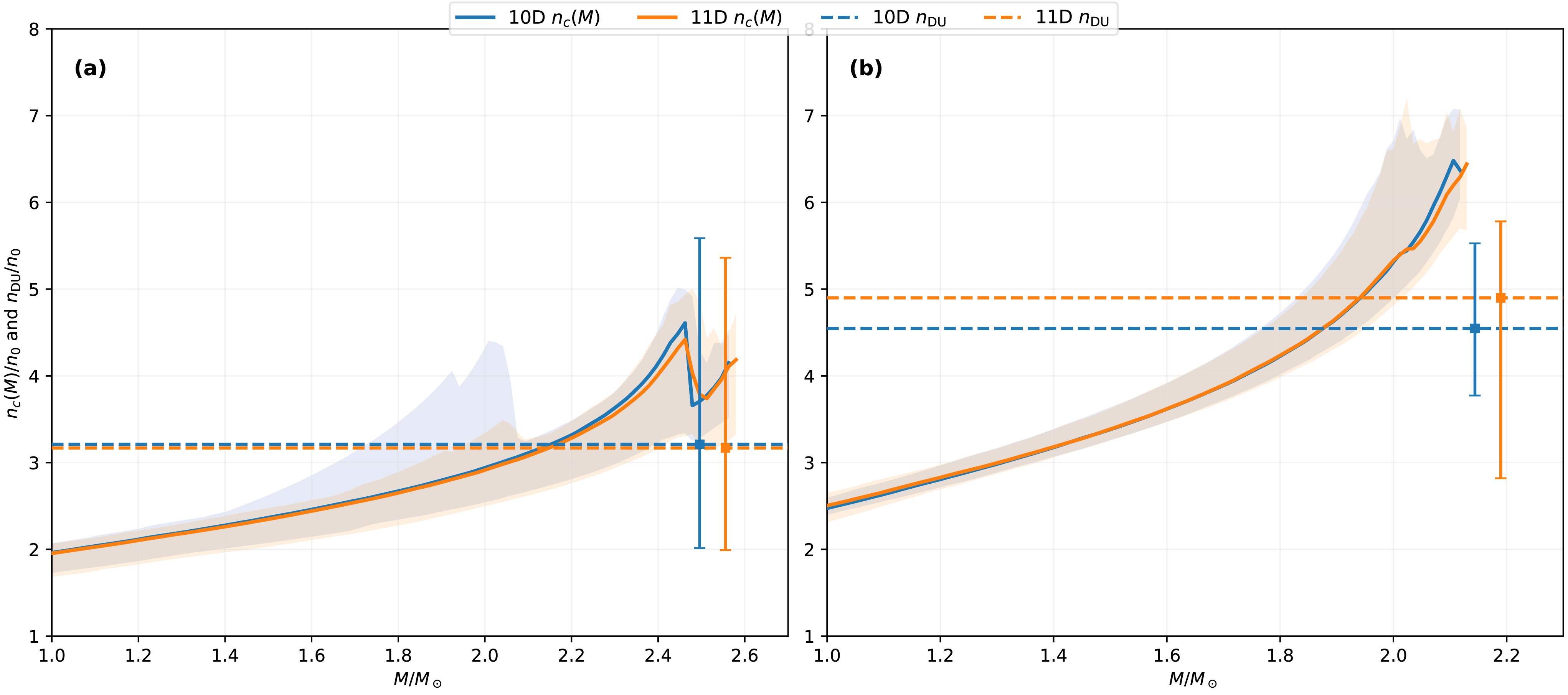
Figure 5. (color online) The central density
$ n_c(M) $ along the stable stellar branch is compared with the posterior direct-Urca threshold density$ n_{\rm{DU}} $ . Panel (a) shows the NS+GW results and panel (b) shows the ALL+GW results. Solid curves denote the representative posterior prediction for$ n_c(M)/n_0 $ , while dashed horizontal lines indicate the corresponding representative value of$ n_{\rm{DU}}/n_0 $ . The shaded bands show the 90% posterior uncertainty. The square markers with vertical error bars show the same representative$ n_{\rm{DU}}/n_0 $ values and their 90% HPD intervals from the corresponding summary table. They are placed near the high-mass end of the corresponding posterior stellar sequences solely to indicate the threshold-density uncertainty; they are not additional observational data.The corresponding posterior summaries of the high-density isovector and direct-Urca quantities are listed in the following table. The table includes
$ E_{\rm{sym}}(2n_0) $ ,$ E_{\rm{sym}}(3n_0) $ ,$ Y_p(2n_0) $ ,$ Y_p(3n_0) $ ,$ n_{\rm{DU}}/n_0 $ , and$ M_{\rm{DU}} $ . Here$ M_{\rm{DU}} $ is defined as the stellar mass for which the stable branch first reaches$ n_c(M)=n_{\rm{DU}} $ . If the direct-Urca threshold is not reached on the stable branch, the corresponding sample is treated as a right-censored no-onset sample; the finite-onset$ M_{\rm{DU}} $ summary and the no-onset probability are reported separately below. The comparison between 10D and 11D shows how the additional ρ-channel flexibility propagates from the symmetry energy to the proton fraction and then to the direct-Urca threshold.To express the direct-Urca onset in a mass-dependent form, we define the direct-Urca activation probability
$ P_{\rm{DU}}(M) = {\rm{Prob}}\left[ n_c(M)\ge n_{\rm{DU}} \,\middle|\, M_{\max}\ge M \right]. $
(40) The condition
$ M_{\max}\ge M $ restricts the probability to posterior samples that support a stable star of mass M. This definition avoids counting samples for which the stellar model does not exist at the specified mass. The activation probability therefore gives the posterior probability that a star of mass M contains a core region where the direct-Urca process is kinematically allowed.Figure 6 shows
$ P_{\rm{DU}}(M) $ for the 10D baseline and 11D ρ-flex models. As expected, the activation probability generally increases with stellar mass because the central density rises along the stable branch. The comparison between 10D and 11D converts the difference in$ n_{\rm{DU}} $ into a mass-dependent quantity. This quantity is directly related to the fast-cooling channel, although a full cooling calculation would also require neutrino emissivities, superfluid gaps, envelope composition, and thermal evolution modeling [35, 36, 81]. In the present analysis,$ P_{\rm{DU}}(M) $ is used only as a composition-sensitive diagnostic derived from the EOS posterior. Because$ P_{\rm{DU}}(M) $ is conditioned on$ M_{\max}\ge M $ , the ensemble used in the denominator changes with M. Near the high-mass end, where only a small subset of posterior samples still supports a stable star, this conditional normalization and finite sampling can produce small nonmonotonic features, such as the drop visible in Fig. 6(a). This feature should not be interpreted as a physical decrease of the direct-Urca probability along an individual stellar sequence; for any fixed EOS, once the central density exceeds$ n_{\rm{DU}} $ , the direct-Urca channel remains open at larger central densities on the stable branch. To check this explicitly, we monitored the effective number of posterior samples entering the denominator, denoted by$ N_{\rm{eff}}(M) $ . Here$ N_{\rm{eff}}(M) $ is simply the number of samples for which$ M_{\max}\ge M $ and the interpolated central density$ n_c(M) $ is finite. In the NS+GW panel of Fig. 6,$ N_{\rm{eff}} $ remains close to the full plotted sample size through the well-populated mass range, but decreases rapidly at the extreme high-mass endpoint. For example, in the posterior sample set used for this diagnostic$ N_{\rm{eff}}=80 $ at$ M=2.0M_\odot $ , remains about$ 75 $ –$ 76 $ at$ M=2.4M_\odot $ , and then falls to only a few samples near the endpoint of the 10D and 11D curves. Thus the visible non-smooth behavior is caused by conditional normalization and finite posterior sampling near the edge of the supported mass range, not by a discontinuity in the EOS or by a physical closing of the direct-Urca channel.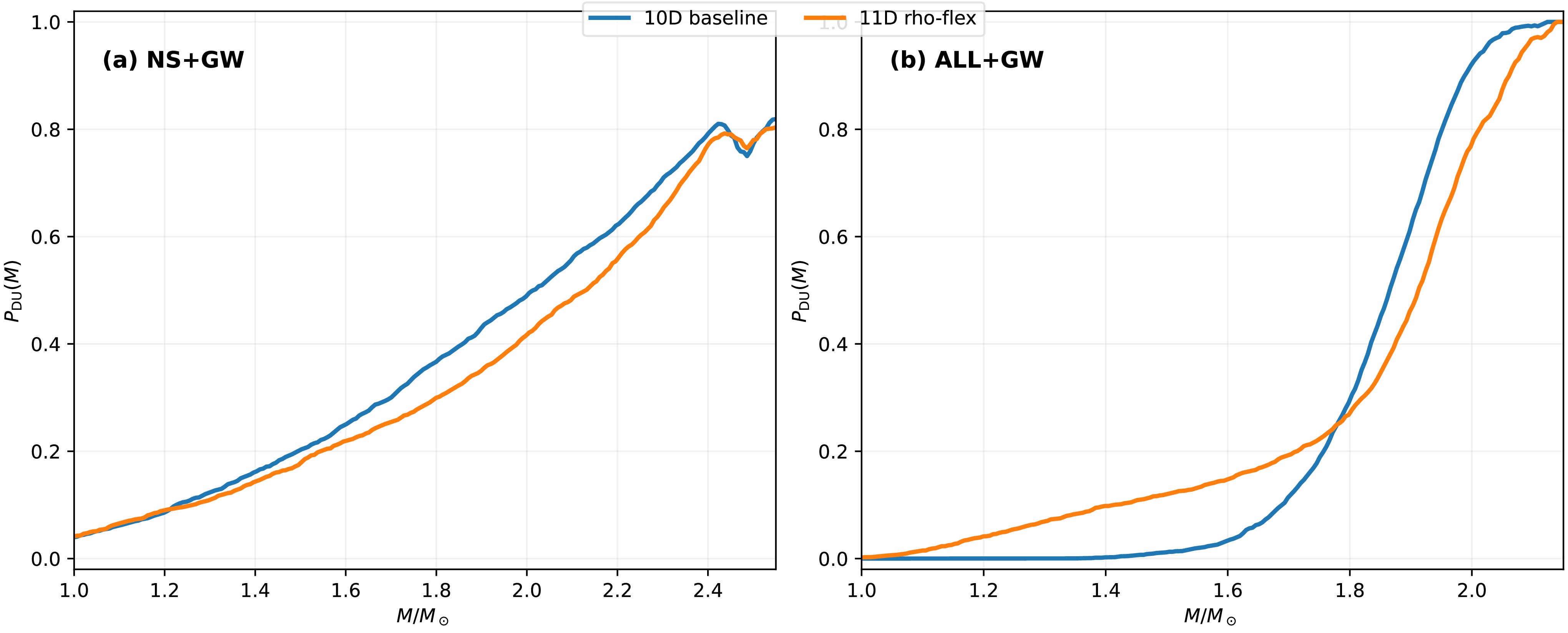
Figure 6. (color online) The direct-Urca activation probability as a function of stellar mass is
$ P_{\rm{DU}}(M)= {\rm{Prob}} \left[n_c(M)\ge n_{\rm{DU}}\mid M_{\max}\ge M\right] $ . Panel (a) shows the NS+GW result, and panel (b) shows the ALL+GW result. Small non-monotonic features near the high-mass end arise from changes in the set of posterior samples satisfying$ M_{\max}\ge M $ and from finite sampling, not from a closure of the direct-Urca channel. Interpretation of the endpoint behavior is limited by the rapid decrease in the effective number of posterior samples in that mass range.The representative direct-Urca onset probabilities are listed in Table 5. Instead of presenting the mass-dependent activation probability
$ P_{\rm{DU}}(M) $ directly, we report the cumulative posterior distribution of the onset mass,$ P(M_{\rm{DU}}<M_{\rm{cut}}) $ , evaluated at representative mass thresholds$ M_{\rm{cut}} $ . This quantity gives the posterior probability that the direct-Urca process starts below a specified stellar mass. It provides a compact summary of the$ M_{\rm{DU}} $ posterior and is complementary to the mass-dependent activation probability shown in Fig. 6. Samples for which the direct-Urca threshold is not reached anywhere on the stable branch are treated as right-censored rather than discarded. We therefore also reportData set Model $ P_{\rm{no\,DU}} $ $ P(M_{\rm{DU}}<1.4M_\odot) $ $ P(M_{\rm{DU}}<1.6M_\odot) $ $ P(M_{\rm{DU}}<1.8M_\odot) $ $ P(M_{\rm{DU}}<2.0M_\odot) $ NS+GW 10D $ 3.6 $ $ 14.7 $ $ 23.7 $ $ 34.7 $ $ 48.8 $ NS+GW 11D $ 4.3 $ $ 17.8 $ $ 24.1 $ $ 31.6 $ $ 43.0 $ ALL+GW 10D $ 0.0 $ $ 0.0 $ $ 3.3 $ $ 29.1 $ $ 92.1 $ ALL+GW 11D $ 0.0 $ $ 7.9 $ $ 12.9 $ $ 23.2 $ $ 78.2 $ Table 5. Posterior probability (in percent) that the direct-Urca onset mass lies below representative mass thresholds, treating no-onset samples as right-censored. The column
$ P_{\rm{no\,DU}} $ gives the posterior probability that the direct-Urca threshold is not reached anywhere on the stable branch.$ P_{\rm no\,DU}={\rm{Prob}}\left[n_c(M)<n_{\rm{DU}}\ {\rm{for\ all\ stable}}\ M\right]. $
The probabilities
$ P(M_{\rm{DU}}<M_{\rm{cut}}) $ in Table 5 are evaluated unconditionally, counting no-onset samples as not satisfying any finite onset-mass cut. -
We next examine how the high-density isovector uncertainty affects the direct-Urca threshold. The nucleonic direct-Urca process,
$ n\rightarrow p+l+\bar{\nu}_l, \qquad p+l\rightarrow n+\nu_l, \qquad l=e,\mu , $
(39) is kinematically allowed when the Fermi momenta satisfy the triangle condition in Eq. (36). For a given EOS, this condition defines the direct-Urca threshold density
$ n_{\rm{DU}} $ . If the central density of a star of mass M, denoted$ n_c(M) $ , exceeds this threshold, the direct-Urca channel is open in the stellar core.Figure 5 compares the posterior central-density curves
$ n_c(M) $ with the corresponding direct-Urca threshold density$ n_{\rm{DU}} $ . The results are shown separately for NS+GW and ALL+GW. For each model, the stellar sequence determines$ n_c(M) $ , while the composition of beta-equilibrated matter determines$ n_{\rm{DU}} $ . Thus, the onset of direct Urca in a star of mass M depends on the relative position of these two quantities. The 10D and 11D models can have similar central-density curves because their bulk beta-equilibrium pressures are similar, but they can still differ in$ n_{\rm{DU}} $ through their different high-density proton fractions. The difference between the 10D and 11D direct-Urca thresholds is more visible for ALL+GW than for NS+GW. For NS+GW, the high-density isovector sector is only weakly constrained by the mass-radius and tidal data, and the allowed ranges of L,$ K_{\rm{sym}} $ , and$ f_{\rho,\infty} $ already generate a broad spread of$ E_{\rm{sym}}(n) $ ,$ Y_p(n) $ , and$ n_{\rm{DU}} $ within the 10D baseline. Consequently, the additional ρ-channel flexibility in the 11D model mostly broadens an already wide threshold distribution, and the 10D and 11D$ n_{\rm{DU}} $ intervals strongly overlap. For ALL+GW, the additional χEFT and HIC constraints restrict the low- and intermediate-density EOS and reduce part of the 10D posterior freedom. After this compression of the baseline model space, the residual high-density ρ-channel deformation in the 11D model produces a more visible shift in the representative$ n_{\rm{DU}} $ , even though the 10D and 11D HPD intervals still overlap. This behavior reflects the fact that$ n_c(M) $ is mainly controlled by the bulk pressure, whereas$ n_{\rm{DU}} $ is controlled by the composition through the proton fraction. The apparent high-mass bends in$ n_c(M) $ , especially near the end of the NS+GW sequences in Fig. 5(a), have the same origin as the high-mass behavior of the$ M - R $ bands: the stable branch is approaching$ M_{\max} $ , and the posterior sample set contributing to the plotted representative curve and band changes rapidly. They are therefore endpoint and sampling effects rather than abrupt changes of the underlying EOS.
Figure 5. (color online) The central density
$ n_c(M) $ along the stable stellar branch is compared with the posterior direct-Urca threshold density$ n_{\rm{DU}} $ . Panel (a) shows the NS+GW results and panel (b) shows the ALL+GW results. Solid curves denote the representative posterior prediction for$ n_c(M)/n_0 $ , while dashed horizontal lines indicate the corresponding representative value of$ n_{\rm{DU}}/n_0 $ . The shaded bands show the 90% posterior uncertainty. The square markers with vertical error bars show the same representative$ n_{\rm{DU}}/n_0 $ values and their 90% HPD intervals from the corresponding summary table. They are placed near the high-mass end of the corresponding posterior stellar sequences solely to indicate the threshold-density uncertainty; they are not additional observational data.The corresponding posterior summaries of the high-density isovector and direct-Urca quantities are listed in the following table. The table includes
$ E_{\rm{sym}}(2n_0) $ ,$ E_{\rm{sym}}(3n_0) $ ,$ Y_p(2n_0) $ ,$ Y_p(3n_0) $ ,$ n_{\rm{DU}}/n_0 $ , and$ M_{\rm{DU}} $ . Here$ M_{\rm{DU}} $ is defined as the stellar mass for which the stable branch first reaches$ n_c(M)=n_{\rm{DU}} $ . If the direct-Urca threshold is not reached on the stable branch, the corresponding sample is treated as a right-censored no-onset sample; the finite-onset$ M_{\rm{DU}} $ summary and the no-onset probability are reported separately below. The comparison between 10D and 11D shows how the additional ρ-channel flexibility propagates from the symmetry energy to the proton fraction and then to the direct-Urca threshold.To express the direct-Urca onset in a mass-dependent form, we define the direct-Urca activation probability
$ P_{\rm{DU}}(M) = {\rm{Prob}}\left[ n_c(M)\ge n_{\rm{DU}} \,\middle|\, M_{\max}\ge M \right]. $
(40) The condition
$ M_{\max}\ge M $ restricts the probability to posterior samples that support a stable star of mass M. This definition avoids counting samples for which the stellar model does not exist at the specified mass. The activation probability therefore gives the posterior probability that a star of mass M contains a core region where the direct-Urca process is kinematically allowed.Figure 6 shows
$ P_{\rm{DU}}(M) $ for the 10D baseline and 11D ρ-flex models. As expected, the activation probability generally increases with stellar mass because the central density rises along the stable branch. The comparison between 10D and 11D converts the difference in$ n_{\rm{DU}} $ into a mass-dependent quantity. This quantity is directly related to the fast-cooling channel, although a full cooling calculation would also require neutrino emissivities, superfluid gaps, envelope composition, and thermal evolution modeling [35, 36, 81]. In the present analysis,$ P_{\rm{DU}}(M) $ is used only as a composition-sensitive diagnostic derived from the EOS posterior. Because$ P_{\rm{DU}}(M) $ is conditioned on$ M_{\max}\ge M $ , the ensemble used in the denominator changes with M. Near the high-mass end, where only a small subset of posterior samples still supports a stable star, this conditional normalization and finite sampling can produce small nonmonotonic features, such as the drop visible in Fig. 6(a). This feature should not be interpreted as a physical decrease of the direct-Urca probability along an individual stellar sequence; for any fixed EOS, once the central density exceeds$ n_{\rm{DU}} $ , the direct-Urca channel remains open at larger central densities on the stable branch. To check this explicitly, we monitored the effective number of posterior samples entering the denominator, denoted by$ N_{\rm{eff}}(M) $ . Here$ N_{\rm{eff}}(M) $ is simply the number of samples for which$ M_{\max}\ge M $ and the interpolated central density$ n_c(M) $ is finite. In the NS+GW panel of Fig. 6,$ N_{\rm{eff}} $ remains close to the full plotted sample size through the well-populated mass range, but decreases rapidly at the extreme high-mass endpoint. For example, in the posterior sample set used for this diagnostic$ N_{\rm{eff}}=80 $ at$ M=2.0M_\odot $ , remains about$ 75 $ –$ 76 $ at$ M=2.4M_\odot $ , and then falls to only a few samples near the endpoint of the 10D and 11D curves. Thus the visible non-smooth behavior is caused by conditional normalization and finite posterior sampling near the edge of the supported mass range, not by a discontinuity in the EOS or by a physical closing of the direct-Urca channel.
Figure 6. (color online) The direct-Urca activation probability as a function of stellar mass is
$ P_{\rm{DU}}(M)= {\rm{Prob}} \left[n_c(M)\ge n_{\rm{DU}}\mid M_{\max}\ge M\right] $ . Panel (a) shows the NS+GW result, and panel (b) shows the ALL+GW result. Small non-monotonic features near the high-mass end arise from changes in the set of posterior samples satisfying$ M_{\max}\ge M $ and from finite sampling, not from a closure of the direct-Urca channel. Interpretation of the endpoint behavior is limited by the rapid decrease in the effective number of posterior samples in that mass range.The representative direct-Urca onset probabilities are listed in Table 5. Instead of presenting the mass-dependent activation probability
$ P_{\rm{DU}}(M) $ directly, we report the cumulative posterior distribution of the onset mass,$ P(M_{\rm{DU}}<M_{\rm{cut}}) $ , evaluated at representative mass thresholds$ M_{\rm{cut}} $ . This quantity gives the posterior probability that the direct-Urca process starts below a specified stellar mass. It provides a compact summary of the$ M_{\rm{DU}} $ posterior and is complementary to the mass-dependent activation probability shown in Fig. 6. Samples for which the direct-Urca threshold is not reached anywhere on the stable branch are treated as right-censored rather than discarded. We therefore also reportData set Model $ P_{\rm{no\,DU}} $ $ P(M_{\rm{DU}}<1.4M_\odot) $ $ P(M_{\rm{DU}}<1.6M_\odot) $ $ P(M_{\rm{DU}}<1.8M_\odot) $ $ P(M_{\rm{DU}}<2.0M_\odot) $ NS+GW 10D $ 3.6 $ $ 14.7 $ $ 23.7 $ $ 34.7 $ $ 48.8 $ NS+GW 11D $ 4.3 $ $ 17.8 $ $ 24.1 $ $ 31.6 $ $ 43.0 $ ALL+GW 10D $ 0.0 $ $ 0.0 $ $ 3.3 $ $ 29.1 $ $ 92.1 $ ALL+GW 11D $ 0.0 $ $ 7.9 $ $ 12.9 $ $ 23.2 $ $ 78.2 $ Table 5. Posterior probability (in percent) that the direct-Urca onset mass lies below representative mass thresholds, treating no-onset samples as right-censored. The column
$ P_{\rm{no\,DU}} $ gives the posterior probability that the direct-Urca threshold is not reached anywhere on the stable branch.$ P_{\rm no\,DU}={\rm{Prob}}\left[n_c(M)<n_{\rm{DU}}\ {\rm{for\ all\ stable}}\ M\right]. $
The probabilities
$ P(M_{\rm{DU}}<M_{\rm{cut}}) $ in Table 5 are evaluated unconditionally, counting no-onset samples as not satisfying any finite onset-mass cut. -
We next examine how the high-density isovector uncertainty affects the direct-Urca threshold. The nucleonic direct-Urca process,
$ n\rightarrow p+l+\bar{\nu}_l, \qquad p+l\rightarrow n+\nu_l, \qquad l=e,\mu , $
(39) is kinematically allowed when the Fermi momenta satisfy the triangle condition in Eq. (36). For a given EOS, this condition defines the direct-Urca threshold density
$ n_{\rm{DU}} $ . If the central density of a star of mass M, denoted$ n_c(M) $ , exceeds this threshold, the direct-Urca channel is open in the stellar core.Figure 5 compares the posterior central-density curves
$ n_c(M) $ with the corresponding direct-Urca threshold density$ n_{\rm{DU}} $ . The results are shown separately for NS+GW and ALL+GW. For each model, the stellar sequence determines$ n_c(M) $ , while the composition of beta-equilibrated matter determines$ n_{\rm{DU}} $ . Thus, the onset of direct Urca in a star of mass M depends on the relative position of these two quantities. The 10D and 11D models can have similar central-density curves because their bulk beta-equilibrium pressures are similar, but they can still differ in$ n_{\rm{DU}} $ through their different high-density proton fractions. The difference between the 10D and 11D direct-Urca thresholds is more visible for ALL+GW than for NS+GW. For NS+GW, the high-density isovector sector is only weakly constrained by the mass-radius and tidal data, and the allowed ranges of L,$ K_{\rm{sym}} $ , and$ f_{\rho,\infty} $ already generate a broad spread of$ E_{\rm{sym}}(n) $ ,$ Y_p(n) $ , and$ n_{\rm{DU}} $ within the 10D baseline. Consequently, the additional ρ-channel flexibility in the 11D model mostly broadens an already wide threshold distribution, and the 10D and 11D$ n_{\rm{DU}} $ intervals strongly overlap. For ALL+GW, the additional χEFT and HIC constraints restrict the low- and intermediate-density EOS and reduce part of the 10D posterior freedom. After this compression of the baseline model space, the residual high-density ρ-channel deformation in the 11D model produces a more visible shift in the representative$ n_{\rm{DU}} $ , even though the 10D and 11D HPD intervals still overlap. This behavior reflects the fact that$ n_c(M) $ is mainly controlled by the bulk pressure, whereas$ n_{\rm{DU}} $ is controlled by the composition through the proton fraction. The apparent high-mass bends in$ n_c(M) $ , especially near the end of the NS+GW sequences in Fig. 5(a), have the same origin as the high-mass behavior of the$ M - R $ bands: the stable branch is approaching$ M_{\max} $ , and the posterior sample set contributing to the plotted representative curve and band changes rapidly. They are therefore endpoint and sampling effects rather than abrupt changes of the underlying EOS.
Figure 5. (color online) The central density
$ n_c(M) $ along the stable stellar branch is compared with the posterior direct-Urca threshold density$ n_{\rm{DU}} $ . Panel (a) shows the NS+GW results and panel (b) shows the ALL+GW results. Solid curves denote the representative posterior prediction for$ n_c(M)/n_0 $ , while dashed horizontal lines indicate the corresponding representative value of$ n_{\rm{DU}}/n_0 $ . The shaded bands show the 90% posterior uncertainty. The square markers with vertical error bars show the same representative$ n_{\rm{DU}}/n_0 $ values and their 90% HPD intervals from the corresponding summary table. They are placed near the high-mass end of the corresponding posterior stellar sequences solely to indicate the threshold-density uncertainty; they are not additional observational data.The corresponding posterior summaries of the high-density isovector and direct-Urca quantities are listed in the following table. The table includes
$ E_{\rm{sym}}(2n_0) $ ,$ E_{\rm{sym}}(3n_0) $ ,$ Y_p(2n_0) $ ,$ Y_p(3n_0) $ ,$ n_{\rm{DU}}/n_0 $ , and$ M_{\rm{DU}} $ . Here$ M_{\rm{DU}} $ is defined as the stellar mass for which the stable branch first reaches$ n_c(M)=n_{\rm{DU}} $ . If the direct-Urca threshold is not reached on the stable branch, the corresponding sample is treated as a right-censored no-onset sample; the finite-onset$ M_{\rm{DU}} $ summary and the no-onset probability are reported separately below. The comparison between 10D and 11D shows how the additional ρ-channel flexibility propagates from the symmetry energy to the proton fraction and then to the direct-Urca threshold.To express the direct-Urca onset in a mass-dependent form, we define the direct-Urca activation probability
$ P_{\rm{DU}}(M) = {\rm{Prob}}\left[ n_c(M)\ge n_{\rm{DU}} \,\middle|\, M_{\max}\ge M \right]. $
(40) The condition
$ M_{\max}\ge M $ restricts the probability to posterior samples that support a stable star of mass M. This definition avoids counting samples for which the stellar model does not exist at the specified mass. The activation probability therefore gives the posterior probability that a star of mass M contains a core region where the direct-Urca process is kinematically allowed.Figure 6 shows
$ P_{\rm{DU}}(M) $ for the 10D baseline and 11D ρ-flex models. As expected, the activation probability generally increases with stellar mass because the central density rises along the stable branch. The comparison between 10D and 11D converts the difference in$ n_{\rm{DU}} $ into a mass-dependent quantity. This quantity is directly related to the fast-cooling channel, although a full cooling calculation would also require neutrino emissivities, superfluid gaps, envelope composition, and thermal evolution modeling [35, 36, 81]. In the present analysis,$ P_{\rm{DU}}(M) $ is used only as a composition-sensitive diagnostic derived from the EOS posterior. Because$ P_{\rm{DU}}(M) $ is conditioned on$ M_{\max}\ge M $ , the ensemble used in the denominator changes with M. Near the high-mass end, where only a small subset of posterior samples still supports a stable star, this conditional normalization and finite sampling can produce small nonmonotonic features, such as the drop visible in Fig. 6(a). This feature should not be interpreted as a physical decrease of the direct-Urca probability along an individual stellar sequence; for any fixed EOS, once the central density exceeds$ n_{\rm{DU}} $ , the direct-Urca channel remains open at larger central densities on the stable branch. To check this explicitly, we monitored the effective number of posterior samples entering the denominator, denoted by$ N_{\rm{eff}}(M) $ . Here$ N_{\rm{eff}}(M) $ is simply the number of samples for which$ M_{\max}\ge M $ and the interpolated central density$ n_c(M) $ is finite. In the NS+GW panel of Fig. 6,$ N_{\rm{eff}} $ remains close to the full plotted sample size through the well-populated mass range, but decreases rapidly at the extreme high-mass endpoint. For example, in the posterior sample set used for this diagnostic$ N_{\rm{eff}}=80 $ at$ M=2.0M_\odot $ , remains about$ 75 $ –$ 76 $ at$ M=2.4M_\odot $ , and then falls to only a few samples near the endpoint of the 10D and 11D curves. Thus the visible non-smooth behavior is caused by conditional normalization and finite posterior sampling near the edge of the supported mass range, not by a discontinuity in the EOS or by a physical closing of the direct-Urca channel.
Figure 6. (color online) The direct-Urca activation probability as a function of stellar mass is
$ P_{\rm{DU}}(M)= {\rm{Prob}} \left[n_c(M)\ge n_{\rm{DU}}\mid M_{\max}\ge M\right] $ . Panel (a) shows the NS+GW result, and panel (b) shows the ALL+GW result. Small non-monotonic features near the high-mass end arise from changes in the set of posterior samples satisfying$ M_{\max}\ge M $ and from finite sampling, not from a closure of the direct-Urca channel. Interpretation of the endpoint behavior is limited by the rapid decrease in the effective number of posterior samples in that mass range.The representative direct-Urca onset probabilities are listed in Table 5. Instead of presenting the mass-dependent activation probability
$ P_{\rm{DU}}(M) $ directly, we report the cumulative posterior distribution of the onset mass,$ P(M_{\rm{DU}}<M_{\rm{cut}}) $ , evaluated at representative mass thresholds$ M_{\rm{cut}} $ . This quantity gives the posterior probability that the direct-Urca process starts below a specified stellar mass. It provides a compact summary of the$ M_{\rm{DU}} $ posterior and is complementary to the mass-dependent activation probability shown in Fig. 6. Samples for which the direct-Urca threshold is not reached anywhere on the stable branch are treated as right-censored rather than discarded. We therefore also reportData set Model $ P_{\rm{no\,DU}} $ $ P(M_{\rm{DU}}<1.4M_\odot) $ $ P(M_{\rm{DU}}<1.6M_\odot) $ $ P(M_{\rm{DU}}<1.8M_\odot) $ $ P(M_{\rm{DU}}<2.0M_\odot) $ NS+GW 10D $ 3.6 $ $ 14.7 $ $ 23.7 $ $ 34.7 $ $ 48.8 $ NS+GW 11D $ 4.3 $ $ 17.8 $ $ 24.1 $ $ 31.6 $ $ 43.0 $ ALL+GW 10D $ 0.0 $ $ 0.0 $ $ 3.3 $ $ 29.1 $ $ 92.1 $ ALL+GW 11D $ 0.0 $ $ 7.9 $ $ 12.9 $ $ 23.2 $ $ 78.2 $ Table 5. Posterior probability (in percent) that the direct-Urca onset mass lies below representative mass thresholds, treating no-onset samples as right-censored. The column
$ P_{\rm{no\,DU}} $ gives the posterior probability that the direct-Urca threshold is not reached anywhere on the stable branch.$ P_{\rm no\,DU}={\rm{Prob}}\left[n_c(M)<n_{\rm{DU}}\ {\rm{for\ all\ stable}}\ M\right]. $
The probabilities
$ P(M_{\rm{DU}}<M_{\rm{cut}}) $ in Table 5 are evaluated unconditionally, counting no-onset samples as not satisfying any finite onset-mass cut. -
We next examine how the high-density isovector uncertainty affects the direct-Urca threshold. The nucleonic direct-Urca process,
$ n\rightarrow p+l+\bar{\nu}_l, \qquad p+l\rightarrow n+\nu_l, \qquad l=e,\mu , $
(39) is kinematically allowed when the Fermi momenta satisfy the triangle condition in Eq. (36). For a given EOS, this condition defines the direct-Urca threshold density
$ n_{\rm{DU}} $ . If the central density of a star of mass M, denoted$ n_c(M) $ , exceeds this threshold, the direct-Urca channel is open in the stellar core.Figure 5 compares the posterior central-density curves
$ n_c(M) $ with the corresponding direct-Urca threshold density$ n_{\rm{DU}} $ . The results are shown separately for NS+GW and ALL+GW. For each model, the stellar sequence determines$ n_c(M) $ , while the composition of beta-equilibrated matter determines$ n_{\rm{DU}} $ . Thus, the onset of direct Urca in a star of mass M depends on the relative position of these two quantities. The 10D and 11D models can have similar central-density curves because their bulk beta-equilibrium pressures are similar, but they can still differ in$ n_{\rm{DU}} $ through their different high-density proton fractions. The difference between the 10D and 11D direct-Urca thresholds is more visible for ALL+GW than for NS+GW. For NS+GW, the high-density isovector sector is only weakly constrained by the mass-radius and tidal data, and the allowed ranges of L,$ K_{\rm{sym}} $ , and$ f_{\rho,\infty} $ already generate a broad spread of$ E_{\rm{sym}}(n) $ ,$ Y_p(n) $ , and$ n_{\rm{DU}} $ within the 10D baseline. Consequently, the additional ρ-channel flexibility in the 11D model mostly broadens an already wide threshold distribution, and the 10D and 11D$ n_{\rm{DU}} $ intervals strongly overlap. For ALL+GW, the additional χEFT and HIC constraints restrict the low- and intermediate-density EOS and reduce part of the 10D posterior freedom. After this compression of the baseline model space, the residual high-density ρ-channel deformation in the 11D model produces a more visible shift in the representative$ n_{\rm{DU}} $ , even though the 10D and 11D HPD intervals still overlap. This behavior reflects the fact that$ n_c(M) $ is mainly controlled by the bulk pressure, whereas$ n_{\rm{DU}} $ is controlled by the composition through the proton fraction. The apparent high-mass bends in$ n_c(M) $ , especially near the end of the NS+GW sequences in Fig. 5(a), have the same origin as the high-mass behavior of the$ M - R $ bands: the stable branch is approaching$ M_{\max} $ , and the posterior sample set contributing to the plotted representative curve and band changes rapidly. They are therefore endpoint and sampling effects rather than abrupt changes of the underlying EOS.
Figure 5. (color online) The central density
$ n_c(M) $ along the stable stellar branch is compared with the posterior direct-Urca threshold density$ n_{\rm{DU}} $ . Panel (a) shows the NS+GW results and panel (b) shows the ALL+GW results. Solid curves denote the representative posterior prediction for$ n_c(M)/n_0 $ , while dashed horizontal lines indicate the corresponding representative value of$ n_{\rm{DU}}/n_0 $ . The shaded bands show the 90% posterior uncertainty. The square markers with vertical error bars show the same representative$ n_{\rm{DU}}/n_0 $ values and their 90% HPD intervals from the corresponding summary table. They are placed near the high-mass end of the corresponding posterior stellar sequences solely to indicate the threshold-density uncertainty; they are not additional observational data.The corresponding posterior summaries of the high-density isovector and direct-Urca quantities are listed in the following table. The table includes
$ E_{\rm{sym}}(2n_0) $ ,$ E_{\rm{sym}}(3n_0) $ ,$ Y_p(2n_0) $ ,$ Y_p(3n_0) $ ,$ n_{\rm{DU}}/n_0 $ , and$ M_{\rm{DU}} $ . Here$ M_{\rm{DU}} $ is defined as the stellar mass for which the stable branch first reaches$ n_c(M)=n_{\rm{DU}} $ . If the direct-Urca threshold is not reached on the stable branch, the corresponding sample is treated as a right-censored no-onset sample; the finite-onset$ M_{\rm{DU}} $ summary and the no-onset probability are reported separately below. The comparison between 10D and 11D shows how the additional ρ-channel flexibility propagates from the symmetry energy to the proton fraction and then to the direct-Urca threshold.To express the direct-Urca onset in a mass-dependent form, we define the direct-Urca activation probability
$ P_{\rm{DU}}(M) = {\rm{Prob}}\left[ n_c(M)\ge n_{\rm{DU}} \,\middle|\, M_{\max}\ge M \right]. $
(40) The condition
$ M_{\max}\ge M $ restricts the probability to posterior samples that support a stable star of mass M. This definition avoids counting samples for which the stellar model does not exist at the specified mass. The activation probability therefore gives the posterior probability that a star of mass M contains a core region where the direct-Urca process is kinematically allowed.Figure 6 shows
$ P_{\rm{DU}}(M) $ for the 10D baseline and 11D ρ-flex models. As expected, the activation probability generally increases with stellar mass because the central density rises along the stable branch. The comparison between 10D and 11D converts the difference in$ n_{\rm{DU}} $ into a mass-dependent quantity. This quantity is directly related to the fast-cooling channel, although a full cooling calculation would also require neutrino emissivities, superfluid gaps, envelope composition, and thermal evolution modeling [35, 36, 81]. In the present analysis,$ P_{\rm{DU}}(M) $ is used only as a composition-sensitive diagnostic derived from the EOS posterior. Because$ P_{\rm{DU}}(M) $ is conditioned on$ M_{\max}\ge M $ , the ensemble used in the denominator changes with M. Near the high-mass end, where only a small subset of posterior samples still supports a stable star, this conditional normalization and finite sampling can produce small nonmonotonic features, such as the drop visible in Fig. 6(a). This feature should not be interpreted as a physical decrease of the direct-Urca probability along an individual stellar sequence; for any fixed EOS, once the central density exceeds$ n_{\rm{DU}} $ , the direct-Urca channel remains open at larger central densities on the stable branch. To check this explicitly, we monitored the effective number of posterior samples entering the denominator, denoted by$ N_{\rm{eff}}(M) $ . Here$ N_{\rm{eff}}(M) $ is simply the number of samples for which$ M_{\max}\ge M $ and the interpolated central density$ n_c(M) $ is finite. In the NS+GW panel of Fig. 6,$ N_{\rm{eff}} $ remains close to the full plotted sample size through the well-populated mass range, but decreases rapidly at the extreme high-mass endpoint. For example, in the posterior sample set used for this diagnostic$ N_{\rm{eff}}=80 $ at$ M=2.0M_\odot $ , remains about$ 75 $ –$ 76 $ at$ M=2.4M_\odot $ , and then falls to only a few samples near the endpoint of the 10D and 11D curves. Thus the visible non-smooth behavior is caused by conditional normalization and finite posterior sampling near the edge of the supported mass range, not by a discontinuity in the EOS or by a physical closing of the direct-Urca channel.
Figure 6. (color online) The direct-Urca activation probability as a function of stellar mass is
$ P_{\rm{DU}}(M)= {\rm{Prob}} \left[n_c(M)\ge n_{\rm{DU}}\mid M_{\max}\ge M\right] $ . Panel (a) shows the NS+GW result, and panel (b) shows the ALL+GW result. Small non-monotonic features near the high-mass end arise from changes in the set of posterior samples satisfying$ M_{\max}\ge M $ and from finite sampling, not from a closure of the direct-Urca channel. Interpretation of the endpoint behavior is limited by the rapid decrease in the effective number of posterior samples in that mass range.The representative direct-Urca onset probabilities are listed in Table 5. Instead of presenting the mass-dependent activation probability
$ P_{\rm{DU}}(M) $ directly, we report the cumulative posterior distribution of the onset mass,$ P(M_{\rm{DU}}<M_{\rm{cut}}) $ , evaluated at representative mass thresholds$ M_{\rm{cut}} $ . This quantity gives the posterior probability that the direct-Urca process starts below a specified stellar mass. It provides a compact summary of the$ M_{\rm{DU}} $ posterior and is complementary to the mass-dependent activation probability shown in Fig. 6. Samples for which the direct-Urca threshold is not reached anywhere on the stable branch are treated as right-censored rather than discarded. We therefore also reportData set Model $ P_{\rm{no\,DU}} $ $ P(M_{\rm{DU}}<1.4M_\odot) $ $ P(M_{\rm{DU}}<1.6M_\odot) $ $ P(M_{\rm{DU}}<1.8M_\odot) $ $ P(M_{\rm{DU}}<2.0M_\odot) $ NS+GW 10D $ 3.6 $ $ 14.7 $ $ 23.7 $ $ 34.7 $ $ 48.8 $ NS+GW 11D $ 4.3 $ $ 17.8 $ $ 24.1 $ $ 31.6 $ $ 43.0 $ ALL+GW 10D $ 0.0 $ $ 0.0 $ $ 3.3 $ $ 29.1 $ $ 92.1 $ ALL+GW 11D $ 0.0 $ $ 7.9 $ $ 12.9 $ $ 23.2 $ $ 78.2 $ Table 5. Posterior probability (in percent) that the direct-Urca onset mass lies below representative mass thresholds, treating no-onset samples as right-censored. The column
$ P_{\rm{no\,DU}} $ gives the posterior probability that the direct-Urca threshold is not reached anywhere on the stable branch.$ P_{\rm no\,DU}={\rm{Prob}}\left[n_c(M)<n_{\rm{DU}}\ {\rm{for\ all\ stable}}\ M\right]. $
The probabilities
$ P(M_{\rm{DU}}<M_{\rm{cut}}) $ in Table 5 are evaluated unconditionally, counting no-onset samples as not satisfying any finite onset-mass cut. -
We finally examine the posterior correlations in the 11D ρ-flex model. To keep the main text readable, we show the two most relevant ALL+GW corner plots in this section and place the corresponding NS+GW parameter/isovector plots, together with the selected macroscopic-observable corner plot, in Appendix A. The corner plots use consistent colors, line styles, diagonal annotations, and label positions across the main text and appendix. Figure 7 shows the parameter posteriors for the ALL+ GW data set. The diagonal panels display the one-dimensional marginalized posteriors of the 11D model parameters. For the ten parameters common to the 10D and 11D models, the corresponding 10D one-dimensional posteriors are overlaid on the diagonal panels. The off-diagonal panels show the two-dimensional posterior contours of the 11D model. This representation reveals the correlations between the additional ρ-channel parameter
$ \xi_\rho $ and the standard saturation and high-density control parameters.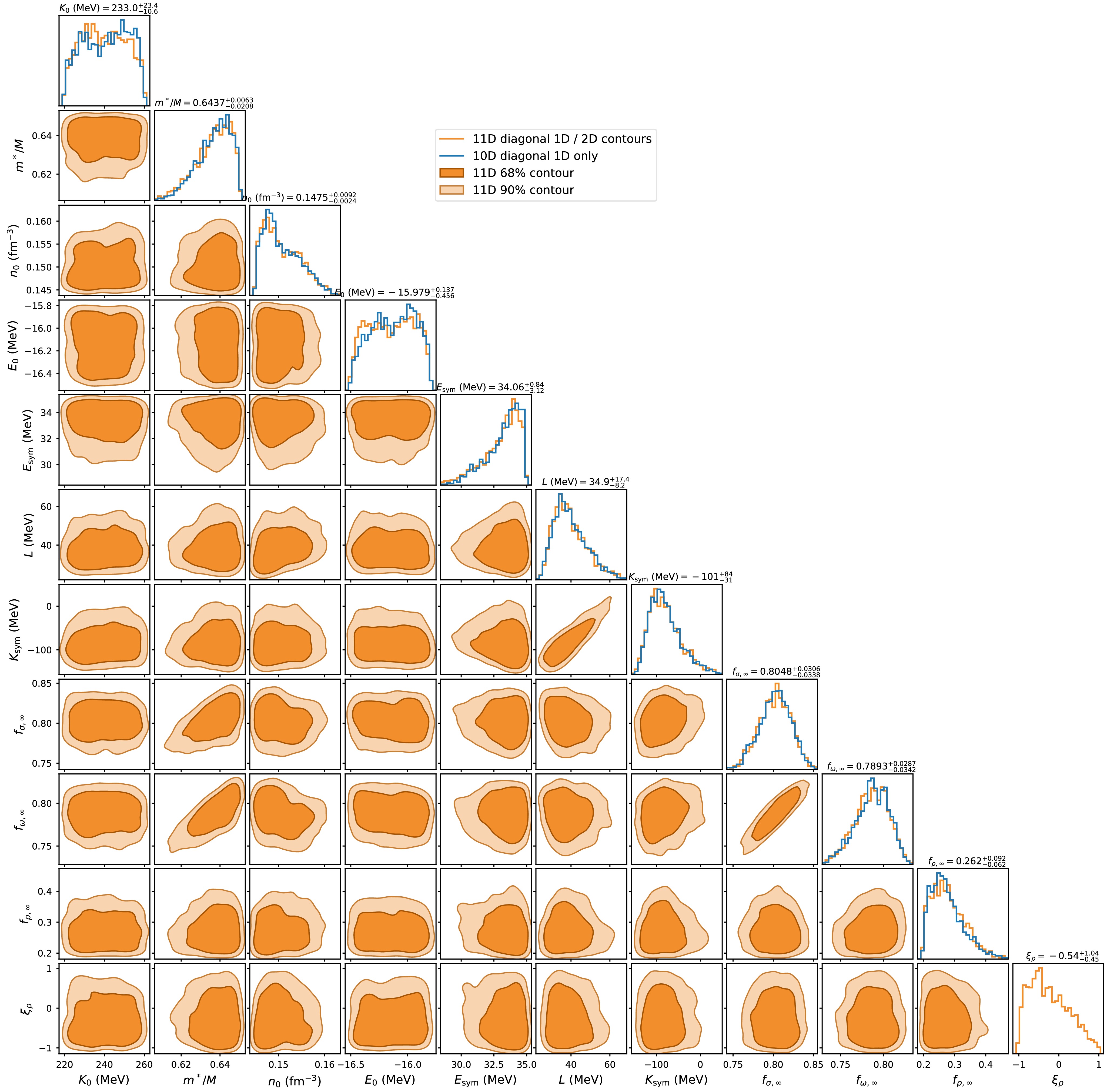
Figure 7. (color online) Posterior distributions of the 11D (ρ)-flex model parameters and their correlations for the ALL+GW data set are shown. For the 10 parameters common to both model spaces, the 10D baseline posterior is overlaid on the diagonal for comparison. The diagonal annotations indicate the posterior mode and the 90% credible intervals.
The parameter correlation plot shows that
$ \xi_\rho $ is not strongly constrained by the ALL+GW data alone. This is consistent with the evidence comparison in Table 2, which indicates no decisive preference for either the 10D baseline or the 11D extension. The posterior distribution of$ \xi_\rho $ therefore reflects the remaining freedom in the high-density ρ-channel that is not removed by the present combination of neutron-star, gravitational-wave, χEFT, and heavy-ion constraints. The comparison with the 10D diagonal posteriors also shows that introducing$ \xi_\rho $ does not strongly alter the marginalized distributions of most common bulk parameters.Figure 8 shows the corresponding corner plot for selected isovector and direct-Urca observables in the ALL+GW data set. The displayed quantities include
$ \xi_\rho $ , L,$ K_{\rm{sym}} $ ,$ E_{\rm{sym}}(2n_0) $ ,$ E_{\rm{sym}}(3n_0) $ ,$ Y_p(2n_0) $ ,$ Y_p(3n_0) $ ,$ n_{\rm{DU}}/n_0 $ , and$ M_{\rm{DU}} $ . The diagonal panels compare the one-dimensional posterior distributions of the 10D and 11D models where applicable, while the off-diagonal panels show the 11D correlations. This figure directly illustrates how the additional ρ-channel freedom propagates into high-density composition-sensitive quantities. The correlations in Fig. 8 are consistent with the posterior summaries in Table 6. The numerical entries are derived from the same posterior samples that produced the corresponding corner plots; therefore, the table and these figures are based on identical data and are mutually consistent. For ALL+GW, the 10D baseline yields relatively narrow intervals for$ E_{\rm{sym}}(3n_0) $ ,$ Y_p(3n_0) $ ,$ n_{\rm{DU}}/n_0 $ , and$ M_{\rm{DU}} $ . When the ρ-channel flexibility is introduced, the 11D model permits a broader range of these quantities. For example, Table 6 shows that the 11D ALL+GW result gives wider intervals for$ E_{\rm{sym}}(3n_0) $ ,$ Y_p(3n_0) $ , and$ M_{\rm{DU}} $ than the corresponding 10D result. The broader 11D intervals indicate that part of the apparent precision of the 10D prediction is conditional on the fixed high-density ρ-channel ansatz. In view of the small information gain of$ \xi_\rho $ reported in Sec. IIIB, this broadening is not interpreted as evidence that the present data favor a nonzero ρ-channel deformation. It mainly reflects the residual high-density isovector freedom allowed by the adopted 11D prior after the current data have constrained the bulk EOS.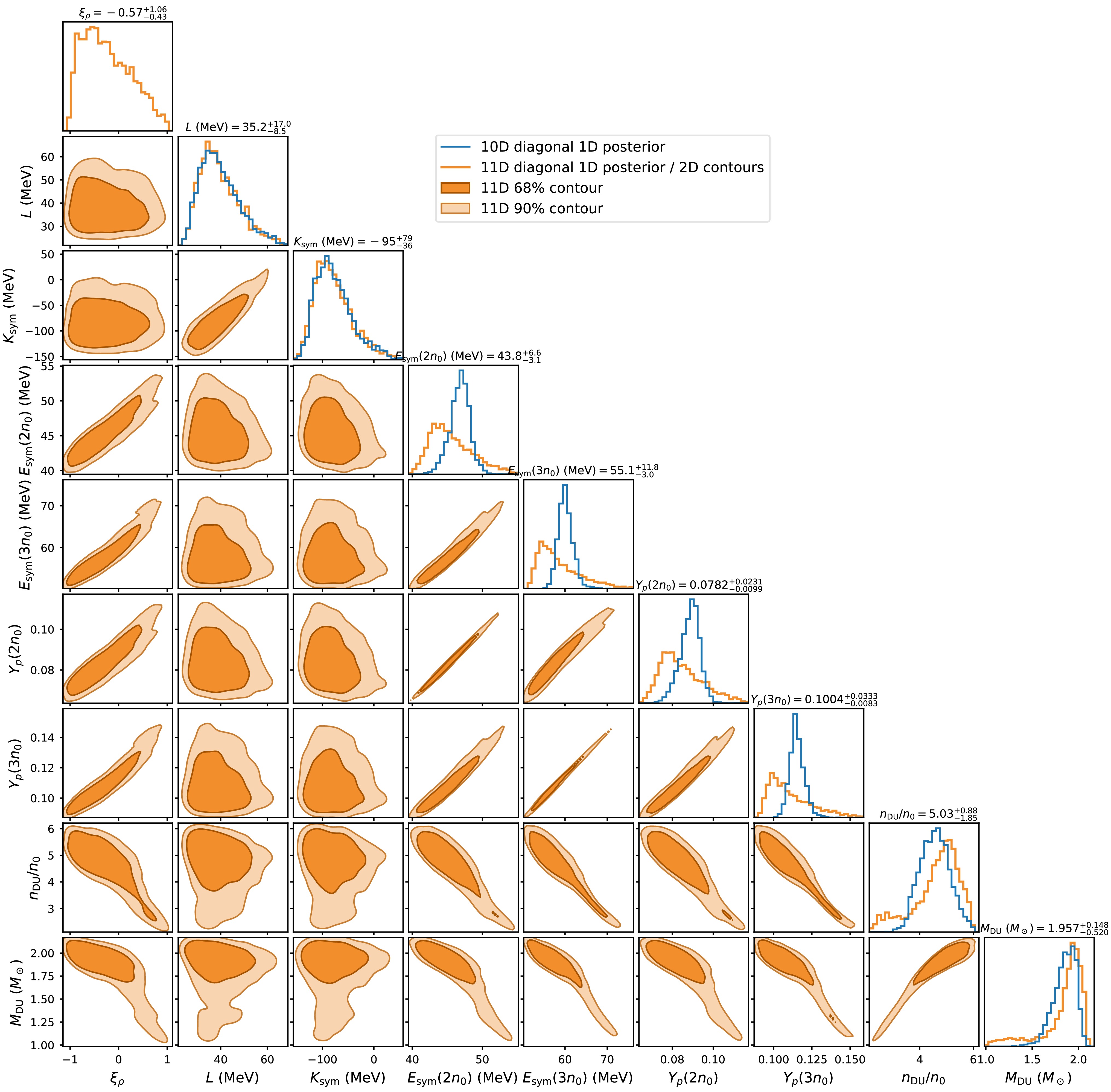
Figure 8. (color online) Corner plot of high-density isovector and direct Urca observables in the ALL+GW data set. The displayed quantities include
$ \xi_\rho $ , L,$ K_{\rm{sym}} $ ,$ E_{\rm{sym}}(2n_0) $ ,$ E_{\rm{sym}}(3n_0) $ ,$ Y_p(2n_0) $ ,$ Y_p(3n_0) $ ,$ n_{\rm{DU}}/n_0 $ , and$ M_{\rm{DU}} $ . The diagonal panels display the one-dimensional posterior distributions, overlaid with the 10D baseline results where applicable. The off-diagonal contours show the 11D posterior correlations.Data set Model $ E_{\rm{sym}}(2n_0) $ $ E_{\rm{sym}}(3n_0) $ $ Y_p(2n_0) $ $ Y_p(3n_0) $ $ n_{\rm{DU}}/n_0 $ $ M_{\rm{DU}} $ MeV MeV $ M_\odot $ NS+GW 10D $ 53.1^{+8.9}_{-6.5} $ $ 64.3^{+18.2}_{-5.4} $ $ 0.108^{+0.029}_{-0.021} $ $ 0.126^{+0.046}_{-0.014} $ $ 2.44^{+2.35}_{-0.70} $ $ 2.363^{+0.132}_{-1.242} $ NS+GW 11D $ 52.1^{+10.0}_{-6.8} $ $ 64.4^{+19.0}_{-7.1} $ $ 0.104^{+0.032}_{-0.023} $ $ 0.128^{+0.046}_{-0.021} $ $ 3.01^{+1.66}_{-1.32} $ $ 2.364^{+0.133}_{-1.290} $ ALL+GW 10D $ 47.0^{+2.0}_{-2.6} $ $ 59.8^{+3.3}_{-2.3} $ $ 0.090^{+0.006}_{-0.010} $ $ 0.115^{+0.008}_{-0.007} $ $ 4.62^{+0.78}_{-1.02} $ $ 1.929^{+0.103}_{-0.261} $ ALL+GW 11D $ 43.8^{+6.6}_{-3.1} $ $ 55.1^{+11.8}_{-3.1} $ $ 0.078^{+0.023}_{-0.010} $ $ 0.100^{+0.033}_{-0.008} $ $ 5.03^{+0.88}_{-1.85} $ $ 1.956^{+0.149}_{-0.519} $ Table 6. Posterior summaries of high-density isovector and direct-Urca observables. Entries list the posterior mode and the 90% HPD interval. For
$ M_{\rm{DU}} $ , the one-dimensional summary is reported for the finite-onset subset, while the posterior probability of no direct-Urca onset on the stable branch is reported separately in Table 5.The main role of Fig. 8 is therefore complementary to that of Figs. 3–6. The posterior predictive figures show that the bulk stellar observables are similar in the 10D and 11D models, whereas the isovector/DU corner plot reveals where the additional freedom appears in the composition-sensitive sector. Thus, the posterior correlation analysis supports the interpretation of
$ \xi_\rho $ as a controlled high-density isovector model-uncertainty parameter rather than as a parameter that primarily alters the bulk neutron-star structure. -
We finally examine the posterior correlations in the 11D ρ-flex model. To keep the main text readable, we show the two most relevant ALL+GW corner plots in this section and place the corresponding NS+GW parameter/isovector plots, together with the selected macroscopic-observable corner plot, in Appendix A. The corner plots use consistent colors, line styles, diagonal annotations, and label positions across the main text and appendix. Figure 7 shows the parameter posteriors for the ALL+ GW data set. The diagonal panels display the one-dimensional marginalized posteriors of the 11D model parameters. For the ten parameters common to the 10D and 11D models, the corresponding 10D one-dimensional posteriors are overlaid on the diagonal panels. The off-diagonal panels show the two-dimensional posterior contours of the 11D model. This representation reveals the correlations between the additional ρ-channel parameter
$ \xi_\rho $ and the standard saturation and high-density control parameters.
Figure 7. (color online) Posterior distributions of the 11D (ρ)-flex model parameters and their correlations for the ALL+GW data set are shown. For the 10 parameters common to both model spaces, the 10D baseline posterior is overlaid on the diagonal for comparison. The diagonal annotations indicate the posterior mode and the 90% credible intervals.
The parameter correlation plot shows that
$ \xi_\rho $ is not strongly constrained by the ALL+GW data alone. This is consistent with the evidence comparison in Table 2, which indicates no decisive preference for either the 10D baseline or the 11D extension. The posterior distribution of$ \xi_\rho $ therefore reflects the remaining freedom in the high-density ρ-channel that is not removed by the present combination of neutron-star, gravitational-wave, χEFT, and heavy-ion constraints. The comparison with the 10D diagonal posteriors also shows that introducing$ \xi_\rho $ does not strongly alter the marginalized distributions of most common bulk parameters.Figure 8 shows the corresponding corner plot for selected isovector and direct-Urca observables in the ALL+GW data set. The displayed quantities include
$ \xi_\rho $ , L,$ K_{\rm{sym}} $ ,$ E_{\rm{sym}}(2n_0) $ ,$ E_{\rm{sym}}(3n_0) $ ,$ Y_p(2n_0) $ ,$ Y_p(3n_0) $ ,$ n_{\rm{DU}}/n_0 $ , and$ M_{\rm{DU}} $ . The diagonal panels compare the one-dimensional posterior distributions of the 10D and 11D models where applicable, while the off-diagonal panels show the 11D correlations. This figure directly illustrates how the additional ρ-channel freedom propagates into high-density composition-sensitive quantities. The correlations in Fig. 8 are consistent with the posterior summaries in Table 6. The numerical entries are derived from the same posterior samples that produced the corresponding corner plots; therefore, the table and these figures are based on identical data and are mutually consistent. For ALL+GW, the 10D baseline yields relatively narrow intervals for$ E_{\rm{sym}}(3n_0) $ ,$ Y_p(3n_0) $ ,$ n_{\rm{DU}}/n_0 $ , and$ M_{\rm{DU}} $ . When the ρ-channel flexibility is introduced, the 11D model permits a broader range of these quantities. For example, Table 6 shows that the 11D ALL+GW result gives wider intervals for$ E_{\rm{sym}}(3n_0) $ ,$ Y_p(3n_0) $ , and$ M_{\rm{DU}} $ than the corresponding 10D result. The broader 11D intervals indicate that part of the apparent precision of the 10D prediction is conditional on the fixed high-density ρ-channel ansatz. In view of the small information gain of$ \xi_\rho $ reported in Sec. IIIB, this broadening is not interpreted as evidence that the present data favor a nonzero ρ-channel deformation. It mainly reflects the residual high-density isovector freedom allowed by the adopted 11D prior after the current data have constrained the bulk EOS.
Figure 8. (color online) Corner plot of high-density isovector and direct Urca observables in the ALL+GW data set. The displayed quantities include
$ \xi_\rho $ , L,$ K_{\rm{sym}} $ ,$ E_{\rm{sym}}(2n_0) $ ,$ E_{\rm{sym}}(3n_0) $ ,$ Y_p(2n_0) $ ,$ Y_p(3n_0) $ ,$ n_{\rm{DU}}/n_0 $ , and$ M_{\rm{DU}} $ . The diagonal panels display the one-dimensional posterior distributions, overlaid with the 10D baseline results where applicable. The off-diagonal contours show the 11D posterior correlations.Data set Model $ E_{\rm{sym}}(2n_0) $ $ E_{\rm{sym}}(3n_0) $ $ Y_p(2n_0) $ $ Y_p(3n_0) $ $ n_{\rm{DU}}/n_0 $ $ M_{\rm{DU}} $ MeV MeV $ M_\odot $ NS+GW 10D $ 53.1^{+8.9}_{-6.5} $ $ 64.3^{+18.2}_{-5.4} $ $ 0.108^{+0.029}_{-0.021} $ $ 0.126^{+0.046}_{-0.014} $ $ 2.44^{+2.35}_{-0.70} $ $ 2.363^{+0.132}_{-1.242} $ NS+GW 11D $ 52.1^{+10.0}_{-6.8} $ $ 64.4^{+19.0}_{-7.1} $ $ 0.104^{+0.032}_{-0.023} $ $ 0.128^{+0.046}_{-0.021} $ $ 3.01^{+1.66}_{-1.32} $ $ 2.364^{+0.133}_{-1.290} $ ALL+GW 10D $ 47.0^{+2.0}_{-2.6} $ $ 59.8^{+3.3}_{-2.3} $ $ 0.090^{+0.006}_{-0.010} $ $ 0.115^{+0.008}_{-0.007} $ $ 4.62^{+0.78}_{-1.02} $ $ 1.929^{+0.103}_{-0.261} $ ALL+GW 11D $ 43.8^{+6.6}_{-3.1} $ $ 55.1^{+11.8}_{-3.1} $ $ 0.078^{+0.023}_{-0.010} $ $ 0.100^{+0.033}_{-0.008} $ $ 5.03^{+0.88}_{-1.85} $ $ 1.956^{+0.149}_{-0.519} $ Table 6. Posterior summaries of high-density isovector and direct-Urca observables. Entries list the posterior mode and the 90% HPD interval. For
$ M_{\rm{DU}} $ , the one-dimensional summary is reported for the finite-onset subset, while the posterior probability of no direct-Urca onset on the stable branch is reported separately in Table 5.The main role of Fig. 8 is therefore complementary to that of Figs. 3–6. The posterior predictive figures show that the bulk stellar observables are similar in the 10D and 11D models, whereas the isovector/DU corner plot reveals where the additional freedom appears in the composition-sensitive sector. Thus, the posterior correlation analysis supports the interpretation of
$ \xi_\rho $ as a controlled high-density isovector model-uncertainty parameter rather than as a parameter that primarily alters the bulk neutron-star structure. -
We finally examine the posterior correlations in the 11D ρ-flex model. To keep the main text readable, we show the two most relevant ALL+GW corner plots in this section and place the corresponding NS+GW parameter/isovector plots, together with the selected macroscopic-observable corner plot, in Appendix A. The corner plots use consistent colors, line styles, diagonal annotations, and label positions across the main text and appendix. Figure 7 shows the parameter posteriors for the ALL+ GW data set. The diagonal panels display the one-dimensional marginalized posteriors of the 11D model parameters. For the ten parameters common to the 10D and 11D models, the corresponding 10D one-dimensional posteriors are overlaid on the diagonal panels. The off-diagonal panels show the two-dimensional posterior contours of the 11D model. This representation reveals the correlations between the additional ρ-channel parameter
$ \xi_\rho $ and the standard saturation and high-density control parameters.
Figure 7. (color online) Posterior distributions of the 11D (ρ)-flex model parameters and their correlations for the ALL+GW data set are shown. For the 10 parameters common to both model spaces, the 10D baseline posterior is overlaid on the diagonal for comparison. The diagonal annotations indicate the posterior mode and the 90% credible intervals.
The parameter correlation plot shows that
$ \xi_\rho $ is not strongly constrained by the ALL+GW data alone. This is consistent with the evidence comparison in Table 2, which indicates no decisive preference for either the 10D baseline or the 11D extension. The posterior distribution of$ \xi_\rho $ therefore reflects the remaining freedom in the high-density ρ-channel that is not removed by the present combination of neutron-star, gravitational-wave, χEFT, and heavy-ion constraints. The comparison with the 10D diagonal posteriors also shows that introducing$ \xi_\rho $ does not strongly alter the marginalized distributions of most common bulk parameters.Figure 8 shows the corresponding corner plot for selected isovector and direct-Urca observables in the ALL+GW data set. The displayed quantities include
$ \xi_\rho $ , L,$ K_{\rm{sym}} $ ,$ E_{\rm{sym}}(2n_0) $ ,$ E_{\rm{sym}}(3n_0) $ ,$ Y_p(2n_0) $ ,$ Y_p(3n_0) $ ,$ n_{\rm{DU}}/n_0 $ , and$ M_{\rm{DU}} $ . The diagonal panels compare the one-dimensional posterior distributions of the 10D and 11D models where applicable, while the off-diagonal panels show the 11D correlations. This figure directly illustrates how the additional ρ-channel freedom propagates into high-density composition-sensitive quantities. The correlations in Fig. 8 are consistent with the posterior summaries in Table 6. The numerical entries are derived from the same posterior samples that produced the corresponding corner plots; therefore, the table and these figures are based on identical data and are mutually consistent. For ALL+GW, the 10D baseline yields relatively narrow intervals for$ E_{\rm{sym}}(3n_0) $ ,$ Y_p(3n_0) $ ,$ n_{\rm{DU}}/n_0 $ , and$ M_{\rm{DU}} $ . When the ρ-channel flexibility is introduced, the 11D model permits a broader range of these quantities. For example, Table 6 shows that the 11D ALL+GW result gives wider intervals for$ E_{\rm{sym}}(3n_0) $ ,$ Y_p(3n_0) $ , and$ M_{\rm{DU}} $ than the corresponding 10D result. The broader 11D intervals indicate that part of the apparent precision of the 10D prediction is conditional on the fixed high-density ρ-channel ansatz. In view of the small information gain of$ \xi_\rho $ reported in Sec. IIIB, this broadening is not interpreted as evidence that the present data favor a nonzero ρ-channel deformation. It mainly reflects the residual high-density isovector freedom allowed by the adopted 11D prior after the current data have constrained the bulk EOS.
Figure 8. (color online) Corner plot of high-density isovector and direct Urca observables in the ALL+GW data set. The displayed quantities include
$ \xi_\rho $ , L,$ K_{\rm{sym}} $ ,$ E_{\rm{sym}}(2n_0) $ ,$ E_{\rm{sym}}(3n_0) $ ,$ Y_p(2n_0) $ ,$ Y_p(3n_0) $ ,$ n_{\rm{DU}}/n_0 $ , and$ M_{\rm{DU}} $ . The diagonal panels display the one-dimensional posterior distributions, overlaid with the 10D baseline results where applicable. The off-diagonal contours show the 11D posterior correlations.Data set Model $ E_{\rm{sym}}(2n_0) $ $ E_{\rm{sym}}(3n_0) $ $ Y_p(2n_0) $ $ Y_p(3n_0) $ $ n_{\rm{DU}}/n_0 $ $ M_{\rm{DU}} $ MeV MeV $ M_\odot $ NS+GW 10D $ 53.1^{+8.9}_{-6.5} $ $ 64.3^{+18.2}_{-5.4} $ $ 0.108^{+0.029}_{-0.021} $ $ 0.126^{+0.046}_{-0.014} $ $ 2.44^{+2.35}_{-0.70} $ $ 2.363^{+0.132}_{-1.242} $ NS+GW 11D $ 52.1^{+10.0}_{-6.8} $ $ 64.4^{+19.0}_{-7.1} $ $ 0.104^{+0.032}_{-0.023} $ $ 0.128^{+0.046}_{-0.021} $ $ 3.01^{+1.66}_{-1.32} $ $ 2.364^{+0.133}_{-1.290} $ ALL+GW 10D $ 47.0^{+2.0}_{-2.6} $ $ 59.8^{+3.3}_{-2.3} $ $ 0.090^{+0.006}_{-0.010} $ $ 0.115^{+0.008}_{-0.007} $ $ 4.62^{+0.78}_{-1.02} $ $ 1.929^{+0.103}_{-0.261} $ ALL+GW 11D $ 43.8^{+6.6}_{-3.1} $ $ 55.1^{+11.8}_{-3.1} $ $ 0.078^{+0.023}_{-0.010} $ $ 0.100^{+0.033}_{-0.008} $ $ 5.03^{+0.88}_{-1.85} $ $ 1.956^{+0.149}_{-0.519} $ Table 6. Posterior summaries of high-density isovector and direct-Urca observables. Entries list the posterior mode and the 90% HPD interval. For
$ M_{\rm{DU}} $ , the one-dimensional summary is reported for the finite-onset subset, while the posterior probability of no direct-Urca onset on the stable branch is reported separately in Table 5.The main role of Fig. 8 is therefore complementary to that of Figs. 3–6. The posterior predictive figures show that the bulk stellar observables are similar in the 10D and 11D models, whereas the isovector/DU corner plot reveals where the additional freedom appears in the composition-sensitive sector. Thus, the posterior correlation analysis supports the interpretation of
$ \xi_\rho $ as a controlled high-density isovector model-uncertainty parameter rather than as a parameter that primarily alters the bulk neutron-star structure. -
We finally examine the posterior correlations in the 11D ρ-flex model. To keep the main text readable, we show the two most relevant ALL+GW corner plots in this section and place the corresponding NS+GW parameter/isovector plots, together with the selected macroscopic-observable corner plot, in Appendix A. The corner plots use consistent colors, line styles, diagonal annotations, and label positions across the main text and appendix. Figure 7 shows the parameter posteriors for the ALL+ GW data set. The diagonal panels display the one-dimensional marginalized posteriors of the 11D model parameters. For the ten parameters common to the 10D and 11D models, the corresponding 10D one-dimensional posteriors are overlaid on the diagonal panels. The off-diagonal panels show the two-dimensional posterior contours of the 11D model. This representation reveals the correlations between the additional ρ-channel parameter
$ \xi_\rho $ and the standard saturation and high-density control parameters.
Figure 7. (color online) Posterior distributions of the 11D (ρ)-flex model parameters and their correlations for the ALL+GW data set are shown. For the 10 parameters common to both model spaces, the 10D baseline posterior is overlaid on the diagonal for comparison. The diagonal annotations indicate the posterior mode and the 90% credible intervals.
The parameter correlation plot shows that
$ \xi_\rho $ is not strongly constrained by the ALL+GW data alone. This is consistent with the evidence comparison in Table 2, which indicates no decisive preference for either the 10D baseline or the 11D extension. The posterior distribution of$ \xi_\rho $ therefore reflects the remaining freedom in the high-density ρ-channel that is not removed by the present combination of neutron-star, gravitational-wave, χEFT, and heavy-ion constraints. The comparison with the 10D diagonal posteriors also shows that introducing$ \xi_\rho $ does not strongly alter the marginalized distributions of most common bulk parameters.Figure 8 shows the corresponding corner plot for selected isovector and direct-Urca observables in the ALL+GW data set. The displayed quantities include
$ \xi_\rho $ , L,$ K_{\rm{sym}} $ ,$ E_{\rm{sym}}(2n_0) $ ,$ E_{\rm{sym}}(3n_0) $ ,$ Y_p(2n_0) $ ,$ Y_p(3n_0) $ ,$ n_{\rm{DU}}/n_0 $ , and$ M_{\rm{DU}} $ . The diagonal panels compare the one-dimensional posterior distributions of the 10D and 11D models where applicable, while the off-diagonal panels show the 11D correlations. This figure directly illustrates how the additional ρ-channel freedom propagates into high-density composition-sensitive quantities. The correlations in Fig. 8 are consistent with the posterior summaries in Table 6. The numerical entries are derived from the same posterior samples that produced the corresponding corner plots; therefore, the table and these figures are based on identical data and are mutually consistent. For ALL+GW, the 10D baseline yields relatively narrow intervals for$ E_{\rm{sym}}(3n_0) $ ,$ Y_p(3n_0) $ ,$ n_{\rm{DU}}/n_0 $ , and$ M_{\rm{DU}} $ . When the ρ-channel flexibility is introduced, the 11D model permits a broader range of these quantities. For example, Table 6 shows that the 11D ALL+GW result gives wider intervals for$ E_{\rm{sym}}(3n_0) $ ,$ Y_p(3n_0) $ , and$ M_{\rm{DU}} $ than the corresponding 10D result. The broader 11D intervals indicate that part of the apparent precision of the 10D prediction is conditional on the fixed high-density ρ-channel ansatz. In view of the small information gain of$ \xi_\rho $ reported in Sec. IIIB, this broadening is not interpreted as evidence that the present data favor a nonzero ρ-channel deformation. It mainly reflects the residual high-density isovector freedom allowed by the adopted 11D prior after the current data have constrained the bulk EOS.
Figure 8. (color online) Corner plot of high-density isovector and direct Urca observables in the ALL+GW data set. The displayed quantities include
$ \xi_\rho $ , L,$ K_{\rm{sym}} $ ,$ E_{\rm{sym}}(2n_0) $ ,$ E_{\rm{sym}}(3n_0) $ ,$ Y_p(2n_0) $ ,$ Y_p(3n_0) $ ,$ n_{\rm{DU}}/n_0 $ , and$ M_{\rm{DU}} $ . The diagonal panels display the one-dimensional posterior distributions, overlaid with the 10D baseline results where applicable. The off-diagonal contours show the 11D posterior correlations.Data set Model $ E_{\rm{sym}}(2n_0) $ $ E_{\rm{sym}}(3n_0) $ $ Y_p(2n_0) $ $ Y_p(3n_0) $ $ n_{\rm{DU}}/n_0 $ $ M_{\rm{DU}} $ MeV MeV $ M_\odot $ NS+GW 10D $ 53.1^{+8.9}_{-6.5} $ $ 64.3^{+18.2}_{-5.4} $ $ 0.108^{+0.029}_{-0.021} $ $ 0.126^{+0.046}_{-0.014} $ $ 2.44^{+2.35}_{-0.70} $ $ 2.363^{+0.132}_{-1.242} $ NS+GW 11D $ 52.1^{+10.0}_{-6.8} $ $ 64.4^{+19.0}_{-7.1} $ $ 0.104^{+0.032}_{-0.023} $ $ 0.128^{+0.046}_{-0.021} $ $ 3.01^{+1.66}_{-1.32} $ $ 2.364^{+0.133}_{-1.290} $ ALL+GW 10D $ 47.0^{+2.0}_{-2.6} $ $ 59.8^{+3.3}_{-2.3} $ $ 0.090^{+0.006}_{-0.010} $ $ 0.115^{+0.008}_{-0.007} $ $ 4.62^{+0.78}_{-1.02} $ $ 1.929^{+0.103}_{-0.261} $ ALL+GW 11D $ 43.8^{+6.6}_{-3.1} $ $ 55.1^{+11.8}_{-3.1} $ $ 0.078^{+0.023}_{-0.010} $ $ 0.100^{+0.033}_{-0.008} $ $ 5.03^{+0.88}_{-1.85} $ $ 1.956^{+0.149}_{-0.519} $ Table 6. Posterior summaries of high-density isovector and direct-Urca observables. Entries list the posterior mode and the 90% HPD interval. For
$ M_{\rm{DU}} $ , the one-dimensional summary is reported for the finite-onset subset, while the posterior probability of no direct-Urca onset on the stable branch is reported separately in Table 5.The main role of Fig. 8 is therefore complementary to that of Figs. 3–6. The posterior predictive figures show that the bulk stellar observables are similar in the 10D and 11D models, whereas the isovector/DU corner plot reveals where the additional freedom appears in the composition-sensitive sector. Thus, the posterior correlation analysis supports the interpretation of
$ \xi_\rho $ as a controlled high-density isovector model-uncertainty parameter rather than as a parameter that primarily alters the bulk neutron-star structure. -
We performed a Bayesian comparison between a 10D TW-like density-dependent relativistic mean-field baseline model and an 11D ρ-flex extension. The 10D model is specified by empirical saturation properties and high-density channel-control parameters, while the 11D model introduces one additional parameter,
$ \xi_\rho $ , in the high-density ρ-channel. The nested limit$ \xi_\rho=0 $ recovers the 10D baseline. Compared to our previous 10D analysis, the present work reuses the inverse-mapped baseline and common Bayesian infrastructure, but adds the nested ρ-flex degree of freedom to quantify the residual high-density isovector model dependence of symmetry energy, composition, and direct-Urca observables. For both model spaces, we constructed beta-equilibrated EOSs, solved the stellar-structure and tidal-deformability equations, and evaluated the direct-Urca threshold. The analysis was carried out for the NS+GW and ALL+GW data combinations.The comparison shows that the additional ρ-channel flexibility has only a limited impact on bulk neutron-star observables. The 10D and 11D models yield similar posterior predictive results for the beta-equilibrium pressure
$ P_\beta(n) $ , the sound speed$ c_s^2(n) $ , the mass-radius relation, the tidal deformability$ \Lambda(M) $ , and the maximum mass$ M_{\max} $ . The posterior summaries of$ R_{1.4} $ ,$ R_{2.0} $ ,$ \Lambda_{1.4} $ ,$ \Lambda_{2.0} $ ,$ M_{\max} $ ,$ P_\beta(2n_0) $ , and the central-density sound speeds are similarly close in the two model spaces. This indicates that current neutron-star and gravitational-wave constraints primarily constrain the bulk stiffness of beta-equilibrated matter.The effect of
$ \xi_\rho $ is more pronounced in the high-density isovector and composition-sensitive sector. By modifying the high-density ρ-channel, the 11D extension changes the symmetry energy$ E_{\rm{sym}}(n) $ and the proton fraction$ Y_p(n) $ at suprasaturation densities. This, in turn, affects the direct-Urca threshold density$ n_{\rm{DU}} $ , the onset mass$ M_{\rm{DU}} $ , and the direct-Urca activation probability$ P_{\rm{DU}}(M) $ . The posterior comparison shows that the 10D baseline yields narrower intervals for these quantities because its high-density ρ-channel continuation is more restrictive. The broader 11D intervals therefore provide a more conservative estimate of the residual high-density isovector uncertainty.The Bayesian evidence comparison shows no statistical preference for the 11D model over the 10D baseline. Using the Nested Importance Sampling evidence, we obtain
$ \Delta\ln Z_{\rm{INS}}=\ln Z_{\rm{INS}}^{\rm{11D}}-\ln Z_{\rm{INS}}^{\rm{10D}}=-0.23\pm0.08 $ for NS+GW and$ \Delta\ln Z_{\rm{INS}}=-0.02\pm0.17 $ for ALL+GW. These values are close to zero and, therefore, do not provide decisive evidence in favor of either model. Consequently,$ \xi_\rho $ should not be interpreted as an observationally required new degree of freedom. Its role in the present work is instead to quantify the model dependence associated with the assumed high-density continuation of the ρ-channel.The main conclusion is that current multimessenger constraints can result in a degeneracy between bulk neutron-star observables and high-density composition. The quantities
$ M - R $ ,$ \Lambda(M) $ ,$ P_\beta(n) $ , and$ c_s^2(n) $ can remain nearly unchanged when the high-density isovector sector is relaxed. At the same time,$ E_{\rm{sym}}(n) $ ,$ Y_p(n) $ ,$ n_{\rm{DU}} $ ,$ M_{\rm{DU}} $ , and$ P_{\rm{DU}}(M) $ can change appreciably. Thus, direct-Urca and cooling-related observables provide a useful diagnostic of the residual high-density isovector uncertainty that is not fully resolved by current mass, radius, and tidal-deformability data. Future work should incorporate neutron-star cooling data to directly link the direct-Urca activation probability with thermal-evolution observables, and exploit isovector-sensitive measurements to further constrain the high-density symmetry energy. A systematic assessment of finite-nucleus compatibility for the posterior samples will also be necessary to establish a unified energy-density-functional description. -
We performed a Bayesian comparison between a 10D TW-like density-dependent relativistic mean-field baseline model and an 11D ρ-flex extension. The 10D model is specified by empirical saturation properties and high-density channel-control parameters, while the 11D model introduces one additional parameter,
$ \xi_\rho $ , in the high-density ρ-channel. The nested limit$ \xi_\rho=0 $ recovers the 10D baseline. Compared to our previous 10D analysis, the present work reuses the inverse-mapped baseline and common Bayesian infrastructure, but adds the nested ρ-flex degree of freedom to quantify the residual high-density isovector model dependence of symmetry energy, composition, and direct-Urca observables. For both model spaces, we constructed beta-equilibrated EOSs, solved the stellar-structure and tidal-deformability equations, and evaluated the direct-Urca threshold. The analysis was carried out for the NS+GW and ALL+GW data combinations.The comparison shows that the additional ρ-channel flexibility has only a limited impact on bulk neutron-star observables. The 10D and 11D models yield similar posterior predictive results for the beta-equilibrium pressure
$ P_\beta(n) $ , the sound speed$ c_s^2(n) $ , the mass-radius relation, the tidal deformability$ \Lambda(M) $ , and the maximum mass$ M_{\max} $ . The posterior summaries of$ R_{1.4} $ ,$ R_{2.0} $ ,$ \Lambda_{1.4} $ ,$ \Lambda_{2.0} $ ,$ M_{\max} $ ,$ P_\beta(2n_0) $ , and the central-density sound speeds are similarly close in the two model spaces. This indicates that current neutron-star and gravitational-wave constraints primarily constrain the bulk stiffness of beta-equilibrated matter.The effect of
$ \xi_\rho $ is more pronounced in the high-density isovector and composition-sensitive sector. By modifying the high-density ρ-channel, the 11D extension changes the symmetry energy$ E_{\rm{sym}}(n) $ and the proton fraction$ Y_p(n) $ at suprasaturation densities. This, in turn, affects the direct-Urca threshold density$ n_{\rm{DU}} $ , the onset mass$ M_{\rm{DU}} $ , and the direct-Urca activation probability$ P_{\rm{DU}}(M) $ . The posterior comparison shows that the 10D baseline yields narrower intervals for these quantities because its high-density ρ-channel continuation is more restrictive. The broader 11D intervals therefore provide a more conservative estimate of the residual high-density isovector uncertainty.The Bayesian evidence comparison shows no statistical preference for the 11D model over the 10D baseline. Using the Nested Importance Sampling evidence, we obtain
$ \Delta\ln Z_{\rm{INS}}=\ln Z_{\rm{INS}}^{\rm{11D}}-\ln Z_{\rm{INS}}^{\rm{10D}}=-0.23\pm0.08 $ for NS+GW and$ \Delta\ln Z_{\rm{INS}}=-0.02\pm0.17 $ for ALL+GW. These values are close to zero and, therefore, do not provide decisive evidence in favor of either model. Consequently,$ \xi_\rho $ should not be interpreted as an observationally required new degree of freedom. Its role in the present work is instead to quantify the model dependence associated with the assumed high-density continuation of the ρ-channel.The main conclusion is that current multimessenger constraints can result in a degeneracy between bulk neutron-star observables and high-density composition. The quantities
$ M - R $ ,$ \Lambda(M) $ ,$ P_\beta(n) $ , and$ c_s^2(n) $ can remain nearly unchanged when the high-density isovector sector is relaxed. At the same time,$ E_{\rm{sym}}(n) $ ,$ Y_p(n) $ ,$ n_{\rm{DU}} $ ,$ M_{\rm{DU}} $ , and$ P_{\rm{DU}}(M) $ can change appreciably. Thus, direct-Urca and cooling-related observables provide a useful diagnostic of the residual high-density isovector uncertainty that is not fully resolved by current mass, radius, and tidal-deformability data. Future work should incorporate neutron-star cooling data to directly link the direct-Urca activation probability with thermal-evolution observables, and exploit isovector-sensitive measurements to further constrain the high-density symmetry energy. A systematic assessment of finite-nucleus compatibility for the posterior samples will also be necessary to establish a unified energy-density-functional description. -
We performed a Bayesian comparison between a 10D TW-like density-dependent relativistic mean-field baseline model and an 11D ρ-flex extension. The 10D model is specified by empirical saturation properties and high-density channel-control parameters, while the 11D model introduces one additional parameter,
$ \xi_\rho $ , in the high-density ρ-channel. The nested limit$ \xi_\rho=0 $ recovers the 10D baseline. Compared to our previous 10D analysis, the present work reuses the inverse-mapped baseline and common Bayesian infrastructure, but adds the nested ρ-flex degree of freedom to quantify the residual high-density isovector model dependence of symmetry energy, composition, and direct-Urca observables. For both model spaces, we constructed beta-equilibrated EOSs, solved the stellar-structure and tidal-deformability equations, and evaluated the direct-Urca threshold. The analysis was carried out for the NS+GW and ALL+GW data combinations.The comparison shows that the additional ρ-channel flexibility has only a limited impact on bulk neutron-star observables. The 10D and 11D models yield similar posterior predictive results for the beta-equilibrium pressure
$ P_\beta(n) $ , the sound speed$ c_s^2(n) $ , the mass-radius relation, the tidal deformability$ \Lambda(M) $ , and the maximum mass$ M_{\max} $ . The posterior summaries of$ R_{1.4} $ ,$ R_{2.0} $ ,$ \Lambda_{1.4} $ ,$ \Lambda_{2.0} $ ,$ M_{\max} $ ,$ P_\beta(2n_0) $ , and the central-density sound speeds are similarly close in the two model spaces. This indicates that current neutron-star and gravitational-wave constraints primarily constrain the bulk stiffness of beta-equilibrated matter.The effect of
$ \xi_\rho $ is more pronounced in the high-density isovector and composition-sensitive sector. By modifying the high-density ρ-channel, the 11D extension changes the symmetry energy$ E_{\rm{sym}}(n) $ and the proton fraction$ Y_p(n) $ at suprasaturation densities. This, in turn, affects the direct-Urca threshold density$ n_{\rm{DU}} $ , the onset mass$ M_{\rm{DU}} $ , and the direct-Urca activation probability$ P_{\rm{DU}}(M) $ . The posterior comparison shows that the 10D baseline yields narrower intervals for these quantities because its high-density ρ-channel continuation is more restrictive. The broader 11D intervals therefore provide a more conservative estimate of the residual high-density isovector uncertainty.The Bayesian evidence comparison shows no statistical preference for the 11D model over the 10D baseline. Using the Nested Importance Sampling evidence, we obtain
$ \Delta\ln Z_{\rm{INS}}=\ln Z_{\rm{INS}}^{\rm{11D}}-\ln Z_{\rm{INS}}^{\rm{10D}}=-0.23\pm0.08 $ for NS+GW and$ \Delta\ln Z_{\rm{INS}}=-0.02\pm0.17 $ for ALL+GW. These values are close to zero and, therefore, do not provide decisive evidence in favor of either model. Consequently,$ \xi_\rho $ should not be interpreted as an observationally required new degree of freedom. Its role in the present work is instead to quantify the model dependence associated with the assumed high-density continuation of the ρ-channel.The main conclusion is that current multimessenger constraints can result in a degeneracy between bulk neutron-star observables and high-density composition. The quantities
$ M - R $ ,$ \Lambda(M) $ ,$ P_\beta(n) $ , and$ c_s^2(n) $ can remain nearly unchanged when the high-density isovector sector is relaxed. At the same time,$ E_{\rm{sym}}(n) $ ,$ Y_p(n) $ ,$ n_{\rm{DU}} $ ,$ M_{\rm{DU}} $ , and$ P_{\rm{DU}}(M) $ can change appreciably. Thus, direct-Urca and cooling-related observables provide a useful diagnostic of the residual high-density isovector uncertainty that is not fully resolved by current mass, radius, and tidal-deformability data. Future work should incorporate neutron-star cooling data to directly link the direct-Urca activation probability with thermal-evolution observables, and exploit isovector-sensitive measurements to further constrain the high-density symmetry energy. A systematic assessment of finite-nucleus compatibility for the posterior samples will also be necessary to establish a unified energy-density-functional description. -
We performed a Bayesian comparison between a 10D TW-like density-dependent relativistic mean-field baseline model and an 11D ρ-flex extension. The 10D model is specified by empirical saturation properties and high-density channel-control parameters, while the 11D model introduces one additional parameter,
$ \xi_\rho $ , in the high-density ρ-channel. The nested limit$ \xi_\rho=0 $ recovers the 10D baseline. Compared to our previous 10D analysis, the present work reuses the inverse-mapped baseline and common Bayesian infrastructure, but adds the nested ρ-flex degree of freedom to quantify the residual high-density isovector model dependence of symmetry energy, composition, and direct-Urca observables. For both model spaces, we constructed beta-equilibrated EOSs, solved the stellar-structure and tidal-deformability equations, and evaluated the direct-Urca threshold. The analysis was carried out for the NS+GW and ALL+GW data combinations.The comparison shows that the additional ρ-channel flexibility has only a limited impact on bulk neutron-star observables. The 10D and 11D models yield similar posterior predictive results for the beta-equilibrium pressure
$ P_\beta(n) $ , the sound speed$ c_s^2(n) $ , the mass-radius relation, the tidal deformability$ \Lambda(M) $ , and the maximum mass$ M_{\max} $ . The posterior summaries of$ R_{1.4} $ ,$ R_{2.0} $ ,$ \Lambda_{1.4} $ ,$ \Lambda_{2.0} $ ,$ M_{\max} $ ,$ P_\beta(2n_0) $ , and the central-density sound speeds are similarly close in the two model spaces. This indicates that current neutron-star and gravitational-wave constraints primarily constrain the bulk stiffness of beta-equilibrated matter.The effect of
$ \xi_\rho $ is more pronounced in the high-density isovector and composition-sensitive sector. By modifying the high-density ρ-channel, the 11D extension changes the symmetry energy$ E_{\rm{sym}}(n) $ and the proton fraction$ Y_p(n) $ at suprasaturation densities. This, in turn, affects the direct-Urca threshold density$ n_{\rm{DU}} $ , the onset mass$ M_{\rm{DU}} $ , and the direct-Urca activation probability$ P_{\rm{DU}}(M) $ . The posterior comparison shows that the 10D baseline yields narrower intervals for these quantities because its high-density ρ-channel continuation is more restrictive. The broader 11D intervals therefore provide a more conservative estimate of the residual high-density isovector uncertainty.The Bayesian evidence comparison shows no statistical preference for the 11D model over the 10D baseline. Using the Nested Importance Sampling evidence, we obtain
$ \Delta\ln Z_{\rm{INS}}=\ln Z_{\rm{INS}}^{\rm{11D}}-\ln Z_{\rm{INS}}^{\rm{10D}}=-0.23\pm0.08 $ for NS+GW and$ \Delta\ln Z_{\rm{INS}}=-0.02\pm0.17 $ for ALL+GW. These values are close to zero and, therefore, do not provide decisive evidence in favor of either model. Consequently,$ \xi_\rho $ should not be interpreted as an observationally required new degree of freedom. Its role in the present work is instead to quantify the model dependence associated with the assumed high-density continuation of the ρ-channel.The main conclusion is that current multimessenger constraints can result in a degeneracy between bulk neutron-star observables and high-density composition. The quantities
$ M - R $ ,$ \Lambda(M) $ ,$ P_\beta(n) $ , and$ c_s^2(n) $ can remain nearly unchanged when the high-density isovector sector is relaxed. At the same time,$ E_{\rm{sym}}(n) $ ,$ Y_p(n) $ ,$ n_{\rm{DU}} $ ,$ M_{\rm{DU}} $ , and$ P_{\rm{DU}}(M) $ can change appreciably. Thus, direct-Urca and cooling-related observables provide a useful diagnostic of the residual high-density isovector uncertainty that is not fully resolved by current mass, radius, and tidal-deformability data. Future work should incorporate neutron-star cooling data to directly link the direct-Urca activation probability with thermal-evolution observables, and exploit isovector-sensitive measurements to further constrain the high-density symmetry energy. A systematic assessment of finite-nucleus compatibility for the posterior samples will also be necessary to establish a unified energy-density-functional description. -
This appendix presents additional posterior-correlation plots, shown in Figures 9, 10 and 11, which complement the ALL+GW results presented in the main text. The plotting conventions are the same as those used in Figs. 7 and 8. In the diagonal panels, the one-dimensional posterior distributions from the 10D baseline model are overlaid for parameters common to both the 10D and 11D models. The off-diagonal contours show the two-dimensional posterior correlations of the 11D ρ-flex model.
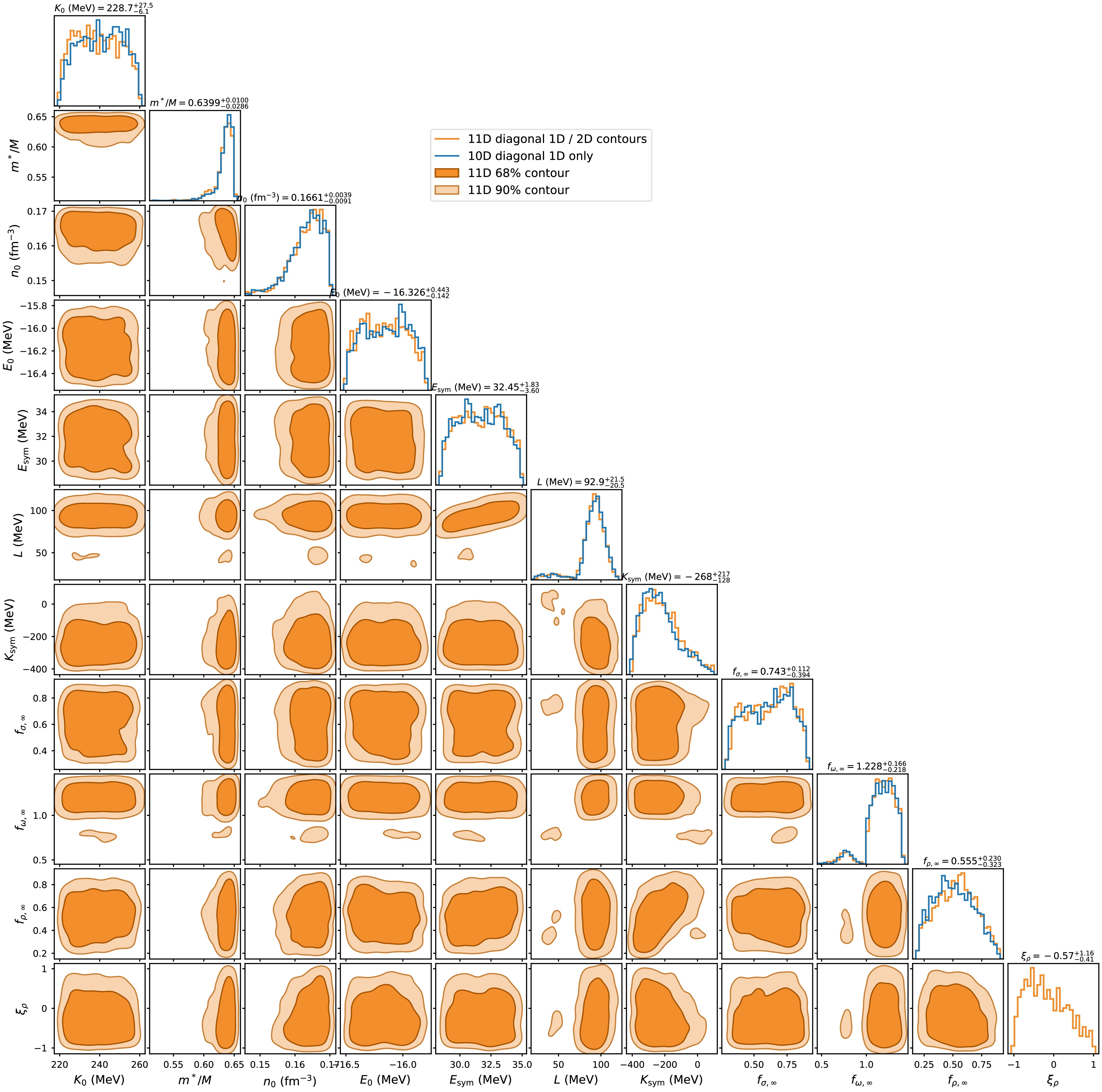
Figure 9. (color online) A corner plot displays the posterior distributions of the 11-dimensional ρ-flex model parameters for the NS+GW data set. Diagonal panels show one-dimensional marginalized posterior distributions; the 10-dimensional baseline posteriors are overlaid for the ten common parameters. Off-diagonal panels show two-dimensional posterior contours for the 11-dimensional model. Diagonal annotations provide the posterior mode and the 90% highest-posterior-density interval.
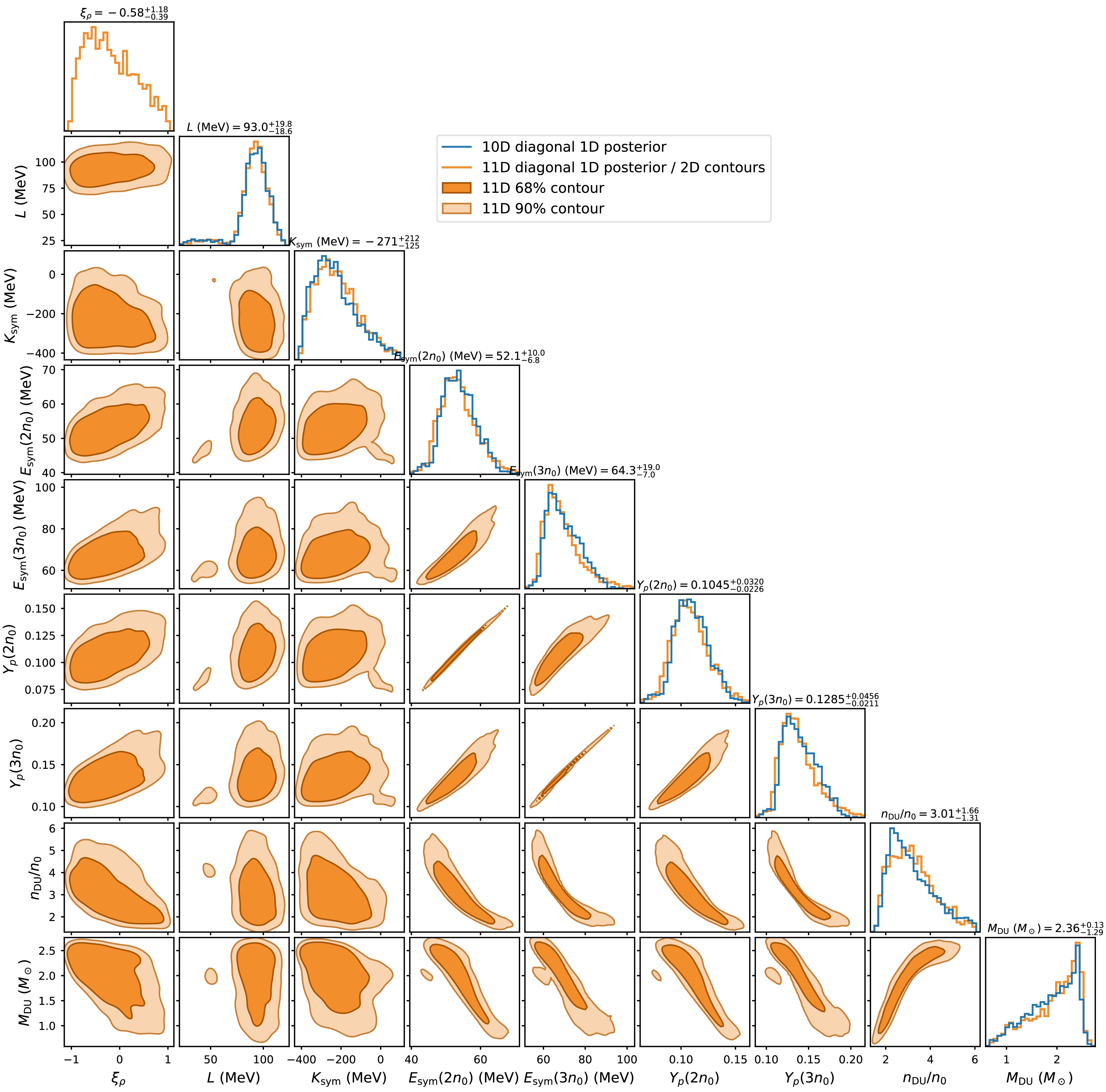
Figure 10. (color online) Corner plot showing selected high-density isovector and direct-Urca observables for the NS+GW data set. The plotted quantities are
$ \xi_\rho $ , L,$ K_{\rm{sym}} $ ,$ E_{\rm{sym}}(2n_0) $ ,$ E_{\rm{sym}}(3n_0) $ ,$ Y_p(2n_0) $ ,$ Y_p(3n_0) $ ,$ n_{\rm{DU}}/n_0 $ , and$ M_{\rm{DU}} $ . Diagonal panels show one-dimensional marginalized posteriors, with the 10D baseline distributions overlaid where applicable. Off-diagonal panels show two-dimensional posterior contours for the 11D model.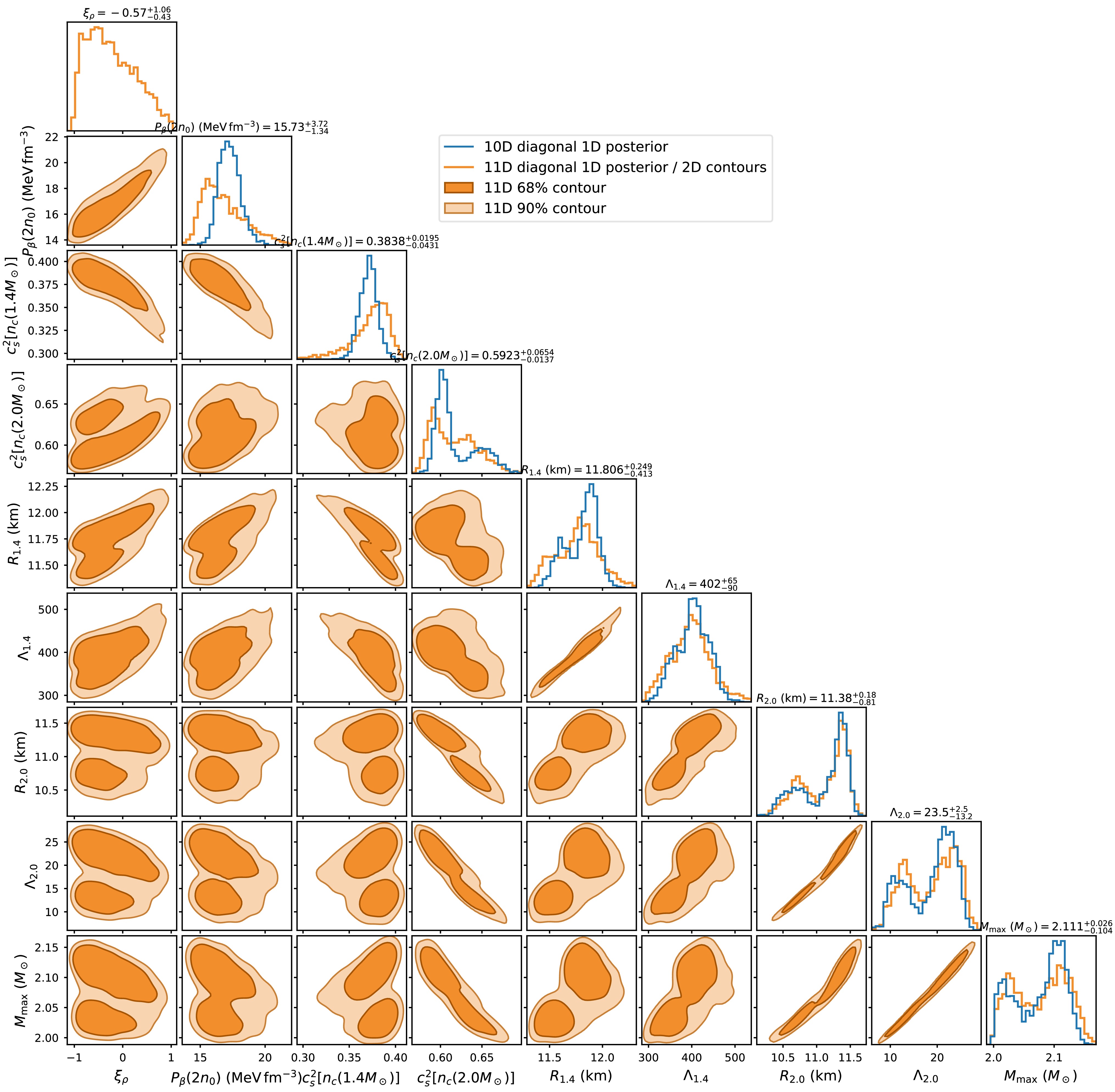
Figure 11. (color online) A corner plot of selected bulk and macroscopic neutron-star observables is shown. The plotted quantities are
$ \xi_\rho $ ,$ P_\beta(2n_0) $ ,$ c_s^2[n_c(1.4M_\odot)] $ ,$ c_s^2[n_c(2.0M_\odot)] $ ,$ R_{1.4} $ ,$ \Lambda_{1.4} $ ,$ R_{2.0} $ ,$ \Lambda_{2.0} $ , and$ M_{\max} $ . The diagonal panels display the one-dimensional marginalized posterior distributions, overlaid with the 10D baseline distributions where applicable. The off-diagonal panels display the two-dimensional posterior contours for the 11D model. -
This appendix presents additional posterior-correlation plots, shown in Figures 9, 10 and 11, which complement the ALL+GW results presented in the main text. The plotting conventions are the same as those used in Figs. 7 and 8. In the diagonal panels, the one-dimensional posterior distributions from the 10D baseline model are overlaid for parameters common to both the 10D and 11D models. The off-diagonal contours show the two-dimensional posterior correlations of the 11D ρ-flex model.
Figure 9. (color online) A corner plot displays the posterior distributions of the 11-dimensional ρ-flex model parameters for the NS+GW data set. Diagonal panels show one-dimensional marginalized posterior distributions; the 10-dimensional baseline posteriors are overlaid for the ten common parameters. Off-diagonal panels show two-dimensional posterior contours for the 11-dimensional model. Diagonal annotations provide the posterior mode and the 90% highest-posterior-density interval.
Figure 10. (color online) Corner plot showing selected high-density isovector and direct-Urca observables for the NS+GW data set. The plotted quantities are
$ \xi_\rho $ , L,$ K_{\rm{sym}} $ ,$ E_{\rm{sym}}(2n_0) $ ,$ E_{\rm{sym}}(3n_0) $ ,$ Y_p(2n_0) $ ,$ Y_p(3n_0) $ ,$ n_{\rm{DU}}/n_0 $ , and$ M_{\rm{DU}} $ . Diagonal panels show one-dimensional marginalized posteriors, with the 10D baseline distributions overlaid where applicable. Off-diagonal panels show two-dimensional posterior contours for the 11D model.
Figure 11. (color online) A corner plot of selected bulk and macroscopic neutron-star observables is shown. The plotted quantities are
$ \xi_\rho $ ,$ P_\beta(2n_0) $ ,$ c_s^2[n_c(1.4M_\odot)] $ ,$ c_s^2[n_c(2.0M_\odot)] $ ,$ R_{1.4} $ ,$ \Lambda_{1.4} $ ,$ R_{2.0} $ ,$ \Lambda_{2.0} $ , and$ M_{\max} $ . The diagonal panels display the one-dimensional marginalized posterior distributions, overlaid with the 10D baseline distributions where applicable. The off-diagonal panels display the two-dimensional posterior contours for the 11D model. -
This appendix presents additional posterior-correlation plots, shown in Figures 9, 10 and 11, which complement the ALL+GW results presented in the main text. The plotting conventions are the same as those used in Figs. 7 and 8. In the diagonal panels, the one-dimensional posterior distributions from the 10D baseline model are overlaid for parameters common to both the 10D and 11D models. The off-diagonal contours show the two-dimensional posterior correlations of the 11D ρ-flex model.
Figure 9. (color online) A corner plot displays the posterior distributions of the 11-dimensional ρ-flex model parameters for the NS+GW data set. Diagonal panels show one-dimensional marginalized posterior distributions; the 10-dimensional baseline posteriors are overlaid for the ten common parameters. Off-diagonal panels show two-dimensional posterior contours for the 11-dimensional model. Diagonal annotations provide the posterior mode and the 90% highest-posterior-density interval.
Figure 10. (color online) Corner plot showing selected high-density isovector and direct-Urca observables for the NS+GW data set. The plotted quantities are
$ \xi_\rho $ , L,$ K_{\rm{sym}} $ ,$ E_{\rm{sym}}(2n_0) $ ,$ E_{\rm{sym}}(3n_0) $ ,$ Y_p(2n_0) $ ,$ Y_p(3n_0) $ ,$ n_{\rm{DU}}/n_0 $ , and$ M_{\rm{DU}} $ . Diagonal panels show one-dimensional marginalized posteriors, with the 10D baseline distributions overlaid where applicable. Off-diagonal panels show two-dimensional posterior contours for the 11D model.
Figure 11. (color online) A corner plot of selected bulk and macroscopic neutron-star observables is shown. The plotted quantities are
$ \xi_\rho $ ,$ P_\beta(2n_0) $ ,$ c_s^2[n_c(1.4M_\odot)] $ ,$ c_s^2[n_c(2.0M_\odot)] $ ,$ R_{1.4} $ ,$ \Lambda_{1.4} $ ,$ R_{2.0} $ ,$ \Lambda_{2.0} $ , and$ M_{\max} $ . The diagonal panels display the one-dimensional marginalized posterior distributions, overlaid with the 10D baseline distributions where applicable. The off-diagonal panels display the two-dimensional posterior contours for the 11D model. -
This appendix presents additional posterior-correlation plots, shown in Figures 9, 10 and 11, which complement the ALL+GW results presented in the main text. The plotting conventions are the same as those used in Figs. 7 and 8. In the diagonal panels, the one-dimensional posterior distributions from the 10D baseline model are overlaid for parameters common to both the 10D and 11D models. The off-diagonal contours show the two-dimensional posterior correlations of the 11D ρ-flex model.
Figure 9. (color online) A corner plot displays the posterior distributions of the 11-dimensional ρ-flex model parameters for the NS+GW data set. Diagonal panels show one-dimensional marginalized posterior distributions; the 10-dimensional baseline posteriors are overlaid for the ten common parameters. Off-diagonal panels show two-dimensional posterior contours for the 11-dimensional model. Diagonal annotations provide the posterior mode and the 90% highest-posterior-density interval.
Figure 10. (color online) Corner plot showing selected high-density isovector and direct-Urca observables for the NS+GW data set. The plotted quantities are
$ \xi_\rho $ , L,$ K_{\rm{sym}} $ ,$ E_{\rm{sym}}(2n_0) $ ,$ E_{\rm{sym}}(3n_0) $ ,$ Y_p(2n_0) $ ,$ Y_p(3n_0) $ ,$ n_{\rm{DU}}/n_0 $ , and$ M_{\rm{DU}} $ . Diagonal panels show one-dimensional marginalized posteriors, with the 10D baseline distributions overlaid where applicable. Off-diagonal panels show two-dimensional posterior contours for the 11D model.
Figure 11. (color online) A corner plot of selected bulk and macroscopic neutron-star observables is shown. The plotted quantities are
$ \xi_\rho $ ,$ P_\beta(2n_0) $ ,$ c_s^2[n_c(1.4M_\odot)] $ ,$ c_s^2[n_c(2.0M_\odot)] $ ,$ R_{1.4} $ ,$ \Lambda_{1.4} $ ,$ R_{2.0} $ ,$ \Lambda_{2.0} $ , and$ M_{\max} $ . The diagonal panels display the one-dimensional marginalized posterior distributions, overlaid with the 10D baseline distributions where applicable. The off-diagonal panels display the two-dimensional posterior contours for the 11D model.
High-density isovector uncertainty and direct-Urca thresholds in a ρ-flex density-dependent relativistic mean-field model
- Received Date: 2026-05-07
- Available Online: 2026-09-15
Abstract: We investigate the role of the model dependence of the high-density isovector sector in neutron-star matter within a density-dependent relativistic mean-field framework. A 10-dimensional TW-like DD-RMF baseline model is compared with an 11-dimensional ρ-flex extension in which an additional parameter, $ \xi_\rho $, introduces a controlled deformation of the high-density ρ-meson channel while leaving the saturation-point isovector properties unchanged. Bayesian inference is performed for two data combinations: NS+GW, which includes neutron-star mass and radius measurements and GW170817 tidal information, and ALL+GW, which further incorporates low-density χEFT and heavy-ion-collision constraints. For each posterior sample, we construct the beta-equilibrated equation of state, solve the stellar structure and tidal-response equations, and determine the direct-Urca threshold. The Bayesian evidence differences, $ \Delta\ln Z_{\rm{INS}}=-0.23\pm0.08 $ for NS+GW and $ -0.02\pm0.17 $ for ALL+GW, indicate that present data do not statistically require the additional ρ-channel flexibility. The 10D and 11D models yield similar posterior predictions for the beta-equilibrium pressure, sound speed, mass-radius relation, tidal deformability, and maximum mass. In contrast, the 11D extension broadens the allowed ranges of the high-density symmetry energy, proton fraction, direct-Urca threshold density, onset mass, and direct-Urca activation probability. These results demonstrate that current multimessenger constraints primarily restrict the bulk stiffness of beta-equilibrated matter, while residual uncertainty in the high-density isovector sector remains relevant for composition-sensitive and cooling-related observables.



 DownLoad: