Probing Quantum Phase Transitions in the sdg-Interacting Boson Model Using von Neumann Entropy

Recently, considerable effort has been devoted to understanding the relationship between entanglement in many-particle systems and QPTs. Quantum phase transitions arise from the constraints imposed by Heisenberg’s uncertainty principle, in clear contrast to classical phase transitions, which are driven solely by thermal fluctuations and occur when a system crosses a critical point defined through macroscopic order parameters [1, 2]. QPTs are generated by changes in an external parameter or coupling constant. These transformations manifest as structural rearrangements in mesoscopic systems, including molecular clusters, semiconductors, atomic nuclei, and even quark matter. They occur at zero temperature and arise solely from quantum fluctuations induced by changes in control parameters. Such quantum phase transitions play a central role across diverse fields, from cosmology to quantum computation and studies of decoherence. Both classical and quantum systems exhibit critical points characterized by a diverging correlation length that governs their behavior near the transition. However, quantum systems exhibit additional correlations that have no classical counterparts [3−5]. This phenomenon, referred to as entanglement [6], serves as a fundamental resource that enables quantum computation and quantum communication [7]. Quantum entanglement is a physical phenomenon that occurs when a group of particles interacts such that the quantum state of each particle cannot be described independently of the states of the others, even when the particles are separated by large distances. The contribution of entanglement to phase transitions cannot be fully described within the framework of conventional statistical mechanics [8]. Quantum entanglement is one of the foundational concepts of quantum physics, first brought into focus through the seminal work of Einstein, Podolsky, and Rosen in 1935 [9]. Quantifying entanglement in multipartite systems remains a challenging problem, and in recent years considerable attention has been directed toward understanding various aspects of entanglement [10−13]. Although the characterization of entanglement in pure states is relatively straightforward, identifying and quantifying entanglement in mixed states remains a complex and largely unresolved mathematical challenge. In recent years, quantum information theory has provided new tools and perspectives for studying entangled nuclear systems, such as atomic nuclei, which inherently behave as multipartite systems [14]. This perspective opens promising possibilities for gaining deeper insight into phenomena governed by the strong interaction [15]. Nuclear many-body systems are self-bound assemblies composed of four types of fermions—protons and neutrons with spin up and spin down—and exhibit a wide range of complex correlation phenomena [16]. If no correlations are present among the nucleons, each particle acts independently, and the nucleus resides in an uncorrelated state. However, describing realistic nuclear systems remains a central challenge in nuclear many-body theory. Consequently, significant efforts are now focused on developing new quantum algorithms capable of addressing the complexities of multi-particle nuclear systems [17−22]. Quantum entanglement is central to virtually all applications of quantum mechanics, which naturally leads to the growing integration of quantum-information concepts and methods into nuclear physics. As a result, both quantum-information researchers and nuclear physicists have become increasingly interested in understanding the entanglement characteristics inherent in nuclear systems and processes [23, 24].

In nuclear physics, quantum phase transitions [25−30] represent sudden structural changes within a nuclear system, affecting both the ground state and the accompanying low-lying excitations. These transitions are most effectively explored through algebraic methods [31], including frameworks such as the $ sd $-IBM [32−36] and its extension, the $ sdg $-IBM [37−46].

In this work, we examine quantum entanglement within the broader context of nuclear structure and quantum information. A principal aim of this study is to characterize quantum phase transitions and nuclear structural evolution through the degree of entanglement. By analyzing how entanglement behaves near quantum critical points, we use it as a diagnostic tool to identify and describe QPTs. The entanglement characteristics of multipartite systems also enable the exploration of various dynamical symmetry limits, offering explicit expressions that can be readily compared with experimental observations.

To probe the phase transition, we compute exact entanglement entropy values across the transitional region of the sdg-IBM, employing the dual algebraic structure of a three-level pairing model formulated within the affine $ SU(1, 1) $ Lie algebra and using Schmidt decomposition techniques. Experimental indications of the $ U_d(5)\otimes U_g(9)\leftrightarrow SO_{sdg}(15) $ transition in even–even nuclei are presented, and the corresponding analysis of the $ {^{108-116}_{48}Cd} $ isotopes is carried out. The von Neumann entropy values for their low-lying states are also reported.

The $ sdg $-IBM, which describes collective excitations in even–even nuclei through nucleon pairs with angular momenta $ L=0 $ (s-boson), $ L=2 $ (d-boson), and $ L=4 $ (g-boson), is described in detail in Refs. [37−48]. In our previous work [49], we proposed an algebraic method based on the dual algebraic structure of a three-level pairing model within the framework of the $ sdg $-IBM for nuclei in the transitional region from the spherical to the γ-unstable quantum shape phase transition. To clarify how possible simplifications provide insight into exactly solvable models, the reader is referred to Refs. [47−53]. In the following sections, we briefly introduce the energy spectrum and von Neumann entropy.

To define the Hamiltonian within the framework of $ sdg $-IBM using the affine $ SU(1,1) $ Lie algebra, the algebraic structure of $ SU(1,1) $ must first be introduced. The $ SU(1,1) $ algebra is generated by $ S^\nu $, with $ \nu =0 $ and $ \pm $, which satisfy the following commutation relations:

The quadratic Casimir operator of $ SU(1,1) $ is given by

The basis states of an irreducible representation (irrep) of $ SU(1,1) $, $ | k\mu\rangle $, are determined by a single parameter, k, which can take any positive value, with $ \mu = k,k+1,\ldots $. Therefore

In the $ sdg $-IBM, the generators of the s-, d-, and g-boson pairing algebras form the $ SU_s(1,1) $, $ SU_d(1,1) $, and $ SU_g(1,1) $ algebras, respectively. They are defined as follows:

In Eq(4), the $ b^{\dagger} $ ($ \widetilde{b} $) and $ n_{b} $ with $ b:=s, d, g $ are the b- boson creation operator (the b- boson annihilation operator) and the number of b- boson operator.

The vector space corresponding to the basis vectors of the s-, d-, and g- bosons is a 15-dimensional vector space. The generators of these bosons in this space form the $ U_{sdg}(15) $ algebra. The subalgebras considered in this study are given as follows:

and

The bases of the $ U_{d}(5)\otimes U_{g}(9)\supset SO_{dg}(14) $ and $ SO_{sdg}(15)\supset SO_{dg}(14) $ subalgebras are simultaneously the bases of $ SU_{d}(1,1)\otimes SU_{g}(1,1)\supset U(1) $ and $ SU_{sdg}(1,1) \supset U(1 $), respectively. The Casimir operators of $ SO_{d}(5)\otimes SO_{g}(9) $ and $ SO_{sdg}(15) $ can be expressed in terms of the Casimir operators of $ SU_{d}(1,1)\otimes SU_{g}(1,1) $, and $ SU_{sdg}(1,1) $ as follows:

Moreover, the infinite-dimensional $ SU(1,1) $ algebra is generated by

where $ c_s $, $ c_{d} $ and $ c_{g} $ are the real parameters and n can be $ 0,\pm1,\pm2,... $. These generators satisfy the commutation relations $ [S^0_m,S^{\pm}_n]=\pm S^{\pm}_ {m+n} $, $ [S^+_m,S^{-}_n]=-2S^0_{m+n+1} $. By employing the generators of algebra $ SU(1,1) $, the proposed Hamiltonian for the transitional region between $ U_{d}(5)\otimes U_{g}(9)\leftrightarrow SO_{sdg}(15) $ (vibrational to γ-unstable transition) limits is

In Eq.(7) α, γ, δ, κ, η, and β are the real parameters. In this equation for $ c_s = c_d = c_g $ describe the $ SO(15)_{sdg} $ limit and also, for $ c_s = 0 $ and $ c_d \neq c_g \neq 0 $ describe the $ U_d(5)\otimes U_g(9) $ limit. Also, the $ c_s \neq c_d\neq c_g \neq 0 $ situation corresponds to $ U_d(5)\otimes U_g(9)\leftrightarrow SO_{sdg}(15) $ transitional region [47−49]. Here, α,γ, δ, κ, η, β are fit parameters and $ c_s $ and $ c_g $ are control parameters. For obtaining the eigenvalues of $ sdg $-Hamiltonian, Eq.(7) the eigenstates are given as

The eigenstates of Eq. (7) can be obtained using the Fourier–Laurent expansion of the eigenstates and $ SU(1,1) $ generators in terms of unknown c-number parameters $ x_i $, with $ i=1,2,\ldots,m $. Thus, the eigenstates can be expressed as follows:

where A is the normalization factor and $ S_{x_i}^{+} $ is

Let $ |lw\rangle $ be the lowest weight state of $ SU(1,1) $, which should satisfy $ S^{-}(s)|lw\rangle=0, S^{-}(d)|lw\rangle=0, S^{-}(g)|lw\rangle=0 $. In the most general form, the $ |lw\rangle $ is given by:

where $ N = \nu_s + \nu_d + \nu_g $, $ n_s = \nu_s $, $ n_d = \nu_d $, $ n_g = \nu_g $. Hence, we have

The eigenvalues $ E^{(m)} $ of the Hamiltonian (7) can be expressed as

Here, $ h^{(m)}=\sum\nolimits_{i=1}^{m}\frac{\alpha}{x_i} $, and the quantum number $ (m) $ is related to the total boson number N by $ N = 2m +\nu_s + \nu_d + \nu_g $. To obtain numerical results for the energy spectra of the nuclei considered, a set of nonlinear Bethe Ansatz equations (BAEs) with m unknowns for m-pair excitations must be solved. The constants in Eq.(13) (γ,δ, κ, η, and β) can also be obtained using the least-squares method (LSM). The set of BAEs using the transformed variables $ C_{s}=\dfrac{c_{s}}{c_{d}}\leq 1, C_{g}=\dfrac{c_{g}}{c_{d}}=1, g=1 , y_{i}={c^{2}_{d}} {x_{i}} $ is given as follows:

Here, $ C_s $ varies between 0 and 1. To calculate the roots of the BAEs for specified values of $ \nu_s $, $ \nu_d $, and $ \nu_g $, we solve Eq. (14) using fixed values of $ C_s $ and α. We then repeat this procedure for different values of $ C_s $ and α to obtain energy spectra that minimize the deviation from the experimental values [54], $ \sigma = (\dfrac{1}{N_{tot}}\sum _{i}^{N_{tot}}|E_{exp}(i)- {E_{cal}(i)|^2})^{\frac{1}{2}} $, where $ N_{tot } $ is the number of energy levels.

We focus on the behavior of the von Neumann entropy in the transitional region and outline the procedure for calculating this quantity in the sdg-IBM. As an appropriate measure of entanglement, the von Neumann entropy provides a straightforward means of quantifying the entanglement between two subsystems. It can be expressed in terms of the singular values obtained from the Schmidt decomposition of the system’s quantum state. In general, any bipartite pure state can be written as [55]:

where $ a_{i} $ is the Schmidt coefficient, and $ |\upsilon_{i} \rangle_{A} $ and $ |\nu_{i} \rangle_{B} $ are orthonormal states in subsystems A and B, respectively. Thus, the von Neumann entropy can be expressed using the Schmidt decomposition as [56−58]

To construct the Von Neumann entropy within the $ sdg $-IBM framework, we treat the s, d and g, sectors as distinct quantum subsystems with corresponding Hilbert spaces $ H_s $, $ H_d $ and $ H_g $. The full Hilbert space of the system is then given by the tensor product $ H=H_{s}\otimes H_{d}\otimes H_{g} $, where each space represents the single-particle states of the s-, d-, and g-bosons. Our goal is to evaluate the Von Neumann entropy associated with these bosonic degrees of freedom. To begin, we define the operators $ S _{x_{i} }^{+} $ as follows:

where $ \alpha_{i}=\dfrac{c_{s}}{1-c_{s}^{2} x_{i} } $, $ \beta_{i}=\dfrac{c_{d}}{1-c_{d}^{2} x_{i} } $, and $ \gamma_{i}=\dfrac{c_{g}}{1-c_{g}^{2} x_{i} } $. We use the following relation [59]:

The Schmidt decomposition in Eq. (15) can be written as:

where the normalization factor (Θ), $ A_{l_1,l_2,l_3} $, and $ b_{l_1,l_2,l_3,k_s,k_d,k_g} $ are defined as follows:

In Eq.(19), the states $ |k_s,k_s+l_1,L,M_L\rangle $, $ |k_d,k_d+l_2,L,M_L\rangle $, and $ |k_g,k_g+l_3,L,M_L\rangle $ correspond to the basis states of the s-, d-, and g-boson subspaces, respectively. In general, the specific choice of basis for each Hilbert space does not affect the entanglement calculation, since any basis can ultimately be transformed into the Schmidt basis. Conveniently, for the bosonic system considered here, the chosen basis already coincides with the Schmidt basis. Consequently, the von Neumann entropy in the $ sdg $-IBM can be written as:

In this calculation, the entanglement between the s boson and the $ dg $ bosons is considered. Therefore, the general form of the wave function is:

where $ |l_1\rangle_s $ are states constructed from s-bosons, and $ |\phi_{l_1}(d,g)\rangle $ are the corresponding states in the $ dg $-sector. The total angular momentum of the s-bosons is zero ($ L=0 $). Therefore, any angular momentum in the full state originates solely from the d- and g-bosons. This is consistent with the structure of the lowest-weight state (Eq. (11)), in which the angular momentum content is carried entirely by the $ dg $-sector. The entanglement discussed in the von Neumann entropy analysis is between subspaces rather than individual particles. The s-boson sector forms collective scalar pairs, since they have $ L=0 $, whereas the $ dg $-boson sector forms collective excitations with angular momentum. Thus, the entanglement between the s-boson sector and the $ dg $-boson sector is indeed between collective modes, such as pairs, condensates, or coherent superpositions, rather than between single s-bosons and individual d or g bosons. $ \phi_{l_1}(d,g) $ and $ {p_{{l_1}}} $ are written as follows:

Finally, the von Neumann entropy (S) is given by

In many transitional nuclei, such as $ Cd $ isotopes near the closed shell $ Z = 50 $, as well as in strongly deformed nuclei, additional experimentally observed low-lying $ 0^+ $, $ 2^+ $, and $ 4^+ $ states cannot be explained within the $ (sd)^N $ boson space. Other experimental evidence, such as the $ k^{\pi} = 0^+_3, 3^+_1, 2^+_2 $, and $ 4^+ $ bands, can be interpreted as bands built on hexadecupole vibrations and hexadecupole transition densities associated with the excitation of some $ 4^+ $ levels in $ Cd $ isotopes. Moreover, the $ sd $-IBM is designed for low-lying states, usually with energies below 2.5 $ MeV $. By introducing the g-boson, the investigation of higher-lying states becomes possible. For example, higher states such as $ 0^+_4 $, $ 2^+_4 $, $ 4^+_3 $ (g-boson state), $ 4^+_4 $,.... are investigated, and good results are obtained.

The fit parameters for the energy spectra of selected Cadmium isotopes ($ {^{108-116}_{48}Cd} $), along with their standard deviations (σ), are listed in Table 1. The small values of σ indicate good agreement between the experimental spectra and those predicted by the $ sdg $-IBM. The experimental and theoretical energies of the investigated levels of the $ {^{108-116}_{48}Cd} $ isotopes, together with the quantum labels for each level, are presented in Tables 2a to 2e. The corresponding experimental and theoretical energy spectra are also shown in Figure 1. At first glance, the close similarity between the experimental and theoretical spectra indicates the accuracy and efficiency of the $ sdg $-IBM. More quantitatively, the standard deviation values confirm this conclusion. Using energy ratios such as ($ {R_{{4 / 2}}} = {{E\left( {4_{_1}^ + } \right)} / {E\left( {2_{_1}^ + } \right)}}\ $) and ($ {R_{{0 / 2}}} = {{E\left( {0_{_1}^ + } \right)} / {E\left( {2_{_1}^ + } \right)}}\ $), one can make predictions about the shape-phase transition from spherical to γ-unstable nuclei. For example, $ 2.2 \leqslant{R_{{4 / 2}}} \leqslant 2.5\ $ characterises the spectrum of transitional nuclei in the spherical to γ-unstable region. These energy ratios have been obtained within the framework of the $ sdg $-IBM for $ {^{108-116}_{48}Cd} $ and compared with experimental data. The results are shown in Figure 2. The calculated values of $ 2.29 \leqslant R_{{4 / 2}}^{cal} \leqslant 2.65 $ for this chain confirm the transition region from spherical to γ-unstable.

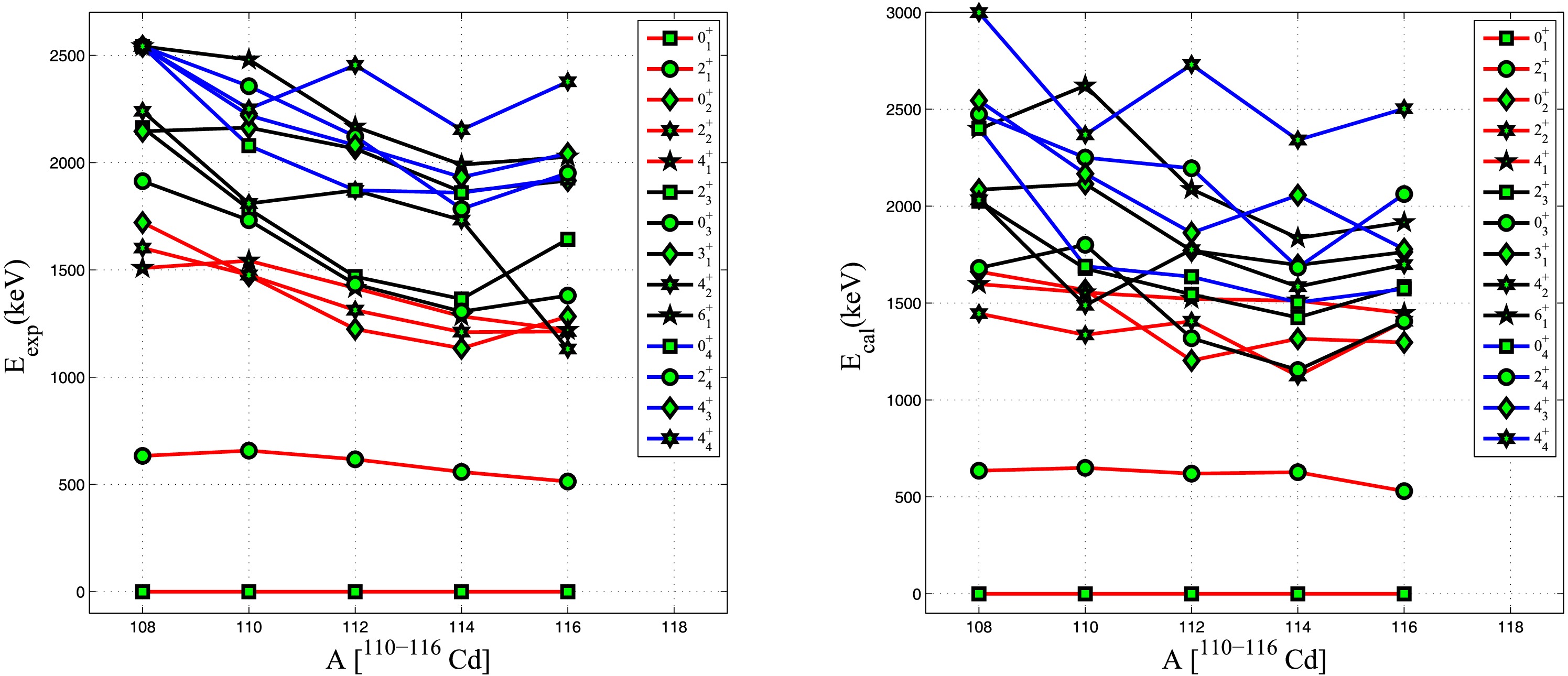
Figure 1.  (color online) Comparison of experimental and calculated energies for the $ Cd $ isotope.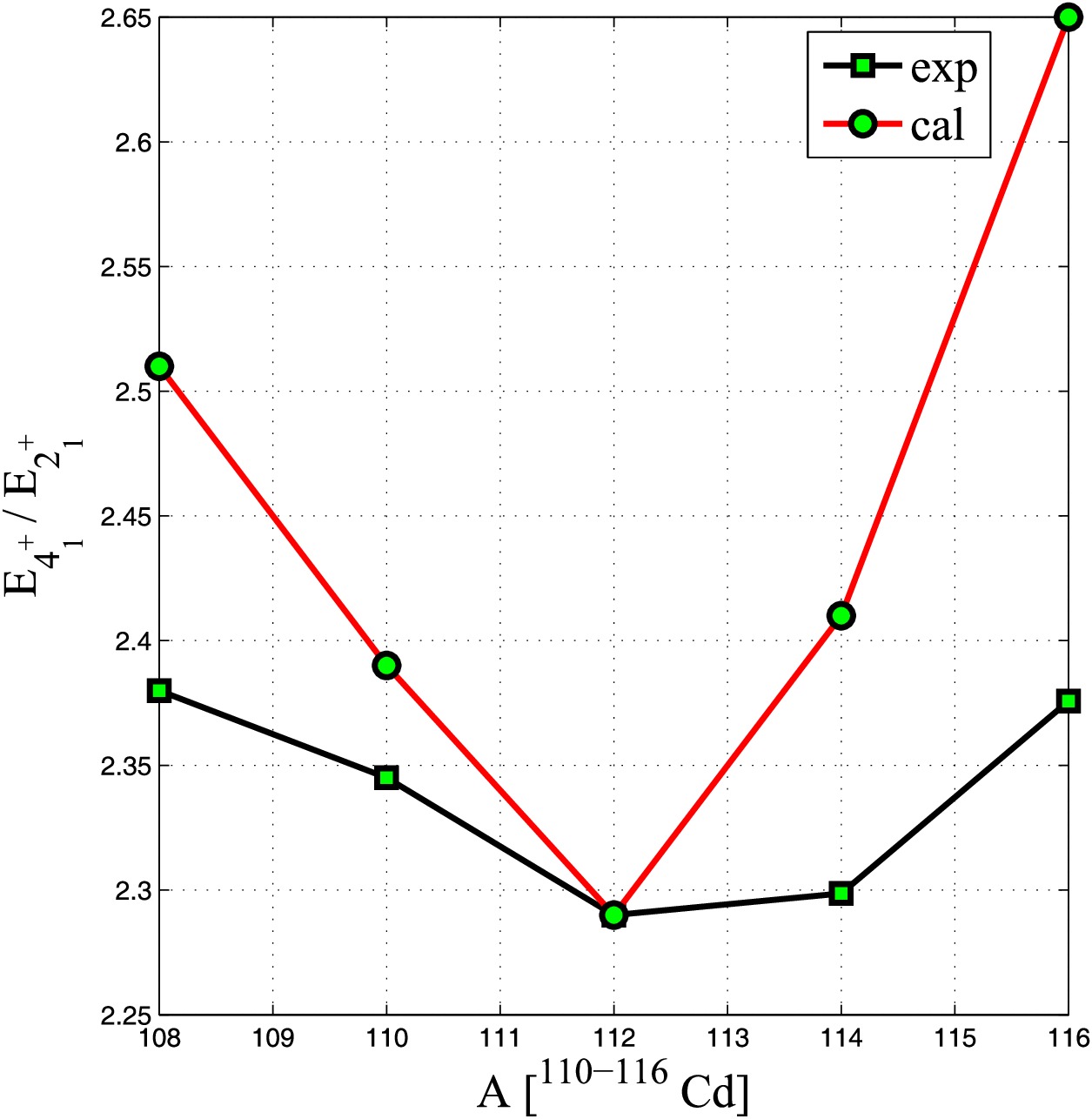

Figure 2.  (color online) Comparison of theoretical and experimental values of $ R_{4/2}=\frac{E(4_1^+)}{E(2_1^+)} $ and $ R_{0/2}=\frac{E(0_2^+)}{E(2_1^+)} $ for Cd isotopes.

Next, we compare these results with the von Neumann entropy. As explained in Sec. 2.2, the signature of the phase transition in even-even nuclei can be identified using the von Neumann entropy. Here, the von Neumann entropy is used to investigate the transition from spherical ($ U_d(5)\otimes U_g(9) $) to γ-unstable ($ SO(15) $) limits in even-even nuclei. We have calculated the von Neumann entropy within the $ sdg $-IBM framework using the dual algebraic structure based on the affine $ SU(1,1) $ Lie algebra and the Schmidt decomposition. The spherical limit occurs for $ C_s = \dfrac{c_s }{c_d}= 0 $, $ c_d = 1 $, $ c_g = 1 $, and the γ-unstable limit occurs for $ C_s = \dfrac{c_s}{c_d}= 1 $, $ c_s = c_d = c_g = 1 $. Theoretically, the von Neumann entropy as a function of the control parameter $ C_s $ has been calculated for each state. It shows how the von Neumann entropy of the s- and $ dg $-boson sectors changes from $ U_d(5)\otimes U_g(9) $ to $ SO(15) $.

To analyse QPT, the von Neumann entropy for the $ {^{108-116}_{48}Cd} $ isotopes has been calculated. Using this observable, we examine whether these nuclei exhibit transitional behavior indicative of shapes intermediate between the spherical and γ-unstable limits. Studies have shown that these isotopes have $ U_d(5)\otimes U_g(9)\leftrightarrow SO(15) $ transitional characteristics. The optimal sets of transitional Hamiltonian parameters have been obtained using the LSM. The experimental data for the $ {^{108-116}_{48}Cd} $ nuclei are taken from Refs. [54]. The computed von Neumann entropies for the low-lying states of the $ {^{108-116}_{48}Cd} $ isotopes, along with the predicted values for both low- and high-spin states, are shown in Fig. 3. The behavior of the control parameter $ C_s $ indicates structural evolution and shape-phase transitions across the Cd isotopic chain. According to Fig. 3 and Tables 2.a-2.e, the von Neumann entropy of the s- and $ dg $-boson sectors is zero for vibrational nuclei and increases with increasing isotope mass. As shown in Tables 2.a-2.e, the control parameter $ C_s $ increases from 0.26 in $ {^{108}_{48}Cd} $ to 0.64 in $ {^{116}_{48}Cd} $, indicating a transition from spherical to γ-unstable structure.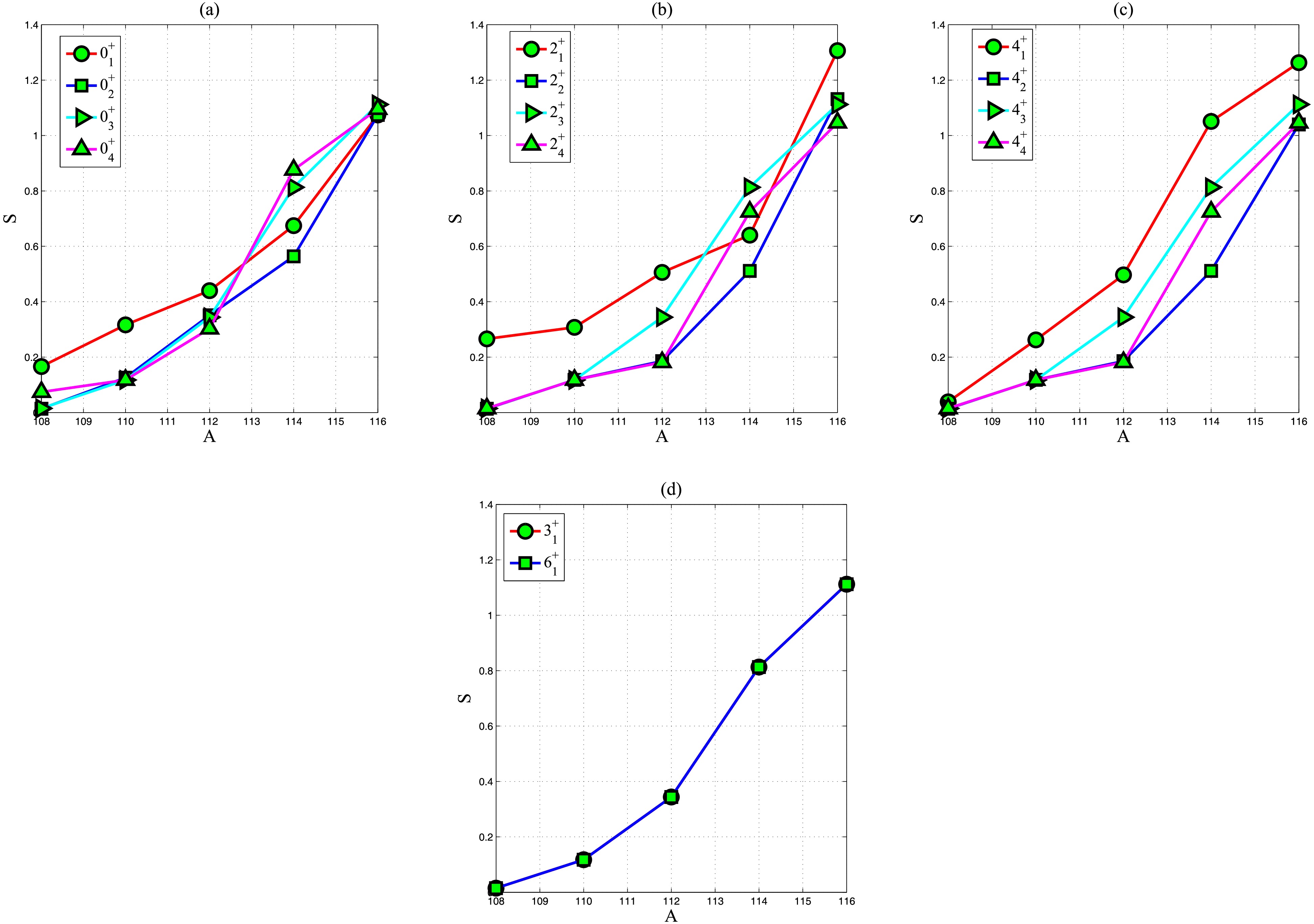

Figure 3.  (color online) Calculated entropies for all low and high states and for selected states of $ Cd $ isotopes.

In this study, we examined the von Neumann entropy as an observable for investigating QPTs. Our analysis focused on the $ sdg $-IBM, a three-level pairing scheme that effectively represents a qubit-like interacting structure. We introduced a procedure for evaluating the von Neumann entropy in interacting nuclear systems and demonstrated that this quantity serves as an effective order parameter for identifying shape-phase transitions in nuclei. The von Neumann entropies were computed and analyzed for the low-lying states of the $ {^{108-116}_{48}Cd} $ isotopes. The results show that, in the $ U_d(5)\otimes U_g(9) $ limit, the s- and $ dg $-bosons are not entangled, whereas the $ SO(15) $ limit corresponds to maximal entanglement. These findings confirm that the von Neumann entropy is a reliable and meaningful signature for characterizing shape-phase transitions in nuclei.