Acoustic Black Hole in Hayward Spacetime: Shadow, Quasinormal Modes and Analogue Hawking Radiation

Black holes, among the most important predictions of general relativity, occupy a crucial role in classical gravity, semiclassical gravity, and quantum gravity. Their existence has been confirmed through two landmark observational breakthroughs. First, the LIGO and Virgo Collaboration detected the gravitational-wave signal GW150914 from a binary black hole merger [1]. Subsequently, the Event Horizon Telescope (EHT) obtained direct images of supermassive black hole shadows, first at the center of the galaxy M87 (M87*) [2] and later at the center of our own Milky Way, Sagittarius A* [3]. Together, these observations provide complementary and conclusive evidence for the physical reality of black holes in our universe. Beyond these observational confirmations, black holes are theoretically predicted to exhibit other fundamental properties, such as quasinormal modes (QNMs) [4, 5] and Hawking radiation [6, 7]. Among these, Hawking radiation has not yet been observed because of its relatively weak energy scale and the limited sensitivity of current instruments.

In order to detect these phenomena in the laboratory, alternative approaches have been proposed, such as probing Hawking-like radiation in acoustic black holes from analogue gravity [8]. For example, sound-mode perturbations in a fluid within flat spacetime can be described by a scalar field propagating in an effective curved metric, where different velocity profiles of the flow correspond to distinct analogue metrics, thereby enabling the construction of acoustic black holes [9]. Theoretically, the properties of acoustic black holes, including their horizons, ergospheres, analogue Hawking radiation, and tidal deformations, have been extensively examined [10–14]. The stability of such systems has also been studied through analyses of QNMs [15, 16]. See [17–20] for additional references on acoustic analogues of the expanding universe in the Bose-Einstein condensate (BEC). Experimentally, a sonic black hole in a BEC has been realized in [21], followed by observations of analogue Hawking radiation and its corresponding Hawking temperature [22, 23]. Moreover, progress on simulated Hawking emission has been made in optical platforms [24, 25]. A comprehensive overview of both theoretical insights and experimental advances in this field has been provided in the review [8].

On the other hand, analogue gravitational systems not only exist in flat spacetimes, but their typical features can also appear in curved spacetimes. For example, acoustic black hole geometries can be derived from relativistic Gross-Pitaevskii (GP) theory and Yang-Mills (YM) theory in real black hole spacetime backgrounds [26]. Recent works have constructed acoustic black holes within Schwarzschild and charged black hole backgrounds, analyzing various interesting properties, including quasi-bound states [27, 28], QNMs, Hawking radiation, and black hole shadows [29, 30]. The orbits of test vortices and sound waves in an acoustic black hole from relativistic GP theory have also been studied in three-dimensional curved spacetime [31]. Moreover, the information paradox of an acoustic black hole in Schwarzschild spacetime has been investigated using the island formula [32]. Astrophysical black holes are typically surrounded by accretion disks composed of plasma [33], or are embedded in environments such as the cosmic microwave background radiation or superfluids. These environments can be described by relativistic fluid dynamics, thereby providing favorable conditions for the formation of acoustic black holes. Investigating acoustic black holes within astrophysical black hole backgrounds not only enhances our understanding of sound-wave propagation near these celestial objects, which may help extract useful information about the background black hole, but also broadens the scope of analogue gravity.

Previous studies of acoustic black holes in curved spacetimes remain confined to singular background spacetimes. It is therefore of interest to extend such studies to regular black hole backgrounds, which refer to a class of black hole solutions that possess event horizons but are free of essential singularities throughout the entire spacetime [34–36]. These solutions can be constructed from models within nonlinear electrodynamics [37, 38], modified gravity theories [39], and the mechanism of atemporality [40, 41]. Many important properties of regular black holes have been extensively studied, such as particle geodesics [42, 43], shadows [44, 45], QNMs [46–49], and thermodynamic behaviors [50]. Moreover, the microlensing of regular black holes has been investigated via ray-tracing methods [51]. Studying acoustic black holes within a regular black hole spacetime can help us examine the influence of singularities in background black holes, which provides potential applications in distinguishing regular black holes from black holes with singularities. In addition, it provides a useful framework for analyzing sound-wave propagation in the vicinity of regular black holes.

In the present paper, we aim to investigate the near-horizon properties associated with observable quantities of acoustic black holes within the Hayward black hole background [34], which is a typical class of regular black holes that has attracted much attention recently. In other words, we investigate the so-called acoustic Hayward black hole, focusing on the acoustic shadow, QNMs, grey-body factors, and the energy emission rate of analogue Hawking radiation for this system. The acoustic shadow can be studied through phonon propagation, which is effectively described by null geodesics in the analogue gravity framework. Meanwhile, QNMs and analogue Hawking radiation can be analyzed via scalar fields within the same analogue gravity formalism. Explicitly, by examining the critical null geodesics, the shadow of the acoustic horizon is sketched. Then, the QNM frequencies of the acoustic Hayward black hole are computed numerically using the WKB method, confirming the stability of the system, and variations in the QNM frequencies are shown to correlate with the behavior of the effective potential. Moreover, the WKB method is also employed to calculate the grey-body factor and energy emission rate of the analogue Hawking radiation. Our results show that, as the tuning parameter increases, the grey-body factor, the energy emission rate, and the shadow radius all increase significantly. In contrast, the absolute values of the QNM frequencies decrease accordingly, and the potential function becomes smoother, indicating that the QNMs tend to stabilize in the acoustic scenario. Furthermore, as the Hayward parameter increases, the acoustic shadow slightly diminishes, and the analogue Hawking radiation also weakens slightly. Our results not only extend studies of acoustic black holes to regular black hole spacetimes, but may also be useful for future experimental tests of astrophysical black holes.

This paper is organized as follows: In Sec. II, we construct the metric of the acoustic Hayward black hole and analyze its horizon structure. After a brief review of the horizon structure of the Hayward black hole, we recall the formulation of analogue gravity within the GP theory and apply it to the Hayward spacetime background. In Sec. III, the acoustic shadow of the acoustic Hayward black hole is examined by analyzing null geodesics. The variation of the shadow radius with different parameters is discussed. Subsequently, in Sec. IV, we analyze the covariant scalar field equation and the effective potential in acoustic Hayward spacetime, laying the groundwork for subsequent calculations. In Sec. V, the WKB method is employed to numerically compute QNMs for various parameter choices, and the stability of the acoustic Hayward black hole is examined. We also verify the relationship between QNMs and the acoustic sphere (and the acoustic shadow) in the eikonal limit. Then, in Sec. VI, the grey-body factors and energy emission rates in analogue Hawking radiation are calculated, also using the WKB method. Finally, Sec. VII presents the conclusions and discussions.

The Hayward black hole is a typical example of a regular black hole that can be constructed via nonlinear electrodynamics. The action for an electrically charged black hole is given by [38]

Here, we have defined $ \mathfrak F \equiv F_{\mu\nu} F^{\mu\nu} $, where $ F= \mathrm d A $ is the field strength of the electromagnetic field associated with the vector potential $ A^\mu $, and $ \mathcal{L}(\mathfrak{F}) $ is the electromagnetic Lagrangian density. According to the principle of least action, the gravitational field equations are

where $ G_{\mu\nu}=R_{\mu\nu}-\frac{1}{2}Rg_{\mu\nu} $ is the Einstein tensor, and the stress tensor is

where $ \mathcal{L}_{\mathfrak{F}}:=\dfrac{\partial\mathcal{L}}{\partial \mathfrak{F}} $. The equations of motion for the electromagnetic field are

combined with the Bianchi identities

The electromagnetic field can be fully determined, where $ \star $ denotes the Hodge dual. Therefore, in nonlinear electrodynamics, different electromagnetic Lagrangians $ \mathcal{L}(\mathfrak{F}) $ lead to distinct spacetimes and electromagnetic fields [38, 52]. In particular, the Hayward black hole can be constructed as a purely magnetically charged black hole with Lagrangian density [38]

where the Hayward parameter $ L>0 $ is a length-scale parameter [36] related to the magnetic charge $ q_m $ of the Hayward black hole through $ q_m=\dfrac{1}{2}\sqrt[3]{r_s^2L} $, with $ r_s=2M $ denoting the Schwarzschild radius [38]. Consequently, the Hayward metric is given by

with the lapse function as given in [34]

For the subsequent discussion, we define $ g(r):=\dfrac{r_s r^2}{r^3+r_s L^2} $. This Hayward black hole indeed avoids the intrinsic singularity at its center, since as $ r\rightarrow0 $, the lapse function behaves as $ f(r)\rightarrow1-\dfrac{r^2}{L^2} $, exhibiting the form of a de Sitter spacetime core with finite curvature. At spatial infinity, as $ r\rightarrow \infty $, $ f(r)\rightarrow 1-\dfrac{r_s}{r} $, matching the asymptotic form of the Schwarzschild spacetime.

To analyze the horizon structure of the Hayward black hole, we rewrite the lapse function $ f(r) $ in polynomial form: [50]

where

which is an ordinary cubic polynomial. To find its roots, a standard technique is to shift the variable r via $ r=x+\dfrac{r_s}{3} $, which transforms $ P_3 $ into a polynomial in x with the quadratic term absent:

where the coefficients $ g_2 $ and $ g_3 $ are given by

with the constant $ L_0 $ defined as

According to [53], the discriminant of the cubic polynomial in Eq. (11) is given by

and the sign of the discriminant $ \Delta_c $ determines the nature of the roots as follows [50]:

● For $ \Delta_c>0\ (L<\sqrt{2}L_0) $, there are three distinct real roots: two positive and one negative;

● For $ \Delta_c=0\ (L=0, \sqrt{2}L_0) $, there is one positive double root and one distinct negative root;

● For $ \Delta_c<0\ (L>\sqrt{2}L_0) $, there is one negative root and a pair of complex conjugate roots.

Therefore, a Hayward black hole possesses an event horizon only if $ \Delta_c\geq0 $, that is, $ 0\leqslant L\leqslant \sqrt{2}L_0 $. The horizon radius is determined by solving the equation

Using the substitution $ x=\sqrt{\dfrac{g_2}{3}}\cos\alpha $, the equation simplifies to

Using the trigonometric identity

we further obtain

For $ \Delta_c\geq0 $, we have $ -1\leqslant 1-\dfrac{L^2}{L_0^2}\leqslant 1 $, ensuring that α is real. The general solution can be written as

The outermost root, which corresponds to the event horizon, is obtained for $ n=0 $, yielding

Finally, transforming back to the original variable, the event horizon radius of the Hayward black hole is

Returning to the construction of the acoustic black hole in relativistic GP theory [26], we consider fluctuations of a complex scalar field φ. The action of GP theory is given by [54, 55]

where b is a constant and $ m^2 $ is a temperature-dependent parameter that governs the behavior of the system near the critical temperature $ T_c $, scaling as $ m^2\sim (T-T_c) $. In a static background spacetime with metric

The equation of motion for φ follows as

where $ \square\varphi:=\dfrac{1}{\sqrt{-g}}\partial_\mu\left(\sqrt{-g}g^{\mu\nu}\partial_\nu\varphi\right) $. Using the Madelung representation $ \varphi=\sqrt{\rho({x\mathit{\boldsymbol{}}},t)}e^{i\theta({x\mathit{\boldsymbol{}}},t)} $, the complex field φ can be separated, and the equation of motion (24) decomposes into its real and imaginary parts. The real component yields the Euler equation

where the first term corresponds to the quantum potential, $ \dfrac{\square\sqrt\rho}{\sqrt\rho} $. In the long-wavelength approximation adopted here, this quantum potential term is neglected [26]. Meanwhile, the imaginary part takes the form

which simplifies to the continuity equation.

Consider small fluctuations $ (\rho_1,\theta_1) $ about a background configuration $ (\rho_0,\theta_0) $, i.e., $ \rho=\rho_0+\rho_1 $ and $ \theta=\theta_0+\theta_1 $. Linearizing Eqs. (25) and (27) yields, at leading order,

where $ v_\mu $ is defined by $ v_t:=-\partial_t\theta_0 $ and $ v_i:=\partial_i\theta_0 $. At subleading order, we obtain

which is a relativistic d'Alembertian equation for the phase fluctuation $ \theta_1 $ (i.e., the phonon) propagating in an effective curved spacetime described by the effective metric $ \mathcal{G}_{\mu\nu} $, which is

with $ c_s^2:=\dfrac{1}{2}b\rho_0 $. It is evident that the effective metric $ \mathcal{G}_{\mu\nu} $ depends on both the background spacetime $ \mathrm d s^2_{\text{bg}} $ and the fluid four-velocity $ v_\mu $. When the four-velocity has only nonzero t and r components, namely, $ v_t\neq0 $, $ v_r\neq0 $, and $ v_\theta=v_\phi=0 $, the effective metric can be further reduced to [26]:

To proceed, we diagonalize the effective metric using the coordinate transformation $ (\mathrm d t-\dfrac{v_tv_r}{c_s^2-v_rv^r} \mathrm d r)\rightarrow \mathrm d t $. Imposing the condition $ g_{tt}g_{rr}=-1 $ on the background spacetime, the effective line element becomes

Thus, the analogue gravitational metric emerging from the relativistic GP theory is derived.

We now embed the effective metric in Eq. (32) into the Hayward background spacetime described by Eq. (7). This corresponds to studying the acoustic black hole arising in a fluid governed by GP theory in the vicinity of a Hayward black hole. In other words, we construct the acoustic Hayward black hole. To determine the effective metric in analogue gravity, the four-velocity of the fluid must be specified. In this paper, we consider a fluid that starts at rest at infinity and undergoes radial free fall outside a Hayward black hole. Thus, the radial component $ v_r $ corresponds to the escape velocity from a given radius r, and is given by $ v_r=\sqrt{g(r)\xi} $, where $ \xi>0 $ acts as a tuning parameter whose range for the existence of an acoustic horizon will be discussed later. Upon rescaling $ m^2\rightarrow \dfrac{m^2}{2c_s^2} $ and $ v_\mu v^\mu\rightarrow \dfrac{v_\mu v^\mu}{2c_s^2} $, the relation $ v_\mu v^\mu=m^2-1 $ is obtained. At the critical temperature of GP theory, where $ m^2 $ vanishes, it follows that $ v_\mu v^\mu=-1 $. Setting $ c_s=\dfrac{1}{\sqrt{3}} $ for convenience and substituting the four-velocity and the Hayward background spacetime (7) into the effective line element (32), we obtain the line element of the acoustic Hayward black hole as

where

Using the definition of $ g(r) $ given in Eq.(8), this can be written more compactly as

We can see that the acoustic Hayward black hole described by Eq. (33) reduces to the original Hayward black hole, Eq. (7), in the limit $ \xi\rightarrow 0 $. Conversely, as $ \xi\rightarrow \infty $, the acoustic Hayward black hole fills the entire spacetime, as will be examined in more detail in the subsequent discussion.

The acoustic horizon is determined by solving $ \mathcal{F}(r)=0 $. The vanishing of the first term in Eq. (35) gives the horizon of the background Hayward black hole, Eq. (21), while setting the second term to zero gives the acoustic horizon of the acoustic Hayward black hole, which satisfies

This can be simplified to

We define $ \dfrac{1}{2}\pm\sqrt{\dfrac{1}{4}-\dfrac{1}{\xi}}:=\lambda_\pm $. This result also imposes the constraint $ \xi\geq4 $ for the existence of an acoustic black hole. Substituting the expression for $ g(r) $ defined in Eq. (8) into Eq. (37), we obtain the following cubic equation for the acoustic horizon radius r:

which has a form similar to that of the Hayward horizon equation (10). Therefore, we can apply the same method, making the substitution $ r=x+{\frac{r_s}{3\lambda_\pm}} $ to eliminate the quadratic term. After this transformation, Eq. (38) becomes

where the coefficients $ \tilde{g}_2 $ and $ \tilde{g}_3 $ are defined as follows:

and $ \tilde{L}_\pm=\sqrt{\dfrac{2}{27\lambda^3_\pm}}r_s $. Similarly, the discriminant of the cubic equation is

The acoustic horizon exists only when $ 0\leqslant L\leqslant \sqrt{2}\tilde L_\pm $, which ensures that the discriminant satisfies $ \tilde\Delta_c\geq0 $. Following the same procedure as in Eq. (16) to Eq. (19), the solutions for x are given by

Finally, the acoustic Hayward horizons are obtained as

Given that $ 0<\lambda_-\leqslant \dfrac{1}{2}\leqslant \lambda_+<1 $, we have $ r_+'\geq r_-' $, with equality holding at $ \xi=4 $, corresponding to the extremal acoustic Hayward black hole. Moreover, when the Hayward black hole and the acoustic black hole are considered simultaneously, the conditions $ \Delta_c\geq0 $ and $ \tilde\Delta_c\geq0 $ imply $ 0\leqslant L\leqslant \sqrt{2}L_0 $. To compare the relative sizes of $ r_{\text H} $ and $ r_\pm' $, note that the relation $ -1<1-\dfrac{L^2}{L_0^2}<1-\dfrac{L^2}{(\tilde L_\pm)^2}<1 $ gives $ \cos\alpha<\cos\tilde\alpha_\pm $, which guarantees that the acoustic horizons $ r_\pm' $ always lie outside the Hayward horizon $ r_\text H $, as expected. In summary, we find that

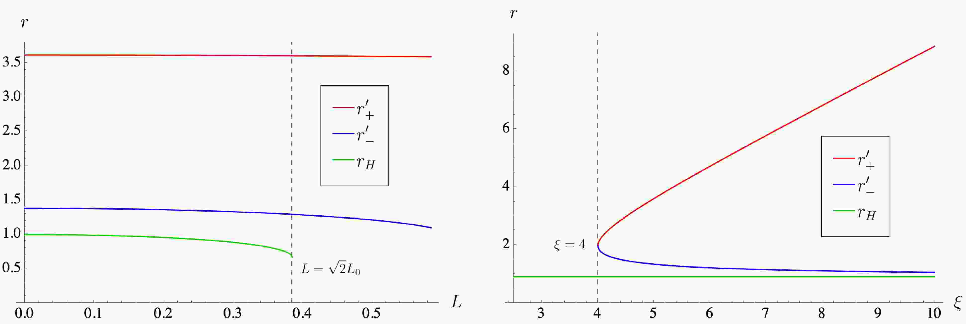
The Hayward horizon and acoustic horizons are illustrated in Fig. 1. Without loss of generality, we set $ r_s=1 $ in the following discussion. In the left panel, with $ \xi=5 $ fixed, we show how the horizon radii vary with the Hayward parameter L. One can see that $ r_+'>r'_->r_{\text H} $ and that the Hayward black hole exists for $ 0\leqslant L\leqslant \sqrt{2}L_0 $. In the right panel, with $ L=L_0 $ fixed, we plot the horizon radii as functions of the tuning parameter ξ. The acoustic horizons $ r_\pm' $ exist for $ \xi\geq4 $, and the case $ \xi=4 $ corresponds to the extremal acoustic black hole, as noted earlier. In the limit $ \xi\rightarrow \infty $, we have $ r'_+\rightarrow \infty $, indicating that sound cannot escape from the entire spacetime, which is consistent with the preceding discussion. In summary, for $ \xi\geq 4 $ and $ 0\leqslant L\leqslant \sqrt{2}L_0 $, the analogue metric embedded in the Hayward spacetime partitions the spacetime into four regions:

Figure 1.  (color online) Horizon structure of the acoustic Hayward black hole. Left panel: radii of the outer acoustic horizon $ r_+' $, inner acoustic horizon $ r_-' $, and Hayward horizon $ r_{\text H} $ as functions of L at fixed $ \xi=5 $. The vertical dashed line indicates the critical value $ L=\sqrt{2}L_0 $. Right panel: the same horizon radii as functions of ξ at fixed $ L=L_0 $. The vertical dashed line marks the critical value $ \xi=4 $.

● $ r<r_{\text H} $: the interior of the Hayward black hole;

● $ r_{\text H}<r<r_-' $: a region from which light can escape and sound can also escape, but sound cannot be detected by an observer outside this region;

● $ r_-'<r<r_+' $: a region from which light can escape but sound cannot;

● $ r>r_+' $: a region from which both light and sound can escape.

In the subsequent analysis, the acoustic horizon is identified as the outer horizon $ r_+' $.

We begin by investigating the acoustic shadow of the acoustic Hayward black hole. In analogue gravity, sound rays follow the null geodesics of the acoustic metric [8]. Consequently, an acoustic black hole also exhibits an acoustic shadow for a distant observer. The formation of such a shadow can be understood with the aid of Fig. 2. The grey region represents the acoustic black hole, and the rightmost point corresponds to the observer. The observation of the acoustic black hole by the observer can be described in terms of null geodesics. As illustrated, these null geodesics fall into two categories: those shown in blue and those in green. The blue geodesics are ultimately captured by the acoustic black hole, whereas the green ones, though deflected, manage to escape. The boundary between captured and escaping trajectories is defined by the red geodesics, which play a pivotal role in the formation of the acoustic shadow. In what follows, we therefore concentrate our analysis on this particular class of critical null geodesics.

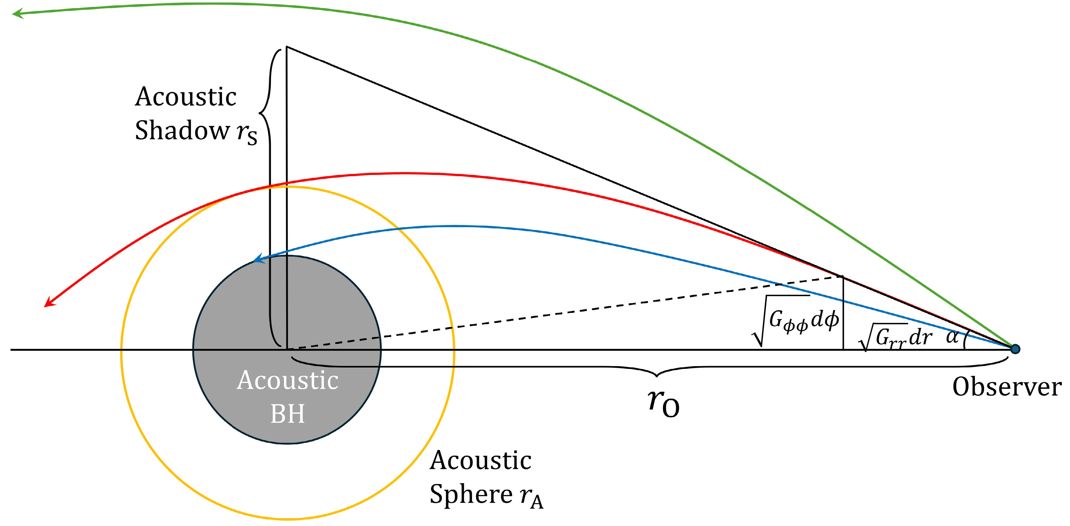
Figure 2.  (color online) Schematic of the acoustic black hole shadow. The central gray circle denotes the acoustic black hole, which is surrounded by an acoustic sphere (yellow circle) of radius $ r_\text A $. Null geodesics emitted from the observer on the right are grouped into three families: blue trajectories captured by the acoustic black hole, green trajectories that escape after deflection, and red critical geodesics that determine the acoustic shadow between the captured and escaping paths.

For geodesics, the Lagrangian takes the following form:

The equations of motion are obtained from

Along null geodesics, the following condition is satisfied:

We consider null geodesics in the equatorial plane, i.e., $ \theta=\dfrac{\pi}{2} $.

The observer perceives the surrounding space as Euclidean [56]; thus, the shadow radius corresponds to $ r_{\text{S}} $, as determined by the tangent to the red geodesic, as shown in Fig. 2. Moreover, the relation between $ r_{\text{S}} $ and $ r_{\text{O}} $ is

where $ \dfrac{ \mathrm d \phi}{ \mathrm d r} $ can be obtained from Eq. (47).

where $ \dot t $ and $ \dot\phi $ are determined by the t and ϕ components of the Lagrange equations (46), respectively. These quantities are related to two constants of motion along the red geodesic, expressed as

Hence, $ \dfrac{ \mathrm d \phi}{ \mathrm d r} $ can be expressed in terms of E and L as

Substitution of this result into Eq. (48) yields

where $ \dfrac{E}{L} $ is fixed by an additional property of the critical red geodesic: for such an orbit, the minimum distance from the acoustic black hole should equal the radius of the acoustic sphere, $ r_\text{A} $, as shown in Fig. 2, which depicts the circular null geodesics around the acoustic black hole [56]. This condition implies

where $ r_{\text{A}} $ denotes the radius of the acoustic sphere. Then, substituting

into Eq. (52) gives

For an observer at infinity, $ r_{\text{O}}\rightarrow \infty $, and $ \mathcal{F}(r_{\text{O}})\rightarrow1 $. As a result,

The final quantity to determine is the radius of the acoustic sphere, $ r_{\text{A}} $. This can be obtained by evaluating $ \dfrac{ \mathrm d^2 r}{ \mathrm d\phi^2} $ on the acoustic sphere, which is done by differentiating $ \dfrac{ \mathrm d r}{ \mathrm d\phi} $. On the acoustic sphere, r is constant, so this second derivative must vanish, i.e.,

where E and L also clearly satisfy Eq. (53), and $ \mathcal{F}^\prime(r)=\dfrac{ \mathrm d\mathcal{F}(r)}{ \mathrm d r} $. Therefore, $ r_{\text{A}} $ is the solution of

which can be solved numerically using Mathematica. In general black hole spacetimes, multiple photon (acoustic) spheres can exist, complicating the analysis. For the acoustic Hayward black hole, however, only one acoustic sphere exists outside the event horizon. Substituting this solution into Eq. (56) yields the radius of the black hole shadow, $ r_{\text{S}} $, as illustrated in Fig. 3, where we plot the shadow radius $ r_\text S $, the largest acoustic sphere radius $ r_{\text A} $, the horizon radius $ r_+' $, and the second-largest acoustic sphere radius $ r_{\text A2} $ as functions of the parameter ξ. It can be observed that the largest acoustic sphere lies outside the event horizon, while the second-largest one lies inside, as mentioned earlier. Moreover, starting from $ \xi=4 $, as ξ increases, $ r_\text S $, $ r_\text A $, and $ r_+' $ all increase monotonically, with the order $ r_\text S>r_\text A>r_+' $ maintained throughout.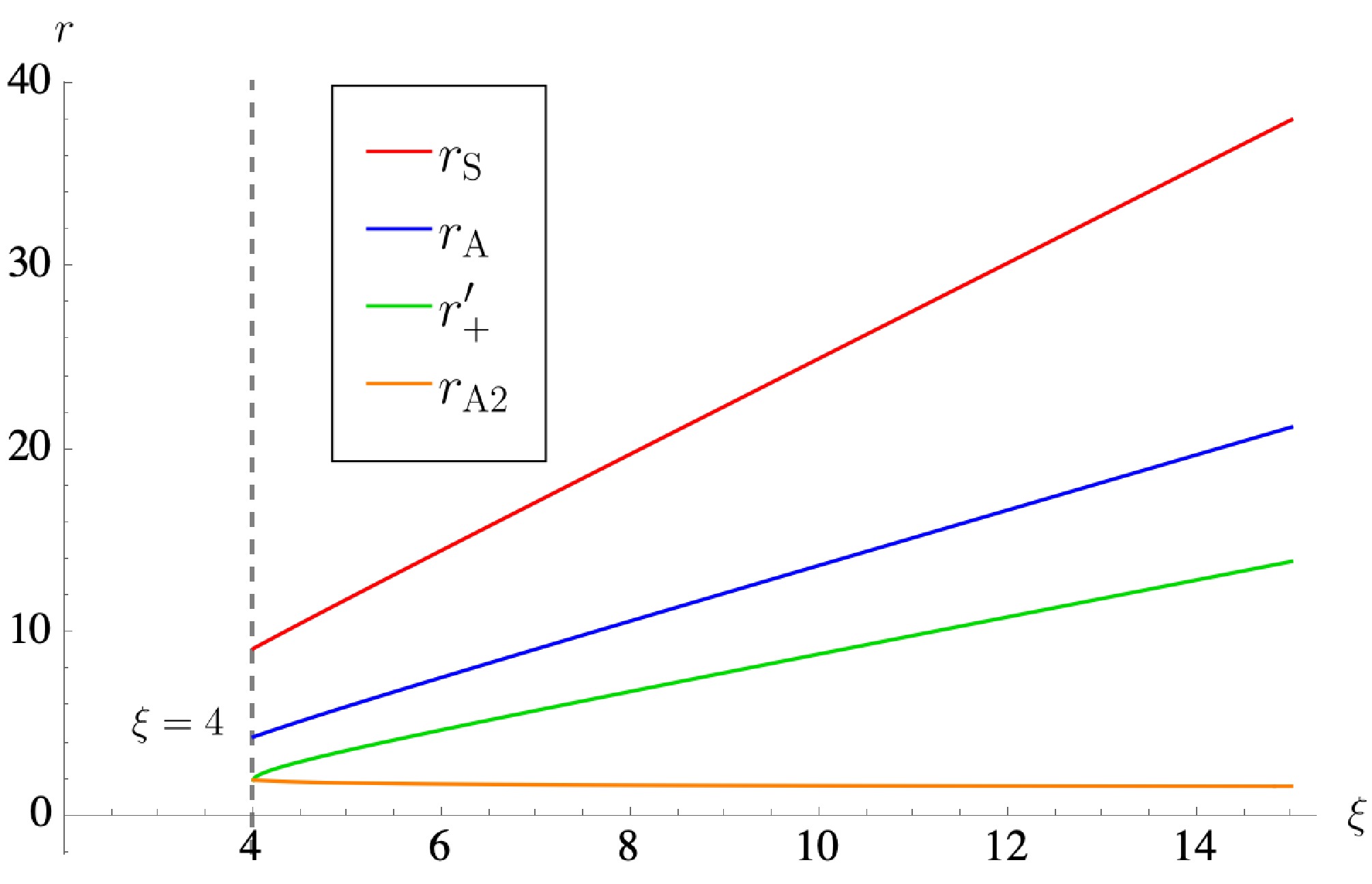

Figure 3.  (color online) Acoustic black hole shadow and associated radii as functions of ξ for fixed $ L=L_0 $. The acoustic shadow radius $ r_\text S $, acoustic sphere radius $ r_\text A $, acoustic horizon $ r_+' $, and second-largest acoustic sphere radius $ r_{\text A2} $ are plotted from the critical value $ \xi=4 $ onward.

Given that the acoustic Hayward black hole is spherically symmetric, once the shadow radius $ r_\text S $ is obtained, the approximate image of the black hole shadow can be constructed. By defining $ r_\text S=\sqrt{\alpha^2+\beta^2} $, the shadows are plotted in the $ (\alpha,\beta) $ plane for different parameter choices, as shown in Fig. 4. In the left panel, with $ L=L_0 $ fixed, we plot the acoustic shadow for different values of the tuning parameter $ \xi=4,5,6,7 $. As ξ increases, the black hole shadow also expands. In the right panel, with $ \xi=5 $ fixed, we plot the acoustic shadow for different values of the Hayward parameter $ L=0,\frac{L_0}{2}, L_0,\sqrt{2}L_0 $. The variation in the acoustic shadow with respect to L is relatively small. To highlight this subtle trend, an inset is included, which reveals a slight decrease in the acoustic shadow as L increases. The variation of the acoustic shadow with respect to ξ follows the same pattern as in the acoustic Schwarzschild and charged black hole cases [29, 30], while its dependence on L is consistent with that observed for the Hayward black hole [57].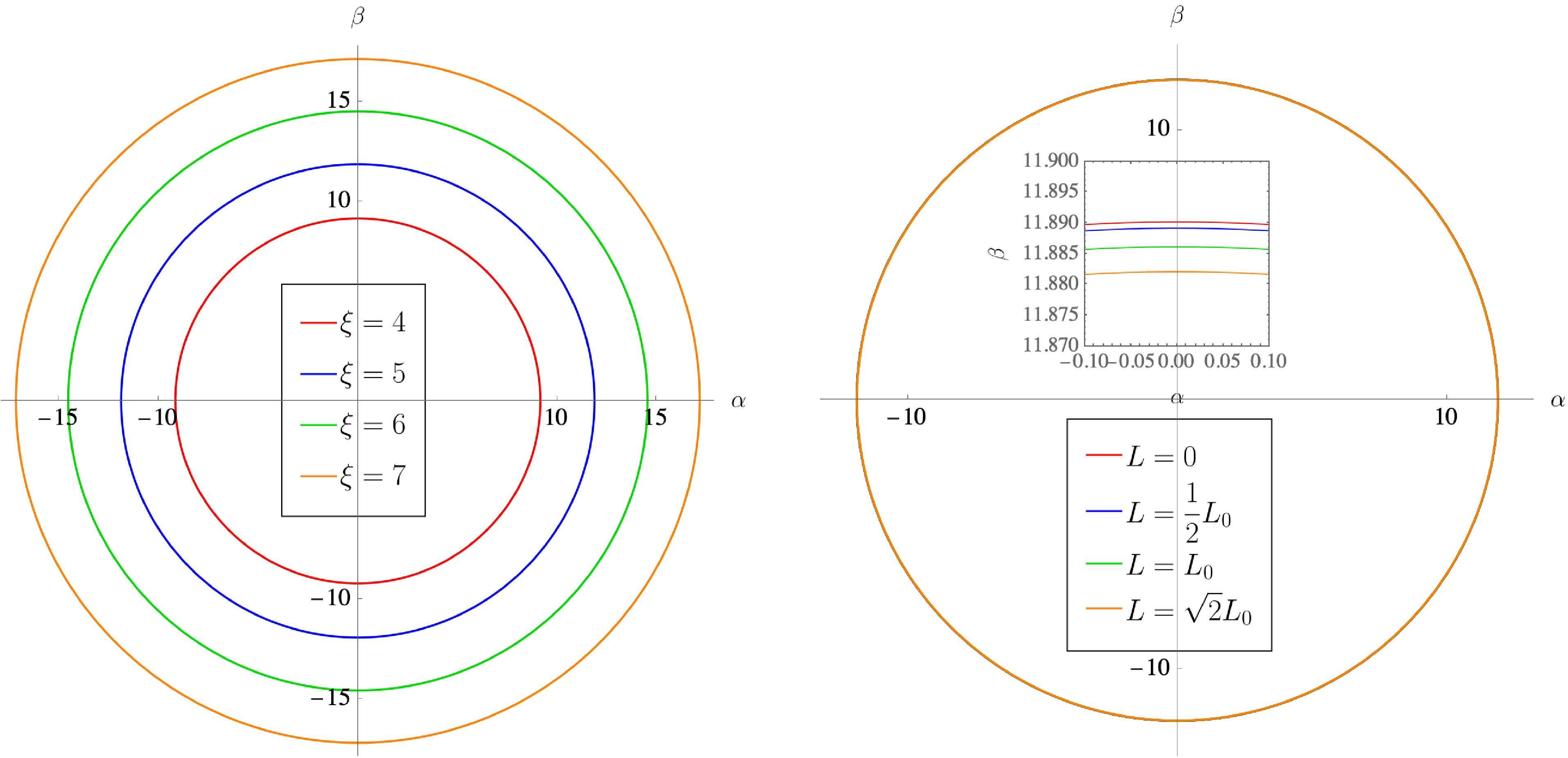

Figure 4.  (color online) Acoustic shadow patterns for different values of ξ and L. Left panel: $ L=L_0 $ is fixed. Right panel: $ \xi =5 $ is fixed, with an inset showing a magnified view of a local region.

Another important property of black holes is their influence on the fields in their vicinity. For instance, black holes can affect the propagation and decay of fields, as manifested in the behavior of QNMs, and can also influence the greybody factor and energy emission rate associated with Hawking radiation. All these phenomena can be studied by solving the equations for test fields near the black hole. Therefore, it is first necessary to derive the covariant field equations in the black hole background. Then, for different physical processes, appropriate boundary conditions are imposed, and the resulting equations are solved accordingly. For acoustic black holes, the fluctuation of the phase $ \theta_1 $ in Eq. (29) is a massless scalar field ψ, i.e., the phonon, satisfying

Using the standard separation of variables, we write

which forms a complete basis. Substituting this ansatz into Eq. (59) and summing over all components yields

where a prime denotes differentiation with respect to r. Introducing the tortoise coordinate defined by $ \mathrm d r_*=\mathcal{F}^{-1} \mathrm d r $, the first two terms combine to give $ \dfrac{ \mathrm d^2\Psi}{ \mathrm d r_*^2} $. The equation then simplifies to

Defining the effective potential as

The covariant equation reduces to a Schrödinger-like equation

The influence of a black hole on a scalar field is largely determined by the form of the effective potential $ V(r) $, shown as a function of r in Fig. 5 and Fig. 6, with the Hayward parameter fixed at $ L=L_0 $ in all cases. In Fig. 5, the angular quantum number is set to $ l=0 $ in the left panel and $ l=1 $ in the right panel, allowing a comparative study of the effective potential $ V(r) $ for different values of the tuning parameter, $ \xi=0,4,5,6 $, where $ \xi=0 $ corresponds to the Hayward black hole. In Fig. 6, the tuning parameter is fixed at $ \xi=5 $ in the left panel and $ \xi=6 $ in the right panel, illustrating the dependence of the effective potential on the angular quantum number l.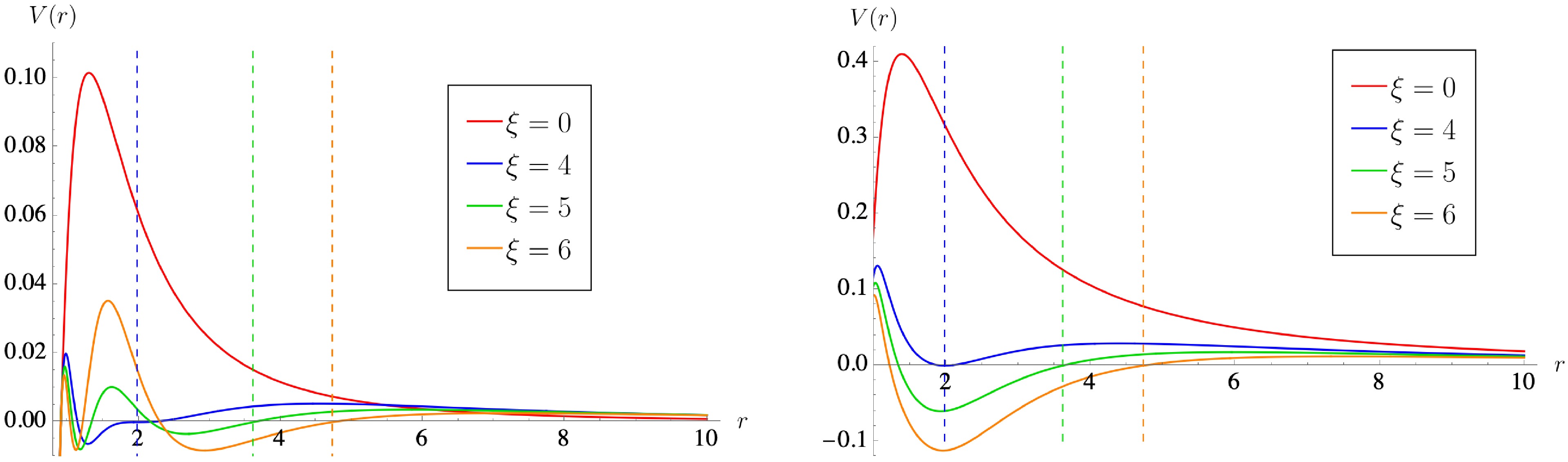

Figure 5.  (color online) The effective potential $ V(r) $ as a function of the radial coordinate r for several values of the tuning parameter ξ, with fixed $ L=L_0 $. Left panel: fixed $ l=0 $. Right panel: fixed $ l=1 $.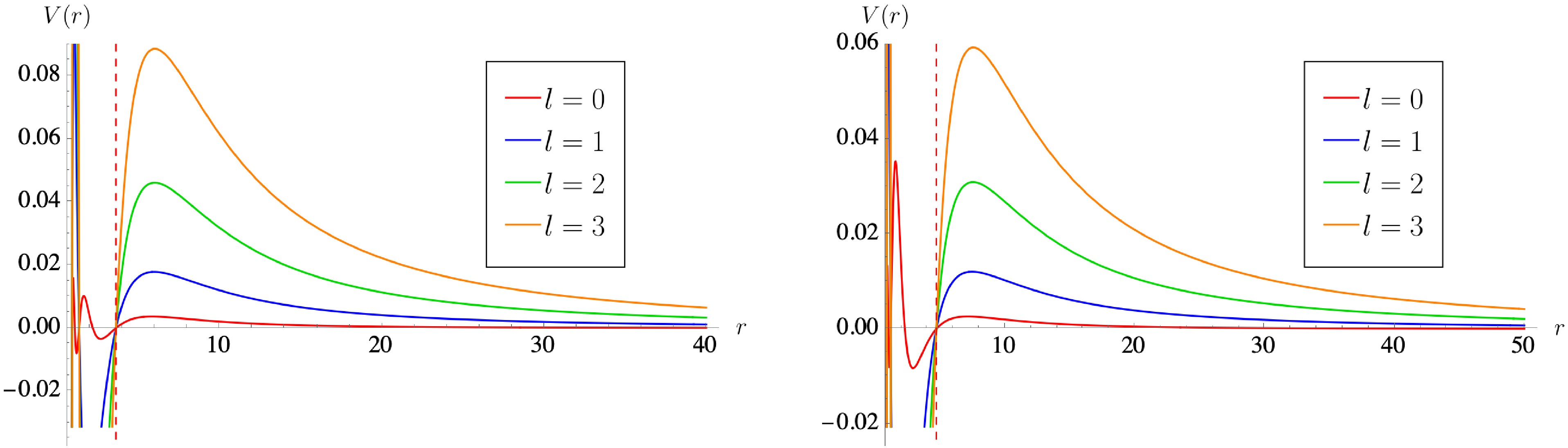

Figure 6.  (color online) The effective potential $ V(r) $ as a function of the radial coordinate r for several values of the angular momentum number l, with $ L=L_0 $ fixed. Left panel: fixed $ \xi=5 $. Right panel: fixed $ \xi=6 $.

In both figures, the effective potential vanishes at the acoustic horizon, marked by the vertical dashed line, exhibits a barrier-like profile outside the horizon, and asymptotically tends to zero at large r. In Fig. 5, as ξ increases, the peak height of the potential barrier decreases. Moreover, the location where the potential vanishes, which corresponds to the acoustic horizon, shifts outward to larger radii, in agreement with the earlier analysis. In Fig. 6, the peak of the effective potential increases with l, while the position at which the potential vanishes remains unchanged, since the radius of the acoustic horizon is independent of the angular quantum number l. The influence of the parameter ξ and the angular quantum number l on the effective potential discussed above will manifest in the subsequent analyses of QNMs and Hawking radiation.

Once the Schrödinger-like equation (64) and the effective potential in Eq. (63) are established, both the QNMs and Hawking radiation can be investigated. We first consider the computation of QNMs. The physical process associated with QNMs can be understood as a "knock" or perturbation outside the black hole, and a QNM, characterized by the complex frequency ω, governs the propagation and decay of this perturbation. In the wave function ψ (59), the temporal dependence takes the form $ e^{-i\omega t}=e^{\text{Im}(\omega)t}e^{-i\text{Re}(\omega)t} $, which implies that:

● The imaginary part, $ \text{Im}(\omega) $, determines the decay (or growth) rate, with $ \text{Im}(\omega)<0 $ corresponding to a decaying mode.

● The real part, $ \text{Re}(\omega) $, gives the oscillation frequency, corresponding to the propagating mode, and is typically taken to be positive, $ \text{Re}(\omega)>0 $.

Accordingly, the appropriate boundary conditions for the wave equation are as follows:

● At the event horizon ($ r_*\rightarrow -\infty $), the waves are purely ingoing, $ \Psi\sim e^{-i\omega r_*} $;

● At spatial infinity ($ r_*\rightarrow +\infty $), the solutions are purely outgoing waves, $ \Psi\sim e^{+i\omega r_*} $.

Due to the complexity of the effective potential (63), we employ the WKB method [58] to compute the QNMs numerically and validate the results using the asymptotic iteration method (AIM) [59, 60]. The WKB method is based on performing a WKB expansion of Ψ near the event horizon and at spatial infinity, i.e., for $ r_*\rightarrow \pm\infty $ [61, 62]. A Taylor expansion of $ Q(r_*)=\omega^2-V(r) $ is carried out around the peak of the effective potential, allowing Ψ to be expressed in terms of parabolic cylinder functions $ D_\nu $, where

where $ Q_0=Q|_{r=r_{0}} $ is the maximum value of $ Q(r_*) $, $ Q_0'=\dfrac{ \mathrm d}{ \mathrm d r_*}Q_0 $, and $ \Lambda_i $ are higher-order correction terms. Explicit expressions for $ \Lambda_2,\Lambda_3 $ can be found in [63], those for $ \Lambda_4-\Lambda_6 $ in [64], and those for $ \Lambda_7-\Lambda_{13} $ in [65]. The integer N is referred to as the WKB order. By analyzing this solution asymptotically and matching it to the WKB expansions, the scattering matrix (S matrix) can be derived [61]. The boundary conditions for QNMs require that $ \Gamma(-\nu) $ in the S matrix be singular. Consequently, ν must be an integer. Eq. (65) therefore gives the WKB formula for ω:

where n is called the overtone number. We use the Mathematica code provided in [58] to compute the QNMs. The results converge well in the sixth-order WKB approximation; nevertheless, we carry out the calculation up to ninth order to improve accuracy.

The results for the tuning parameter $ \xi\leqslant 10 $ are shown in Tabs. 1, 2, and 3, where Tab. 1 corresponds to the mode $ n=0, l=0 $, Tab. 2 to $ n=0, l=1 $, and Tab. 3 to $ n=1, l=1 $. In each table, we present the QNMs computed using the ninth-order WKB method and AIM.

The universal properties of the QNM frequencies are summarized as follows:

● In all modes, the real part satisfies $ \text{Re}(\omega)>0 $, and the imaginary part satisfies $ \text{Im}(\omega)<0 $, indicating that the acoustic Hayward black hole remains stable under perturbations for small ξ, as established earlier. This is consistent with the behavior of the Hayward black hole [47, 66].

● The QNM amplitudes of the acoustic Hayward black hole with $ \xi\geq 4 $ are significantly smaller than those of the Hayward black hole with $ \xi=0 $. This indicates that the QNM signals are weaker in an acoustic black hole than in an astrophysical black hole, which is consistent with previous findings [29, 30].

● As ξ increases, the real part and the magnitude of the imaginary part of the QNMs decrease. This means that both the oscillation frequency and the decay rate decrease, which can be attributed to the suppression of the effective potential and the alteration of the spacetime geometry as ξ increases, as shown in Fig. 5 and Eq. (34). This decrease persists for $ \xi>10 $, as will be shown in Figs. 8 and 7.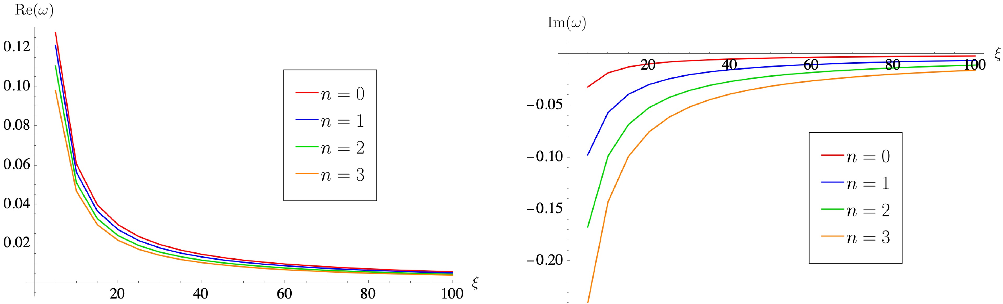

Figure 8.  (color online) QNM frequencies as functions of ξ for different overtone numbers n at fixed $ l=1 $: real parts (left panel) and imaginary parts (right panel).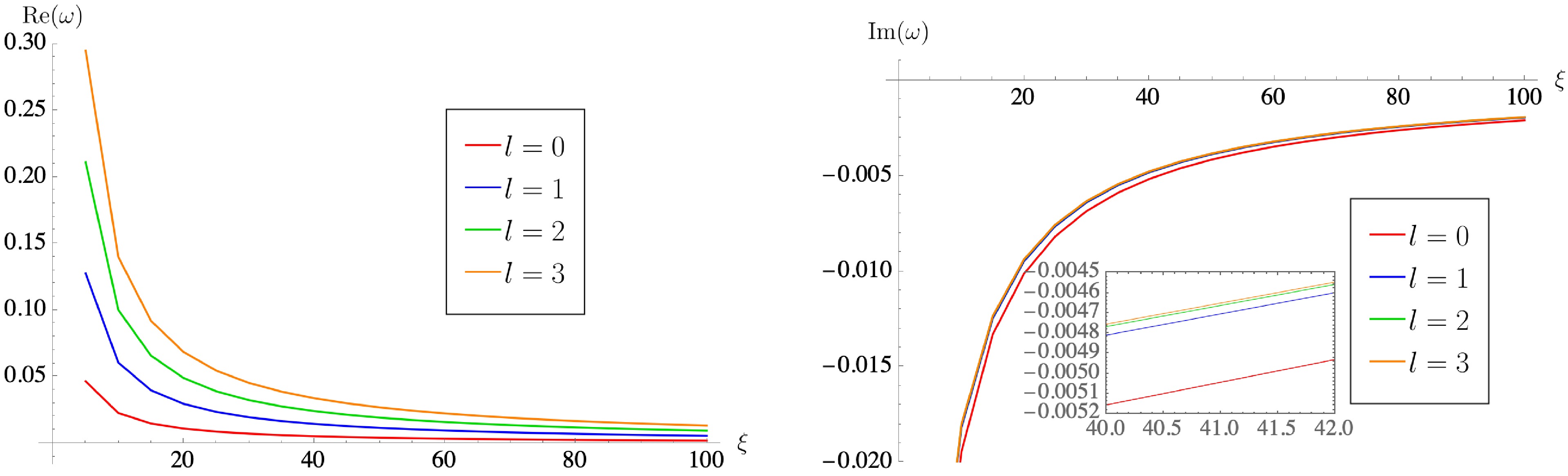

Figure 7.  (color online) QNM frequencies as functions of ξ for different angular numbers l at fixed $ n=0 $: real parts (left panel) and imaginary parts (right panel). A magnified view is shown in the inset of the right panel.

● In each table, the results obtained using the AIM and WKB methods show only minor discrepancies, confirming the accuracy of the WKB calculations.

In addition to presenting the values of the QNMs for $ \xi\geq 10 $, we further investigate their behavior at larger ξ for different overtone numbers n and angular momentum numbers l, as illustrated in Figs. 7 and 8. In Fig. 7, with n fixed at $ 0 $, the dependence of the QNMs on ξ is plotted for $ l=0,1,2,3 $. Conversely, Fig. 8 shows the evolution of the QNMs with ξ for $ n=0,1,2,3 $, while keeping $ l=1 $ fixed. In both figures, the left and right panels display the real and imaginary parts of the QNMs, respectively.

The following conclusions can be drawn from these figures:

● In Figs. 7 and 8, it is evident that, for all combinations of n and l considered, the real part of the QNM frequencies remains positive, while the imaginary part remains negative. This indicates the stability of the acoustic Hayward black hole. Moreover, both the real and imaginary parts tend toward zero as ξ increases, consistent with the preceding discussion.

● In Fig. 7, as the angular momentum number l increases, the real part of the frequency increases, and the magnitude of the imaginary part of the frequency decreases. This trend is attributed to the corresponding reduction in the effective potential for higher l, as shown in Fig. 6.

● In Fig. 8, as the overtone number n increases, the real part $ \text{Re}(\omega) $ decreases, while the magnitude of $ \text{Im}(\omega) $ increases. This indicates a reduction in the oscillation frequency together with an enhanced damping rate, consistent with the behavior of other acoustic black holes [29, 30].

The WKB method can be used not only to numerically calculate the QNM frequencies but also to reveal the geometric correspondence between QNMs and unstable circular null geodesics in the eikonal limit [67]. In the eikonal limit ($ l\gg 1 $), the effective potential in Eq. (63) becomes

According to Eq. (66), the first-order WKB formula is

where $ V_0=V|_{r=r_{0}} $ is the extremum of the effective potential, and $ V_0'=\dfrac{ \mathrm d}{ \mathrm d r_*}V_0 $. Furthermore, $ r_0 $ is actually the radius of the acoustic sphere $ r_\text A $, since it also satisfies the condition (53). In the eikonal limit, the QNM frequency can be written as $ \omega=l\Omega_c-i\left(n+\dfrac{1}{2}\right)|\lambda| $ [67], where the specific meanings of the coefficients will be explained later. Thus, the QNM frequencies can be obtained as

Moreover, from Eqs. (50), (54), and (56), we note that the coefficient of l satisfies

which coincides with the definition of the angular velocity $ \Omega_c $ of the acoustic sphere. Moreover, the coefficient of the term $ -i(n+\dfrac{1}{2}) $ is identified as the Lyapunov exponent λ, which reflects the instability of the acoustic sphere since $ \delta r(t)\sim e^{\lambda t} $ [67, 68]. After simplifying the expression for the Lyapunov exponent, one obtains the relationship between the QNMs and the acoustic sphere (and the acoustic shadow) as

where the expressions for the angular velocity $ \Omega_c $ and the Lyapunov exponent λ are

Note that, in the rotating black hole case, the loss of spherical symmetry leads to a slightly different form of this formula [68, 69]. Based on the analysis of the acoustic sphere and acoustic shadow in Sec. III, we computed the QNM frequencies in the eikonal limit and compared the results with those obtained using the 9th-order WKB approximation. We varied l from 200 to 800 and present the relative errors of the real and imaginary parts obtained by the two methods in Tab. 4. The results confirm that, in the eikonal limit, the relation between the acoustic shadow (and acoustic sphere) and QNMs remains valid for acoustic Hayward black holes. Both the real and imaginary parts of the QNM frequencies obtained in the eikonal limit exhibit only minor deviations from the WKB results, and these errors continue to decrease as l increases, thereby verifying the validity of the correspondence in Eq. (71).

In addition to QNMs, Hawking radiation can also be studied by solving the covariant field equations (64). As with conventional black holes, acoustic black holes emit analogue Hawking radiation and, correspondingly, possess an analogue Hawking temperature [11]. The underlying physical process of Hawking radiation can be understood as a wave originating near the horizon, which is then scattered by the effective potential. Part of the wave is reflected back, while another part tunnels through the potential barrier and reaches spatial infinity. Thus, Hawking radiation can be formulated as a scattering problem with the following boundary conditions:

● Near the event horizon ($ r_*\rightarrow -\infty $), $ \Psi=e^{-i\omega r_*}+R_l(\omega)e^{+i\omega r_*} $.

● At spatial infinity ($ r_*\rightarrow +\infty $), we have $ \Psi=T_l(\omega)e^{-i\omega r_*} $.

Here, $ R_l(\omega) $ and $ T_l(\omega) $ denote the reflection and transmission coefficients, respectively, which depend on both ω and l and satisfy the relation $ |R_l(\omega)|^2+|T_l(\omega)|^2=1 $. The grey-body factor $ \mathcal{A}_l(\omega) $ for analogue Hawking radiation is exactly the transmission coefficient, yielding $ |\mathcal A_l(\omega)|^2=1-|R_l(\omega)|^2=|T_l(\omega)|^2 $. Therefore, the grey-body factors can be obtained by imposing the scattering boundary conditions on the aforementioned S-matrix [61, 63], namely

where the relation between the overtone number n and ω can be obtained from Eq. (66). The grey-body factors can then be computed numerically using the WKB method [58, 70], which modifies the black-body radiation spectrum as $ \dfrac{ \mathrm d E_{gb}}{ \mathrm d t}=|\mathcal A_l|^2\dfrac{ \mathrm d E_{bd}}{ \mathrm d t} $. Accordingly, the energy emission rate for analogue Hawking radiation is given by [7, 71]

where the analogue Hawking temperature is $ T_H=-\dfrac{\mathcal{F}'(r_{+}')}{4\pi} $. Fig. 9 presents the dependence of the analogue Hawking temperature on ξ and L. In the left panel, with L fixed at $ L_0 $, the temperature initially increases with ξ for $ \xi\geq4 $ and then decreases. The initial rise is attributed to changes in the effective potential peak and the energy emission rate, whereas the subsequent decline results from the alteration of the spacetime geometry. In the right panel, with ξ fixed at $ \xi=5 $, the analogue Hawking temperature decreases as L increases over the range $ 0\leqslant L\leqslant \sqrt{2}L_0 $. This reduction similarly arises from the suppression of the energy emission rate, which will be discussed in detail later.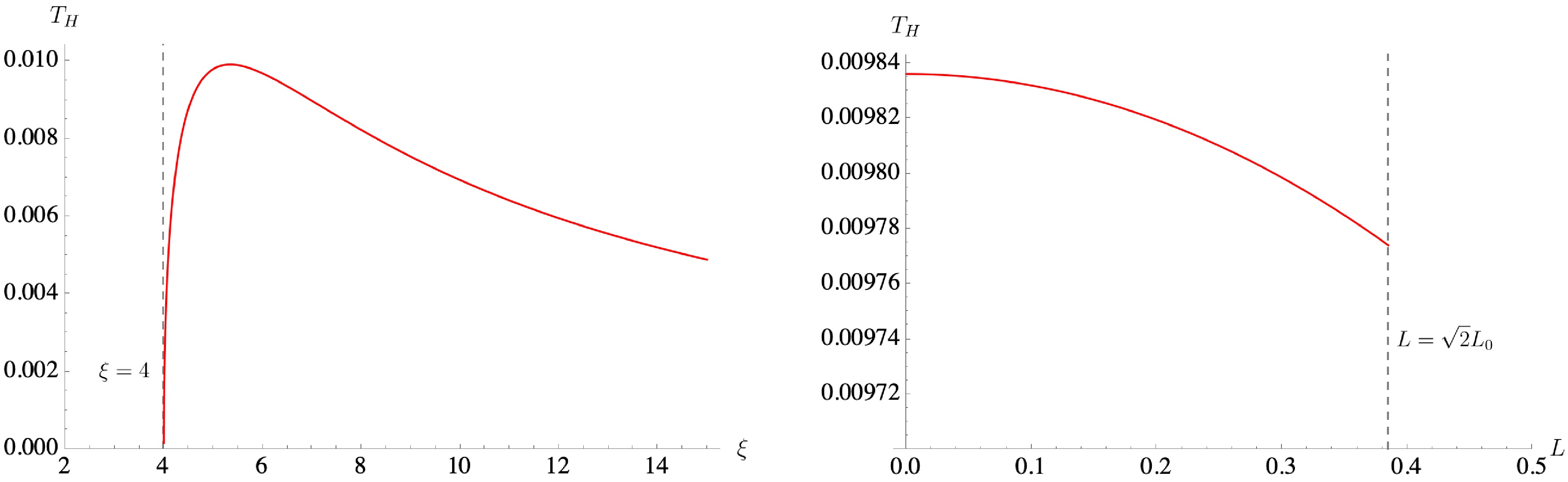

Figure 9.  (color online) Analogue Hawking temperature as a function of ξ for $ \xi \geq 4 $ with $ L = L_0 $ (left panel), and as a function of L for $ 0 \leqslant L \leqslant \sqrt{2}L_0 $ with $ \xi = 5 $ (right panel).

The grey-body factors and energy emission rates for the analogue Hawking radiation of the acoustic Hayward black hole are calculated using the 6th-order WKB approximation, as shown in Figs. 10, 11, and 12. In these figures, the left panels show the grey-body factors, while the right panels display the energy emission rates, both plotted as functions of the frequency ω for different values of the angular momentum number l, the parameter ξ, and the Hayward parameter L. Specifically, Fig. 10 corresponds to fixed parameters $ \xi=5 $ and $ L=L_0 $, with results displayed for different values of $ l=0,1,2,3 $. Fig. 11 shows the behavior for $ L=L_0 $ and $ l=1 $, considering different values of $ \xi=4,5,6,7 $. Meanwhile, Fig. 12 displays the results for fixed $ l=0 $ and $ \xi=5 $, showing the dependence on L with values $ L=0,\dfrac{1}{2}L_0,L_0, $ and $ \sqrt{2}L_0 $.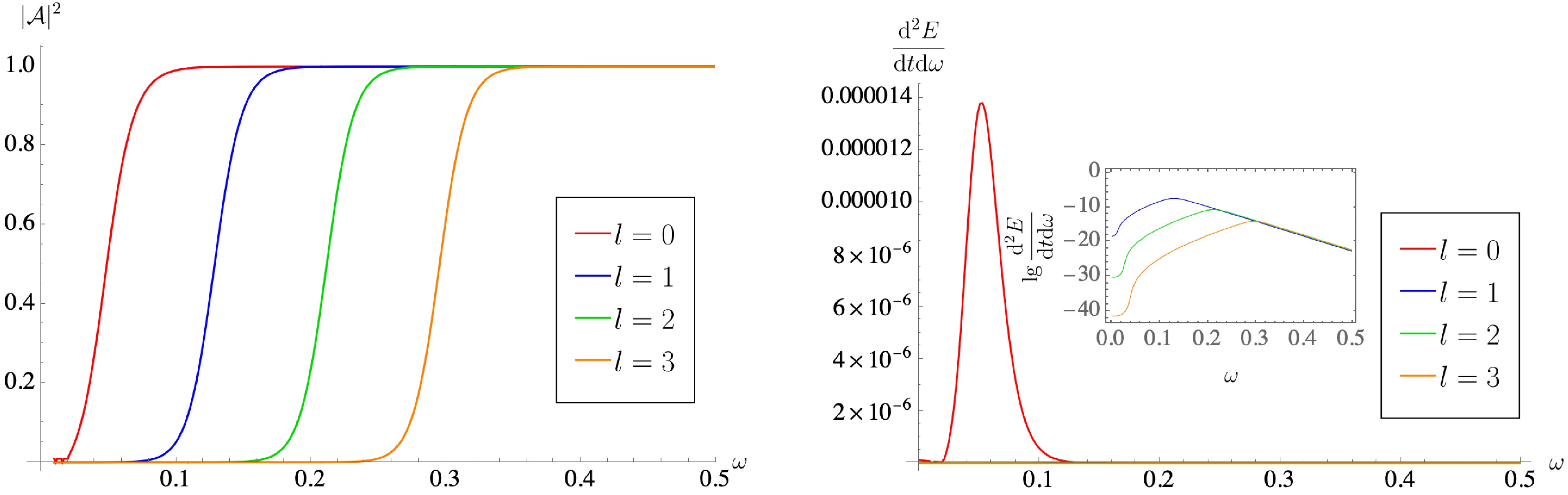

Figure 10.  (color online) Greybody factor (left panel) and energy emission rate (right panel) as functions of ω for different values of l, with $ \xi=5 $ and $ L=L_0 $. The inset in the right panel shows a logarithmic plot of the emission rate, highlighting the detailed features.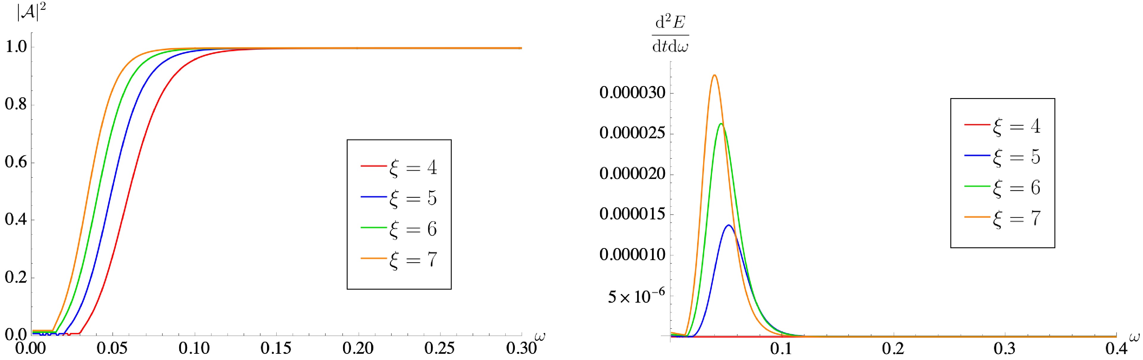

Figure 11.  (color online) Greybody factor (left panel) and energy emission rate (right panel) as functions of ω for different values of ξ, with $ l=0 $ and $ L=L_0 $.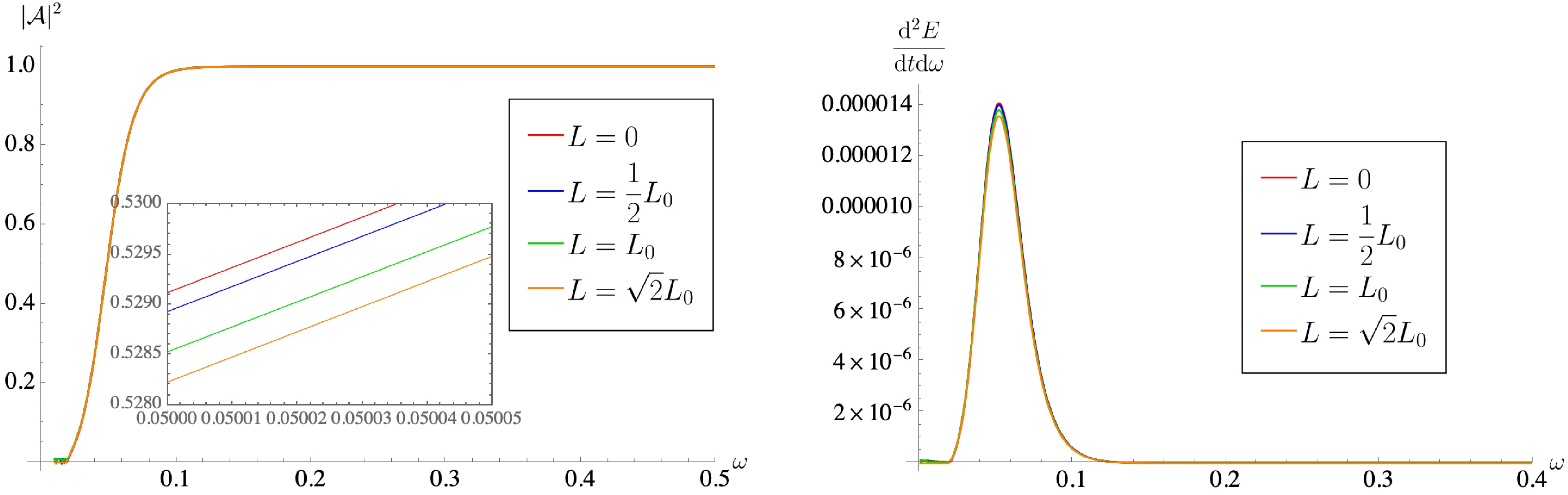

Figure 12.  (color online) Grey-body factor (left panel) and energy emission rate (right panel) as functions of ω for different values of L, with $ l=0 $ and $ \xi=5 $. A magnified view is shown in the inset of the left panel.

Based on the presented results, the following conclusions can be drawn:

● In all cases, the grey-body factors for each mode begin at zero in the low-frequency limit and asymptotically approach unity as the frequency increases. This trend reflects the fact that higher-frequency particles possess greater energy, making them more likely to tunnel through the potential barrier. Similarly, for every mode, the energy emission rate exhibits a distribution analogous to the blackbody radiation spectrum: it vanishes in both the low- and high-frequency limits, with a single peak occurring at intermediate frequencies. This behavior arises because the grey-body factor approaches zero at low frequencies, while the probability of producing high-energy particles becomes extremely small in the high-frequency regime. These findings are consistent with the results obtained for the Hayward black hole [72].

● In Fig. 10, the left panel shows that as the angular momentum number l increases, the grey-body factor saturates more slowly. This behavior can be explained by the increase in the effective potential barrier height with l, as shown in Fig. 6, and indicates that the dominant contribution to the analogue Hawking radiation originates from the zero-angular-momentum modes.

● In Fig. 11, for a fixed angular momentum quantum number l, both the grey-body factor and the energy emission rate increase with ξ. This behavior arises because a larger value of ξ corresponds to a lower effective potential barrier, as shown in Fig. 5.

● In Fig. 12, we examine how the Hayward parameter L influences Hawking radiation. As L increases, both the grey-body factor and the energy emission rate of analogue Hawking radiation decrease slightly, which is consistent with the conclusion drawn from Fig. 9. This modest variation occurs because L is constrained to the narrow range $ 0\leqslant L\leqslant \sqrt{2}L_0 $, which is specific to the Hayward metric.

In this paper, we constructed the acoustic black hole within the Hayward spacetime using the relativistic GP theory, thereby presenting the first extension of acoustic black holes to a regular black hole spacetime. We analyzed the horizon structure of this acoustic Hayward black hole and investigated how the acoustic and Hayward horizons vary with the tuning parameter ξ and the Hayward parameter L. It was shown that the acoustic horizon size increases with ξ but decreases slightly with L. Based on this, we investigated the acoustic shadow of the acoustic Hayward black hole. The formation mechanism of the black hole shadow was explained, and its radius was computed by analyzing the critical null geodesics. Our results provided shadow images for different values of ξ and L, indicating that the shadow size increases with ξ but decreases slightly for larger L.

Moreover, we analyzed the QNMs and analogue Hawking radiation of the acoustic Hayward black hole. By reducing the covariant scalar field equation near the black hole to a Schrödinger-like form, the effective potential was shown to exhibit a potential-barrier-like profile for all parameter values considered, vanishing both at infinity and at the horizon. In addition, the height of the effective potential decreases as ξ increases and rises with the angular momentum number. These features are important for the subsequent calculation of QNMs and analogue Hawking radiation.

Then, by imposing appropriate boundary conditions on the scalar field equation, we computed the QNM frequencies numerically using the WKB method. A WKB expansion of the scalar field yields the scattering matrix, and applying the boundary conditions to the scattering matrix leads to a WKB expression for the QNM frequency ω. Implementing the 9th-order WKB approximation in Mathematica, we obtained the QNMs for different overtone numbers n and angular momentum numbers l. These results were further validated with the AIM. It was shown that the real part of the QNM frequency is positive and the imaginary part is negative for all modes considered, confirming the stability of the acoustic Hayward black hole. As l increases and n decreases, the real part of the QNM frequency grows, while the magnitude of its imaginary part diminishes. This trend demonstrates how the acoustic Hayward black hole affects scalar fields of different modes, consistent with the corresponding variations in the effective potential. Furthermore, we also verified the relationship between the QNM frequencies and the acoustic sphere (and the acoustic shadow) in the eikonal limit. The results indicated that this relationship also holds for the acoustic Hayward black hole.

Finally, by applying scattering boundary conditions to the phonon, we investigated the analogue Hawking radiation of the acoustic Hayward black hole. We examined how the analogue Hawking temperature depends on the parameters ξ and L, and showed that the temperature initially increases and then decreases with increasing ξ, while it exhibits a gradual decline as L increases. Using the 6th-order WKB approximation, we computed the grey-body factors and energy emission rates. It was shown that an increase in the angular momentum number l leads to a suppression of both the grey-body factor and the emission rate, which is explained by the corresponding change in the effective potential. Notably, the dominant contribution to the analogue Hawking radiation comes from the $ l=0 $ mode. As the parameter ξ increases, the grey-body factors and emission rates are enhanced, a trend that follows the rise in temperature and is likewise linked to the evolution of the effective potential. Moreover, as L increases, both the grey-body factor and the energy emission rate of analogue Hawking radiation exhibit a slight decrease.

Our results demonstrated that the acoustic shadow provides a directly observable quantity, offering a potential experimental probe for simulating and detecting acoustic black holes. By analyzing the acoustic shadow, one can effectively uncover the geometric and dynamical properties near the acoustic horizon, thereby deepening the understanding of gravitational effects in the vicinity of black holes. We focused on the influence of the singularity on acoustic black holes. By comparing the results for $ L=0 $ and $ L>0 $, it was shown that the acoustic Schwarzschild black hole exhibits a larger acoustic shadow, a higher analogue Hawking temperature, and stronger analogue Hawking radiation compared to the acoustic Hayward black hole. Although the difference is small, it may be possible to identify the effects of L in future experiments. In addition, it was shown that for both acoustic and standard Hayward black holes, the variation of observables with the parameter L follows a consistent pattern, reflecting the intrinsic nature of Hayward spacetime. Our work constructed an acoustic black hole model in a singularity-free black hole background, which not only expands the study of analogue gravity phenomena but also explores acoustic wave propagation in complex media near regular black holes, thereby providing potential applications for distinguishing regular black holes from black holes with singularities in future astronomical observations via acoustic black hole effects.

Building on the current findings, several promising directions for future research emerge. First, the construction of acoustic black holes can be extended to other types of regular black holes, such as those from loop quantum gravity [73], thus enabling comparisons of the QNMs and acoustic shadows of acoustic black holes in different regular black hole spacetimes. Second, extending the acoustic regular black hole into the holographic framework and studying its connection with real gravity represents a natural and promising direction [74, 75]. Third, since astrophysical black holes are typically rotating, the acoustic black hole framework can be extended to rotating acoustic regular black holes. It would be valuable to investigate acoustic shadows, QNMs, and analogue Hawking radiation in rotating regular black hole cases, with a particular focus on the correspondence between unstable circular null geodesics and QNMs in the eikonal limit. Finally, replacing the fluid near astrophysical black holes with plasma accretion [33] is also a promising direction, which will bring the model closer to real astrophysical black holes and provide useful theoretical support for future related observations.