A novel realization of linear seesaw model in a non-invertible selection rule with the assistance of $\mathbb{Z}_3$ symmetry

The existence of tiny but nonzero active neutrino masses provides a clear hint of physics beyond the Standard Model (BSM), and extensive literature has been devoted to explaining the smallness of neutrino masses. Along these lines, the Linear Seesaw (LSS) [1–3] and the Inverse Seesaw (ISS) [1, 4] are well-known testable scenarios that generate tiny neutrino masses at the TeV scale, predicting tiny Majorana mass matrices for sterile neutral fermions. The smallness of these masses is protected by an approximate lepton-number symmetry, since lepton-number violation induces the tiny active neutrino masses. This type of mechanism for explaining small parameters is referred to as technical naturalness in the 't Hooft sense. The model includes right-handed and left-handed neutral fermions, $ N_R $ and $ N_L $, respectively. After spontaneous electroweak symmetry breaking, one generally writes the following mass terms:

where $ m_{D}\equiv y_d v/\sqrt2 $ and $ m'_D \equiv y'_d v/\sqrt2 $. Here, v is the vacuum expectation value (VEV) of the SM Higgs boson H, denoted by $ \langle H\rangle\equiv [0,v/\sqrt2]^T $. The mass matrix for the neutral fermions in the basis $ [\nu_L^C,N_R, N_L^C]^T $ is given by

If we impose the mass hierarchies as

One finds the following active neutrino mass matrix:

If the first two terms dominate, the model is called the LSS; if the last two terms dominate, the model is called the ISS. Given that the active neutrinos mix with moderately heavy neutral fermions, non-unitarity constraints become relevant. One must take into account several experimental results, such as the effective Weinberg angle, the SM W boson mass, several ratios of Z boson fermionic decays, the invisible decay of the Z boson, electroweak universality, measurements of the quark mixing matrix, and lepton flavor violation (LFV). The constraints are summarized in terms of $ \epsilon\equiv m'^*_D (M^\dagger_N)^{-1} M^{-1}_N m'^T_D+m^*_D (M^*_N)^{-1} (M^T_N)^{-1} m^T_D $ [5]:

where $ |\epsilon| $ denotes the absolute values of the matrix elements. These constraints require the scales of $ m_D $ and $ m'_D $ to be much smaller than that of $ M_N $:

However, from a theoretical perspective, there is no satisfactory explanation as long as one remains within the simplest model.

In this paper, we propose a theoretical explanation for Eq. (7) by introducing a non-invertible symmetry known as the $ {\mathbb{Z}_3} $ Tambara-Yamagami fusion rule ¹, assisted by a discrete Abelian symmetry $ \mathbb{Z}_3 $ and new particles beyond the Standard Model (BSM). In our framework, the mass terms $ m_D $ and $ m'_D $ arise at the one-loop level as leading contributions ², whereas $ M_N $ is allowed at the tree level. This setup leads to rich and verifiable phenomenology, such as LFVs, the anomalous magnetic moments of leptons (lepton $ g-2 $), and a dark matter (DM) candidate. We perform numerical analyses incorporating all relevant phenomenological constraints and present the allowed parameter space of our model for both the normal hierarchy (NH) and inverted hierarchy (IH) of active neutrino masses.

This paper is organized as follows. In Section II, we present our setup and formulate the neutral-fermion mass matrices, discuss LFVs and lepton $ g-2 $, and describe the dark matter candidate and its cross section relevant to the observed relic density. In Section III, we perform a numerical analysis to search for the allowed parameter regions and illustrate the resulting physical trends. Finally, we devote Section IV to the summary and conclusion. We also provide a review of the $ \mathbb{Z}_3 $ TY fusion rule in Appendix A.

Here, we review our model. In addition to the SM fields, we introduce neutral fermions $ N_R $, $ N_L $, $ X_R $, and $ X'_R $, an inert doublet boson $ \eta(\equiv [\eta^+,\eta^0]^T) $, and a singlet inert boson $ S_0 $, with all neutral fermions assumed to have three families for simplicity. Here, $ N_L $ and $ N_R $ are relevant to our linear seesaw model, whereas $ X_R,\ X'_R $, $ \eta,\ S_0 $ play a role in generating the Dirac mass matrices $ m_D $ and $ m'_D $ at the one-loop level after the TY rule is violated. The SM Higgs is denoted by $ H\equiv[w^+,(v+h+i z)/\sqrt2]^T $, where $ w^+ $ and z are absorbed by the SM gauge bosons $ W^+ $ and $ Z_0 $, respectively. We assign TY and $ \mathbb{Z}_3 $ charges to these fields in order to realize the desired model structure. Their field contents and charge assignments are summarized in Table 1. Since H is assigned to $ 1$ under TY and the other bosons, η and $ S_0 $, have vanishing VEVs, TY is not broken spontaneously. However, the TY rule is not a protected symmetry and is broken explicitly at the loop level. Under these symmetries, the Lagrangian in the lepton sector has the following renormalizable terms:

where $ \tilde\eta\equiv i\sigma_2\eta^* $, with $ \sigma_2 $ denoting the second Pauli matrix. Here, we take $ y^\ell,\ M_N,\ M_X $ to be diagonal matrices without loss of generality ³ The scalar potential contains an important term that induces small Dirac mass matrices:

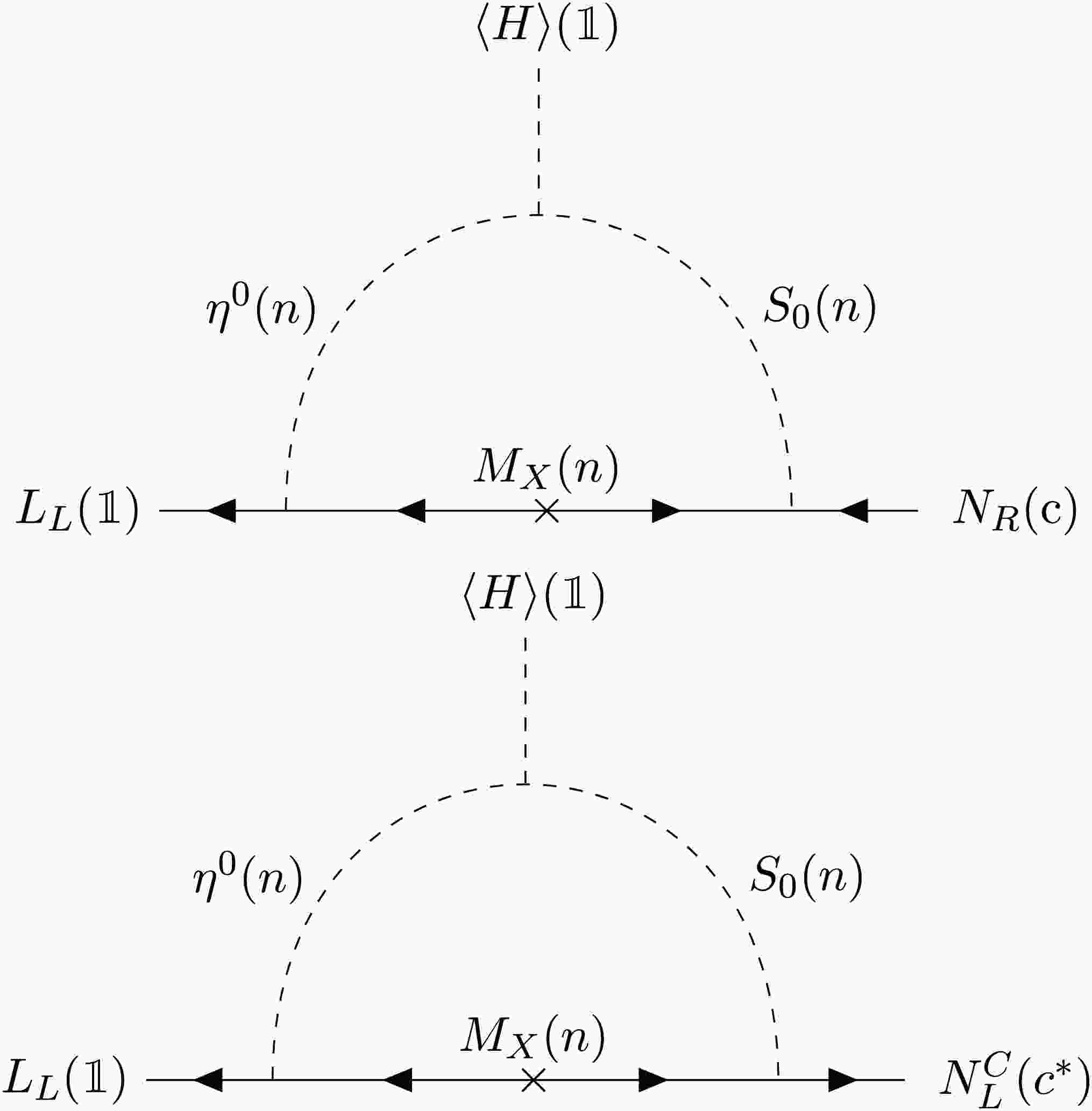
This term, together with $ y^\eta_{i\alpha} $, $ M_{X_{\alpha}} $, and $ y^R_{a\alpha}\ (y^L_{a\alpha}) $, generates the Dirac mass terms $ m_D\ (m'_D) $ at the one-loop level, as shown in Fig. 1. Note that each tree-level interaction is invariant under the TY rule. However, the TY rule is not protected at the loop level and is explicitly broken by these one-loop diagrams; ${ 1}\otimes 1 \otimes c^{(*)}\neq 1 $.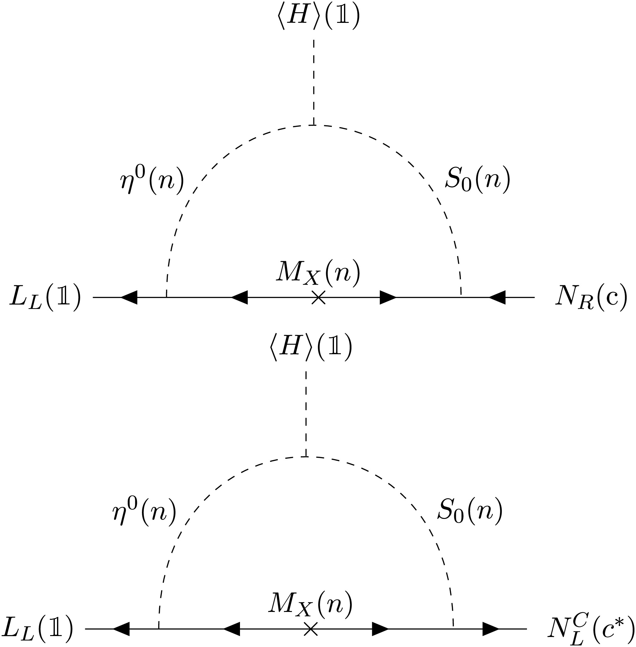

Figure 1.  One-loop diagrams for the Dirac mass matrices, $ m_D $ (up) and $ m'_D $ (bottom). Although the tree-level interactions are invariant under the TY rule, these diagrams are not invariant, since $1\otimes1\otimes{c(c^*)}\neq 1$.

It is worth noting that, at the two-loop level, we obtain a correction to the charged-lepton Yukawa coupling arising from the three terms $ y^\ell,\ y^\eta,\ \mu $. This correction is finite and can therefore be safely neglected.

The TY fusion rule plays an essential role in structuring our linear seesaw model. Below, we list the terms forbidden by the TY rule that would spoil our mass generation mechanism:

However, the TY fusion rules still allow the following terms:

Why is $ Z_3 $ needed? $ Z_3 $ symmetry plays a role in forbidding all the terms in Eq. (14). This is important because these terms generate larger neutrino masses through conventional radiative seesaw mechanisms, thereby spoiling our model. For example, $ (\eta^\dagger H)^2 $ and $ \overline{X^C_{R}} X_{R} $, together with $ y^\eta_{i\alpha} \overline{L_{L_i}} \tilde \eta X_{R_\alpha} $, generate neutrino masses at the one-loop level. Another example ⁴ is $ \overline{L_L} \tilde \eta X'_{R} $ and $ S_0^2 $ with $ M_{X_{\alpha}} \overline{X^C_{R_\alpha}} X'_{R_\alpha} $, $ (\eta^\dagger H)S_0 $, and $ y^\eta_{i\alpha} \overline{L_{L_i}} \tilde \eta X_{R_\alpha} $, which also gives a one-loop contribution. Note here that this $ \mathbb{Z}_3 $ remains unbroken, unlike the symmetry associated with the TY rule.

In addition, we set $ y'^{L,R}=0 $ in the following analysis. Phenomenologically, these terms are harmless since they only generate $ \mu_{L,R} $ in Eq. (2) at the one-loop level, giving higher-order corrections to the active neutrino mass matrix, as we will explain below. Theoretically, however, these one-loop diagrams are divergent and require counterterms. Since such counterterms are forbidden by the TY rule, our model would be spoiled. This problem is resolved by the following argument. If $ y'^{L,R}=0 $ and $ M_X=0 $, $ X'_L $ and $ X'_R $ decouple from the theory, and an additional symmetry is restored. Since $ M_X $ is a dimensionful parameter, it can be generated by a soft breaking of the symmetry in an extended model while maintaining $ y'^{L,R}=0 $ ⁵. This structure also guarantees that, once we set $ y'^{L,R}=0 $ in our model, they are not generated by quantum corrections.

Setting aside the theoretical discussion above for the moment, let us consider the case in which small $ y'^{L,R} $ are generated at a cutoff scale Λ due to some uncontrollable effects, such as gravitational effects. Since these Yukawa couplings are technically natural, they remain small at a low energy scale μ, where we renormalize the theory. These Yukawa couplings generate the mass terms $ \delta \mu_{R_{ab}} \overline{N_{R_a}^C} N_{R_b} $ and $ \delta \mu_{L_{ab}} \overline{N_{L_a}} N^C_{L_b} $ at the one-loop level, which are given by

where $ r_S\equiv m_S^2/\mu^2 $, $ r_{X_\alpha} \equiv M_{X_\alpha}^2/\mu^2 $. These mass terms then generate neutrino masses suppressed by $ 1/(16\pi^2)^3 $ via the inverse seesaw mechanism. Therefore, they are negligible compared with the linear seesaw contributions, which are suppressed by $ 1/(16\pi^2)^2 $.

Here, we discuss the Dirac mass matrices $ m_D $ and $ m'_D $, which are generated at the one-loop level by the diagrams in Fig 1. The resulting contributions are given by

The active neutrino mass matrix is then generated at the two-loop level through the linear seesaw terms in Eq. (4):

which is diagonalized by a unitary matrix $ U_\nu $ as $ (D_1, D_2, D_3)=U^\dagger_\nu m_\nu U^*_\nu $.

Let us impose the following condition for simplicity:

which leads to $ m_D=m'_D $. This can be realized by imposing a reflection symmetry, $ N^C_R\leftrightarrow N_L $. We can then apply the Casas-Ibarra parametrization [37] and use the following expression:

where $ {\cal O} $ is a three-by-three orthogonal mixing matrix with complex entries; $ {\cal O}^T{\cal O}={\cal O}{\cal O}^T=1 $. Since we work in the diagonal basis for the charged-lepton mass matrix, we have $ U\equiv U_{{\rm{PMNS}}}= U_\nu $, where $ U_{{\rm{PMNS}}} $ is the Pontecorvo–Maki–Nakagawa–Sakata (PMNS) matrix [38] with the standard parametrization.

This enables us to solve for $ y^\eta $ as

where it is required to satisfy the perturbative limit $ |y^\eta|\lesssim \sqrt{4\pi} $.

The sum of the neutrino masses $ \sum_i D_i $ has an upper bound of 120 meV [39, 40], assuming the minimal cosmological model. Meanwhile, the recent constraint within ΛCDM is $ \sum D_{i}\le $ 72 meV [41], obtained by combining DESI and CMB data.

The effective neutrino mass for neutrinoless double beta decay, denoted by $ m_{ee} $, is given by

Current KamLAND-Zen data place upper bounds of $ (28-122) $ meV on it at the 90% confidence level [42]. On the other hand, the effective electron antineutrino mass is defined by

It is bounded by a global analysis of oscillation data, in combination with the KATRIN experiment, at 95% CL [43]:

The coupling $ y^\eta $ between the charged leptons and the new particles induces contributions to lepton flavor-violating (LFV) processes and lepton $ g-2 $. The branching ratios for $ \ell_i \to \ell_j \gamma $ are calculated as

where $ \alpha_{{\rm{em}}}\approx1/137 $ is the fine-structure constant, $ {{\rm{BR}}}(\ell_i \to \nu_i \bar\nu_j \ell_j) \approx(1,0.1784, 0.1736) $ gives the branching ratios for $ (i,j)=(\mu,e),(\tau,e),(\tau,\mu) $, respectively, and $ {{\rm{G_F}}}\approx1.17\times 10^{-5} $ GeV$ ^{-2} $ is the Fermi constant.

The contributions to the electron and muon $ g-2 $ are given by

Dark matter candidates in our model are $ X_R $, $ X'_R $, $ \eta^0 $, and $ S_0 $, whose stability is guaranteed by the $ \mathbb{Z}_3 $ symmetry. Here, we regard the lightest $ X_R $ state as the DM candidate, denoted by $ \chi_R $, with mass $ m_\chi $. This case is of particular interest since it interacts only via $ y^\eta $, and thus the dark matter relic abundance is related to the neutrino mass generation mechanism. The cross section for the relic density in the thermal freeze-out scenario is given by

where we expand the cross section in terms of the relative velocity, $ v_{{\rm{rel}}}^2\approx0.2 $ [48], and have used the following relation: $ \sum_{ij}|(U^\dagger y^\eta)_{i1}(U^\dagger y^\eta)_{j1}|=\sum_{ij}\left|y^\eta_{i1}(y^\eta)^\dagger_{1j}\right|^2\equiv |y^{\eta\dagger}y^\eta|_{11}^2 $. To satisfy the observed relic density at $ 2\sigma $ [40], $ 0.118\lesssim\Omega h^2\lesssim 0.122 $, the cross section must lie within the range of

In this section, we perform numerical analyses considering all the constraints discussed above and show the allowed region. Specifically, we consider neutrino oscillation data, non-unitarity bounds, the sum of the neutrino masses, lepton flavor violation constraints, anomalous magnetic dipole moments of leptons, and dark matter with the correct relic density, assuming that one of the $ X_R $ fields has the lightest mass among the DM candidates.

For the analysis, we randomly scan our input parameters within the following ranges:

where we take $ m_{\eta}\equiv m_{\eta^+}=m_{\eta_0} $ to conservatively evade the constraints from the oblique parameters, and $ \alpha,\beta $ are the Majorana phases defined by diag$ [1,e^{i\alpha/2},e^{i\beta/2}] $. Here, $ \tilde\theta_{12,13,23} $ are the complex mixing angles of the orthogonal matrix $ {\cal O} $ in Eq.(23), using the same parametrization as that for $ U_{{\rm{PMNS}}} $. Note that once the lightest neutrino mass is chosen, all neutrino mass eigenvalues are fixed by the experimental values of the neutrino mass-squared differences. We use the best-fit values of the neutrino oscillation data from NuFIT 6.0 [43] for NH and IH.

In Fig. 2, we show the allowed region in the $ m_\eta $–$ m_{S_0} $ plane. Red points indicate parameter sets satisfying 120 meV$ <\sum_i D_i\leq200 $ meV. Blue points represent parameter sets satisfying the stronger condition $ \sum_i D_i\le120 $ meV. We see that $ m_{S_0} $ is scattered over the entire region, whereas $ m_\eta $ appears to have an upper bound of approximately $ 10^4 $ GeV.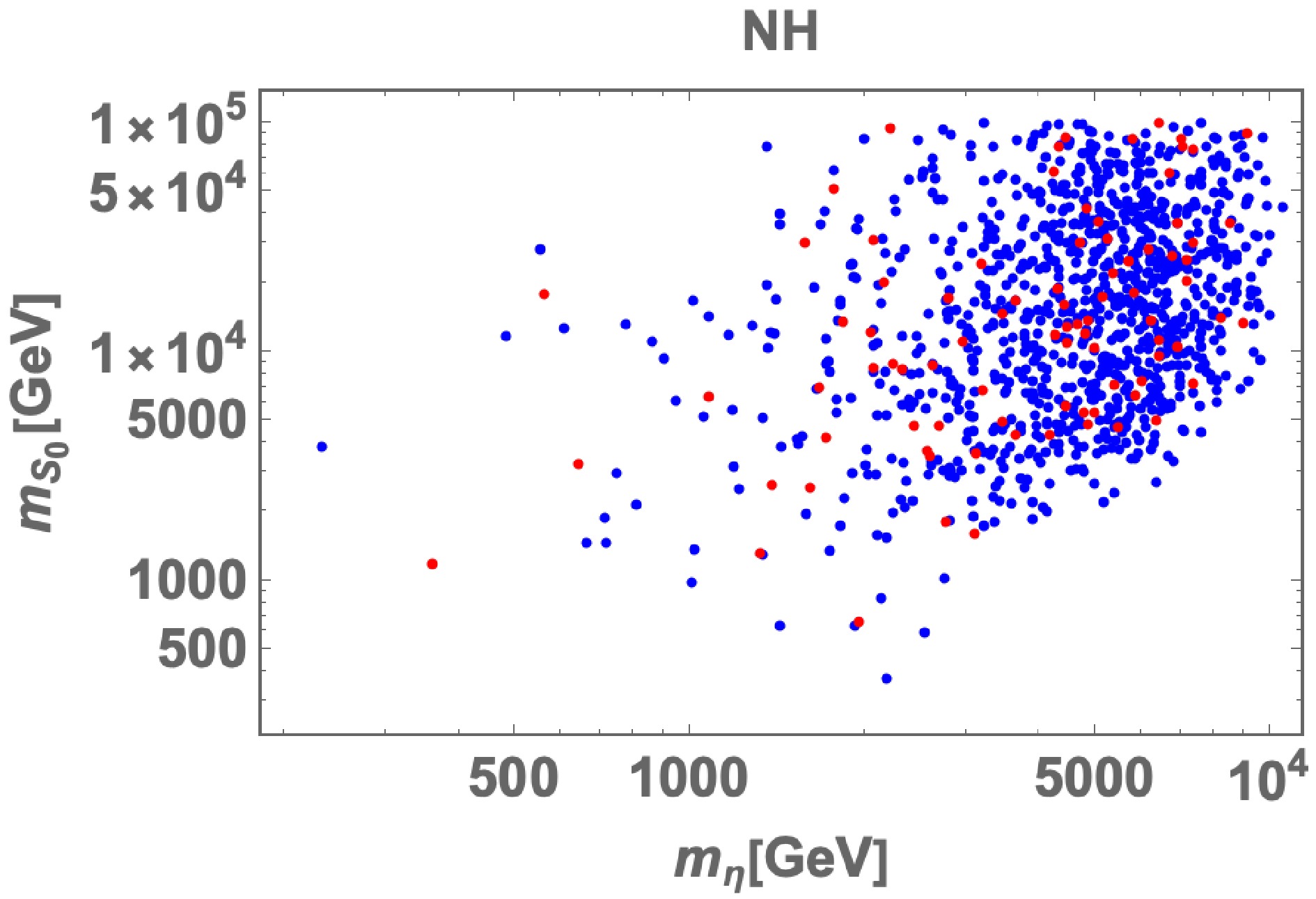

Figure 2.  (color online) Allowed regions of $ m_\eta $ and $ m_{S_0} $ satisfying all the conditions discussed above. Red points indicate parameter sets satisfying 120 meV$ <\sum_i D_i\leq200 $ meV. Blue points represent the subset satisfying the stronger condition $ \sum_i D_i\le120 $ meV.

In Fig. 3, we show the LFV branching ratios for a given DM mass. The figure suggests that many allowed points lie close to the experimental upper limit for $ {{\rm{BR}}}(\mu\to e\gamma) $. The horizontal dotted line represents the future sensitivity of $ {{\rm{BR}}}(\mu\to e\gamma)\le 6\times10^{-14} $ [49], indicating that a significant portion of the parameter space in our model could be ruled out. On the other hand, $ {{\rm{BR}}}(\tau\to \mu\gamma)\simeq10^{-14} $ is favored due to its stronger correlation with $ {{\rm{BR}}}(\mu\to e\gamma) $. Lower values of the DM mass are disfavored by LFV constraints, in particular from $ \mu\to e\gamma $, excluding a large number of model points for $ m_\chi\lesssim500 $ GeV.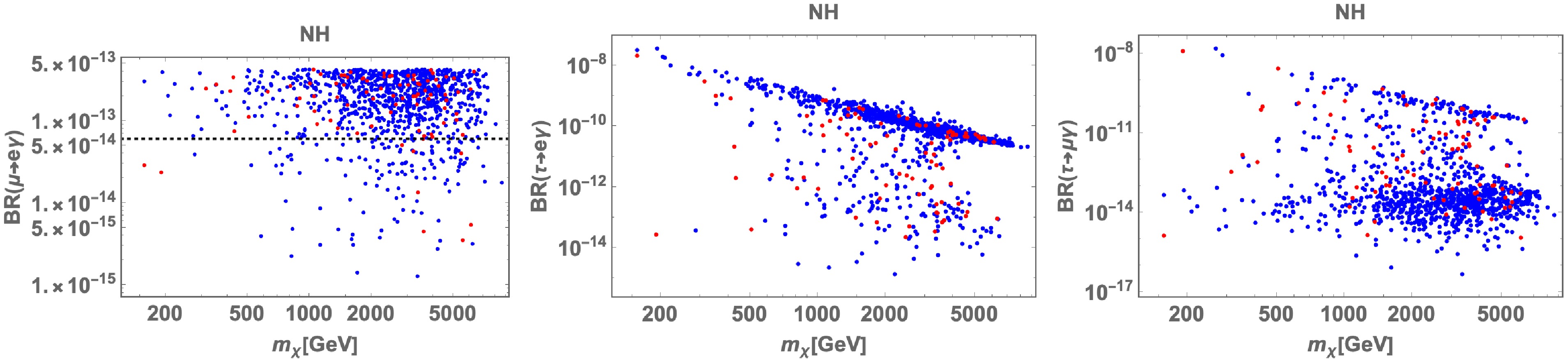

Figure 3.  (color online) Values of LFV observables for a given DM mass. The color legend is the same as that in Fig. 2. The horizontal dotted line represents the projected future sensitivity, BR($ \mu\to e\gamma)\le 6\times10^{-14} $ [49].

In Fig. 4, we show the lepton $ g-2 $ results for a given DM mass. The contributions to both the electron and muon $ g-2 $ are well within the current experimental bounds.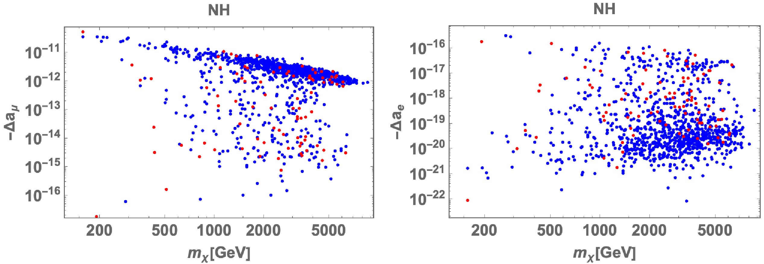

Figure 4.  (color online) Plots of the lepton $ g-2 $ for a fixed DM mass. The color legend is the same as that in Fig. 2.

In Fig. 5, we show the plots related to active neutrino masses. The left panel shows the scatter plot in the $ m_{\nu e} $ and $ \sum_i D_i $ plane. The vertical magenta dashed line represents the upper bound from the combination of DESI and CMB, $ \sum_i D_i\le72 $ meV, while the vertical black line shows $ \sum_i D_i\le120 $ meV. The horizontal black dashed line indicates the lower bound on $ m_{\nu e} $ (0.85 meV). Since $ m_{\nu e} $ does not depend on phases, the scatter points are distributed along a narrow line. The middle panel shows the scatter plot in the $ m_{ee} $ and lightest active neutrino mass $ D_1 $ plane. The horizontal black dashed line indicates the most stringent upper bound on $ m_{ee} $ (28 meV). The yellow region represents the parameter space consistent with the NuFIT 6.0 global fit, excluding other constraints. This figure suggests that almost all the blue points satisfying $ \sum_i D_i\le120 $ meV lie below $ m_{ee}=28 $ meV. The right panel shows the scatter plot in the $ m_{ee} $ and $ \sum_i D_i $ plane. All lines and yellow regions are the same as in the middle panel. This figure implies that many points satisfy $ \sum_i D_i\le72 $ meV.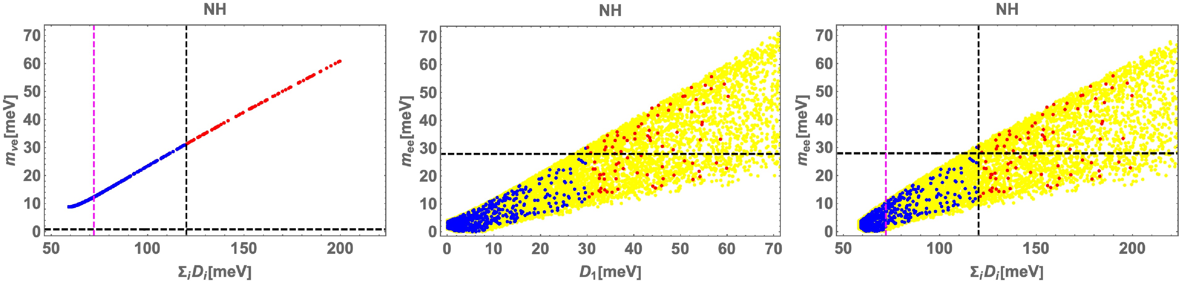

Figure 5.  (color online) Plots of active neutrino masses, with the same color legend as in Fig. 2. The yellow region represents the parameter space consistent with the NuFIT 6.0 global fit.

Figs. 6, 7, 8, and 9 show the corresponding results for the IH case, as in Figs. 2, 3, 4, and 5, respectively. The trends observed in LFV and lepton $ g-2 $ discussed above also appear in the IH case. However, we observe a slight shift in the preferred region in the neutrino sector: the lightest neutrino mass shifts to smaller values, $ D_3\lesssim16 (54) $ meV for $ \sum_i D_i\lesssim 120(200) $ meV; the lower bound on the sum of the neutrino masses becomes stronger, $ 100\ {{\rm{meV}}}\lesssim \sum_i D_i $; and $ m_{ee} $ develops a lower bound, $ 18\ {{\rm{meV}}}\lesssim m_{ee} $, with a weaker dependence on $ D_3 $ and $ \sum_iD_i $.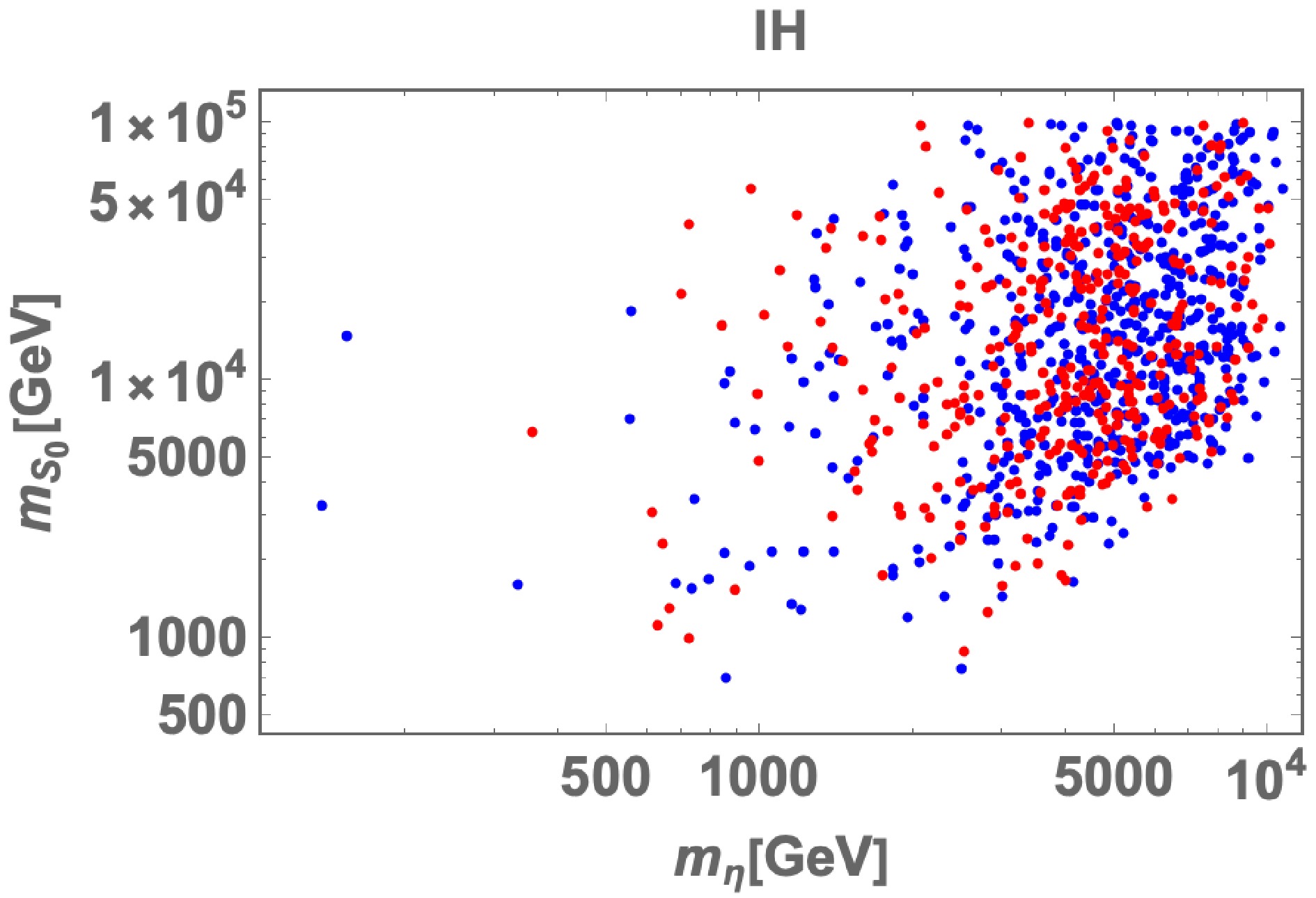

Figure 6.  Same as Fig. 2, but for the inverted hierarchy.

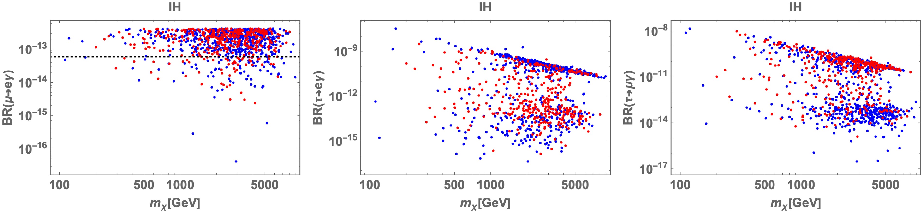
Figure 7.  (color online) The same as Fig. 3, but for the inverted hierarchy.

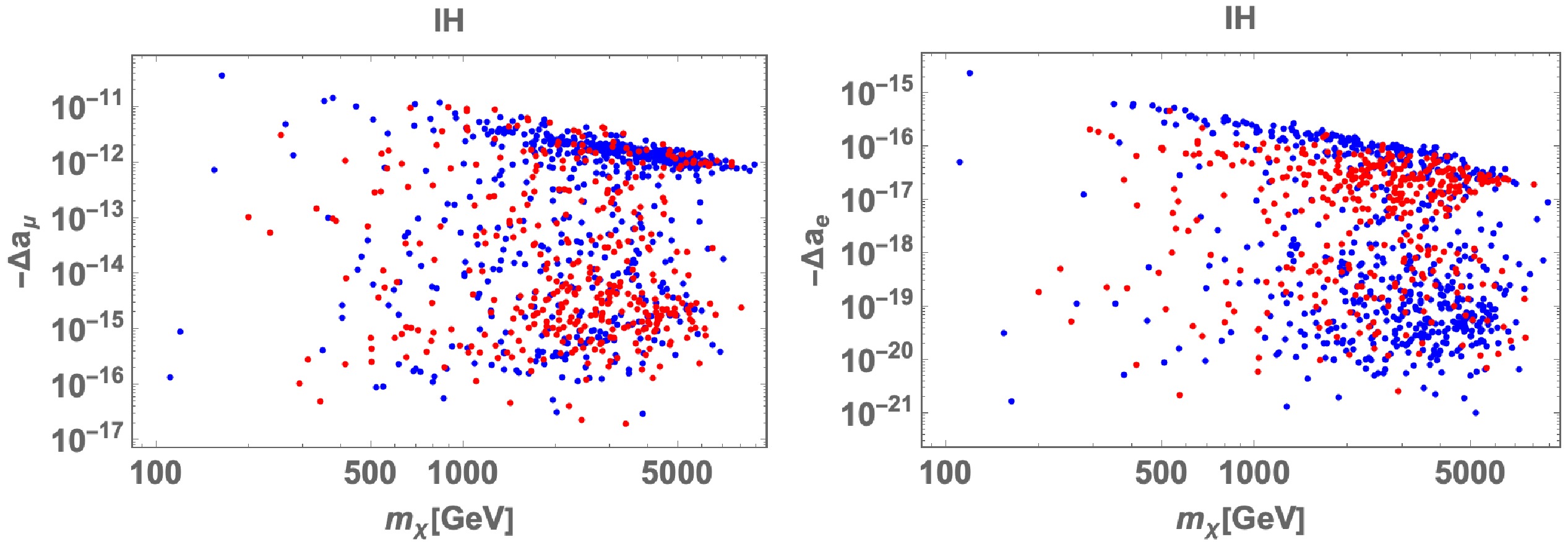
Figure 8.  (color online) Same as Fig. 4, but for the inverted hierarchy.

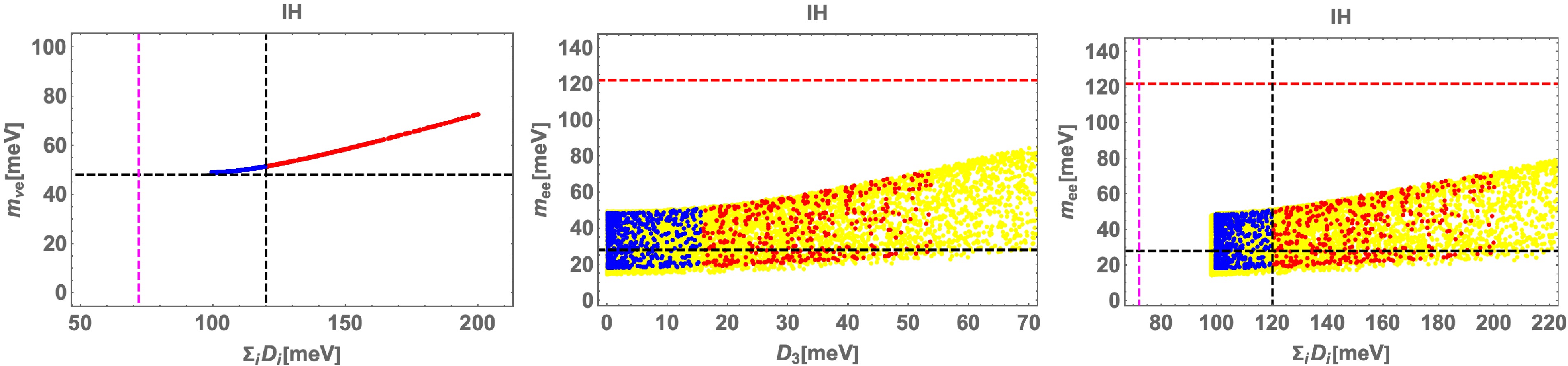
Figure 9.  (color online) Same as Fig. 5, but for the inverted hierarchy.

We have proposed a novel realization of the linear seesaw mechanism based on a $ \mathbb{Z}_3 $ Tambara-Yamagami fusion rule (TY) with the assistance of a $ \mathbb{Z}_3 $ symmetry. In this framework, the mass hierarchies of Eq. (7) are theoretically explained via loop suppression. It is noteworthy that the TY symmetry is broken to generate the hierarchical structure, while it controls the interaction terms needed to realize the structure of the linear seesaw. Owing to this structure, the active neutrino masses are generated at the two-loop level, which naturally predicts new particles around the TeV scale. In addition to the masses and mixings of the active neutrinos, we have also considered lepton flavor violation, lepton $ g-2 $, and dark matter. In particular, we focus on the case in which the lightest Majorana fermion explains the dark matter relic abundance. In our numerical analysis, we have searched for allowed regions satisfying all the constraints: neutrino oscillation data, non-unitarity bounds, three lepton flavor-violating processes, muon/electron $ g-2 $, and the observed relic density of dark matter. We have demonstrated that the model has a large parameter space and identified some tendencies of the observables for NH and IH.

Here, we present the multiplication rules for the Tambara-Yamagami fusion rule associated with $ {\mathbb{Z}_3} $ (TY), where TY consists of four commuting generators, $ \{{ \mathbb{1},c,c^*,n}\} $ $\left[\begin{array}{lll} n \otimes n ={1\oplus c \oplus c^*} \,, ~~~~~ & c \otimes c^* = 1\,, ~~~~~ & c \otimes c =c^* \,, \\[0.3ex] c^* \otimes c^* = c \,, ~~~~~ & c^* \otimes n = c^* \,, ~~~~~ & c \otimes n = c \,.\end{array}\right]$ Note that n is a self-conjugate generator and has no inverse generator.