


 Abstract
 HTML
HTML Reference
 Related
 PDF
PDF


-
Quantum chromodynamics (QCD) is the fundamental theory of the strong interaction. While conventional hadrons are well described as quark-antiquark mesons and three-quark baryons in the quark model [1, 2], QCD also permits the existence of exotic hadron states, such as multiquark states, hybrid mesons, and glueballs. Detailed discussions can be found in recent comprehensive reviews [3−17].
In 2018, the Belle Collaboration first observed a narrow structure, denoted
$ \Omega(2012) $ , in the$ \Xi^{0}K^{-} $ and$ \Xi^{-}K^{0}_{S} $ invariant mass spectra, providing the first experimental evidence for this excited Ω baryon [18]. Prior to this discovery, the mass spectrum of the Ω family had been extensively studied using various theoretical approaches [19−37], many of which predicted a pair of negative-parity excited$ \Omega^- $ states with$ J^P = \dfrac{1}{2}^- $ and$ J^P = \dfrac{3}{2}^- $ in the mass region near 2 GeV. The existence of the$ \Omega(2012) $ was subsequently reinforced by Belle through its observation in weak decays of the$ \Omega_c $ baryon, providing an independent production channel and further consolidating its resonance nature [38]. More recently, the ALICE Collaboration reported the observation of$ \Omega(2012) $ with a significance of$ 15\sigma $ in$ pp $ collisions at the LHC [39], while the BESIII Collaboration presented evidence for a new production mechanism of this state via the process$ e^+e^-\rightarrow \Omega(2012)\bar\Omega^++c.c. $ with a significance of$ 3.5\sigma $ [40, 41]. In the PDG [42], the mass and total decay width of$ \Omega(2012) $ are listed as$ m=2012.4\pm 0.9 $ MeV and$ \Gamma=6.4^{+3.0}_{-2.6} $ MeV, respectively, and the branching fraction ratio is given as$ {\cal{R}}^{\Xi^- \bar{K}^0}_{\Xi^0 K^-} = 0.83\pm 0.21 $ .The discovery of this multistrange resonance has stimulated considerable theoretical interest, focusing on two broad interpretive frameworks. One framework regards
$ \Omega(2012) $ as a conventional excited baryon. In particular, based on its relatively narrow width, it has been argued that the most likely spin-parity assignment is$ J^{P}=\dfrac{3}{2}^{-} $ [43−55]. The alternative picture describes$ \Omega(2012) $ as a molecular state dominated by the$ \Xi^{*}\bar{K} $ configuration with$ J^{P}=\dfrac{3}{2}^{-} $ [56−69]. Within this molecular scenario, the generation of a$ J^{P}=\dfrac{1}{2}^{-} $ state is generally disfavored. This interpretation is motivated by the proximity of the$ \Omega(2012) $ mass to the$ \Xi(1530)\bar{K} $ threshold. Notably, both scenarios are capable of reproducing key experimental observables, such as the mass, narrow width, and production in$ \Omega_{c} $ decays, suggesting that the physical$ \Omega(2012) $ state may involve a nontrivial interplay between compact three-quark and hadronic molecular components [54, 70, 71]. A comprehensive overview of the experimental and theoretical status of$ \Omega(2012) $ can be found in recent reviews [67, 72].A crucial distinction between these competing interpretations arises from their predictions for decay patterns, particularly the three-body decay channels. Conventional three-quark models generally favor dominant two-body
$ \bar{K}\Xi $ decays, with the three-body$ \bar{K}\pi\Xi $ mode being strongly suppressed. In the QCD sum rule approach with the conventional$ sss $ configuration, the calculated mass is in good agreement with the experimental value [43, 50], whereas the computed two-body decay width is already larger than the measured total width [44], implying a very small branching ratio for the three-body decay channel. In contrast, molecular scenarios naturally allow for sizable contributions from the$ \bar{K}\pi\Xi $ channel due to strong meson–baryon couplings. Experimentally, early analyses reported no evidence for such three-body decays [73]. However, subsequent measurements by the Belle Collaboration revisited this issue and reported the experimental value$ {\cal{R}}^{\Xi \pi \bar{K}}_{\Xi \bar{K}} = 0.99 \pm 0.26 \pm 0.06 $ [74]. More recently, the ALICE Collaboration reported the branching fraction for the two-body decay channel as$ {\cal{B}}[\Omega^*\rightarrow \Xi \bar{K}]=0.62^{+0.27}_{-0.17} $ in 2025 [39]. Assuming that all$ \Omega(2012) $ decays proceed exclusively via either$ \Omega(2012)\rightarrow \Xi \bar{K} $ or$ \Omega(2012)\rightarrow \Xi\pi \bar{K} $ , the ALICE result is consistent with the Belle measurement within the uncertainties.In this paper, we employ QCD sum rules to carry out a systematic investigation of the mass and two-body decay width of
$ \Omega(2012) $ , treating it as an S-wave$ \Xi(1530)\bar{K} $ molecular pentaquark state. Our calculations of both the mass and two-body decay properties of$ \Omega(2012) $ are consistent with the available experimental results, supporting its interpretation as a$ \Xi(1530)\bar{K} $ molecular pentaquark with$ J^{P}=\dfrac{3}{2}^{-} $ . Nevertheless, a definitive conclusion requires further analysis of its three-body decay channels, which we leave for future work.This paper is organized as follows. In Sec. II, we introduce the interpolating currents and outline the QCD sum rules analysis. Sec. III presents the numerical results for the hadron mass and two-body strong decays. Finally, concluding remarks are provided in Sec. IV.
-
In this subsection, we construct an interpolating current that describes a meson–baryon molecular state with
$ J^{P}=\dfrac{3}{2}^{-} $ . The interpolating current for the$ \bar{K} $ meson is given by$ J_{\bar{K}}(x)=\bar{q}^d(x)\mathrm{i}\gamma_5s^d(x)\, , $
(1) whereas the current for the
$ \Xi(1530) $ ($ \Xi^* $ ) baryon with$ J^{P}=\dfrac{3}{2}^{+} $ is given by$ \begin{aligned}[b] J_{\Xi^*}(x)=\;& \sqrt{\dfrac{1}{3}}[2s^{aT}(x){\cal{C}}\gamma_{\mu}q^{b}(x)s^c(x)\\& +s^{aT}(x){\cal{C}}\gamma_{\mu}s^{b}(x)q^c(x)]\, , \end{aligned} $
(2) where
$ a,b,c,d $ are color indices,$ {\cal{C}}=\mathrm{i}\gamma_2\gamma_0 $ is the charge-conjugation matrix, and s and q denote the strange and light ($ u/d $ ) quark fields, respectively. The current$ J_{\Xi^*} $ has been widely adopted in QCD sum rules for decuplet baryons [75]. The currents$ J_{K^-} $ and$ J_{\Xi^{*0}} $ are obtained for$ q=u $ , whereas the currents$ J_{\bar{K}^0} $ and$ J_{\Xi^{*-}} $ are obtained for$ q=d $ in Eqs. (1)-(2). Then, we can construct an S-wave$ \Xi^*\bar K $ molecular pentaquark current with$ J^{P}=\dfrac{3}{2}^{-} $ as$ \begin{aligned}[b] \eta_{\mu}=\;& \sqrt{\dfrac{1}{3}}\epsilon^{abc}[\bar{q}^d(x)\mathrm{i}\gamma_5s^d(x)][2(s^{aT}(x){\cal{C}}\gamma_{\mu}q^{b}(x))s^c(x)\\ & +(s^{aT}(x){\cal{C}}\gamma_{\mu}s^{b}(x))q^c(x)]\, . \end{aligned} $
(3) It is worth emphasizing that alternative pentaquark currents with the same quantum numbers but different Dirac structures can also be constructed
$ \begin{aligned}[b]& \sqrt{\dfrac{1}{3}} \epsilon ^{abc} [\overline{q}^{d} (x)\mathrm{i}\gamma _{5} s^{d} (x)][2(s^{aT} (x){\cal{C}}\gamma _{\mu } q^{b} (x))\sigma _{\mu \nu } s^{c} (x)\\& +(s^{aT} (x){\cal{C}}\gamma _{\mu } s^{b} (x))\sigma _{\mu \nu } q^{c} (x)] \end{aligned} $
(4) or
$ \begin{aligned}[b]& \sqrt{\dfrac{1}{3}} \epsilon ^{abc} [\overline{q}^{d} (x)\mathrm{i}\gamma _{5} s^{d} (x)][2(s^{aT} (x){\cal{C}}\sigma _{\mu \nu } q^{b} (x))\gamma _{\mu } s^{c} (x)\\& +(s^{aT} (x){\cal{C}}\sigma _{\mu \nu } s^{b} (x))\gamma _{\mu } q^{c} (x)]\, . \end{aligned} $
(5) A Fierz rearrangement, however, reveals that these currents are not independent but are equivalent to one another [80]. It follows that, within this construction, Eq. (3) represents the unique interpolating current for the
$ J^{P}=3/2^{-} $ $ \Xi(1530)\bar{K} $ molecular state.Considering the isoscalar nature of
$ \Omega(2012) $ , one can finally construct the interpolating current that couples to this state as$ J_\mu(x)=\dfrac{1}{\sqrt{2}}\left(J_{\Xi^{*0}}\cdot J_{K^-}-J_{\Xi^{*-}}\cdot J_{\bar{K}^0}\right)\, . $
(6) In the following analysis, we use this current to study the mass and strong decay properties of
$ \Omega(2012) $ . -
The molecular interpolating current
$ J_{\mu} $ in Eq. (6) can couple to both negative- and positive-parity states through different coupling relations$ \langle0|J_\mu|\Omega^*;3/2^-\rangle =f_-u_\mu(p)\, , $
(7) $ \langle0|J_\mu|\Omega^{*\prime};3/2^+\rangle =f_+\gamma_5u_\mu(p)\, , $
(8) where
$ f_{\pm} $ are the coupling constants and$ u_\mu(p) $ is the Rarita-Schwinger vector-spinor. Thus, the two-point correlation function induced by such a current contains information about both states. It can be written as$ \begin{aligned}[b] \Pi_{\mu\nu}(p^2) \equiv\;& \mathrm{i} \int \mathrm{d}^dx \; \mathrm{e}^{\mathrm{i} p \cdot x}\langle0|T[J_{\mu}(x)\bar{J}_{\nu}(0)]|0\rangle\\=\;&-g_{\mu\nu}\Pi_{3/2}(p^2)+...\, , \end{aligned} $
(9) where
$ \Pi_{3/2}(p^2) $ is the invariant function associated with the hadronic states with$ J^P=\dfrac{3}{2}^{\pm} $ [81, 82]. In general, the interpolating current in Eq. (3) may also couple to nonresonant$ \Xi(1530)\bar{K} $ scattering states with$ J^{P}=3/2^{-} $ , potentially contaminating the invariant function$ \Pi_{3/2}(p^2) $ in Eq. (9) and thereby hindering the investigation of the$ \Xi(1530)\bar{K} $ molecular state. However, previous studies have shown that nonresonant scattering states do not saturate the multiquark QCD sum rules, and their contributions are generally negligible within the standard sum rule treatment [76−79]. A detailed discussion of scattering states in multiquark QCD sum rules can be found in a recent review [17].On the phenomenological side, by inserting a complete set of intermediate states, the correlation function can be expressed as
$ \begin{aligned}[b] \Pi_{\mu\nu}^{\mathrm{phe}}(p^2) =\;&-g_{\mu\nu}\left[(f_-)^2\frac{\not{p}+m_-}{m_-^2-p^2}+(f_+)^2\frac{\not{p}-m_+}{m_+^2-p^2}\right]+...\\ =\;&-g_{\mu\nu}\left[\Pi_{\not{p}}^{\text{phe}}(p^2)\not{p}+\Pi^{\text{phe}}_I(p^2)\right]+...\, . \end{aligned} $
(10) The invariant function
$ \Pi(p^2) $ can be described by the dispersion relation$ \Pi(p^2)=(p^2)^n\int^{\infty}_{0}\frac{\rho(s)}{s^n (s-p^2)} \mathrm{d}s + \sum\limits_{k=0}^{n-1}a_k (p^2)^k\, , $
(11) where
$ a_k $ is the subtraction constant and$ \rho(s)=\dfrac{1}{\pi}\operatorname{Im} \Pi(s) $ is defined as the spectral function. From Eqs. (10)-(11), one obtains the following two spectral functions$ \begin{aligned}[b]& \rho_{\not{p}}^{\mathrm{phen}}(s) =f_-^2\delta(s-m_-^2)+f_+^2\delta(s-m_+^2)\, , \\& \rho_{I}^{\mathrm{phen}}(s) =f_-^2m_-\delta(s-m_-^2)-f_+^2m_+\delta(s-m_+^2)\, , \\ \end{aligned} $
(12) from which we can separate the spectral densities of the negative- and positive-parity states as
$ \rho^{\text{phe}}_{\mp}=\sqrt{s}\rho_{\not{p}}^{\text{phe}}(s)\pm\rho_{I}^{\text{phe}}(s)\, . $
(13) At the quark–gluon level, the correlation function is computed using the operator product expansion (OPE), which is expressed in terms of quark masses and various QCD parameters. We adopt the d-dimensional coordinate-space expression for the light-quark propagator [83]:
$ \begin{aligned}[b] S^{i j} (x) =\;& \frac{\text{i} \Gamma \left( \dfrac{d}{2} \right) \not{x}}{2 \pi^{d / 2} (- x^2)^{d / 2}} \delta^{i j} + \frac{m \Gamma \left( \dfrac{d}{2} - 1 \right)}{4 \pi^{d / 2} (- x^2)^{d / 2 - 1}} \delta^{i j} - \frac{\delta^{i j}}{12} \langle \bar{\psi} \psi \rangle + \frac{\text{i} m \delta^{i j}}{12 d} \langle \bar{\psi} \psi \rangle \not{x} - \frac{\delta^{i j}}{48 d} \langle g \bar{\psi} \sigma G \psi \rangle x^2\\ &- \frac{\text{i} \delta^{i j} x^2 \not{x}}{2^4 3^4 (d + 2)} g^2 \langle \bar{\psi} \psi \rangle^2 + \frac{\text{i} \delta^{i j} m x^2 \not{x}}{2^4 3 d (d + 2)} \langle g \bar{\psi} \sigma G \psi \rangle- \frac{\delta^{i j} x^4 \langle \bar{\psi} \psi \rangle \langle g^2 G^2 \rangle}{2^6 3^2 d (d + 2)} - \frac{\delta^{i j} x^4}{2^4 3^4 d (d + 2)} g^2 m \langle \bar{\psi} \psi \rangle^2\\ & - \frac{\text{i} \delta^{i j} \Gamma \left( \dfrac{d}{2} - 1 \right) \not{x} \langle g^3 f G^3 \rangle}{2^8 3^3 d (d + 2) \pi^{d / 2} (- x^2)^{d / 2 - 3}}+ \frac{\Gamma \left( \dfrac{d}{2} - 1 \right) \gamma^{\mu} \not{x} \gamma^{\nu}}{16 \pi^{d / 2} (- x^2)^{d / 2 - 1}} g G_{\mu \nu}^a T^a_{i j}\end{aligned} $
$ \begin{aligned}[b]& + \left[ \frac{\Gamma \left( \dfrac{d}{2} - 2 \right) ({\gamma^{\mu \rho \nu} + \gamma^{\rho \mu \nu} - 4 g^{\mu \rho} \gamma^{\nu}})}{96 \pi^{d / 2} (- x^2)^{d / 2 - 2}} + \frac{\Gamma \left( \dfrac{d}{2} - 1 \right) \left( x^{\mu} \gamma^{\rho} \not{x} \gamma^{\nu} + x^{\rho} \gamma^{\mu} \not{x} \gamma^{\nu} \right)}{48 \pi^{d / 2} (- x^2)^{d / 2 - 1}} \right] g G_{\mu \nu ; \rho}^a T^a_{i j}\\ & + \left( \frac{- \Gamma \left( \dfrac{d}{2} - 2 \right) \left( {2 g^{\{ \mu \rho } x^{ \sigma \}}} + g^{\{ \mu \rho } \gamma^{ \sigma \}} \not{x} \right)}{2^8 \times 3 \pi^{d / 2} (- x^2)^{d / 2 - 2}} + \frac{\Gamma \left(\dfrac{d}{2} - 1 \right) x^{\{ \mu} x^{\rho} \gamma^{\sigma \}} \not{x}}{192 \pi^{d / 2} (- x^2)^{d / 2 - 1}} \right) \gamma_{\nu} g G_{\mu \nu ; \rho \sigma}^a T^a_{i j}\\& + g^2 G^a_{\mu \nu} G^b_{\rho \sigma} (T^a T^b)_{i j} \left[ \frac{- \text{i} \Gamma \left( \dfrac{d}{2} - 1 \right) x^{\nu} x^{\sigma} \gamma^{\mu} \not{x} \gamma^{\rho}}{96 \pi^{d / 2} (- x^2)^{d / 2 - 1}} \right.+{\frac{- \text{i} \Gamma \left( \dfrac{d}{2} - 2 \right) g^{\nu \sigma} \gamma^{\mu} \not{x} \gamma^{\rho}}{192 \pi^{d / 2} (- x^2)^{d / 2 - 2}}} \\ & + \frac{ \text{i} \Gamma \left( \dfrac{d}{2} - 2 \right)}{2^8 \times 3 \pi^{d / 2} (- x^2)^{d / 2 - 2}} ( - 6 g^{\nu \sigma} \not{x} \gamma^{\mu \rho} - 4 x^{\sigma} \gamma^{\mu \nu \rho} + 6 x^{\mu} \gamma^{\nu \rho \sigma} - 4 x^{\nu} \gamma^{\mu \sigma \rho} {+ 3 \gamma^{\mu} \not{x} \gamma^{\nu \rho \sigma}})\bigg] \, , \end{aligned} $
(14) where m is the light-quark mass,
$ i, j=1, 2, 3 $ are color indices, and$ T^a $ ($ a=1,...,8 $ ) are the Gell-Mann matrices. The relevant abbreviations are defined as$ \begin{aligned}[b]& \gamma^{\mu \nu \rho} := \gamma^{\mu} \gamma^{\nu} \gamma^{\rho}\, , \quad g^{\{ \mu \rho } x^{ \sigma \}} := g^{\mu \rho} x^{\sigma} + g^{\mu \sigma} x^{\rho} + g^{\rho \sigma} x^{\mu}\, ,\\& g^{\{ \mu \rho } \gamma^{ \sigma \}} := g^{\mu \rho} \gamma^{\sigma} + g^{\mu \sigma} \gamma^{\rho} + g^{\rho \sigma} \gamma^{\mu}\, , \\& x^{\{ \mu } x^{\rho} \gamma^{ \sigma \}} := x^{\mu} x^{\rho} \gamma^{\sigma} + x^{\mu} x^{\sigma} \gamma^{\rho} + x^{\rho} x^{\sigma} \gamma^{\mu}\, , \\& G_{\mu \nu ; \rho}^a := \tilde{D}_\rho^{ab} G^b_{\mu \nu}, G_{\mu \nu ; \rho \sigma}^a := \tilde{D}_\sigma^{a b} \tilde{D}_\rho^{b c} G^{c}_{\mu \nu}\, , \end{aligned} $
(15) where
$ G_{\mu \nu} $ is the gluon field strength,$ \tilde{D}_\mu^{a b}=\delta^{a b}\partial_\mu-g f^{a b c} A^c_\mu $ is the covariant derivative operator in the adjoint representation, and$ A^c_\mu $ is the external gauge field. These propagators can ensure infrared (IR) safety in calculations involving the tri-gluon condensate$ \langle g^3 f G^3 \rangle $ [83].We calculate the spectral functions
$ \rho_{\not{p}}^{\text{OPE}}(s) $ and$ \rho_{I}^{\text{OPE}}(s) $ up to dimension 13, and the corresponding Feynman diagrams are shown in Fig. 1. The results for$ \rho_{\not{p}}^{\text{OPE}}(s) $ and$ \rho_{I}^{\text{OPE}}(s) $ are too lengthy to present here, so we list them in Appendix A.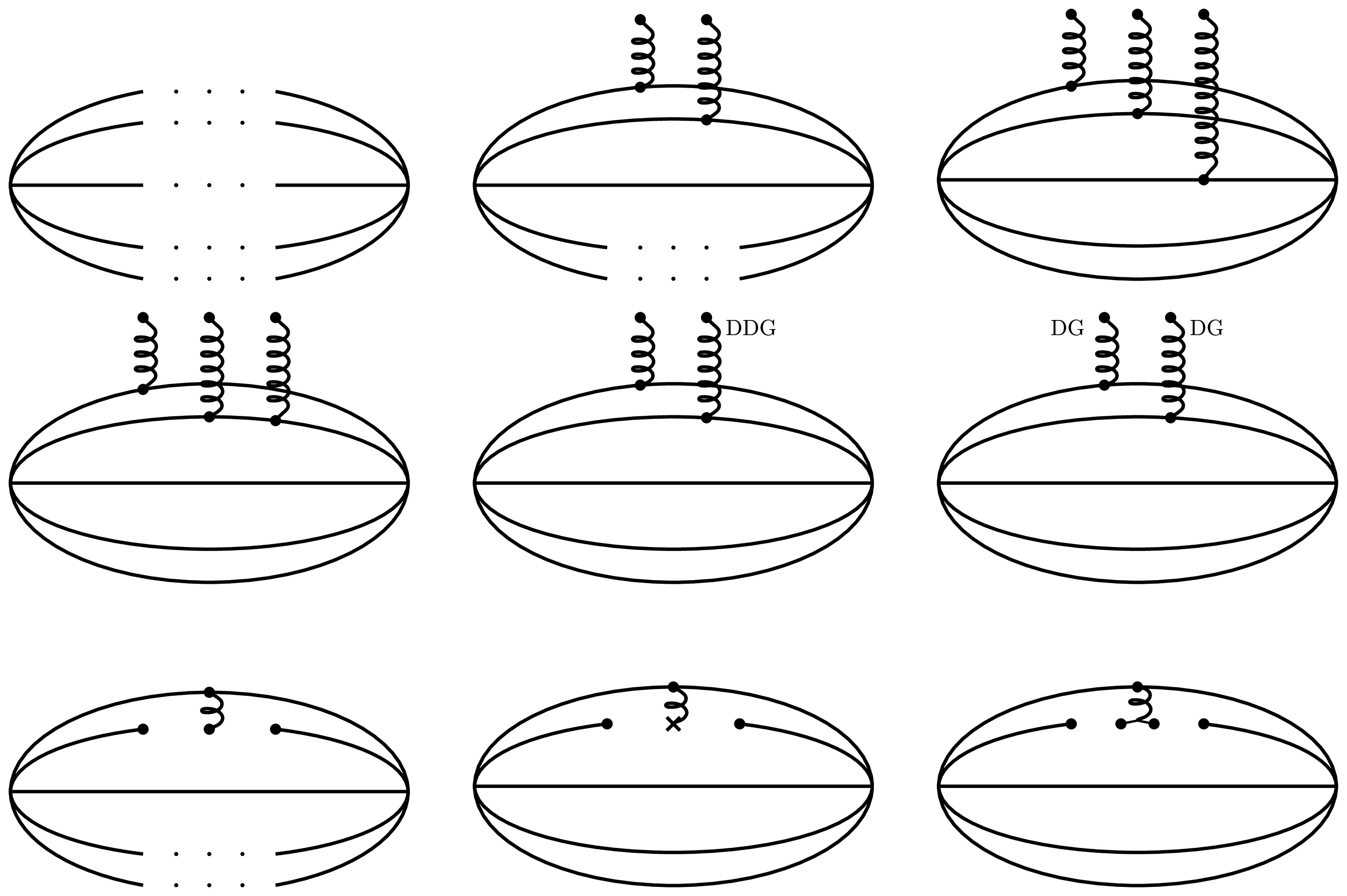
Figure 1. The Feynman diagrams involved in our calculations for the
$ \Xi(1530)\bar{K} $ molecular pentaquark state are shown. A quark line with dots represents terms proportional to the color factor$ \delta^{ij} $ in the propagator$ S^{ij}(x) $ ; consequently, such diagrams effectively subsume multiple Feynman diagrams.According to the principle of quark-hadron duality, the correlation function computed at the quark-gluon level is expected to be equivalent to that at the hadronic level. The Borel transform is then performed to suppress contributions from highly excited states. The hadron masses and coupling constants are obtained as
$ m_{\mp}^{2}(s_{0},M_{B}^2) =\:\frac{\int_{s_{<}}^{s_{0}}[\sqrt{s}\rho_{\not{p}}^{\text{OPE}}(s)\pm\rho_{I}^{\text{OPE}}(s)]s\; \mathrm{e}^{-s/M_{B}^{2}}\mathrm{d}s}{\int_{s_{<}}^{s_{0}}[\sqrt{s}\rho_{\not{p}}^{\text{OPE}}(s)\pm\rho_{I}^{\text{OPE}}(s)]\; \mathrm{e}^{-s/M_{B}^{2}}\mathrm{d}s} $
(16) and
$ f_{\mp}^{2}(s_{0},M_{B}) =\:\frac{\int_{s_<}^{s_{0}}[\sqrt{s}\rho_{\not{p}}^{\text{OPE}}(s)\pm\rho_{I}^{\text{OPE}}(s)]\mathrm{e}^{-s/M_{B}^{2}}\mathrm{d}s}{2m_{\mp}}\times \mathrm{e}^{m_{\mp}^{2}/M_{B}^{2}}\, , $
(17) which are functions of the Borel parameter
$ M_B $ and the continuum threshold$ s_0 $ .In the following analysis, we employ the same two-point QCD sum rule approach to determine the ground-state Ξ baryon mass and the corresponding coupling constant
$ f_{\Xi} $ that appears in Eq. (20). -
In QCD sum rules, the three-point correlation function is used to investigate the strong decay properties of hadrons. It is defined as
$ \begin{aligned}[b] \Pi_{\mu}(p_1^2,p_2^2,p^2)\equiv\;& \int \mathrm{d}^d x \mathrm{d}^d y \; \mathrm{e}^{\mathrm{i}p_1\cdot x}\mathrm{e}^{\mathrm{i}p_2\cdot y}\Gamma(x,y)\, ,\\ \Gamma(x,y)\equiv\;&\langle0|T[J_{\Xi}(x)J_{\bar{K}}(y)\bar{J}_{\mu}(0)]|0\rangle\, , \end{aligned} $
(18) where
$ J_{\Xi} $ denotes the interpolating current associated with the Ξ baryon$ J_{\Xi}(x) =\epsilon ^{abc}\left[ s^{aT}( x) C\gamma _{\mu } s^{b}( x)\right] \gamma ^{\mu } \gamma ^{5} q^{c}( x)\, . $
(19) The currents
$ J_{\Xi} $ and$ J_{\bar{K}} $ couple to the physical states$ |\Xi;1/2^+\rangle $ and$ |\bar{K};0^-\rangle $ , respectively, through the following matrix elements:$ \begin{aligned}[b]& \langle0|J_{\Xi}|\Xi;1/2^+\rangle=f_{\Xi}u(p_1)\, ,\\& \langle0|J_{\bar{K}}|\bar{K};0^-\rangle=\frac{f_{\bar{K}}m_{\bar{K}}}{m_s+m_d}\equiv \lambda_{\bar{K}}\, . \end{aligned} $
(20) The interactions among the
$ \Omega^* $ , Ξ, and$ \bar{K} $ hadrons are described by the effective Lagrangian [84]$ {\cal{L}}_{K \Xi\Omega^*}=\mathrm{i}g_{\Omega^*\Xi \bar{K}}\overline{\Xi}\gamma'^{\mu\nu\lambda}\gamma^5\left(\partial_\mu\Omega^*_\nu\right)\partial_\lambda \bar{K}+h.c.\, , $
(21) where
$ \gamma'^{\mu\nu\lambda}=i\varepsilon^{\mu\nu\lambda\alpha}\gamma_\alpha\gamma_5 $ .After inserting a complete set of intermediate hadronic states, the phenomenological representation of the three-point correlation function can be written as
$\begin{aligned}[b]& \Pi _{\mu}(p_1^2,p_2^2,p^2)\\=\;& \frac{\lambda_{\bar{K}}f_{\Xi}u(p_1)\langle \bar{K}(p_2)\Xi(p_1) | \Omega^*(p)\rangle f_-\bar{u}_\mu(p)}{(p^2-m_{\Omega^*}^{2}+\mathrm{i}\varepsilon)(p_1^2-m_\Xi^2+\mathrm{i}\varepsilon)(p_2^2-m_{\bar{K}}^2+\mathrm{i}\varepsilon)} +...\, ,\end{aligned} $
(22) where the “...” denotes the contributions of higher excited states, including those from opposite-parity states. After the Borel transformation, the ground-state contributions are expected to dominate the sum rules. Since both
$ \Omega^*(3/2^-) $ and$ \Xi(1/2^+) $ are treated as ground states in their corresponding channels, contamination from opposite-parity states is therefore suppressed and is not expected to significantly affect the numerical results. The transition matrix element can be derived from the effective Lagrangian in Eq. (21) as$ \langle \bar{K}(p_2)\Xi(p_1) |{\Omega^*}(p)\rangle=\bar{u}(p_1)\mathrm{i}g_{{\Omega^*}\Xi \bar{K}}\gamma'^{\mu\nu\lambda}\gamma^5p_2^{\lambda}p^{\mu}u_{\nu}(p)\, . $
(23) By substituting Eq. (23) into Eq. (22), we obtain
$ \begin{aligned}[b] \Pi _{\mu}(p_1^2,p_2^2,p^2) =\;& \frac{\mathrm{i}g_{{\Omega^*}\Xi \bar{K}}\lambda_{\bar{K}}f_{\Xi}f_-m_\Xi p_2 ^2 \not{p}_1\gamma^\mu\gamma^5}{3(p^2-m_{\Omega^*}^2+\mathrm{i}\epsilon)(p_1^2-m_\Xi^2+\mathrm{i}\varepsilon)(p_2^2-m_{\bar{K}}^2+\mathrm{i}\varepsilon)}\\& +...\, .\end{aligned} $
(24) Given the complexity of the full expression, we retain only the Lorentz structure
$ \not{p}_1 \gamma^{\mu}\gamma^{5} $ in Eq. (24) for the convenience of the subsequent analysis.This result can equivalently be rewritten as
$ \begin{aligned}[b]&\Pi _{\mu}(p_1^2,p_2^2,p^2) \\= \;& x\left(1+\frac{m^2_{\bar{K}}}{p_2^2-m_{\bar{K}}^2+\mathrm{i}\varepsilon}\right)\frac{\dfrac{1}{3}m_\Xi \mathrm{i}g_{{\Omega^*}\Xi \bar{K}}\lambda_{\bar{K}}f_{\Xi}f_-}{(p^2-m_{\Omega^*}^2+\mathrm{i}\varepsilon)(p_1^2-m_\Xi^2+\mathrm{i}\varepsilon)}\\& +...\, . \end{aligned} $
(25) Since
$ p = p_1 + p_2 $ , we consider the soft-kaon limit$ p_2 \to 0 $ , in which case$ p^2 \approx p_1^2 $ . In this limit, the terms proportional to$ 1/p_2^2 $ become dominant in the OPE series. Therefore, to properly construct the sum rules, we isolate the contributions with the Lorentz structure$ \not{p}_1 \gamma^\mu \gamma^5 $ proportional to$ 1/p_2^2 $ . This approximation has been examined in Ref. [85], where the results obtained in the soft-meson limit were found to be consistent with those obtained by treating the meson momentum as a small but finite quantity. This procedure determines the coupling constant$ g_{{\Omega^*}{\Xi}{\bar{K}}}(Q^2) $ (where$ Q^2 = -p_2^2 $ ) in a region away from the physical pole at$ Q^2 = -m_{\bar{K}}^2 $ . The on-shell coupling is then obtained by extrapolating from the valid QCD sum-rule window. By equating the hadronic and OPE representations, we obtain$ \begin{aligned}[b]&\frac{m^2_{\bar{K}}}{(p_2^2-m_{\bar{K}}^2+\mathrm{i}\varepsilon)}\frac{\dfrac{1}{3}m_\Xi \mathrm{i}g_{{\Omega^*}{\Xi}{\bar{K}}}\lambda_{\bar{K}}f_{\Xi}f_-}{(p^2-m_{\Omega^*}^2+\mathrm{i}\varepsilon)(p^2-m_\Xi^2+\mathrm{i}\varepsilon)}+...\\ =\;&\dfrac{1}{p^2_2}\left[\int_{0}^{s_0}\mathrm{d}s\frac{\rho(s)}{s-p^2}+\int_{s_0}^{\infty}\mathrm{d}s\frac{\rho(s)}{s-p^2}\right]\, . \end{aligned} $
(26) According to quark-hadron duality, the contributions of higher resonances and the continuum on the phenomenological side are assumed to be dual to the integral over the region above the continuum threshold
$ s_0 $ on the OPE side. After performing the Borel transform, the sum rules are obtained as$ \begin{aligned}[b]&\dfrac{1}{3}m_\Xi m^2_{\bar{K}} \mathrm{i}g_{{\Omega^*}{\Xi}{\bar{K}}}\lambda_{\bar{K}}f_{\Xi}f_- \frac{Q^2+m^2_{\bar{K}}}{Q^2}\frac{\mathrm{e}^{-m_{{\Omega^*}}^2/M^2_B}-\mathrm{e}^{-m_{\Xi}^2/M^2_B}}{m_{{\Omega^*}}^2-m_{\Xi}^2}\\ =\;&\int_{0}^{s_0}\mathrm{d}s\rho(s)\mathrm{e}^{-s/M^2_B}\, . \end{aligned}$
(27) To extract the value of the coupling constant at the physical point
$ Q^2 = -m_{\bar{K}}^2 $ , we extrapolate$ g_{{\Omega^*}{\Xi}{\bar{K}}}(Q^2) $ from the working region of the QCD sum rules using an exponential model [86−88]$ g_{{\Omega^*}{\Xi}{\bar{K}}}(Q^2)=g_1\mathrm{e}^{-g_2Q^2}\, , $
(28) where the parameters
$ g_1 $ and$ g_2 $ are determined by fitting the numerical results obtained from the sum rules.The decay width for the process
$ \Omega^*\rightarrow {\Xi}{\bar{K}} $ can be derived from Eq. (21) as$ \begin{aligned}[b]\Gamma(\Omega^*\rightarrow {\Xi}{\bar{K}}) =\;& \frac{\sqrt{\lambda(m_{{\Omega^*}}^2,m_{\Xi}^2,m_{\bar{K}}^2)}}{192\pi m_{{\Omega^*}}^3}g^2_{{\Omega^*}{\Xi}{\bar{K}}}\\& \times (m_{{\Omega^*}}^2-2m_{{\Omega^*}}m_{\Xi}-m_{\bar{K}}^2+m_{\Xi}^2)^2\\ &\times (m_{{\Omega^*}}^2+2m_{{\Omega^*}}m_{\bar{K}}-m_{\bar{K}}^2+m_{\Xi}^2)\, , \end{aligned} $
(29) where λ denotes the well-known Källén function
$ \lambda(a,b,c)=a^2+b^2+c^2-2ab-2ac-2bc\, . $
(30) At the quark–gluon level, we evaluate the three-point correlation function using the same light-quark propagators as those given in Eq. (14). We retain the spectral function
$ \rho^{\text{OPE}}(s) $ up to dimension 10, and the corresponding Feynman diagrams are shown in Fig. 2. The result for$ \rho(s) $ is obtained as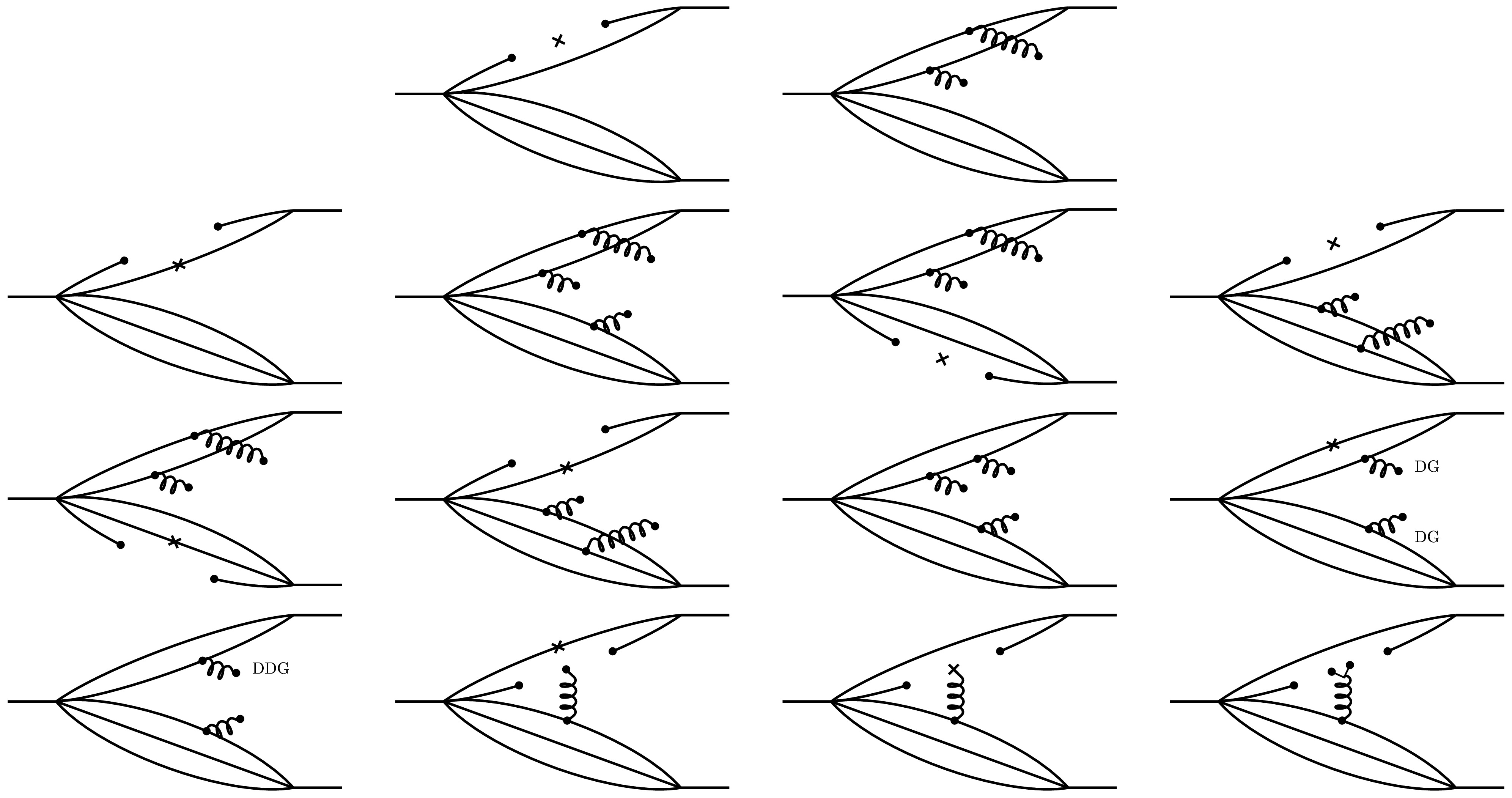
Figure 2. The Feynman diagrams that contribute to the theoretical side of the three-point sum rules in the relevant structure for the two-body strong decays of the
$ \Xi(1530)\bar{K} $ molecular pentaquark state are shown.$ \begin{aligned}[b] \rho^{\text{OPE}}(s)=\;& \frac{5\langle g^{2}G^{2}\rangle}{98304\pi^{6}}s^{2}+\frac{5m_{s}\langle\overline{s}s\rangle}{6144\pi^{4}}s^{2}-\frac{5m_{s}\langle\overline{q}q\rangle}{3072\pi^{4}}s^{2}\\&- \frac{7 g^{2}\langle\overline{s}s\rangle^{2}}{41472\pi^{4}}s-\frac{7 g^{2}\langle\overline{q}q\rangle^{2}}{41472\pi^{4}}s-\frac{7 \langle g^3fG^{3}\rangle}{2^{15}\times3^3\times\pi^{6}}s\\ & - \frac{7 m_{s}\langle \bar{s}g\sigma Gs\rangle}{18432\pi^{4}}s+\frac{m_{s}\langle \bar{q}g\sigma Gq\rangle}{1536\pi^{4}}s\\ & - \frac{55m_{s}\langle\overline{s}s\rangle\langle g^{2}G^{2}\rangle}{12288\pi^{4}}+\frac{5m_{s}\langle\bar{q}q\rangle\langle g^{2}G^{2}\rangle}{6144\pi^{4}}\, . \end{aligned} $
(31) -
For the numerical analyses, we adopt the values of the QCD parameters at the renormalization scale
$ \mu = 1\; \mathrm{GeV} $ and set$ \Lambda_{\rm QCD}=300\; \mathrm{MeV} $ , as is standard in QCD sum rule calculations [42, 80, 89−96]$ \begin{aligned}[b] m_u =\;&m_d=0\, ,m_s=93.5\pm0.8\; \mathrm{MeV}\, ,\\ \langle\bar{q}q\rangle =\;&-(0.24\pm0.01)^3\; \mathrm{GeV^3}\, ,\\ \langle\bar{s}s\rangle =\;&(0.8\pm 0.1)\langle\bar{q}q\rangle\, ,\\ \langle\bar{q}g\sigma Gq\rangle =\;&(0.8\pm 0.2)\langle\bar{q}q\rangle \; \mathrm{GeV^2}\, ,\\ \langle g^2 G^2 \rangle =\;&(0.48\pm 0.14) \; \mathrm{GeV^4}\, ,\\ \langle g^3fG^3 \rangle =\;&(8.2\pm 1)\langle \alpha_s G^2 \rangle\; \mathrm{GeV^2}\, . \end{aligned} $
(32) Here, the strange quark mass is evaluated at the renormalization scale
$ \mu = 2\; \mathrm{GeV} $ . The renormalization group equation is used to evolve$ m_s $ to the working scale$ \mu = 1\; \mathrm{GeV} $ .We begin by examining the behavior of the spectral function before proceeding to the mass sum rule analysis. As illustrated in Fig. 3, the spectral density exhibits poor positivity, becoming negative over a relatively wide region,
$ 1\; \mathrm{GeV}^2 \leq s \leq 4\; \mathrm{GeV}^2 $ . To remedy this unphysical behavior, we relax the factorization assumption by introducing a parameter κ via$ \langle\bar{q}\bar{q}qq\rangle=\kappa\langle\bar{q}q\rangle^2 $ [96−98]. With$ \kappa=3.90 $ , the spectral density exhibits sufficiently good behavior; this value is adopted in the following analysis. The associated uncertainty is estimated by varying κ within$ \kappa = 3.90 \pm 0.30 $ and is included in the final error estimates.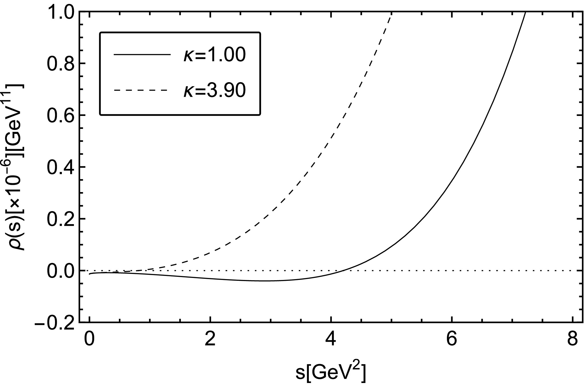
Figure 3. Behavior of the spectral densities under different factorization assumptions. The solid lines represent the spectral densities for
$ \kappa=1 $ , whereas the dashed lines show the corresponding densities for$ \kappa=3.90 $ .In Eq. (16), the extracted hadron mass depends on two free parameters: the Borel parameter
$ M_B^2 $ and the continuum threshold$ s_0 $ . Their working regions are determined by imposing the following standard criteria: (a) good convergence of the operator product expansion, (b) a sufficiently large pole contribution, and (c) good stability of the mass sum rules.The convergence of the OPE is quantified by requiring that the contributions from high-dimensional operators be sufficiently suppressed
$ \mathrm{CVG}\equiv\left|\frac{\Pi_-^{12+13}(\infty,M_B^2)}{\Pi_-(\infty,M_B^2)}\right|\leq5{\text{%}}\, , $
(33) where
$ \Pi_- $ denotes the full OPE series of the correlation function, while$ \Pi_-^{12+13} $ represents the combined contributions from the dimension-12 and dimension-13 condensates. As shown in Fig. 4, this requirement leads to a lower bound on the Borel parameter,$ M_B^2 \geq 1.25\; \mathrm{GeV}^2 $ .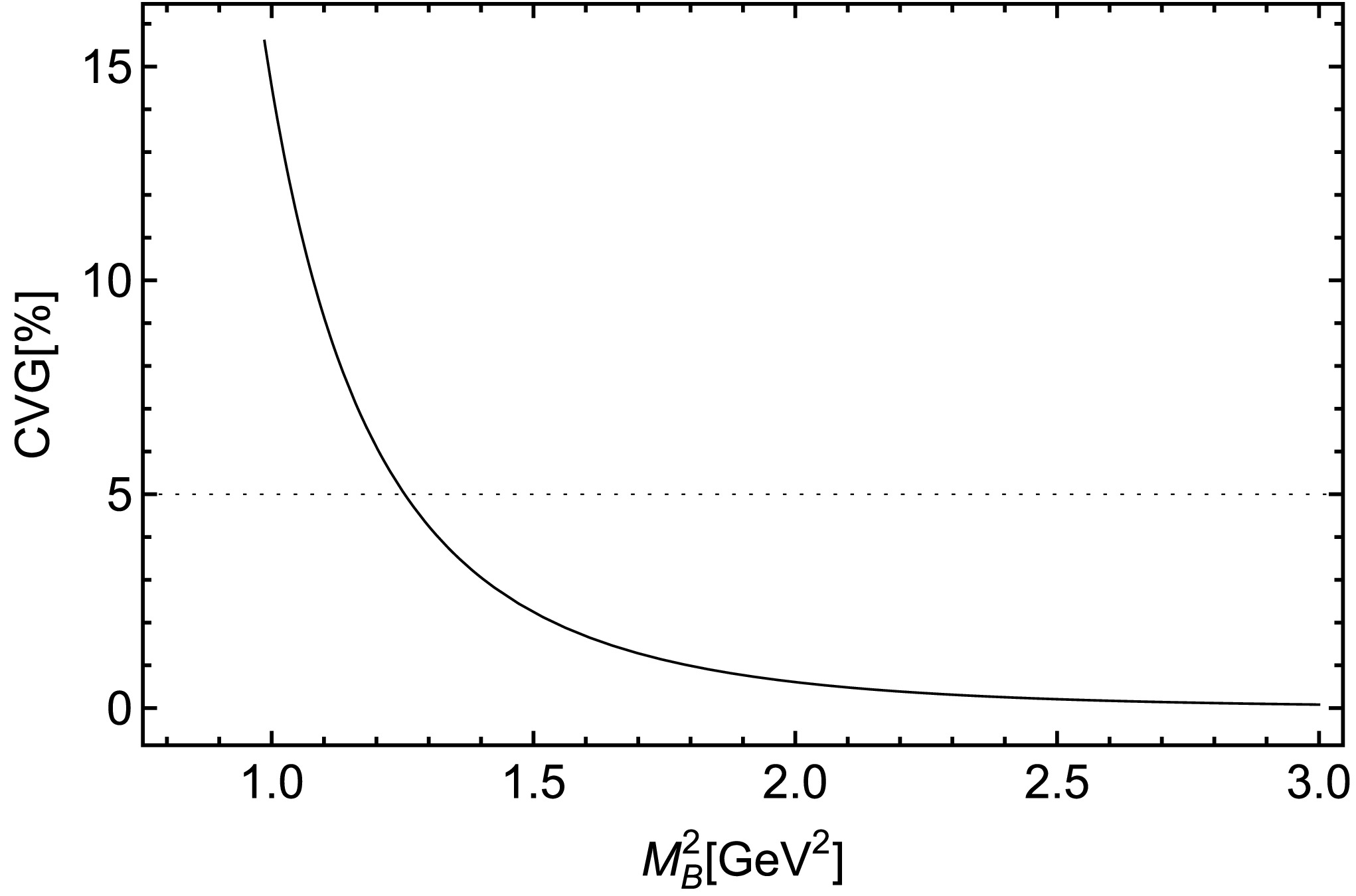
Figure 4. OPE convergence for the
$ \Xi(1530)\bar{K} $ molecular pentaquark state at$ \kappa=3.90 $ .To determine the optimal value of the continuum threshold
$ s_0 $ , we plot the$ m_H $ –$ s_0 $ curves for different values of$ M_B^2 $ in Fig. 5. The optimal$ s_0 $ is chosen such that the dependence of$ m_H $ on$ M_B^2 $ is minimized in its vicinity. To quantify this criterion, we define the function$ \chi^2 $ as [99−102]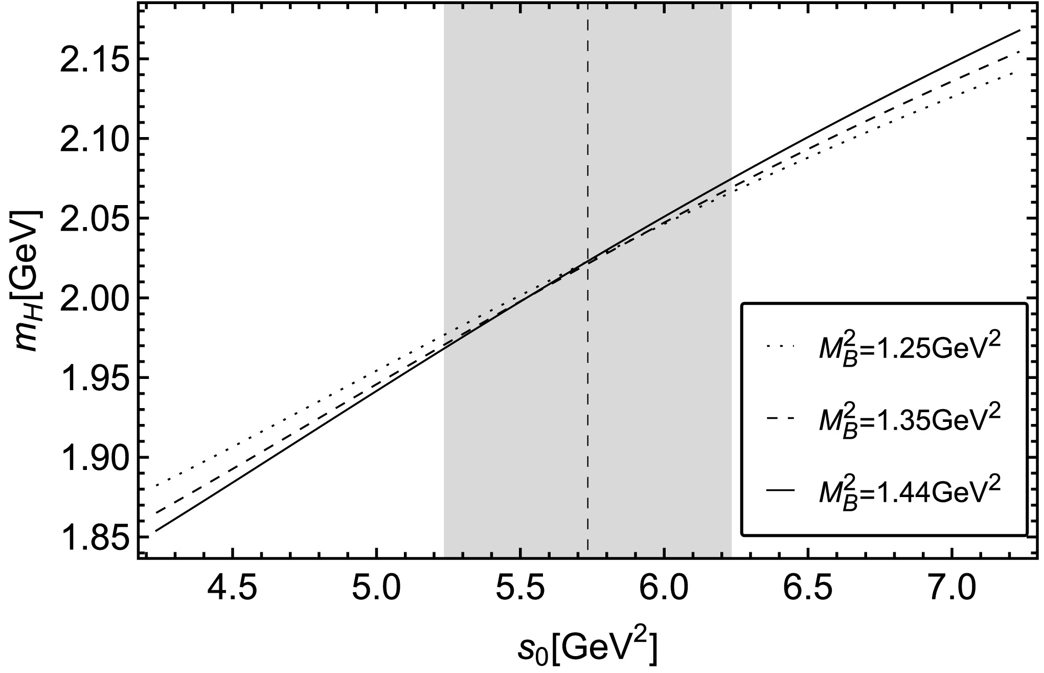
Figure 5. Variation of the hadron mass with
$ s_0 $ for the$ \Xi(1530)\bar{K} $ molecular pentaquark state, considering$ \kappa=3.90 $ .$ \chi^2(s_0)=\sum\limits_{i=1}^{N}\left[\frac{m_H(s_0,M^2_{B,i})}{\bar{m}_H(s_0)}-1\right]^2\, , $
(34) where
$ \bar{m}_H(s_0) $ denotes the average of the data points$ \bar{m}_H(s_0)=\sum\limits_{i=1}^{N}\frac{m_H(s_0,M^2_{B,i})}{N}\, . $
(35) The
$ \chi^2 $ as a function of$ s_0 $ is shown in Fig. 6, from which the optimal value of the continuum threshold is determined by the location of the minimum, yielding$ s_0=5.73 $ GeV2.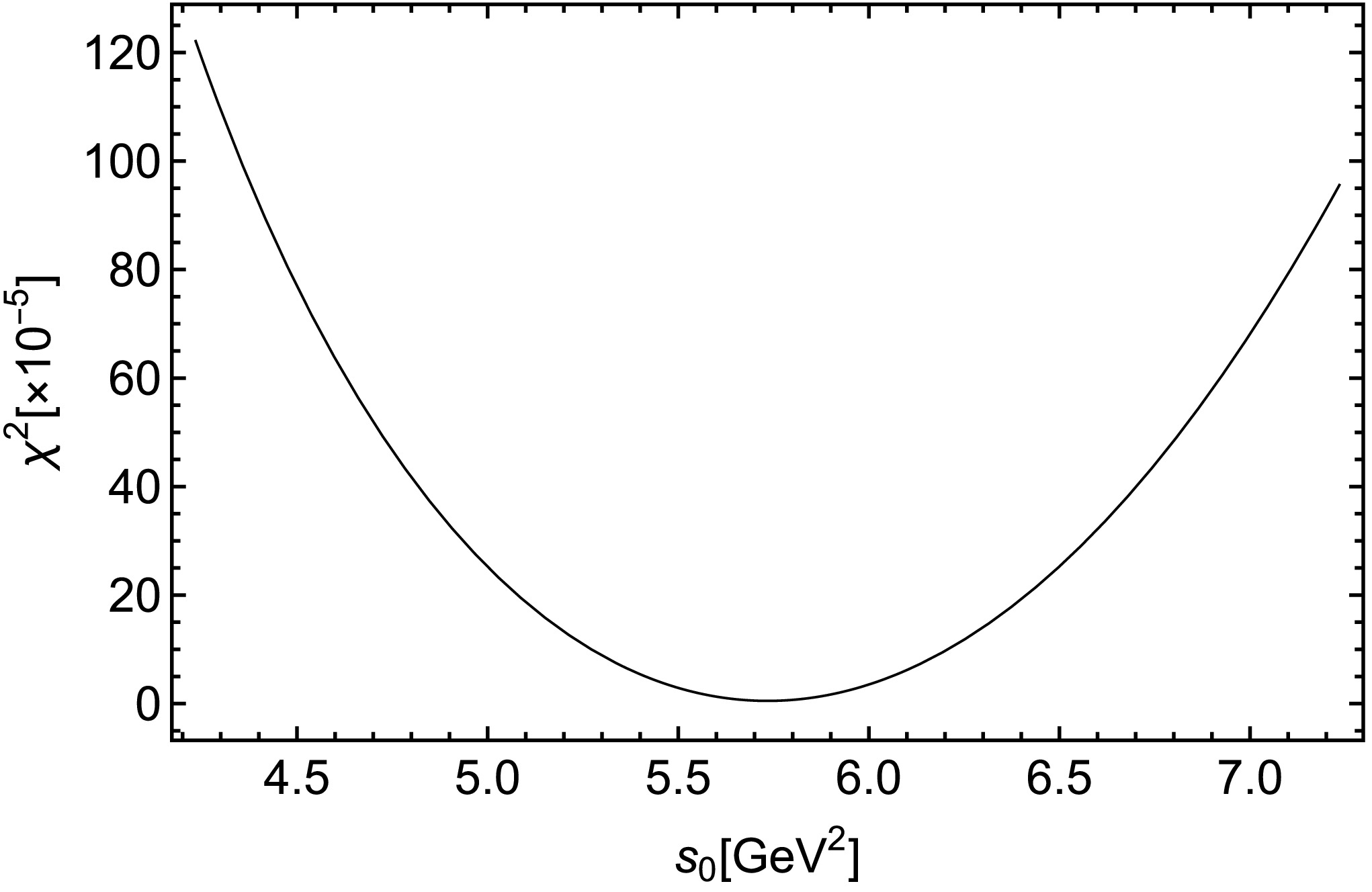
Figure 6. Variation of
$ \chi^2 $ with$ s_0 $ for the$ \Xi(1530)\bar{K} $ molecular pentaquark state, with$ \kappa=3.90 $ .In addition, to ensure a sufficient pole contribution, we require
$ \mathrm{PC}\equiv\left|\frac{\Pi_-(s_0,M_B^2)}{\Pi_-(\infty,M_B^2)}\right|\geq50{\text{%}}\, . $
(36) Applying the above constraints yields an acceptable Borel window of
$ 1.25\; \mathrm{GeV}^2 \leq M_B^2 \leq 1.44\; \mathrm{GeV}^2 $ . The corresponding Borel curves are displayed in Fig. 7, where the extracted mass exhibits good stability with respect to variations in$ M_B^2 $ within this window. As a result, we obtain the mass and coupling constant of the$ \Xi(1530)\bar{K} $ molecular state as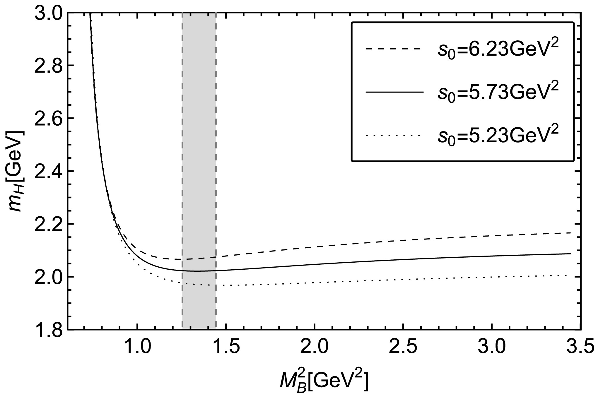
Figure 7. Variation of the hadron mass with
$ M^2_B $ for the$ \Xi(1530)\bar{K} $ molecular pentaquark state, considering$ \kappa=3.90 $ .$ m_{\Xi(1530)K}=2.02\pm0.12\; \mathrm{GeV}\, , $
(37) $ f_-=(4.60\pm1.17)\times10^{-4}\; \mathrm{GeV}^6\, , $
(38) where the errors mainly arise from the uncertainties in the various condensates in Eq. (32), as well as from the phenomenological parameter κ. The extracted mass of the
$ \Xi(1530)\bar{K} $ molecular pentaquark state is consistent with the mass of$ \Omega(2012) $ reported by the PDG [42]. -
To calculate the coupling constant of Ξ, we perform a mass sum rule analysis for the current in Eq. (19) and adopt the same values for the QCD parameters as those in Eq. (32). Under the following constraints
$ \begin{aligned}[b] \mathrm{CVG}\equiv\;&\left|\frac{\Pi_-^{6+7+8}(\infty,M_B^2)}{\Pi_-(\infty,M_B^2)}\right|\leq10{\text{%}}\, ,\\\mathrm{PC}\equiv\;&\left|\frac{\Pi_-(s_0,M_B^2)}{\Pi_-(\infty,M_B^2)}\right|\geq40{\text{%}}\, , \end{aligned} $
(39) the acceptable Borel window is determined to be
$ 1.01\; \mathrm{GeV}^2 \leq M_B^2 \leq 1.20\; \mathrm{GeV}^2 $ . The corresponding Borel curves are shown in Fig. 8. As a result, we obtain the mass and coupling constant of the Ξ baryon as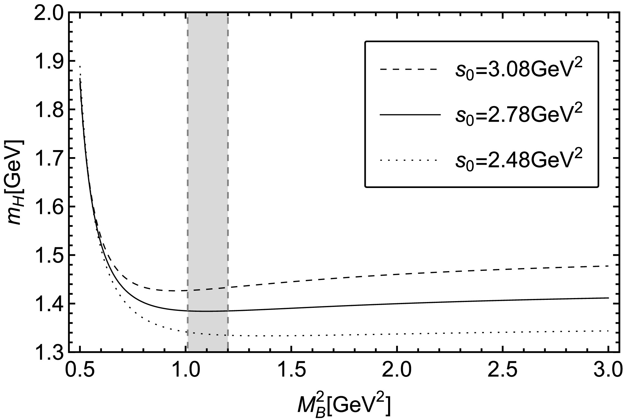
Figure 8. Variation of the hadron mass with
$ M^2_B $ for the Ξ state.$ m_{\Xi}=1.38\pm0.06\; \mathrm{GeV}\, , $
(40) $ f_{\Xi}=(3.21\pm0.39)\times10^{-2}\; \mathrm{GeV^3}\, , $
(41) where the obtained mass agrees well with the mass of the Ξ baryon with
$ J^P=1/2^+ $ listed in the PDG [42]. -
To perform the three-point sum rule analyses, we adopt the input parameters listed in Eq. (32) and use the same factorization parameter,
$ \kappa=3.90 $ . For the Ξ and$ \bar{K} $ doublets, as well as$ \Omega(2012) $ , we use the hadronic parameter values from the PDG [42]:$ \begin{aligned}[b] m_{\Omega(2012)} =\;&2012.4\pm0.9\; \mathrm{MeV}\, ,\\ m_{\Xi^-} =\;&1321.71\pm0.07\; \mathrm{MeV}\, , \\ m_{\Xi^0} =\;&1314.86\pm0.20\; \mathrm{MeV}\, , \\m_{\bar{K}^0} =\;&497.611\pm0.013\; \mathrm{MeV}\, , \\ m_{K^-} =\;&493.677\pm0.015\; \mathrm{MeV}\, , \\ f_{\bar{K}} =\;&155.7\; \mathrm{MeV}\, . \end{aligned} $
(42) As shown in Eq. (27), the coupling constant extracted from the sum rule depends on
$ s_0 $ and$ M_B^2 $ in the limit$ Q^2 \to 0 $ . Adopting the same value,$ s_0=5.73 $ GeV2, as in the mass sum rule, we present the dependence of the coupling constant on$ M^2_B $ at the Euclidean momentum point$ Q^2 = m^2_{\Xi^-} $ in Fig. 9. We find that the sum rules yield a stable plateau for the coupling constant at$ M_B^2= 0.71\; \mathrm{GeV^2} $ , around which it exhibits minimal parameter dependence.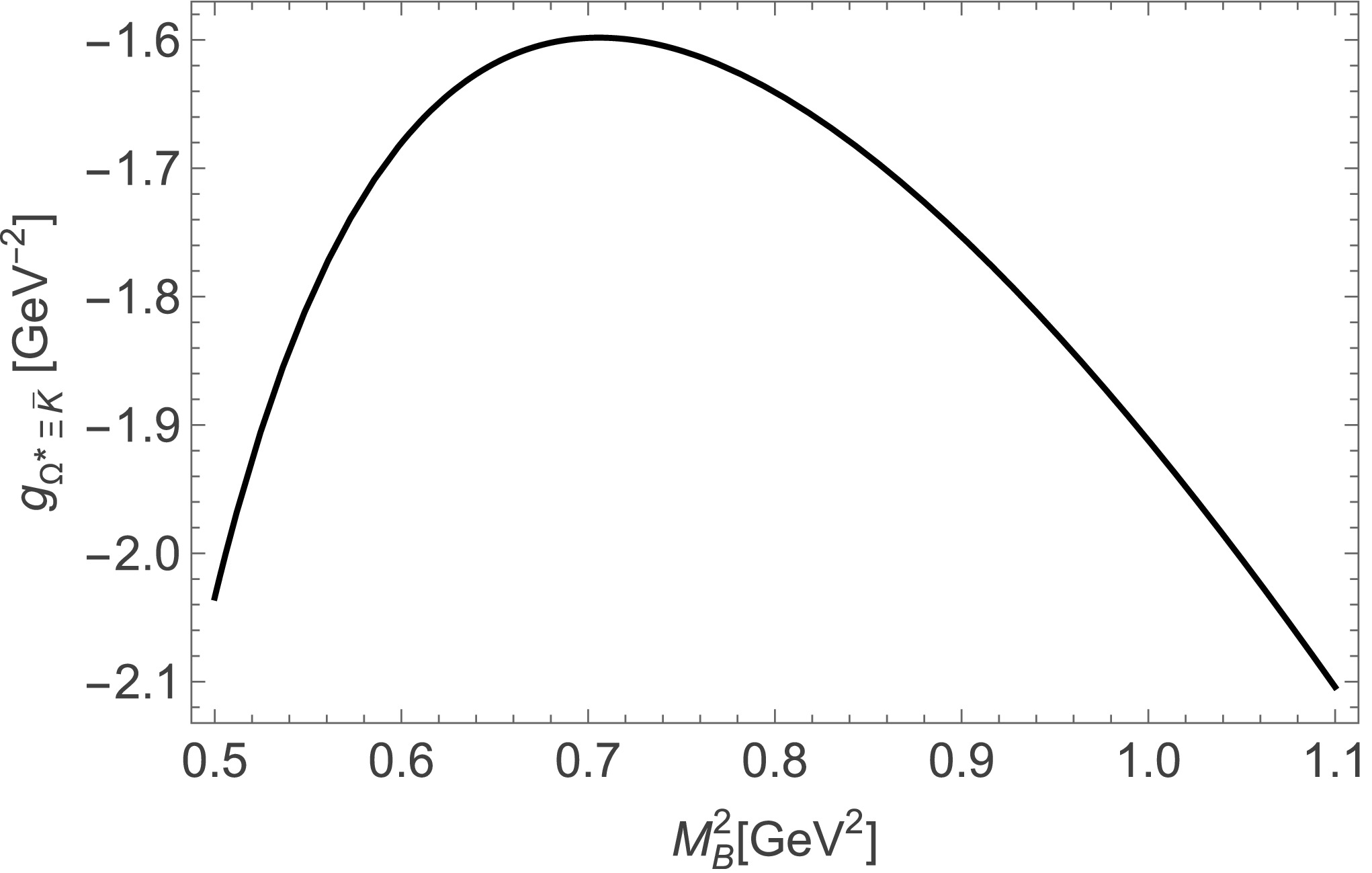
Figure 9. Dependence of the coupling constant
$ g_{{\Omega^*}\Xi^- \bar{K}^0}(Q^2 = $ $ m^2_{\Xi^-}) $ on the Borel parameter$ M_B^2 $ for$ s_0=5.73 $ GeV2.To extract the value of the coupling constant at the physical point
$ Q^2 = -m_{\bar{K}^0}^2 $ , we extrapolate$ g_{{\Omega^*}\Xi^- \bar{K}^0}(Q^2) $ from the QCD sum-rule working region using the exponential model given in Eq. (28). As shown in Fig. 10, the QCD sum-rule results obtained with$ s_0=5.73\; \mathrm{GeV}^2 $ and$ M_B^2=0.71\; \mathrm{GeV}^2 $ are well described by this model, yielding the fitted parameters$ g_1=-1.82\; \mathrm{GeV}^{-2} $ and$ g_2=0.07\; \mathrm{GeV}^{-2} $ . Using these parameters, the coupling constant at$ Q^2=-m_{\bar{K}^0}^2 $ is obtained as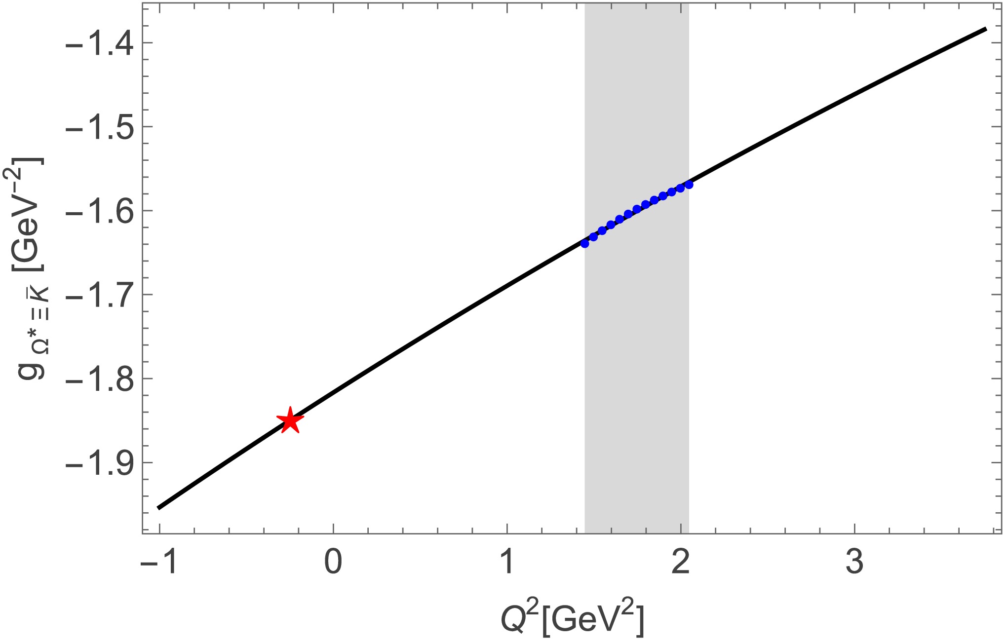
Figure 10. Variation of the coupling constant
$ g_{{\Omega^*}\Xi^- \bar{K}^0} $ with$ Q^2 $ . The dotted points represent the QCD sum-rule results for$ g_{{\Omega^*}\Xi^- \bar{K}^0} $ at$ s_0=5.73\; \mathrm{GeV^2} $ and$ M_B^2=0.71\; \mathrm{GeV^2} $ . The solid line shows the fit to the QCD sum-rule results using the model in Eq. (28), extrapolated to the physical pole$ Q^2=-m_{\bar{K}^0}^2 $ .$ g_{{\Omega^*}\Xi^- \bar{K}^0}=-1.85^{+0.87}_{-0.69}\; \mathrm{GeV}^{-2}\, , $
(43) where the errors mainly arise from the uncertainties in the coupling constants in Eqs. (38) and (41), the various condensates in Eq. (32), the hadronic parameter values in Eq. (42), and the phenomenological parameter κ.
Using Eq. (29), the partial decay width of the process
$ \Omega(2012)\rightarrow \Xi^-\bar{K}^0 $ can be calculated as$ \Gamma({\Omega^*}\rightarrow \Xi^-\bar{K}^0)=0.44^{+0.51}_{-0.27}\; \mathrm{MeV}\, . $
(44) For the
$ \Omega(2012)\rightarrow \Xi^0K^- $ decay, the dominant difference arises from the isospin mass splitting of the Ξ and$ \bar{K} $ doublets in the final state. Possible isospin-breaking effects in the interpolating current and the OPE, such as those induced by$ m_u \neq m_d $ , are neglected because of their small numerical impact. Following the same procedure, we obtain the fitted parameters$ g_1 = 1.85\; \mathrm{GeV}^{-2} $ and$ g_2 = 0.07\; \mathrm{GeV}^{-2} $ in the extrapolation model. With these values, the coupling constant at$ Q^2 = -m_{K^-}^2 $ and the corresponding partial decay width are determined to be$ g_{{\Omega^*}\Xi^0 K^-}=1.88^{+0.88}_{-0.70}\; \mathrm{GeV}^{-2}\, , $
(45) $ \Gamma({\Omega^*}\rightarrow \Xi^0K^-)=0.52^{+0.60}_{-0.31}\; \mathrm{MeV}\, . $
(46) As a result, the total two-body decay width of the
$ \Xi^\ast \bar{K} $ molecular pentaquark state is$ \Gamma({\Omega^*}\rightarrow \Xi \bar{K})=0.96^{+0.79}_{-0.41}\; \mathrm{MeV}\, . $
(47) This value agrees with the theoretical predictions of the effective Lagrangian approach in Refs. [58, 61, 62]. Since three-body decays are neglected, it is also roughly consistent with the results reported by ALICE [39]. The branching-fraction ratio for the two-body decays is obtained as
$ {\cal{R}}^{\Xi^-\bar{K}^0}_{\Xi^0K^-}\equiv \frac{{\cal{B}}[\Omega(2012)\rightarrow \Xi^-\bar{K}^0]}{{\cal{B}}[\Omega(2012)\rightarrow \Xi^0K^-]} = \frac{\Gamma({\Omega^*}\rightarrow \Xi^-\bar{K}^0)}{\Gamma({\Omega^*}\rightarrow \Xi^0K^-)}\approx 0.85\, , $
(48) which agrees well with the experimental data compiled by the PDG [42].
-
In this work, we have investigated the recently observed
$ \Omega(2012) $ as a$ \Xi(1530)\bar{K} $ molecular pentaquark state within the framework of QCD sum rules. We construct the unique molecular interpolating current with$ I(J^P)=0(\dfrac{3}{2}^-) $ and calculate the correlation functions by employing parity-projected sum rules to separate the positive- and negative-parity contributions. We calculate the two-point correlation function to investigate the hadron mass and the three-point correlation function to study the two-body strong decay properties of the$ \Xi(1530)\bar{K} $ pentaquark state.Our QCD sum rule analyses yield a mass of
$ 2.02\pm0.12\; \mathrm{GeV} $ for the$ \Xi(1530)\bar{K} $ molecular pentaquark state and a total two-body decay width of$ \Gamma({\Omega^*} \rightarrow \Xi \bar{K}) = 0.96^{+0.79}_{-0.41}\; \mathrm{MeV} $ . The branching fraction ratio of the two-body decay channels is obtained as$ {\cal{R}}^{\Xi^-\bar{K}^0}_{\Xi^0K^-} = 0.85 $ . These results are in agreement with the experimental data for$ \Omega(2012) $ within uncertainties, supporting its interpretation as a$ \Xi(1530)\bar{K} $ molecular pentaquark state. These calculations are expected to provide further insight into the internal structure of$ \Omega(2012) $ in the future. -
The explicit expressions for the spectral densities
$ \rho_{\not{p}}^{\text{OPE}}(s) $ and$ \rho_{I}^{\text{OPE}}(s) $ are presented in Eqs. (A1) and (A2), respectively.$ \begin{aligned}[b] \rho_{\not{p}}^{\text{OPE}}(s)=\;& \frac{ s^5}{15728640 \pi ^8}+\frac{31 \langle\bar{s}s\rangle m_s s^3}{737280 \pi ^6}-\frac{13 \langle\bar{q}q\rangle m_s s^3}{92160 \pi ^6}+\frac{61 \langle g^{2}G^{2}\rangle s^3}{212336640 \pi ^8}+\frac{251 \langle\bar{q}g\sigma Gq\rangle m_s s^2}{368640 \pi ^6}+ \frac{ \langle\bar{s}g\sigma Gs\rangle m_s s^2}{6144 \pi ^6}-\frac{ g^{2} \langle\bar{q}q\rangle^2 s^2}{41472 \pi ^6}\\&-\frac{83 g^{2} \langle\bar{s}s\rangle^2 s^2}{622080 \pi ^6}-\frac{\langle\bar{q}q\rangle^2 s^2}{4608 \pi ^4}+\frac{7 \langle\bar{s}s\rangle^2 s^2}{11520 \pi ^4}+\frac{\langle\bar{q}q\rangle \langle\bar{s}s\rangle s^2}{360 \pi ^4} - \frac{23 \langle g^3G^{3}\rangle s^2}{5308416 \pi ^8}-\frac{35 \langle g^{2}G^{2}\rangle \langle\bar{q}q\rangle m_s s}{110592 \pi ^6}-\frac{329 \langle g^{2}G^{2}\rangle \langle\bar{s}s\rangle m_s s}{589824 \pi ^6}\\&+\frac{\langle\bar{q}q\rangle \langle\bar{q}g\sigma Gq\rangle s}{4608 \pi ^4} - \frac{37 \langle\bar{q}q\rangle \langle\bar{s}g\sigma Gs\rangle s}{4608 \pi ^4}-\frac{49 \langle\bar{s}s\rangle \langle\bar{q}g\sigma Gq\rangle s}{6912 \pi ^4}-\frac{143 \langle\bar{s}s\rangle \langle\bar{s}g\sigma Gs\rangle s}{27648 \pi ^4}-\frac{\langle\bar{q}q\rangle \langle\bar{s}g\sigma Gs\rangle m_s^2}{864 \pi ^4}\\ & - \frac{91 \langle\bar{s}s\rangle \langle\bar{s}g\sigma Gs\rangle m_s^2}{6912 \pi ^4}+\frac{2405 \langle g^{2}G^{2}\rangle \langle\bar{s}g\sigma Gs\rangle m_s}{5308416 \pi ^6}+\frac{985 \langle g^{2}G^{2}\rangle \langle\bar{q}g\sigma Gq\rangle m_s}{5308416 \pi ^6}+\frac{\langle\bar{s}s\rangle^3 m_s}{96 \pi ^2} - \frac{13 \langle\bar{q}q\rangle^2 \langle\bar{s}s\rangle m_s}{96 \pi ^2}\\&-\frac{5 g^{2} \langle\bar{q}q\rangle^2 \langle\bar{s}s\rangle m_s}{1152 \pi ^4}+\frac{5 g^{2} \langle\bar{q}q\rangle \langle\bar{s}s\rangle^2 m_s}{1296 \pi ^4}-\frac{11 g^{2} \langle\bar{s}s\rangle^3 m_s}{1944 \pi ^4} - \frac{ g^{2} \langle\bar{q}q\rangle^3 m_s}{2592 \pi ^4}+\frac{11 \langle g^3G^{3}\rangle \langle\bar{q}q\rangle m_s}{24576 \pi ^6}\\&+\frac{113 \langle g^3G^{3}\rangle \langle\bar{s}s\rangle m_s}{147456 \pi ^6}-\frac{11 g^{2} \langle g^{2}G^{2}\rangle \langle\bar{q}q\rangle^2 }{2239488 \pi ^6} - \frac{\langle g^{2}G^{2}\rangle \langle\bar{q}q\rangle^2 }{6912 \pi ^4}+\frac{11 \langle g^{2}G^{2}\rangle \langle\bar{s}s\rangle^2 }{9216 \pi ^4}+\frac{41 \langle g^{2}G^{2}\rangle \langle\bar{s}s\rangle^2 }{8957952 \pi ^6}\\& + \frac{11 \langle g^{2}G^{2}\rangle \langle\bar{q}q\rangle \langle\bar{s}s\rangle }{13824 \pi ^4}+\frac{193 \langle\bar{q}g\sigma Gq\rangle \langle\bar{s}g\sigma Gs\rangle}{27648 \pi ^4}+\frac{5 \langle\bar{q}g\sigma Gq\rangle^2}{27648 \pi ^4}+\frac{3 \langle\bar{s}g\sigma Gs\rangle^2}{1024 \pi ^4} - \frac{5 {\langle g^{2}G^{2}\rangle} {\langle\bar{q}q\rangle} {\langle\bar{q}g\sigma Gq\rangle} \delta (s)}{27648 \pi ^3}\\&-\frac{5 {g}^4 {\langle\bar{q}q\rangle}^2 {\langle\bar{s}s\rangle}^2\delta (s)}{139968 \pi ^3}-\frac{5 {g}^4 {\langle\bar{q}q\rangle}^4 \delta (s)}{839808 \pi ^3}-\frac{11 {g}^2 {\langle\bar{q}g\sigma Gq\rangle} {\langle\bar{s}s\rangle}^2 {m_s}\delta (s)}{20736 \pi ^3}- \frac{11 {g}^2 {\langle\bar{q}q\rangle}^2 {\langle\bar{q}g\sigma Gq\rangle} {m_s}\delta (s)}{31104 \pi ^3}\\ &-\frac{13 {g}^2 {\langle\bar{q}q\rangle}^2 {\langle\bar{s}g\sigma Gs\rangle} {m_s}\delta (s)}{31104 \pi ^3}-\frac{17 {g}^2 \langle g^3G^{3}\rangle {\langle\bar{q}q\rangle}^2 \delta (s)}{11943936 \pi ^5}- \frac{11 {g}^2 {\langle\bar{q}q\rangle} {\langle\bar{s}s\rangle}^3\delta (s)}{2916 \pi }-\frac{11 {g}^2 {\langle\bar{q}q\rangle}^3 {\langle\bar{s}s\rangle}\delta (s)}{5832 \pi }\\&-\frac{7 {g}^2 {\langle\bar{q}q\rangle}^2 {\langle\bar{s}s\rangle}^2\delta (s)}{11664 \pi } - \frac{13 {\langle\bar{q}q\rangle} {\langle\bar{q}g\sigma Gq\rangle} {\langle\bar{s}s\rangle} {m_s}\delta (s)}{96 \pi }-\frac{{\langle\bar{q}g\sigma Gq\rangle} {\langle\bar{s}s\rangle}^2 {m_s}\delta (s)}{288 \pi }-\frac{19 {\langle\bar{q}q\rangle}^2 {\langle\bar{s}g\sigma Gs\rangle} {m_s}\delta (s)}{288 \pi }\\& - \frac{17 {\langle\bar{q}q\rangle} {\langle\bar{s}s\rangle} {\langle\bar{s}g\sigma Gs\rangle} {m_s}\delta (s)}{864 \pi }+\frac{\langle g^3G^{3}\rangle {\langle\bar{q}q\rangle} {\langle\bar{s}s\rangle}\delta (s)}{9216 \pi ^3}-\frac{\langle g^3G^{3}\rangle {\langle\bar{q}q\rangle}^2 \delta (s)}{27648 \pi ^3} + \frac{\langle g^3G^{3}\rangle {\langle\bar{q}g\sigma Gq\rangle} {m_s}\delta (s)}{49152 \pi ^5}\\ &+\frac{133 {\langle g^{2}G^{2}\rangle}^2 {\langle\bar{s}s\rangle} {m_s}\delta (s)}{5308416 \pi ^5}+\frac{73 {\langle g^{2}G^{2}\rangle} {\langle\bar{s}s\rangle} {\langle\bar{s}g\sigma Gs\rangle}\delta (s)}{55296 \pi ^3} - \frac{5 {g}^4 {\langle\bar{s}s\rangle}^4\delta (s)}{279936 \pi ^3}-\frac{13 {g}^2 {\langle\bar{s}s\rangle}^2 {\langle\bar{s}g\sigma Gs\rangle} {m_s}\delta (s)}{124416 \pi ^3}\\&-\frac{31 {g}^2 \langle g^3G^{3}\rangle {\langle\bar{s}s\rangle}^2\delta (s)}{11943936 \pi ^5} - \frac{13 {g}^2 {\langle\bar{s}s\rangle}^4\delta (s)}{23328 \pi }+\frac{13 {\langle\bar{s}s\rangle}^2 {\langle\bar{s}g\sigma Gs\rangle} {m_s}\delta (s)}{864 \pi }-\frac{\langle g^3G^{3}\rangle {\langle\bar{s}s\rangle}^2\delta (s)}{13824 \pi ^3}-\frac{17 \langle g^3G^{3}\rangle {\langle\bar{s}g\sigma Gs\rangle} {m_s}\delta (s)}{1769472 \pi ^5}\, . \end{aligned} $
(A1) $ \begin{aligned}[b] \rho_{I}^{\text{OPE}}(s)=\;& \frac{3 m_s s^5}{5734400 \pi ^8}-\frac{\langle\bar{s}s\rangle s^4}{49152 \pi ^6}-\frac{\langle\bar{q}q\rangle s^4}{110592 \pi ^6}+\frac{7 \langle\bar{q}g\sigma Gq\rangle s^3}{92160 \pi ^6}+\frac{47 \langle\bar{s}g\sigma Gs\rangle s^3}{276480 \pi ^6} + \frac{79 \langle g^{2}G^{2}\rangle m_s s^3}{8847360 \pi ^8}+\frac{23 \langle\bar{s}g\sigma Gs\rangle m_s^2 s^2}{36864 \pi ^6}\\&+\frac{\langle\bar{q}q\rangle^2 m_s s^2}{768 \pi ^4}-\frac{\langle\bar{s}s\rangle^2 m_s s^2}{128 \pi ^4} + \frac{13 \langle\bar{q}q\rangle \langle\bar{s}s\rangle m_s s^2}{768 \pi ^4}+\frac{13 g^{2} \langle\bar{q}q\rangle^2 m_s s^2}{165888 \pi ^6}-\frac{7 g^{2} \langle\bar{s}s\rangle^2 m_s s^2}{995328 \pi ^6}-\frac{799 \langle g^3G^{3}\rangle m_s s^2}{21233664 \pi ^8}\\ & - \frac{25 \langle g^{2}G^{2}\rangle \langle\bar{q}q\rangle s^2}{442368 \pi ^6}-\frac{71 \langle g^{2}G^{2}\rangle \langle\bar{s}s\rangle s^2}{442368 \pi ^6}+\frac{\langle\bar{s}s\rangle^3 s}{216 \pi ^2}-\frac{17 \langle\bar{q}q\rangle \langle\bar{s}s\rangle^2 s}{216 \pi ^2} - \frac{7 \langle\bar{q}q\rangle^2 \langle\bar{s}s\rangle s}{864 \pi ^2}+\frac{ g^{2} \langle\bar{s}s\rangle^3 s}{11664 \pi ^4}\\&-\frac{g^{2} \langle\bar{q}q\rangle^2 \langle\bar{s}s\rangle s}{2592 \pi ^4}-\frac{5 g^{2} \langle\bar{q}q\rangle^3 s}{3888 \pi ^4}+\frac{7 g^{2} \langle\bar{q}q\rangle \langle\bar{s}s\rangle^2 s}{3888 \pi ^4} + \frac{\langle g^3G^{3}\rangle \langle\bar{q}q\rangle s}{6144 \pi ^6}+\frac{67 \langle g^3G^{3}\rangle \langle\bar{s}s\rangle s}{248832 \pi ^6}+\frac{341 \langle g^{2}G^{2}\rangle \langle\bar{q}g\sigma Gq\rangle s}{5308416 \pi ^6}\\ & + \frac{1067 \langle g^{2}G^{2}\rangle \langle\bar{s}g\sigma Gs\rangle s}{5308416 \pi ^6}+\frac{29 \langle\bar{s}s\rangle \langle\bar{s}g\sigma Gs\rangle m_s s}{1728 \pi ^4}-\frac{85 \langle\bar{q}q\rangle \langle\bar{s}g\sigma Gs\rangle m_s s}{2304 \pi ^4} - \frac{41 \langle\bar{q}q\rangle \langle\bar{q}g\sigma Gq\rangle m_s s}{4608 \pi ^4}\\ &-\frac{149 \langle\bar{s}s\rangle \langle\bar{q}g\sigma Gq\rangle m_s s}{6912 \pi ^4} + \frac{5 {\langle g^{2}G^{2}\rangle} {g}^2 {\langle\bar{q}q\rangle}^2 {m_s}}{746496 \pi ^6}+\frac{149 {\langle g^{2}G^{2}\rangle} {\langle\bar{q}q\rangle} {\langle\bar{s}s\rangle} {m_s}}{27648 \pi ^4}-\frac{7 {\langle g^{2}G^{2}\rangle} {\langle\bar{q}q\rangle}^2 {m_s}}{6912 \pi ^4} + \frac{{g}^2 {\langle\bar{q}g\sigma Gq\rangle} {\langle\bar{s}s\rangle}^2}{5184 \pi ^4}\\ &+\frac{{g}^2 {\langle\bar{q}q\rangle}^2 {\langle\bar{s}g\sigma Gs\rangle}}{3456 \pi ^4}+\frac{5 {\langle\bar{q}g\sigma Gq\rangle} {\langle\bar{s}s\rangle}^2}{144 \pi ^2} + \frac{{\langle\bar{q}q\rangle} {\langle\bar{q}g\sigma Gq\rangle} {\langle\bar{s}s\rangle}}{288 \pi ^2}+\frac{{\langle\bar{q}q\rangle}^2 {\langle\bar{s}g\sigma Gs\rangle}}{576 \pi ^2}+\frac{5 {\langle\bar{q}q\rangle} {\langle\bar{s}s\rangle} {\langle\bar{s}g\sigma Gs\rangle}}{72 \pi ^2} \\& + \frac{{\langle\bar{q}g\sigma Gq\rangle}^2 {m_s}}{3072 \pi ^4}+\frac{3 {\langle\bar{q}g\sigma Gq\rangle} {\langle\bar{s}g\sigma Gs\rangle} {m_s}}{256 \pi ^4}-\frac{5 {\langle g^{2}G^{2}\rangle}^2 {\langle\bar{q}q\rangle}}{2654208 \pi ^6}+\frac{{g}^2 {\langle\bar{q}q\rangle}^2 {\langle\bar{q}g\sigma Gq\rangle}}{15552 \pi ^4} \\ & + \frac{5 {\langle g^3G^{3}\rangle} {\langle\bar{q}g\sigma Gq\rangle}}{294912 \pi ^6}-\frac{29 {\langle g^{2}G^{2}\rangle}^2 {\langle\bar{s}s\rangle}}{5308416 \pi ^6}+\frac{47 {\langle g^{2}G^{2}\rangle} {g}^2 {\langle\bar{s}s\rangle}^2 {m_s}}{5971968 \pi ^6} - \frac{25 {\langle g^{2}G^{2}\rangle} {\langle\bar{s}s\rangle}^2 {m_s}}{27648 \pi ^4}+\frac{{g}^2 {\langle\bar{s}s\rangle}^2 {\langle\bar{s}g\sigma Gs\rangle}}{3456 \pi ^4}\\ &-\frac{{\langle\bar{s}s\rangle}^2 {\langle\bar{s}g\sigma Gs\rangle}}{192 \pi ^2} - \frac{3 {\langle\bar{s}g\sigma Gs\rangle}^2 {m_s}}{1024 \pi ^4}+\frac{7 {\langle g^3G^{3}\rangle} {\langle\bar{s}g\sigma Gs\rangle}}{294912 \pi ^6}-\frac{{\langle g^{2}G^{2}\rangle} {g}^2 {\langle\bar{q}q\rangle}^3 \delta (s)}{139968 \pi ^3}\\& - \frac{{\langle g^{2}G^{2}\rangle} {g}^2 {\langle\bar{q}q\rangle}^2 {\langle\bar{s}s\rangle}\delta (s)}{69984 \pi ^3}+\frac{5 {\langle g^{2}G^{2}\rangle} {\langle\bar{q}q\rangle} {\langle\bar{s}g\sigma Gs\rangle} {m_s}\delta (s)}{6912 \pi ^3}-\frac{17 {\langle g^{2}G^{2}\rangle} {\langle\bar{q}q\rangle} {\langle\bar{q}g\sigma Gq\rangle} {m_s}\delta (s)}{27648 \pi ^3}\\& + \frac{5 {\langle g^{2}G^{2}\rangle} {\langle\bar{q}g\sigma Gq\rangle} {\langle\bar{s}s\rangle} {m_s}\delta (s)}{6912 \pi ^3}-\frac{17 {\langle g^{2}G^{2}\rangle} {\langle\bar{q}q\rangle}^2 {\langle\bar{s}s\rangle}}{10368 \pi }+\frac{5 {\langle g^{2}G^{2}\rangle} {\langle\bar{q}q\rangle} {\langle\bar{s}s\rangle}^2\delta (s)}{2592 \pi }-\frac{{g}^2 \langle g^3G^{3}\rangle {\langle\bar{q}q\rangle}^2 {m_s}\delta (s)}{1492992 \pi ^5}\\& - \frac{{g}^2 {\langle\bar{q}q\rangle}^3 {\langle\bar{s}s\rangle} {m_s}\delta (s)}{486 \pi }+\frac{{g}^2 {\langle\bar{q}q\rangle}^2 {\langle\bar{s}s\rangle}^2 {m_s}\delta (s)}{2592 \pi }-\frac{{g}^2 {\langle\bar{q}q\rangle} {\langle\bar{s}s\rangle}^3 {m_s}\delta (s)}{972 \pi }+\frac{{\langle\bar{q}q\rangle} {\langle\bar{s}g\sigma Gs\rangle}^2\delta (s)}{192 \pi }\\& - \frac{{\langle\bar{q}q\rangle} {\langle\bar{q}g\sigma Gq\rangle} {\langle\bar{s}g\sigma Gs\rangle}\delta (s)}{384 \pi }+\frac{{\langle\bar{q}g\sigma Gq\rangle} {\langle\bar{s}s\rangle} {\langle\bar{s}g\sigma Gs\rangle}\delta (s)}{96 \pi }-\frac{{\langle\bar{q}g\sigma Gq\rangle}^2 {\langle\bar{s}s\rangle}\delta (s)}{768 \pi }\\ & + \frac{\langle g^3G^{3}\rangle {\langle\bar{q}q\rangle} {\langle\bar{s}s\rangle} {m_s}\delta (s)}{13824 \pi ^3}-\frac{10\pi {\langle\bar{q}q\rangle}^2 {\langle\bar{s}s\rangle}^2 {m_s}\delta (s)}{27} +\frac{7\pi {\langle\bar{q}q\rangle} {\langle\bar{s}s\rangle}^3 {m_s}\delta (s)}{54} -\frac{{\langle g^{2}G^{2}\rangle} {g}^2 {\langle\bar{s}s\rangle}^3\delta (s)}{93312 \pi ^3}\\ & + \frac{11 {\langle g^{2}G^{2}\rangle} {\langle\bar{s}s\rangle} {\langle\bar{s}g\sigma Gs\rangle} {m_s}\delta (s)}{27648 \pi ^3}+\frac{{\langle g^{2}G^{2}\rangle} {\langle\bar{s}s\rangle}^3\delta (s)}{5184 \pi }-\frac{{g}^2 \langle g^3G^{3}\rangle {\langle\bar{s}s\rangle}^2 {m_s}\delta (s)}{2985984 \pi ^5} + \frac{\langle g^3G^{3}\rangle {\langle\bar{s}s\rangle}^2 {m_s}\delta (s)}{13824 \pi ^3}\, . \end{aligned} $
(A2)
Interpretation of Ω(2012) as a Ξ(1530)${\bar{\boldsymbol K}}$ molecular state
- Received Date: 2026-04-14
- Available Online: 2026-08-01
Abstract: We investigate the mass and strong decay properties of the $\Omega(2012)$ resonance using QCD sum rules, assuming it to be an S-wave $\Xi(1530)\bar{K}$ molecular pentaquark state with $I(J^{P})= 0(\dfrac{3}{2}^{-})$. A unified interpolating current is constructed, and the two-point and three-point correlation functions are calculated up to dimension-13 and dimension-10 condensate terms in the OPE series, respectively. The negative-parity contribution is isolated by employing parity-projected sum rules. The two-body strong decays into $\Xi^0 K^-$ and $\Xi^- \bar{K}^0$ are studied using the corresponding three-point correlation functions. Our analysis yields a mass of $2.02 \pm 0.12~\mathrm{GeV}$ and a total two-body decay width of $\Gamma = 0.96^{+0.79}_{-0.41}~\mathrm{MeV}$ for the $\Xi(1530)\bar{K}$ molecular state. The ratio of the two-body decay branching fractions is obtained as $\mathcal{R}^{\Xi^- \bar{K}^0}_{\Xi^0 K^-} = 0.85$. These results are compatible with the experimental data for the $\Omega(2012)$ within uncertainties and support its interpretation as a $\Xi(1530)\bar{K}$ molecular pentaquark state.


 DownLoad: