


 Abstract
 HTML
HTML Reference
 Related
 PDF
PDF


-
Notwithstanding the remarkable success of the Standard Model (SM), it continues to suffer from several lacunae, particularly its inability to explain the existence of dark matter (DM) on the one hand and to address the flavor problem on the other. Added to these are long-standing discrepancies between the data and expectations. Foremost among these are the anomalous magnetic moments of the muon and electron. The discrepancy in the experimental measurement and SM prediction of muon g-2 has been a long-standing puzzle, with the calculation of hadronic vacuum polarization (HVP) accounting for the major uncertainties. The discrepancy, derived from the comparison of the experimental average [1] with the theoretical prediction based on the data-driven method [2], reached a significance of
$ \sim 5.1 \sigma $ . Recently, however, the cross-section measurement of$ e^+e^- \to \pi^+\pi^- $ has created tension between experimental inputs for the data-driven method, while the lattice-QCD calculation of the SM prediction has gotten more precise. After the inclusion of the latter by the Muon g-2 Theory Initiative in their 2025 White Paper [3], the discrepancy has greatly reduced. The observation of neutrino oscillations [4–8] has long demanded small, but nonzero neutrino masses. Of the parameters in the neutrino sector, the three mixing angles as well as one of the two differences in the squares of masses are quite well-determined [9, 10], with only the magnitude (and not the sign) of the other difference being known. Of the non-trivial phases that are possible in the mixing matrix, only one can, in principle, be measured in an oscillation experiment. Poorly known as of date, recent measurements have indicated a nonzero value for the same [11, 12]. Although the oscillation data is only sensitive to the difference in mass-squareds and not the absolute mass scale, the latter is very well constrained to$ \sum m(\nu_i) \lt (0.340-0.715) $ eV [13]1 —where the$ \nu_i $ are the (cosmologically) stable light neutrinos— from a host of cosmological data, with such bounds comfortably outdoing those from terrestrial experiments [15].Neutrino masses and mixings can, of course, be trivially arranged by introducing right-handed fields along with appropriately tiny Yukawa terms. While the additional hierarchy in the couplings might be aesthetically repugnant, there are no technical objections to such a paradigm. However, with the right-handed neutrinos being gauge singlets, terms such as
$ \overline{(\nu_{jR})^c} \nu_{kR} $ can have arbitrarily large coefficients. Beset with such large Majorana masses, the$ \nu_{jR} $ can be integrated out from the low-energy theory, leaving the SM neutrinos with tiny masses. Evading the need for highly suppressed Yukawa couplings, this seesaw mechanism has proven to be a very popular one with three large classes of variants [16–29]. An attractive possibility is that neutrino masses are generated radiatively, with the particles running in the loop belonging to a dark sector protected by a discrete symmetry. A well-known example is the scotogenic model proposed independently by Ma [30] and Tao [31], where neutrino masses arise at one loop with an inert scalar doublet and singlet fermions running in the loop.The almost unfettered freedom in arranging the low-energy neutrino sector parameters implies that, by themselves, these observables are of little use in delineating the structure of possible physics beyond the SM. However, when taken in conjunction with other observables, the quest for a unified resolution can be profitable. In this spirit, we now consider the other longstanding issues. One of these, namely the existence of the DM, we have already mentioned. Not only must we have a suitable candidate (whose stability, typically, owes itself to a discrete symmetry) but we also need to ensure that the correct relic abundance, as determined so accurately by the WMAP [32] and PLANCK [33] observations, is obtained. Furthermore, in doing this, it needs to be ascertained that other astrophysical and cosmological data such as those arising from observables relating to big-bang nucleosynthesis, the cosmic microwave background radiation as well as the comparison of the gamma-ray or radio-frequency spectra arising from the pair-annihilation of such DM with those observed by the Fermi-LAT [34] on one side and GMRT [35] or VLA [36] on the other. As is well-known, the so-called WIMP miracle can successfully answer all of these questions, albeit only for a constrained set of parameters, and often, at the cost of introducing additional 'dark-sector' particles.
Attempts to construct a unified theory that explains more than one of the aforementioned phenomena suffer, typically, from roadblocks in the form of introducing unwelcome phenomenological consequences. For example, any ultraviolet complete theory that seeks to explain the anomalous magnetic moments would necessarily contain additional fields. Were these to play a role in generating neutrino masses and mixings, there is always the danger that flavor-violating processes involving the charged leptons themselves would be set up, thereby running afoul of strong constraints on processes such as
$ \mu \to e \gamma $ or$ \mu \to 3 e $ or even$ K_L \to \mu^+ e^- $ etc. In other words, the introduction of new fields cannot be arbitrary, for not only must low-energy observables remain consistent with measurements, but the failure of collider experiments to observe such particles must be explained. The said non-observation can, of course, be explained by postulating these to be either SM gauge-singlets or very massive, with the first choice precluding most roles.Were such ultra-massive fields to be fermionic (as some of them would need to be to explain, for example, the anomalous magnetic moments), a chiral assignment of quantum numbers would necessitate very large Yukawa couplings. The latter, in turn, would not only introduce significant corrections to the electroweak precision tests but also contribute to one or both of Higgs production and decay. Vector-like (VL) fermions, on the other hand, may have gauge-invariant bare mass terms, thereby easily evading such restrictions. In addition, the inclusion of such fermions does not introduce additional contributions to the chiral anomaly, and is, therefore, theoretically well-motivated.
Such vector-like fermions appear in diverse scenarios [37, 38], a trivial example being the Higgsinos in the minimal supersymmetric SM. Additional such fields may arise in the quest of enlarging the gauge symmetry [39–44], as also in extended supersymmetry [45], wherein the (normally Majorana) gauginos are promoted to Dirac-like particles, thereby suppressing pair production channels as well as cascade decays. In an analogous fashion, the Higgs-sector could be extended to obtain an R-symmetric theory [46]. Such matter can also help alleviate the tension with the mass of the SM-like Higgs [47, 48] in supersymmetric theories on the one hand, and the little hierarchy problem [49] on the other. Similarly, many of the problems faced by gauge-mediated breaking of supersymmetry may be cured too [50–53]. A particularly intriguing example was offered in Refs. [54, 55] wherein a supersymmetric theory of compositeness not only predicts three chiral families of fermion (as seen in the SM) but is also accompanied by two heavier vector-like generations.
Theories of compositeness, such as models wherein the electroweak symmetry was broken dynamically through the condensation of top quarks (or its partners) [56–58] provide historically interesting examples of non-chiral fermions. And while vector-like fermions are ubiquitous in any extra-dimensional scenario [59–70] wherein the SM fields extend into the bulk, they are also present in a variety of scenarios such as composite Higgs [71–77], little Higgs models [78–84], or simple Higgs-portal solutions for obtaining correct DM relic abundance [85–87].
In this paper, we delve into the potential of vector-like leptons explaining neutrino masses and mixings, the existence and correct relic abundance of dark matter, as well as the anomalous magnetic moments of both the muon and the electron. We demonstrate that a very simple and natural extension, avoiding an inordinate amount of fine-tuning, solves each one of these problems without coming into conflict with constraints from flavor-changing neutral current processes. And while the aforementioned problems do not require the introduction of vector-like quarks, we show that an analogous introduction serves to ensure that the SM gauge couplings do meet at a point under renormalization group flow, thereby raising the possibility that the scenario could be the low-energy manifestation of a grand unified theory. Such vector-like quarks have also been shown to introduce the right amount of mixing in the quark sector that allows one to explain [88] the long-standing
$ 2.9\sigma $ discrepancy in the forward-backward asymmetry in bottom-quark production as measured at the Z-peak [89]. -
Notwithstanding the remarkable success of the Standard Model (SM), it continues to suffer from several lacunae, particularly its inability to explain the existence of dark matter (DM) on the one hand and to address the flavor problem on the other. Added to these are long-standing discrepancies between the data and expectations. Foremost among these are the anomalous magnetic moments of the muon and electron. The discrepancy in the experimental measurement and SM prediction of muon g-2 has been a long-standing puzzle, with the calculation of hadronic vacuum polarization (HVP) accounting for the major uncertainties. The discrepancy, derived from the comparison of the experimental average [1] with the theoretical prediction based on the data-driven method [2], reached a significance of
$ \sim 5.1 \sigma $ . Recently, however, the cross-section measurement of$ e^+e^- \to \pi^+\pi^- $ has created tension between experimental inputs for the data-driven method, while the lattice-QCD calculation of the SM prediction has gotten more precise. After the inclusion of the latter by the Muon g-2 Theory Initiative in their 2025 White Paper [3], the discrepancy has greatly reduced. The observation of neutrino oscillations [4–8] has long demanded small, but nonzero neutrino masses. Of the parameters in the neutrino sector, the three mixing angles as well as one of the two differences in the squares of masses are quite well-determined [9, 10], with only the magnitude (and not the sign) of the other difference being known. Of the non-trivial phases that are possible in the mixing matrix, only one can, in principle, be measured in an oscillation experiment. Poorly known as of date, recent measurements have indicated a nonzero value for the same [11, 12]. Although the oscillation data is only sensitive to the difference in mass-squareds and not the absolute mass scale, the latter is very well constrained to$ \sum m(\nu_i) \lt (0.340-0.715) $ eV [13]1 —where the$ \nu_i $ are the (cosmologically) stable light neutrinos— from a host of cosmological data, with such bounds comfortably outdoing those from terrestrial experiments [15].Neutrino masses and mixings can, of course, be trivially arranged by introducing right-handed fields along with appropriately tiny Yukawa terms. While the additional hierarchy in the couplings might be aesthetically repugnant, there are no technical objections to such a paradigm. However, with the right-handed neutrinos being gauge singlets, terms such as
$ \overline{(\nu_{jR})^c} \nu_{kR} $ can have arbitrarily large coefficients. Beset with such large Majorana masses, the$ \nu_{jR} $ can be integrated out from the low-energy theory, leaving the SM neutrinos with tiny masses. Evading the need for highly suppressed Yukawa couplings, this seesaw mechanism has proven to be a very popular one with three large classes of variants [16–29]. An attractive possibility is that neutrino masses are generated radiatively, with the particles running in the loop belonging to a dark sector protected by a discrete symmetry. A well-known example is the scotogenic model proposed independently by Ma [30] and Tao [31], where neutrino masses arise at one loop with an inert scalar doublet and singlet fermions running in the loop.The almost unfettered freedom in arranging the low-energy neutrino sector parameters implies that, by themselves, these observables are of little use in delineating the structure of possible physics beyond the SM. However, when taken in conjunction with other observables, the quest for a unified resolution can be profitable. In this spirit, we now consider the other longstanding issues. One of these, namely the existence of the DM, we have already mentioned. Not only must we have a suitable candidate (whose stability, typically, owes itself to a discrete symmetry) but we also need to ensure that the correct relic abundance, as determined so accurately by the WMAP [32] and PLANCK [33] observations, is obtained. Furthermore, in doing this, it needs to be ascertained that other astrophysical and cosmological data such as those arising from observables relating to big-bang nucleosynthesis, the cosmic microwave background radiation as well as the comparison of the gamma-ray or radio-frequency spectra arising from the pair-annihilation of such DM with those observed by the Fermi-LAT [34] on one side and GMRT [35] or VLA [36] on the other. As is well-known, the so-called WIMP miracle can successfully answer all of these questions, albeit only for a constrained set of parameters, and often, at the cost of introducing additional 'dark-sector' particles.
Attempts to construct a unified theory that explains more than one of the aforementioned phenomena suffer, typically, from roadblocks in the form of introducing unwelcome phenomenological consequences. For example, any ultraviolet complete theory that seeks to explain the anomalous magnetic moments would necessarily contain additional fields. Were these to play a role in generating neutrino masses and mixings, there is always the danger that flavor-violating processes involving the charged leptons themselves would be set up, thereby running afoul of strong constraints on processes such as
$ \mu \to e \gamma $ or$ \mu \to 3 e $ or even$ K_L \to \mu^+ e^- $ etc. In other words, the introduction of new fields cannot be arbitrary, for not only must low-energy observables remain consistent with measurements, but the failure of collider experiments to observe such particles must be explained. The said non-observation can, of course, be explained by postulating these to be either SM gauge-singlets or very massive, with the first choice precluding most roles.Were such ultra-massive fields to be fermionic (as some of them would need to be to explain, for example, the anomalous magnetic moments), a chiral assignment of quantum numbers would necessitate very large Yukawa couplings. The latter, in turn, would not only introduce significant corrections to the electroweak precision tests but also contribute to one or both of Higgs production and decay. Vector-like (VL) fermions, on the other hand, may have gauge-invariant bare mass terms, thereby easily evading such restrictions. In addition, the inclusion of such fermions does not introduce additional contributions to the chiral anomaly, and is, therefore, theoretically well-motivated.
Such vector-like fermions appear in diverse scenarios [37, 38], a trivial example being the Higgsinos in the minimal supersymmetric SM. Additional such fields may arise in the quest of enlarging the gauge symmetry [39–44], as also in extended supersymmetry [45], wherein the (normally Majorana) gauginos are promoted to Dirac-like particles, thereby suppressing pair production channels as well as cascade decays. In an analogous fashion, the Higgs-sector could be extended to obtain an R-symmetric theory [46]. Such matter can also help alleviate the tension with the mass of the SM-like Higgs [47, 48] in supersymmetric theories on the one hand, and the little hierarchy problem [49] on the other. Similarly, many of the problems faced by gauge-mediated breaking of supersymmetry may be cured too [50–53]. A particularly intriguing example was offered in Refs. [54, 55] wherein a supersymmetric theory of compositeness not only predicts three chiral families of fermion (as seen in the SM) but is also accompanied by two heavier vector-like generations.
Theories of compositeness, such as models wherein the electroweak symmetry was broken dynamically through the condensation of top quarks (or its partners) [56–58] provide historically interesting examples of non-chiral fermions. And while vector-like fermions are ubiquitous in any extra-dimensional scenario [59–70] wherein the SM fields extend into the bulk, they are also present in a variety of scenarios such as composite Higgs [71–77], little Higgs models [78–84], or simple Higgs-portal solutions for obtaining correct DM relic abundance [85–87].
In this paper, we delve into the potential of vector-like leptons explaining neutrino masses and mixings, the existence and correct relic abundance of dark matter, as well as the anomalous magnetic moments of both the muon and the electron. We demonstrate that a very simple and natural extension, avoiding an inordinate amount of fine-tuning, solves each one of these problems without coming into conflict with constraints from flavor-changing neutral current processes. And while the aforementioned problems do not require the introduction of vector-like quarks, we show that an analogous introduction serves to ensure that the SM gauge couplings do meet at a point under renormalization group flow, thereby raising the possibility that the scenario could be the low-energy manifestation of a grand unified theory. Such vector-like quarks have also been shown to introduce the right amount of mixing in the quark sector that allows one to explain [88] the long-standing
$ 2.9\sigma $ discrepancy in the forward-backward asymmetry in bottom-quark production as measured at the Z-peak [89]. -
Notwithstanding the remarkable success of the Standard Model (SM), it continues to suffer from several lacunae, particularly its inability to explain the existence of dark matter (DM) on the one hand and to address the flavor problem on the other. Added to these are long-standing discrepancies between the data and expectations. Foremost among these are the anomalous magnetic moments of the muon and electron. The discrepancy in the experimental measurement and SM prediction of muon g-2 has been a long-standing puzzle, with the calculation of hadronic vacuum polarization (HVP) accounting for the major uncertainties. The discrepancy, derived from the comparison of the experimental average [1] with the theoretical prediction based on the data-driven method [2], reached a significance of
$ \sim 5.1 \sigma $ . Recently, however, the cross-section measurement of$ e^+e^- \to \pi^+\pi^- $ has created tension between experimental inputs for the data-driven method, while the lattice-QCD calculation of the SM prediction has gotten more precise. After the inclusion of the latter by the Muon g-2 Theory Initiative in their 2025 White Paper [3], the discrepancy has greatly reduced. The observation of neutrino oscillations [4–8] has long demanded small, but nonzero neutrino masses. Of the parameters in the neutrino sector, the three mixing angles as well as one of the two differences in the squares of masses are quite well-determined [9, 10], with only the magnitude (and not the sign) of the other difference being known. Of the non-trivial phases that are possible in the mixing matrix, only one can, in principle, be measured in an oscillation experiment. Poorly known as of date, recent measurements have indicated a nonzero value for the same [11, 12]. Although the oscillation data is only sensitive to the difference in mass-squareds and not the absolute mass scale, the latter is very well constrained to$ \sum m(\nu_i) \lt (0.340-0.715) $ eV [13]1 —where the$ \nu_i $ are the (cosmologically) stable light neutrinos— from a host of cosmological data, with such bounds comfortably outdoing those from terrestrial experiments [15].Neutrino masses and mixings can, of course, be trivially arranged by introducing right-handed fields along with appropriately tiny Yukawa terms. While the additional hierarchy in the couplings might be aesthetically repugnant, there are no technical objections to such a paradigm. However, with the right-handed neutrinos being gauge singlets, terms such as
$ \overline{(\nu_{jR})^c} \nu_{kR} $ can have arbitrarily large coefficients. Beset with such large Majorana masses, the$ \nu_{jR} $ can be integrated out from the low-energy theory, leaving the SM neutrinos with tiny masses. Evading the need for highly suppressed Yukawa couplings, this seesaw mechanism has proven to be a very popular one with three large classes of variants [16–29]. An attractive possibility is that neutrino masses are generated radiatively, with the particles running in the loop belonging to a dark sector protected by a discrete symmetry. A well-known example is the scotogenic model proposed independently by Ma [30] and Tao [31], where neutrino masses arise at one loop with an inert scalar doublet and singlet fermions running in the loop.The almost unfettered freedom in arranging the low-energy neutrino sector parameters implies that, by themselves, these observables are of little use in delineating the structure of possible physics beyond the SM. However, when taken in conjunction with other observables, the quest for a unified resolution can be profitable. In this spirit, we now consider the other longstanding issues. One of these, namely the existence of the DM, we have already mentioned. Not only must we have a suitable candidate (whose stability, typically, owes itself to a discrete symmetry) but we also need to ensure that the correct relic abundance, as determined so accurately by the WMAP [32] and PLANCK [33] observations, is obtained. Furthermore, in doing this, it needs to be ascertained that other astrophysical and cosmological data such as those arising from observables relating to big-bang nucleosynthesis, the cosmic microwave background radiation as well as the comparison of the gamma-ray or radio-frequency spectra arising from the pair-annihilation of such DM with those observed by the Fermi-LAT [34] on one side and GMRT [35] or VLA [36] on the other. As is well-known, the so-called WIMP miracle can successfully answer all of these questions, albeit only for a constrained set of parameters, and often, at the cost of introducing additional 'dark-sector' particles.
Attempts to construct a unified theory that explains more than one of the aforementioned phenomena suffer, typically, from roadblocks in the form of introducing unwelcome phenomenological consequences. For example, any ultraviolet complete theory that seeks to explain the anomalous magnetic moments would necessarily contain additional fields. Were these to play a role in generating neutrino masses and mixings, there is always the danger that flavor-violating processes involving the charged leptons themselves would be set up, thereby running afoul of strong constraints on processes such as
$ \mu \to e \gamma $ or$ \mu \to 3 e $ or even$ K_L \to \mu^+ e^- $ etc. In other words, the introduction of new fields cannot be arbitrary, for not only must low-energy observables remain consistent with measurements, but the failure of collider experiments to observe such particles must be explained. The said non-observation can, of course, be explained by postulating these to be either SM gauge-singlets or very massive, with the first choice precluding most roles.Were such ultra-massive fields to be fermionic (as some of them would need to be to explain, for example, the anomalous magnetic moments), a chiral assignment of quantum numbers would necessitate very large Yukawa couplings. The latter, in turn, would not only introduce significant corrections to the electroweak precision tests but also contribute to one or both of Higgs production and decay. Vector-like (VL) fermions, on the other hand, may have gauge-invariant bare mass terms, thereby easily evading such restrictions. In addition, the inclusion of such fermions does not introduce additional contributions to the chiral anomaly, and is, therefore, theoretically well-motivated.
Such vector-like fermions appear in diverse scenarios [37, 38], a trivial example being the Higgsinos in the minimal supersymmetric SM. Additional such fields may arise in the quest of enlarging the gauge symmetry [39–44], as also in extended supersymmetry [45], wherein the (normally Majorana) gauginos are promoted to Dirac-like particles, thereby suppressing pair production channels as well as cascade decays. In an analogous fashion, the Higgs-sector could be extended to obtain an R-symmetric theory [46]. Such matter can also help alleviate the tension with the mass of the SM-like Higgs [47, 48] in supersymmetric theories on the one hand, and the little hierarchy problem [49] on the other. Similarly, many of the problems faced by gauge-mediated breaking of supersymmetry may be cured too [50–53]. A particularly intriguing example was offered in Refs. [54, 55] wherein a supersymmetric theory of compositeness not only predicts three chiral families of fermion (as seen in the SM) but is also accompanied by two heavier vector-like generations.
Theories of compositeness, such as models wherein the electroweak symmetry was broken dynamically through the condensation of top quarks (or its partners) [56–58] provide historically interesting examples of non-chiral fermions. And while vector-like fermions are ubiquitous in any extra-dimensional scenario [59–70] wherein the SM fields extend into the bulk, they are also present in a variety of scenarios such as composite Higgs [71–77], little Higgs models [78–84], or simple Higgs-portal solutions for obtaining correct DM relic abundance [85–87].
In this paper, we delve into the potential of vector-like leptons explaining neutrino masses and mixings, the existence and correct relic abundance of dark matter, as well as the anomalous magnetic moments of both the muon and the electron. We demonstrate that a very simple and natural extension, avoiding an inordinate amount of fine-tuning, solves each one of these problems without coming into conflict with constraints from flavor-changing neutral current processes. And while the aforementioned problems do not require the introduction of vector-like quarks, we show that an analogous introduction serves to ensure that the SM gauge couplings do meet at a point under renormalization group flow, thereby raising the possibility that the scenario could be the low-energy manifestation of a grand unified theory. Such vector-like quarks have also been shown to introduce the right amount of mixing in the quark sector that allows one to explain [88] the long-standing
$ 2.9\sigma $ discrepancy in the forward-backward asymmetry in bottom-quark production as measured at the Z-peak [89]. -
Notwithstanding the remarkable success of the Standard Model (SM), it continues to suffer from several lacunae, particularly its inability to explain the existence of dark matter (DM) on the one hand and to address the flavor problem on the other. Added to these are long-standing discrepancies between the data and expectations. Foremost among these are the anomalous magnetic moments of the muon and electron. The discrepancy in the experimental measurement and SM prediction of muon g-2 has been a long-standing puzzle, with the calculation of hadronic vacuum polarization (HVP) accounting for the major uncertainties. The discrepancy, derived from the comparison of the experimental average [1] with the theoretical prediction based on the data-driven method [2], reached a significance of
$ \sim 5.1 \sigma $ . Recently, however, the cross-section measurement of$ e^+e^- \to \pi^+\pi^- $ has created tension between experimental inputs for the data-driven method, while the lattice-QCD calculation of the SM prediction has gotten more precise. After the inclusion of the latter by the Muon g-2 Theory Initiative in their 2025 White Paper [3], the discrepancy has greatly reduced. The observation of neutrino oscillations [4–8] has long demanded small, but nonzero neutrino masses. Of the parameters in the neutrino sector, the three mixing angles as well as one of the two differences in the squares of masses are quite well-determined [9, 10], with only the magnitude (and not the sign) of the other difference being known. Of the non-trivial phases that are possible in the mixing matrix, only one can, in principle, be measured in an oscillation experiment. Poorly known as of date, recent measurements have indicated a nonzero value for the same [11, 12]. Although the oscillation data is only sensitive to the difference in mass-squareds and not the absolute mass scale, the latter is very well constrained to$ \sum m(\nu_i) \lt (0.340-0.715) $ eV [13]1 —where the$ \nu_i $ are the (cosmologically) stable light neutrinos— from a host of cosmological data, with such bounds comfortably outdoing those from terrestrial experiments [15].Neutrino masses and mixings can, of course, be trivially arranged by introducing right-handed fields along with appropriately tiny Yukawa terms. While the additional hierarchy in the couplings might be aesthetically repugnant, there are no technical objections to such a paradigm. However, with the right-handed neutrinos being gauge singlets, terms such as
$ \overline{(\nu_{jR})^c} \nu_{kR} $ can have arbitrarily large coefficients. Beset with such large Majorana masses, the$ \nu_{jR} $ can be integrated out from the low-energy theory, leaving the SM neutrinos with tiny masses. Evading the need for highly suppressed Yukawa couplings, this seesaw mechanism has proven to be a very popular one with three large classes of variants [16–29]. An attractive possibility is that neutrino masses are generated radiatively, with the particles running in the loop belonging to a dark sector protected by a discrete symmetry. A well-known example is the scotogenic model proposed independently by Ma [30] and Tao [31], where neutrino masses arise at one loop with an inert scalar doublet and singlet fermions running in the loop.The almost unfettered freedom in arranging the low-energy neutrino sector parameters implies that, by themselves, these observables are of little use in delineating the structure of possible physics beyond the SM. However, when taken in conjunction with other observables, the quest for a unified resolution can be profitable. In this spirit, we now consider the other longstanding issues. One of these, namely the existence of the DM, we have already mentioned. Not only must we have a suitable candidate (whose stability, typically, owes itself to a discrete symmetry) but we also need to ensure that the correct relic abundance, as determined so accurately by the WMAP [32] and PLANCK [33] observations, is obtained. Furthermore, in doing this, it needs to be ascertained that other astrophysical and cosmological data such as those arising from observables relating to big-bang nucleosynthesis, the cosmic microwave background radiation as well as the comparison of the gamma-ray or radio-frequency spectra arising from the pair-annihilation of such DM with those observed by the Fermi-LAT [34] on one side and GMRT [35] or VLA [36] on the other. As is well-known, the so-called WIMP miracle can successfully answer all of these questions, albeit only for a constrained set of parameters, and often, at the cost of introducing additional 'dark-sector' particles.
Attempts to construct a unified theory that explains more than one of the aforementioned phenomena suffer, typically, from roadblocks in the form of introducing unwelcome phenomenological consequences. For example, any ultraviolet complete theory that seeks to explain the anomalous magnetic moments would necessarily contain additional fields. Were these to play a role in generating neutrino masses and mixings, there is always the danger that flavor-violating processes involving the charged leptons themselves would be set up, thereby running afoul of strong constraints on processes such as
$ \mu \to e \gamma $ or$ \mu \to 3 e $ or even$ K_L \to \mu^+ e^- $ etc. In other words, the introduction of new fields cannot be arbitrary, for not only must low-energy observables remain consistent with measurements, but the failure of collider experiments to observe such particles must be explained. The said non-observation can, of course, be explained by postulating these to be either SM gauge-singlets or very massive, with the first choice precluding most roles.Were such ultra-massive fields to be fermionic (as some of them would need to be to explain, for example, the anomalous magnetic moments), a chiral assignment of quantum numbers would necessitate very large Yukawa couplings. The latter, in turn, would not only introduce significant corrections to the electroweak precision tests but also contribute to one or both of Higgs production and decay. Vector-like (VL) fermions, on the other hand, may have gauge-invariant bare mass terms, thereby easily evading such restrictions. In addition, the inclusion of such fermions does not introduce additional contributions to the chiral anomaly, and is, therefore, theoretically well-motivated.
Such vector-like fermions appear in diverse scenarios [37, 38], a trivial example being the Higgsinos in the minimal supersymmetric SM. Additional such fields may arise in the quest of enlarging the gauge symmetry [39–44], as also in extended supersymmetry [45], wherein the (normally Majorana) gauginos are promoted to Dirac-like particles, thereby suppressing pair production channels as well as cascade decays. In an analogous fashion, the Higgs-sector could be extended to obtain an R-symmetric theory [46]. Such matter can also help alleviate the tension with the mass of the SM-like Higgs [47, 48] in supersymmetric theories on the one hand, and the little hierarchy problem [49] on the other. Similarly, many of the problems faced by gauge-mediated breaking of supersymmetry may be cured too [50–53]. A particularly intriguing example was offered in Refs. [54, 55] wherein a supersymmetric theory of compositeness not only predicts three chiral families of fermion (as seen in the SM) but is also accompanied by two heavier vector-like generations.
Theories of compositeness, such as models wherein the electroweak symmetry was broken dynamically through the condensation of top quarks (or its partners) [56–58] provide historically interesting examples of non-chiral fermions. And while vector-like fermions are ubiquitous in any extra-dimensional scenario [59–70] wherein the SM fields extend into the bulk, they are also present in a variety of scenarios such as composite Higgs [71–77], little Higgs models [78–84], or simple Higgs-portal solutions for obtaining correct DM relic abundance [85–87].
In this paper, we delve into the potential of vector-like leptons explaining neutrino masses and mixings, the existence and correct relic abundance of dark matter, as well as the anomalous magnetic moments of both the muon and the electron. We demonstrate that a very simple and natural extension, avoiding an inordinate amount of fine-tuning, solves each one of these problems without coming into conflict with constraints from flavor-changing neutral current processes. And while the aforementioned problems do not require the introduction of vector-like quarks, we show that an analogous introduction serves to ensure that the SM gauge couplings do meet at a point under renormalization group flow, thereby raising the possibility that the scenario could be the low-energy manifestation of a grand unified theory. Such vector-like quarks have also been shown to introduce the right amount of mixing in the quark sector that allows one to explain [88] the long-standing
$ 2.9\sigma $ discrepancy in the forward-backward asymmetry in bottom-quark production as measured at the Z-peak [89]. -
Notwithstanding the remarkable success of the Standard Model (SM), it continues to suffer from several lacunae, particularly its inability to explain the existence of dark matter (DM) on the one hand and to address the flavor problem on the other. Added to these are long-standing discrepancies between the data and expectations. Foremost among these are the anomalous magnetic moments of the muon and electron. The discrepancy in the experimental measurement and SM prediction of muon g-2 has been a long-standing puzzle, with the calculation of hadronic vacuum polarization (HVP) accounting for the major uncertainties. The discrepancy, derived from the comparison of the experimental average [1] with the theoretical prediction based on the data-driven method [2], reached a significance of
$ \sim 5.1 \sigma $ . Recently, however, the cross-section measurement of$ e^+e^- \to \pi^+\pi^- $ has created tension between experimental inputs for the data-driven method, while the lattice-QCD calculation of the SM prediction has gotten more precise. After the inclusion of the latter by the Muon g-2 Theory Initiative in their 2025 White Paper [3], the discrepancy has greatly reduced. The observation of neutrino oscillations [4–8] has long demanded small, but nonzero neutrino masses. Of the parameters in the neutrino sector, the three mixing angles as well as one of the two differences in the squares of masses are quite well-determined [9, 10], with only the magnitude (and not the sign) of the other difference being known. Of the non-trivial phases that are possible in the mixing matrix, only one can, in principle, be measured in an oscillation experiment. Poorly known as of date, recent measurements have indicated a nonzero value for the same [11, 12]. Although the oscillation data is only sensitive to the difference in mass-squareds and not the absolute mass scale, the latter is very well constrained to$ \sum m(\nu_i) \lt (0.340-0.715) $ eV [13]1 —where the$ \nu_i $ are the (cosmologically) stable light neutrinos— from a host of cosmological data, with such bounds comfortably outdoing those from terrestrial experiments [15].Neutrino masses and mixings can, of course, be trivially arranged by introducing right-handed fields along with appropriately tiny Yukawa terms. While the additional hierarchy in the couplings might be aesthetically repugnant, there are no technical objections to such a paradigm. However, with the right-handed neutrinos being gauge singlets, terms such as
$ \overline{(\nu_{jR})^c} \nu_{kR} $ can have arbitrarily large coefficients. Beset with such large Majorana masses, the$ \nu_{jR} $ can be integrated out from the low-energy theory, leaving the SM neutrinos with tiny masses. Evading the need for highly suppressed Yukawa couplings, this seesaw mechanism has proven to be a very popular one with three large classes of variants [16–29]. An attractive possibility is that neutrino masses are generated radiatively, with the particles running in the loop belonging to a dark sector protected by a discrete symmetry. A well-known example is the scotogenic model proposed independently by Ma [30] and Tao [31], where neutrino masses arise at one loop with an inert scalar doublet and singlet fermions running in the loop.The almost unfettered freedom in arranging the low-energy neutrino sector parameters implies that, by themselves, these observables are of little use in delineating the structure of possible physics beyond the SM. However, when taken in conjunction with other observables, the quest for a unified resolution can be profitable. In this spirit, we now consider the other longstanding issues. One of these, namely the existence of the DM, we have already mentioned. Not only must we have a suitable candidate (whose stability, typically, owes itself to a discrete symmetry) but we also need to ensure that the correct relic abundance, as determined so accurately by the WMAP [32] and PLANCK [33] observations, is obtained. Furthermore, in doing this, it needs to be ascertained that other astrophysical and cosmological data such as those arising from observables relating to big-bang nucleosynthesis, the cosmic microwave background radiation as well as the comparison of the gamma-ray or radio-frequency spectra arising from the pair-annihilation of such DM with those observed by the Fermi-LAT [34] on one side and GMRT [35] or VLA [36] on the other. As is well-known, the so-called WIMP miracle can successfully answer all of these questions, albeit only for a constrained set of parameters, and often, at the cost of introducing additional 'dark-sector' particles.
Attempts to construct a unified theory that explains more than one of the aforementioned phenomena suffer, typically, from roadblocks in the form of introducing unwelcome phenomenological consequences. For example, any ultraviolet complete theory that seeks to explain the anomalous magnetic moments would necessarily contain additional fields. Were these to play a role in generating neutrino masses and mixings, there is always the danger that flavor-violating processes involving the charged leptons themselves would be set up, thereby running afoul of strong constraints on processes such as
$ \mu \to e \gamma $ or$ \mu \to 3 e $ or even$ K_L \to \mu^+ e^- $ etc. In other words, the introduction of new fields cannot be arbitrary, for not only must low-energy observables remain consistent with measurements, but the failure of collider experiments to observe such particles must be explained. The said non-observation can, of course, be explained by postulating these to be either SM gauge-singlets or very massive, with the first choice precluding most roles.Were such ultra-massive fields to be fermionic (as some of them would need to be to explain, for example, the anomalous magnetic moments), a chiral assignment of quantum numbers would necessitate very large Yukawa couplings. The latter, in turn, would not only introduce significant corrections to the electroweak precision tests but also contribute to one or both of Higgs production and decay. Vector-like (VL) fermions, on the other hand, may have gauge-invariant bare mass terms, thereby easily evading such restrictions. In addition, the inclusion of such fermions does not introduce additional contributions to the chiral anomaly, and is, therefore, theoretically well-motivated.
Such vector-like fermions appear in diverse scenarios [37, 38], a trivial example being the Higgsinos in the minimal supersymmetric SM. Additional such fields may arise in the quest of enlarging the gauge symmetry [39–44], as also in extended supersymmetry [45], wherein the (normally Majorana) gauginos are promoted to Dirac-like particles, thereby suppressing pair production channels as well as cascade decays. In an analogous fashion, the Higgs-sector could be extended to obtain an R-symmetric theory [46]. Such matter can also help alleviate the tension with the mass of the SM-like Higgs [47, 48] in supersymmetric theories on the one hand, and the little hierarchy problem [49] on the other. Similarly, many of the problems faced by gauge-mediated breaking of supersymmetry may be cured too [50–53]. A particularly intriguing example was offered in Refs. [54, 55] wherein a supersymmetric theory of compositeness not only predicts three chiral families of fermion (as seen in the SM) but is also accompanied by two heavier vector-like generations.
Theories of compositeness, such as models wherein the electroweak symmetry was broken dynamically through the condensation of top quarks (or its partners) [56–58] provide historically interesting examples of non-chiral fermions. And while vector-like fermions are ubiquitous in any extra-dimensional scenario [59–70] wherein the SM fields extend into the bulk, they are also present in a variety of scenarios such as composite Higgs [71–77], little Higgs models [78–84], or simple Higgs-portal solutions for obtaining correct DM relic abundance [85–87].
In this paper, we delve into the potential of vector-like leptons explaining neutrino masses and mixings, the existence and correct relic abundance of dark matter, as well as the anomalous magnetic moments of both the muon and the electron. We demonstrate that a very simple and natural extension, avoiding an inordinate amount of fine-tuning, solves each one of these problems without coming into conflict with constraints from flavor-changing neutral current processes. And while the aforementioned problems do not require the introduction of vector-like quarks, we show that an analogous introduction serves to ensure that the SM gauge couplings do meet at a point under renormalization group flow, thereby raising the possibility that the scenario could be the low-energy manifestation of a grand unified theory. Such vector-like quarks have also been shown to introduce the right amount of mixing in the quark sector that allows one to explain [88] the long-standing
$ 2.9\sigma $ discrepancy in the forward-backward asymmetry in bottom-quark production as measured at the Z-peak [89]. -
Notwithstanding the remarkable success of the Standard Model (SM), it continues to suffer from several lacunae, particularly its inability to explain the existence of dark matter (DM) on the one hand and to address the flavor problem on the other. Added to these are long-standing discrepancies between the data and expectations. Foremost among these are the anomalous magnetic moments of the muon and electron. The discrepancy in the experimental measurement and SM prediction of muon g-2 has been a long-standing puzzle, with the calculation of hadronic vacuum polarization (HVP) accounting for the major uncertainties. The discrepancy, derived from the comparison of the experimental average [1] with the theoretical prediction based on the data-driven method [2], reached a significance of
$ \sim 5.1 \sigma $ . Recently, however, the cross-section measurement of$ e^+e^- \to \pi^+\pi^- $ has created tension between experimental inputs for the data-driven method, while the lattice-QCD calculation of the SM prediction has gotten more precise. After the inclusion of the latter by the Muon g-2 Theory Initiative in their 2025 White Paper [3], the discrepancy has greatly reduced. The observation of neutrino oscillations [4–8] has long demanded small, but nonzero neutrino masses. Of the parameters in the neutrino sector, the three mixing angles as well as one of the two differences in the squares of masses are quite well-determined [9, 10], with only the magnitude (and not the sign) of the other difference being known. Of the non-trivial phases that are possible in the mixing matrix, only one can, in principle, be measured in an oscillation experiment. Poorly known as of date, recent measurements have indicated a nonzero value for the same [11, 12]. Although the oscillation data is only sensitive to the difference in mass-squareds and not the absolute mass scale, the latter is very well constrained to$ \sum m(\nu_i) \lt (0.340-0.715) $ eV [13]1 —where the$ \nu_i $ are the (cosmologically) stable light neutrinos— from a host of cosmological data, with such bounds comfortably outdoing those from terrestrial experiments [15].Neutrino masses and mixings can, of course, be trivially arranged by introducing right-handed fields along with appropriately tiny Yukawa terms. While the additional hierarchy in the couplings might be aesthetically repugnant, there are no technical objections to such a paradigm. However, with the right-handed neutrinos being gauge singlets, terms such as
$ \overline{(\nu_{jR})^c} \nu_{kR} $ can have arbitrarily large coefficients. Beset with such large Majorana masses, the$ \nu_{jR} $ can be integrated out from the low-energy theory, leaving the SM neutrinos with tiny masses. Evading the need for highly suppressed Yukawa couplings, this seesaw mechanism has proven to be a very popular one with three large classes of variants [16–29]. An attractive possibility is that neutrino masses are generated radiatively, with the particles running in the loop belonging to a dark sector protected by a discrete symmetry. A well-known example is the scotogenic model proposed independently by Ma [30] and Tao [31], where neutrino masses arise at one loop with an inert scalar doublet and singlet fermions running in the loop.The almost unfettered freedom in arranging the low-energy neutrino sector parameters implies that, by themselves, these observables are of little use in delineating the structure of possible physics beyond the SM. However, when taken in conjunction with other observables, the quest for a unified resolution can be profitable. In this spirit, we now consider the other longstanding issues. One of these, namely the existence of the DM, we have already mentioned. Not only must we have a suitable candidate (whose stability, typically, owes itself to a discrete symmetry) but we also need to ensure that the correct relic abundance, as determined so accurately by the WMAP [32] and PLANCK [33] observations, is obtained. Furthermore, in doing this, it needs to be ascertained that other astrophysical and cosmological data such as those arising from observables relating to big-bang nucleosynthesis, the cosmic microwave background radiation as well as the comparison of the gamma-ray or radio-frequency spectra arising from the pair-annihilation of such DM with those observed by the Fermi-LAT [34] on one side and GMRT [35] or VLA [36] on the other. As is well-known, the so-called WIMP miracle can successfully answer all of these questions, albeit only for a constrained set of parameters, and often, at the cost of introducing additional 'dark-sector' particles.
Attempts to construct a unified theory that explains more than one of the aforementioned phenomena suffer, typically, from roadblocks in the form of introducing unwelcome phenomenological consequences. For example, any ultraviolet complete theory that seeks to explain the anomalous magnetic moments would necessarily contain additional fields. Were these to play a role in generating neutrino masses and mixings, there is always the danger that flavor-violating processes involving the charged leptons themselves would be set up, thereby running afoul of strong constraints on processes such as
$ \mu \to e \gamma $ or$ \mu \to 3 e $ or even$ K_L \to \mu^+ e^- $ etc. In other words, the introduction of new fields cannot be arbitrary, for not only must low-energy observables remain consistent with measurements, but the failure of collider experiments to observe such particles must be explained. The said non-observation can, of course, be explained by postulating these to be either SM gauge-singlets or very massive, with the first choice precluding most roles.Were such ultra-massive fields to be fermionic (as some of them would need to be to explain, for example, the anomalous magnetic moments), a chiral assignment of quantum numbers would necessitate very large Yukawa couplings. The latter, in turn, would not only introduce significant corrections to the electroweak precision tests but also contribute to one or both of Higgs production and decay. Vector-like (VL) fermions, on the other hand, may have gauge-invariant bare mass terms, thereby easily evading such restrictions. In addition, the inclusion of such fermions does not introduce additional contributions to the chiral anomaly, and is, therefore, theoretically well-motivated.
Such vector-like fermions appear in diverse scenarios [37, 38], a trivial example being the Higgsinos in the minimal supersymmetric SM. Additional such fields may arise in the quest of enlarging the gauge symmetry [39–44], as also in extended supersymmetry [45], wherein the (normally Majorana) gauginos are promoted to Dirac-like particles, thereby suppressing pair production channels as well as cascade decays. In an analogous fashion, the Higgs-sector could be extended to obtain an R-symmetric theory [46]. Such matter can also help alleviate the tension with the mass of the SM-like Higgs [47, 48] in supersymmetric theories on the one hand, and the little hierarchy problem [49] on the other. Similarly, many of the problems faced by gauge-mediated breaking of supersymmetry may be cured too [50–53]. A particularly intriguing example was offered in Refs. [54, 55] wherein a supersymmetric theory of compositeness not only predicts three chiral families of fermion (as seen in the SM) but is also accompanied by two heavier vector-like generations.
Theories of compositeness, such as models wherein the electroweak symmetry was broken dynamically through the condensation of top quarks (or its partners) [56–58] provide historically interesting examples of non-chiral fermions. And while vector-like fermions are ubiquitous in any extra-dimensional scenario [59–70] wherein the SM fields extend into the bulk, they are also present in a variety of scenarios such as composite Higgs [71–77], little Higgs models [78–84], or simple Higgs-portal solutions for obtaining correct DM relic abundance [85–87].
In this paper, we delve into the potential of vector-like leptons explaining neutrino masses and mixings, the existence and correct relic abundance of dark matter, as well as the anomalous magnetic moments of both the muon and the electron. We demonstrate that a very simple and natural extension, avoiding an inordinate amount of fine-tuning, solves each one of these problems without coming into conflict with constraints from flavor-changing neutral current processes. And while the aforementioned problems do not require the introduction of vector-like quarks, we show that an analogous introduction serves to ensure that the SM gauge couplings do meet at a point under renormalization group flow, thereby raising the possibility that the scenario could be the low-energy manifestation of a grand unified theory. Such vector-like quarks have also been shown to introduce the right amount of mixing in the quark sector that allows one to explain [88] the long-standing
$ 2.9\sigma $ discrepancy in the forward-backward asymmetry in bottom-quark production as measured at the Z-peak [89]. -
Notwithstanding the remarkable success of the Standard Model (SM), it continues to suffer from several lacunae, particularly its inability to explain the existence of dark matter (DM) on the one hand and to address the flavor problem on the other. Added to these are long-standing discrepancies between the data and expectations. Foremost among these are the anomalous magnetic moments of the muon and electron. The discrepancy in the experimental measurement and SM prediction of muon g-2 has been a long-standing puzzle, with the calculation of hadronic vacuum polarization (HVP) accounting for the major uncertainties. The discrepancy, derived from the comparison of the experimental average [1] with the theoretical prediction based on the data-driven method [2], reached a significance of
$ \sim 5.1 \sigma $ . Recently, however, the cross-section measurement of$ e^+e^- \to \pi^+\pi^- $ has created tension between experimental inputs for the data-driven method, while the lattice-QCD calculation of the SM prediction has gotten more precise. After the inclusion of the latter by the Muon g-2 Theory Initiative in their 2025 White Paper [3], the discrepancy has greatly reduced. The observation of neutrino oscillations [4–8] has long demanded small, but nonzero neutrino masses. Of the parameters in the neutrino sector, the three mixing angles as well as one of the two differences in the squares of masses are quite well-determined [9, 10], with only the magnitude (and not the sign) of the other difference being known. Of the non-trivial phases that are possible in the mixing matrix, only one can, in principle, be measured in an oscillation experiment. Poorly known as of date, recent measurements have indicated a nonzero value for the same [11, 12]. Although the oscillation data is only sensitive to the difference in mass-squareds and not the absolute mass scale, the latter is very well constrained to$ \sum m(\nu_i) \lt (0.340-0.715) $ eV [13]1 —where the$ \nu_i $ are the (cosmologically) stable light neutrinos— from a host of cosmological data, with such bounds comfortably outdoing those from terrestrial experiments [15].Neutrino masses and mixings can, of course, be trivially arranged by introducing right-handed fields along with appropriately tiny Yukawa terms. While the additional hierarchy in the couplings might be aesthetically repugnant, there are no technical objections to such a paradigm. However, with the right-handed neutrinos being gauge singlets, terms such as
$ \overline{(\nu_{jR})^c} \nu_{kR} $ can have arbitrarily large coefficients. Beset with such large Majorana masses, the$ \nu_{jR} $ can be integrated out from the low-energy theory, leaving the SM neutrinos with tiny masses. Evading the need for highly suppressed Yukawa couplings, this seesaw mechanism has proven to be a very popular one with three large classes of variants [16–29]. An attractive possibility is that neutrino masses are generated radiatively, with the particles running in the loop belonging to a dark sector protected by a discrete symmetry. A well-known example is the scotogenic model proposed independently by Ma [30] and Tao [31], where neutrino masses arise at one loop with an inert scalar doublet and singlet fermions running in the loop.The almost unfettered freedom in arranging the low-energy neutrino sector parameters implies that, by themselves, these observables are of little use in delineating the structure of possible physics beyond the SM. However, when taken in conjunction with other observables, the quest for a unified resolution can be profitable. In this spirit, we now consider the other longstanding issues. One of these, namely the existence of the DM, we have already mentioned. Not only must we have a suitable candidate (whose stability, typically, owes itself to a discrete symmetry) but we also need to ensure that the correct relic abundance, as determined so accurately by the WMAP [32] and PLANCK [33] observations, is obtained. Furthermore, in doing this, it needs to be ascertained that other astrophysical and cosmological data such as those arising from observables relating to big-bang nucleosynthesis, the cosmic microwave background radiation as well as the comparison of the gamma-ray or radio-frequency spectra arising from the pair-annihilation of such DM with those observed by the Fermi-LAT [34] on one side and GMRT [35] or VLA [36] on the other. As is well-known, the so-called WIMP miracle can successfully answer all of these questions, albeit only for a constrained set of parameters, and often, at the cost of introducing additional 'dark-sector' particles.
Attempts to construct a unified theory that explains more than one of the aforementioned phenomena suffer, typically, from roadblocks in the form of introducing unwelcome phenomenological consequences. For example, any ultraviolet complete theory that seeks to explain the anomalous magnetic moments would necessarily contain additional fields. Were these to play a role in generating neutrino masses and mixings, there is always the danger that flavor-violating processes involving the charged leptons themselves would be set up, thereby running afoul of strong constraints on processes such as
$ \mu \to e \gamma $ or$ \mu \to 3 e $ or even$ K_L \to \mu^+ e^- $ etc. In other words, the introduction of new fields cannot be arbitrary, for not only must low-energy observables remain consistent with measurements, but the failure of collider experiments to observe such particles must be explained. The said non-observation can, of course, be explained by postulating these to be either SM gauge-singlets or very massive, with the first choice precluding most roles.Were such ultra-massive fields to be fermionic (as some of them would need to be to explain, for example, the anomalous magnetic moments), a chiral assignment of quantum numbers would necessitate very large Yukawa couplings. The latter, in turn, would not only introduce significant corrections to the electroweak precision tests but also contribute to one or both of Higgs production and decay. Vector-like (VL) fermions, on the other hand, may have gauge-invariant bare mass terms, thereby easily evading such restrictions. In addition, the inclusion of such fermions does not introduce additional contributions to the chiral anomaly, and is, therefore, theoretically well-motivated.
Such vector-like fermions appear in diverse scenarios [37, 38], a trivial example being the Higgsinos in the minimal supersymmetric SM. Additional such fields may arise in the quest of enlarging the gauge symmetry [39–44], as also in extended supersymmetry [45], wherein the (normally Majorana) gauginos are promoted to Dirac-like particles, thereby suppressing pair production channels as well as cascade decays. In an analogous fashion, the Higgs-sector could be extended to obtain an R-symmetric theory [46]. Such matter can also help alleviate the tension with the mass of the SM-like Higgs [47, 48] in supersymmetric theories on the one hand, and the little hierarchy problem [49] on the other. Similarly, many of the problems faced by gauge-mediated breaking of supersymmetry may be cured too [50–53]. A particularly intriguing example was offered in Refs. [54, 55] wherein a supersymmetric theory of compositeness not only predicts three chiral families of fermion (as seen in the SM) but is also accompanied by two heavier vector-like generations.
Theories of compositeness, such as models wherein the electroweak symmetry was broken dynamically through the condensation of top quarks (or its partners) [56–58] provide historically interesting examples of non-chiral fermions. And while vector-like fermions are ubiquitous in any extra-dimensional scenario [59–70] wherein the SM fields extend into the bulk, they are also present in a variety of scenarios such as composite Higgs [71–77], little Higgs models [78–84], or simple Higgs-portal solutions for obtaining correct DM relic abundance [85–87].
In this paper, we delve into the potential of vector-like leptons explaining neutrino masses and mixings, the existence and correct relic abundance of dark matter, as well as the anomalous magnetic moments of both the muon and the electron. We demonstrate that a very simple and natural extension, avoiding an inordinate amount of fine-tuning, solves each one of these problems without coming into conflict with constraints from flavor-changing neutral current processes. And while the aforementioned problems do not require the introduction of vector-like quarks, we show that an analogous introduction serves to ensure that the SM gauge couplings do meet at a point under renormalization group flow, thereby raising the possibility that the scenario could be the low-energy manifestation of a grand unified theory. Such vector-like quarks have also been shown to introduce the right amount of mixing in the quark sector that allows one to explain [88] the long-standing
$ 2.9\sigma $ discrepancy in the forward-backward asymmetry in bottom-quark production as measured at the Z-peak [89]. -
Maintaining the gauge symmetry as
$ S U(3)_c\otimes S U(2)_L\otimes U(1)_Y $ , we augment the SM by including a few vector-like fermion multiplets. While, in principle, the latter could carry any set of quantum numbers, for the sake of simplicity, we restrict ourselves to only those combinations seen within the SM. To eliminate constraints from flavor-changing neutral currents, we disallow mixings between the SM fermions and the new ones by postulating an unbroken$ Z_2 $ , under which the SM fields are charged$ +1 $ , while all the new fields are charged$ -1 $ . The unbroken$ Z_2 $ symmetry renders the lightest$ Z_2 $ -odd particle (L$ Z_2 $ OP) absolutely stable. Hence, as long as the latter is electrically neutral and a color-singlet, it can be a cosmologically viable candidate for dark matter, provided the measured value of the relic density (RD) is reproduced and the constraints from all direct and indirect dark matter detection experiments are satisfied.If neutrino masses or the anomalous magnetic moments for the muon or the electron are to be explained, the new fermions would need to interact directly with the SM fermions and not merely through current-current interactions. To facilitate this, an extra
$ Z_2 $ -odd scalar doublet Φ is introduced. Since the$ Z_2 $ needs to remain unbroken, the parameters of the scalar potential must be configured such that, unlike the SM Higgs field H, the new field does not acquire a nonzero vacuum expectation value.Neutrino oscillation data stipulate that at least two of the light neutrinos are massive, which demands that we must have at least two generations of the vector-like leptons. This is also demanded by the resolution of the discrepancies in the anomalous magnetic moments. While it might seem attractive to have a vector-like generation accompany each chiral generation, this is neither necessary nor desirable. For example, symmetry between quarks and leptons, as well as the desirability of accommodating gauge unification, would call for the inclusion of vector-like quarks as well
2 . And, as can be easily appreciated, asymptotic freedom would be lost if there were more than two complete vector-like generations. Such competing arguments call for the inclusion of exactly two generations of vector-like fermions, a construction also favored by early efforts to explain three chiral generations in scenarios invoking fermion compositeness [54, 55]. The fields in the model are listed in Table 1. It might seem that the absence of$ N^S_{\alpha L} $ violates our stated principle of introducing vector-like fermions alone. However, the introduction of such fields would only add a further layer of complication in the neutrino sector without bringing any qualitative change to the phenomenology, whether in this sector or in any other. Since the$ N^S_{\alpha R} $ are gauge singlets, the absence of the left-handed counterparts does not introduce any gauge or chiral anomalies. Therefore, we omit such$ N^S_{\alpha L} $ from consideration.SM Sector Exotic Sector $ q_{i L} \equiv \left(u_{iL} \;\, d_{iL}\right)^T $ $ \left(3,2,1/6,+\right) $ $ Q_{\alpha L/R} \equiv \left(U^D_{\alpha L/R} \;\, D^{D}_{\alpha L/R}\right)^T $ $ \left(3,2,1/6,-\right) $ $ u_{i R} $ $ \left(3,1,2/3,+\right) $ $ U^S_{\alpha L/R} $ $ \left(3,1,2/3,-\right) $ $ d_{i R} $ $ \left(3,1,-1/3,+\right) $ $ D^S_{\alpha L/R} $ $ \left(3,1,-1/3,-\right) $ $ l_{i L} \equiv \left(\nu_{iL} \;\, e_{iL}\right)^T $ $ \left(1,2,-1/2,+\right) $ $ L_{\alpha L/R} \equiv \left(N^D_{\alpha L/R} \;\, E^D_{\alpha L/R}\right)^T $ $ \left(1,2,-1/2,-\right) $ $ e_{iR} $ $ (1,1,-1,+) $ $ E^S_{\alpha L/R} $ $ (1,1,-1,-) $ $ N^S_{\alpha R} $ $ \left(1,1,0,-\right) $ $ H \equiv \left(h^{+} \; \, [h + {\rm i}\eta] / \sqrt{2} \right)^T $ $ \left(1,2,1/2,+\right) $ $ \Phi \equiv \left(\phi^{+} \; \, [\phi_S + {\rm i}\phi_P]/\sqrt{2}\right)^T $ $ \left(1,2,1/2,-\right) $ Table 1. Field content of the model along with their quantum numbers under
$ S U(3)_C \otimes S U(2)_L \otimes U(1)_Y \otimes Z_2 $ are presented. Here,$ i=1,\dots,3 $ and$ \alpha=1,2 $ are the generation indices for the SM and$ Z_2 $ -odd fermions, respectively. -
Maintaining the gauge symmetry as
$ S U(3)_c\otimes S U(2)_L\otimes U(1)_Y $ , we augment the SM by including a few vector-like fermion multiplets. While, in principle, the latter could carry any set of quantum numbers, for the sake of simplicity, we restrict ourselves to only those combinations seen within the SM. To eliminate constraints from flavor-changing neutral currents, we disallow mixings between the SM fermions and the new ones by postulating an unbroken$ Z_2 $ , under which the SM fields are charged$ +1 $ , while all the new fields are charged$ -1 $ . The unbroken$ Z_2 $ symmetry renders the lightest$ Z_2 $ -odd particle (L$ Z_2 $ OP) absolutely stable. Hence, as long as the latter is electrically neutral and a color-singlet, it can be a cosmologically viable candidate for dark matter, provided the measured value of the relic density (RD) is reproduced and the constraints from all direct and indirect dark matter detection experiments are satisfied.If neutrino masses or the anomalous magnetic moments for the muon or the electron are to be explained, the new fermions would need to interact directly with the SM fermions and not merely through current-current interactions. To facilitate this, an extra
$ Z_2 $ -odd scalar doublet Φ is introduced. Since the$ Z_2 $ needs to remain unbroken, the parameters of the scalar potential must be configured such that, unlike the SM Higgs field H, the new field does not acquire a nonzero vacuum expectation value.Neutrino oscillation data stipulate that at least two of the light neutrinos are massive, which demands that we must have at least two generations of the vector-like leptons. This is also demanded by the resolution of the discrepancies in the anomalous magnetic moments. While it might seem attractive to have a vector-like generation accompany each chiral generation, this is neither necessary nor desirable. For example, symmetry between quarks and leptons, as well as the desirability of accommodating gauge unification, would call for the inclusion of vector-like quarks as well
2 . And, as can be easily appreciated, asymptotic freedom would be lost if there were more than two complete vector-like generations. Such competing arguments call for the inclusion of exactly two generations of vector-like fermions, a construction also favored by early efforts to explain three chiral generations in scenarios invoking fermion compositeness [54, 55]. The fields in the model are listed in Table 1. It might seem that the absence of$ N^S_{\alpha L} $ violates our stated principle of introducing vector-like fermions alone. However, the introduction of such fields would only add a further layer of complication in the neutrino sector without bringing any qualitative change to the phenomenology, whether in this sector or in any other. Since the$ N^S_{\alpha R} $ are gauge singlets, the absence of the left-handed counterparts does not introduce any gauge or chiral anomalies. Therefore, we omit such$ N^S_{\alpha L} $ from consideration.SM Sector Exotic Sector $ q_{i L} \equiv \left(u_{iL} \;\, d_{iL}\right)^T $ $ \left(3,2,1/6,+\right) $ $ Q_{\alpha L/R} \equiv \left(U^D_{\alpha L/R} \;\, D^{D}_{\alpha L/R}\right)^T $ $ \left(3,2,1/6,-\right) $ $ u_{i R} $ $ \left(3,1,2/3,+\right) $ $ U^S_{\alpha L/R} $ $ \left(3,1,2/3,-\right) $ $ d_{i R} $ $ \left(3,1,-1/3,+\right) $ $ D^S_{\alpha L/R} $ $ \left(3,1,-1/3,-\right) $ $ l_{i L} \equiv \left(\nu_{iL} \;\, e_{iL}\right)^T $ $ \left(1,2,-1/2,+\right) $ $ L_{\alpha L/R} \equiv \left(N^D_{\alpha L/R} \;\, E^D_{\alpha L/R}\right)^T $ $ \left(1,2,-1/2,-\right) $ $ e_{iR} $ $ (1,1,-1,+) $ $ E^S_{\alpha L/R} $ $ (1,1,-1,-) $ $ N^S_{\alpha R} $ $ \left(1,1,0,-\right) $ $ H \equiv \left(h^{+} \; \, [h + {\rm i}\eta] / \sqrt{2} \right)^T $ $ \left(1,2,1/2,+\right) $ $ \Phi \equiv \left(\phi^{+} \; \, [\phi_S + {\rm i}\phi_P]/\sqrt{2}\right)^T $ $ \left(1,2,1/2,-\right) $ Table 1. Field content of the model along with their quantum numbers under
$ S U(3)_C \otimes S U(2)_L \otimes U(1)_Y \otimes Z_2 $ are presented. Here,$ i=1,\dots,3 $ and$ \alpha=1,2 $ are the generation indices for the SM and$ Z_2 $ -odd fermions, respectively. -
Maintaining the gauge symmetry as
$ S U(3)_c\otimes S U(2)_L\otimes U(1)_Y $ , we augment the SM by including a few vector-like fermion multiplets. While, in principle, the latter could carry any set of quantum numbers, for the sake of simplicity, we restrict ourselves to only those combinations seen within the SM. To eliminate constraints from flavor-changing neutral currents, we disallow mixings between the SM fermions and the new ones by postulating an unbroken$ Z_2 $ , under which the SM fields are charged$ +1 $ , while all the new fields are charged$ -1 $ . The unbroken$ Z_2 $ symmetry renders the lightest$ Z_2 $ -odd particle (L$ Z_2 $ OP) absolutely stable. Hence, as long as the latter is electrically neutral and a color-singlet, it can be a cosmologically viable candidate for dark matter, provided the measured value of the relic density (RD) is reproduced and the constraints from all direct and indirect dark matter detection experiments are satisfied.If neutrino masses or the anomalous magnetic moments for the muon or the electron are to be explained, the new fermions would need to interact directly with the SM fermions and not merely through current-current interactions. To facilitate this, an extra
$ Z_2 $ -odd scalar doublet Φ is introduced. Since the$ Z_2 $ needs to remain unbroken, the parameters of the scalar potential must be configured such that, unlike the SM Higgs field H, the new field does not acquire a nonzero vacuum expectation value.Neutrino oscillation data stipulate that at least two of the light neutrinos are massive, which demands that we must have at least two generations of the vector-like leptons. This is also demanded by the resolution of the discrepancies in the anomalous magnetic moments. While it might seem attractive to have a vector-like generation accompany each chiral generation, this is neither necessary nor desirable. For example, symmetry between quarks and leptons, as well as the desirability of accommodating gauge unification, would call for the inclusion of vector-like quarks as well
2 . And, as can be easily appreciated, asymptotic freedom would be lost if there were more than two complete vector-like generations. Such competing arguments call for the inclusion of exactly two generations of vector-like fermions, a construction also favored by early efforts to explain three chiral generations in scenarios invoking fermion compositeness [54, 55]. The fields in the model are listed in Table 1. It might seem that the absence of$ N^S_{\alpha L} $ violates our stated principle of introducing vector-like fermions alone. However, the introduction of such fields would only add a further layer of complication in the neutrino sector without bringing any qualitative change to the phenomenology, whether in this sector or in any other. Since the$ N^S_{\alpha R} $ are gauge singlets, the absence of the left-handed counterparts does not introduce any gauge or chiral anomalies. Therefore, we omit such$ N^S_{\alpha L} $ from consideration.SM Sector Exotic Sector $ q_{i L} \equiv \left(u_{iL} \;\, d_{iL}\right)^T $ $ \left(3,2,1/6,+\right) $ $ Q_{\alpha L/R} \equiv \left(U^D_{\alpha L/R} \;\, D^{D}_{\alpha L/R}\right)^T $ $ \left(3,2,1/6,-\right) $ $ u_{i R} $ $ \left(3,1,2/3,+\right) $ $ U^S_{\alpha L/R} $ $ \left(3,1,2/3,-\right) $ $ d_{i R} $ $ \left(3,1,-1/3,+\right) $ $ D^S_{\alpha L/R} $ $ \left(3,1,-1/3,-\right) $ $ l_{i L} \equiv \left(\nu_{iL} \;\, e_{iL}\right)^T $ $ \left(1,2,-1/2,+\right) $ $ L_{\alpha L/R} \equiv \left(N^D_{\alpha L/R} \;\, E^D_{\alpha L/R}\right)^T $ $ \left(1,2,-1/2,-\right) $ $ e_{iR} $ $ (1,1,-1,+) $ $ E^S_{\alpha L/R} $ $ (1,1,-1,-) $ $ N^S_{\alpha R} $ $ \left(1,1,0,-\right) $ $ H \equiv \left(h^{+} \; \, [h + {\rm i}\eta] / \sqrt{2} \right)^T $ $ \left(1,2,1/2,+\right) $ $ \Phi \equiv \left(\phi^{+} \; \, [\phi_S + {\rm i}\phi_P]/\sqrt{2}\right)^T $ $ \left(1,2,1/2,-\right) $ Table 1. Field content of the model along with their quantum numbers under
$ S U(3)_C \otimes S U(2)_L \otimes U(1)_Y \otimes Z_2 $ are presented. Here,$ i=1,\dots,3 $ and$ \alpha=1,2 $ are the generation indices for the SM and$ Z_2 $ -odd fermions, respectively. -
Maintaining the gauge symmetry as
$ S U(3)_c\otimes S U(2)_L\otimes U(1)_Y $ , we augment the SM by including a few vector-like fermion multiplets. While, in principle, the latter could carry any set of quantum numbers, for the sake of simplicity, we restrict ourselves to only those combinations seen within the SM. To eliminate constraints from flavor-changing neutral currents, we disallow mixings between the SM fermions and the new ones by postulating an unbroken$ Z_2 $ , under which the SM fields are charged$ +1 $ , while all the new fields are charged$ -1 $ . The unbroken$ Z_2 $ symmetry renders the lightest$ Z_2 $ -odd particle (L$ Z_2 $ OP) absolutely stable. Hence, as long as the latter is electrically neutral and a color-singlet, it can be a cosmologically viable candidate for dark matter, provided the measured value of the relic density (RD) is reproduced and the constraints from all direct and indirect dark matter detection experiments are satisfied.If neutrino masses or the anomalous magnetic moments for the muon or the electron are to be explained, the new fermions would need to interact directly with the SM fermions and not merely through current-current interactions. To facilitate this, an extra
$ Z_2 $ -odd scalar doublet Φ is introduced. Since the$ Z_2 $ needs to remain unbroken, the parameters of the scalar potential must be configured such that, unlike the SM Higgs field H, the new field does not acquire a nonzero vacuum expectation value.Neutrino oscillation data stipulate that at least two of the light neutrinos are massive, which demands that we must have at least two generations of the vector-like leptons. This is also demanded by the resolution of the discrepancies in the anomalous magnetic moments. While it might seem attractive to have a vector-like generation accompany each chiral generation, this is neither necessary nor desirable. For example, symmetry between quarks and leptons, as well as the desirability of accommodating gauge unification, would call for the inclusion of vector-like quarks as well
2 . And, as can be easily appreciated, asymptotic freedom would be lost if there were more than two complete vector-like generations. Such competing arguments call for the inclusion of exactly two generations of vector-like fermions, a construction also favored by early efforts to explain three chiral generations in scenarios invoking fermion compositeness [54, 55]. The fields in the model are listed in Table 1. It might seem that the absence of$ N^S_{\alpha L} $ violates our stated principle of introducing vector-like fermions alone. However, the introduction of such fields would only add a further layer of complication in the neutrino sector without bringing any qualitative change to the phenomenology, whether in this sector or in any other. Since the$ N^S_{\alpha R} $ are gauge singlets, the absence of the left-handed counterparts does not introduce any gauge or chiral anomalies. Therefore, we omit such$ N^S_{\alpha L} $ from consideration.SM Sector Exotic Sector $ q_{i L} \equiv \left(u_{iL} \;\, d_{iL}\right)^T $ $ \left(3,2,1/6,+\right) $ $ Q_{\alpha L/R} \equiv \left(U^D_{\alpha L/R} \;\, D^{D}_{\alpha L/R}\right)^T $ $ \left(3,2,1/6,-\right) $ $ u_{i R} $ $ \left(3,1,2/3,+\right) $ $ U^S_{\alpha L/R} $ $ \left(3,1,2/3,-\right) $ $ d_{i R} $ $ \left(3,1,-1/3,+\right) $ $ D^S_{\alpha L/R} $ $ \left(3,1,-1/3,-\right) $ $ l_{i L} \equiv \left(\nu_{iL} \;\, e_{iL}\right)^T $ $ \left(1,2,-1/2,+\right) $ $ L_{\alpha L/R} \equiv \left(N^D_{\alpha L/R} \;\, E^D_{\alpha L/R}\right)^T $ $ \left(1,2,-1/2,-\right) $ $ e_{iR} $ $ (1,1,-1,+) $ $ E^S_{\alpha L/R} $ $ (1,1,-1,-) $ $ N^S_{\alpha R} $ $ \left(1,1,0,-\right) $ $ H \equiv \left(h^{+} \; \, [h + {\rm i}\eta] / \sqrt{2} \right)^T $ $ \left(1,2,1/2,+\right) $ $ \Phi \equiv \left(\phi^{+} \; \, [\phi_S + {\rm i}\phi_P]/\sqrt{2}\right)^T $ $ \left(1,2,1/2,-\right) $ Table 1. Field content of the model along with their quantum numbers under
$ S U(3)_C \otimes S U(2)_L \otimes U(1)_Y \otimes Z_2 $ are presented. Here,$ i=1,\dots,3 $ and$ \alpha=1,2 $ are the generation indices for the SM and$ Z_2 $ -odd fermions, respectively. -
Maintaining the gauge symmetry as
$ S U(3)_c\otimes S U(2)_L\otimes U(1)_Y $ , we augment the SM by including a few vector-like fermion multiplets. While, in principle, the latter could carry any set of quantum numbers, for the sake of simplicity, we restrict ourselves to only those combinations seen within the SM. To eliminate constraints from flavor-changing neutral currents, we disallow mixings between the SM fermions and the new ones by postulating an unbroken$ Z_2 $ , under which the SM fields are charged$ +1 $ , while all the new fields are charged$ -1 $ . The unbroken$ Z_2 $ symmetry renders the lightest$ Z_2 $ -odd particle (L$ Z_2 $ OP) absolutely stable. Hence, as long as the latter is electrically neutral and a color-singlet, it can be a cosmologically viable candidate for dark matter, provided the measured value of the relic density (RD) is reproduced and the constraints from all direct and indirect dark matter detection experiments are satisfied.If neutrino masses or the anomalous magnetic moments for the muon or the electron are to be explained, the new fermions would need to interact directly with the SM fermions and not merely through current-current interactions. To facilitate this, an extra
$ Z_2 $ -odd scalar doublet Φ is introduced. Since the$ Z_2 $ needs to remain unbroken, the parameters of the scalar potential must be configured such that, unlike the SM Higgs field H, the new field does not acquire a nonzero vacuum expectation value.Neutrino oscillation data stipulate that at least two of the light neutrinos are massive, which demands that we must have at least two generations of the vector-like leptons. This is also demanded by the resolution of the discrepancies in the anomalous magnetic moments. While it might seem attractive to have a vector-like generation accompany each chiral generation, this is neither necessary nor desirable. For example, symmetry between quarks and leptons, as well as the desirability of accommodating gauge unification, would call for the inclusion of vector-like quarks as well
2 . And, as can be easily appreciated, asymptotic freedom would be lost if there were more than two complete vector-like generations. Such competing arguments call for the inclusion of exactly two generations of vector-like fermions, a construction also favored by early efforts to explain three chiral generations in scenarios invoking fermion compositeness [54, 55]. The fields in the model are listed in Table 1. It might seem that the absence of$ N^S_{\alpha L} $ violates our stated principle of introducing vector-like fermions alone. However, the introduction of such fields would only add a further layer of complication in the neutrino sector without bringing any qualitative change to the phenomenology, whether in this sector or in any other. Since the$ N^S_{\alpha R} $ are gauge singlets, the absence of the left-handed counterparts does not introduce any gauge or chiral anomalies. Therefore, we omit such$ N^S_{\alpha L} $ from consideration.SM Sector Exotic Sector $ q_{i L} \equiv \left(u_{iL} \;\, d_{iL}\right)^T $ $ \left(3,2,1/6,+\right) $ $ Q_{\alpha L/R} \equiv \left(U^D_{\alpha L/R} \;\, D^{D}_{\alpha L/R}\right)^T $ $ \left(3,2,1/6,-\right) $ $ u_{i R} $ $ \left(3,1,2/3,+\right) $ $ U^S_{\alpha L/R} $ $ \left(3,1,2/3,-\right) $ $ d_{i R} $ $ \left(3,1,-1/3,+\right) $ $ D^S_{\alpha L/R} $ $ \left(3,1,-1/3,-\right) $ $ l_{i L} \equiv \left(\nu_{iL} \;\, e_{iL}\right)^T $ $ \left(1,2,-1/2,+\right) $ $ L_{\alpha L/R} \equiv \left(N^D_{\alpha L/R} \;\, E^D_{\alpha L/R}\right)^T $ $ \left(1,2,-1/2,-\right) $ $ e_{iR} $ $ (1,1,-1,+) $ $ E^S_{\alpha L/R} $ $ (1,1,-1,-) $ $ N^S_{\alpha R} $ $ \left(1,1,0,-\right) $ $ H \equiv \left(h^{+} \; \, [h + {\rm i}\eta] / \sqrt{2} \right)^T $ $ \left(1,2,1/2,+\right) $ $ \Phi \equiv \left(\phi^{+} \; \, [\phi_S + {\rm i}\phi_P]/\sqrt{2}\right)^T $ $ \left(1,2,1/2,-\right) $ Table 1. Field content of the model along with their quantum numbers under
$ S U(3)_C \otimes S U(2)_L \otimes U(1)_Y \otimes Z_2 $ are presented. Here,$ i=1,\dots,3 $ and$ \alpha=1,2 $ are the generation indices for the SM and$ Z_2 $ -odd fermions, respectively. -
Maintaining the gauge symmetry as
$ S U(3)_c\otimes S U(2)_L\otimes U(1)_Y $ , we augment the SM by including a few vector-like fermion multiplets. While, in principle, the latter could carry any set of quantum numbers, for the sake of simplicity, we restrict ourselves to only those combinations seen within the SM. To eliminate constraints from flavor-changing neutral currents, we disallow mixings between the SM fermions and the new ones by postulating an unbroken$ Z_2 $ , under which the SM fields are charged$ +1 $ , while all the new fields are charged$ -1 $ . The unbroken$ Z_2 $ symmetry renders the lightest$ Z_2 $ -odd particle (L$ Z_2 $ OP) absolutely stable. Hence, as long as the latter is electrically neutral and a color-singlet, it can be a cosmologically viable candidate for dark matter, provided the measured value of the relic density (RD) is reproduced and the constraints from all direct and indirect dark matter detection experiments are satisfied.If neutrino masses or the anomalous magnetic moments for the muon or the electron are to be explained, the new fermions would need to interact directly with the SM fermions and not merely through current-current interactions. To facilitate this, an extra
$ Z_2 $ -odd scalar doublet Φ is introduced. Since the$ Z_2 $ needs to remain unbroken, the parameters of the scalar potential must be configured such that, unlike the SM Higgs field H, the new field does not acquire a nonzero vacuum expectation value.Neutrino oscillation data stipulate that at least two of the light neutrinos are massive, which demands that we must have at least two generations of the vector-like leptons. This is also demanded by the resolution of the discrepancies in the anomalous magnetic moments. While it might seem attractive to have a vector-like generation accompany each chiral generation, this is neither necessary nor desirable. For example, symmetry between quarks and leptons, as well as the desirability of accommodating gauge unification, would call for the inclusion of vector-like quarks as well
2 . And, as can be easily appreciated, asymptotic freedom would be lost if there were more than two complete vector-like generations. Such competing arguments call for the inclusion of exactly two generations of vector-like fermions, a construction also favored by early efforts to explain three chiral generations in scenarios invoking fermion compositeness [54, 55]. The fields in the model are listed in Table 1. It might seem that the absence of$ N^S_{\alpha L} $ violates our stated principle of introducing vector-like fermions alone. However, the introduction of such fields would only add a further layer of complication in the neutrino sector without bringing any qualitative change to the phenomenology, whether in this sector or in any other. Since the$ N^S_{\alpha R} $ are gauge singlets, the absence of the left-handed counterparts does not introduce any gauge or chiral anomalies. Therefore, we omit such$ N^S_{\alpha L} $ from consideration.SM Sector Exotic Sector $ q_{i L} \equiv \left(u_{iL} \;\, d_{iL}\right)^T $ $ \left(3,2,1/6,+\right) $ $ Q_{\alpha L/R} \equiv \left(U^D_{\alpha L/R} \;\, D^{D}_{\alpha L/R}\right)^T $ $ \left(3,2,1/6,-\right) $ $ u_{i R} $ $ \left(3,1,2/3,+\right) $ $ U^S_{\alpha L/R} $ $ \left(3,1,2/3,-\right) $ $ d_{i R} $ $ \left(3,1,-1/3,+\right) $ $ D^S_{\alpha L/R} $ $ \left(3,1,-1/3,-\right) $ $ l_{i L} \equiv \left(\nu_{iL} \;\, e_{iL}\right)^T $ $ \left(1,2,-1/2,+\right) $ $ L_{\alpha L/R} \equiv \left(N^D_{\alpha L/R} \;\, E^D_{\alpha L/R}\right)^T $ $ \left(1,2,-1/2,-\right) $ $ e_{iR} $ $ (1,1,-1,+) $ $ E^S_{\alpha L/R} $ $ (1,1,-1,-) $ $ N^S_{\alpha R} $ $ \left(1,1,0,-\right) $ $ H \equiv \left(h^{+} \; \, [h + {\rm i}\eta] / \sqrt{2} \right)^T $ $ \left(1,2,1/2,+\right) $ $ \Phi \equiv \left(\phi^{+} \; \, [\phi_S + {\rm i}\phi_P]/\sqrt{2}\right)^T $ $ \left(1,2,1/2,-\right) $ Table 1. Field content of the model along with their quantum numbers under
$ S U(3)_C \otimes S U(2)_L \otimes U(1)_Y \otimes Z_2 $ are presented. Here,$ i=1,\dots,3 $ and$ \alpha=1,2 $ are the generation indices for the SM and$ Z_2 $ -odd fermions, respectively. -
Maintaining the gauge symmetry as
$ S U(3)_c\otimes S U(2)_L\otimes U(1)_Y $ , we augment the SM by including a few vector-like fermion multiplets. While, in principle, the latter could carry any set of quantum numbers, for the sake of simplicity, we restrict ourselves to only those combinations seen within the SM. To eliminate constraints from flavor-changing neutral currents, we disallow mixings between the SM fermions and the new ones by postulating an unbroken$ Z_2 $ , under which the SM fields are charged$ +1 $ , while all the new fields are charged$ -1 $ . The unbroken$ Z_2 $ symmetry renders the lightest$ Z_2 $ -odd particle (L$ Z_2 $ OP) absolutely stable. Hence, as long as the latter is electrically neutral and a color-singlet, it can be a cosmologically viable candidate for dark matter, provided the measured value of the relic density (RD) is reproduced and the constraints from all direct and indirect dark matter detection experiments are satisfied.If neutrino masses or the anomalous magnetic moments for the muon or the electron are to be explained, the new fermions would need to interact directly with the SM fermions and not merely through current-current interactions. To facilitate this, an extra
$ Z_2 $ -odd scalar doublet Φ is introduced. Since the$ Z_2 $ needs to remain unbroken, the parameters of the scalar potential must be configured such that, unlike the SM Higgs field H, the new field does not acquire a nonzero vacuum expectation value.Neutrino oscillation data stipulate that at least two of the light neutrinos are massive, which demands that we must have at least two generations of the vector-like leptons. This is also demanded by the resolution of the discrepancies in the anomalous magnetic moments. While it might seem attractive to have a vector-like generation accompany each chiral generation, this is neither necessary nor desirable. For example, symmetry between quarks and leptons, as well as the desirability of accommodating gauge unification, would call for the inclusion of vector-like quarks as well
2 . And, as can be easily appreciated, asymptotic freedom would be lost if there were more than two complete vector-like generations. Such competing arguments call for the inclusion of exactly two generations of vector-like fermions, a construction also favored by early efforts to explain three chiral generations in scenarios invoking fermion compositeness [54, 55]. The fields in the model are listed in Table 1. It might seem that the absence of$ N^S_{\alpha L} $ violates our stated principle of introducing vector-like fermions alone. However, the introduction of such fields would only add a further layer of complication in the neutrino sector without bringing any qualitative change to the phenomenology, whether in this sector or in any other. Since the$ N^S_{\alpha R} $ are gauge singlets, the absence of the left-handed counterparts does not introduce any gauge or chiral anomalies. Therefore, we omit such$ N^S_{\alpha L} $ from consideration.SM Sector Exotic Sector $ q_{i L} \equiv \left(u_{iL} \;\, d_{iL}\right)^T $ $ \left(3,2,1/6,+\right) $ $ Q_{\alpha L/R} \equiv \left(U^D_{\alpha L/R} \;\, D^{D}_{\alpha L/R}\right)^T $ $ \left(3,2,1/6,-\right) $ $ u_{i R} $ $ \left(3,1,2/3,+\right) $ $ U^S_{\alpha L/R} $ $ \left(3,1,2/3,-\right) $ $ d_{i R} $ $ \left(3,1,-1/3,+\right) $ $ D^S_{\alpha L/R} $ $ \left(3,1,-1/3,-\right) $ $ l_{i L} \equiv \left(\nu_{iL} \;\, e_{iL}\right)^T $ $ \left(1,2,-1/2,+\right) $ $ L_{\alpha L/R} \equiv \left(N^D_{\alpha L/R} \;\, E^D_{\alpha L/R}\right)^T $ $ \left(1,2,-1/2,-\right) $ $ e_{iR} $ $ (1,1,-1,+) $ $ E^S_{\alpha L/R} $ $ (1,1,-1,-) $ $ N^S_{\alpha R} $ $ \left(1,1,0,-\right) $ $ H \equiv \left(h^{+} \; \, [h + {\rm i}\eta] / \sqrt{2} \right)^T $ $ \left(1,2,1/2,+\right) $ $ \Phi \equiv \left(\phi^{+} \; \, [\phi_S + {\rm i}\phi_P]/\sqrt{2}\right)^T $ $ \left(1,2,1/2,-\right) $ Table 1. Field content of the model along with their quantum numbers under
$ S U(3)_C \otimes S U(2)_L \otimes U(1)_Y \otimes Z_2 $ are presented. Here,$ i=1,\dots,3 $ and$ \alpha=1,2 $ are the generation indices for the SM and$ Z_2 $ -odd fermions, respectively. -
The most general gauge and
$Z_2$ invariant renormalizable potential reads$ \begin{aligned}[b] V(H, \Phi) =\;&- \mu_H^2 H^\dagger H + \lambda_H \left( H^\dagger H \right)^2 + \mu^2_{\Phi} \left( \Phi^\dagger \Phi \right) + \lambda_{\Phi} \left( \Phi^\dagger \Phi \right)^2 \\ &+ \lambda_1 \left( H^\dagger H \right) \left( \Phi^\dagger \Phi \right) + \lambda_2 \left| H^\dagger \Phi \right|^2\\& + \left( \lambda_3 \left( H^\dagger \Phi \right)^2 + {\rm h.c.} \right). \end{aligned} $
(1) Without loss of generality, the coupling
$ \lambda_3 $ can be taken to be real, as any complex phase can be absorbed by a redefinition of the scalar fields. The stability of the vacuum, corresponding to the potential of Eq. (1), requires that$ \lambda_{H, \Phi} \gt 0 ,\; \; \; \; \; \lambda_{1} \gt -2 \sqrt{\lambda_{H} \lambda_{\Phi}} ,\; \; \; \; \; \lambda_{1}+\lambda_{2} \pm 2 |\lambda_{3}| \gt -2 \sqrt{\lambda_{H} \lambda_{\Phi}}. $
(2) The absence of charge-breaking minima implies that
$ \lambda_{2} - 2 |\lambda_{3}| \lt 0. $
(3) As long as
$ \mu_{H}^2 \gt 0 $ , electroweak symmetry breaking (EWSB) may be achieved by the neutral component of H acquiring a nonzero vacuum expectation value (vev), v, viz.,$ \langle H^\dagger H \rangle = \frac{\mu_H^2}{2 \lambda_H} \equiv \frac{v^2}{2} \ . $
(4) Since we would not want the
$ Z_2 $ symmetry to be broken, we further need$ \mu_\Phi^2 + \frac{\mu_H^2}{2 \lambda_H} \lambda_1 \gt 0 \ , \qquad \mu_\Phi^2 + \frac{\mu_H^2}{2 \lambda_H} \left( \lambda_{1}+\lambda_{2} - 2 |\lambda_{3}| \right) \gt 0. $
(5) In the absence of
$ Z_2 $ breaking, there is no mixing between the components of H and Φ, not only at the tree level, but to all orders. And while each of$ \mu_H^2 $ and$ \lambda_H $ would receive quantum corrections from the Higgs-sector couplings (as also the new Yukawa couplings that we would see shortly), we shall neglect such effects in the course of this paper.After EWSB, the (tree-level) masses of the
$ Z_2 $ -odd charged scalar ($ \phi^\pm $ ), neutral scalar ($ \phi_S $ ), and pseudo-scalar ($ \phi_P $ ) are given by$\begin{aligned}[b]& m^2_{\phi^+}\; =\; {\mu_{\Phi}^2+\frac{v^2}{2} \lambda_1},\; \; \; \; \; \; m^2_{\phi_S} = {\mu_{\Phi}^2+\frac{v^2}{2} \left( \lambda_1+\lambda_2+2\lambda_3 \right)},\\& m^2_{\phi_P} = {\mu_{\Phi}^2+\frac{v^2}{2} \left( \lambda_1+\lambda_2-2\lambda_3 \right)}.\end{aligned} $
(6) The non-observation of charged scalars at the LHC implies
$ m_{\phi^+} \gt 80 $ GeV [13]. It turns out, though, that an analytic understanding of several constraints is easier if the mass splitting between the neutral$ Z_2 $ -odd scalar and the pseudo-scalar is relatively small. This is most easily arranged when$ \mu_\Phi \gg v $ , with only perturbativity limits being imposed on$ \lambda_3 $ . The consequent splitting is easily seen to be$ m_{\phi_S}-m_{\phi_P} \approx \lambda_3 v^2/ \mu_\Phi $ . -
The most general gauge and
$Z_2$ invariant renormalizable potential reads$ \begin{aligned}[b] V(H, \Phi) =\;&- \mu_H^2 H^\dagger H + \lambda_H \left( H^\dagger H \right)^2 + \mu^2_{\Phi} \left( \Phi^\dagger \Phi \right) + \lambda_{\Phi} \left( \Phi^\dagger \Phi \right)^2 \\ &+ \lambda_1 \left( H^\dagger H \right) \left( \Phi^\dagger \Phi \right) + \lambda_2 \left| H^\dagger \Phi \right|^2\\& + \left( \lambda_3 \left( H^\dagger \Phi \right)^2 + {\rm h.c.} \right). \end{aligned} $
(1) Without loss of generality, the coupling
$ \lambda_3 $ can be taken to be real, as any complex phase can be absorbed by a redefinition of the scalar fields. The stability of the vacuum, corresponding to the potential of Eq. (1), requires that$ \lambda_{H, \Phi} \gt 0 ,\; \; \; \; \; \lambda_{1} \gt -2 \sqrt{\lambda_{H} \lambda_{\Phi}} ,\; \; \; \; \; \lambda_{1}+\lambda_{2} \pm 2 |\lambda_{3}| \gt -2 \sqrt{\lambda_{H} \lambda_{\Phi}}. $
(2) The absence of charge-breaking minima implies that
$ \lambda_{2} - 2 |\lambda_{3}| \lt 0. $
(3) As long as
$ \mu_{H}^2 \gt 0 $ , electroweak symmetry breaking (EWSB) may be achieved by the neutral component of H acquiring a nonzero vacuum expectation value (vev), v, viz.,$ \langle H^\dagger H \rangle = \frac{\mu_H^2}{2 \lambda_H} \equiv \frac{v^2}{2} \ . $
(4) Since we would not want the
$ Z_2 $ symmetry to be broken, we further need$ \mu_\Phi^2 + \frac{\mu_H^2}{2 \lambda_H} \lambda_1 \gt 0 \ , \qquad \mu_\Phi^2 + \frac{\mu_H^2}{2 \lambda_H} \left( \lambda_{1}+\lambda_{2} - 2 |\lambda_{3}| \right) \gt 0. $
(5) In the absence of
$ Z_2 $ breaking, there is no mixing between the components of H and Φ, not only at the tree level, but to all orders. And while each of$ \mu_H^2 $ and$ \lambda_H $ would receive quantum corrections from the Higgs-sector couplings (as also the new Yukawa couplings that we would see shortly), we shall neglect such effects in the course of this paper.After EWSB, the (tree-level) masses of the
$ Z_2 $ -odd charged scalar ($ \phi^\pm $ ), neutral scalar ($ \phi_S $ ), and pseudo-scalar ($ \phi_P $ ) are given by$\begin{aligned}[b]& m^2_{\phi^+}\; =\; {\mu_{\Phi}^2+\frac{v^2}{2} \lambda_1},\; \; \; \; \; \; m^2_{\phi_S} = {\mu_{\Phi}^2+\frac{v^2}{2} \left( \lambda_1+\lambda_2+2\lambda_3 \right)},\\& m^2_{\phi_P} = {\mu_{\Phi}^2+\frac{v^2}{2} \left( \lambda_1+\lambda_2-2\lambda_3 \right)}.\end{aligned} $
(6) The non-observation of charged scalars at the LHC implies
$ m_{\phi^+} \gt 80 $ GeV [13]. It turns out, though, that an analytic understanding of several constraints is easier if the mass splitting between the neutral$ Z_2 $ -odd scalar and the pseudo-scalar is relatively small. This is most easily arranged when$ \mu_\Phi \gg v $ , with only perturbativity limits being imposed on$ \lambda_3 $ . The consequent splitting is easily seen to be$ m_{\phi_S}-m_{\phi_P} \approx \lambda_3 v^2/ \mu_\Phi $ . -
The most general gauge and
$Z_2$ invariant renormalizable potential reads$ \begin{aligned}[b] V(H, \Phi) =\;&- \mu_H^2 H^\dagger H + \lambda_H \left( H^\dagger H \right)^2 + \mu^2_{\Phi} \left( \Phi^\dagger \Phi \right) + \lambda_{\Phi} \left( \Phi^\dagger \Phi \right)^2 \\ &+ \lambda_1 \left( H^\dagger H \right) \left( \Phi^\dagger \Phi \right) + \lambda_2 \left| H^\dagger \Phi \right|^2\\& + \left( \lambda_3 \left( H^\dagger \Phi \right)^2 + {\rm h.c.} \right). \end{aligned} $
(1) Without loss of generality, the coupling
$ \lambda_3 $ can be taken to be real, as any complex phase can be absorbed by a redefinition of the scalar fields. The stability of the vacuum, corresponding to the potential of Eq. (1), requires that$ \lambda_{H, \Phi} \gt 0 ,\; \; \; \; \; \lambda_{1} \gt -2 \sqrt{\lambda_{H} \lambda_{\Phi}} ,\; \; \; \; \; \lambda_{1}+\lambda_{2} \pm 2 |\lambda_{3}| \gt -2 \sqrt{\lambda_{H} \lambda_{\Phi}}. $
(2) The absence of charge-breaking minima implies that
$ \lambda_{2} - 2 |\lambda_{3}| \lt 0. $
(3) As long as
$ \mu_{H}^2 \gt 0 $ , electroweak symmetry breaking (EWSB) may be achieved by the neutral component of H acquiring a nonzero vacuum expectation value (vev), v, viz.,$ \langle H^\dagger H \rangle = \frac{\mu_H^2}{2 \lambda_H} \equiv \frac{v^2}{2} \ . $
(4) Since we would not want the
$ Z_2 $ symmetry to be broken, we further need$ \mu_\Phi^2 + \frac{\mu_H^2}{2 \lambda_H} \lambda_1 \gt 0 \ , \qquad \mu_\Phi^2 + \frac{\mu_H^2}{2 \lambda_H} \left( \lambda_{1}+\lambda_{2} - 2 |\lambda_{3}| \right) \gt 0. $
(5) In the absence of
$ Z_2 $ breaking, there is no mixing between the components of H and Φ, not only at the tree level, but to all orders. And while each of$ \mu_H^2 $ and$ \lambda_H $ would receive quantum corrections from the Higgs-sector couplings (as also the new Yukawa couplings that we would see shortly), we shall neglect such effects in the course of this paper.After EWSB, the (tree-level) masses of the
$ Z_2 $ -odd charged scalar ($ \phi^\pm $ ), neutral scalar ($ \phi_S $ ), and pseudo-scalar ($ \phi_P $ ) are given by$\begin{aligned}[b]& m^2_{\phi^+}\; =\; {\mu_{\Phi}^2+\frac{v^2}{2} \lambda_1},\; \; \; \; \; \; m^2_{\phi_S} = {\mu_{\Phi}^2+\frac{v^2}{2} \left( \lambda_1+\lambda_2+2\lambda_3 \right)},\\& m^2_{\phi_P} = {\mu_{\Phi}^2+\frac{v^2}{2} \left( \lambda_1+\lambda_2-2\lambda_3 \right)}.\end{aligned} $
(6) The non-observation of charged scalars at the LHC implies
$ m_{\phi^+} \gt 80 $ GeV [13]. It turns out, though, that an analytic understanding of several constraints is easier if the mass splitting between the neutral$ Z_2 $ -odd scalar and the pseudo-scalar is relatively small. This is most easily arranged when$ \mu_\Phi \gg v $ , with only perturbativity limits being imposed on$ \lambda_3 $ . The consequent splitting is easily seen to be$ m_{\phi_S}-m_{\phi_P} \approx \lambda_3 v^2/ \mu_\Phi $ . -
The most general gauge and
$Z_2$ invariant renormalizable potential reads$ \begin{aligned}[b] V(H, \Phi) =\;&- \mu_H^2 H^\dagger H + \lambda_H \left( H^\dagger H \right)^2 + \mu^2_{\Phi} \left( \Phi^\dagger \Phi \right) + \lambda_{\Phi} \left( \Phi^\dagger \Phi \right)^2 \\ &+ \lambda_1 \left( H^\dagger H \right) \left( \Phi^\dagger \Phi \right) + \lambda_2 \left| H^\dagger \Phi \right|^2\\& + \left( \lambda_3 \left( H^\dagger \Phi \right)^2 + {\rm h.c.} \right). \end{aligned} $
(1) Without loss of generality, the coupling
$ \lambda_3 $ can be taken to be real, as any complex phase can be absorbed by a redefinition of the scalar fields. The stability of the vacuum, corresponding to the potential of Eq. (1), requires that$ \lambda_{H, \Phi} \gt 0 ,\; \; \; \; \; \lambda_{1} \gt -2 \sqrt{\lambda_{H} \lambda_{\Phi}} ,\; \; \; \; \; \lambda_{1}+\lambda_{2} \pm 2 |\lambda_{3}| \gt -2 \sqrt{\lambda_{H} \lambda_{\Phi}}. $
(2) The absence of charge-breaking minima implies that
$ \lambda_{2} - 2 |\lambda_{3}| \lt 0. $
(3) As long as
$ \mu_{H}^2 \gt 0 $ , electroweak symmetry breaking (EWSB) may be achieved by the neutral component of H acquiring a nonzero vacuum expectation value (vev), v, viz.,$ \langle H^\dagger H \rangle = \frac{\mu_H^2}{2 \lambda_H} \equiv \frac{v^2}{2} \ . $
(4) Since we would not want the
$ Z_2 $ symmetry to be broken, we further need$ \mu_\Phi^2 + \frac{\mu_H^2}{2 \lambda_H} \lambda_1 \gt 0 \ , \qquad \mu_\Phi^2 + \frac{\mu_H^2}{2 \lambda_H} \left( \lambda_{1}+\lambda_{2} - 2 |\lambda_{3}| \right) \gt 0. $
(5) In the absence of
$ Z_2 $ breaking, there is no mixing between the components of H and Φ, not only at the tree level, but to all orders. And while each of$ \mu_H^2 $ and$ \lambda_H $ would receive quantum corrections from the Higgs-sector couplings (as also the new Yukawa couplings that we would see shortly), we shall neglect such effects in the course of this paper.After EWSB, the (tree-level) masses of the
$ Z_2 $ -odd charged scalar ($ \phi^\pm $ ), neutral scalar ($ \phi_S $ ), and pseudo-scalar ($ \phi_P $ ) are given by$\begin{aligned}[b]& m^2_{\phi^+}\; =\; {\mu_{\Phi}^2+\frac{v^2}{2} \lambda_1},\; \; \; \; \; \; m^2_{\phi_S} = {\mu_{\Phi}^2+\frac{v^2}{2} \left( \lambda_1+\lambda_2+2\lambda_3 \right)},\\& m^2_{\phi_P} = {\mu_{\Phi}^2+\frac{v^2}{2} \left( \lambda_1+\lambda_2-2\lambda_3 \right)}.\end{aligned} $
(6) The non-observation of charged scalars at the LHC implies
$ m_{\phi^+} \gt 80 $ GeV [13]. It turns out, though, that an analytic understanding of several constraints is easier if the mass splitting between the neutral$ Z_2 $ -odd scalar and the pseudo-scalar is relatively small. This is most easily arranged when$ \mu_\Phi \gg v $ , with only perturbativity limits being imposed on$ \lambda_3 $ . The consequent splitting is easily seen to be$ m_{\phi_S}-m_{\phi_P} \approx \lambda_3 v^2/ \mu_\Phi $ . -
The most general gauge and
$Z_2$ invariant renormalizable potential reads$ \begin{aligned}[b] V(H, \Phi) =\;&- \mu_H^2 H^\dagger H + \lambda_H \left( H^\dagger H \right)^2 + \mu^2_{\Phi} \left( \Phi^\dagger \Phi \right) + \lambda_{\Phi} \left( \Phi^\dagger \Phi \right)^2 \\ &+ \lambda_1 \left( H^\dagger H \right) \left( \Phi^\dagger \Phi \right) + \lambda_2 \left| H^\dagger \Phi \right|^2\\& + \left( \lambda_3 \left( H^\dagger \Phi \right)^2 + {\rm h.c.} \right). \end{aligned} $
(1) Without loss of generality, the coupling
$ \lambda_3 $ can be taken to be real, as any complex phase can be absorbed by a redefinition of the scalar fields. The stability of the vacuum, corresponding to the potential of Eq. (1), requires that$ \lambda_{H, \Phi} \gt 0 ,\; \; \; \; \; \lambda_{1} \gt -2 \sqrt{\lambda_{H} \lambda_{\Phi}} ,\; \; \; \; \; \lambda_{1}+\lambda_{2} \pm 2 |\lambda_{3}| \gt -2 \sqrt{\lambda_{H} \lambda_{\Phi}}. $
(2) The absence of charge-breaking minima implies that
$ \lambda_{2} - 2 |\lambda_{3}| \lt 0. $
(3) As long as
$ \mu_{H}^2 \gt 0 $ , electroweak symmetry breaking (EWSB) may be achieved by the neutral component of H acquiring a nonzero vacuum expectation value (vev), v, viz.,$ \langle H^\dagger H \rangle = \frac{\mu_H^2}{2 \lambda_H} \equiv \frac{v^2}{2} \ . $
(4) Since we would not want the
$ Z_2 $ symmetry to be broken, we further need$ \mu_\Phi^2 + \frac{\mu_H^2}{2 \lambda_H} \lambda_1 \gt 0 \ , \qquad \mu_\Phi^2 + \frac{\mu_H^2}{2 \lambda_H} \left( \lambda_{1}+\lambda_{2} - 2 |\lambda_{3}| \right) \gt 0. $
(5) In the absence of
$ Z_2 $ breaking, there is no mixing between the components of H and Φ, not only at the tree level, but to all orders. And while each of$ \mu_H^2 $ and$ \lambda_H $ would receive quantum corrections from the Higgs-sector couplings (as also the new Yukawa couplings that we would see shortly), we shall neglect such effects in the course of this paper.After EWSB, the (tree-level) masses of the
$ Z_2 $ -odd charged scalar ($ \phi^\pm $ ), neutral scalar ($ \phi_S $ ), and pseudo-scalar ($ \phi_P $ ) are given by$\begin{aligned}[b]& m^2_{\phi^+}\; =\; {\mu_{\Phi}^2+\frac{v^2}{2} \lambda_1},\; \; \; \; \; \; m^2_{\phi_S} = {\mu_{\Phi}^2+\frac{v^2}{2} \left( \lambda_1+\lambda_2+2\lambda_3 \right)},\\& m^2_{\phi_P} = {\mu_{\Phi}^2+\frac{v^2}{2} \left( \lambda_1+\lambda_2-2\lambda_3 \right)}.\end{aligned} $
(6) The non-observation of charged scalars at the LHC implies
$ m_{\phi^+} \gt 80 $ GeV [13]. It turns out, though, that an analytic understanding of several constraints is easier if the mass splitting between the neutral$ Z_2 $ -odd scalar and the pseudo-scalar is relatively small. This is most easily arranged when$ \mu_\Phi \gg v $ , with only perturbativity limits being imposed on$ \lambda_3 $ . The consequent splitting is easily seen to be$ m_{\phi_S}-m_{\phi_P} \approx \lambda_3 v^2/ \mu_\Phi $ . -
The most general gauge and
$Z_2$ invariant renormalizable potential reads$ \begin{aligned}[b] V(H, \Phi) =\;&- \mu_H^2 H^\dagger H + \lambda_H \left( H^\dagger H \right)^2 + \mu^2_{\Phi} \left( \Phi^\dagger \Phi \right) + \lambda_{\Phi} \left( \Phi^\dagger \Phi \right)^2 \\ &+ \lambda_1 \left( H^\dagger H \right) \left( \Phi^\dagger \Phi \right) + \lambda_2 \left| H^\dagger \Phi \right|^2\\& + \left( \lambda_3 \left( H^\dagger \Phi \right)^2 + {\rm h.c.} \right). \end{aligned} $
(1) Without loss of generality, the coupling
$ \lambda_3 $ can be taken to be real, as any complex phase can be absorbed by a redefinition of the scalar fields. The stability of the vacuum, corresponding to the potential of Eq. (1), requires that$ \lambda_{H, \Phi} \gt 0 ,\; \; \; \; \; \lambda_{1} \gt -2 \sqrt{\lambda_{H} \lambda_{\Phi}} ,\; \; \; \; \; \lambda_{1}+\lambda_{2} \pm 2 |\lambda_{3}| \gt -2 \sqrt{\lambda_{H} \lambda_{\Phi}}. $
(2) The absence of charge-breaking minima implies that
$ \lambda_{2} - 2 |\lambda_{3}| \lt 0. $
(3) As long as
$ \mu_{H}^2 \gt 0 $ , electroweak symmetry breaking (EWSB) may be achieved by the neutral component of H acquiring a nonzero vacuum expectation value (vev), v, viz.,$ \langle H^\dagger H \rangle = \frac{\mu_H^2}{2 \lambda_H} \equiv \frac{v^2}{2} \ . $
(4) Since we would not want the
$ Z_2 $ symmetry to be broken, we further need$ \mu_\Phi^2 + \frac{\mu_H^2}{2 \lambda_H} \lambda_1 \gt 0 \ , \qquad \mu_\Phi^2 + \frac{\mu_H^2}{2 \lambda_H} \left( \lambda_{1}+\lambda_{2} - 2 |\lambda_{3}| \right) \gt 0. $
(5) In the absence of
$ Z_2 $ breaking, there is no mixing between the components of H and Φ, not only at the tree level, but to all orders. And while each of$ \mu_H^2 $ and$ \lambda_H $ would receive quantum corrections from the Higgs-sector couplings (as also the new Yukawa couplings that we would see shortly), we shall neglect such effects in the course of this paper.After EWSB, the (tree-level) masses of the
$ Z_2 $ -odd charged scalar ($ \phi^\pm $ ), neutral scalar ($ \phi_S $ ), and pseudo-scalar ($ \phi_P $ ) are given by$\begin{aligned}[b]& m^2_{\phi^+}\; =\; {\mu_{\Phi}^2+\frac{v^2}{2} \lambda_1},\; \; \; \; \; \; m^2_{\phi_S} = {\mu_{\Phi}^2+\frac{v^2}{2} \left( \lambda_1+\lambda_2+2\lambda_3 \right)},\\& m^2_{\phi_P} = {\mu_{\Phi}^2+\frac{v^2}{2} \left( \lambda_1+\lambda_2-2\lambda_3 \right)}.\end{aligned} $
(6) The non-observation of charged scalars at the LHC implies
$ m_{\phi^+} \gt 80 $ GeV [13]. It turns out, though, that an analytic understanding of several constraints is easier if the mass splitting between the neutral$ Z_2 $ -odd scalar and the pseudo-scalar is relatively small. This is most easily arranged when$ \mu_\Phi \gg v $ , with only perturbativity limits being imposed on$ \lambda_3 $ . The consequent splitting is easily seen to be$ m_{\phi_S}-m_{\phi_P} \approx \lambda_3 v^2/ \mu_\Phi $ . -
The most general gauge and
$Z_2$ invariant renormalizable potential reads$ \begin{aligned}[b] V(H, \Phi) =\;&- \mu_H^2 H^\dagger H + \lambda_H \left( H^\dagger H \right)^2 + \mu^2_{\Phi} \left( \Phi^\dagger \Phi \right) + \lambda_{\Phi} \left( \Phi^\dagger \Phi \right)^2 \\ &+ \lambda_1 \left( H^\dagger H \right) \left( \Phi^\dagger \Phi \right) + \lambda_2 \left| H^\dagger \Phi \right|^2\\& + \left( \lambda_3 \left( H^\dagger \Phi \right)^2 + {\rm h.c.} \right). \end{aligned} $
(1) Without loss of generality, the coupling
$ \lambda_3 $ can be taken to be real, as any complex phase can be absorbed by a redefinition of the scalar fields. The stability of the vacuum, corresponding to the potential of Eq. (1), requires that$ \lambda_{H, \Phi} \gt 0 ,\; \; \; \; \; \lambda_{1} \gt -2 \sqrt{\lambda_{H} \lambda_{\Phi}} ,\; \; \; \; \; \lambda_{1}+\lambda_{2} \pm 2 |\lambda_{3}| \gt -2 \sqrt{\lambda_{H} \lambda_{\Phi}}. $
(2) The absence of charge-breaking minima implies that
$ \lambda_{2} - 2 |\lambda_{3}| \lt 0. $
(3) As long as
$ \mu_{H}^2 \gt 0 $ , electroweak symmetry breaking (EWSB) may be achieved by the neutral component of H acquiring a nonzero vacuum expectation value (vev), v, viz.,$ \langle H^\dagger H \rangle = \frac{\mu_H^2}{2 \lambda_H} \equiv \frac{v^2}{2} \ . $
(4) Since we would not want the
$ Z_2 $ symmetry to be broken, we further need$ \mu_\Phi^2 + \frac{\mu_H^2}{2 \lambda_H} \lambda_1 \gt 0 \ , \qquad \mu_\Phi^2 + \frac{\mu_H^2}{2 \lambda_H} \left( \lambda_{1}+\lambda_{2} - 2 |\lambda_{3}| \right) \gt 0. $
(5) In the absence of
$ Z_2 $ breaking, there is no mixing between the components of H and Φ, not only at the tree level, but to all orders. And while each of$ \mu_H^2 $ and$ \lambda_H $ would receive quantum corrections from the Higgs-sector couplings (as also the new Yukawa couplings that we would see shortly), we shall neglect such effects in the course of this paper.After EWSB, the (tree-level) masses of the
$ Z_2 $ -odd charged scalar ($ \phi^\pm $ ), neutral scalar ($ \phi_S $ ), and pseudo-scalar ($ \phi_P $ ) are given by$\begin{aligned}[b]& m^2_{\phi^+}\; =\; {\mu_{\Phi}^2+\frac{v^2}{2} \lambda_1},\; \; \; \; \; \; m^2_{\phi_S} = {\mu_{\Phi}^2+\frac{v^2}{2} \left( \lambda_1+\lambda_2+2\lambda_3 \right)},\\& m^2_{\phi_P} = {\mu_{\Phi}^2+\frac{v^2}{2} \left( \lambda_1+\lambda_2-2\lambda_3 \right)}.\end{aligned} $
(6) The non-observation of charged scalars at the LHC implies
$ m_{\phi^+} \gt 80 $ GeV [13]. It turns out, though, that an analytic understanding of several constraints is easier if the mass splitting between the neutral$ Z_2 $ -odd scalar and the pseudo-scalar is relatively small. This is most easily arranged when$ \mu_\Phi \gg v $ , with only perturbativity limits being imposed on$ \lambda_3 $ . The consequent splitting is easily seen to be$ m_{\phi_S}-m_{\phi_P} \approx \lambda_3 v^2/ \mu_\Phi $ . -
The rich structure of the theory, featuring both
$ Z_2 $ -odd fermions and a$ Z_2 $ -odd scalar doublet, allows for a variety of new mass and interaction terms. As these are crucial for the phenomenology, we present a brief discussion of them here. -
The rich structure of the theory, featuring both
$ Z_2 $ -odd fermions and a$ Z_2 $ -odd scalar doublet, allows for a variety of new mass and interaction terms. As these are crucial for the phenomenology, we present a brief discussion of them here. -
The rich structure of the theory, featuring both
$ Z_2 $ -odd fermions and a$ Z_2 $ -odd scalar doublet, allows for a variety of new mass and interaction terms. As these are crucial for the phenomenology, we present a brief discussion of them here. -
The rich structure of the theory, featuring both
$ Z_2 $ -odd fermions and a$ Z_2 $ -odd scalar doublet, allows for a variety of new mass and interaction terms. As these are crucial for the phenomenology, we present a brief discussion of them here. -
The rich structure of the theory, featuring both
$ Z_2 $ -odd fermions and a$ Z_2 $ -odd scalar doublet, allows for a variety of new mass and interaction terms. As these are crucial for the phenomenology, we present a brief discussion of them here. -
The rich structure of the theory, featuring both
$ Z_2 $ -odd fermions and a$ Z_2 $ -odd scalar doublet, allows for a variety of new mass and interaction terms. As these are crucial for the phenomenology, we present a brief discussion of them here. -
The rich structure of the theory, featuring both
$ Z_2 $ -odd fermions and a$ Z_2 $ -odd scalar doublet, allows for a variety of new mass and interaction terms. As these are crucial for the phenomenology, we present a brief discussion of them here. -
The vector-like nature permits bare terms (i.e., without a Higgs) for the new fermions. These can be both Dirac-like and Majorana-like, namely
$ \begin{aligned} {\cal L}_{{\rm{Mass}}}&\supset m_Q^{\alpha\beta}\, \overline{Q_{\alpha L}}Q_{\beta R} + m_U^{\alpha\beta} \, \overline{U^S_{\alpha L}}U^S_{\beta R}+ m_D^{\alpha\beta}\, \overline{D^S_{\alpha L}}D^S_{\beta R} \\ & + m_L^{\alpha\beta}\, \overline{L_{\alpha L}}L_{\beta R}\; +\; m_E^{\alpha\beta}\, \overline{E^S_{\alpha L}}E^S_{\beta R} +\frac{1}{2} \, m_N^{\alpha\beta}\, \overline{\left(N^S_{\alpha R}\right)^c} \, N^S_{\beta R} + {{\rm{H}}.c.}, \end{aligned} $
(7) where
$ m_{Q, U, D, L, E, N} $ are, in general, complex$ 2\times 2 $ matrices with$ m_N $ being symmetric. Without any loss of generality, though, we may consider these to be diagonal.Unlike the Higgs-mediated mass terms, the largest of which cannot far exceed the EWSB scale, the eigenvalues of the aforementioned matrices could, in principle, assume any value, constrained only by the cutoff scale of the theory, if any. We exploit this freedom to invoke vector-lepton masses at the TeV scale (motivated by the need to address leptonic observables), while allowing the quarks to be very heavy. The latter choice not only allows us to evade the constraints from the LHC but also (as we will see later) facilitates the unification of gauge couplings. And while such a mass-splitting may seem arbitrary, it is technically natural.
-
The vector-like nature permits bare terms (i.e., without a Higgs) for the new fermions. These can be both Dirac-like and Majorana-like, namely
$ \begin{aligned} {\cal L}_{{\rm{Mass}}}&\supset m_Q^{\alpha\beta}\, \overline{Q_{\alpha L}}Q_{\beta R} + m_U^{\alpha\beta} \, \overline{U^S_{\alpha L}}U^S_{\beta R}+ m_D^{\alpha\beta}\, \overline{D^S_{\alpha L}}D^S_{\beta R} \\ & + m_L^{\alpha\beta}\, \overline{L_{\alpha L}}L_{\beta R}\; +\; m_E^{\alpha\beta}\, \overline{E^S_{\alpha L}}E^S_{\beta R} +\frac{1}{2} \, m_N^{\alpha\beta}\, \overline{\left(N^S_{\alpha R}\right)^c} \, N^S_{\beta R} + {{\rm{H}}.c.}, \end{aligned} $
(7) where
$ m_{Q, U, D, L, E, N} $ are, in general, complex$ 2\times 2 $ matrices with$ m_N $ being symmetric. Without any loss of generality, though, we may consider these to be diagonal.Unlike the Higgs-mediated mass terms, the largest of which cannot far exceed the EWSB scale, the eigenvalues of the aforementioned matrices could, in principle, assume any value, constrained only by the cutoff scale of the theory, if any. We exploit this freedom to invoke vector-lepton masses at the TeV scale (motivated by the need to address leptonic observables), while allowing the quarks to be very heavy. The latter choice not only allows us to evade the constraints from the LHC but also (as we will see later) facilitates the unification of gauge couplings. And while such a mass-splitting may seem arbitrary, it is technically natural.
-
The vector-like nature permits bare terms (i.e., without a Higgs) for the new fermions. These can be both Dirac-like and Majorana-like, namely
$ \begin{aligned} {\cal L}_{{\rm{Mass}}}&\supset m_Q^{\alpha\beta}\, \overline{Q_{\alpha L}}Q_{\beta R} + m_U^{\alpha\beta} \, \overline{U^S_{\alpha L}}U^S_{\beta R}+ m_D^{\alpha\beta}\, \overline{D^S_{\alpha L}}D^S_{\beta R} \\ & + m_L^{\alpha\beta}\, \overline{L_{\alpha L}}L_{\beta R}\; +\; m_E^{\alpha\beta}\, \overline{E^S_{\alpha L}}E^S_{\beta R} +\frac{1}{2} \, m_N^{\alpha\beta}\, \overline{\left(N^S_{\alpha R}\right)^c} \, N^S_{\beta R} + {{\rm{H}}.c.}, \end{aligned} $
(7) where
$ m_{Q, U, D, L, E, N} $ are, in general, complex$ 2\times 2 $ matrices with$ m_N $ being symmetric. Without any loss of generality, though, we may consider these to be diagonal.Unlike the Higgs-mediated mass terms, the largest of which cannot far exceed the EWSB scale, the eigenvalues of the aforementioned matrices could, in principle, assume any value, constrained only by the cutoff scale of the theory, if any. We exploit this freedom to invoke vector-lepton masses at the TeV scale (motivated by the need to address leptonic observables), while allowing the quarks to be very heavy. The latter choice not only allows us to evade the constraints from the LHC but also (as we will see later) facilitates the unification of gauge couplings. And while such a mass-splitting may seem arbitrary, it is technically natural.
-
The vector-like nature permits bare terms (i.e., without a Higgs) for the new fermions. These can be both Dirac-like and Majorana-like, namely
$ \begin{aligned} {\cal L}_{{\rm{Mass}}}&\supset m_Q^{\alpha\beta}\, \overline{Q_{\alpha L}}Q_{\beta R} + m_U^{\alpha\beta} \, \overline{U^S_{\alpha L}}U^S_{\beta R}+ m_D^{\alpha\beta}\, \overline{D^S_{\alpha L}}D^S_{\beta R} \\ & + m_L^{\alpha\beta}\, \overline{L_{\alpha L}}L_{\beta R}\; +\; m_E^{\alpha\beta}\, \overline{E^S_{\alpha L}}E^S_{\beta R} +\frac{1}{2} \, m_N^{\alpha\beta}\, \overline{\left(N^S_{\alpha R}\right)^c} \, N^S_{\beta R} + {{\rm{H}}.c.}, \end{aligned} $
(7) where
$ m_{Q, U, D, L, E, N} $ are, in general, complex$ 2\times 2 $ matrices with$ m_N $ being symmetric. Without any loss of generality, though, we may consider these to be diagonal.Unlike the Higgs-mediated mass terms, the largest of which cannot far exceed the EWSB scale, the eigenvalues of the aforementioned matrices could, in principle, assume any value, constrained only by the cutoff scale of the theory, if any. We exploit this freedom to invoke vector-lepton masses at the TeV scale (motivated by the need to address leptonic observables), while allowing the quarks to be very heavy. The latter choice not only allows us to evade the constraints from the LHC but also (as we will see later) facilitates the unification of gauge couplings. And while such a mass-splitting may seem arbitrary, it is technically natural.
-
The vector-like nature permits bare terms (i.e., without a Higgs) for the new fermions. These can be both Dirac-like and Majorana-like, namely
$ \begin{aligned} {\cal L}_{{\rm{Mass}}}&\supset m_Q^{\alpha\beta}\, \overline{Q_{\alpha L}}Q_{\beta R} + m_U^{\alpha\beta} \, \overline{U^S_{\alpha L}}U^S_{\beta R}+ m_D^{\alpha\beta}\, \overline{D^S_{\alpha L}}D^S_{\beta R} \\ & + m_L^{\alpha\beta}\, \overline{L_{\alpha L}}L_{\beta R}\; +\; m_E^{\alpha\beta}\, \overline{E^S_{\alpha L}}E^S_{\beta R} +\frac{1}{2} \, m_N^{\alpha\beta}\, \overline{\left(N^S_{\alpha R}\right)^c} \, N^S_{\beta R} + {{\rm{H}}.c.}, \end{aligned} $
(7) where
$ m_{Q, U, D, L, E, N} $ are, in general, complex$ 2\times 2 $ matrices with$ m_N $ being symmetric. Without any loss of generality, though, we may consider these to be diagonal.Unlike the Higgs-mediated mass terms, the largest of which cannot far exceed the EWSB scale, the eigenvalues of the aforementioned matrices could, in principle, assume any value, constrained only by the cutoff scale of the theory, if any. We exploit this freedom to invoke vector-lepton masses at the TeV scale (motivated by the need to address leptonic observables), while allowing the quarks to be very heavy. The latter choice not only allows us to evade the constraints from the LHC but also (as we will see later) facilitates the unification of gauge couplings. And while such a mass-splitting may seem arbitrary, it is technically natural.
-
The vector-like nature permits bare terms (i.e., without a Higgs) for the new fermions. These can be both Dirac-like and Majorana-like, namely
$ \begin{aligned} {\cal L}_{{\rm{Mass}}}&\supset m_Q^{\alpha\beta}\, \overline{Q_{\alpha L}}Q_{\beta R} + m_U^{\alpha\beta} \, \overline{U^S_{\alpha L}}U^S_{\beta R}+ m_D^{\alpha\beta}\, \overline{D^S_{\alpha L}}D^S_{\beta R} \\ & + m_L^{\alpha\beta}\, \overline{L_{\alpha L}}L_{\beta R}\; +\; m_E^{\alpha\beta}\, \overline{E^S_{\alpha L}}E^S_{\beta R} +\frac{1}{2} \, m_N^{\alpha\beta}\, \overline{\left(N^S_{\alpha R}\right)^c} \, N^S_{\beta R} + {{\rm{H}}.c.}, \end{aligned} $
(7) where
$ m_{Q, U, D, L, E, N} $ are, in general, complex$ 2\times 2 $ matrices with$ m_N $ being symmetric. Without any loss of generality, though, we may consider these to be diagonal.Unlike the Higgs-mediated mass terms, the largest of which cannot far exceed the EWSB scale, the eigenvalues of the aforementioned matrices could, in principle, assume any value, constrained only by the cutoff scale of the theory, if any. We exploit this freedom to invoke vector-lepton masses at the TeV scale (motivated by the need to address leptonic observables), while allowing the quarks to be very heavy. The latter choice not only allows us to evade the constraints from the LHC but also (as we will see later) facilitates the unification of gauge couplings. And while such a mass-splitting may seem arbitrary, it is technically natural.
-
The vector-like nature permits bare terms (i.e., without a Higgs) for the new fermions. These can be both Dirac-like and Majorana-like, namely
$ \begin{aligned} {\cal L}_{{\rm{Mass}}}&\supset m_Q^{\alpha\beta}\, \overline{Q_{\alpha L}}Q_{\beta R} + m_U^{\alpha\beta} \, \overline{U^S_{\alpha L}}U^S_{\beta R}+ m_D^{\alpha\beta}\, \overline{D^S_{\alpha L}}D^S_{\beta R} \\ & + m_L^{\alpha\beta}\, \overline{L_{\alpha L}}L_{\beta R}\; +\; m_E^{\alpha\beta}\, \overline{E^S_{\alpha L}}E^S_{\beta R} +\frac{1}{2} \, m_N^{\alpha\beta}\, \overline{\left(N^S_{\alpha R}\right)^c} \, N^S_{\beta R} + {{\rm{H}}.c.}, \end{aligned} $
(7) where
$ m_{Q, U, D, L, E, N} $ are, in general, complex$ 2\times 2 $ matrices with$ m_N $ being symmetric. Without any loss of generality, though, we may consider these to be diagonal.Unlike the Higgs-mediated mass terms, the largest of which cannot far exceed the EWSB scale, the eigenvalues of the aforementioned matrices could, in principle, assume any value, constrained only by the cutoff scale of the theory, if any. We exploit this freedom to invoke vector-lepton masses at the TeV scale (motivated by the need to address leptonic observables), while allowing the quarks to be very heavy. The latter choice not only allows us to evade the constraints from the LHC but also (as we will see later) facilitates the unification of gauge couplings. And while such a mass-splitting may seem arbitrary, it is technically natural.
-
Apart from the usual Yukawa terms involving the SM fermions alone, we now have a whole set of new ones. These can be divided into two classes: those involving the SM Higgs H and those involving Φ. The former can be represented (with
$ \tilde H \equiv {\rm i}\sigma_2 H^* $ ) as$ \begin{aligned}[b] {\cal L}_{{\rm{Yukawa}}}^H \supset \; & z_{LU}^{\alpha\beta}\, \overline{Q_{\alpha L}}\tilde H U^S_{\beta R} + z_{RU}^{\alpha\beta} \, \overline{Q_{\alpha R}}\tilde H U^S_{\beta L} \\ &+ z_{LD}^{\alpha\beta}\, \overline{Q_{\alpha L}}H D^S_{\beta R} + z_{RD}^{\alpha\beta}\, \overline{Q_{\alpha R}}H D^S_{\beta L} \\ &+ z_{{LN}}^{\alpha\beta}\, \overline{L_{\alpha L}}\tilde H N^S_{\beta R} + z_{LE}^{\alpha\beta} \, \overline{L_{\alpha L}}H E^S_{\beta R}\\ & + \, z_{{RE}}^{\alpha\beta}\, \overline{L_{\alpha R}}H E^S_{\beta L} + {{\rm{H}}.c.}\ , \end{aligned} $
(8) where
$ z_{{LN}},\; z_{LE},\; z_{{RE}},\; z_{LU},\; z_{LD},\; z_{{RU}}\; {{\rm{and}}}\; z_{RD} $ are$ 2\times2 $ complex matrices. Only some of the phases can be reabsorbed by phase redefinitions of the vector-like fermion fields. For example, in the presence of nonzero Majorana mass terms ($ m_N $ ), phase redefinitions of$ N_{\beta R}^S $ 's are not possible (without introducing phases in$ m_N $ ). However, two phases of$ z_{{LN}} $ can be absorbed in$ L_{\alpha L} $ . Similarly,$ E_{\beta R}^S $ can absorb two phases of$ z_{LE} $ . Once$ L_{\alpha L} $ and$ E_{\beta R}^S $ are phase redefined, no further redefinitions of$ L_{\alpha R} $ and$ E_{\beta L}^S $ are possible without introducing additional phases in$ m_L $ and$ m_E $ , respectively. Therefore, in the basis where$ m_L,\; m_E\; {{\rm{and}}}\; m_N $ are diagonal with real positive diagonal elements,$ z_{{LN}} $ and$ z_{LE} $ are defined by six real parameters while$ z_{{RE}} $ needs eight. Analogous arguments follow for the quark sector too.While, after EWSB, the terms in Eq. (8) would contribute to the masses of the vector-like fermions, these contributions would be expected to be small compared to the direct terms as in Eq. (7). Consequently, their major role would be to introduce small mass splittings and mixings. The splittings, especially between the leptonic states, would turn out to be crucial in deciding the DM relic density.
Turning to Yukawa interaction terms involving Φ, these can be represented (with
$ \tilde \Phi \equiv {\rm i}\sigma_2 \Phi^* $ ) as$ \begin{aligned}[b] {\cal L}_{{\rm{Yukawa}}}^{\Phi}=\;& y_{qU}^{i\alpha} \, \overline{q_{i L}}\tilde \Phi U^S_{\alpha R} + y_{uQ}^{i\alpha} \, \overline{u_{i R}}{\tilde \Phi}^\dagger Q_{\alpha L} + y_{qD}^{i\alpha} \, \overline{q_{i L}}\Phi D^S_{\alpha R} \\&+ y_{dQ}^{i\alpha} \, \overline{d_{i R}}{\Phi}^\dagger Q_{\alpha L} + y_{{lN}}^{i\alpha} \, \overline{l_{i L}}\tilde \Phi N^S_{\alpha R} + y_{{lE}}^{i\alpha} \, \overline{l_{i L}}\Phi E^S_{\alpha R} \\&+ y_{{eL}}^{i\alpha} \, \overline{e_{i R}}\Phi^{\dagger} L_{\alpha L} + {{\rm{H}}.c.}, \end{aligned} $
(9) where
$ y_{{lN}},\; y_{{lE}},\; y_{{eL}},\; y_{qU},\; y_{qD},\; y_{uQ}\; {{\rm{and}}}\; y_{dQ} $ are$ 3\times 2 $ complex matrices, each defined by six complex (equivalently, twelve real) parameters. Again, some of these are unphysical. For example, concentrating on the leptonic sector, the fields$ l_{iL} $ can be redefined to absorb three phases from$ y_{{lN}} $ . Note that once this choice is made, no other phase can be absorbed. Analogous arguments are applicable to the quark sector as well. -
Apart from the usual Yukawa terms involving the SM fermions alone, we now have a whole set of new ones. These can be divided into two classes: those involving the SM Higgs H and those involving Φ. The former can be represented (with
$ \tilde H \equiv {\rm i}\sigma_2 H^* $ ) as$ \begin{aligned}[b] {\cal L}_{{\rm{Yukawa}}}^H \supset \; & z_{LU}^{\alpha\beta}\, \overline{Q_{\alpha L}}\tilde H U^S_{\beta R} + z_{RU}^{\alpha\beta} \, \overline{Q_{\alpha R}}\tilde H U^S_{\beta L} \\ &+ z_{LD}^{\alpha\beta}\, \overline{Q_{\alpha L}}H D^S_{\beta R} + z_{RD}^{\alpha\beta}\, \overline{Q_{\alpha R}}H D^S_{\beta L} \\ &+ z_{{LN}}^{\alpha\beta}\, \overline{L_{\alpha L}}\tilde H N^S_{\beta R} + z_{LE}^{\alpha\beta} \, \overline{L_{\alpha L}}H E^S_{\beta R}\\ & + \, z_{{RE}}^{\alpha\beta}\, \overline{L_{\alpha R}}H E^S_{\beta L} + {{\rm{H}}.c.}\ , \end{aligned} $
(8) where
$ z_{{LN}},\; z_{LE},\; z_{{RE}},\; z_{LU},\; z_{LD},\; z_{{RU}}\; {{\rm{and}}}\; z_{RD} $ are$ 2\times2 $ complex matrices. Only some of the phases can be reabsorbed by phase redefinitions of the vector-like fermion fields. For example, in the presence of nonzero Majorana mass terms ($ m_N $ ), phase redefinitions of$ N_{\beta R}^S $ 's are not possible (without introducing phases in$ m_N $ ). However, two phases of$ z_{{LN}} $ can be absorbed in$ L_{\alpha L} $ . Similarly,$ E_{\beta R}^S $ can absorb two phases of$ z_{LE} $ . Once$ L_{\alpha L} $ and$ E_{\beta R}^S $ are phase redefined, no further redefinitions of$ L_{\alpha R} $ and$ E_{\beta L}^S $ are possible without introducing additional phases in$ m_L $ and$ m_E $ , respectively. Therefore, in the basis where$ m_L,\; m_E\; {{\rm{and}}}\; m_N $ are diagonal with real positive diagonal elements,$ z_{{LN}} $ and$ z_{LE} $ are defined by six real parameters while$ z_{{RE}} $ needs eight. Analogous arguments follow for the quark sector too.While, after EWSB, the terms in Eq. (8) would contribute to the masses of the vector-like fermions, these contributions would be expected to be small compared to the direct terms as in Eq. (7). Consequently, their major role would be to introduce small mass splittings and mixings. The splittings, especially between the leptonic states, would turn out to be crucial in deciding the DM relic density.
Turning to Yukawa interaction terms involving Φ, these can be represented (with
$ \tilde \Phi \equiv {\rm i}\sigma_2 \Phi^* $ ) as$ \begin{aligned}[b] {\cal L}_{{\rm{Yukawa}}}^{\Phi}=\;& y_{qU}^{i\alpha} \, \overline{q_{i L}}\tilde \Phi U^S_{\alpha R} + y_{uQ}^{i\alpha} \, \overline{u_{i R}}{\tilde \Phi}^\dagger Q_{\alpha L} + y_{qD}^{i\alpha} \, \overline{q_{i L}}\Phi D^S_{\alpha R} \\&+ y_{dQ}^{i\alpha} \, \overline{d_{i R}}{\Phi}^\dagger Q_{\alpha L} + y_{{lN}}^{i\alpha} \, \overline{l_{i L}}\tilde \Phi N^S_{\alpha R} + y_{{lE}}^{i\alpha} \, \overline{l_{i L}}\Phi E^S_{\alpha R} \\&+ y_{{eL}}^{i\alpha} \, \overline{e_{i R}}\Phi^{\dagger} L_{\alpha L} + {{\rm{H}}.c.}, \end{aligned} $
(9) where
$ y_{{lN}},\; y_{{lE}},\; y_{{eL}},\; y_{qU},\; y_{qD},\; y_{uQ}\; {{\rm{and}}}\; y_{dQ} $ are$ 3\times 2 $ complex matrices, each defined by six complex (equivalently, twelve real) parameters. Again, some of these are unphysical. For example, concentrating on the leptonic sector, the fields$ l_{iL} $ can be redefined to absorb three phases from$ y_{{lN}} $ . Note that once this choice is made, no other phase can be absorbed. Analogous arguments are applicable to the quark sector as well. -
Apart from the usual Yukawa terms involving the SM fermions alone, we now have a whole set of new ones. These can be divided into two classes: those involving the SM Higgs H and those involving Φ. The former can be represented (with
$ \tilde H \equiv {\rm i}\sigma_2 H^* $ ) as$ \begin{aligned}[b] {\cal L}_{{\rm{Yukawa}}}^H \supset \; & z_{LU}^{\alpha\beta}\, \overline{Q_{\alpha L}}\tilde H U^S_{\beta R} + z_{RU}^{\alpha\beta} \, \overline{Q_{\alpha R}}\tilde H U^S_{\beta L} \\ &+ z_{LD}^{\alpha\beta}\, \overline{Q_{\alpha L}}H D^S_{\beta R} + z_{RD}^{\alpha\beta}\, \overline{Q_{\alpha R}}H D^S_{\beta L} \\ &+ z_{{LN}}^{\alpha\beta}\, \overline{L_{\alpha L}}\tilde H N^S_{\beta R} + z_{LE}^{\alpha\beta} \, \overline{L_{\alpha L}}H E^S_{\beta R}\\ & + \, z_{{RE}}^{\alpha\beta}\, \overline{L_{\alpha R}}H E^S_{\beta L} + {{\rm{H}}.c.}\ , \end{aligned} $
(8) where
$ z_{{LN}},\; z_{LE},\; z_{{RE}},\; z_{LU},\; z_{LD},\; z_{{RU}}\; {{\rm{and}}}\; z_{RD} $ are$ 2\times2 $ complex matrices. Only some of the phases can be reabsorbed by phase redefinitions of the vector-like fermion fields. For example, in the presence of nonzero Majorana mass terms ($ m_N $ ), phase redefinitions of$ N_{\beta R}^S $ 's are not possible (without introducing phases in$ m_N $ ). However, two phases of$ z_{{LN}} $ can be absorbed in$ L_{\alpha L} $ . Similarly,$ E_{\beta R}^S $ can absorb two phases of$ z_{LE} $ . Once$ L_{\alpha L} $ and$ E_{\beta R}^S $ are phase redefined, no further redefinitions of$ L_{\alpha R} $ and$ E_{\beta L}^S $ are possible without introducing additional phases in$ m_L $ and$ m_E $ , respectively. Therefore, in the basis where$ m_L,\; m_E\; {{\rm{and}}}\; m_N $ are diagonal with real positive diagonal elements,$ z_{{LN}} $ and$ z_{LE} $ are defined by six real parameters while$ z_{{RE}} $ needs eight. Analogous arguments follow for the quark sector too.While, after EWSB, the terms in Eq. (8) would contribute to the masses of the vector-like fermions, these contributions would be expected to be small compared to the direct terms as in Eq. (7). Consequently, their major role would be to introduce small mass splittings and mixings. The splittings, especially between the leptonic states, would turn out to be crucial in deciding the DM relic density.
Turning to Yukawa interaction terms involving Φ, these can be represented (with
$ \tilde \Phi \equiv {\rm i}\sigma_2 \Phi^* $ ) as$ \begin{aligned}[b] {\cal L}_{{\rm{Yukawa}}}^{\Phi}=\;& y_{qU}^{i\alpha} \, \overline{q_{i L}}\tilde \Phi U^S_{\alpha R} + y_{uQ}^{i\alpha} \, \overline{u_{i R}}{\tilde \Phi}^\dagger Q_{\alpha L} + y_{qD}^{i\alpha} \, \overline{q_{i L}}\Phi D^S_{\alpha R} \\&+ y_{dQ}^{i\alpha} \, \overline{d_{i R}}{\Phi}^\dagger Q_{\alpha L} + y_{{lN}}^{i\alpha} \, \overline{l_{i L}}\tilde \Phi N^S_{\alpha R} + y_{{lE}}^{i\alpha} \, \overline{l_{i L}}\Phi E^S_{\alpha R} \\&+ y_{{eL}}^{i\alpha} \, \overline{e_{i R}}\Phi^{\dagger} L_{\alpha L} + {{\rm{H}}.c.}, \end{aligned} $
(9) where
$ y_{{lN}},\; y_{{lE}},\; y_{{eL}},\; y_{qU},\; y_{qD},\; y_{uQ}\; {{\rm{and}}}\; y_{dQ} $ are$ 3\times 2 $ complex matrices, each defined by six complex (equivalently, twelve real) parameters. Again, some of these are unphysical. For example, concentrating on the leptonic sector, the fields$ l_{iL} $ can be redefined to absorb three phases from$ y_{{lN}} $ . Note that once this choice is made, no other phase can be absorbed. Analogous arguments are applicable to the quark sector as well. -
Apart from the usual Yukawa terms involving the SM fermions alone, we now have a whole set of new ones. These can be divided into two classes: those involving the SM Higgs H and those involving Φ. The former can be represented (with
$ \tilde H \equiv {\rm i}\sigma_2 H^* $ ) as$ \begin{aligned}[b] {\cal L}_{{\rm{Yukawa}}}^H \supset \; & z_{LU}^{\alpha\beta}\, \overline{Q_{\alpha L}}\tilde H U^S_{\beta R} + z_{RU}^{\alpha\beta} \, \overline{Q_{\alpha R}}\tilde H U^S_{\beta L} \\ &+ z_{LD}^{\alpha\beta}\, \overline{Q_{\alpha L}}H D^S_{\beta R} + z_{RD}^{\alpha\beta}\, \overline{Q_{\alpha R}}H D^S_{\beta L} \\ &+ z_{{LN}}^{\alpha\beta}\, \overline{L_{\alpha L}}\tilde H N^S_{\beta R} + z_{LE}^{\alpha\beta} \, \overline{L_{\alpha L}}H E^S_{\beta R}\\ & + \, z_{{RE}}^{\alpha\beta}\, \overline{L_{\alpha R}}H E^S_{\beta L} + {{\rm{H}}.c.}\ , \end{aligned} $
(8) where
$ z_{{LN}},\; z_{LE},\; z_{{RE}},\; z_{LU},\; z_{LD},\; z_{{RU}}\; {{\rm{and}}}\; z_{RD} $ are$ 2\times2 $ complex matrices. Only some of the phases can be reabsorbed by phase redefinitions of the vector-like fermion fields. For example, in the presence of nonzero Majorana mass terms ($ m_N $ ), phase redefinitions of$ N_{\beta R}^S $ 's are not possible (without introducing phases in$ m_N $ ). However, two phases of$ z_{{LN}} $ can be absorbed in$ L_{\alpha L} $ . Similarly,$ E_{\beta R}^S $ can absorb two phases of$ z_{LE} $ . Once$ L_{\alpha L} $ and$ E_{\beta R}^S $ are phase redefined, no further redefinitions of$ L_{\alpha R} $ and$ E_{\beta L}^S $ are possible without introducing additional phases in$ m_L $ and$ m_E $ , respectively. Therefore, in the basis where$ m_L,\; m_E\; {{\rm{and}}}\; m_N $ are diagonal with real positive diagonal elements,$ z_{{LN}} $ and$ z_{LE} $ are defined by six real parameters while$ z_{{RE}} $ needs eight. Analogous arguments follow for the quark sector too.While, after EWSB, the terms in Eq. (8) would contribute to the masses of the vector-like fermions, these contributions would be expected to be small compared to the direct terms as in Eq. (7). Consequently, their major role would be to introduce small mass splittings and mixings. The splittings, especially between the leptonic states, would turn out to be crucial in deciding the DM relic density.
Turning to Yukawa interaction terms involving Φ, these can be represented (with
$ \tilde \Phi \equiv {\rm i}\sigma_2 \Phi^* $ ) as$ \begin{aligned}[b] {\cal L}_{{\rm{Yukawa}}}^{\Phi}=\;& y_{qU}^{i\alpha} \, \overline{q_{i L}}\tilde \Phi U^S_{\alpha R} + y_{uQ}^{i\alpha} \, \overline{u_{i R}}{\tilde \Phi}^\dagger Q_{\alpha L} + y_{qD}^{i\alpha} \, \overline{q_{i L}}\Phi D^S_{\alpha R} \\&+ y_{dQ}^{i\alpha} \, \overline{d_{i R}}{\Phi}^\dagger Q_{\alpha L} + y_{{lN}}^{i\alpha} \, \overline{l_{i L}}\tilde \Phi N^S_{\alpha R} + y_{{lE}}^{i\alpha} \, \overline{l_{i L}}\Phi E^S_{\alpha R} \\&+ y_{{eL}}^{i\alpha} \, \overline{e_{i R}}\Phi^{\dagger} L_{\alpha L} + {{\rm{H}}.c.}, \end{aligned} $
(9) where
$ y_{{lN}},\; y_{{lE}},\; y_{{eL}},\; y_{qU},\; y_{qD},\; y_{uQ}\; {{\rm{and}}}\; y_{dQ} $ are$ 3\times 2 $ complex matrices, each defined by six complex (equivalently, twelve real) parameters. Again, some of these are unphysical. For example, concentrating on the leptonic sector, the fields$ l_{iL} $ can be redefined to absorb three phases from$ y_{{lN}} $ . Note that once this choice is made, no other phase can be absorbed. Analogous arguments are applicable to the quark sector as well. -
Apart from the usual Yukawa terms involving the SM fermions alone, we now have a whole set of new ones. These can be divided into two classes: those involving the SM Higgs H and those involving Φ. The former can be represented (with
$ \tilde H \equiv {\rm i}\sigma_2 H^* $ ) as$ \begin{aligned}[b] {\cal L}_{{\rm{Yukawa}}}^H \supset \; & z_{LU}^{\alpha\beta}\, \overline{Q_{\alpha L}}\tilde H U^S_{\beta R} + z_{RU}^{\alpha\beta} \, \overline{Q_{\alpha R}}\tilde H U^S_{\beta L} \\ &+ z_{LD}^{\alpha\beta}\, \overline{Q_{\alpha L}}H D^S_{\beta R} + z_{RD}^{\alpha\beta}\, \overline{Q_{\alpha R}}H D^S_{\beta L} \\ &+ z_{{LN}}^{\alpha\beta}\, \overline{L_{\alpha L}}\tilde H N^S_{\beta R} + z_{LE}^{\alpha\beta} \, \overline{L_{\alpha L}}H E^S_{\beta R}\\ & + \, z_{{RE}}^{\alpha\beta}\, \overline{L_{\alpha R}}H E^S_{\beta L} + {{\rm{H}}.c.}\ , \end{aligned} $
(8) where
$ z_{{LN}},\; z_{LE},\; z_{{RE}},\; z_{LU},\; z_{LD},\; z_{{RU}}\; {{\rm{and}}}\; z_{RD} $ are$ 2\times2 $ complex matrices. Only some of the phases can be reabsorbed by phase redefinitions of the vector-like fermion fields. For example, in the presence of nonzero Majorana mass terms ($ m_N $ ), phase redefinitions of$ N_{\beta R}^S $ 's are not possible (without introducing phases in$ m_N $ ). However, two phases of$ z_{{LN}} $ can be absorbed in$ L_{\alpha L} $ . Similarly,$ E_{\beta R}^S $ can absorb two phases of$ z_{LE} $ . Once$ L_{\alpha L} $ and$ E_{\beta R}^S $ are phase redefined, no further redefinitions of$ L_{\alpha R} $ and$ E_{\beta L}^S $ are possible without introducing additional phases in$ m_L $ and$ m_E $ , respectively. Therefore, in the basis where$ m_L,\; m_E\; {{\rm{and}}}\; m_N $ are diagonal with real positive diagonal elements,$ z_{{LN}} $ and$ z_{LE} $ are defined by six real parameters while$ z_{{RE}} $ needs eight. Analogous arguments follow for the quark sector too.While, after EWSB, the terms in Eq. (8) would contribute to the masses of the vector-like fermions, these contributions would be expected to be small compared to the direct terms as in Eq. (7). Consequently, their major role would be to introduce small mass splittings and mixings. The splittings, especially between the leptonic states, would turn out to be crucial in deciding the DM relic density.
Turning to Yukawa interaction terms involving Φ, these can be represented (with
$ \tilde \Phi \equiv {\rm i}\sigma_2 \Phi^* $ ) as$ \begin{aligned}[b] {\cal L}_{{\rm{Yukawa}}}^{\Phi}=\;& y_{qU}^{i\alpha} \, \overline{q_{i L}}\tilde \Phi U^S_{\alpha R} + y_{uQ}^{i\alpha} \, \overline{u_{i R}}{\tilde \Phi}^\dagger Q_{\alpha L} + y_{qD}^{i\alpha} \, \overline{q_{i L}}\Phi D^S_{\alpha R} \\&+ y_{dQ}^{i\alpha} \, \overline{d_{i R}}{\Phi}^\dagger Q_{\alpha L} + y_{{lN}}^{i\alpha} \, \overline{l_{i L}}\tilde \Phi N^S_{\alpha R} + y_{{lE}}^{i\alpha} \, \overline{l_{i L}}\Phi E^S_{\alpha R} \\&+ y_{{eL}}^{i\alpha} \, \overline{e_{i R}}\Phi^{\dagger} L_{\alpha L} + {{\rm{H}}.c.}, \end{aligned} $
(9) where
$ y_{{lN}},\; y_{{lE}},\; y_{{eL}},\; y_{qU},\; y_{qD},\; y_{uQ}\; {{\rm{and}}}\; y_{dQ} $ are$ 3\times 2 $ complex matrices, each defined by six complex (equivalently, twelve real) parameters. Again, some of these are unphysical. For example, concentrating on the leptonic sector, the fields$ l_{iL} $ can be redefined to absorb three phases from$ y_{{lN}} $ . Note that once this choice is made, no other phase can be absorbed. Analogous arguments are applicable to the quark sector as well. -
Apart from the usual Yukawa terms involving the SM fermions alone, we now have a whole set of new ones. These can be divided into two classes: those involving the SM Higgs H and those involving Φ. The former can be represented (with
$ \tilde H \equiv {\rm i}\sigma_2 H^* $ ) as$ \begin{aligned}[b] {\cal L}_{{\rm{Yukawa}}}^H \supset \; & z_{LU}^{\alpha\beta}\, \overline{Q_{\alpha L}}\tilde H U^S_{\beta R} + z_{RU}^{\alpha\beta} \, \overline{Q_{\alpha R}}\tilde H U^S_{\beta L} \\ &+ z_{LD}^{\alpha\beta}\, \overline{Q_{\alpha L}}H D^S_{\beta R} + z_{RD}^{\alpha\beta}\, \overline{Q_{\alpha R}}H D^S_{\beta L} \\ &+ z_{{LN}}^{\alpha\beta}\, \overline{L_{\alpha L}}\tilde H N^S_{\beta R} + z_{LE}^{\alpha\beta} \, \overline{L_{\alpha L}}H E^S_{\beta R}\\ & + \, z_{{RE}}^{\alpha\beta}\, \overline{L_{\alpha R}}H E^S_{\beta L} + {{\rm{H}}.c.}\ , \end{aligned} $
(8) where
$ z_{{LN}},\; z_{LE},\; z_{{RE}},\; z_{LU},\; z_{LD},\; z_{{RU}}\; {{\rm{and}}}\; z_{RD} $ are$ 2\times2 $ complex matrices. Only some of the phases can be reabsorbed by phase redefinitions of the vector-like fermion fields. For example, in the presence of nonzero Majorana mass terms ($ m_N $ ), phase redefinitions of$ N_{\beta R}^S $ 's are not possible (without introducing phases in$ m_N $ ). However, two phases of$ z_{{LN}} $ can be absorbed in$ L_{\alpha L} $ . Similarly,$ E_{\beta R}^S $ can absorb two phases of$ z_{LE} $ . Once$ L_{\alpha L} $ and$ E_{\beta R}^S $ are phase redefined, no further redefinitions of$ L_{\alpha R} $ and$ E_{\beta L}^S $ are possible without introducing additional phases in$ m_L $ and$ m_E $ , respectively. Therefore, in the basis where$ m_L,\; m_E\; {{\rm{and}}}\; m_N $ are diagonal with real positive diagonal elements,$ z_{{LN}} $ and$ z_{LE} $ are defined by six real parameters while$ z_{{RE}} $ needs eight. Analogous arguments follow for the quark sector too.While, after EWSB, the terms in Eq. (8) would contribute to the masses of the vector-like fermions, these contributions would be expected to be small compared to the direct terms as in Eq. (7). Consequently, their major role would be to introduce small mass splittings and mixings. The splittings, especially between the leptonic states, would turn out to be crucial in deciding the DM relic density.
Turning to Yukawa interaction terms involving Φ, these can be represented (with
$ \tilde \Phi \equiv {\rm i}\sigma_2 \Phi^* $ ) as$ \begin{aligned}[b] {\cal L}_{{\rm{Yukawa}}}^{\Phi}=\;& y_{qU}^{i\alpha} \, \overline{q_{i L}}\tilde \Phi U^S_{\alpha R} + y_{uQ}^{i\alpha} \, \overline{u_{i R}}{\tilde \Phi}^\dagger Q_{\alpha L} + y_{qD}^{i\alpha} \, \overline{q_{i L}}\Phi D^S_{\alpha R} \\&+ y_{dQ}^{i\alpha} \, \overline{d_{i R}}{\Phi}^\dagger Q_{\alpha L} + y_{{lN}}^{i\alpha} \, \overline{l_{i L}}\tilde \Phi N^S_{\alpha R} + y_{{lE}}^{i\alpha} \, \overline{l_{i L}}\Phi E^S_{\alpha R} \\&+ y_{{eL}}^{i\alpha} \, \overline{e_{i R}}\Phi^{\dagger} L_{\alpha L} + {{\rm{H}}.c.}, \end{aligned} $
(9) where
$ y_{{lN}},\; y_{{lE}},\; y_{{eL}},\; y_{qU},\; y_{qD},\; y_{uQ}\; {{\rm{and}}}\; y_{dQ} $ are$ 3\times 2 $ complex matrices, each defined by six complex (equivalently, twelve real) parameters. Again, some of these are unphysical. For example, concentrating on the leptonic sector, the fields$ l_{iL} $ can be redefined to absorb three phases from$ y_{{lN}} $ . Note that once this choice is made, no other phase can be absorbed. Analogous arguments are applicable to the quark sector as well. -
Apart from the usual Yukawa terms involving the SM fermions alone, we now have a whole set of new ones. These can be divided into two classes: those involving the SM Higgs H and those involving Φ. The former can be represented (with
$ \tilde H \equiv {\rm i}\sigma_2 H^* $ ) as$ \begin{aligned}[b] {\cal L}_{{\rm{Yukawa}}}^H \supset \; & z_{LU}^{\alpha\beta}\, \overline{Q_{\alpha L}}\tilde H U^S_{\beta R} + z_{RU}^{\alpha\beta} \, \overline{Q_{\alpha R}}\tilde H U^S_{\beta L} \\ &+ z_{LD}^{\alpha\beta}\, \overline{Q_{\alpha L}}H D^S_{\beta R} + z_{RD}^{\alpha\beta}\, \overline{Q_{\alpha R}}H D^S_{\beta L} \\ &+ z_{{LN}}^{\alpha\beta}\, \overline{L_{\alpha L}}\tilde H N^S_{\beta R} + z_{LE}^{\alpha\beta} \, \overline{L_{\alpha L}}H E^S_{\beta R}\\ & + \, z_{{RE}}^{\alpha\beta}\, \overline{L_{\alpha R}}H E^S_{\beta L} + {{\rm{H}}.c.}\ , \end{aligned} $
(8) where
$ z_{{LN}},\; z_{LE},\; z_{{RE}},\; z_{LU},\; z_{LD},\; z_{{RU}}\; {{\rm{and}}}\; z_{RD} $ are$ 2\times2 $ complex matrices. Only some of the phases can be reabsorbed by phase redefinitions of the vector-like fermion fields. For example, in the presence of nonzero Majorana mass terms ($ m_N $ ), phase redefinitions of$ N_{\beta R}^S $ 's are not possible (without introducing phases in$ m_N $ ). However, two phases of$ z_{{LN}} $ can be absorbed in$ L_{\alpha L} $ . Similarly,$ E_{\beta R}^S $ can absorb two phases of$ z_{LE} $ . Once$ L_{\alpha L} $ and$ E_{\beta R}^S $ are phase redefined, no further redefinitions of$ L_{\alpha R} $ and$ E_{\beta L}^S $ are possible without introducing additional phases in$ m_L $ and$ m_E $ , respectively. Therefore, in the basis where$ m_L,\; m_E\; {{\rm{and}}}\; m_N $ are diagonal with real positive diagonal elements,$ z_{{LN}} $ and$ z_{LE} $ are defined by six real parameters while$ z_{{RE}} $ needs eight. Analogous arguments follow for the quark sector too.While, after EWSB, the terms in Eq. (8) would contribute to the masses of the vector-like fermions, these contributions would be expected to be small compared to the direct terms as in Eq. (7). Consequently, their major role would be to introduce small mass splittings and mixings. The splittings, especially between the leptonic states, would turn out to be crucial in deciding the DM relic density.
Turning to Yukawa interaction terms involving Φ, these can be represented (with
$ \tilde \Phi \equiv {\rm i}\sigma_2 \Phi^* $ ) as$ \begin{aligned}[b] {\cal L}_{{\rm{Yukawa}}}^{\Phi}=\;& y_{qU}^{i\alpha} \, \overline{q_{i L}}\tilde \Phi U^S_{\alpha R} + y_{uQ}^{i\alpha} \, \overline{u_{i R}}{\tilde \Phi}^\dagger Q_{\alpha L} + y_{qD}^{i\alpha} \, \overline{q_{i L}}\Phi D^S_{\alpha R} \\&+ y_{dQ}^{i\alpha} \, \overline{d_{i R}}{\Phi}^\dagger Q_{\alpha L} + y_{{lN}}^{i\alpha} \, \overline{l_{i L}}\tilde \Phi N^S_{\alpha R} + y_{{lE}}^{i\alpha} \, \overline{l_{i L}}\Phi E^S_{\alpha R} \\&+ y_{{eL}}^{i\alpha} \, \overline{e_{i R}}\Phi^{\dagger} L_{\alpha L} + {{\rm{H}}.c.}, \end{aligned} $
(9) where
$ y_{{lN}},\; y_{{lE}},\; y_{{eL}},\; y_{qU},\; y_{qD},\; y_{uQ}\; {{\rm{and}}}\; y_{dQ} $ are$ 3\times 2 $ complex matrices, each defined by six complex (equivalently, twelve real) parameters. Again, some of these are unphysical. For example, concentrating on the leptonic sector, the fields$ l_{iL} $ can be redefined to absorb three phases from$ y_{{lN}} $ . Note that once this choice is made, no other phase can be absorbed. Analogous arguments are applicable to the quark sector as well. -
While the bulk of the masses for the
$ Z_2 $ -odd fermions are expected to arise from Eq. (7), the post-EWSB contribution due to Eq. (8) can be non-negligible, thereby introducing substantial mixing in the$ Z_2 $ -odd fermion sector. In the gauge basis, the resultant mass matrices can be expressed through$\begin{aligned}[b] {\cal L}_{{\rm{Mass}}}= \;&\frac{1}{2} \overline{(\Psi^N_R)^c} \, {\cal M}_{N} \,\Psi^N_R + \overline{\Psi^E_{L}} \, {\cal M}_{E} \,\Psi^E_{R}\; +\; \overline{\Psi_{L}^U} \, {\cal M}_{U} \, \Psi_{R}^U\; \\&+\; \overline{\Psi_{L}^D} \, {\cal M}_{D} \, \Psi_{R}^D\; +\; {{\rm{h}}.c.},\end{aligned} $
(10) where
$ \begin{aligned}[b]&\Psi^N_R\; =\; \left( {\begin{array}{c} (N^D_L)^c\\ {N^D_R}\\ {N^S_R}\\ \end{array} } \right),\; \Psi^E_{L(R)}\; =\; \left( {\begin{array}{c} E^D\\ E^S\\ \end{array} } \right)_{L(R)},\\& \Psi^U_{L(R)}\; =\; \left( {\begin{array}{c} U^D\\ U^S\\ \end{array} } \right)_{L(R)},\; \Psi^D_{L(R)}\; =\; \left( {\begin{array}{c} D^D\\ D^S\\ \end{array} } \right)_{L(R)},\; \nonumber \end{aligned}$
where the generation indices (
$ \alpha = 1,2 $ for each field type) have been subsumed. The matrices in Eq. (10) can be obtained from Eqs. (7) and (8) and are given by$\begin{aligned}[b]& {\cal M}_N\; =\; \left({\begin{array}{*{20}{c}} {0} & {m_L} & \dfrac{v}{\sqrt 2} z_{{LN}} \\ {m_L^T} & {0} & {0} \\ \dfrac{v}{\sqrt 2} z_{{LN}}^T & {0} & {m_N} \\ \end{array} } \right), \\& {\cal M}_E\; =\; \left({\begin{array}{*{20}{c}} { m_L }& { \dfrac{v}{\sqrt 2} z_{LE}}\\ { \dfrac{v}{\sqrt 2} z_{{RE}}^\dagger }& {m_E}\\ \end{array} } \right).\end{aligned} $
(11) The structures of
$ {\cal M}_{U(D)} $ are similar to those for$ {\cal M}_E $ , with$ m_L,\; m_E,\; z_{LE},\; {{\rm{and}}}\; z_{{RE}} $ replaced by$ m_Q,\; m_{U(D)},\; z_{LU}(z_{LD}), $ and$ z_{RU}(z_{RD}) $ , respectively.$ {\cal M}_N $ , being a symmetric matrix, can be diagonalized by a unitary matrix$ U_N $ , namely$ {\cal M}_N^{{\rm{diag}}} = U_N^T {\cal M}_N U_N $ . Since$ {\cal M}_E({\cal M}_{U(D)}) $ are arbitrary complex matrices, their diagonalization can only be achieved through a biunitary transformation (allowed since the left- and right-handed fields can be rotated independently), namely$ {\cal M}_{E(U)}^{{\rm{diag}}} = U_L^{E(U)^\dagger}{\cal M}_{E(U)}U_R^{E(U)} $ . These rotation matrices relate the mass and gauge eigenstates through$\begin{aligned}[b]& \widetilde \Psi_R^N \equiv \left( {\begin{array}{c} {{ \widetilde N^D}_X}\\ {{ \widetilde N^D}_Y}\\ {\widetilde N^S}\\ \end{array}} \right)_{\hskip -5pt R}\; =\; U_N^\dagger \left({\begin{array}{c} {(N^D_L)^c}\\ {N^D_R}\\ {N^S_R}\\ \end{array} } \right), \\& \widetilde \Psi^E_{L(R)} \equiv \left({\begin{array}{c} \widetilde E^D\\ \widetilde E^S\\ \end{array} } \right)_{\hskip -5pt L(R)}\; =\; U_{L(R)}^{E^\dagger} \left( {\begin{array}{c} E^D\\ E^S\\ \end{array} } \right)_{\hskip -5pt L(R)}. \end{aligned}$
(12) Here,
$ \widetilde N^D_{a,b} $ denote the mass eigenstates that are dominated by the left (right)-handed doublet fields, while$ \widetilde N^S $ are dominated by the gauge-singlets. While such a nomenclature might seem strange, it turns out to be useful in understanding the loop-mediated effects.While the exact diagonalization can be achieved numerically, it is useful to obtain analytic results, even approximate ones, if only as an aid to understand the dependence of different low energy observables (to be undertaken in the next section) on the different parameters of this sector. This is particularly straightforward when the EWSB-generated mass terms are much smaller than the direct ones. Starting with
$ {\cal M}_N $ , at the first step, it can be approximately block-diagonalized using a unitary matrix$ U_N^0 $ , viz.,$ {U_N^0}^T {\cal M}_N U_N^0 \approx{\cal M}_N^{(1)} = \left({\begin{array}{*{20}{c}} { -\mathfrak{N}_1 }&{ {m_L} }&{0 }\\ { {m_L^T}} & {{0} }& {{0}} \\ { 0 }&{ {0}} &{{m_N}} \end{array} } \right) , $
(13) where
$ \mathfrak{N}_1 = \dfrac{v^2}{2} z_{{LN}} m_N^{-1} z_{{LN}}^T $ and it has been assumed that the eigenvalues of$ v^2 z_{{LN}} z_{{LN}}^T $ are much smaller than those of$ m_N^2 $ . Indeed, a correction$ \sim v^2 z_{{LN}}^T m_N^{-1} z_{{LN}} $ to the "33" block submatrix$ m_N $ has been omitted in the expression above. The mixing-induced Majorana mass term ("11" element of the matrix on the right side of Eq. (13)),$ -\dfrac{v^2}{2} z_{{LN}} m_N^{-1} z_{{LN}}^T $ , while small compared to$ m_{L,R} $ , is, however, phenomenologically important and, hence, retained. Working in the basis where$ m_{L(N)} $ is diagonal, following Ref. [93], the unitary matrix$ U_N^0 $ can be written as$ U_N^0\; =\; \left({\begin{array}{*{20}{c}} {1-\dfrac{1}{2}B B^\dagger} & { B} \\{ -B^\dagger }&{ 1-\dfrac{1}{2}B^\dagger B } \end{array} } \right). $
(14) where
$\begin{aligned}[b] B &\equiv \frac{v}{\sqrt 2} \left( {\begin{array}{c} B_1\\ B_2\\ \end{array} } \right) m_N^{-1}\\&\approx \, \frac{v}{\sqrt 2} \left( {\begin{array}{c} z_{{LN}}^*+m_L^2 z_{{LN}}^*m_N^{-2}+m_L^4 z_{{LN}}^*m_N^{-4}+....\\ m_L z_{{LN}} m_N^{-1} + m_L^3 z_{{LN}} m_N^{-3}+m_L^5 z_{{LN}} m_N^{-5}+....\\ \end{array} } \right) m_N^{-1}, \end{aligned}$
with the approximation being valid for the case of the Majorana masses being substantially larger than Dirac masses
3 . Here,$ B_1 $ is a$ 2 \times 2 $ matrix satisfying the Sylvester equation, namely,$ m_L^2B_1-B_1m_N^2\; =\; - z_{{LN}}^*m_N^2 $ , whereas$ B_2\; =\; m_LB_1^*m_N^{-1} $ . For diagonal$ m_N $ and$ m_L $ , the elements of$ B_1 $ are given by$ B_1^{\alpha\beta}\; =\; \frac{ \left( m_N^{\beta\beta} \right)^2}{ \left( m_N^{\beta\beta} \right)^2- \left( m_L^{\alpha\alpha} \right)^2} \left({ z_{{LN}}^*} \right)^{\alpha\beta}. $
(15) If we make a simplifying assumption of quasi-universal masses for the heavy sector, namely
$ m_L \approx{{\rm{diag}}}(\widetilde m_L, \widetilde m_L) $ and$ m_N \approx{{\rm{diag}}}(\widetilde m_N, \widetilde m_N) $ , the matrices$ B_{1,2} $ can be written in a compact form given by$ B_1\; =\; \left(1-\epsilon_N^2 \right)^{-1} z_{{LN}}^* $ and$ B_2 = \left(1-\epsilon_N^2 \right)^{-1} \epsilon_N z_{{LN}} $ where$ \epsilon_N = \widetilde m_L/ \widetilde m_N $ . In this simplified scenario,$ U_N^0 $ can be written as$ U_N^0\; =\; \left({\begin{array}{*{20}{c}} { 1-\chi_N^2 z_{{LN}}^* z_{{LN}}^T \; \; }&{ -\epsilon_N\chi_N^2 z_{{LN}}^* z_{{LN}}^\dagger \; \; }&{ \sqrt 2 \chi_N z_{{LN}}^*}\\{ -\epsilon_N\chi_N^2 z_{{LN}} z_{{LN}}^T }&{ 1-\epsilon_N^2\chi_N^2 z_{{LN}} z_{{LN}}^\dagger }&{ \sqrt 2 \epsilon_N \chi_N z_{{LN}}}\\{ -\sqrt 2 \chi_N z_{{LN}}^T }&{ -\sqrt 2 \epsilon_N \chi_N z_{{LN}}^\dagger }&{ 1-\chi_N^2 \left( z_{{LN}}^T z_{{LN}}^*+\epsilon^2_N z_{{LN}}^\dagger z_{{LN}} \right)} \end{array} } \right), $
(16) where
$ \chi_N = v / [2 \left(1-\epsilon_N^2 \right) \widetilde m_N] \; \sim\; 0.1 $ for TeV scale$ \widetilde m_N $ and$ \widetilde m_L $ . It can be easily checked that the same$ U_N^0 $ is obtained by repeating the steps for the case of$ {\widetilde m_L} \gt { \widetilde m_N} $ . With a little rearrangement, the matrix can be expressed as:$ U_N^0 \; =\; \left({\begin{array}{*{20}{c}} { 1-\epsilon_L^2 \chi_L^2 z_{{LN}}^* z_{{LN}}^T \; \; }&{ -\epsilon_L \chi_L^2 z_{{LN}}^* z_{{LN}}^{\dagger} \; \; }&{ -\sqrt 2 \epsilon_L \chi_L z_{{LN}}^*}\\{ -\epsilon_L\chi_L^2 z_{{LN}} z_{{LN}}^T }&{ 1-\chi_L^2 z_{{LN}} z_{{LN}}^{\dagger} }&{ -\sqrt{2} \chi_L z_{{LN}}}\\{ \sqrt 2 \epsilon_L \chi_L z_{{LN}}^T }&{ \sqrt 2 \chi_L z_{{LN}}^{\dagger} }&{ 1-\chi_L^2 \left( \epsilon_L^2 z_{{LN}}^T z_{{LN}}^* + z_{{LN}}^{\dagger} z_{{LN}} \right) } \end{array} } \right), $
(17) where
$ \epsilon_L\; =\; \frac{ \widetilde m_N}{ \widetilde m_L}, \; \; \chi_L\; =\; \frac{1}{2 \left( 1-\epsilon_L^2 \right)} \frac{v}{ \widetilde m_L}. \nonumber $
Step 2: Diagonalize the
$ 2\times 2 $ non-diagonal block of the matrix on the right-hand side of Eq. (13). For Dirac masses much larger than the elements of$ \mathfrak{N}_1 $ , an approximate diagonalization can be achieved through another matrix$ U_N^1 $ , namely,$\begin{aligned}[b]\\ {U_N^1}^T {\cal M}_N^{(1)} U_N^1\; =\; \left({\begin{array}{*{20}{c}} { m_L-\, \dfrac{1}{2} \mathfrak{N}_1 }&{ 0 }&{ 0}\\{ 0 }&{ -m_L -\, \dfrac{1}{2} \mathfrak{N}_1 }&{ 0}\\{ 0 }&{ 0 }&{ m_N} \end{array} } \right),\end{aligned} $
(18) where
$ {U_N^1} \; =\; \frac{1}{\sqrt 2} \left( {\begin{array}{*{20}{c}} { 1 }&{ -1 }&{ 0 }\\{ 1 }&{ 1 }&{ 0 }\\{ 0 }&{ 0 }&{\sqrt 2 } \end{array} } \right). $
(19) The mixing matrix
$ U_N $ introduced in Eq. (12) is thus approximated by$ U_N = U_N^0 U_N^1 $ . It is important to note that the mixings between doublet and singlet neutral fermions introduce a small mass splitting ($ {\cal O} \left(v^2 z_{{LN}}^2 / m_N \right) $ ) between the predominantly doublet states and, hence, give rise to a pseudo-Dirac pair. As we shall see later, this has profound consequences in the context of dark matter phenomenology (especially in the context of direct detection).Diagonalizing the charged lepton mass matrix
$ M_E $ requires a bi-unitary transformation because it is generally non-Hermitian. If$ U_L $ and$ U_R $ diagonalize the matrices$ M_E M_E^{\dagger} $ and$ M_E^{\dagger} M_E $ , respectively, then$ M_E^D \equiv U_L^{\dagger} M_E U_R $
(20) is diagonal. While such a diagonalization can be carried out analogously to that for
$ M_N $ , in the limit of quasi-universal masses for the heavy sector, viz.,$ m_E = \widetilde m_E \times I_{2\times 2} $ and$ m_L = \widetilde m_L \times I_{2\times 2} $ , the form of$ U_{L,R} $ is simplified considerably yielding$ {U_L} \approx \left({\begin{array}{*{20}{c}} { I_{2\times 2} }&{ \chi_E \left( z_{LE} + \epsilon_E z_{{RE}} \right) }\\{ -\chi_E \left( z_{LE}^{\dagger}+\epsilon_E z_{{RE}}^{\dagger} \right) }&{ I_{2\times 2}, } \end{array} } \right), $
(21) and,
$ {U_R} \; =\; \left( {\begin{array}{*{20}{c}} { I_{2\times 2} }&{ \chi_E \left(\epsilon_E z_{LE} + z_{{RE}} \right) }\\{ -\chi_E \left(\epsilon_E z_{LE}^{\dagger} + z_{{RE}}^{\dagger} \right) }&{ I_{2\times 2} } \end{array} } \right), $
(22) where
$ \chi_{E} = v/ \left(\sqrt{2} \widetilde{m}_E\; (1-\epsilon_E^2) \right) $ with$ \epsilon_E \equiv \widetilde m_L / \widetilde m_E $ . Finally,$\begin{aligned}[b]& {U_L^{\dagger}} \left( \begin{array}{*{20}{c}} { m_L }&{ \dfrac{v}{\sqrt 2} z_{LE}}\\{ \dfrac{v}{\sqrt 2} z_{{RE}}^\dagger }&{ m_E} \end{array} \right)\\& {U_R} \sim \left( \begin{array}{*{20}{c}} { \widetilde m_L I_{2\times 2} - \mathfrak{N}_2 }&{ 0 }\\{ 0 }&{ \widetilde m_E I_{2\times 2} + \mathfrak{N}_3,} \end{array} \right),\end{aligned} $
(23) where
$ \mathfrak{N}_2=-\dfrac{v^2}{4 \widetilde m_L} \epsilon_E^2 \left(z_{{RE}} z_{{RE}}^T + z_{LE} z_{{RE}}^T + z_{{RE}} z_{LE}^T \right) $ and$ \mathfrak{N}_3= \frac{v^2}{4 \widetilde m_E} \left(z_{LE}^T z_{LE} + z_{{RE}}^T z_{{RE}} \right) + \frac{v^2}{4 \widetilde m_E} \epsilon_E^2 \left(z_{{RE}}^T z_{{RE}} + z_{LE}^T z_{{RE}} + z_{{RE}}^T z_{LE} \right) $ , considering real$ z_{{RE}}(z_{LE}) $ . -
While the bulk of the masses for the
$ Z_2 $ -odd fermions are expected to arise from Eq. (7), the post-EWSB contribution due to Eq. (8) can be non-negligible, thereby introducing substantial mixing in the$ Z_2 $ -odd fermion sector. In the gauge basis, the resultant mass matrices can be expressed through$\begin{aligned}[b] {\cal L}_{{\rm{Mass}}}= \;&\frac{1}{2} \overline{(\Psi^N_R)^c} \, {\cal M}_{N} \,\Psi^N_R + \overline{\Psi^E_{L}} \, {\cal M}_{E} \,\Psi^E_{R}\; +\; \overline{\Psi_{L}^U} \, {\cal M}_{U} \, \Psi_{R}^U\; \\&+\; \overline{\Psi_{L}^D} \, {\cal M}_{D} \, \Psi_{R}^D\; +\; {{\rm{h}}.c.},\end{aligned} $
(10) where
$ \begin{aligned}[b]&\Psi^N_R\; =\; \left( {\begin{array}{c} (N^D_L)^c\\ {N^D_R}\\ {N^S_R}\\ \end{array} } \right),\; \Psi^E_{L(R)}\; =\; \left( {\begin{array}{c} E^D\\ E^S\\ \end{array} } \right)_{L(R)},\\& \Psi^U_{L(R)}\; =\; \left( {\begin{array}{c} U^D\\ U^S\\ \end{array} } \right)_{L(R)},\; \Psi^D_{L(R)}\; =\; \left( {\begin{array}{c} D^D\\ D^S\\ \end{array} } \right)_{L(R)},\; \nonumber \end{aligned}$
where the generation indices (
$ \alpha = 1,2 $ for each field type) have been subsumed. The matrices in Eq. (10) can be obtained from Eqs. (7) and (8) and are given by$\begin{aligned}[b]& {\cal M}_N\; =\; \left({\begin{array}{*{20}{c}} {0} & {m_L} & \dfrac{v}{\sqrt 2} z_{{LN}} \\ {m_L^T} & {0} & {0} \\ \dfrac{v}{\sqrt 2} z_{{LN}}^T & {0} & {m_N} \\ \end{array} } \right), \\& {\cal M}_E\; =\; \left({\begin{array}{*{20}{c}} { m_L }& { \dfrac{v}{\sqrt 2} z_{LE}}\\ { \dfrac{v}{\sqrt 2} z_{{RE}}^\dagger }& {m_E}\\ \end{array} } \right).\end{aligned} $
(11) The structures of
$ {\cal M}_{U(D)} $ are similar to those for$ {\cal M}_E $ , with$ m_L,\; m_E,\; z_{LE},\; {{\rm{and}}}\; z_{{RE}} $ replaced by$ m_Q,\; m_{U(D)},\; z_{LU}(z_{LD}), $ and$ z_{RU}(z_{RD}) $ , respectively.$ {\cal M}_N $ , being a symmetric matrix, can be diagonalized by a unitary matrix$ U_N $ , namely$ {\cal M}_N^{{\rm{diag}}} = U_N^T {\cal M}_N U_N $ . Since$ {\cal M}_E({\cal M}_{U(D)}) $ are arbitrary complex matrices, their diagonalization can only be achieved through a biunitary transformation (allowed since the left- and right-handed fields can be rotated independently), namely$ {\cal M}_{E(U)}^{{\rm{diag}}} = U_L^{E(U)^\dagger}{\cal M}_{E(U)}U_R^{E(U)} $ . These rotation matrices relate the mass and gauge eigenstates through$\begin{aligned}[b]& \widetilde \Psi_R^N \equiv \left( {\begin{array}{c} {{ \widetilde N^D}_X}\\ {{ \widetilde N^D}_Y}\\ {\widetilde N^S}\\ \end{array}} \right)_{\hskip -5pt R}\; =\; U_N^\dagger \left({\begin{array}{c} {(N^D_L)^c}\\ {N^D_R}\\ {N^S_R}\\ \end{array} } \right), \\& \widetilde \Psi^E_{L(R)} \equiv \left({\begin{array}{c} \widetilde E^D\\ \widetilde E^S\\ \end{array} } \right)_{\hskip -5pt L(R)}\; =\; U_{L(R)}^{E^\dagger} \left( {\begin{array}{c} E^D\\ E^S\\ \end{array} } \right)_{\hskip -5pt L(R)}. \end{aligned}$
(12) Here,
$ \widetilde N^D_{a,b} $ denote the mass eigenstates that are dominated by the left (right)-handed doublet fields, while$ \widetilde N^S $ are dominated by the gauge-singlets. While such a nomenclature might seem strange, it turns out to be useful in understanding the loop-mediated effects.While the exact diagonalization can be achieved numerically, it is useful to obtain analytic results, even approximate ones, if only as an aid to understand the dependence of different low energy observables (to be undertaken in the next section) on the different parameters of this sector. This is particularly straightforward when the EWSB-generated mass terms are much smaller than the direct ones. Starting with
$ {\cal M}_N $ , at the first step, it can be approximately block-diagonalized using a unitary matrix$ U_N^0 $ , viz.,$ {U_N^0}^T {\cal M}_N U_N^0 \approx{\cal M}_N^{(1)} = \left({\begin{array}{*{20}{c}} { -\mathfrak{N}_1 }&{ {m_L} }&{0 }\\ { {m_L^T}} & {{0} }& {{0}} \\ { 0 }&{ {0}} &{{m_N}} \end{array} } \right) , $
(13) where
$ \mathfrak{N}_1 = \dfrac{v^2}{2} z_{{LN}} m_N^{-1} z_{{LN}}^T $ and it has been assumed that the eigenvalues of$ v^2 z_{{LN}} z_{{LN}}^T $ are much smaller than those of$ m_N^2 $ . Indeed, a correction$ \sim v^2 z_{{LN}}^T m_N^{-1} z_{{LN}} $ to the "33" block submatrix$ m_N $ has been omitted in the expression above. The mixing-induced Majorana mass term ("11" element of the matrix on the right side of Eq. (13)),$ -\dfrac{v^2}{2} z_{{LN}} m_N^{-1} z_{{LN}}^T $ , while small compared to$ m_{L,R} $ , is, however, phenomenologically important and, hence, retained. Working in the basis where$ m_{L(N)} $ is diagonal, following Ref. [93], the unitary matrix$ U_N^0 $ can be written as$ U_N^0\; =\; \left({\begin{array}{*{20}{c}} {1-\dfrac{1}{2}B B^\dagger} & { B} \\{ -B^\dagger }&{ 1-\dfrac{1}{2}B^\dagger B } \end{array} } \right). $
(14) where
$\begin{aligned}[b] B &\equiv \frac{v}{\sqrt 2} \left( {\begin{array}{c} B_1\\ B_2\\ \end{array} } \right) m_N^{-1}\\&\approx \, \frac{v}{\sqrt 2} \left( {\begin{array}{c} z_{{LN}}^*+m_L^2 z_{{LN}}^*m_N^{-2}+m_L^4 z_{{LN}}^*m_N^{-4}+....\\ m_L z_{{LN}} m_N^{-1} + m_L^3 z_{{LN}} m_N^{-3}+m_L^5 z_{{LN}} m_N^{-5}+....\\ \end{array} } \right) m_N^{-1}, \end{aligned}$
with the approximation being valid for the case of the Majorana masses being substantially larger than Dirac masses
3 . Here,$ B_1 $ is a$ 2 \times 2 $ matrix satisfying the Sylvester equation, namely,$ m_L^2B_1-B_1m_N^2\; =\; - z_{{LN}}^*m_N^2 $ , whereas$ B_2\; =\; m_LB_1^*m_N^{-1} $ . For diagonal$ m_N $ and$ m_L $ , the elements of$ B_1 $ are given by$ B_1^{\alpha\beta}\; =\; \frac{ \left( m_N^{\beta\beta} \right)^2}{ \left( m_N^{\beta\beta} \right)^2- \left( m_L^{\alpha\alpha} \right)^2} \left({ z_{{LN}}^*} \right)^{\alpha\beta}. $
(15) If we make a simplifying assumption of quasi-universal masses for the heavy sector, namely
$ m_L \approx{{\rm{diag}}}(\widetilde m_L, \widetilde m_L) $ and$ m_N \approx{{\rm{diag}}}(\widetilde m_N, \widetilde m_N) $ , the matrices$ B_{1,2} $ can be written in a compact form given by$ B_1\; =\; \left(1-\epsilon_N^2 \right)^{-1} z_{{LN}}^* $ and$ B_2 = \left(1-\epsilon_N^2 \right)^{-1} \epsilon_N z_{{LN}} $ where$ \epsilon_N = \widetilde m_L/ \widetilde m_N $ . In this simplified scenario,$ U_N^0 $ can be written as$ U_N^0\; =\; \left({\begin{array}{*{20}{c}} { 1-\chi_N^2 z_{{LN}}^* z_{{LN}}^T \; \; }&{ -\epsilon_N\chi_N^2 z_{{LN}}^* z_{{LN}}^\dagger \; \; }&{ \sqrt 2 \chi_N z_{{LN}}^*}\\{ -\epsilon_N\chi_N^2 z_{{LN}} z_{{LN}}^T }&{ 1-\epsilon_N^2\chi_N^2 z_{{LN}} z_{{LN}}^\dagger }&{ \sqrt 2 \epsilon_N \chi_N z_{{LN}}}\\{ -\sqrt 2 \chi_N z_{{LN}}^T }&{ -\sqrt 2 \epsilon_N \chi_N z_{{LN}}^\dagger }&{ 1-\chi_N^2 \left( z_{{LN}}^T z_{{LN}}^*+\epsilon^2_N z_{{LN}}^\dagger z_{{LN}} \right)} \end{array} } \right), $
(16) where
$ \chi_N = v / [2 \left(1-\epsilon_N^2 \right) \widetilde m_N] \; \sim\; 0.1 $ for TeV scale$ \widetilde m_N $ and$ \widetilde m_L $ . It can be easily checked that the same$ U_N^0 $ is obtained by repeating the steps for the case of$ {\widetilde m_L} \gt { \widetilde m_N} $ . With a little rearrangement, the matrix can be expressed as:$ U_N^0 \; =\; \left({\begin{array}{*{20}{c}} { 1-\epsilon_L^2 \chi_L^2 z_{{LN}}^* z_{{LN}}^T \; \; }&{ -\epsilon_L \chi_L^2 z_{{LN}}^* z_{{LN}}^{\dagger} \; \; }&{ -\sqrt 2 \epsilon_L \chi_L z_{{LN}}^*}\\{ -\epsilon_L\chi_L^2 z_{{LN}} z_{{LN}}^T }&{ 1-\chi_L^2 z_{{LN}} z_{{LN}}^{\dagger} }&{ -\sqrt{2} \chi_L z_{{LN}}}\\{ \sqrt 2 \epsilon_L \chi_L z_{{LN}}^T }&{ \sqrt 2 \chi_L z_{{LN}}^{\dagger} }&{ 1-\chi_L^2 \left( \epsilon_L^2 z_{{LN}}^T z_{{LN}}^* + z_{{LN}}^{\dagger} z_{{LN}} \right) } \end{array} } \right), $
(17) where
$ \epsilon_L\; =\; \frac{ \widetilde m_N}{ \widetilde m_L}, \; \; \chi_L\; =\; \frac{1}{2 \left( 1-\epsilon_L^2 \right)} \frac{v}{ \widetilde m_L}. \nonumber $
Step 2: Diagonalize the
$ 2\times 2 $ non-diagonal block of the matrix on the right-hand side of Eq. (13). For Dirac masses much larger than the elements of$ \mathfrak{N}_1 $ , an approximate diagonalization can be achieved through another matrix$ U_N^1 $ , namely,$\begin{aligned}[b]\\ {U_N^1}^T {\cal M}_N^{(1)} U_N^1\; =\; \left({\begin{array}{*{20}{c}} { m_L-\, \dfrac{1}{2} \mathfrak{N}_1 }&{ 0 }&{ 0}\\{ 0 }&{ -m_L -\, \dfrac{1}{2} \mathfrak{N}_1 }&{ 0}\\{ 0 }&{ 0 }&{ m_N} \end{array} } \right),\end{aligned} $
(18) where
$ {U_N^1} \; =\; \frac{1}{\sqrt 2} \left( {\begin{array}{*{20}{c}} { 1 }&{ -1 }&{ 0 }\\{ 1 }&{ 1 }&{ 0 }\\{ 0 }&{ 0 }&{\sqrt 2 } \end{array} } \right). $
(19) The mixing matrix
$ U_N $ introduced in Eq. (12) is thus approximated by$ U_N = U_N^0 U_N^1 $ . It is important to note that the mixings between doublet and singlet neutral fermions introduce a small mass splitting ($ {\cal O} \left(v^2 z_{{LN}}^2 / m_N \right) $ ) between the predominantly doublet states and, hence, give rise to a pseudo-Dirac pair. As we shall see later, this has profound consequences in the context of dark matter phenomenology (especially in the context of direct detection).Diagonalizing the charged lepton mass matrix
$ M_E $ requires a bi-unitary transformation because it is generally non-Hermitian. If$ U_L $ and$ U_R $ diagonalize the matrices$ M_E M_E^{\dagger} $ and$ M_E^{\dagger} M_E $ , respectively, then$ M_E^D \equiv U_L^{\dagger} M_E U_R $
(20) is diagonal. While such a diagonalization can be carried out analogously to that for
$ M_N $ , in the limit of quasi-universal masses for the heavy sector, viz.,$ m_E = \widetilde m_E \times I_{2\times 2} $ and$ m_L = \widetilde m_L \times I_{2\times 2} $ , the form of$ U_{L,R} $ is simplified considerably yielding$ {U_L} \approx \left({\begin{array}{*{20}{c}} { I_{2\times 2} }&{ \chi_E \left( z_{LE} + \epsilon_E z_{{RE}} \right) }\\{ -\chi_E \left( z_{LE}^{\dagger}+\epsilon_E z_{{RE}}^{\dagger} \right) }&{ I_{2\times 2}, } \end{array} } \right), $
(21) and,
$ {U_R} \; =\; \left( {\begin{array}{*{20}{c}} { I_{2\times 2} }&{ \chi_E \left(\epsilon_E z_{LE} + z_{{RE}} \right) }\\{ -\chi_E \left(\epsilon_E z_{LE}^{\dagger} + z_{{RE}}^{\dagger} \right) }&{ I_{2\times 2} } \end{array} } \right), $
(22) where
$ \chi_{E} = v/ \left(\sqrt{2} \widetilde{m}_E\; (1-\epsilon_E^2) \right) $ with$ \epsilon_E \equiv \widetilde m_L / \widetilde m_E $ . Finally,$\begin{aligned}[b]& {U_L^{\dagger}} \left( \begin{array}{*{20}{c}} { m_L }&{ \dfrac{v}{\sqrt 2} z_{LE}}\\{ \dfrac{v}{\sqrt 2} z_{{RE}}^\dagger }&{ m_E} \end{array} \right)\\& {U_R} \sim \left( \begin{array}{*{20}{c}} { \widetilde m_L I_{2\times 2} - \mathfrak{N}_2 }&{ 0 }\\{ 0 }&{ \widetilde m_E I_{2\times 2} + \mathfrak{N}_3,} \end{array} \right),\end{aligned} $
(23) where
$ \mathfrak{N}_2=-\dfrac{v^2}{4 \widetilde m_L} \epsilon_E^2 \left(z_{{RE}} z_{{RE}}^T + z_{LE} z_{{RE}}^T + z_{{RE}} z_{LE}^T \right) $ and$ \mathfrak{N}_3= \frac{v^2}{4 \widetilde m_E} \left(z_{LE}^T z_{LE} + z_{{RE}}^T z_{{RE}} \right) + \frac{v^2}{4 \widetilde m_E} \epsilon_E^2 \left(z_{{RE}}^T z_{{RE}} + z_{LE}^T z_{{RE}} + z_{{RE}}^T z_{LE} \right) $ , considering real$ z_{{RE}}(z_{LE}) $ . -
While the bulk of the masses for the
$ Z_2 $ -odd fermions are expected to arise from Eq. (7), the post-EWSB contribution due to Eq. (8) can be non-negligible, thereby introducing substantial mixing in the$ Z_2 $ -odd fermion sector. In the gauge basis, the resultant mass matrices can be expressed through$\begin{aligned}[b] {\cal L}_{{\rm{Mass}}}= \;&\frac{1}{2} \overline{(\Psi^N_R)^c} \, {\cal M}_{N} \,\Psi^N_R + \overline{\Psi^E_{L}} \, {\cal M}_{E} \,\Psi^E_{R}\; +\; \overline{\Psi_{L}^U} \, {\cal M}_{U} \, \Psi_{R}^U\; \\&+\; \overline{\Psi_{L}^D} \, {\cal M}_{D} \, \Psi_{R}^D\; +\; {{\rm{h}}.c.},\end{aligned} $
(10) where
$ \begin{aligned}[b]&\Psi^N_R\; =\; \left( {\begin{array}{c} (N^D_L)^c\\ {N^D_R}\\ {N^S_R}\\ \end{array} } \right),\; \Psi^E_{L(R)}\; =\; \left( {\begin{array}{c} E^D\\ E^S\\ \end{array} } \right)_{L(R)},\\& \Psi^U_{L(R)}\; =\; \left( {\begin{array}{c} U^D\\ U^S\\ \end{array} } \right)_{L(R)},\; \Psi^D_{L(R)}\; =\; \left( {\begin{array}{c} D^D\\ D^S\\ \end{array} } \right)_{L(R)},\; \nonumber \end{aligned}$
where the generation indices (
$ \alpha = 1,2 $ for each field type) have been subsumed. The matrices in Eq. (10) can be obtained from Eqs. (7) and (8) and are given by$\begin{aligned}[b]& {\cal M}_N\; =\; \left({\begin{array}{*{20}{c}} {0} & {m_L} & \dfrac{v}{\sqrt 2} z_{{LN}} \\ {m_L^T} & {0} & {0} \\ \dfrac{v}{\sqrt 2} z_{{LN}}^T & {0} & {m_N} \\ \end{array} } \right), \\& {\cal M}_E\; =\; \left({\begin{array}{*{20}{c}} { m_L }& { \dfrac{v}{\sqrt 2} z_{LE}}\\ { \dfrac{v}{\sqrt 2} z_{{RE}}^\dagger }& {m_E}\\ \end{array} } \right).\end{aligned} $
(11) The structures of
$ {\cal M}_{U(D)} $ are similar to those for$ {\cal M}_E $ , with$ m_L,\; m_E,\; z_{LE},\; {{\rm{and}}}\; z_{{RE}} $ replaced by$ m_Q,\; m_{U(D)},\; z_{LU}(z_{LD}), $ and$ z_{RU}(z_{RD}) $ , respectively.$ {\cal M}_N $ , being a symmetric matrix, can be diagonalized by a unitary matrix$ U_N $ , namely$ {\cal M}_N^{{\rm{diag}}} = U_N^T {\cal M}_N U_N $ . Since$ {\cal M}_E({\cal M}_{U(D)}) $ are arbitrary complex matrices, their diagonalization can only be achieved through a biunitary transformation (allowed since the left- and right-handed fields can be rotated independently), namely$ {\cal M}_{E(U)}^{{\rm{diag}}} = U_L^{E(U)^\dagger}{\cal M}_{E(U)}U_R^{E(U)} $ . These rotation matrices relate the mass and gauge eigenstates through$\begin{aligned}[b]& \widetilde \Psi_R^N \equiv \left( {\begin{array}{c} {{ \widetilde N^D}_X}\\ {{ \widetilde N^D}_Y}\\ {\widetilde N^S}\\ \end{array}} \right)_{\hskip -5pt R}\; =\; U_N^\dagger \left({\begin{array}{c} {(N^D_L)^c}\\ {N^D_R}\\ {N^S_R}\\ \end{array} } \right), \\& \widetilde \Psi^E_{L(R)} \equiv \left({\begin{array}{c} \widetilde E^D\\ \widetilde E^S\\ \end{array} } \right)_{\hskip -5pt L(R)}\; =\; U_{L(R)}^{E^\dagger} \left( {\begin{array}{c} E^D\\ E^S\\ \end{array} } \right)_{\hskip -5pt L(R)}. \end{aligned}$
(12) Here,
$ \widetilde N^D_{a,b} $ denote the mass eigenstates that are dominated by the left (right)-handed doublet fields, while$ \widetilde N^S $ are dominated by the gauge-singlets. While such a nomenclature might seem strange, it turns out to be useful in understanding the loop-mediated effects.While the exact diagonalization can be achieved numerically, it is useful to obtain analytic results, even approximate ones, if only as an aid to understand the dependence of different low energy observables (to be undertaken in the next section) on the different parameters of this sector. This is particularly straightforward when the EWSB-generated mass terms are much smaller than the direct ones. Starting with
$ {\cal M}_N $ , at the first step, it can be approximately block-diagonalized using a unitary matrix$ U_N^0 $ , viz.,$ {U_N^0}^T {\cal M}_N U_N^0 \approx{\cal M}_N^{(1)} = \left({\begin{array}{*{20}{c}} { -\mathfrak{N}_1 }&{ {m_L} }&{0 }\\ { {m_L^T}} & {{0} }& {{0}} \\ { 0 }&{ {0}} &{{m_N}} \end{array} } \right) , $
(13) where
$ \mathfrak{N}_1 = \dfrac{v^2}{2} z_{{LN}} m_N^{-1} z_{{LN}}^T $ and it has been assumed that the eigenvalues of$ v^2 z_{{LN}} z_{{LN}}^T $ are much smaller than those of$ m_N^2 $ . Indeed, a correction$ \sim v^2 z_{{LN}}^T m_N^{-1} z_{{LN}} $ to the "33" block submatrix$ m_N $ has been omitted in the expression above. The mixing-induced Majorana mass term ("11" element of the matrix on the right side of Eq. (13)),$ -\dfrac{v^2}{2} z_{{LN}} m_N^{-1} z_{{LN}}^T $ , while small compared to$ m_{L,R} $ , is, however, phenomenologically important and, hence, retained. Working in the basis where$ m_{L(N)} $ is diagonal, following Ref. [93], the unitary matrix$ U_N^0 $ can be written as$ U_N^0\; =\; \left({\begin{array}{*{20}{c}} {1-\dfrac{1}{2}B B^\dagger} & { B} \\{ -B^\dagger }&{ 1-\dfrac{1}{2}B^\dagger B } \end{array} } \right). $
(14) where
$\begin{aligned}[b] B &\equiv \frac{v}{\sqrt 2} \left( {\begin{array}{c} B_1\\ B_2\\ \end{array} } \right) m_N^{-1}\\&\approx \, \frac{v}{\sqrt 2} \left( {\begin{array}{c} z_{{LN}}^*+m_L^2 z_{{LN}}^*m_N^{-2}+m_L^4 z_{{LN}}^*m_N^{-4}+....\\ m_L z_{{LN}} m_N^{-1} + m_L^3 z_{{LN}} m_N^{-3}+m_L^5 z_{{LN}} m_N^{-5}+....\\ \end{array} } \right) m_N^{-1}, \end{aligned}$
with the approximation being valid for the case of the Majorana masses being substantially larger than Dirac masses
3 . Here,$ B_1 $ is a$ 2 \times 2 $ matrix satisfying the Sylvester equation, namely,$ m_L^2B_1-B_1m_N^2\; =\; - z_{{LN}}^*m_N^2 $ , whereas$ B_2\; =\; m_LB_1^*m_N^{-1} $ . For diagonal$ m_N $ and$ m_L $ , the elements of$ B_1 $ are given by$ B_1^{\alpha\beta}\; =\; \frac{ \left( m_N^{\beta\beta} \right)^2}{ \left( m_N^{\beta\beta} \right)^2- \left( m_L^{\alpha\alpha} \right)^2} \left({ z_{{LN}}^*} \right)^{\alpha\beta}. $
(15) If we make a simplifying assumption of quasi-universal masses for the heavy sector, namely
$ m_L \approx{{\rm{diag}}}(\widetilde m_L, \widetilde m_L) $ and$ m_N \approx{{\rm{diag}}}(\widetilde m_N, \widetilde m_N) $ , the matrices$ B_{1,2} $ can be written in a compact form given by$ B_1\; =\; \left(1-\epsilon_N^2 \right)^{-1} z_{{LN}}^* $ and$ B_2 = \left(1-\epsilon_N^2 \right)^{-1} \epsilon_N z_{{LN}} $ where$ \epsilon_N = \widetilde m_L/ \widetilde m_N $ . In this simplified scenario,$ U_N^0 $ can be written as$ U_N^0\; =\; \left({\begin{array}{*{20}{c}} { 1-\chi_N^2 z_{{LN}}^* z_{{LN}}^T \; \; }&{ -\epsilon_N\chi_N^2 z_{{LN}}^* z_{{LN}}^\dagger \; \; }&{ \sqrt 2 \chi_N z_{{LN}}^*}\\{ -\epsilon_N\chi_N^2 z_{{LN}} z_{{LN}}^T }&{ 1-\epsilon_N^2\chi_N^2 z_{{LN}} z_{{LN}}^\dagger }&{ \sqrt 2 \epsilon_N \chi_N z_{{LN}}}\\{ -\sqrt 2 \chi_N z_{{LN}}^T }&{ -\sqrt 2 \epsilon_N \chi_N z_{{LN}}^\dagger }&{ 1-\chi_N^2 \left( z_{{LN}}^T z_{{LN}}^*+\epsilon^2_N z_{{LN}}^\dagger z_{{LN}} \right)} \end{array} } \right), $
(16) where
$ \chi_N = v / [2 \left(1-\epsilon_N^2 \right) \widetilde m_N] \; \sim\; 0.1 $ for TeV scale$ \widetilde m_N $ and$ \widetilde m_L $ . It can be easily checked that the same$ U_N^0 $ is obtained by repeating the steps for the case of$ {\widetilde m_L} \gt { \widetilde m_N} $ . With a little rearrangement, the matrix can be expressed as:$ U_N^0 \; =\; \left({\begin{array}{*{20}{c}} { 1-\epsilon_L^2 \chi_L^2 z_{{LN}}^* z_{{LN}}^T \; \; }&{ -\epsilon_L \chi_L^2 z_{{LN}}^* z_{{LN}}^{\dagger} \; \; }&{ -\sqrt 2 \epsilon_L \chi_L z_{{LN}}^*}\\{ -\epsilon_L\chi_L^2 z_{{LN}} z_{{LN}}^T }&{ 1-\chi_L^2 z_{{LN}} z_{{LN}}^{\dagger} }&{ -\sqrt{2} \chi_L z_{{LN}}}\\{ \sqrt 2 \epsilon_L \chi_L z_{{LN}}^T }&{ \sqrt 2 \chi_L z_{{LN}}^{\dagger} }&{ 1-\chi_L^2 \left( \epsilon_L^2 z_{{LN}}^T z_{{LN}}^* + z_{{LN}}^{\dagger} z_{{LN}} \right) } \end{array} } \right), $
(17) where
$ \epsilon_L\; =\; \frac{ \widetilde m_N}{ \widetilde m_L}, \; \; \chi_L\; =\; \frac{1}{2 \left( 1-\epsilon_L^2 \right)} \frac{v}{ \widetilde m_L}. \nonumber $
Step 2: Diagonalize the
$ 2\times 2 $ non-diagonal block of the matrix on the right-hand side of Eq. (13). For Dirac masses much larger than the elements of$ \mathfrak{N}_1 $ , an approximate diagonalization can be achieved through another matrix$ U_N^1 $ , namely,$\begin{aligned}[b]\\ {U_N^1}^T {\cal M}_N^{(1)} U_N^1\; =\; \left({\begin{array}{*{20}{c}} { m_L-\, \dfrac{1}{2} \mathfrak{N}_1 }&{ 0 }&{ 0}\\{ 0 }&{ -m_L -\, \dfrac{1}{2} \mathfrak{N}_1 }&{ 0}\\{ 0 }&{ 0 }&{ m_N} \end{array} } \right),\end{aligned} $
(18) where
$ {U_N^1} \; =\; \frac{1}{\sqrt 2} \left( {\begin{array}{*{20}{c}} { 1 }&{ -1 }&{ 0 }\\{ 1 }&{ 1 }&{ 0 }\\{ 0 }&{ 0 }&{\sqrt 2 } \end{array} } \right). $
(19) The mixing matrix
$ U_N $ introduced in Eq. (12) is thus approximated by$ U_N = U_N^0 U_N^1 $ . It is important to note that the mixings between doublet and singlet neutral fermions introduce a small mass splitting ($ {\cal O} \left(v^2 z_{{LN}}^2 / m_N \right) $ ) between the predominantly doublet states and, hence, give rise to a pseudo-Dirac pair. As we shall see later, this has profound consequences in the context of dark matter phenomenology (especially in the context of direct detection).Diagonalizing the charged lepton mass matrix
$ M_E $ requires a bi-unitary transformation because it is generally non-Hermitian. If$ U_L $ and$ U_R $ diagonalize the matrices$ M_E M_E^{\dagger} $ and$ M_E^{\dagger} M_E $ , respectively, then$ M_E^D \equiv U_L^{\dagger} M_E U_R $
(20) is diagonal. While such a diagonalization can be carried out analogously to that for
$ M_N $ , in the limit of quasi-universal masses for the heavy sector, viz.,$ m_E = \widetilde m_E \times I_{2\times 2} $ and$ m_L = \widetilde m_L \times I_{2\times 2} $ , the form of$ U_{L,R} $ is simplified considerably yielding$ {U_L} \approx \left({\begin{array}{*{20}{c}} { I_{2\times 2} }&{ \chi_E \left( z_{LE} + \epsilon_E z_{{RE}} \right) }\\{ -\chi_E \left( z_{LE}^{\dagger}+\epsilon_E z_{{RE}}^{\dagger} \right) }&{ I_{2\times 2}, } \end{array} } \right), $
(21) and,
$ {U_R} \; =\; \left( {\begin{array}{*{20}{c}} { I_{2\times 2} }&{ \chi_E \left(\epsilon_E z_{LE} + z_{{RE}} \right) }\\{ -\chi_E \left(\epsilon_E z_{LE}^{\dagger} + z_{{RE}}^{\dagger} \right) }&{ I_{2\times 2} } \end{array} } \right), $
(22) where
$ \chi_{E} = v/ \left(\sqrt{2} \widetilde{m}_E\; (1-\epsilon_E^2) \right) $ with$ \epsilon_E \equiv \widetilde m_L / \widetilde m_E $ . Finally,$\begin{aligned}[b]& {U_L^{\dagger}} \left( \begin{array}{*{20}{c}} { m_L }&{ \dfrac{v}{\sqrt 2} z_{LE}}\\{ \dfrac{v}{\sqrt 2} z_{{RE}}^\dagger }&{ m_E} \end{array} \right)\\& {U_R} \sim \left( \begin{array}{*{20}{c}} { \widetilde m_L I_{2\times 2} - \mathfrak{N}_2 }&{ 0 }\\{ 0 }&{ \widetilde m_E I_{2\times 2} + \mathfrak{N}_3,} \end{array} \right),\end{aligned} $
(23) where
$ \mathfrak{N}_2=-\dfrac{v^2}{4 \widetilde m_L} \epsilon_E^2 \left(z_{{RE}} z_{{RE}}^T + z_{LE} z_{{RE}}^T + z_{{RE}} z_{LE}^T \right) $ and$ \mathfrak{N}_3= \frac{v^2}{4 \widetilde m_E} \left(z_{LE}^T z_{LE} + z_{{RE}}^T z_{{RE}} \right) + \frac{v^2}{4 \widetilde m_E} \epsilon_E^2 \left(z_{{RE}}^T z_{{RE}} + z_{LE}^T z_{{RE}} + z_{{RE}}^T z_{LE} \right) $ , considering real$ z_{{RE}}(z_{LE}) $ . -
While the bulk of the masses for the
$ Z_2 $ -odd fermions are expected to arise from Eq. (7), the post-EWSB contribution due to Eq. (8) can be non-negligible, thereby introducing substantial mixing in the$ Z_2 $ -odd fermion sector. In the gauge basis, the resultant mass matrices can be expressed through$\begin{aligned}[b] {\cal L}_{{\rm{Mass}}}= \;&\frac{1}{2} \overline{(\Psi^N_R)^c} \, {\cal M}_{N} \,\Psi^N_R + \overline{\Psi^E_{L}} \, {\cal M}_{E} \,\Psi^E_{R}\; +\; \overline{\Psi_{L}^U} \, {\cal M}_{U} \, \Psi_{R}^U\; \\&+\; \overline{\Psi_{L}^D} \, {\cal M}_{D} \, \Psi_{R}^D\; +\; {{\rm{h}}.c.},\end{aligned} $
(10) where
$ \begin{aligned}[b]&\Psi^N_R\; =\; \left( {\begin{array}{c} (N^D_L)^c\\ {N^D_R}\\ {N^S_R}\\ \end{array} } \right),\; \Psi^E_{L(R)}\; =\; \left( {\begin{array}{c} E^D\\ E^S\\ \end{array} } \right)_{L(R)},\\& \Psi^U_{L(R)}\; =\; \left( {\begin{array}{c} U^D\\ U^S\\ \end{array} } \right)_{L(R)},\; \Psi^D_{L(R)}\; =\; \left( {\begin{array}{c} D^D\\ D^S\\ \end{array} } \right)_{L(R)},\; \nonumber \end{aligned}$
where the generation indices (
$ \alpha = 1,2 $ for each field type) have been subsumed. The matrices in Eq. (10) can be obtained from Eqs. (7) and (8) and are given by$\begin{aligned}[b]& {\cal M}_N\; =\; \left({\begin{array}{*{20}{c}} {0} & {m_L} & \dfrac{v}{\sqrt 2} z_{{LN}} \\ {m_L^T} & {0} & {0} \\ \dfrac{v}{\sqrt 2} z_{{LN}}^T & {0} & {m_N} \\ \end{array} } \right), \\& {\cal M}_E\; =\; \left({\begin{array}{*{20}{c}} { m_L }& { \dfrac{v}{\sqrt 2} z_{LE}}\\ { \dfrac{v}{\sqrt 2} z_{{RE}}^\dagger }& {m_E}\\ \end{array} } \right).\end{aligned} $
(11) The structures of
$ {\cal M}_{U(D)} $ are similar to those for$ {\cal M}_E $ , with$ m_L,\; m_E,\; z_{LE},\; {{\rm{and}}}\; z_{{RE}} $ replaced by$ m_Q,\; m_{U(D)},\; z_{LU}(z_{LD}), $ and$ z_{RU}(z_{RD}) $ , respectively.$ {\cal M}_N $ , being a symmetric matrix, can be diagonalized by a unitary matrix$ U_N $ , namely$ {\cal M}_N^{{\rm{diag}}} = U_N^T {\cal M}_N U_N $ . Since$ {\cal M}_E({\cal M}_{U(D)}) $ are arbitrary complex matrices, their diagonalization can only be achieved through a biunitary transformation (allowed since the left- and right-handed fields can be rotated independently), namely$ {\cal M}_{E(U)}^{{\rm{diag}}} = U_L^{E(U)^\dagger}{\cal M}_{E(U)}U_R^{E(U)} $ . These rotation matrices relate the mass and gauge eigenstates through$\begin{aligned}[b]& \widetilde \Psi_R^N \equiv \left( {\begin{array}{c} {{ \widetilde N^D}_X}\\ {{ \widetilde N^D}_Y}\\ {\widetilde N^S}\\ \end{array}} \right)_{\hskip -5pt R}\; =\; U_N^\dagger \left({\begin{array}{c} {(N^D_L)^c}\\ {N^D_R}\\ {N^S_R}\\ \end{array} } \right), \\& \widetilde \Psi^E_{L(R)} \equiv \left({\begin{array}{c} \widetilde E^D\\ \widetilde E^S\\ \end{array} } \right)_{\hskip -5pt L(R)}\; =\; U_{L(R)}^{E^\dagger} \left( {\begin{array}{c} E^D\\ E^S\\ \end{array} } \right)_{\hskip -5pt L(R)}. \end{aligned}$
(12) Here,
$ \widetilde N^D_{a,b} $ denote the mass eigenstates that are dominated by the left (right)-handed doublet fields, while$ \widetilde N^S $ are dominated by the gauge-singlets. While such a nomenclature might seem strange, it turns out to be useful in understanding the loop-mediated effects.While the exact diagonalization can be achieved numerically, it is useful to obtain analytic results, even approximate ones, if only as an aid to understand the dependence of different low energy observables (to be undertaken in the next section) on the different parameters of this sector. This is particularly straightforward when the EWSB-generated mass terms are much smaller than the direct ones. Starting with
$ {\cal M}_N $ , at the first step, it can be approximately block-diagonalized using a unitary matrix$ U_N^0 $ , viz.,$ {U_N^0}^T {\cal M}_N U_N^0 \approx{\cal M}_N^{(1)} = \left({\begin{array}{*{20}{c}} { -\mathfrak{N}_1 }&{ {m_L} }&{0 }\\ { {m_L^T}} & {{0} }& {{0}} \\ { 0 }&{ {0}} &{{m_N}} \end{array} } \right) , $
(13) where
$ \mathfrak{N}_1 = \dfrac{v^2}{2} z_{{LN}} m_N^{-1} z_{{LN}}^T $ and it has been assumed that the eigenvalues of$ v^2 z_{{LN}} z_{{LN}}^T $ are much smaller than those of$ m_N^2 $ . Indeed, a correction$ \sim v^2 z_{{LN}}^T m_N^{-1} z_{{LN}} $ to the "33" block submatrix$ m_N $ has been omitted in the expression above. The mixing-induced Majorana mass term ("11" element of the matrix on the right side of Eq. (13)),$ -\dfrac{v^2}{2} z_{{LN}} m_N^{-1} z_{{LN}}^T $ , while small compared to$ m_{L,R} $ , is, however, phenomenologically important and, hence, retained. Working in the basis where$ m_{L(N)} $ is diagonal, following Ref. [93], the unitary matrix$ U_N^0 $ can be written as$ U_N^0\; =\; \left({\begin{array}{*{20}{c}} {1-\dfrac{1}{2}B B^\dagger} & { B} \\{ -B^\dagger }&{ 1-\dfrac{1}{2}B^\dagger B } \end{array} } \right). $
(14) where
$\begin{aligned}[b] B &\equiv \frac{v}{\sqrt 2} \left( {\begin{array}{c} B_1\\ B_2\\ \end{array} } \right) m_N^{-1}\\&\approx \, \frac{v}{\sqrt 2} \left( {\begin{array}{c} z_{{LN}}^*+m_L^2 z_{{LN}}^*m_N^{-2}+m_L^4 z_{{LN}}^*m_N^{-4}+....\\ m_L z_{{LN}} m_N^{-1} + m_L^3 z_{{LN}} m_N^{-3}+m_L^5 z_{{LN}} m_N^{-5}+....\\ \end{array} } \right) m_N^{-1}, \end{aligned}$
with the approximation being valid for the case of the Majorana masses being substantially larger than Dirac masses
3 . Here,$ B_1 $ is a$ 2 \times 2 $ matrix satisfying the Sylvester equation, namely,$ m_L^2B_1-B_1m_N^2\; =\; - z_{{LN}}^*m_N^2 $ , whereas$ B_2\; =\; m_LB_1^*m_N^{-1} $ . For diagonal$ m_N $ and$ m_L $ , the elements of$ B_1 $ are given by$ B_1^{\alpha\beta}\; =\; \frac{ \left( m_N^{\beta\beta} \right)^2}{ \left( m_N^{\beta\beta} \right)^2- \left( m_L^{\alpha\alpha} \right)^2} \left({ z_{{LN}}^*} \right)^{\alpha\beta}. $
(15) If we make a simplifying assumption of quasi-universal masses for the heavy sector, namely
$ m_L \approx{{\rm{diag}}}(\widetilde m_L, \widetilde m_L) $ and$ m_N \approx{{\rm{diag}}}(\widetilde m_N, \widetilde m_N) $ , the matrices$ B_{1,2} $ can be written in a compact form given by$ B_1\; =\; \left(1-\epsilon_N^2 \right)^{-1} z_{{LN}}^* $ and$ B_2 = \left(1-\epsilon_N^2 \right)^{-1} \epsilon_N z_{{LN}} $ where$ \epsilon_N = \widetilde m_L/ \widetilde m_N $ . In this simplified scenario,$ U_N^0 $ can be written as$ U_N^0\; =\; \left({\begin{array}{*{20}{c}} { 1-\chi_N^2 z_{{LN}}^* z_{{LN}}^T \; \; }&{ -\epsilon_N\chi_N^2 z_{{LN}}^* z_{{LN}}^\dagger \; \; }&{ \sqrt 2 \chi_N z_{{LN}}^*}\\{ -\epsilon_N\chi_N^2 z_{{LN}} z_{{LN}}^T }&{ 1-\epsilon_N^2\chi_N^2 z_{{LN}} z_{{LN}}^\dagger }&{ \sqrt 2 \epsilon_N \chi_N z_{{LN}}}\\{ -\sqrt 2 \chi_N z_{{LN}}^T }&{ -\sqrt 2 \epsilon_N \chi_N z_{{LN}}^\dagger }&{ 1-\chi_N^2 \left( z_{{LN}}^T z_{{LN}}^*+\epsilon^2_N z_{{LN}}^\dagger z_{{LN}} \right)} \end{array} } \right), $
(16) where
$ \chi_N = v / [2 \left(1-\epsilon_N^2 \right) \widetilde m_N] \; \sim\; 0.1 $ for TeV scale$ \widetilde m_N $ and$ \widetilde m_L $ . It can be easily checked that the same$ U_N^0 $ is obtained by repeating the steps for the case of$ {\widetilde m_L} \gt { \widetilde m_N} $ . With a little rearrangement, the matrix can be expressed as:$ U_N^0 \; =\; \left({\begin{array}{*{20}{c}} { 1-\epsilon_L^2 \chi_L^2 z_{{LN}}^* z_{{LN}}^T \; \; }&{ -\epsilon_L \chi_L^2 z_{{LN}}^* z_{{LN}}^{\dagger} \; \; }&{ -\sqrt 2 \epsilon_L \chi_L z_{{LN}}^*}\\{ -\epsilon_L\chi_L^2 z_{{LN}} z_{{LN}}^T }&{ 1-\chi_L^2 z_{{LN}} z_{{LN}}^{\dagger} }&{ -\sqrt{2} \chi_L z_{{LN}}}\\{ \sqrt 2 \epsilon_L \chi_L z_{{LN}}^T }&{ \sqrt 2 \chi_L z_{{LN}}^{\dagger} }&{ 1-\chi_L^2 \left( \epsilon_L^2 z_{{LN}}^T z_{{LN}}^* + z_{{LN}}^{\dagger} z_{{LN}} \right) } \end{array} } \right), $
(17) where
$ \epsilon_L\; =\; \frac{ \widetilde m_N}{ \widetilde m_L}, \; \; \chi_L\; =\; \frac{1}{2 \left( 1-\epsilon_L^2 \right)} \frac{v}{ \widetilde m_L}. \nonumber $
Step 2: Diagonalize the
$ 2\times 2 $ non-diagonal block of the matrix on the right-hand side of Eq. (13). For Dirac masses much larger than the elements of$ \mathfrak{N}_1 $ , an approximate diagonalization can be achieved through another matrix$ U_N^1 $ , namely,$\begin{aligned}[b]\\ {U_N^1}^T {\cal M}_N^{(1)} U_N^1\; =\; \left({\begin{array}{*{20}{c}} { m_L-\, \dfrac{1}{2} \mathfrak{N}_1 }&{ 0 }&{ 0}\\{ 0 }&{ -m_L -\, \dfrac{1}{2} \mathfrak{N}_1 }&{ 0}\\{ 0 }&{ 0 }&{ m_N} \end{array} } \right),\end{aligned} $
(18) where
$ {U_N^1} \; =\; \frac{1}{\sqrt 2} \left( {\begin{array}{*{20}{c}} { 1 }&{ -1 }&{ 0 }\\{ 1 }&{ 1 }&{ 0 }\\{ 0 }&{ 0 }&{\sqrt 2 } \end{array} } \right). $
(19) The mixing matrix
$ U_N $ introduced in Eq. (12) is thus approximated by$ U_N = U_N^0 U_N^1 $ . It is important to note that the mixings between doublet and singlet neutral fermions introduce a small mass splitting ($ {\cal O} \left(v^2 z_{{LN}}^2 / m_N \right) $ ) between the predominantly doublet states and, hence, give rise to a pseudo-Dirac pair. As we shall see later, this has profound consequences in the context of dark matter phenomenology (especially in the context of direct detection).Diagonalizing the charged lepton mass matrix
$ M_E $ requires a bi-unitary transformation because it is generally non-Hermitian. If$ U_L $ and$ U_R $ diagonalize the matrices$ M_E M_E^{\dagger} $ and$ M_E^{\dagger} M_E $ , respectively, then$ M_E^D \equiv U_L^{\dagger} M_E U_R $
(20) is diagonal. While such a diagonalization can be carried out analogously to that for
$ M_N $ , in the limit of quasi-universal masses for the heavy sector, viz.,$ m_E = \widetilde m_E \times I_{2\times 2} $ and$ m_L = \widetilde m_L \times I_{2\times 2} $ , the form of$ U_{L,R} $ is simplified considerably yielding$ {U_L} \approx \left({\begin{array}{*{20}{c}} { I_{2\times 2} }&{ \chi_E \left( z_{LE} + \epsilon_E z_{{RE}} \right) }\\{ -\chi_E \left( z_{LE}^{\dagger}+\epsilon_E z_{{RE}}^{\dagger} \right) }&{ I_{2\times 2}, } \end{array} } \right), $
(21) and,
$ {U_R} \; =\; \left( {\begin{array}{*{20}{c}} { I_{2\times 2} }&{ \chi_E \left(\epsilon_E z_{LE} + z_{{RE}} \right) }\\{ -\chi_E \left(\epsilon_E z_{LE}^{\dagger} + z_{{RE}}^{\dagger} \right) }&{ I_{2\times 2} } \end{array} } \right), $
(22) where
$ \chi_{E} = v/ \left(\sqrt{2} \widetilde{m}_E\; (1-\epsilon_E^2) \right) $ with$ \epsilon_E \equiv \widetilde m_L / \widetilde m_E $ . Finally,$\begin{aligned}[b]& {U_L^{\dagger}} \left( \begin{array}{*{20}{c}} { m_L }&{ \dfrac{v}{\sqrt 2} z_{LE}}\\{ \dfrac{v}{\sqrt 2} z_{{RE}}^\dagger }&{ m_E} \end{array} \right)\\& {U_R} \sim \left( \begin{array}{*{20}{c}} { \widetilde m_L I_{2\times 2} - \mathfrak{N}_2 }&{ 0 }\\{ 0 }&{ \widetilde m_E I_{2\times 2} + \mathfrak{N}_3,} \end{array} \right),\end{aligned} $
(23) where
$ \mathfrak{N}_2=-\dfrac{v^2}{4 \widetilde m_L} \epsilon_E^2 \left(z_{{RE}} z_{{RE}}^T + z_{LE} z_{{RE}}^T + z_{{RE}} z_{LE}^T \right) $ and$ \mathfrak{N}_3= \frac{v^2}{4 \widetilde m_E} \left(z_{LE}^T z_{LE} + z_{{RE}}^T z_{{RE}} \right) + \frac{v^2}{4 \widetilde m_E} \epsilon_E^2 \left(z_{{RE}}^T z_{{RE}} + z_{LE}^T z_{{RE}} + z_{{RE}}^T z_{LE} \right) $ , considering real$ z_{{RE}}(z_{LE}) $ . -
While the bulk of the masses for the
$ Z_2 $ -odd fermions are expected to arise from Eq. (7), the post-EWSB contribution due to Eq. (8) can be non-negligible, thereby introducing substantial mixing in the$ Z_2 $ -odd fermion sector. In the gauge basis, the resultant mass matrices can be expressed through$\begin{aligned}[b] {\cal L}_{{\rm{Mass}}}= \;&\frac{1}{2} \overline{(\Psi^N_R)^c} \, {\cal M}_{N} \,\Psi^N_R + \overline{\Psi^E_{L}} \, {\cal M}_{E} \,\Psi^E_{R}\; +\; \overline{\Psi_{L}^U} \, {\cal M}_{U} \, \Psi_{R}^U\; \\&+\; \overline{\Psi_{L}^D} \, {\cal M}_{D} \, \Psi_{R}^D\; +\; {{\rm{h}}.c.},\end{aligned} $
(10) where
$ \begin{aligned}[b]&\Psi^N_R\; =\; \left( {\begin{array}{c} (N^D_L)^c\\ {N^D_R}\\ {N^S_R}\\ \end{array} } \right),\; \Psi^E_{L(R)}\; =\; \left( {\begin{array}{c} E^D\\ E^S\\ \end{array} } \right)_{L(R)},\\& \Psi^U_{L(R)}\; =\; \left( {\begin{array}{c} U^D\\ U^S\\ \end{array} } \right)_{L(R)},\; \Psi^D_{L(R)}\; =\; \left( {\begin{array}{c} D^D\\ D^S\\ \end{array} } \right)_{L(R)},\; \nonumber \end{aligned}$
where the generation indices (
$ \alpha = 1,2 $ for each field type) have been subsumed. The matrices in Eq. (10) can be obtained from Eqs. (7) and (8) and are given by$\begin{aligned}[b]& {\cal M}_N\; =\; \left({\begin{array}{*{20}{c}} {0} & {m_L} & \dfrac{v}{\sqrt 2} z_{{LN}} \\ {m_L^T} & {0} & {0} \\ \dfrac{v}{\sqrt 2} z_{{LN}}^T & {0} & {m_N} \\ \end{array} } \right), \\& {\cal M}_E\; =\; \left({\begin{array}{*{20}{c}} { m_L }& { \dfrac{v}{\sqrt 2} z_{LE}}\\ { \dfrac{v}{\sqrt 2} z_{{RE}}^\dagger }& {m_E}\\ \end{array} } \right).\end{aligned} $
(11) The structures of
$ {\cal M}_{U(D)} $ are similar to those for$ {\cal M}_E $ , with$ m_L,\; m_E,\; z_{LE},\; {{\rm{and}}}\; z_{{RE}} $ replaced by$ m_Q,\; m_{U(D)},\; z_{LU}(z_{LD}), $ and$ z_{RU}(z_{RD}) $ , respectively.$ {\cal M}_N $ , being a symmetric matrix, can be diagonalized by a unitary matrix$ U_N $ , namely$ {\cal M}_N^{{\rm{diag}}} = U_N^T {\cal M}_N U_N $ . Since$ {\cal M}_E({\cal M}_{U(D)}) $ are arbitrary complex matrices, their diagonalization can only be achieved through a biunitary transformation (allowed since the left- and right-handed fields can be rotated independently), namely$ {\cal M}_{E(U)}^{{\rm{diag}}} = U_L^{E(U)^\dagger}{\cal M}_{E(U)}U_R^{E(U)} $ . These rotation matrices relate the mass and gauge eigenstates through$\begin{aligned}[b]& \widetilde \Psi_R^N \equiv \left( {\begin{array}{c} {{ \widetilde N^D}_X}\\ {{ \widetilde N^D}_Y}\\ {\widetilde N^S}\\ \end{array}} \right)_{\hskip -5pt R}\; =\; U_N^\dagger \left({\begin{array}{c} {(N^D_L)^c}\\ {N^D_R}\\ {N^S_R}\\ \end{array} } \right), \\& \widetilde \Psi^E_{L(R)} \equiv \left({\begin{array}{c} \widetilde E^D\\ \widetilde E^S\\ \end{array} } \right)_{\hskip -5pt L(R)}\; =\; U_{L(R)}^{E^\dagger} \left( {\begin{array}{c} E^D\\ E^S\\ \end{array} } \right)_{\hskip -5pt L(R)}. \end{aligned}$
(12) Here,
$ \widetilde N^D_{a,b} $ denote the mass eigenstates that are dominated by the left (right)-handed doublet fields, while$ \widetilde N^S $ are dominated by the gauge-singlets. While such a nomenclature might seem strange, it turns out to be useful in understanding the loop-mediated effects.While the exact diagonalization can be achieved numerically, it is useful to obtain analytic results, even approximate ones, if only as an aid to understand the dependence of different low energy observables (to be undertaken in the next section) on the different parameters of this sector. This is particularly straightforward when the EWSB-generated mass terms are much smaller than the direct ones. Starting with
$ {\cal M}_N $ , at the first step, it can be approximately block-diagonalized using a unitary matrix$ U_N^0 $ , viz.,$ {U_N^0}^T {\cal M}_N U_N^0 \approx{\cal M}_N^{(1)} = \left({\begin{array}{*{20}{c}} { -\mathfrak{N}_1 }&{ {m_L} }&{0 }\\ { {m_L^T}} & {{0} }& {{0}} \\ { 0 }&{ {0}} &{{m_N}} \end{array} } \right) , $
(13) where
$ \mathfrak{N}_1 = \dfrac{v^2}{2} z_{{LN}} m_N^{-1} z_{{LN}}^T $ and it has been assumed that the eigenvalues of$ v^2 z_{{LN}} z_{{LN}}^T $ are much smaller than those of$ m_N^2 $ . Indeed, a correction$ \sim v^2 z_{{LN}}^T m_N^{-1} z_{{LN}} $ to the "33" block submatrix$ m_N $ has been omitted in the expression above. The mixing-induced Majorana mass term ("11" element of the matrix on the right side of Eq. (13)),$ -\dfrac{v^2}{2} z_{{LN}} m_N^{-1} z_{{LN}}^T $ , while small compared to$ m_{L,R} $ , is, however, phenomenologically important and, hence, retained. Working in the basis where$ m_{L(N)} $ is diagonal, following Ref. [93], the unitary matrix$ U_N^0 $ can be written as$ U_N^0\; =\; \left({\begin{array}{*{20}{c}} {1-\dfrac{1}{2}B B^\dagger} & { B} \\{ -B^\dagger }&{ 1-\dfrac{1}{2}B^\dagger B } \end{array} } \right). $
(14) where
$\begin{aligned}[b] B &\equiv \frac{v}{\sqrt 2} \left( {\begin{array}{c} B_1\\ B_2\\ \end{array} } \right) m_N^{-1}\\&\approx \, \frac{v}{\sqrt 2} \left( {\begin{array}{c} z_{{LN}}^*+m_L^2 z_{{LN}}^*m_N^{-2}+m_L^4 z_{{LN}}^*m_N^{-4}+....\\ m_L z_{{LN}} m_N^{-1} + m_L^3 z_{{LN}} m_N^{-3}+m_L^5 z_{{LN}} m_N^{-5}+....\\ \end{array} } \right) m_N^{-1}, \end{aligned}$
with the approximation being valid for the case of the Majorana masses being substantially larger than Dirac masses
3 . Here,$ B_1 $ is a$ 2 \times 2 $ matrix satisfying the Sylvester equation, namely,$ m_L^2B_1-B_1m_N^2\; =\; - z_{{LN}}^*m_N^2 $ , whereas$ B_2\; =\; m_LB_1^*m_N^{-1} $ . For diagonal$ m_N $ and$ m_L $ , the elements of$ B_1 $ are given by$ B_1^{\alpha\beta}\; =\; \frac{ \left( m_N^{\beta\beta} \right)^2}{ \left( m_N^{\beta\beta} \right)^2- \left( m_L^{\alpha\alpha} \right)^2} \left({ z_{{LN}}^*} \right)^{\alpha\beta}. $
(15) If we make a simplifying assumption of quasi-universal masses for the heavy sector, namely
$ m_L \approx{{\rm{diag}}}(\widetilde m_L, \widetilde m_L) $ and$ m_N \approx{{\rm{diag}}}(\widetilde m_N, \widetilde m_N) $ , the matrices$ B_{1,2} $ can be written in a compact form given by$ B_1\; =\; \left(1-\epsilon_N^2 \right)^{-1} z_{{LN}}^* $ and$ B_2 = \left(1-\epsilon_N^2 \right)^{-1} \epsilon_N z_{{LN}} $ where$ \epsilon_N = \widetilde m_L/ \widetilde m_N $ . In this simplified scenario,$ U_N^0 $ can be written as$ U_N^0\; =\; \left({\begin{array}{*{20}{c}} { 1-\chi_N^2 z_{{LN}}^* z_{{LN}}^T \; \; }&{ -\epsilon_N\chi_N^2 z_{{LN}}^* z_{{LN}}^\dagger \; \; }&{ \sqrt 2 \chi_N z_{{LN}}^*}\\{ -\epsilon_N\chi_N^2 z_{{LN}} z_{{LN}}^T }&{ 1-\epsilon_N^2\chi_N^2 z_{{LN}} z_{{LN}}^\dagger }&{ \sqrt 2 \epsilon_N \chi_N z_{{LN}}}\\{ -\sqrt 2 \chi_N z_{{LN}}^T }&{ -\sqrt 2 \epsilon_N \chi_N z_{{LN}}^\dagger }&{ 1-\chi_N^2 \left( z_{{LN}}^T z_{{LN}}^*+\epsilon^2_N z_{{LN}}^\dagger z_{{LN}} \right)} \end{array} } \right), $
(16) where
$ \chi_N = v / [2 \left(1-\epsilon_N^2 \right) \widetilde m_N] \; \sim\; 0.1 $ for TeV scale$ \widetilde m_N $ and$ \widetilde m_L $ . It can be easily checked that the same$ U_N^0 $ is obtained by repeating the steps for the case of$ {\widetilde m_L} \gt { \widetilde m_N} $ . With a little rearrangement, the matrix can be expressed as:$ U_N^0 \; =\; \left({\begin{array}{*{20}{c}} { 1-\epsilon_L^2 \chi_L^2 z_{{LN}}^* z_{{LN}}^T \; \; }&{ -\epsilon_L \chi_L^2 z_{{LN}}^* z_{{LN}}^{\dagger} \; \; }&{ -\sqrt 2 \epsilon_L \chi_L z_{{LN}}^*}\\{ -\epsilon_L\chi_L^2 z_{{LN}} z_{{LN}}^T }&{ 1-\chi_L^2 z_{{LN}} z_{{LN}}^{\dagger} }&{ -\sqrt{2} \chi_L z_{{LN}}}\\{ \sqrt 2 \epsilon_L \chi_L z_{{LN}}^T }&{ \sqrt 2 \chi_L z_{{LN}}^{\dagger} }&{ 1-\chi_L^2 \left( \epsilon_L^2 z_{{LN}}^T z_{{LN}}^* + z_{{LN}}^{\dagger} z_{{LN}} \right) } \end{array} } \right), $
(17) where
$ \epsilon_L\; =\; \frac{ \widetilde m_N}{ \widetilde m_L}, \; \; \chi_L\; =\; \frac{1}{2 \left( 1-\epsilon_L^2 \right)} \frac{v}{ \widetilde m_L}. \nonumber $
Step 2: Diagonalize the
$ 2\times 2 $ non-diagonal block of the matrix on the right-hand side of Eq. (13). For Dirac masses much larger than the elements of$ \mathfrak{N}_1 $ , an approximate diagonalization can be achieved through another matrix$ U_N^1 $ , namely,$\begin{aligned}[b]\\ {U_N^1}^T {\cal M}_N^{(1)} U_N^1\; =\; \left({\begin{array}{*{20}{c}} { m_L-\, \dfrac{1}{2} \mathfrak{N}_1 }&{ 0 }&{ 0}\\{ 0 }&{ -m_L -\, \dfrac{1}{2} \mathfrak{N}_1 }&{ 0}\\{ 0 }&{ 0 }&{ m_N} \end{array} } \right),\end{aligned} $
(18) where
$ {U_N^1} \; =\; \frac{1}{\sqrt 2} \left( {\begin{array}{*{20}{c}} { 1 }&{ -1 }&{ 0 }\\{ 1 }&{ 1 }&{ 0 }\\{ 0 }&{ 0 }&{\sqrt 2 } \end{array} } \right). $
(19) The mixing matrix
$ U_N $ introduced in Eq. (12) is thus approximated by$ U_N = U_N^0 U_N^1 $ . It is important to note that the mixings between doublet and singlet neutral fermions introduce a small mass splitting ($ {\cal O} \left(v^2 z_{{LN}}^2 / m_N \right) $ ) between the predominantly doublet states and, hence, give rise to a pseudo-Dirac pair. As we shall see later, this has profound consequences in the context of dark matter phenomenology (especially in the context of direct detection).Diagonalizing the charged lepton mass matrix
$ M_E $ requires a bi-unitary transformation because it is generally non-Hermitian. If$ U_L $ and$ U_R $ diagonalize the matrices$ M_E M_E^{\dagger} $ and$ M_E^{\dagger} M_E $ , respectively, then$ M_E^D \equiv U_L^{\dagger} M_E U_R $
(20) is diagonal. While such a diagonalization can be carried out analogously to that for
$ M_N $ , in the limit of quasi-universal masses for the heavy sector, viz.,$ m_E = \widetilde m_E \times I_{2\times 2} $ and$ m_L = \widetilde m_L \times I_{2\times 2} $ , the form of$ U_{L,R} $ is simplified considerably yielding$ {U_L} \approx \left({\begin{array}{*{20}{c}} { I_{2\times 2} }&{ \chi_E \left( z_{LE} + \epsilon_E z_{{RE}} \right) }\\{ -\chi_E \left( z_{LE}^{\dagger}+\epsilon_E z_{{RE}}^{\dagger} \right) }&{ I_{2\times 2}, } \end{array} } \right), $
(21) and,
$ {U_R} \; =\; \left( {\begin{array}{*{20}{c}} { I_{2\times 2} }&{ \chi_E \left(\epsilon_E z_{LE} + z_{{RE}} \right) }\\{ -\chi_E \left(\epsilon_E z_{LE}^{\dagger} + z_{{RE}}^{\dagger} \right) }&{ I_{2\times 2} } \end{array} } \right), $
(22) where
$ \chi_{E} = v/ \left(\sqrt{2} \widetilde{m}_E\; (1-\epsilon_E^2) \right) $ with$ \epsilon_E \equiv \widetilde m_L / \widetilde m_E $ . Finally,$\begin{aligned}[b]& {U_L^{\dagger}} \left( \begin{array}{*{20}{c}} { m_L }&{ \dfrac{v}{\sqrt 2} z_{LE}}\\{ \dfrac{v}{\sqrt 2} z_{{RE}}^\dagger }&{ m_E} \end{array} \right)\\& {U_R} \sim \left( \begin{array}{*{20}{c}} { \widetilde m_L I_{2\times 2} - \mathfrak{N}_2 }&{ 0 }\\{ 0 }&{ \widetilde m_E I_{2\times 2} + \mathfrak{N}_3,} \end{array} \right),\end{aligned} $
(23) where
$ \mathfrak{N}_2=-\dfrac{v^2}{4 \widetilde m_L} \epsilon_E^2 \left(z_{{RE}} z_{{RE}}^T + z_{LE} z_{{RE}}^T + z_{{RE}} z_{LE}^T \right) $ and$ \mathfrak{N}_3= \frac{v^2}{4 \widetilde m_E} \left(z_{LE}^T z_{LE} + z_{{RE}}^T z_{{RE}} \right) + \frac{v^2}{4 \widetilde m_E} \epsilon_E^2 \left(z_{{RE}}^T z_{{RE}} + z_{LE}^T z_{{RE}} + z_{{RE}}^T z_{LE} \right) $ , considering real$ z_{{RE}}(z_{LE}) $ . -
While the bulk of the masses for the
$ Z_2 $ -odd fermions are expected to arise from Eq. (7), the post-EWSB contribution due to Eq. (8) can be non-negligible, thereby introducing substantial mixing in the$ Z_2 $ -odd fermion sector. In the gauge basis, the resultant mass matrices can be expressed through$\begin{aligned}[b] {\cal L}_{{\rm{Mass}}}= \;&\frac{1}{2} \overline{(\Psi^N_R)^c} \, {\cal M}_{N} \,\Psi^N_R + \overline{\Psi^E_{L}} \, {\cal M}_{E} \,\Psi^E_{R}\; +\; \overline{\Psi_{L}^U} \, {\cal M}_{U} \, \Psi_{R}^U\; \\&+\; \overline{\Psi_{L}^D} \, {\cal M}_{D} \, \Psi_{R}^D\; +\; {{\rm{h}}.c.},\end{aligned} $
(10) where
$ \begin{aligned}[b]&\Psi^N_R\; =\; \left( {\begin{array}{c} (N^D_L)^c\\ {N^D_R}\\ {N^S_R}\\ \end{array} } \right),\; \Psi^E_{L(R)}\; =\; \left( {\begin{array}{c} E^D\\ E^S\\ \end{array} } \right)_{L(R)},\\& \Psi^U_{L(R)}\; =\; \left( {\begin{array}{c} U^D\\ U^S\\ \end{array} } \right)_{L(R)},\; \Psi^D_{L(R)}\; =\; \left( {\begin{array}{c} D^D\\ D^S\\ \end{array} } \right)_{L(R)},\; \nonumber \end{aligned}$
where the generation indices (
$ \alpha = 1,2 $ for each field type) have been subsumed. The matrices in Eq. (10) can be obtained from Eqs. (7) and (8) and are given by$\begin{aligned}[b]& {\cal M}_N\; =\; \left({\begin{array}{*{20}{c}} {0} & {m_L} & \dfrac{v}{\sqrt 2} z_{{LN}} \\ {m_L^T} & {0} & {0} \\ \dfrac{v}{\sqrt 2} z_{{LN}}^T & {0} & {m_N} \\ \end{array} } \right), \\& {\cal M}_E\; =\; \left({\begin{array}{*{20}{c}} { m_L }& { \dfrac{v}{\sqrt 2} z_{LE}}\\ { \dfrac{v}{\sqrt 2} z_{{RE}}^\dagger }& {m_E}\\ \end{array} } \right).\end{aligned} $
(11) The structures of
$ {\cal M}_{U(D)} $ are similar to those for$ {\cal M}_E $ , with$ m_L,\; m_E,\; z_{LE},\; {{\rm{and}}}\; z_{{RE}} $ replaced by$ m_Q,\; m_{U(D)},\; z_{LU}(z_{LD}), $ and$ z_{RU}(z_{RD}) $ , respectively.$ {\cal M}_N $ , being a symmetric matrix, can be diagonalized by a unitary matrix$ U_N $ , namely$ {\cal M}_N^{{\rm{diag}}} = U_N^T {\cal M}_N U_N $ . Since$ {\cal M}_E({\cal M}_{U(D)}) $ are arbitrary complex matrices, their diagonalization can only be achieved through a biunitary transformation (allowed since the left- and right-handed fields can be rotated independently), namely$ {\cal M}_{E(U)}^{{\rm{diag}}} = U_L^{E(U)^\dagger}{\cal M}_{E(U)}U_R^{E(U)} $ . These rotation matrices relate the mass and gauge eigenstates through$\begin{aligned}[b]& \widetilde \Psi_R^N \equiv \left( {\begin{array}{c} {{ \widetilde N^D}_X}\\ {{ \widetilde N^D}_Y}\\ {\widetilde N^S}\\ \end{array}} \right)_{\hskip -5pt R}\; =\; U_N^\dagger \left({\begin{array}{c} {(N^D_L)^c}\\ {N^D_R}\\ {N^S_R}\\ \end{array} } \right), \\& \widetilde \Psi^E_{L(R)} \equiv \left({\begin{array}{c} \widetilde E^D\\ \widetilde E^S\\ \end{array} } \right)_{\hskip -5pt L(R)}\; =\; U_{L(R)}^{E^\dagger} \left( {\begin{array}{c} E^D\\ E^S\\ \end{array} } \right)_{\hskip -5pt L(R)}. \end{aligned}$
(12) Here,
$ \widetilde N^D_{a,b} $ denote the mass eigenstates that are dominated by the left (right)-handed doublet fields, while$ \widetilde N^S $ are dominated by the gauge-singlets. While such a nomenclature might seem strange, it turns out to be useful in understanding the loop-mediated effects.While the exact diagonalization can be achieved numerically, it is useful to obtain analytic results, even approximate ones, if only as an aid to understand the dependence of different low energy observables (to be undertaken in the next section) on the different parameters of this sector. This is particularly straightforward when the EWSB-generated mass terms are much smaller than the direct ones. Starting with
$ {\cal M}_N $ , at the first step, it can be approximately block-diagonalized using a unitary matrix$ U_N^0 $ , viz.,$ {U_N^0}^T {\cal M}_N U_N^0 \approx{\cal M}_N^{(1)} = \left({\begin{array}{*{20}{c}} { -\mathfrak{N}_1 }&{ {m_L} }&{0 }\\ { {m_L^T}} & {{0} }& {{0}} \\ { 0 }&{ {0}} &{{m_N}} \end{array} } \right) , $
(13) where
$ \mathfrak{N}_1 = \dfrac{v^2}{2} z_{{LN}} m_N^{-1} z_{{LN}}^T $ and it has been assumed that the eigenvalues of$ v^2 z_{{LN}} z_{{LN}}^T $ are much smaller than those of$ m_N^2 $ . Indeed, a correction$ \sim v^2 z_{{LN}}^T m_N^{-1} z_{{LN}} $ to the "33" block submatrix$ m_N $ has been omitted in the expression above. The mixing-induced Majorana mass term ("11" element of the matrix on the right side of Eq. (13)),$ -\dfrac{v^2}{2} z_{{LN}} m_N^{-1} z_{{LN}}^T $ , while small compared to$ m_{L,R} $ , is, however, phenomenologically important and, hence, retained. Working in the basis where$ m_{L(N)} $ is diagonal, following Ref. [93], the unitary matrix$ U_N^0 $ can be written as$ U_N^0\; =\; \left({\begin{array}{*{20}{c}} {1-\dfrac{1}{2}B B^\dagger} & { B} \\{ -B^\dagger }&{ 1-\dfrac{1}{2}B^\dagger B } \end{array} } \right). $
(14) where
$\begin{aligned}[b] B &\equiv \frac{v}{\sqrt 2} \left( {\begin{array}{c} B_1\\ B_2\\ \end{array} } \right) m_N^{-1}\\&\approx \, \frac{v}{\sqrt 2} \left( {\begin{array}{c} z_{{LN}}^*+m_L^2 z_{{LN}}^*m_N^{-2}+m_L^4 z_{{LN}}^*m_N^{-4}+....\\ m_L z_{{LN}} m_N^{-1} + m_L^3 z_{{LN}} m_N^{-3}+m_L^5 z_{{LN}} m_N^{-5}+....\\ \end{array} } \right) m_N^{-1}, \end{aligned}$
with the approximation being valid for the case of the Majorana masses being substantially larger than Dirac masses
3 . Here,$ B_1 $ is a$ 2 \times 2 $ matrix satisfying the Sylvester equation, namely,$ m_L^2B_1-B_1m_N^2\; =\; - z_{{LN}}^*m_N^2 $ , whereas$ B_2\; =\; m_LB_1^*m_N^{-1} $ . For diagonal$ m_N $ and$ m_L $ , the elements of$ B_1 $ are given by$ B_1^{\alpha\beta}\; =\; \frac{ \left( m_N^{\beta\beta} \right)^2}{ \left( m_N^{\beta\beta} \right)^2- \left( m_L^{\alpha\alpha} \right)^2} \left({ z_{{LN}}^*} \right)^{\alpha\beta}. $
(15) If we make a simplifying assumption of quasi-universal masses for the heavy sector, namely
$ m_L \approx{{\rm{diag}}}(\widetilde m_L, \widetilde m_L) $ and$ m_N \approx{{\rm{diag}}}(\widetilde m_N, \widetilde m_N) $ , the matrices$ B_{1,2} $ can be written in a compact form given by$ B_1\; =\; \left(1-\epsilon_N^2 \right)^{-1} z_{{LN}}^* $ and$ B_2 = \left(1-\epsilon_N^2 \right)^{-1} \epsilon_N z_{{LN}} $ where$ \epsilon_N = \widetilde m_L/ \widetilde m_N $ . In this simplified scenario,$ U_N^0 $ can be written as$ U_N^0\; =\; \left({\begin{array}{*{20}{c}} { 1-\chi_N^2 z_{{LN}}^* z_{{LN}}^T \; \; }&{ -\epsilon_N\chi_N^2 z_{{LN}}^* z_{{LN}}^\dagger \; \; }&{ \sqrt 2 \chi_N z_{{LN}}^*}\\{ -\epsilon_N\chi_N^2 z_{{LN}} z_{{LN}}^T }&{ 1-\epsilon_N^2\chi_N^2 z_{{LN}} z_{{LN}}^\dagger }&{ \sqrt 2 \epsilon_N \chi_N z_{{LN}}}\\{ -\sqrt 2 \chi_N z_{{LN}}^T }&{ -\sqrt 2 \epsilon_N \chi_N z_{{LN}}^\dagger }&{ 1-\chi_N^2 \left( z_{{LN}}^T z_{{LN}}^*+\epsilon^2_N z_{{LN}}^\dagger z_{{LN}} \right)} \end{array} } \right), $
(16) where
$ \chi_N = v / [2 \left(1-\epsilon_N^2 \right) \widetilde m_N] \; \sim\; 0.1 $ for TeV scale$ \widetilde m_N $ and$ \widetilde m_L $ . It can be easily checked that the same$ U_N^0 $ is obtained by repeating the steps for the case of$ {\widetilde m_L} \gt { \widetilde m_N} $ . With a little rearrangement, the matrix can be expressed as:$ U_N^0 \; =\; \left({\begin{array}{*{20}{c}} { 1-\epsilon_L^2 \chi_L^2 z_{{LN}}^* z_{{LN}}^T \; \; }&{ -\epsilon_L \chi_L^2 z_{{LN}}^* z_{{LN}}^{\dagger} \; \; }&{ -\sqrt 2 \epsilon_L \chi_L z_{{LN}}^*}\\{ -\epsilon_L\chi_L^2 z_{{LN}} z_{{LN}}^T }&{ 1-\chi_L^2 z_{{LN}} z_{{LN}}^{\dagger} }&{ -\sqrt{2} \chi_L z_{{LN}}}\\{ \sqrt 2 \epsilon_L \chi_L z_{{LN}}^T }&{ \sqrt 2 \chi_L z_{{LN}}^{\dagger} }&{ 1-\chi_L^2 \left( \epsilon_L^2 z_{{LN}}^T z_{{LN}}^* + z_{{LN}}^{\dagger} z_{{LN}} \right) } \end{array} } \right), $
(17) where
$ \epsilon_L\; =\; \frac{ \widetilde m_N}{ \widetilde m_L}, \; \; \chi_L\; =\; \frac{1}{2 \left( 1-\epsilon_L^2 \right)} \frac{v}{ \widetilde m_L}. \nonumber $
Step 2: Diagonalize the
$ 2\times 2 $ non-diagonal block of the matrix on the right-hand side of Eq. (13). For Dirac masses much larger than the elements of$ \mathfrak{N}_1 $ , an approximate diagonalization can be achieved through another matrix$ U_N^1 $ , namely,$\begin{aligned}[b]\\ {U_N^1}^T {\cal M}_N^{(1)} U_N^1\; =\; \left({\begin{array}{*{20}{c}} { m_L-\, \dfrac{1}{2} \mathfrak{N}_1 }&{ 0 }&{ 0}\\{ 0 }&{ -m_L -\, \dfrac{1}{2} \mathfrak{N}_1 }&{ 0}\\{ 0 }&{ 0 }&{ m_N} \end{array} } \right),\end{aligned} $
(18) where
$ {U_N^1} \; =\; \frac{1}{\sqrt 2} \left( {\begin{array}{*{20}{c}} { 1 }&{ -1 }&{ 0 }\\{ 1 }&{ 1 }&{ 0 }\\{ 0 }&{ 0 }&{\sqrt 2 } \end{array} } \right). $
(19) The mixing matrix
$ U_N $ introduced in Eq. (12) is thus approximated by$ U_N = U_N^0 U_N^1 $ . It is important to note that the mixings between doublet and singlet neutral fermions introduce a small mass splitting ($ {\cal O} \left(v^2 z_{{LN}}^2 / m_N \right) $ ) between the predominantly doublet states and, hence, give rise to a pseudo-Dirac pair. As we shall see later, this has profound consequences in the context of dark matter phenomenology (especially in the context of direct detection).Diagonalizing the charged lepton mass matrix
$ M_E $ requires a bi-unitary transformation because it is generally non-Hermitian. If$ U_L $ and$ U_R $ diagonalize the matrices$ M_E M_E^{\dagger} $ and$ M_E^{\dagger} M_E $ , respectively, then$ M_E^D \equiv U_L^{\dagger} M_E U_R $
(20) is diagonal. While such a diagonalization can be carried out analogously to that for
$ M_N $ , in the limit of quasi-universal masses for the heavy sector, viz.,$ m_E = \widetilde m_E \times I_{2\times 2} $ and$ m_L = \widetilde m_L \times I_{2\times 2} $ , the form of$ U_{L,R} $ is simplified considerably yielding$ {U_L} \approx \left({\begin{array}{*{20}{c}} { I_{2\times 2} }&{ \chi_E \left( z_{LE} + \epsilon_E z_{{RE}} \right) }\\{ -\chi_E \left( z_{LE}^{\dagger}+\epsilon_E z_{{RE}}^{\dagger} \right) }&{ I_{2\times 2}, } \end{array} } \right), $
(21) and,
$ {U_R} \; =\; \left( {\begin{array}{*{20}{c}} { I_{2\times 2} }&{ \chi_E \left(\epsilon_E z_{LE} + z_{{RE}} \right) }\\{ -\chi_E \left(\epsilon_E z_{LE}^{\dagger} + z_{{RE}}^{\dagger} \right) }&{ I_{2\times 2} } \end{array} } \right), $
(22) where
$ \chi_{E} = v/ \left(\sqrt{2} \widetilde{m}_E\; (1-\epsilon_E^2) \right) $ with$ \epsilon_E \equiv \widetilde m_L / \widetilde m_E $ . Finally,$\begin{aligned}[b]& {U_L^{\dagger}} \left( \begin{array}{*{20}{c}} { m_L }&{ \dfrac{v}{\sqrt 2} z_{LE}}\\{ \dfrac{v}{\sqrt 2} z_{{RE}}^\dagger }&{ m_E} \end{array} \right)\\& {U_R} \sim \left( \begin{array}{*{20}{c}} { \widetilde m_L I_{2\times 2} - \mathfrak{N}_2 }&{ 0 }\\{ 0 }&{ \widetilde m_E I_{2\times 2} + \mathfrak{N}_3,} \end{array} \right),\end{aligned} $
(23) where
$ \mathfrak{N}_2=-\dfrac{v^2}{4 \widetilde m_L} \epsilon_E^2 \left(z_{{RE}} z_{{RE}}^T + z_{LE} z_{{RE}}^T + z_{{RE}} z_{LE}^T \right) $ and$ \mathfrak{N}_3= \frac{v^2}{4 \widetilde m_E} \left(z_{LE}^T z_{LE} + z_{{RE}}^T z_{{RE}} \right) + \frac{v^2}{4 \widetilde m_E} \epsilon_E^2 \left(z_{{RE}}^T z_{{RE}} + z_{LE}^T z_{{RE}} + z_{{RE}}^T z_{LE} \right) $ , considering real$ z_{{RE}}(z_{LE}) $ . -
While the bulk of the masses for the
$ Z_2 $ -odd fermions are expected to arise from Eq. (7), the post-EWSB contribution due to Eq. (8) can be non-negligible, thereby introducing substantial mixing in the$ Z_2 $ -odd fermion sector. In the gauge basis, the resultant mass matrices can be expressed through$\begin{aligned}[b] {\cal L}_{{\rm{Mass}}}= \;&\frac{1}{2} \overline{(\Psi^N_R)^c} \, {\cal M}_{N} \,\Psi^N_R + \overline{\Psi^E_{L}} \, {\cal M}_{E} \,\Psi^E_{R}\; +\; \overline{\Psi_{L}^U} \, {\cal M}_{U} \, \Psi_{R}^U\; \\&+\; \overline{\Psi_{L}^D} \, {\cal M}_{D} \, \Psi_{R}^D\; +\; {{\rm{h}}.c.},\end{aligned} $
(10) where
$ \begin{aligned}[b]&\Psi^N_R\; =\; \left( {\begin{array}{c} (N^D_L)^c\\ {N^D_R}\\ {N^S_R}\\ \end{array} } \right),\; \Psi^E_{L(R)}\; =\; \left( {\begin{array}{c} E^D\\ E^S\\ \end{array} } \right)_{L(R)},\\& \Psi^U_{L(R)}\; =\; \left( {\begin{array}{c} U^D\\ U^S\\ \end{array} } \right)_{L(R)},\; \Psi^D_{L(R)}\; =\; \left( {\begin{array}{c} D^D\\ D^S\\ \end{array} } \right)_{L(R)},\; \nonumber \end{aligned}$
where the generation indices (
$ \alpha = 1,2 $ for each field type) have been subsumed. The matrices in Eq. (10) can be obtained from Eqs. (7) and (8) and are given by$\begin{aligned}[b]& {\cal M}_N\; =\; \left({\begin{array}{*{20}{c}} {0} & {m_L} & \dfrac{v}{\sqrt 2} z_{{LN}} \\ {m_L^T} & {0} & {0} \\ \dfrac{v}{\sqrt 2} z_{{LN}}^T & {0} & {m_N} \\ \end{array} } \right), \\& {\cal M}_E\; =\; \left({\begin{array}{*{20}{c}} { m_L }& { \dfrac{v}{\sqrt 2} z_{LE}}\\ { \dfrac{v}{\sqrt 2} z_{{RE}}^\dagger }& {m_E}\\ \end{array} } \right).\end{aligned} $
(11) The structures of
$ {\cal M}_{U(D)} $ are similar to those for$ {\cal M}_E $ , with$ m_L,\; m_E,\; z_{LE},\; {{\rm{and}}}\; z_{{RE}} $ replaced by$ m_Q,\; m_{U(D)},\; z_{LU}(z_{LD}), $ and$ z_{RU}(z_{RD}) $ , respectively.$ {\cal M}_N $ , being a symmetric matrix, can be diagonalized by a unitary matrix$ U_N $ , namely$ {\cal M}_N^{{\rm{diag}}} = U_N^T {\cal M}_N U_N $ . Since$ {\cal M}_E({\cal M}_{U(D)}) $ are arbitrary complex matrices, their diagonalization can only be achieved through a biunitary transformation (allowed since the left- and right-handed fields can be rotated independently), namely$ {\cal M}_{E(U)}^{{\rm{diag}}} = U_L^{E(U)^\dagger}{\cal M}_{E(U)}U_R^{E(U)} $ . These rotation matrices relate the mass and gauge eigenstates through$\begin{aligned}[b]& \widetilde \Psi_R^N \equiv \left( {\begin{array}{c} {{ \widetilde N^D}_X}\\ {{ \widetilde N^D}_Y}\\ {\widetilde N^S}\\ \end{array}} \right)_{\hskip -5pt R}\; =\; U_N^\dagger \left({\begin{array}{c} {(N^D_L)^c}\\ {N^D_R}\\ {N^S_R}\\ \end{array} } \right), \\& \widetilde \Psi^E_{L(R)} \equiv \left({\begin{array}{c} \widetilde E^D\\ \widetilde E^S\\ \end{array} } \right)_{\hskip -5pt L(R)}\; =\; U_{L(R)}^{E^\dagger} \left( {\begin{array}{c} E^D\\ E^S\\ \end{array} } \right)_{\hskip -5pt L(R)}. \end{aligned}$
(12) Here,
$ \widetilde N^D_{a,b} $ denote the mass eigenstates that are dominated by the left (right)-handed doublet fields, while$ \widetilde N^S $ are dominated by the gauge-singlets. While such a nomenclature might seem strange, it turns out to be useful in understanding the loop-mediated effects.While the exact diagonalization can be achieved numerically, it is useful to obtain analytic results, even approximate ones, if only as an aid to understand the dependence of different low energy observables (to be undertaken in the next section) on the different parameters of this sector. This is particularly straightforward when the EWSB-generated mass terms are much smaller than the direct ones. Starting with
$ {\cal M}_N $ , at the first step, it can be approximately block-diagonalized using a unitary matrix$ U_N^0 $ , viz.,$ {U_N^0}^T {\cal M}_N U_N^0 \approx{\cal M}_N^{(1)} = \left({\begin{array}{*{20}{c}} { -\mathfrak{N}_1 }&{ {m_L} }&{0 }\\ { {m_L^T}} & {{0} }& {{0}} \\ { 0 }&{ {0}} &{{m_N}} \end{array} } \right) , $
(13) where
$ \mathfrak{N}_1 = \dfrac{v^2}{2} z_{{LN}} m_N^{-1} z_{{LN}}^T $ and it has been assumed that the eigenvalues of$ v^2 z_{{LN}} z_{{LN}}^T $ are much smaller than those of$ m_N^2 $ . Indeed, a correction$ \sim v^2 z_{{LN}}^T m_N^{-1} z_{{LN}} $ to the "33" block submatrix$ m_N $ has been omitted in the expression above. The mixing-induced Majorana mass term ("11" element of the matrix on the right side of Eq. (13)),$ -\dfrac{v^2}{2} z_{{LN}} m_N^{-1} z_{{LN}}^T $ , while small compared to$ m_{L,R} $ , is, however, phenomenologically important and, hence, retained. Working in the basis where$ m_{L(N)} $ is diagonal, following Ref. [93], the unitary matrix$ U_N^0 $ can be written as$ U_N^0\; =\; \left({\begin{array}{*{20}{c}} {1-\dfrac{1}{2}B B^\dagger} & { B} \\{ -B^\dagger }&{ 1-\dfrac{1}{2}B^\dagger B } \end{array} } \right). $
(14) where
$\begin{aligned}[b] B &\equiv \frac{v}{\sqrt 2} \left( {\begin{array}{c} B_1\\ B_2\\ \end{array} } \right) m_N^{-1}\\&\approx \, \frac{v}{\sqrt 2} \left( {\begin{array}{c} z_{{LN}}^*+m_L^2 z_{{LN}}^*m_N^{-2}+m_L^4 z_{{LN}}^*m_N^{-4}+....\\ m_L z_{{LN}} m_N^{-1} + m_L^3 z_{{LN}} m_N^{-3}+m_L^5 z_{{LN}} m_N^{-5}+....\\ \end{array} } \right) m_N^{-1}, \end{aligned}$
with the approximation being valid for the case of the Majorana masses being substantially larger than Dirac masses
3 . Here,$ B_1 $ is a$ 2 \times 2 $ matrix satisfying the Sylvester equation, namely,$ m_L^2B_1-B_1m_N^2\; =\; - z_{{LN}}^*m_N^2 $ , whereas$ B_2\; =\; m_LB_1^*m_N^{-1} $ . For diagonal$ m_N $ and$ m_L $ , the elements of$ B_1 $ are given by$ B_1^{\alpha\beta}\; =\; \frac{ \left( m_N^{\beta\beta} \right)^2}{ \left( m_N^{\beta\beta} \right)^2- \left( m_L^{\alpha\alpha} \right)^2} \left({ z_{{LN}}^*} \right)^{\alpha\beta}. $
(15) If we make a simplifying assumption of quasi-universal masses for the heavy sector, namely
$ m_L \approx{{\rm{diag}}}(\widetilde m_L, \widetilde m_L) $ and$ m_N \approx{{\rm{diag}}}(\widetilde m_N, \widetilde m_N) $ , the matrices$ B_{1,2} $ can be written in a compact form given by$ B_1\; =\; \left(1-\epsilon_N^2 \right)^{-1} z_{{LN}}^* $ and$ B_2 = \left(1-\epsilon_N^2 \right)^{-1} \epsilon_N z_{{LN}} $ where$ \epsilon_N = \widetilde m_L/ \widetilde m_N $ . In this simplified scenario,$ U_N^0 $ can be written as$ U_N^0\; =\; \left({\begin{array}{*{20}{c}} { 1-\chi_N^2 z_{{LN}}^* z_{{LN}}^T \; \; }&{ -\epsilon_N\chi_N^2 z_{{LN}}^* z_{{LN}}^\dagger \; \; }&{ \sqrt 2 \chi_N z_{{LN}}^*}\\{ -\epsilon_N\chi_N^2 z_{{LN}} z_{{LN}}^T }&{ 1-\epsilon_N^2\chi_N^2 z_{{LN}} z_{{LN}}^\dagger }&{ \sqrt 2 \epsilon_N \chi_N z_{{LN}}}\\{ -\sqrt 2 \chi_N z_{{LN}}^T }&{ -\sqrt 2 \epsilon_N \chi_N z_{{LN}}^\dagger }&{ 1-\chi_N^2 \left( z_{{LN}}^T z_{{LN}}^*+\epsilon^2_N z_{{LN}}^\dagger z_{{LN}} \right)} \end{array} } \right), $
(16) where
$ \chi_N = v / [2 \left(1-\epsilon_N^2 \right) \widetilde m_N] \; \sim\; 0.1 $ for TeV scale$ \widetilde m_N $ and$ \widetilde m_L $ . It can be easily checked that the same$ U_N^0 $ is obtained by repeating the steps for the case of$ {\widetilde m_L} \gt { \widetilde m_N} $ . With a little rearrangement, the matrix can be expressed as:$ U_N^0 \; =\; \left({\begin{array}{*{20}{c}} { 1-\epsilon_L^2 \chi_L^2 z_{{LN}}^* z_{{LN}}^T \; \; }&{ -\epsilon_L \chi_L^2 z_{{LN}}^* z_{{LN}}^{\dagger} \; \; }&{ -\sqrt 2 \epsilon_L \chi_L z_{{LN}}^*}\\{ -\epsilon_L\chi_L^2 z_{{LN}} z_{{LN}}^T }&{ 1-\chi_L^2 z_{{LN}} z_{{LN}}^{\dagger} }&{ -\sqrt{2} \chi_L z_{{LN}}}\\{ \sqrt 2 \epsilon_L \chi_L z_{{LN}}^T }&{ \sqrt 2 \chi_L z_{{LN}}^{\dagger} }&{ 1-\chi_L^2 \left( \epsilon_L^2 z_{{LN}}^T z_{{LN}}^* + z_{{LN}}^{\dagger} z_{{LN}} \right) } \end{array} } \right), $
(17) where
$ \epsilon_L\; =\; \frac{ \widetilde m_N}{ \widetilde m_L}, \; \; \chi_L\; =\; \frac{1}{2 \left( 1-\epsilon_L^2 \right)} \frac{v}{ \widetilde m_L}. \nonumber $
Step 2: Diagonalize the
$ 2\times 2 $ non-diagonal block of the matrix on the right-hand side of Eq. (13). For Dirac masses much larger than the elements of$ \mathfrak{N}_1 $ , an approximate diagonalization can be achieved through another matrix$ U_N^1 $ , namely,$\begin{aligned}[b]\\ {U_N^1}^T {\cal M}_N^{(1)} U_N^1\; =\; \left({\begin{array}{*{20}{c}} { m_L-\, \dfrac{1}{2} \mathfrak{N}_1 }&{ 0 }&{ 0}\\{ 0 }&{ -m_L -\, \dfrac{1}{2} \mathfrak{N}_1 }&{ 0}\\{ 0 }&{ 0 }&{ m_N} \end{array} } \right),\end{aligned} $
(18) where
$ {U_N^1} \; =\; \frac{1}{\sqrt 2} \left( {\begin{array}{*{20}{c}} { 1 }&{ -1 }&{ 0 }\\{ 1 }&{ 1 }&{ 0 }\\{ 0 }&{ 0 }&{\sqrt 2 } \end{array} } \right). $
(19) The mixing matrix
$ U_N $ introduced in Eq. (12) is thus approximated by$ U_N = U_N^0 U_N^1 $ . It is important to note that the mixings between doublet and singlet neutral fermions introduce a small mass splitting ($ {\cal O} \left(v^2 z_{{LN}}^2 / m_N \right) $ ) between the predominantly doublet states and, hence, give rise to a pseudo-Dirac pair. As we shall see later, this has profound consequences in the context of dark matter phenomenology (especially in the context of direct detection).Diagonalizing the charged lepton mass matrix
$ M_E $ requires a bi-unitary transformation because it is generally non-Hermitian. If$ U_L $ and$ U_R $ diagonalize the matrices$ M_E M_E^{\dagger} $ and$ M_E^{\dagger} M_E $ , respectively, then$ M_E^D \equiv U_L^{\dagger} M_E U_R $
(20) is diagonal. While such a diagonalization can be carried out analogously to that for
$ M_N $ , in the limit of quasi-universal masses for the heavy sector, viz.,$ m_E = \widetilde m_E \times I_{2\times 2} $ and$ m_L = \widetilde m_L \times I_{2\times 2} $ , the form of$ U_{L,R} $ is simplified considerably yielding$ {U_L} \approx \left({\begin{array}{*{20}{c}} { I_{2\times 2} }&{ \chi_E \left( z_{LE} + \epsilon_E z_{{RE}} \right) }\\{ -\chi_E \left( z_{LE}^{\dagger}+\epsilon_E z_{{RE}}^{\dagger} \right) }&{ I_{2\times 2}, } \end{array} } \right), $
(21) and,
$ {U_R} \; =\; \left( {\begin{array}{*{20}{c}} { I_{2\times 2} }&{ \chi_E \left(\epsilon_E z_{LE} + z_{{RE}} \right) }\\{ -\chi_E \left(\epsilon_E z_{LE}^{\dagger} + z_{{RE}}^{\dagger} \right) }&{ I_{2\times 2} } \end{array} } \right), $
(22) where
$ \chi_{E} = v/ \left(\sqrt{2} \widetilde{m}_E\; (1-\epsilon_E^2) \right) $ with$ \epsilon_E \equiv \widetilde m_L / \widetilde m_E $ . Finally,$\begin{aligned}[b]& {U_L^{\dagger}} \left( \begin{array}{*{20}{c}} { m_L }&{ \dfrac{v}{\sqrt 2} z_{LE}}\\{ \dfrac{v}{\sqrt 2} z_{{RE}}^\dagger }&{ m_E} \end{array} \right)\\& {U_R} \sim \left( \begin{array}{*{20}{c}} { \widetilde m_L I_{2\times 2} - \mathfrak{N}_2 }&{ 0 }\\{ 0 }&{ \widetilde m_E I_{2\times 2} + \mathfrak{N}_3,} \end{array} \right),\end{aligned} $
(23) where
$ \mathfrak{N}_2=-\dfrac{v^2}{4 \widetilde m_L} \epsilon_E^2 \left(z_{{RE}} z_{{RE}}^T + z_{LE} z_{{RE}}^T + z_{{RE}} z_{LE}^T \right) $ and$ \mathfrak{N}_3= \frac{v^2}{4 \widetilde m_E} \left(z_{LE}^T z_{LE} + z_{{RE}}^T z_{{RE}} \right) + \frac{v^2}{4 \widetilde m_E} \epsilon_E^2 \left(z_{{RE}}^T z_{{RE}} + z_{LE}^T z_{{RE}} + z_{{RE}}^T z_{LE} \right) $ , considering real$ z_{{RE}}(z_{LE}) $ . -
The presence of additional fermions and scalars affects the running of the gauge couplings above the TeV scale. The exotic particles contribute to the SM β-functions in the same way as the SM fermions and the Higgs doublet, with the exception that for the vector-like counterparts to the SM fermions, each contribution doubles since both left- and right-handed components contribute equally. The expressions are given in Appendix A.
To this order, the renormalization group equations (RGEs) for the couplings (
$ g_i $ ) can be expressed as$ \frac{{\rm d} g_i}{{\rm d} \ln Q}=\beta_i {(g_i)}, $
(24) where
$ \beta_i {(g_i)} $ are the β-functions and Q denotes the scale at which the couplings are being considered, with the boundary values fixed experimentally at$ Q = m_Z $ . For our purpose, it suffices to consider the β-functions up to two loops. At this level of accuracy, one could neglect threshold effects and include the contributions of a new species J only for$ Q \gt m_J $ . Within this approximation, thus, the β-functions would consist of a series of step functions.For
4 $ i=1,2,3 $ ,$ g_i $ denotes the coupling for$ U(1)_Y $ ,$ S U(2)_L $ , and$ S U(3)_C $ , respectively. To solve Eq. (24), we also take into account the contribution of the Top-Yukawa coupling,$ Y_t $ , and the scalar quartic coupling,$ \lambda_H $ , represented as$ g_4 $ and$ g_5 $ , respectively. Together with the equations for$ g_1, g_2, $ and$ g_3 $ , this gives us five coupled differential equations. Representing the scale by$ t=\ln Q $ such that$ t_0=\ln m_Z $ denotes the scale for SM,$ t_1 $ denotes the next higher energy scale at which one or more BSM particles are introduced, and so on, the equations can be solved numerically in each region$ (t_{n-1},t_n) $ to obtain the solutions$ g_i^{(n)} (t) $ , using the boundary conditions$ g_i^{(n)} (t_{n-1}) = g_i^{(n-1)} (t_{n-1}) $ .We assume the scale for
$ Z_2 $ -odd leptons and the scalar Φ as$ 1 $ TeV, while$ Z_2 $ -odd quarks are assumed to be much heavier such that there is a unification of the gauge couplings at a next higher scale ($ t_G $ ), given by the condition$ g_1 (t_G) = g_2 (t_G) = g_3 (t_G). $
(25) In Fig. 1, we first illustrate the unification of gauge couplings, considering only the inert scalar doublet and two generations of
$ Z_2 $ -odd vector-like leptons as the BSM content, all with masses of order$ {\cal O}(1\; \text{TeV}) $ . Without any BSM quarks, the slope of$ \alpha_3^{-1} $ is unchanged compared to the SM. On the other hand, the slopes of$ \alpha_1^{-1} $ and$ \alpha_2^{-1} $ increase as both receive positive contributions from the BSM. This lowers the scale of unification. We also observe that the presence of new particles raises the value of the unified gauge coupling. Embedding the model into grand unified theories may predict proton decay, which has not been observed experimentally.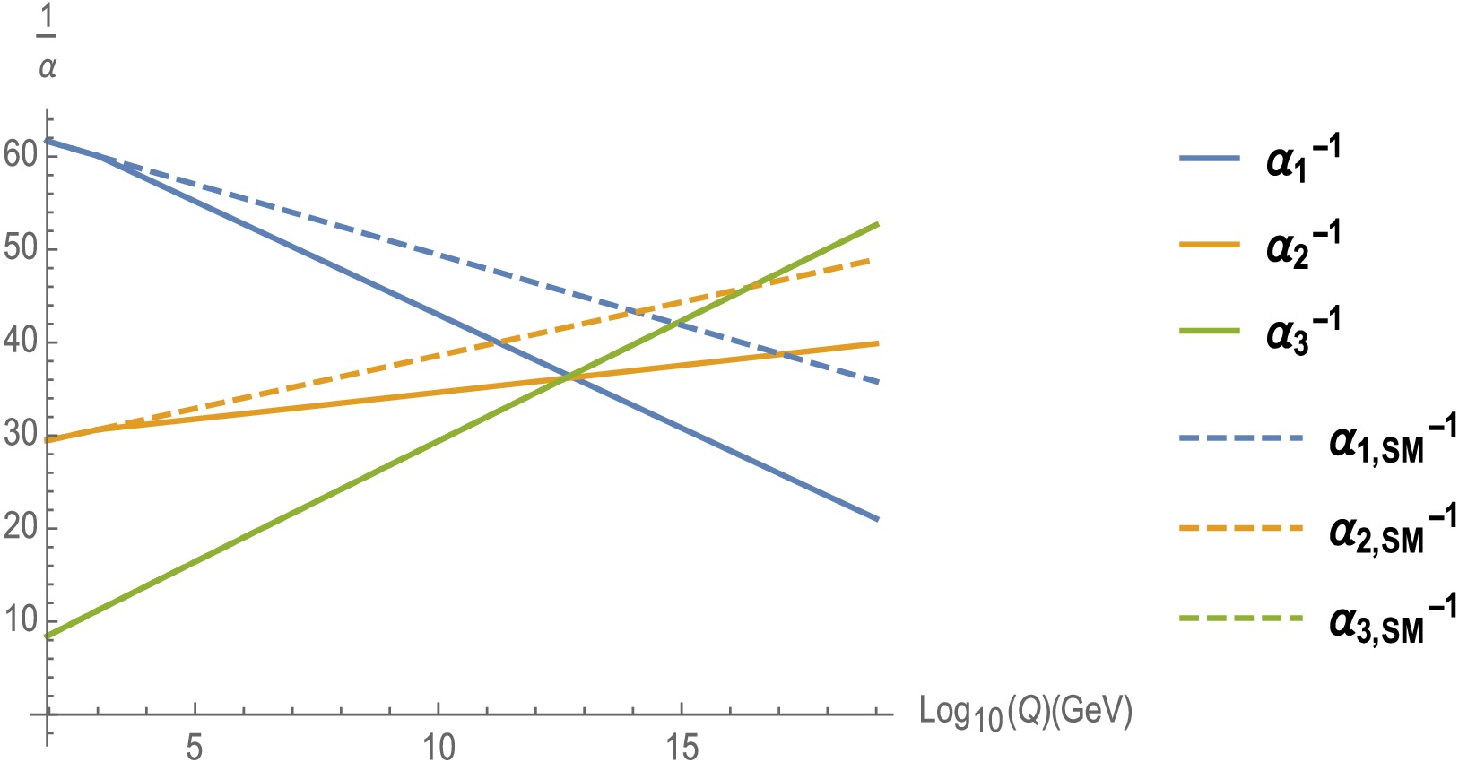
Figure 1. (color online) Running of couplings
$ g_1, g_2 $ , and$ g_3 $ and their unification at the 2-loop level, in terms of$ \alpha^{-1} $ , in the SM (dashed lines) versus BSM (solid lines). Blue, amber, and green represent$ g_1 $ ,$ g_2 $ , and$ g_3 $ , respectively. The BSM consists of an inert scalar doublet and two generations of$ Z_2 $ -odd vector-like leptons, with masses of$ {\cal{O}}(1 \; \text{TeV}) $ .The most stringent limit on proton lifetime comes from Super-Kamiokande [94], viz.,
$ \tau (p \to \pi^0 e^+) \gt 2.4 \times 10^{34} $ years. Although the proton lifetime is model-dependent, a naive estimate [95] is$ \tau \sim M_G^4/(\alpha_G^2 m_p^5) $ , where$ M_G $ is the unification scale,$ \alpha_G = \dfrac{g_G^2}{4\pi} $ ,$ g_G $ being the coupling value at$ M_G $ , and$ m_p $ is the proton mass. For$ 1/\alpha_G \sim 30 $ , we require$ M_G \gtrsim 6 \times 10^{15} $ GeV.With more scalars or vector-like leptons, the unification scale would be further decreased. The only plausible way to achieve
$ M_G \gtrsim 10^{16} $ GeV seems to be the addition of quarks. To estimate the scale of the exotic quarks for unification, we utilize the RGEs up to 1-loop, which are a set of three decoupled equations corresponding to the gauge couplings$ g_1 $ ,$ g_2 $ , and$ g_3 $ . The calculation is shown in Appendix B. Using these scales for defining the β-functions, we numerically solve the RGEs up to two loops, i.e., Eq. (24) for the couplings$ g_i $ . Out of the many solutions, two are plotted in Fig. 2.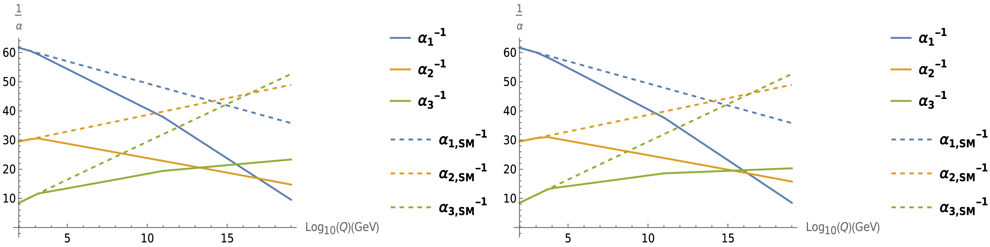
Figure 2. (color online) Running of couplings
$ g_1, g_2 $ , and$ g_3 $ , and their unification at the 2-loop level, in terms of$ \alpha^{-1} $ , in the SM (dashed lines) vs. the new model (solid lines). Blue, amber, and green represent$ g_1 $ ,$ g_2 $ , and$ g_3 $ , respectively. The two figures correspond to the following mass scales and number of generations for the$ Z_2 $ -odd quarks: Left:$ 2 \cdot 10^3 $ GeV ($ Q_{L/R} \times 2 $ and$ D^S_{L/R} \times 2 $ ) and$ 10^{11} $ GeV ($ U^S_{L/R} \times 2 $ ); Right:$ 5 \cdot 10^3 $ GeV ($ Q_{L/R} \times 2 $ ),$ 10^4 $ GeV ($ D^S_{L/R} \times 3 $ ), and$ 10^{11} $ GeV ($ U^S_{L/R} \times 2 $ ).In Fig. 2 (Left), we have considered two generations of each of the exotic quarks and found that a unification scale above
$ 10^{15} $ GeV requires the exotic singlet up-type quarks to be at a very high scale, just a few orders shy of the unification scale, while the exotic doublet quarks as well as the singlet down-type quarks must be close to the other$ Z_2 $ -odd particles5 . However, it is difficult to push the unification scale to$ 10^{16} $ GeV. Observing that the singlet down-type quark,$ D^S_{L/R} $ , considerably affects the slope of$ \alpha_3^{-1} $ while its effect on the slope of$ \alpha_1^{-1} $ is negligible, we are able to achieve unification at$ m_G \sim 10^{16} $ GeV6 by considering an extra generation of$ D^S_{L/R} $ . This is shown in Fig. 2 (Right). Similar results can be achieved by instead considering an extra generation of the doublet VL quarks ($ Q_{L/R} $ ) at somewhat different mass scales for the VL quarks. The interpretation of these results remains open, leaving room for curiosity. -
The presence of additional fermions and scalars affects the running of the gauge couplings above the TeV scale. The exotic particles contribute to the SM β-functions in the same way as the SM fermions and the Higgs doublet, with the exception that for the vector-like counterparts to the SM fermions, each contribution doubles since both left- and right-handed components contribute equally. The expressions are given in Appendix A.
To this order, the renormalization group equations (RGEs) for the couplings (
$ g_i $ ) can be expressed as$ \frac{{\rm d} g_i}{{\rm d} \ln Q}=\beta_i {(g_i)}, $
(24) where
$ \beta_i {(g_i)} $ are the β-functions and Q denotes the scale at which the couplings are being considered, with the boundary values fixed experimentally at$ Q = m_Z $ . For our purpose, it suffices to consider the β-functions up to two loops. At this level of accuracy, one could neglect threshold effects and include the contributions of a new species J only for$ Q \gt m_J $ . Within this approximation, thus, the β-functions would consist of a series of step functions.For
4 $ i=1,2,3 $ ,$ g_i $ denotes the coupling for$ U(1)_Y $ ,$ S U(2)_L $ , and$ S U(3)_C $ , respectively. To solve Eq. (24), we also take into account the contribution of the Top-Yukawa coupling,$ Y_t $ , and the scalar quartic coupling,$ \lambda_H $ , represented as$ g_4 $ and$ g_5 $ , respectively. Together with the equations for$ g_1, g_2, $ and$ g_3 $ , this gives us five coupled differential equations. Representing the scale by$ t=\ln Q $ such that$ t_0=\ln m_Z $ denotes the scale for SM,$ t_1 $ denotes the next higher energy scale at which one or more BSM particles are introduced, and so on, the equations can be solved numerically in each region$ (t_{n-1},t_n) $ to obtain the solutions$ g_i^{(n)} (t) $ , using the boundary conditions$ g_i^{(n)} (t_{n-1}) = g_i^{(n-1)} (t_{n-1}) $ .We assume the scale for
$ Z_2 $ -odd leptons and the scalar Φ as$ 1 $ TeV, while$ Z_2 $ -odd quarks are assumed to be much heavier such that there is a unification of the gauge couplings at a next higher scale ($ t_G $ ), given by the condition$ g_1 (t_G) = g_2 (t_G) = g_3 (t_G). $
(25) In Fig. 1, we first illustrate the unification of gauge couplings, considering only the inert scalar doublet and two generations of
$ Z_2 $ -odd vector-like leptons as the BSM content, all with masses of order$ {\cal O}(1\; \text{TeV}) $ . Without any BSM quarks, the slope of$ \alpha_3^{-1} $ is unchanged compared to the SM. On the other hand, the slopes of$ \alpha_1^{-1} $ and$ \alpha_2^{-1} $ increase as both receive positive contributions from the BSM. This lowers the scale of unification. We also observe that the presence of new particles raises the value of the unified gauge coupling. Embedding the model into grand unified theories may predict proton decay, which has not been observed experimentally.
Figure 1. (color online) Running of couplings
$ g_1, g_2 $ , and$ g_3 $ and their unification at the 2-loop level, in terms of$ \alpha^{-1} $ , in the SM (dashed lines) versus BSM (solid lines). Blue, amber, and green represent$ g_1 $ ,$ g_2 $ , and$ g_3 $ , respectively. The BSM consists of an inert scalar doublet and two generations of$ Z_2 $ -odd vector-like leptons, with masses of$ {\cal{O}}(1 \; \text{TeV}) $ .The most stringent limit on proton lifetime comes from Super-Kamiokande [94], viz.,
$ \tau (p \to \pi^0 e^+) \gt 2.4 \times 10^{34} $ years. Although the proton lifetime is model-dependent, a naive estimate [95] is$ \tau \sim M_G^4/(\alpha_G^2 m_p^5) $ , where$ M_G $ is the unification scale,$ \alpha_G = \dfrac{g_G^2}{4\pi} $ ,$ g_G $ being the coupling value at$ M_G $ , and$ m_p $ is the proton mass. For$ 1/\alpha_G \sim 30 $ , we require$ M_G \gtrsim 6 \times 10^{15} $ GeV.With more scalars or vector-like leptons, the unification scale would be further decreased. The only plausible way to achieve
$ M_G \gtrsim 10^{16} $ GeV seems to be the addition of quarks. To estimate the scale of the exotic quarks for unification, we utilize the RGEs up to 1-loop, which are a set of three decoupled equations corresponding to the gauge couplings$ g_1 $ ,$ g_2 $ , and$ g_3 $ . The calculation is shown in Appendix B. Using these scales for defining the β-functions, we numerically solve the RGEs up to two loops, i.e., Eq. (24) for the couplings$ g_i $ . Out of the many solutions, two are plotted in Fig. 2.
Figure 2. (color online) Running of couplings
$ g_1, g_2 $ , and$ g_3 $ , and their unification at the 2-loop level, in terms of$ \alpha^{-1} $ , in the SM (dashed lines) vs. the new model (solid lines). Blue, amber, and green represent$ g_1 $ ,$ g_2 $ , and$ g_3 $ , respectively. The two figures correspond to the following mass scales and number of generations for the$ Z_2 $ -odd quarks: Left:$ 2 \cdot 10^3 $ GeV ($ Q_{L/R} \times 2 $ and$ D^S_{L/R} \times 2 $ ) and$ 10^{11} $ GeV ($ U^S_{L/R} \times 2 $ ); Right:$ 5 \cdot 10^3 $ GeV ($ Q_{L/R} \times 2 $ ),$ 10^4 $ GeV ($ D^S_{L/R} \times 3 $ ), and$ 10^{11} $ GeV ($ U^S_{L/R} \times 2 $ ).In Fig. 2 (Left), we have considered two generations of each of the exotic quarks and found that a unification scale above
$ 10^{15} $ GeV requires the exotic singlet up-type quarks to be at a very high scale, just a few orders shy of the unification scale, while the exotic doublet quarks as well as the singlet down-type quarks must be close to the other$ Z_2 $ -odd particles5 . However, it is difficult to push the unification scale to$ 10^{16} $ GeV. Observing that the singlet down-type quark,$ D^S_{L/R} $ , considerably affects the slope of$ \alpha_3^{-1} $ while its effect on the slope of$ \alpha_1^{-1} $ is negligible, we are able to achieve unification at$ m_G \sim 10^{16} $ GeV6 by considering an extra generation of$ D^S_{L/R} $ . This is shown in Fig. 2 (Right). Similar results can be achieved by instead considering an extra generation of the doublet VL quarks ($ Q_{L/R} $ ) at somewhat different mass scales for the VL quarks. The interpretation of these results remains open, leaving room for curiosity. -
The presence of additional fermions and scalars affects the running of the gauge couplings above the TeV scale. The exotic particles contribute to the SM β-functions in the same way as the SM fermions and the Higgs doublet, with the exception that for the vector-like counterparts to the SM fermions, each contribution doubles since both left- and right-handed components contribute equally. The expressions are given in Appendix A.
To this order, the renormalization group equations (RGEs) for the couplings (
$ g_i $ ) can be expressed as$ \frac{{\rm d} g_i}{{\rm d} \ln Q}=\beta_i {(g_i)}, $
(24) where
$ \beta_i {(g_i)} $ are the β-functions and Q denotes the scale at which the couplings are being considered, with the boundary values fixed experimentally at$ Q = m_Z $ . For our purpose, it suffices to consider the β-functions up to two loops. At this level of accuracy, one could neglect threshold effects and include the contributions of a new species J only for$ Q \gt m_J $ . Within this approximation, thus, the β-functions would consist of a series of step functions.For
4 $ i=1,2,3 $ ,$ g_i $ denotes the coupling for$ U(1)_Y $ ,$ S U(2)_L $ , and$ S U(3)_C $ , respectively. To solve Eq. (24), we also take into account the contribution of the Top-Yukawa coupling,$ Y_t $ , and the scalar quartic coupling,$ \lambda_H $ , represented as$ g_4 $ and$ g_5 $ , respectively. Together with the equations for$ g_1, g_2, $ and$ g_3 $ , this gives us five coupled differential equations. Representing the scale by$ t=\ln Q $ such that$ t_0=\ln m_Z $ denotes the scale for SM,$ t_1 $ denotes the next higher energy scale at which one or more BSM particles are introduced, and so on, the equations can be solved numerically in each region$ (t_{n-1},t_n) $ to obtain the solutions$ g_i^{(n)} (t) $ , using the boundary conditions$ g_i^{(n)} (t_{n-1}) = g_i^{(n-1)} (t_{n-1}) $ .We assume the scale for
$ Z_2 $ -odd leptons and the scalar Φ as$ 1 $ TeV, while$ Z_2 $ -odd quarks are assumed to be much heavier such that there is a unification of the gauge couplings at a next higher scale ($ t_G $ ), given by the condition$ g_1 (t_G) = g_2 (t_G) = g_3 (t_G). $
(25) In Fig. 1, we first illustrate the unification of gauge couplings, considering only the inert scalar doublet and two generations of
$ Z_2 $ -odd vector-like leptons as the BSM content, all with masses of order$ {\cal O}(1\; \text{TeV}) $ . Without any BSM quarks, the slope of$ \alpha_3^{-1} $ is unchanged compared to the SM. On the other hand, the slopes of$ \alpha_1^{-1} $ and$ \alpha_2^{-1} $ increase as both receive positive contributions from the BSM. This lowers the scale of unification. We also observe that the presence of new particles raises the value of the unified gauge coupling. Embedding the model into grand unified theories may predict proton decay, which has not been observed experimentally.
Figure 1. (color online) Running of couplings
$ g_1, g_2 $ , and$ g_3 $ and their unification at the 2-loop level, in terms of$ \alpha^{-1} $ , in the SM (dashed lines) versus BSM (solid lines). Blue, amber, and green represent$ g_1 $ ,$ g_2 $ , and$ g_3 $ , respectively. The BSM consists of an inert scalar doublet and two generations of$ Z_2 $ -odd vector-like leptons, with masses of$ {\cal{O}}(1 \; \text{TeV}) $ .The most stringent limit on proton lifetime comes from Super-Kamiokande [94], viz.,
$ \tau (p \to \pi^0 e^+) \gt 2.4 \times 10^{34} $ years. Although the proton lifetime is model-dependent, a naive estimate [95] is$ \tau \sim M_G^4/(\alpha_G^2 m_p^5) $ , where$ M_G $ is the unification scale,$ \alpha_G = \dfrac{g_G^2}{4\pi} $ ,$ g_G $ being the coupling value at$ M_G $ , and$ m_p $ is the proton mass. For$ 1/\alpha_G \sim 30 $ , we require$ M_G \gtrsim 6 \times 10^{15} $ GeV.With more scalars or vector-like leptons, the unification scale would be further decreased. The only plausible way to achieve
$ M_G \gtrsim 10^{16} $ GeV seems to be the addition of quarks. To estimate the scale of the exotic quarks for unification, we utilize the RGEs up to 1-loop, which are a set of three decoupled equations corresponding to the gauge couplings$ g_1 $ ,$ g_2 $ , and$ g_3 $ . The calculation is shown in Appendix B. Using these scales for defining the β-functions, we numerically solve the RGEs up to two loops, i.e., Eq. (24) for the couplings$ g_i $ . Out of the many solutions, two are plotted in Fig. 2.
Figure 2. (color online) Running of couplings
$ g_1, g_2 $ , and$ g_3 $ , and their unification at the 2-loop level, in terms of$ \alpha^{-1} $ , in the SM (dashed lines) vs. the new model (solid lines). Blue, amber, and green represent$ g_1 $ ,$ g_2 $ , and$ g_3 $ , respectively. The two figures correspond to the following mass scales and number of generations for the$ Z_2 $ -odd quarks: Left:$ 2 \cdot 10^3 $ GeV ($ Q_{L/R} \times 2 $ and$ D^S_{L/R} \times 2 $ ) and$ 10^{11} $ GeV ($ U^S_{L/R} \times 2 $ ); Right:$ 5 \cdot 10^3 $ GeV ($ Q_{L/R} \times 2 $ ),$ 10^4 $ GeV ($ D^S_{L/R} \times 3 $ ), and$ 10^{11} $ GeV ($ U^S_{L/R} \times 2 $ ).In Fig. 2 (Left), we have considered two generations of each of the exotic quarks and found that a unification scale above
$ 10^{15} $ GeV requires the exotic singlet up-type quarks to be at a very high scale, just a few orders shy of the unification scale, while the exotic doublet quarks as well as the singlet down-type quarks must be close to the other$ Z_2 $ -odd particles5 . However, it is difficult to push the unification scale to$ 10^{16} $ GeV. Observing that the singlet down-type quark,$ D^S_{L/R} $ , considerably affects the slope of$ \alpha_3^{-1} $ while its effect on the slope of$ \alpha_1^{-1} $ is negligible, we are able to achieve unification at$ m_G \sim 10^{16} $ GeV6 by considering an extra generation of$ D^S_{L/R} $ . This is shown in Fig. 2 (Right). Similar results can be achieved by instead considering an extra generation of the doublet VL quarks ($ Q_{L/R} $ ) at somewhat different mass scales for the VL quarks. The interpretation of these results remains open, leaving room for curiosity. -
The presence of additional fermions and scalars affects the running of the gauge couplings above the TeV scale. The exotic particles contribute to the SM β-functions in the same way as the SM fermions and the Higgs doublet, with the exception that for the vector-like counterparts to the SM fermions, each contribution doubles since both left- and right-handed components contribute equally. The expressions are given in Appendix A.
To this order, the renormalization group equations (RGEs) for the couplings (
$ g_i $ ) can be expressed as$ \frac{{\rm d} g_i}{{\rm d} \ln Q}=\beta_i {(g_i)}, $
(24) where
$ \beta_i {(g_i)} $ are the β-functions and Q denotes the scale at which the couplings are being considered, with the boundary values fixed experimentally at$ Q = m_Z $ . For our purpose, it suffices to consider the β-functions up to two loops. At this level of accuracy, one could neglect threshold effects and include the contributions of a new species J only for$ Q \gt m_J $ . Within this approximation, thus, the β-functions would consist of a series of step functions.For
4 $ i=1,2,3 $ ,$ g_i $ denotes the coupling for$ U(1)_Y $ ,$ S U(2)_L $ , and$ S U(3)_C $ , respectively. To solve Eq. (24), we also take into account the contribution of the Top-Yukawa coupling,$ Y_t $ , and the scalar quartic coupling,$ \lambda_H $ , represented as$ g_4 $ and$ g_5 $ , respectively. Together with the equations for$ g_1, g_2, $ and$ g_3 $ , this gives us five coupled differential equations. Representing the scale by$ t=\ln Q $ such that$ t_0=\ln m_Z $ denotes the scale for SM,$ t_1 $ denotes the next higher energy scale at which one or more BSM particles are introduced, and so on, the equations can be solved numerically in each region$ (t_{n-1},t_n) $ to obtain the solutions$ g_i^{(n)} (t) $ , using the boundary conditions$ g_i^{(n)} (t_{n-1}) = g_i^{(n-1)} (t_{n-1}) $ .We assume the scale for
$ Z_2 $ -odd leptons and the scalar Φ as$ 1 $ TeV, while$ Z_2 $ -odd quarks are assumed to be much heavier such that there is a unification of the gauge couplings at a next higher scale ($ t_G $ ), given by the condition$ g_1 (t_G) = g_2 (t_G) = g_3 (t_G). $
(25) In Fig. 1, we first illustrate the unification of gauge couplings, considering only the inert scalar doublet and two generations of
$ Z_2 $ -odd vector-like leptons as the BSM content, all with masses of order$ {\cal O}(1\; \text{TeV}) $ . Without any BSM quarks, the slope of$ \alpha_3^{-1} $ is unchanged compared to the SM. On the other hand, the slopes of$ \alpha_1^{-1} $ and$ \alpha_2^{-1} $ increase as both receive positive contributions from the BSM. This lowers the scale of unification. We also observe that the presence of new particles raises the value of the unified gauge coupling. Embedding the model into grand unified theories may predict proton decay, which has not been observed experimentally.
Figure 1. (color online) Running of couplings
$ g_1, g_2 $ , and$ g_3 $ and their unification at the 2-loop level, in terms of$ \alpha^{-1} $ , in the SM (dashed lines) versus BSM (solid lines). Blue, amber, and green represent$ g_1 $ ,$ g_2 $ , and$ g_3 $ , respectively. The BSM consists of an inert scalar doublet and two generations of$ Z_2 $ -odd vector-like leptons, with masses of$ {\cal{O}}(1 \; \text{TeV}) $ .The most stringent limit on proton lifetime comes from Super-Kamiokande [94], viz.,
$ \tau (p \to \pi^0 e^+) \gt 2.4 \times 10^{34} $ years. Although the proton lifetime is model-dependent, a naive estimate [95] is$ \tau \sim M_G^4/(\alpha_G^2 m_p^5) $ , where$ M_G $ is the unification scale,$ \alpha_G = \dfrac{g_G^2}{4\pi} $ ,$ g_G $ being the coupling value at$ M_G $ , and$ m_p $ is the proton mass. For$ 1/\alpha_G \sim 30 $ , we require$ M_G \gtrsim 6 \times 10^{15} $ GeV.With more scalars or vector-like leptons, the unification scale would be further decreased. The only plausible way to achieve
$ M_G \gtrsim 10^{16} $ GeV seems to be the addition of quarks. To estimate the scale of the exotic quarks for unification, we utilize the RGEs up to 1-loop, which are a set of three decoupled equations corresponding to the gauge couplings$ g_1 $ ,$ g_2 $ , and$ g_3 $ . The calculation is shown in Appendix B. Using these scales for defining the β-functions, we numerically solve the RGEs up to two loops, i.e., Eq. (24) for the couplings$ g_i $ . Out of the many solutions, two are plotted in Fig. 2.
Figure 2. (color online) Running of couplings
$ g_1, g_2 $ , and$ g_3 $ , and their unification at the 2-loop level, in terms of$ \alpha^{-1} $ , in the SM (dashed lines) vs. the new model (solid lines). Blue, amber, and green represent$ g_1 $ ,$ g_2 $ , and$ g_3 $ , respectively. The two figures correspond to the following mass scales and number of generations for the$ Z_2 $ -odd quarks: Left:$ 2 \cdot 10^3 $ GeV ($ Q_{L/R} \times 2 $ and$ D^S_{L/R} \times 2 $ ) and$ 10^{11} $ GeV ($ U^S_{L/R} \times 2 $ ); Right:$ 5 \cdot 10^3 $ GeV ($ Q_{L/R} \times 2 $ ),$ 10^4 $ GeV ($ D^S_{L/R} \times 3 $ ), and$ 10^{11} $ GeV ($ U^S_{L/R} \times 2 $ ).In Fig. 2 (Left), we have considered two generations of each of the exotic quarks and found that a unification scale above
$ 10^{15} $ GeV requires the exotic singlet up-type quarks to be at a very high scale, just a few orders shy of the unification scale, while the exotic doublet quarks as well as the singlet down-type quarks must be close to the other$ Z_2 $ -odd particles5 . However, it is difficult to push the unification scale to$ 10^{16} $ GeV. Observing that the singlet down-type quark,$ D^S_{L/R} $ , considerably affects the slope of$ \alpha_3^{-1} $ while its effect on the slope of$ \alpha_1^{-1} $ is negligible, we are able to achieve unification at$ m_G \sim 10^{16} $ GeV6 by considering an extra generation of$ D^S_{L/R} $ . This is shown in Fig. 2 (Right). Similar results can be achieved by instead considering an extra generation of the doublet VL quarks ($ Q_{L/R} $ ) at somewhat different mass scales for the VL quarks. The interpretation of these results remains open, leaving room for curiosity. -
The presence of additional fermions and scalars affects the running of the gauge couplings above the TeV scale. The exotic particles contribute to the SM β-functions in the same way as the SM fermions and the Higgs doublet, with the exception that for the vector-like counterparts to the SM fermions, each contribution doubles since both left- and right-handed components contribute equally. The expressions are given in Appendix A.
To this order, the renormalization group equations (RGEs) for the couplings (
$ g_i $ ) can be expressed as$ \frac{{\rm d} g_i}{{\rm d} \ln Q}=\beta_i {(g_i)}, $
(24) where
$ \beta_i {(g_i)} $ are the β-functions and Q denotes the scale at which the couplings are being considered, with the boundary values fixed experimentally at$ Q = m_Z $ . For our purpose, it suffices to consider the β-functions up to two loops. At this level of accuracy, one could neglect threshold effects and include the contributions of a new species J only for$ Q \gt m_J $ . Within this approximation, thus, the β-functions would consist of a series of step functions.For
4 $ i=1,2,3 $ ,$ g_i $ denotes the coupling for$ U(1)_Y $ ,$ S U(2)_L $ , and$ S U(3)_C $ , respectively. To solve Eq. (24), we also take into account the contribution of the Top-Yukawa coupling,$ Y_t $ , and the scalar quartic coupling,$ \lambda_H $ , represented as$ g_4 $ and$ g_5 $ , respectively. Together with the equations for$ g_1, g_2, $ and$ g_3 $ , this gives us five coupled differential equations. Representing the scale by$ t=\ln Q $ such that$ t_0=\ln m_Z $ denotes the scale for SM,$ t_1 $ denotes the next higher energy scale at which one or more BSM particles are introduced, and so on, the equations can be solved numerically in each region$ (t_{n-1},t_n) $ to obtain the solutions$ g_i^{(n)} (t) $ , using the boundary conditions$ g_i^{(n)} (t_{n-1}) = g_i^{(n-1)} (t_{n-1}) $ .We assume the scale for
$ Z_2 $ -odd leptons and the scalar Φ as$ 1 $ TeV, while$ Z_2 $ -odd quarks are assumed to be much heavier such that there is a unification of the gauge couplings at a next higher scale ($ t_G $ ), given by the condition$ g_1 (t_G) = g_2 (t_G) = g_3 (t_G). $
(25) In Fig. 1, we first illustrate the unification of gauge couplings, considering only the inert scalar doublet and two generations of
$ Z_2 $ -odd vector-like leptons as the BSM content, all with masses of order$ {\cal O}(1\; \text{TeV}) $ . Without any BSM quarks, the slope of$ \alpha_3^{-1} $ is unchanged compared to the SM. On the other hand, the slopes of$ \alpha_1^{-1} $ and$ \alpha_2^{-1} $ increase as both receive positive contributions from the BSM. This lowers the scale of unification. We also observe that the presence of new particles raises the value of the unified gauge coupling. Embedding the model into grand unified theories may predict proton decay, which has not been observed experimentally.
Figure 1. (color online) Running of couplings
$ g_1, g_2 $ , and$ g_3 $ and their unification at the 2-loop level, in terms of$ \alpha^{-1} $ , in the SM (dashed lines) versus BSM (solid lines). Blue, amber, and green represent$ g_1 $ ,$ g_2 $ , and$ g_3 $ , respectively. The BSM consists of an inert scalar doublet and two generations of$ Z_2 $ -odd vector-like leptons, with masses of$ {\cal{O}}(1 \; \text{TeV}) $ .The most stringent limit on proton lifetime comes from Super-Kamiokande [94], viz.,
$ \tau (p \to \pi^0 e^+) \gt 2.4 \times 10^{34} $ years. Although the proton lifetime is model-dependent, a naive estimate [95] is$ \tau \sim M_G^4/(\alpha_G^2 m_p^5) $ , where$ M_G $ is the unification scale,$ \alpha_G = \dfrac{g_G^2}{4\pi} $ ,$ g_G $ being the coupling value at$ M_G $ , and$ m_p $ is the proton mass. For$ 1/\alpha_G \sim 30 $ , we require$ M_G \gtrsim 6 \times 10^{15} $ GeV.With more scalars or vector-like leptons, the unification scale would be further decreased. The only plausible way to achieve
$ M_G \gtrsim 10^{16} $ GeV seems to be the addition of quarks. To estimate the scale of the exotic quarks for unification, we utilize the RGEs up to 1-loop, which are a set of three decoupled equations corresponding to the gauge couplings$ g_1 $ ,$ g_2 $ , and$ g_3 $ . The calculation is shown in Appendix B. Using these scales for defining the β-functions, we numerically solve the RGEs up to two loops, i.e., Eq. (24) for the couplings$ g_i $ . Out of the many solutions, two are plotted in Fig. 2.
Figure 2. (color online) Running of couplings
$ g_1, g_2 $ , and$ g_3 $ , and their unification at the 2-loop level, in terms of$ \alpha^{-1} $ , in the SM (dashed lines) vs. the new model (solid lines). Blue, amber, and green represent$ g_1 $ ,$ g_2 $ , and$ g_3 $ , respectively. The two figures correspond to the following mass scales and number of generations for the$ Z_2 $ -odd quarks: Left:$ 2 \cdot 10^3 $ GeV ($ Q_{L/R} \times 2 $ and$ D^S_{L/R} \times 2 $ ) and$ 10^{11} $ GeV ($ U^S_{L/R} \times 2 $ ); Right:$ 5 \cdot 10^3 $ GeV ($ Q_{L/R} \times 2 $ ),$ 10^4 $ GeV ($ D^S_{L/R} \times 3 $ ), and$ 10^{11} $ GeV ($ U^S_{L/R} \times 2 $ ).In Fig. 2 (Left), we have considered two generations of each of the exotic quarks and found that a unification scale above
$ 10^{15} $ GeV requires the exotic singlet up-type quarks to be at a very high scale, just a few orders shy of the unification scale, while the exotic doublet quarks as well as the singlet down-type quarks must be close to the other$ Z_2 $ -odd particles5 . However, it is difficult to push the unification scale to$ 10^{16} $ GeV. Observing that the singlet down-type quark,$ D^S_{L/R} $ , considerably affects the slope of$ \alpha_3^{-1} $ while its effect on the slope of$ \alpha_1^{-1} $ is negligible, we are able to achieve unification at$ m_G \sim 10^{16} $ GeV6 by considering an extra generation of$ D^S_{L/R} $ . This is shown in Fig. 2 (Right). Similar results can be achieved by instead considering an extra generation of the doublet VL quarks ($ Q_{L/R} $ ) at somewhat different mass scales for the VL quarks. The interpretation of these results remains open, leaving room for curiosity. -
The presence of additional fermions and scalars affects the running of the gauge couplings above the TeV scale. The exotic particles contribute to the SM β-functions in the same way as the SM fermions and the Higgs doublet, with the exception that for the vector-like counterparts to the SM fermions, each contribution doubles since both left- and right-handed components contribute equally. The expressions are given in Appendix A.
To this order, the renormalization group equations (RGEs) for the couplings (
$ g_i $ ) can be expressed as$ \frac{{\rm d} g_i}{{\rm d} \ln Q}=\beta_i {(g_i)}, $
(24) where
$ \beta_i {(g_i)} $ are the β-functions and Q denotes the scale at which the couplings are being considered, with the boundary values fixed experimentally at$ Q = m_Z $ . For our purpose, it suffices to consider the β-functions up to two loops. At this level of accuracy, one could neglect threshold effects and include the contributions of a new species J only for$ Q \gt m_J $ . Within this approximation, thus, the β-functions would consist of a series of step functions.For
4 $ i=1,2,3 $ ,$ g_i $ denotes the coupling for$ U(1)_Y $ ,$ S U(2)_L $ , and$ S U(3)_C $ , respectively. To solve Eq. (24), we also take into account the contribution of the Top-Yukawa coupling,$ Y_t $ , and the scalar quartic coupling,$ \lambda_H $ , represented as$ g_4 $ and$ g_5 $ , respectively. Together with the equations for$ g_1, g_2, $ and$ g_3 $ , this gives us five coupled differential equations. Representing the scale by$ t=\ln Q $ such that$ t_0=\ln m_Z $ denotes the scale for SM,$ t_1 $ denotes the next higher energy scale at which one or more BSM particles are introduced, and so on, the equations can be solved numerically in each region$ (t_{n-1},t_n) $ to obtain the solutions$ g_i^{(n)} (t) $ , using the boundary conditions$ g_i^{(n)} (t_{n-1}) = g_i^{(n-1)} (t_{n-1}) $ .We assume the scale for
$ Z_2 $ -odd leptons and the scalar Φ as$ 1 $ TeV, while$ Z_2 $ -odd quarks are assumed to be much heavier such that there is a unification of the gauge couplings at a next higher scale ($ t_G $ ), given by the condition$ g_1 (t_G) = g_2 (t_G) = g_3 (t_G). $
(25) In Fig. 1, we first illustrate the unification of gauge couplings, considering only the inert scalar doublet and two generations of
$ Z_2 $ -odd vector-like leptons as the BSM content, all with masses of order$ {\cal O}(1\; \text{TeV}) $ . Without any BSM quarks, the slope of$ \alpha_3^{-1} $ is unchanged compared to the SM. On the other hand, the slopes of$ \alpha_1^{-1} $ and$ \alpha_2^{-1} $ increase as both receive positive contributions from the BSM. This lowers the scale of unification. We also observe that the presence of new particles raises the value of the unified gauge coupling. Embedding the model into grand unified theories may predict proton decay, which has not been observed experimentally.
Figure 1. (color online) Running of couplings
$ g_1, g_2 $ , and$ g_3 $ and their unification at the 2-loop level, in terms of$ \alpha^{-1} $ , in the SM (dashed lines) versus BSM (solid lines). Blue, amber, and green represent$ g_1 $ ,$ g_2 $ , and$ g_3 $ , respectively. The BSM consists of an inert scalar doublet and two generations of$ Z_2 $ -odd vector-like leptons, with masses of$ {\cal{O}}(1 \; \text{TeV}) $ .The most stringent limit on proton lifetime comes from Super-Kamiokande [94], viz.,
$ \tau (p \to \pi^0 e^+) \gt 2.4 \times 10^{34} $ years. Although the proton lifetime is model-dependent, a naive estimate [95] is$ \tau \sim M_G^4/(\alpha_G^2 m_p^5) $ , where$ M_G $ is the unification scale,$ \alpha_G = \dfrac{g_G^2}{4\pi} $ ,$ g_G $ being the coupling value at$ M_G $ , and$ m_p $ is the proton mass. For$ 1/\alpha_G \sim 30 $ , we require$ M_G \gtrsim 6 \times 10^{15} $ GeV.With more scalars or vector-like leptons, the unification scale would be further decreased. The only plausible way to achieve
$ M_G \gtrsim 10^{16} $ GeV seems to be the addition of quarks. To estimate the scale of the exotic quarks for unification, we utilize the RGEs up to 1-loop, which are a set of three decoupled equations corresponding to the gauge couplings$ g_1 $ ,$ g_2 $ , and$ g_3 $ . The calculation is shown in Appendix B. Using these scales for defining the β-functions, we numerically solve the RGEs up to two loops, i.e., Eq. (24) for the couplings$ g_i $ . Out of the many solutions, two are plotted in Fig. 2.
Figure 2. (color online) Running of couplings
$ g_1, g_2 $ , and$ g_3 $ , and their unification at the 2-loop level, in terms of$ \alpha^{-1} $ , in the SM (dashed lines) vs. the new model (solid lines). Blue, amber, and green represent$ g_1 $ ,$ g_2 $ , and$ g_3 $ , respectively. The two figures correspond to the following mass scales and number of generations for the$ Z_2 $ -odd quarks: Left:$ 2 \cdot 10^3 $ GeV ($ Q_{L/R} \times 2 $ and$ D^S_{L/R} \times 2 $ ) and$ 10^{11} $ GeV ($ U^S_{L/R} \times 2 $ ); Right:$ 5 \cdot 10^3 $ GeV ($ Q_{L/R} \times 2 $ ),$ 10^4 $ GeV ($ D^S_{L/R} \times 3 $ ), and$ 10^{11} $ GeV ($ U^S_{L/R} \times 2 $ ).In Fig. 2 (Left), we have considered two generations of each of the exotic quarks and found that a unification scale above
$ 10^{15} $ GeV requires the exotic singlet up-type quarks to be at a very high scale, just a few orders shy of the unification scale, while the exotic doublet quarks as well as the singlet down-type quarks must be close to the other$ Z_2 $ -odd particles5 . However, it is difficult to push the unification scale to$ 10^{16} $ GeV. Observing that the singlet down-type quark,$ D^S_{L/R} $ , considerably affects the slope of$ \alpha_3^{-1} $ while its effect on the slope of$ \alpha_1^{-1} $ is negligible, we are able to achieve unification at$ m_G \sim 10^{16} $ GeV6 by considering an extra generation of$ D^S_{L/R} $ . This is shown in Fig. 2 (Right). Similar results can be achieved by instead considering an extra generation of the doublet VL quarks ($ Q_{L/R} $ ) at somewhat different mass scales for the VL quarks. The interpretation of these results remains open, leaving room for curiosity. -
The presence of additional fermions and scalars affects the running of the gauge couplings above the TeV scale. The exotic particles contribute to the SM β-functions in the same way as the SM fermions and the Higgs doublet, with the exception that for the vector-like counterparts to the SM fermions, each contribution doubles since both left- and right-handed components contribute equally. The expressions are given in Appendix A.
To this order, the renormalization group equations (RGEs) for the couplings (
$ g_i $ ) can be expressed as$ \frac{{\rm d} g_i}{{\rm d} \ln Q}=\beta_i {(g_i)}, $
(24) where
$ \beta_i {(g_i)} $ are the β-functions and Q denotes the scale at which the couplings are being considered, with the boundary values fixed experimentally at$ Q = m_Z $ . For our purpose, it suffices to consider the β-functions up to two loops. At this level of accuracy, one could neglect threshold effects and include the contributions of a new species J only for$ Q \gt m_J $ . Within this approximation, thus, the β-functions would consist of a series of step functions.For
4 $ i=1,2,3 $ ,$ g_i $ denotes the coupling for$ U(1)_Y $ ,$ S U(2)_L $ , and$ S U(3)_C $ , respectively. To solve Eq. (24), we also take into account the contribution of the Top-Yukawa coupling,$ Y_t $ , and the scalar quartic coupling,$ \lambda_H $ , represented as$ g_4 $ and$ g_5 $ , respectively. Together with the equations for$ g_1, g_2, $ and$ g_3 $ , this gives us five coupled differential equations. Representing the scale by$ t=\ln Q $ such that$ t_0=\ln m_Z $ denotes the scale for SM,$ t_1 $ denotes the next higher energy scale at which one or more BSM particles are introduced, and so on, the equations can be solved numerically in each region$ (t_{n-1},t_n) $ to obtain the solutions$ g_i^{(n)} (t) $ , using the boundary conditions$ g_i^{(n)} (t_{n-1}) = g_i^{(n-1)} (t_{n-1}) $ .We assume the scale for
$ Z_2 $ -odd leptons and the scalar Φ as$ 1 $ TeV, while$ Z_2 $ -odd quarks are assumed to be much heavier such that there is a unification of the gauge couplings at a next higher scale ($ t_G $ ), given by the condition$ g_1 (t_G) = g_2 (t_G) = g_3 (t_G). $
(25) In Fig. 1, we first illustrate the unification of gauge couplings, considering only the inert scalar doublet and two generations of
$ Z_2 $ -odd vector-like leptons as the BSM content, all with masses of order$ {\cal O}(1\; \text{TeV}) $ . Without any BSM quarks, the slope of$ \alpha_3^{-1} $ is unchanged compared to the SM. On the other hand, the slopes of$ \alpha_1^{-1} $ and$ \alpha_2^{-1} $ increase as both receive positive contributions from the BSM. This lowers the scale of unification. We also observe that the presence of new particles raises the value of the unified gauge coupling. Embedding the model into grand unified theories may predict proton decay, which has not been observed experimentally.
Figure 1. (color online) Running of couplings
$ g_1, g_2 $ , and$ g_3 $ and their unification at the 2-loop level, in terms of$ \alpha^{-1} $ , in the SM (dashed lines) versus BSM (solid lines). Blue, amber, and green represent$ g_1 $ ,$ g_2 $ , and$ g_3 $ , respectively. The BSM consists of an inert scalar doublet and two generations of$ Z_2 $ -odd vector-like leptons, with masses of$ {\cal{O}}(1 \; \text{TeV}) $ .The most stringent limit on proton lifetime comes from Super-Kamiokande [94], viz.,
$ \tau (p \to \pi^0 e^+) \gt 2.4 \times 10^{34} $ years. Although the proton lifetime is model-dependent, a naive estimate [95] is$ \tau \sim M_G^4/(\alpha_G^2 m_p^5) $ , where$ M_G $ is the unification scale,$ \alpha_G = \dfrac{g_G^2}{4\pi} $ ,$ g_G $ being the coupling value at$ M_G $ , and$ m_p $ is the proton mass. For$ 1/\alpha_G \sim 30 $ , we require$ M_G \gtrsim 6 \times 10^{15} $ GeV.With more scalars or vector-like leptons, the unification scale would be further decreased. The only plausible way to achieve
$ M_G \gtrsim 10^{16} $ GeV seems to be the addition of quarks. To estimate the scale of the exotic quarks for unification, we utilize the RGEs up to 1-loop, which are a set of three decoupled equations corresponding to the gauge couplings$ g_1 $ ,$ g_2 $ , and$ g_3 $ . The calculation is shown in Appendix B. Using these scales for defining the β-functions, we numerically solve the RGEs up to two loops, i.e., Eq. (24) for the couplings$ g_i $ . Out of the many solutions, two are plotted in Fig. 2.
Figure 2. (color online) Running of couplings
$ g_1, g_2 $ , and$ g_3 $ , and their unification at the 2-loop level, in terms of$ \alpha^{-1} $ , in the SM (dashed lines) vs. the new model (solid lines). Blue, amber, and green represent$ g_1 $ ,$ g_2 $ , and$ g_3 $ , respectively. The two figures correspond to the following mass scales and number of generations for the$ Z_2 $ -odd quarks: Left:$ 2 \cdot 10^3 $ GeV ($ Q_{L/R} \times 2 $ and$ D^S_{L/R} \times 2 $ ) and$ 10^{11} $ GeV ($ U^S_{L/R} \times 2 $ ); Right:$ 5 \cdot 10^3 $ GeV ($ Q_{L/R} \times 2 $ ),$ 10^4 $ GeV ($ D^S_{L/R} \times 3 $ ), and$ 10^{11} $ GeV ($ U^S_{L/R} \times 2 $ ).In Fig. 2 (Left), we have considered two generations of each of the exotic quarks and found that a unification scale above
$ 10^{15} $ GeV requires the exotic singlet up-type quarks to be at a very high scale, just a few orders shy of the unification scale, while the exotic doublet quarks as well as the singlet down-type quarks must be close to the other$ Z_2 $ -odd particles5 . However, it is difficult to push the unification scale to$ 10^{16} $ GeV. Observing that the singlet down-type quark,$ D^S_{L/R} $ , considerably affects the slope of$ \alpha_3^{-1} $ while its effect on the slope of$ \alpha_1^{-1} $ is negligible, we are able to achieve unification at$ m_G \sim 10^{16} $ GeV6 by considering an extra generation of$ D^S_{L/R} $ . This is shown in Fig. 2 (Right). Similar results can be achieved by instead considering an extra generation of the doublet VL quarks ($ Q_{L/R} $ ) at somewhat different mass scales for the VL quarks. The interpretation of these results remains open, leaving room for curiosity. -
With the
$ Z_2 $ symmetry remaining unbroken, there are no mass terms connecting the SM neutrinos to the new fields; thus, the former remain exactly massless at the tree level. However, at the one-loop level, Weinberg operators are generated; the lepton number violation inherent to such operators is induced by the Majorana mass terms for the singlet fermions$ N_{\alpha R}^S $ . The generic Feynman diagram illustrating the generation of neutrino masses at the one-loop level is shown in Fig. 3, with all$ Z_2 $ -odd particles expressed in the mass basis. This kind of radiative generation of neutrino masses is reminiscent of the Scotogenic mechanism proposed in Refs. [30, 31]. The resultant contribution to the effective ($ 3\times 3 $ ) mass matrix for the light neutrino sector is given by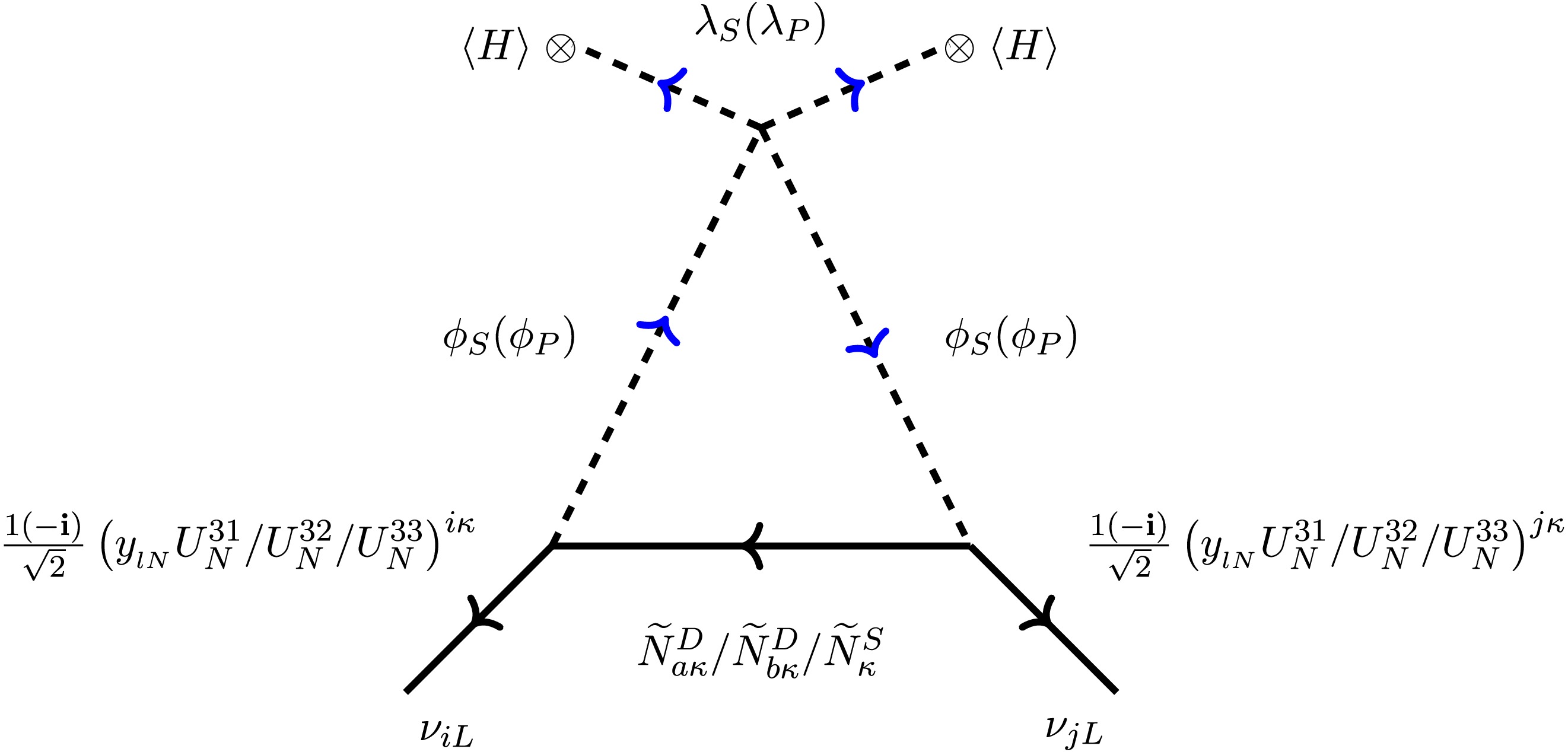
Figure 3. (color online) Feynman diagrams generate light neutrino masses at the 1-loop level. There are two diagrams arising from
$ \phi_S $ and$ \phi_P $ in the loop, respectively. Expressions corresponding to$ \phi_P $ are indicated in parentheses. The coupling combinations are given by$ \lambda_{S,P} \equiv -\frac{1}{4} \left(\lambda_1 + \lambda_2 \pm 2\lambda_3\right) $ . The indices$ \kappa=1,2 $ denote the generation index for the heavy neutrinos$ { \widetilde N^D}_X $ ,$ { \widetilde N^D}_Y $ , and$ \widetilde N^S $ each, while$ i,j=1-3 $ denote the SM generation indices.$ \frac{m_\nu}{\langle H \rangle^2}\; =\; \frac{\lambda_3}{16\pi^2} \,\, y_{{lN}} M_\Delta^{-1} y_{{lN}}^T, $
(26) where
$ M_\Delta^{-1} $ is a$ 2\times 2 $ symmetric complex matrix and to the leading order7 in$ \lambda_3 \, v^2/\mu_\Phi^2 $ , is given by$ \left( M_\Delta^{-1} \right)^{\alpha\beta}\; =\; \sum\limits_{\gamma} \left[ \frac{U_N^{\alpha^\prime \gamma}\, I \left( x_{\widetilde N_{\gamma}} \right)\,U_N^{\beta^\prime \gamma}}{m_{\widetilde N_{\gamma}}} \right]. $
(27) In the above equation, indices
$ \alpha,\beta=1,2 $ ,$ \alpha'=4+\alpha $ , and$ \beta'=4+\beta $ pertain to the gauge basis, whereas$ \gamma=1-6 $ represents the index for the mass basis.$ I \left(x_{\widetilde N_{\gamma}} \right) $ is the loop factor with$ x_{\widetilde N_{\gamma}}={m_{\phi_S}^2}/{m_{\widetilde N_{\gamma}}^2} $ and is given by$ I(x)\; =\; - \left({{\rm{ln}}}\,x+1-x \right) \left(x-1 \right)^{-2} $ . Please note that the analytical forms of the mixing matrices, as derived in Sec. II.B.3, are presented in the form of$ 2 \times 2 $ block matrices, utilizing the$ 2 \times 2 $ Yukawa couplings outlined in Eq. (8). Consequently, it would be advantageous to compute the Feynman diagrams for radiative neutrino mass generation in this section and for lepton flavor violation and charged lepton$ g-2 $ in the subsequent section, employing the$ 2 \times 2 $ blocks of the mixing matrix. This approach will facilitate the obtaining of analytical results, expressed in terms of the Yukawa couplings. Thus, expanding the mass basis as$ \widetilde N $ =$\{ { \widetilde N^D}_X $ ,$ { \widetilde N^D}_Y $ ,$ \widetilde N^S \}$ and writing out these contributions more explicitly,$ \begin{aligned}[b]\left( M_\Delta^{-1} \right)^{\alpha\beta}\; =\;&\Big[ U_N^{31}{\cal D}_{\widetilde N_{a}^D}\left(U_N^{31}\right)^T + U_N^{32}{\cal D}_{\widetilde N_{b}^D}\left(U_N^{31}\right)^T \\&+ U_N^{33}{\cal D}_{\widetilde N^S}\left(U_N^{33}\right)^T\Big]^{\alpha \beta},\end{aligned} $
(28) where we have denoted
$ 2 \times 2 $ blocks for mixing of$ N^S_R $ with each of$ { \widetilde N^D}_{a} $ ,$ { \widetilde N^D}_Y $ , and$ \widetilde N^S $ as$ U_N^{ij} $ —the '$ ij^{th} $ '$ 2 \times 2 $ block of the$ 6 \times 6 $ mixing matrix$ U_N $ ($ =U_N^0 U_N^1 $ ) for the exotic neutral fermion sector (see equations (12), (16), (17) and (19)). The factor$ {I \left(x_{\widetilde N_{\gamma}} \right)}/{m_{\widetilde N_{\gamma}}} $ is encapsulated into$ 2 \times 2 $ diagonal matrices$ {\cal D}_Y={{\rm{Diag}}}\left[\dfrac{I \left(x_{Y_1} \right)}{m_{Y_1}}, \dfrac{I \left(x_{Y_2} \right)}{m_{Y_2}}\right] $ . For TeV-scale masses of the$ Z_2 $ -odd (pseudo)scalars and Majorana neutrinos, i.e.,$ x\; \sim\; {\cal O} \left(1 \right) $ , the loop factor$ I(x) $ can be estimated to be of$ {\cal O} \left(1 \right) $ 8 . Hence,$ \left(M_\Delta^{-1} \right)^{\alpha\beta}\; \sim\; {\cal O} \left({{\rm{TeV}}}^{-1} \right) $ . Therefore, naively, one can estimate from Eq. (26) that$ y_{lN}\; \sim\; {\cal O} \left(10^{-5} \right) $ and$ \lambda_3\; \sim\; 0.1 $ result in neutrino masses of$ {\cal O} \left(0.1\; {{\rm{eV}}} \right) $ . It is important to note that$ y_{lN}\; \sim\; {\cal O} \left(10^{-1} \right) $ is also allowed, provided$ \lambda_3\; \sim\; {\cal O} \left(10^{-9} \right) $ .In view of the relatively complicated structure of the neutrino mass matrix,
$ m_\nu $ , in Eq. (26), it is instructive to look for an approximate simplified expression for$ m_\nu $ in the simplified scenario (i.e.,$ m_L\; =\; \widetilde m_L\times I_{2\times 2} $ and$ m_N = \widetilde m_N\times I_{2\times 2} $ ) discussed in the previous section. In the limit,$ \left(M_{\Delta}^{-1} \right)^{\alpha \beta}\; \sim\; { \widetilde m_N}^{-1} I \left(m_{\phi_S}^2/{ \widetilde m_N}^2 \right) \, \delta^{\alpha\beta} $ (up to the leading order in$ z_{{LN}} $ ), the neutrino mass matrix in Eq. (26) can be approximated as:$ \frac{m_\nu}{\langle H \rangle^2}\; \sim\; \frac{\lambda_3}{16\pi^2 \widetilde m_N} I \left( \frac{m_{\phi_S}^2}{{ \widetilde m_N}^2} \right) \, y_{{lN}} y_{{lN}}^T. $
(29) -
With the
$ Z_2 $ symmetry remaining unbroken, there are no mass terms connecting the SM neutrinos to the new fields; thus, the former remain exactly massless at the tree level. However, at the one-loop level, Weinberg operators are generated; the lepton number violation inherent to such operators is induced by the Majorana mass terms for the singlet fermions$ N_{\alpha R}^S $ . The generic Feynman diagram illustrating the generation of neutrino masses at the one-loop level is shown in Fig. 3, with all$ Z_2 $ -odd particles expressed in the mass basis. This kind of radiative generation of neutrino masses is reminiscent of the Scotogenic mechanism proposed in Refs. [30, 31]. The resultant contribution to the effective ($ 3\times 3 $ ) mass matrix for the light neutrino sector is given by
Figure 3. (color online) Feynman diagrams generate light neutrino masses at the 1-loop level. There are two diagrams arising from
$ \phi_S $ and$ \phi_P $ in the loop, respectively. Expressions corresponding to$ \phi_P $ are indicated in parentheses. The coupling combinations are given by$ \lambda_{S,P} \equiv -\frac{1}{4} \left(\lambda_1 + \lambda_2 \pm 2\lambda_3\right) $ . The indices$ \kappa=1,2 $ denote the generation index for the heavy neutrinos$ { \widetilde N^D}_X $ ,$ { \widetilde N^D}_Y $ , and$ \widetilde N^S $ each, while$ i,j=1-3 $ denote the SM generation indices.$ \frac{m_\nu}{\langle H \rangle^2}\; =\; \frac{\lambda_3}{16\pi^2} \,\, y_{{lN}} M_\Delta^{-1} y_{{lN}}^T, $
(26) where
$ M_\Delta^{-1} $ is a$ 2\times 2 $ symmetric complex matrix and to the leading order7 in$ \lambda_3 \, v^2/\mu_\Phi^2 $ , is given by$ \left( M_\Delta^{-1} \right)^{\alpha\beta}\; =\; \sum\limits_{\gamma} \left[ \frac{U_N^{\alpha^\prime \gamma}\, I \left( x_{\widetilde N_{\gamma}} \right)\,U_N^{\beta^\prime \gamma}}{m_{\widetilde N_{\gamma}}} \right]. $
(27) In the above equation, indices
$ \alpha,\beta=1,2 $ ,$ \alpha'=4+\alpha $ , and$ \beta'=4+\beta $ pertain to the gauge basis, whereas$ \gamma=1-6 $ represents the index for the mass basis.$ I \left(x_{\widetilde N_{\gamma}} \right) $ is the loop factor with$ x_{\widetilde N_{\gamma}}={m_{\phi_S}^2}/{m_{\widetilde N_{\gamma}}^2} $ and is given by$ I(x)\; =\; - \left({{\rm{ln}}}\,x+1-x \right) \left(x-1 \right)^{-2} $ . Please note that the analytical forms of the mixing matrices, as derived in Sec. II.B.3, are presented in the form of$ 2 \times 2 $ block matrices, utilizing the$ 2 \times 2 $ Yukawa couplings outlined in Eq. (8). Consequently, it would be advantageous to compute the Feynman diagrams for radiative neutrino mass generation in this section and for lepton flavor violation and charged lepton$ g-2 $ in the subsequent section, employing the$ 2 \times 2 $ blocks of the mixing matrix. This approach will facilitate the obtaining of analytical results, expressed in terms of the Yukawa couplings. Thus, expanding the mass basis as$ \widetilde N $ =$\{ { \widetilde N^D}_X $ ,$ { \widetilde N^D}_Y $ ,$ \widetilde N^S \}$ and writing out these contributions more explicitly,$ \begin{aligned}[b]\left( M_\Delta^{-1} \right)^{\alpha\beta}\; =\;&\Big[ U_N^{31}{\cal D}_{\widetilde N_{a}^D}\left(U_N^{31}\right)^T + U_N^{32}{\cal D}_{\widetilde N_{b}^D}\left(U_N^{31}\right)^T \\&+ U_N^{33}{\cal D}_{\widetilde N^S}\left(U_N^{33}\right)^T\Big]^{\alpha \beta},\end{aligned} $
(28) where we have denoted
$ 2 \times 2 $ blocks for mixing of$ N^S_R $ with each of$ { \widetilde N^D}_{a} $ ,$ { \widetilde N^D}_Y $ , and$ \widetilde N^S $ as$ U_N^{ij} $ —the '$ ij^{th} $ '$ 2 \times 2 $ block of the$ 6 \times 6 $ mixing matrix$ U_N $ ($ =U_N^0 U_N^1 $ ) for the exotic neutral fermion sector (see equations (12), (16), (17) and (19)). The factor$ {I \left(x_{\widetilde N_{\gamma}} \right)}/{m_{\widetilde N_{\gamma}}} $ is encapsulated into$ 2 \times 2 $ diagonal matrices$ {\cal D}_Y={{\rm{Diag}}}\left[\dfrac{I \left(x_{Y_1} \right)}{m_{Y_1}}, \dfrac{I \left(x_{Y_2} \right)}{m_{Y_2}}\right] $ . For TeV-scale masses of the$ Z_2 $ -odd (pseudo)scalars and Majorana neutrinos, i.e.,$ x\; \sim\; {\cal O} \left(1 \right) $ , the loop factor$ I(x) $ can be estimated to be of$ {\cal O} \left(1 \right) $ 8 . Hence,$ \left(M_\Delta^{-1} \right)^{\alpha\beta}\; \sim\; {\cal O} \left({{\rm{TeV}}}^{-1} \right) $ . Therefore, naively, one can estimate from Eq. (26) that$ y_{lN}\; \sim\; {\cal O} \left(10^{-5} \right) $ and$ \lambda_3\; \sim\; 0.1 $ result in neutrino masses of$ {\cal O} \left(0.1\; {{\rm{eV}}} \right) $ . It is important to note that$ y_{lN}\; \sim\; {\cal O} \left(10^{-1} \right) $ is also allowed, provided$ \lambda_3\; \sim\; {\cal O} \left(10^{-9} \right) $ .In view of the relatively complicated structure of the neutrino mass matrix,
$ m_\nu $ , in Eq. (26), it is instructive to look for an approximate simplified expression for$ m_\nu $ in the simplified scenario (i.e.,$ m_L\; =\; \widetilde m_L\times I_{2\times 2} $ and$ m_N = \widetilde m_N\times I_{2\times 2} $ ) discussed in the previous section. In the limit,$ \left(M_{\Delta}^{-1} \right)^{\alpha \beta}\; \sim\; { \widetilde m_N}^{-1} I \left(m_{\phi_S}^2/{ \widetilde m_N}^2 \right) \, \delta^{\alpha\beta} $ (up to the leading order in$ z_{{LN}} $ ), the neutrino mass matrix in Eq. (26) can be approximated as:$ \frac{m_\nu}{\langle H \rangle^2}\; \sim\; \frac{\lambda_3}{16\pi^2 \widetilde m_N} I \left( \frac{m_{\phi_S}^2}{{ \widetilde m_N}^2} \right) \, y_{{lN}} y_{{lN}}^T. $
(29) -
With the
$ Z_2 $ symmetry remaining unbroken, there are no mass terms connecting the SM neutrinos to the new fields; thus, the former remain exactly massless at the tree level. However, at the one-loop level, Weinberg operators are generated; the lepton number violation inherent to such operators is induced by the Majorana mass terms for the singlet fermions$ N_{\alpha R}^S $ . The generic Feynman diagram illustrating the generation of neutrino masses at the one-loop level is shown in Fig. 3, with all$ Z_2 $ -odd particles expressed in the mass basis. This kind of radiative generation of neutrino masses is reminiscent of the Scotogenic mechanism proposed in Refs. [30, 31]. The resultant contribution to the effective ($ 3\times 3 $ ) mass matrix for the light neutrino sector is given by
Figure 3. (color online) Feynman diagrams generate light neutrino masses at the 1-loop level. There are two diagrams arising from
$ \phi_S $ and$ \phi_P $ in the loop, respectively. Expressions corresponding to$ \phi_P $ are indicated in parentheses. The coupling combinations are given by$ \lambda_{S,P} \equiv -\frac{1}{4} \left(\lambda_1 + \lambda_2 \pm 2\lambda_3\right) $ . The indices$ \kappa=1,2 $ denote the generation index for the heavy neutrinos$ { \widetilde N^D}_X $ ,$ { \widetilde N^D}_Y $ , and$ \widetilde N^S $ each, while$ i,j=1-3 $ denote the SM generation indices.$ \frac{m_\nu}{\langle H \rangle^2}\; =\; \frac{\lambda_3}{16\pi^2} \,\, y_{{lN}} M_\Delta^{-1} y_{{lN}}^T, $
(26) where
$ M_\Delta^{-1} $ is a$ 2\times 2 $ symmetric complex matrix and to the leading order7 in$ \lambda_3 \, v^2/\mu_\Phi^2 $ , is given by$ \left( M_\Delta^{-1} \right)^{\alpha\beta}\; =\; \sum\limits_{\gamma} \left[ \frac{U_N^{\alpha^\prime \gamma}\, I \left( x_{\widetilde N_{\gamma}} \right)\,U_N^{\beta^\prime \gamma}}{m_{\widetilde N_{\gamma}}} \right]. $
(27) In the above equation, indices
$ \alpha,\beta=1,2 $ ,$ \alpha'=4+\alpha $ , and$ \beta'=4+\beta $ pertain to the gauge basis, whereas$ \gamma=1-6 $ represents the index for the mass basis.$ I \left(x_{\widetilde N_{\gamma}} \right) $ is the loop factor with$ x_{\widetilde N_{\gamma}}={m_{\phi_S}^2}/{m_{\widetilde N_{\gamma}}^2} $ and is given by$ I(x)\; =\; - \left({{\rm{ln}}}\,x+1-x \right) \left(x-1 \right)^{-2} $ . Please note that the analytical forms of the mixing matrices, as derived in Sec. II.B.3, are presented in the form of$ 2 \times 2 $ block matrices, utilizing the$ 2 \times 2 $ Yukawa couplings outlined in Eq. (8). Consequently, it would be advantageous to compute the Feynman diagrams for radiative neutrino mass generation in this section and for lepton flavor violation and charged lepton$ g-2 $ in the subsequent section, employing the$ 2 \times 2 $ blocks of the mixing matrix. This approach will facilitate the obtaining of analytical results, expressed in terms of the Yukawa couplings. Thus, expanding the mass basis as$ \widetilde N $ =$\{ { \widetilde N^D}_X $ ,$ { \widetilde N^D}_Y $ ,$ \widetilde N^S \}$ and writing out these contributions more explicitly,$ \begin{aligned}[b]\left( M_\Delta^{-1} \right)^{\alpha\beta}\; =\;&\Big[ U_N^{31}{\cal D}_{\widetilde N_{a}^D}\left(U_N^{31}\right)^T + U_N^{32}{\cal D}_{\widetilde N_{b}^D}\left(U_N^{31}\right)^T \\&+ U_N^{33}{\cal D}_{\widetilde N^S}\left(U_N^{33}\right)^T\Big]^{\alpha \beta},\end{aligned} $
(28) where we have denoted
$ 2 \times 2 $ blocks for mixing of$ N^S_R $ with each of$ { \widetilde N^D}_{a} $ ,$ { \widetilde N^D}_Y $ , and$ \widetilde N^S $ as$ U_N^{ij} $ —the '$ ij^{th} $ '$ 2 \times 2 $ block of the$ 6 \times 6 $ mixing matrix$ U_N $ ($ =U_N^0 U_N^1 $ ) for the exotic neutral fermion sector (see equations (12), (16), (17) and (19)). The factor$ {I \left(x_{\widetilde N_{\gamma}} \right)}/{m_{\widetilde N_{\gamma}}} $ is encapsulated into$ 2 \times 2 $ diagonal matrices$ {\cal D}_Y={{\rm{Diag}}}\left[\dfrac{I \left(x_{Y_1} \right)}{m_{Y_1}}, \dfrac{I \left(x_{Y_2} \right)}{m_{Y_2}}\right] $ . For TeV-scale masses of the$ Z_2 $ -odd (pseudo)scalars and Majorana neutrinos, i.e.,$ x\; \sim\; {\cal O} \left(1 \right) $ , the loop factor$ I(x) $ can be estimated to be of$ {\cal O} \left(1 \right) $ 8 . Hence,$ \left(M_\Delta^{-1} \right)^{\alpha\beta}\; \sim\; {\cal O} \left({{\rm{TeV}}}^{-1} \right) $ . Therefore, naively, one can estimate from Eq. (26) that$ y_{lN}\; \sim\; {\cal O} \left(10^{-5} \right) $ and$ \lambda_3\; \sim\; 0.1 $ result in neutrino masses of$ {\cal O} \left(0.1\; {{\rm{eV}}} \right) $ . It is important to note that$ y_{lN}\; \sim\; {\cal O} \left(10^{-1} \right) $ is also allowed, provided$ \lambda_3\; \sim\; {\cal O} \left(10^{-9} \right) $ .In view of the relatively complicated structure of the neutrino mass matrix,
$ m_\nu $ , in Eq. (26), it is instructive to look for an approximate simplified expression for$ m_\nu $ in the simplified scenario (i.e.,$ m_L\; =\; \widetilde m_L\times I_{2\times 2} $ and$ m_N = \widetilde m_N\times I_{2\times 2} $ ) discussed in the previous section. In the limit,$ \left(M_{\Delta}^{-1} \right)^{\alpha \beta}\; \sim\; { \widetilde m_N}^{-1} I \left(m_{\phi_S}^2/{ \widetilde m_N}^2 \right) \, \delta^{\alpha\beta} $ (up to the leading order in$ z_{{LN}} $ ), the neutrino mass matrix in Eq. (26) can be approximated as:$ \frac{m_\nu}{\langle H \rangle^2}\; \sim\; \frac{\lambda_3}{16\pi^2 \widetilde m_N} I \left( \frac{m_{\phi_S}^2}{{ \widetilde m_N}^2} \right) \, y_{{lN}} y_{{lN}}^T. $
(29) -
With the
$ Z_2 $ symmetry remaining unbroken, there are no mass terms connecting the SM neutrinos to the new fields; thus, the former remain exactly massless at the tree level. However, at the one-loop level, Weinberg operators are generated; the lepton number violation inherent to such operators is induced by the Majorana mass terms for the singlet fermions$ N_{\alpha R}^S $ . The generic Feynman diagram illustrating the generation of neutrino masses at the one-loop level is shown in Fig. 3, with all$ Z_2 $ -odd particles expressed in the mass basis. This kind of radiative generation of neutrino masses is reminiscent of the Scotogenic mechanism proposed in Refs. [30, 31]. The resultant contribution to the effective ($ 3\times 3 $ ) mass matrix for the light neutrino sector is given by
Figure 3. (color online) Feynman diagrams generate light neutrino masses at the 1-loop level. There are two diagrams arising from
$ \phi_S $ and$ \phi_P $ in the loop, respectively. Expressions corresponding to$ \phi_P $ are indicated in parentheses. The coupling combinations are given by$ \lambda_{S,P} \equiv -\frac{1}{4} \left(\lambda_1 + \lambda_2 \pm 2\lambda_3\right) $ . The indices$ \kappa=1,2 $ denote the generation index for the heavy neutrinos$ { \widetilde N^D}_X $ ,$ { \widetilde N^D}_Y $ , and$ \widetilde N^S $ each, while$ i,j=1-3 $ denote the SM generation indices.$ \frac{m_\nu}{\langle H \rangle^2}\; =\; \frac{\lambda_3}{16\pi^2} \,\, y_{{lN}} M_\Delta^{-1} y_{{lN}}^T, $
(26) where
$ M_\Delta^{-1} $ is a$ 2\times 2 $ symmetric complex matrix and to the leading order7 in$ \lambda_3 \, v^2/\mu_\Phi^2 $ , is given by$ \left( M_\Delta^{-1} \right)^{\alpha\beta}\; =\; \sum\limits_{\gamma} \left[ \frac{U_N^{\alpha^\prime \gamma}\, I \left( x_{\widetilde N_{\gamma}} \right)\,U_N^{\beta^\prime \gamma}}{m_{\widetilde N_{\gamma}}} \right]. $
(27) In the above equation, indices
$ \alpha,\beta=1,2 $ ,$ \alpha'=4+\alpha $ , and$ \beta'=4+\beta $ pertain to the gauge basis, whereas$ \gamma=1-6 $ represents the index for the mass basis.$ I \left(x_{\widetilde N_{\gamma}} \right) $ is the loop factor with$ x_{\widetilde N_{\gamma}}={m_{\phi_S}^2}/{m_{\widetilde N_{\gamma}}^2} $ and is given by$ I(x)\; =\; - \left({{\rm{ln}}}\,x+1-x \right) \left(x-1 \right)^{-2} $ . Please note that the analytical forms of the mixing matrices, as derived in Sec. II.B.3, are presented in the form of$ 2 \times 2 $ block matrices, utilizing the$ 2 \times 2 $ Yukawa couplings outlined in Eq. (8). Consequently, it would be advantageous to compute the Feynman diagrams for radiative neutrino mass generation in this section and for lepton flavor violation and charged lepton$ g-2 $ in the subsequent section, employing the$ 2 \times 2 $ blocks of the mixing matrix. This approach will facilitate the obtaining of analytical results, expressed in terms of the Yukawa couplings. Thus, expanding the mass basis as$ \widetilde N $ =$\{ { \widetilde N^D}_X $ ,$ { \widetilde N^D}_Y $ ,$ \widetilde N^S \}$ and writing out these contributions more explicitly,$ \begin{aligned}[b]\left( M_\Delta^{-1} \right)^{\alpha\beta}\; =\;&\Big[ U_N^{31}{\cal D}_{\widetilde N_{a}^D}\left(U_N^{31}\right)^T + U_N^{32}{\cal D}_{\widetilde N_{b}^D}\left(U_N^{31}\right)^T \\&+ U_N^{33}{\cal D}_{\widetilde N^S}\left(U_N^{33}\right)^T\Big]^{\alpha \beta},\end{aligned} $
(28) where we have denoted
$ 2 \times 2 $ blocks for mixing of$ N^S_R $ with each of$ { \widetilde N^D}_{a} $ ,$ { \widetilde N^D}_Y $ , and$ \widetilde N^S $ as$ U_N^{ij} $ —the '$ ij^{th} $ '$ 2 \times 2 $ block of the$ 6 \times 6 $ mixing matrix$ U_N $ ($ =U_N^0 U_N^1 $ ) for the exotic neutral fermion sector (see equations (12), (16), (17) and (19)). The factor$ {I \left(x_{\widetilde N_{\gamma}} \right)}/{m_{\widetilde N_{\gamma}}} $ is encapsulated into$ 2 \times 2 $ diagonal matrices$ {\cal D}_Y={{\rm{Diag}}}\left[\dfrac{I \left(x_{Y_1} \right)}{m_{Y_1}}, \dfrac{I \left(x_{Y_2} \right)}{m_{Y_2}}\right] $ . For TeV-scale masses of the$ Z_2 $ -odd (pseudo)scalars and Majorana neutrinos, i.e.,$ x\; \sim\; {\cal O} \left(1 \right) $ , the loop factor$ I(x) $ can be estimated to be of$ {\cal O} \left(1 \right) $ 8 . Hence,$ \left(M_\Delta^{-1} \right)^{\alpha\beta}\; \sim\; {\cal O} \left({{\rm{TeV}}}^{-1} \right) $ . Therefore, naively, one can estimate from Eq. (26) that$ y_{lN}\; \sim\; {\cal O} \left(10^{-5} \right) $ and$ \lambda_3\; \sim\; 0.1 $ result in neutrino masses of$ {\cal O} \left(0.1\; {{\rm{eV}}} \right) $ . It is important to note that$ y_{lN}\; \sim\; {\cal O} \left(10^{-1} \right) $ is also allowed, provided$ \lambda_3\; \sim\; {\cal O} \left(10^{-9} \right) $ .In view of the relatively complicated structure of the neutrino mass matrix,
$ m_\nu $ , in Eq. (26), it is instructive to look for an approximate simplified expression for$ m_\nu $ in the simplified scenario (i.e.,$ m_L\; =\; \widetilde m_L\times I_{2\times 2} $ and$ m_N = \widetilde m_N\times I_{2\times 2} $ ) discussed in the previous section. In the limit,$ \left(M_{\Delta}^{-1} \right)^{\alpha \beta}\; \sim\; { \widetilde m_N}^{-1} I \left(m_{\phi_S}^2/{ \widetilde m_N}^2 \right) \, \delta^{\alpha\beta} $ (up to the leading order in$ z_{{LN}} $ ), the neutrino mass matrix in Eq. (26) can be approximated as:$ \frac{m_\nu}{\langle H \rangle^2}\; \sim\; \frac{\lambda_3}{16\pi^2 \widetilde m_N} I \left( \frac{m_{\phi_S}^2}{{ \widetilde m_N}^2} \right) \, y_{{lN}} y_{{lN}}^T. $
(29) -
With the
$ Z_2 $ symmetry remaining unbroken, there are no mass terms connecting the SM neutrinos to the new fields; thus, the former remain exactly massless at the tree level. However, at the one-loop level, Weinberg operators are generated; the lepton number violation inherent to such operators is induced by the Majorana mass terms for the singlet fermions$ N_{\alpha R}^S $ . The generic Feynman diagram illustrating the generation of neutrino masses at the one-loop level is shown in Fig. 3, with all$ Z_2 $ -odd particles expressed in the mass basis. This kind of radiative generation of neutrino masses is reminiscent of the Scotogenic mechanism proposed in Refs. [30, 31]. The resultant contribution to the effective ($ 3\times 3 $ ) mass matrix for the light neutrino sector is given by
Figure 3. (color online) Feynman diagrams generate light neutrino masses at the 1-loop level. There are two diagrams arising from
$ \phi_S $ and$ \phi_P $ in the loop, respectively. Expressions corresponding to$ \phi_P $ are indicated in parentheses. The coupling combinations are given by$ \lambda_{S,P} \equiv -\frac{1}{4} \left(\lambda_1 + \lambda_2 \pm 2\lambda_3\right) $ . The indices$ \kappa=1,2 $ denote the generation index for the heavy neutrinos$ { \widetilde N^D}_X $ ,$ { \widetilde N^D}_Y $ , and$ \widetilde N^S $ each, while$ i,j=1-3 $ denote the SM generation indices.$ \frac{m_\nu}{\langle H \rangle^2}\; =\; \frac{\lambda_3}{16\pi^2} \,\, y_{{lN}} M_\Delta^{-1} y_{{lN}}^T, $
(26) where
$ M_\Delta^{-1} $ is a$ 2\times 2 $ symmetric complex matrix and to the leading order7 in$ \lambda_3 \, v^2/\mu_\Phi^2 $ , is given by$ \left( M_\Delta^{-1} \right)^{\alpha\beta}\; =\; \sum\limits_{\gamma} \left[ \frac{U_N^{\alpha^\prime \gamma}\, I \left( x_{\widetilde N_{\gamma}} \right)\,U_N^{\beta^\prime \gamma}}{m_{\widetilde N_{\gamma}}} \right]. $
(27) In the above equation, indices
$ \alpha,\beta=1,2 $ ,$ \alpha'=4+\alpha $ , and$ \beta'=4+\beta $ pertain to the gauge basis, whereas$ \gamma=1-6 $ represents the index for the mass basis.$ I \left(x_{\widetilde N_{\gamma}} \right) $ is the loop factor with$ x_{\widetilde N_{\gamma}}={m_{\phi_S}^2}/{m_{\widetilde N_{\gamma}}^2} $ and is given by$ I(x)\; =\; - \left({{\rm{ln}}}\,x+1-x \right) \left(x-1 \right)^{-2} $ . Please note that the analytical forms of the mixing matrices, as derived in Sec. II.B.3, are presented in the form of$ 2 \times 2 $ block matrices, utilizing the$ 2 \times 2 $ Yukawa couplings outlined in Eq. (8). Consequently, it would be advantageous to compute the Feynman diagrams for radiative neutrino mass generation in this section and for lepton flavor violation and charged lepton$ g-2 $ in the subsequent section, employing the$ 2 \times 2 $ blocks of the mixing matrix. This approach will facilitate the obtaining of analytical results, expressed in terms of the Yukawa couplings. Thus, expanding the mass basis as$ \widetilde N $ =$\{ { \widetilde N^D}_X $ ,$ { \widetilde N^D}_Y $ ,$ \widetilde N^S \}$ and writing out these contributions more explicitly,$ \begin{aligned}[b]\left( M_\Delta^{-1} \right)^{\alpha\beta}\; =\;&\Big[ U_N^{31}{\cal D}_{\widetilde N_{a}^D}\left(U_N^{31}\right)^T + U_N^{32}{\cal D}_{\widetilde N_{b}^D}\left(U_N^{31}\right)^T \\&+ U_N^{33}{\cal D}_{\widetilde N^S}\left(U_N^{33}\right)^T\Big]^{\alpha \beta},\end{aligned} $
(28) where we have denoted
$ 2 \times 2 $ blocks for mixing of$ N^S_R $ with each of$ { \widetilde N^D}_{a} $ ,$ { \widetilde N^D}_Y $ , and$ \widetilde N^S $ as$ U_N^{ij} $ —the '$ ij^{th} $ '$ 2 \times 2 $ block of the$ 6 \times 6 $ mixing matrix$ U_N $ ($ =U_N^0 U_N^1 $ ) for the exotic neutral fermion sector (see equations (12), (16), (17) and (19)). The factor$ {I \left(x_{\widetilde N_{\gamma}} \right)}/{m_{\widetilde N_{\gamma}}} $ is encapsulated into$ 2 \times 2 $ diagonal matrices$ {\cal D}_Y={{\rm{Diag}}}\left[\dfrac{I \left(x_{Y_1} \right)}{m_{Y_1}}, \dfrac{I \left(x_{Y_2} \right)}{m_{Y_2}}\right] $ . For TeV-scale masses of the$ Z_2 $ -odd (pseudo)scalars and Majorana neutrinos, i.e.,$ x\; \sim\; {\cal O} \left(1 \right) $ , the loop factor$ I(x) $ can be estimated to be of$ {\cal O} \left(1 \right) $ 8 . Hence,$ \left(M_\Delta^{-1} \right)^{\alpha\beta}\; \sim\; {\cal O} \left({{\rm{TeV}}}^{-1} \right) $ . Therefore, naively, one can estimate from Eq. (26) that$ y_{lN}\; \sim\; {\cal O} \left(10^{-5} \right) $ and$ \lambda_3\; \sim\; 0.1 $ result in neutrino masses of$ {\cal O} \left(0.1\; {{\rm{eV}}} \right) $ . It is important to note that$ y_{lN}\; \sim\; {\cal O} \left(10^{-1} \right) $ is also allowed, provided$ \lambda_3\; \sim\; {\cal O} \left(10^{-9} \right) $ .In view of the relatively complicated structure of the neutrino mass matrix,
$ m_\nu $ , in Eq. (26), it is instructive to look for an approximate simplified expression for$ m_\nu $ in the simplified scenario (i.e.,$ m_L\; =\; \widetilde m_L\times I_{2\times 2} $ and$ m_N = \widetilde m_N\times I_{2\times 2} $ ) discussed in the previous section. In the limit,$ \left(M_{\Delta}^{-1} \right)^{\alpha \beta}\; \sim\; { \widetilde m_N}^{-1} I \left(m_{\phi_S}^2/{ \widetilde m_N}^2 \right) \, \delta^{\alpha\beta} $ (up to the leading order in$ z_{{LN}} $ ), the neutrino mass matrix in Eq. (26) can be approximated as:$ \frac{m_\nu}{\langle H \rangle^2}\; \sim\; \frac{\lambda_3}{16\pi^2 \widetilde m_N} I \left( \frac{m_{\phi_S}^2}{{ \widetilde m_N}^2} \right) \, y_{{lN}} y_{{lN}}^T. $
(29) -
With the
$ Z_2 $ symmetry remaining unbroken, there are no mass terms connecting the SM neutrinos to the new fields; thus, the former remain exactly massless at the tree level. However, at the one-loop level, Weinberg operators are generated; the lepton number violation inherent to such operators is induced by the Majorana mass terms for the singlet fermions$ N_{\alpha R}^S $ . The generic Feynman diagram illustrating the generation of neutrino masses at the one-loop level is shown in Fig. 3, with all$ Z_2 $ -odd particles expressed in the mass basis. This kind of radiative generation of neutrino masses is reminiscent of the Scotogenic mechanism proposed in Refs. [30, 31]. The resultant contribution to the effective ($ 3\times 3 $ ) mass matrix for the light neutrino sector is given by
Figure 3. (color online) Feynman diagrams generate light neutrino masses at the 1-loop level. There are two diagrams arising from
$ \phi_S $ and$ \phi_P $ in the loop, respectively. Expressions corresponding to$ \phi_P $ are indicated in parentheses. The coupling combinations are given by$ \lambda_{S,P} \equiv -\frac{1}{4} \left(\lambda_1 + \lambda_2 \pm 2\lambda_3\right) $ . The indices$ \kappa=1,2 $ denote the generation index for the heavy neutrinos$ { \widetilde N^D}_X $ ,$ { \widetilde N^D}_Y $ , and$ \widetilde N^S $ each, while$ i,j=1-3 $ denote the SM generation indices.$ \frac{m_\nu}{\langle H \rangle^2}\; =\; \frac{\lambda_3}{16\pi^2} \,\, y_{{lN}} M_\Delta^{-1} y_{{lN}}^T, $
(26) where
$ M_\Delta^{-1} $ is a$ 2\times 2 $ symmetric complex matrix and to the leading order7 in$ \lambda_3 \, v^2/\mu_\Phi^2 $ , is given by$ \left( M_\Delta^{-1} \right)^{\alpha\beta}\; =\; \sum\limits_{\gamma} \left[ \frac{U_N^{\alpha^\prime \gamma}\, I \left( x_{\widetilde N_{\gamma}} \right)\,U_N^{\beta^\prime \gamma}}{m_{\widetilde N_{\gamma}}} \right]. $
(27) In the above equation, indices
$ \alpha,\beta=1,2 $ ,$ \alpha'=4+\alpha $ , and$ \beta'=4+\beta $ pertain to the gauge basis, whereas$ \gamma=1-6 $ represents the index for the mass basis.$ I \left(x_{\widetilde N_{\gamma}} \right) $ is the loop factor with$ x_{\widetilde N_{\gamma}}={m_{\phi_S}^2}/{m_{\widetilde N_{\gamma}}^2} $ and is given by$ I(x)\; =\; - \left({{\rm{ln}}}\,x+1-x \right) \left(x-1 \right)^{-2} $ . Please note that the analytical forms of the mixing matrices, as derived in Sec. II.B.3, are presented in the form of$ 2 \times 2 $ block matrices, utilizing the$ 2 \times 2 $ Yukawa couplings outlined in Eq. (8). Consequently, it would be advantageous to compute the Feynman diagrams for radiative neutrino mass generation in this section and for lepton flavor violation and charged lepton$ g-2 $ in the subsequent section, employing the$ 2 \times 2 $ blocks of the mixing matrix. This approach will facilitate the obtaining of analytical results, expressed in terms of the Yukawa couplings. Thus, expanding the mass basis as$ \widetilde N $ =$\{ { \widetilde N^D}_X $ ,$ { \widetilde N^D}_Y $ ,$ \widetilde N^S \}$ and writing out these contributions more explicitly,$ \begin{aligned}[b]\left( M_\Delta^{-1} \right)^{\alpha\beta}\; =\;&\Big[ U_N^{31}{\cal D}_{\widetilde N_{a}^D}\left(U_N^{31}\right)^T + U_N^{32}{\cal D}_{\widetilde N_{b}^D}\left(U_N^{31}\right)^T \\&+ U_N^{33}{\cal D}_{\widetilde N^S}\left(U_N^{33}\right)^T\Big]^{\alpha \beta},\end{aligned} $
(28) where we have denoted
$ 2 \times 2 $ blocks for mixing of$ N^S_R $ with each of$ { \widetilde N^D}_{a} $ ,$ { \widetilde N^D}_Y $ , and$ \widetilde N^S $ as$ U_N^{ij} $ —the '$ ij^{th} $ '$ 2 \times 2 $ block of the$ 6 \times 6 $ mixing matrix$ U_N $ ($ =U_N^0 U_N^1 $ ) for the exotic neutral fermion sector (see equations (12), (16), (17) and (19)). The factor$ {I \left(x_{\widetilde N_{\gamma}} \right)}/{m_{\widetilde N_{\gamma}}} $ is encapsulated into$ 2 \times 2 $ diagonal matrices$ {\cal D}_Y={{\rm{Diag}}}\left[\dfrac{I \left(x_{Y_1} \right)}{m_{Y_1}}, \dfrac{I \left(x_{Y_2} \right)}{m_{Y_2}}\right] $ . For TeV-scale masses of the$ Z_2 $ -odd (pseudo)scalars and Majorana neutrinos, i.e.,$ x\; \sim\; {\cal O} \left(1 \right) $ , the loop factor$ I(x) $ can be estimated to be of$ {\cal O} \left(1 \right) $ 8 . Hence,$ \left(M_\Delta^{-1} \right)^{\alpha\beta}\; \sim\; {\cal O} \left({{\rm{TeV}}}^{-1} \right) $ . Therefore, naively, one can estimate from Eq. (26) that$ y_{lN}\; \sim\; {\cal O} \left(10^{-5} \right) $ and$ \lambda_3\; \sim\; 0.1 $ result in neutrino masses of$ {\cal O} \left(0.1\; {{\rm{eV}}} \right) $ . It is important to note that$ y_{lN}\; \sim\; {\cal O} \left(10^{-1} \right) $ is also allowed, provided$ \lambda_3\; \sim\; {\cal O} \left(10^{-9} \right) $ .In view of the relatively complicated structure of the neutrino mass matrix,
$ m_\nu $ , in Eq. (26), it is instructive to look for an approximate simplified expression for$ m_\nu $ in the simplified scenario (i.e.,$ m_L\; =\; \widetilde m_L\times I_{2\times 2} $ and$ m_N = \widetilde m_N\times I_{2\times 2} $ ) discussed in the previous section. In the limit,$ \left(M_{\Delta}^{-1} \right)^{\alpha \beta}\; \sim\; { \widetilde m_N}^{-1} I \left(m_{\phi_S}^2/{ \widetilde m_N}^2 \right) \, \delta^{\alpha\beta} $ (up to the leading order in$ z_{{LN}} $ ), the neutrino mass matrix in Eq. (26) can be approximated as:$ \frac{m_\nu}{\langle H \rangle^2}\; \sim\; \frac{\lambda_3}{16\pi^2 \widetilde m_N} I \left( \frac{m_{\phi_S}^2}{{ \widetilde m_N}^2} \right) \, y_{{lN}} y_{{lN}}^T. $
(29) -
With the
$ Z_2 $ symmetry remaining unbroken, there are no mass terms connecting the SM neutrinos to the new fields; thus, the former remain exactly massless at the tree level. However, at the one-loop level, Weinberg operators are generated; the lepton number violation inherent to such operators is induced by the Majorana mass terms for the singlet fermions$ N_{\alpha R}^S $ . The generic Feynman diagram illustrating the generation of neutrino masses at the one-loop level is shown in Fig. 3, with all$ Z_2 $ -odd particles expressed in the mass basis. This kind of radiative generation of neutrino masses is reminiscent of the Scotogenic mechanism proposed in Refs. [30, 31]. The resultant contribution to the effective ($ 3\times 3 $ ) mass matrix for the light neutrino sector is given by
Figure 3. (color online) Feynman diagrams generate light neutrino masses at the 1-loop level. There are two diagrams arising from
$ \phi_S $ and$ \phi_P $ in the loop, respectively. Expressions corresponding to$ \phi_P $ are indicated in parentheses. The coupling combinations are given by$ \lambda_{S,P} \equiv -\frac{1}{4} \left(\lambda_1 + \lambda_2 \pm 2\lambda_3\right) $ . The indices$ \kappa=1,2 $ denote the generation index for the heavy neutrinos$ { \widetilde N^D}_X $ ,$ { \widetilde N^D}_Y $ , and$ \widetilde N^S $ each, while$ i,j=1-3 $ denote the SM generation indices.$ \frac{m_\nu}{\langle H \rangle^2}\; =\; \frac{\lambda_3}{16\pi^2} \,\, y_{{lN}} M_\Delta^{-1} y_{{lN}}^T, $
(26) where
$ M_\Delta^{-1} $ is a$ 2\times 2 $ symmetric complex matrix and to the leading order7 in$ \lambda_3 \, v^2/\mu_\Phi^2 $ , is given by$ \left( M_\Delta^{-1} \right)^{\alpha\beta}\; =\; \sum\limits_{\gamma} \left[ \frac{U_N^{\alpha^\prime \gamma}\, I \left( x_{\widetilde N_{\gamma}} \right)\,U_N^{\beta^\prime \gamma}}{m_{\widetilde N_{\gamma}}} \right]. $
(27) In the above equation, indices
$ \alpha,\beta=1,2 $ ,$ \alpha'=4+\alpha $ , and$ \beta'=4+\beta $ pertain to the gauge basis, whereas$ \gamma=1-6 $ represents the index for the mass basis.$ I \left(x_{\widetilde N_{\gamma}} \right) $ is the loop factor with$ x_{\widetilde N_{\gamma}}={m_{\phi_S}^2}/{m_{\widetilde N_{\gamma}}^2} $ and is given by$ I(x)\; =\; - \left({{\rm{ln}}}\,x+1-x \right) \left(x-1 \right)^{-2} $ . Please note that the analytical forms of the mixing matrices, as derived in Sec. II.B.3, are presented in the form of$ 2 \times 2 $ block matrices, utilizing the$ 2 \times 2 $ Yukawa couplings outlined in Eq. (8). Consequently, it would be advantageous to compute the Feynman diagrams for radiative neutrino mass generation in this section and for lepton flavor violation and charged lepton$ g-2 $ in the subsequent section, employing the$ 2 \times 2 $ blocks of the mixing matrix. This approach will facilitate the obtaining of analytical results, expressed in terms of the Yukawa couplings. Thus, expanding the mass basis as$ \widetilde N $ =$\{ { \widetilde N^D}_X $ ,$ { \widetilde N^D}_Y $ ,$ \widetilde N^S \}$ and writing out these contributions more explicitly,$ \begin{aligned}[b]\left( M_\Delta^{-1} \right)^{\alpha\beta}\; =\;&\Big[ U_N^{31}{\cal D}_{\widetilde N_{a}^D}\left(U_N^{31}\right)^T + U_N^{32}{\cal D}_{\widetilde N_{b}^D}\left(U_N^{31}\right)^T \\&+ U_N^{33}{\cal D}_{\widetilde N^S}\left(U_N^{33}\right)^T\Big]^{\alpha \beta},\end{aligned} $
(28) where we have denoted
$ 2 \times 2 $ blocks for mixing of$ N^S_R $ with each of$ { \widetilde N^D}_{a} $ ,$ { \widetilde N^D}_Y $ , and$ \widetilde N^S $ as$ U_N^{ij} $ —the '$ ij^{th} $ '$ 2 \times 2 $ block of the$ 6 \times 6 $ mixing matrix$ U_N $ ($ =U_N^0 U_N^1 $ ) for the exotic neutral fermion sector (see equations (12), (16), (17) and (19)). The factor$ {I \left(x_{\widetilde N_{\gamma}} \right)}/{m_{\widetilde N_{\gamma}}} $ is encapsulated into$ 2 \times 2 $ diagonal matrices$ {\cal D}_Y={{\rm{Diag}}}\left[\dfrac{I \left(x_{Y_1} \right)}{m_{Y_1}}, \dfrac{I \left(x_{Y_2} \right)}{m_{Y_2}}\right] $ . For TeV-scale masses of the$ Z_2 $ -odd (pseudo)scalars and Majorana neutrinos, i.e.,$ x\; \sim\; {\cal O} \left(1 \right) $ , the loop factor$ I(x) $ can be estimated to be of$ {\cal O} \left(1 \right) $ 8 . Hence,$ \left(M_\Delta^{-1} \right)^{\alpha\beta}\; \sim\; {\cal O} \left({{\rm{TeV}}}^{-1} \right) $ . Therefore, naively, one can estimate from Eq. (26) that$ y_{lN}\; \sim\; {\cal O} \left(10^{-5} \right) $ and$ \lambda_3\; \sim\; 0.1 $ result in neutrino masses of$ {\cal O} \left(0.1\; {{\rm{eV}}} \right) $ . It is important to note that$ y_{lN}\; \sim\; {\cal O} \left(10^{-1} \right) $ is also allowed, provided$ \lambda_3\; \sim\; {\cal O} \left(10^{-9} \right) $ .In view of the relatively complicated structure of the neutrino mass matrix,
$ m_\nu $ , in Eq. (26), it is instructive to look for an approximate simplified expression for$ m_\nu $ in the simplified scenario (i.e.,$ m_L\; =\; \widetilde m_L\times I_{2\times 2} $ and$ m_N = \widetilde m_N\times I_{2\times 2} $ ) discussed in the previous section. In the limit,$ \left(M_{\Delta}^{-1} \right)^{\alpha \beta}\; \sim\; { \widetilde m_N}^{-1} I \left(m_{\phi_S}^2/{ \widetilde m_N}^2 \right) \, \delta^{\alpha\beta} $ (up to the leading order in$ z_{{LN}} $ ), the neutrino mass matrix in Eq. (26) can be approximated as:$ \frac{m_\nu}{\langle H \rangle^2}\; \sim\; \frac{\lambda_3}{16\pi^2 \widetilde m_N} I \left( \frac{m_{\phi_S}^2}{{ \widetilde m_N}^2} \right) \, y_{{lN}} y_{{lN}}^T. $
(29) -
In the low energy effective theory, the neutrino mass matrix is determined by 9 parameters (3 neutrino masses, 3 mixing angles, and 3 phases). Decomposing into mixings and masses,
$ m_\nu $ on the left-hand side of Eq. (26) can be written as$ U^*_{MNS}D_\nu U_{MNS}^\dagger $ , where$ D_\nu = {{\rm{diag}}}\left(m_1, m_2, m_3\right) $ with$ m_1, m_2 $ , and$ m_3 $ being the masses of the SM neutrinos, and$ U_{MNS} $ is the Pontecorvo–Maki–Nakagawa–Sakata matrix [96, 97]. Therefore, Eq. (26) can be expressed as$ \frac{v^2\lambda_3}{16\pi^2} \,\, y_{{lN}} M_\Delta^{-1} y_{{lN}}^T = U^*_{MNS}D_\nu U_{MNS}^\dagger. $
(30) The matrix
$ U_{MNS} $ consists of three angles and three phases (one Dirac phase and two Majorana phases), in general. However, with two generations of$ N^S_R $ , the matrix$ y_{{lN}} $ is$ 3 \times 2 $ and$ M_\Delta^{-1} $ , which encodes the heavy neutrino mass parameter$ m_N $ , is$ 2 \times 2 $ . Thus, the matrix structure on the LHS is$ (3 \times 2)(2 \times 2)(2 \times 3) $ , which renders one light neutrino massless and one Majorana phase in$ U_{MNS} $ unphysical on the RHS. Therefore, the low-energy theory can provide information on seven parameters, in principle. On the other hand, the$ 3 \times 2 $ complex matrix$ y_{{lN}} $ contains 12 real parameters, of which three phases can be eliminated by a redefinition of the SM lepton doublet$ l_L $ , in a basis where the SM charged lepton mass matrix and$ m_N $ are diagonal. Thus,$ y_{{lN}} $ contains nine independent real parameters. The mass parameter$ m_N $ 9 is determined by two additional parameters. However, these are not independent of the nine parameters describing$ y_{{lN}} $ in view of the scaling symmetry10 of Eq. (26). Therefore, there are nine parameters at the high scale that determine the leading-order light neutrino mass matrix,$ m_\nu $ , at the low scale via the radiative seesaw mechanism. Since the number of parameters in the high-energy theory is larger than the number of parameters describing the low-energy neutrino phenomenology, proper parameterization [98–100] of the Yukawa matrix,$ y_{{lN}} $ , is required to ensure the consistency of the model with the available results from neutrino oscillation experiments. In this regard, Eq. (30) can be rewritten as:$\begin{aligned}[b]& \left[ \frac{v \sqrt{\lambda_3}}{4\pi} \, D_{\sqrt\nu}^{-1}\, U^T_{MNS}\, y_{{lN}}\, M_{\sqrt\Delta}^{-1} \right] \,\\& \times \left[ \frac{v \sqrt{\lambda_3}}{4\pi}\, \left( M_{\sqrt\Delta}^{-1} \right)^T\, y_{{lN}}^T \,U_{MNS} \,D_{\sqrt\nu}^{-1}\right]\; =\; {{\bf{I}}}_{3\times 3},\end{aligned} $
(31) where
$ D_{\sqrt \nu}^{-1} = {{\rm{diag}}}\left(m_1^{-\frac{1}{2}}, m_2^{-\frac{1}{2}}, m_3^{-\frac{1}{2}}\right) $ .$ M_{\Delta}^{-1} $ , being a complex symmetric matrix, can be diagonalized by a unitary matrix$ U_{\Delta} $ as$ M_{\Delta,d}^{-1} = U_\Delta^T M_\Delta^{-1} U_\Delta $ , where$ M_{\Delta,d}^{-1} $ is a diagonal$ 2\times 2 $ matrix. Therefore,$ M_{\Delta}^{-1} = U_\Delta^* M_{\Delta,d}^{-1} U_\Delta^{\dagger} = M_{\sqrt \Delta}^{-1} \left(M_{\sqrt\Delta}^{-1} \right)^{T} $ , where$ M_{\sqrt \Delta}^{-1} = U_\Delta^{*} M_{\sqrt{\Delta,d}}^{-1} $ . The most general Yukawa matrix$ y_{{lN}} $ which is consistent with the physical, low-energy neutrino parameters, viz., the three light neutrino masses ($ m_1 $ ,$ m_2 $ , and$ m_3 $ ), and the mixing angles as well as phases (contained in$ U_{MNS} $ ) is,${ \begin{array}{*{20}{c}} {}&{{y_{lN}}}\\ {}& \uparrow \\ {\# \ {\rm{of}}\;{\rm{Parameters}}:}&{12 - 3} \end{array}\begin{array}{*{20}{c}} = \\ {}\\ = \end{array}\begin{array}{*{20}{c}} { = \left( {\frac{{4\pi }}{v}\lambda _3^{ - \frac{1}{2}}} \right)}&{U_{MNS}^*}&{{D_{\sqrt \nu }}}&R&{{M_{\sqrt \Delta }},}\\ {}& \uparrow & \uparrow & \uparrow &{}\\ {}&5&2&2&{} \end{array}}$
where R is a complex
$ 3 \times 2 $ matrix subjected to the condition$ R\,R^T = {1}_{3 \times 3} $ . It is important to note that with one massless neutrino, the RHS of Eq. (31) has only two non-zero diagonal elements. Thus,$ RR^T = {{\rm{diag}}} \left(0,1,1 \right) $ for NH and$ {{\rm{diag}}} \left(1,1,0 \right) $ for IH. Consequently, R is described by 2 independent real parameters that bridge the gap between the low- and high-energy theories describing the light neutrino masses. In the simplified scenario,$\begin{aligned}[b]& M_{\sqrt \Delta} = { \left[ \frac{ \widetilde m_N} {I \left( \dfrac{m_{\phi_S}^2}{ \widetilde m_N^2} \right)} \right]^{\frac{1}{2}}} \times{\bf {\rm{I}}}_{n \times n} \; \; {{\rm{and}}}\\& y_{{lN}} = { \left[ \frac{16 \, \pi^2 \, \widetilde m_N} {\lambda_3\,\,v^2\,\,I \left( \dfrac{m_{\phi_S}^2}{ \widetilde m_N^2} \right)} \right]^{\frac{1}{2}}} U^*_{MNS}\, D_{\sqrt\nu}\, R. \end{aligned}$
(32) It may be noted that among the 9 parameters contained in
$ y_{{lN}} $ , the 3 imaginary degrees of freedom arise from the phases in$ U_{MNS} $ (1 CP-violating Dirac phase and 1 Majorana phase) and the phase in R. In view of the fact that experimental data on Majorana phases is not available and that the CP-violating Dirac phase could be zero (see Sec. V.B), we can further assume the phase in R to be zero so that$ y_{{lN}} $ is rendered completely real, with 6 independent parameters. -
In the low energy effective theory, the neutrino mass matrix is determined by 9 parameters (3 neutrino masses, 3 mixing angles, and 3 phases). Decomposing into mixings and masses,
$ m_\nu $ on the left-hand side of Eq. (26) can be written as$ U^*_{MNS}D_\nu U_{MNS}^\dagger $ , where$ D_\nu = {{\rm{diag}}}\left(m_1, m_2, m_3\right) $ with$ m_1, m_2 $ , and$ m_3 $ being the masses of the SM neutrinos, and$ U_{MNS} $ is the Pontecorvo–Maki–Nakagawa–Sakata matrix [96, 97]. Therefore, Eq. (26) can be expressed as$ \frac{v^2\lambda_3}{16\pi^2} \,\, y_{{lN}} M_\Delta^{-1} y_{{lN}}^T = U^*_{MNS}D_\nu U_{MNS}^\dagger. $
(30) The matrix
$ U_{MNS} $ consists of three angles and three phases (one Dirac phase and two Majorana phases), in general. However, with two generations of$ N^S_R $ , the matrix$ y_{{lN}} $ is$ 3 \times 2 $ and$ M_\Delta^{-1} $ , which encodes the heavy neutrino mass parameter$ m_N $ , is$ 2 \times 2 $ . Thus, the matrix structure on the LHS is$ (3 \times 2)(2 \times 2)(2 \times 3) $ , which renders one light neutrino massless and one Majorana phase in$ U_{MNS} $ unphysical on the RHS. Therefore, the low-energy theory can provide information on seven parameters, in principle. On the other hand, the$ 3 \times 2 $ complex matrix$ y_{{lN}} $ contains 12 real parameters, of which three phases can be eliminated by a redefinition of the SM lepton doublet$ l_L $ , in a basis where the SM charged lepton mass matrix and$ m_N $ are diagonal. Thus,$ y_{{lN}} $ contains nine independent real parameters. The mass parameter$ m_N $ 9 is determined by two additional parameters. However, these are not independent of the nine parameters describing$ y_{{lN}} $ in view of the scaling symmetry10 of Eq. (26). Therefore, there are nine parameters at the high scale that determine the leading-order light neutrino mass matrix,$ m_\nu $ , at the low scale via the radiative seesaw mechanism. Since the number of parameters in the high-energy theory is larger than the number of parameters describing the low-energy neutrino phenomenology, proper parameterization [98–100] of the Yukawa matrix,$ y_{{lN}} $ , is required to ensure the consistency of the model with the available results from neutrino oscillation experiments. In this regard, Eq. (30) can be rewritten as:$\begin{aligned}[b]& \left[ \frac{v \sqrt{\lambda_3}}{4\pi} \, D_{\sqrt\nu}^{-1}\, U^T_{MNS}\, y_{{lN}}\, M_{\sqrt\Delta}^{-1} \right] \,\\& \times \left[ \frac{v \sqrt{\lambda_3}}{4\pi}\, \left( M_{\sqrt\Delta}^{-1} \right)^T\, y_{{lN}}^T \,U_{MNS} \,D_{\sqrt\nu}^{-1}\right]\; =\; {{\bf{I}}}_{3\times 3},\end{aligned} $
(31) where
$ D_{\sqrt \nu}^{-1} = {{\rm{diag}}}\left(m_1^{-\frac{1}{2}}, m_2^{-\frac{1}{2}}, m_3^{-\frac{1}{2}}\right) $ .$ M_{\Delta}^{-1} $ , being a complex symmetric matrix, can be diagonalized by a unitary matrix$ U_{\Delta} $ as$ M_{\Delta,d}^{-1} = U_\Delta^T M_\Delta^{-1} U_\Delta $ , where$ M_{\Delta,d}^{-1} $ is a diagonal$ 2\times 2 $ matrix. Therefore,$ M_{\Delta}^{-1} = U_\Delta^* M_{\Delta,d}^{-1} U_\Delta^{\dagger} = M_{\sqrt \Delta}^{-1} \left(M_{\sqrt\Delta}^{-1} \right)^{T} $ , where$ M_{\sqrt \Delta}^{-1} = U_\Delta^{*} M_{\sqrt{\Delta,d}}^{-1} $ . The most general Yukawa matrix$ y_{{lN}} $ which is consistent with the physical, low-energy neutrino parameters, viz., the three light neutrino masses ($ m_1 $ ,$ m_2 $ , and$ m_3 $ ), and the mixing angles as well as phases (contained in$ U_{MNS} $ ) is,${ \begin{array}{*{20}{c}} {}&{{y_{lN}}}\\ {}& \uparrow \\ {\# \ {\rm{of}}\;{\rm{Parameters}}:}&{12 - 3} \end{array}\begin{array}{*{20}{c}} = \\ {}\\ = \end{array}\begin{array}{*{20}{c}} { = \left( {\frac{{4\pi }}{v}\lambda _3^{ - \frac{1}{2}}} \right)}&{U_{MNS}^*}&{{D_{\sqrt \nu }}}&R&{{M_{\sqrt \Delta }},}\\ {}& \uparrow & \uparrow & \uparrow &{}\\ {}&5&2&2&{} \end{array}}$
where R is a complex
$ 3 \times 2 $ matrix subjected to the condition$ R\,R^T = {1}_{3 \times 3} $ . It is important to note that with one massless neutrino, the RHS of Eq. (31) has only two non-zero diagonal elements. Thus,$ RR^T = {{\rm{diag}}} \left(0,1,1 \right) $ for NH and$ {{\rm{diag}}} \left(1,1,0 \right) $ for IH. Consequently, R is described by 2 independent real parameters that bridge the gap between the low- and high-energy theories describing the light neutrino masses. In the simplified scenario,$\begin{aligned}[b]& M_{\sqrt \Delta} = { \left[ \frac{ \widetilde m_N} {I \left( \dfrac{m_{\phi_S}^2}{ \widetilde m_N^2} \right)} \right]^{\frac{1}{2}}} \times{\bf {\rm{I}}}_{n \times n} \; \; {{\rm{and}}}\\& y_{{lN}} = { \left[ \frac{16 \, \pi^2 \, \widetilde m_N} {\lambda_3\,\,v^2\,\,I \left( \dfrac{m_{\phi_S}^2}{ \widetilde m_N^2} \right)} \right]^{\frac{1}{2}}} U^*_{MNS}\, D_{\sqrt\nu}\, R. \end{aligned}$
(32) It may be noted that among the 9 parameters contained in
$ y_{{lN}} $ , the 3 imaginary degrees of freedom arise from the phases in$ U_{MNS} $ (1 CP-violating Dirac phase and 1 Majorana phase) and the phase in R. In view of the fact that experimental data on Majorana phases is not available and that the CP-violating Dirac phase could be zero (see Sec. V.B), we can further assume the phase in R to be zero so that$ y_{{lN}} $ is rendered completely real, with 6 independent parameters. -
In the low energy effective theory, the neutrino mass matrix is determined by 9 parameters (3 neutrino masses, 3 mixing angles, and 3 phases). Decomposing into mixings and masses,
$ m_\nu $ on the left-hand side of Eq. (26) can be written as$ U^*_{MNS}D_\nu U_{MNS}^\dagger $ , where$ D_\nu = {{\rm{diag}}}\left(m_1, m_2, m_3\right) $ with$ m_1, m_2 $ , and$ m_3 $ being the masses of the SM neutrinos, and$ U_{MNS} $ is the Pontecorvo–Maki–Nakagawa–Sakata matrix [96, 97]. Therefore, Eq. (26) can be expressed as$ \frac{v^2\lambda_3}{16\pi^2} \,\, y_{{lN}} M_\Delta^{-1} y_{{lN}}^T = U^*_{MNS}D_\nu U_{MNS}^\dagger. $
(30) The matrix
$ U_{MNS} $ consists of three angles and three phases (one Dirac phase and two Majorana phases), in general. However, with two generations of$ N^S_R $ , the matrix$ y_{{lN}} $ is$ 3 \times 2 $ and$ M_\Delta^{-1} $ , which encodes the heavy neutrino mass parameter$ m_N $ , is$ 2 \times 2 $ . Thus, the matrix structure on the LHS is$ (3 \times 2)(2 \times 2)(2 \times 3) $ , which renders one light neutrino massless and one Majorana phase in$ U_{MNS} $ unphysical on the RHS. Therefore, the low-energy theory can provide information on seven parameters, in principle. On the other hand, the$ 3 \times 2 $ complex matrix$ y_{{lN}} $ contains 12 real parameters, of which three phases can be eliminated by a redefinition of the SM lepton doublet$ l_L $ , in a basis where the SM charged lepton mass matrix and$ m_N $ are diagonal. Thus,$ y_{{lN}} $ contains nine independent real parameters. The mass parameter$ m_N $ 9 is determined by two additional parameters. However, these are not independent of the nine parameters describing$ y_{{lN}} $ in view of the scaling symmetry10 of Eq. (26). Therefore, there are nine parameters at the high scale that determine the leading-order light neutrino mass matrix,$ m_\nu $ , at the low scale via the radiative seesaw mechanism. Since the number of parameters in the high-energy theory is larger than the number of parameters describing the low-energy neutrino phenomenology, proper parameterization [98–100] of the Yukawa matrix,$ y_{{lN}} $ , is required to ensure the consistency of the model with the available results from neutrino oscillation experiments. In this regard, Eq. (30) can be rewritten as:$\begin{aligned}[b]& \left[ \frac{v \sqrt{\lambda_3}}{4\pi} \, D_{\sqrt\nu}^{-1}\, U^T_{MNS}\, y_{{lN}}\, M_{\sqrt\Delta}^{-1} \right] \,\\& \times \left[ \frac{v \sqrt{\lambda_3}}{4\pi}\, \left( M_{\sqrt\Delta}^{-1} \right)^T\, y_{{lN}}^T \,U_{MNS} \,D_{\sqrt\nu}^{-1}\right]\; =\; {{\bf{I}}}_{3\times 3},\end{aligned} $
(31) where
$ D_{\sqrt \nu}^{-1} = {{\rm{diag}}}\left(m_1^{-\frac{1}{2}}, m_2^{-\frac{1}{2}}, m_3^{-\frac{1}{2}}\right) $ .$ M_{\Delta}^{-1} $ , being a complex symmetric matrix, can be diagonalized by a unitary matrix$ U_{\Delta} $ as$ M_{\Delta,d}^{-1} = U_\Delta^T M_\Delta^{-1} U_\Delta $ , where$ M_{\Delta,d}^{-1} $ is a diagonal$ 2\times 2 $ matrix. Therefore,$ M_{\Delta}^{-1} = U_\Delta^* M_{\Delta,d}^{-1} U_\Delta^{\dagger} = M_{\sqrt \Delta}^{-1} \left(M_{\sqrt\Delta}^{-1} \right)^{T} $ , where$ M_{\sqrt \Delta}^{-1} = U_\Delta^{*} M_{\sqrt{\Delta,d}}^{-1} $ . The most general Yukawa matrix$ y_{{lN}} $ which is consistent with the physical, low-energy neutrino parameters, viz., the three light neutrino masses ($ m_1 $ ,$ m_2 $ , and$ m_3 $ ), and the mixing angles as well as phases (contained in$ U_{MNS} $ ) is,${ \begin{array}{*{20}{c}} {}&{{y_{lN}}}\\ {}& \uparrow \\ {\# \ {\rm{of}}\;{\rm{Parameters}}:}&{12 - 3} \end{array}\begin{array}{*{20}{c}} = \\ {}\\ = \end{array}\begin{array}{*{20}{c}} { = \left( {\frac{{4\pi }}{v}\lambda _3^{ - \frac{1}{2}}} \right)}&{U_{MNS}^*}&{{D_{\sqrt \nu }}}&R&{{M_{\sqrt \Delta }},}\\ {}& \uparrow & \uparrow & \uparrow &{}\\ {}&5&2&2&{} \end{array}}$
where R is a complex
$ 3 \times 2 $ matrix subjected to the condition$ R\,R^T = {1}_{3 \times 3} $ . It is important to note that with one massless neutrino, the RHS of Eq. (31) has only two non-zero diagonal elements. Thus,$ RR^T = {{\rm{diag}}} \left(0,1,1 \right) $ for NH and$ {{\rm{diag}}} \left(1,1,0 \right) $ for IH. Consequently, R is described by 2 independent real parameters that bridge the gap between the low- and high-energy theories describing the light neutrino masses. In the simplified scenario,$\begin{aligned}[b]& M_{\sqrt \Delta} = { \left[ \frac{ \widetilde m_N} {I \left( \dfrac{m_{\phi_S}^2}{ \widetilde m_N^2} \right)} \right]^{\frac{1}{2}}} \times{\bf {\rm{I}}}_{n \times n} \; \; {{\rm{and}}}\\& y_{{lN}} = { \left[ \frac{16 \, \pi^2 \, \widetilde m_N} {\lambda_3\,\,v^2\,\,I \left( \dfrac{m_{\phi_S}^2}{ \widetilde m_N^2} \right)} \right]^{\frac{1}{2}}} U^*_{MNS}\, D_{\sqrt\nu}\, R. \end{aligned}$
(32) It may be noted that among the 9 parameters contained in
$ y_{{lN}} $ , the 3 imaginary degrees of freedom arise from the phases in$ U_{MNS} $ (1 CP-violating Dirac phase and 1 Majorana phase) and the phase in R. In view of the fact that experimental data on Majorana phases is not available and that the CP-violating Dirac phase could be zero (see Sec. V.B), we can further assume the phase in R to be zero so that$ y_{{lN}} $ is rendered completely real, with 6 independent parameters. -
In the low energy effective theory, the neutrino mass matrix is determined by 9 parameters (3 neutrino masses, 3 mixing angles, and 3 phases). Decomposing into mixings and masses,
$ m_\nu $ on the left-hand side of Eq. (26) can be written as$ U^*_{MNS}D_\nu U_{MNS}^\dagger $ , where$ D_\nu = {{\rm{diag}}}\left(m_1, m_2, m_3\right) $ with$ m_1, m_2 $ , and$ m_3 $ being the masses of the SM neutrinos, and$ U_{MNS} $ is the Pontecorvo–Maki–Nakagawa–Sakata matrix [96, 97]. Therefore, Eq. (26) can be expressed as$ \frac{v^2\lambda_3}{16\pi^2} \,\, y_{{lN}} M_\Delta^{-1} y_{{lN}}^T = U^*_{MNS}D_\nu U_{MNS}^\dagger. $
(30) The matrix
$ U_{MNS} $ consists of three angles and three phases (one Dirac phase and two Majorana phases), in general. However, with two generations of$ N^S_R $ , the matrix$ y_{{lN}} $ is$ 3 \times 2 $ and$ M_\Delta^{-1} $ , which encodes the heavy neutrino mass parameter$ m_N $ , is$ 2 \times 2 $ . Thus, the matrix structure on the LHS is$ (3 \times 2)(2 \times 2)(2 \times 3) $ , which renders one light neutrino massless and one Majorana phase in$ U_{MNS} $ unphysical on the RHS. Therefore, the low-energy theory can provide information on seven parameters, in principle. On the other hand, the$ 3 \times 2 $ complex matrix$ y_{{lN}} $ contains 12 real parameters, of which three phases can be eliminated by a redefinition of the SM lepton doublet$ l_L $ , in a basis where the SM charged lepton mass matrix and$ m_N $ are diagonal. Thus,$ y_{{lN}} $ contains nine independent real parameters. The mass parameter$ m_N $ 9 is determined by two additional parameters. However, these are not independent of the nine parameters describing$ y_{{lN}} $ in view of the scaling symmetry10 of Eq. (26). Therefore, there are nine parameters at the high scale that determine the leading-order light neutrino mass matrix,$ m_\nu $ , at the low scale via the radiative seesaw mechanism. Since the number of parameters in the high-energy theory is larger than the number of parameters describing the low-energy neutrino phenomenology, proper parameterization [98–100] of the Yukawa matrix,$ y_{{lN}} $ , is required to ensure the consistency of the model with the available results from neutrino oscillation experiments. In this regard, Eq. (30) can be rewritten as:$\begin{aligned}[b]& \left[ \frac{v \sqrt{\lambda_3}}{4\pi} \, D_{\sqrt\nu}^{-1}\, U^T_{MNS}\, y_{{lN}}\, M_{\sqrt\Delta}^{-1} \right] \,\\& \times \left[ \frac{v \sqrt{\lambda_3}}{4\pi}\, \left( M_{\sqrt\Delta}^{-1} \right)^T\, y_{{lN}}^T \,U_{MNS} \,D_{\sqrt\nu}^{-1}\right]\; =\; {{\bf{I}}}_{3\times 3},\end{aligned} $
(31) where
$ D_{\sqrt \nu}^{-1} = {{\rm{diag}}}\left(m_1^{-\frac{1}{2}}, m_2^{-\frac{1}{2}}, m_3^{-\frac{1}{2}}\right) $ .$ M_{\Delta}^{-1} $ , being a complex symmetric matrix, can be diagonalized by a unitary matrix$ U_{\Delta} $ as$ M_{\Delta,d}^{-1} = U_\Delta^T M_\Delta^{-1} U_\Delta $ , where$ M_{\Delta,d}^{-1} $ is a diagonal$ 2\times 2 $ matrix. Therefore,$ M_{\Delta}^{-1} = U_\Delta^* M_{\Delta,d}^{-1} U_\Delta^{\dagger} = M_{\sqrt \Delta}^{-1} \left(M_{\sqrt\Delta}^{-1} \right)^{T} $ , where$ M_{\sqrt \Delta}^{-1} = U_\Delta^{*} M_{\sqrt{\Delta,d}}^{-1} $ . The most general Yukawa matrix$ y_{{lN}} $ which is consistent with the physical, low-energy neutrino parameters, viz., the three light neutrino masses ($ m_1 $ ,$ m_2 $ , and$ m_3 $ ), and the mixing angles as well as phases (contained in$ U_{MNS} $ ) is,${ \begin{array}{*{20}{c}} {}&{{y_{lN}}}\\ {}& \uparrow \\ {\# \ {\rm{of}}\;{\rm{Parameters}}:}&{12 - 3} \end{array}\begin{array}{*{20}{c}} = \\ {}\\ = \end{array}\begin{array}{*{20}{c}} { = \left( {\frac{{4\pi }}{v}\lambda _3^{ - \frac{1}{2}}} \right)}&{U_{MNS}^*}&{{D_{\sqrt \nu }}}&R&{{M_{\sqrt \Delta }},}\\ {}& \uparrow & \uparrow & \uparrow &{}\\ {}&5&2&2&{} \end{array}}$
where R is a complex
$ 3 \times 2 $ matrix subjected to the condition$ R\,R^T = {1}_{3 \times 3} $ . It is important to note that with one massless neutrino, the RHS of Eq. (31) has only two non-zero diagonal elements. Thus,$ RR^T = {{\rm{diag}}} \left(0,1,1 \right) $ for NH and$ {{\rm{diag}}} \left(1,1,0 \right) $ for IH. Consequently, R is described by 2 independent real parameters that bridge the gap between the low- and high-energy theories describing the light neutrino masses. In the simplified scenario,$\begin{aligned}[b]& M_{\sqrt \Delta} = { \left[ \frac{ \widetilde m_N} {I \left( \dfrac{m_{\phi_S}^2}{ \widetilde m_N^2} \right)} \right]^{\frac{1}{2}}} \times{\bf {\rm{I}}}_{n \times n} \; \; {{\rm{and}}}\\& y_{{lN}} = { \left[ \frac{16 \, \pi^2 \, \widetilde m_N} {\lambda_3\,\,v^2\,\,I \left( \dfrac{m_{\phi_S}^2}{ \widetilde m_N^2} \right)} \right]^{\frac{1}{2}}} U^*_{MNS}\, D_{\sqrt\nu}\, R. \end{aligned}$
(32) It may be noted that among the 9 parameters contained in
$ y_{{lN}} $ , the 3 imaginary degrees of freedom arise from the phases in$ U_{MNS} $ (1 CP-violating Dirac phase and 1 Majorana phase) and the phase in R. In view of the fact that experimental data on Majorana phases is not available and that the CP-violating Dirac phase could be zero (see Sec. V.B), we can further assume the phase in R to be zero so that$ y_{{lN}} $ is rendered completely real, with 6 independent parameters. -
In the low energy effective theory, the neutrino mass matrix is determined by 9 parameters (3 neutrino masses, 3 mixing angles, and 3 phases). Decomposing into mixings and masses,
$ m_\nu $ on the left-hand side of Eq. (26) can be written as$ U^*_{MNS}D_\nu U_{MNS}^\dagger $ , where$ D_\nu = {{\rm{diag}}}\left(m_1, m_2, m_3\right) $ with$ m_1, m_2 $ , and$ m_3 $ being the masses of the SM neutrinos, and$ U_{MNS} $ is the Pontecorvo–Maki–Nakagawa–Sakata matrix [96, 97]. Therefore, Eq. (26) can be expressed as$ \frac{v^2\lambda_3}{16\pi^2} \,\, y_{{lN}} M_\Delta^{-1} y_{{lN}}^T = U^*_{MNS}D_\nu U_{MNS}^\dagger. $
(30) The matrix
$ U_{MNS} $ consists of three angles and three phases (one Dirac phase and two Majorana phases), in general. However, with two generations of$ N^S_R $ , the matrix$ y_{{lN}} $ is$ 3 \times 2 $ and$ M_\Delta^{-1} $ , which encodes the heavy neutrino mass parameter$ m_N $ , is$ 2 \times 2 $ . Thus, the matrix structure on the LHS is$ (3 \times 2)(2 \times 2)(2 \times 3) $ , which renders one light neutrino massless and one Majorana phase in$ U_{MNS} $ unphysical on the RHS. Therefore, the low-energy theory can provide information on seven parameters, in principle. On the other hand, the$ 3 \times 2 $ complex matrix$ y_{{lN}} $ contains 12 real parameters, of which three phases can be eliminated by a redefinition of the SM lepton doublet$ l_L $ , in a basis where the SM charged lepton mass matrix and$ m_N $ are diagonal. Thus,$ y_{{lN}} $ contains nine independent real parameters. The mass parameter$ m_N $ 9 is determined by two additional parameters. However, these are not independent of the nine parameters describing$ y_{{lN}} $ in view of the scaling symmetry10 of Eq. (26). Therefore, there are nine parameters at the high scale that determine the leading-order light neutrino mass matrix,$ m_\nu $ , at the low scale via the radiative seesaw mechanism. Since the number of parameters in the high-energy theory is larger than the number of parameters describing the low-energy neutrino phenomenology, proper parameterization [98–100] of the Yukawa matrix,$ y_{{lN}} $ , is required to ensure the consistency of the model with the available results from neutrino oscillation experiments. In this regard, Eq. (30) can be rewritten as:$\begin{aligned}[b]& \left[ \frac{v \sqrt{\lambda_3}}{4\pi} \, D_{\sqrt\nu}^{-1}\, U^T_{MNS}\, y_{{lN}}\, M_{\sqrt\Delta}^{-1} \right] \,\\& \times \left[ \frac{v \sqrt{\lambda_3}}{4\pi}\, \left( M_{\sqrt\Delta}^{-1} \right)^T\, y_{{lN}}^T \,U_{MNS} \,D_{\sqrt\nu}^{-1}\right]\; =\; {{\bf{I}}}_{3\times 3},\end{aligned} $
(31) where
$ D_{\sqrt \nu}^{-1} = {{\rm{diag}}}\left(m_1^{-\frac{1}{2}}, m_2^{-\frac{1}{2}}, m_3^{-\frac{1}{2}}\right) $ .$ M_{\Delta}^{-1} $ , being a complex symmetric matrix, can be diagonalized by a unitary matrix$ U_{\Delta} $ as$ M_{\Delta,d}^{-1} = U_\Delta^T M_\Delta^{-1} U_\Delta $ , where$ M_{\Delta,d}^{-1} $ is a diagonal$ 2\times 2 $ matrix. Therefore,$ M_{\Delta}^{-1} = U_\Delta^* M_{\Delta,d}^{-1} U_\Delta^{\dagger} = M_{\sqrt \Delta}^{-1} \left(M_{\sqrt\Delta}^{-1} \right)^{T} $ , where$ M_{\sqrt \Delta}^{-1} = U_\Delta^{*} M_{\sqrt{\Delta,d}}^{-1} $ . The most general Yukawa matrix$ y_{{lN}} $ which is consistent with the physical, low-energy neutrino parameters, viz., the three light neutrino masses ($ m_1 $ ,$ m_2 $ , and$ m_3 $ ), and the mixing angles as well as phases (contained in$ U_{MNS} $ ) is,${ \begin{array}{*{20}{c}} {}&{{y_{lN}}}\\ {}& \uparrow \\ {\# \ {\rm{of}}\;{\rm{Parameters}}:}&{12 - 3} \end{array}\begin{array}{*{20}{c}} = \\ {}\\ = \end{array}\begin{array}{*{20}{c}} { = \left( {\frac{{4\pi }}{v}\lambda _3^{ - \frac{1}{2}}} \right)}&{U_{MNS}^*}&{{D_{\sqrt \nu }}}&R&{{M_{\sqrt \Delta }},}\\ {}& \uparrow & \uparrow & \uparrow &{}\\ {}&5&2&2&{} \end{array}}$
where R is a complex
$ 3 \times 2 $ matrix subjected to the condition$ R\,R^T = {1}_{3 \times 3} $ . It is important to note that with one massless neutrino, the RHS of Eq. (31) has only two non-zero diagonal elements. Thus,$ RR^T = {{\rm{diag}}} \left(0,1,1 \right) $ for NH and$ {{\rm{diag}}} \left(1,1,0 \right) $ for IH. Consequently, R is described by 2 independent real parameters that bridge the gap between the low- and high-energy theories describing the light neutrino masses. In the simplified scenario,$\begin{aligned}[b]& M_{\sqrt \Delta} = { \left[ \frac{ \widetilde m_N} {I \left( \dfrac{m_{\phi_S}^2}{ \widetilde m_N^2} \right)} \right]^{\frac{1}{2}}} \times{\bf {\rm{I}}}_{n \times n} \; \; {{\rm{and}}}\\& y_{{lN}} = { \left[ \frac{16 \, \pi^2 \, \widetilde m_N} {\lambda_3\,\,v^2\,\,I \left( \dfrac{m_{\phi_S}^2}{ \widetilde m_N^2} \right)} \right]^{\frac{1}{2}}} U^*_{MNS}\, D_{\sqrt\nu}\, R. \end{aligned}$
(32) It may be noted that among the 9 parameters contained in
$ y_{{lN}} $ , the 3 imaginary degrees of freedom arise from the phases in$ U_{MNS} $ (1 CP-violating Dirac phase and 1 Majorana phase) and the phase in R. In view of the fact that experimental data on Majorana phases is not available and that the CP-violating Dirac phase could be zero (see Sec. V.B), we can further assume the phase in R to be zero so that$ y_{{lN}} $ is rendered completely real, with 6 independent parameters. -
In the low energy effective theory, the neutrino mass matrix is determined by 9 parameters (3 neutrino masses, 3 mixing angles, and 3 phases). Decomposing into mixings and masses,
$ m_\nu $ on the left-hand side of Eq. (26) can be written as$ U^*_{MNS}D_\nu U_{MNS}^\dagger $ , where$ D_\nu = {{\rm{diag}}}\left(m_1, m_2, m_3\right) $ with$ m_1, m_2 $ , and$ m_3 $ being the masses of the SM neutrinos, and$ U_{MNS} $ is the Pontecorvo–Maki–Nakagawa–Sakata matrix [96, 97]. Therefore, Eq. (26) can be expressed as$ \frac{v^2\lambda_3}{16\pi^2} \,\, y_{{lN}} M_\Delta^{-1} y_{{lN}}^T = U^*_{MNS}D_\nu U_{MNS}^\dagger. $
(30) The matrix
$ U_{MNS} $ consists of three angles and three phases (one Dirac phase and two Majorana phases), in general. However, with two generations of$ N^S_R $ , the matrix$ y_{{lN}} $ is$ 3 \times 2 $ and$ M_\Delta^{-1} $ , which encodes the heavy neutrino mass parameter$ m_N $ , is$ 2 \times 2 $ . Thus, the matrix structure on the LHS is$ (3 \times 2)(2 \times 2)(2 \times 3) $ , which renders one light neutrino massless and one Majorana phase in$ U_{MNS} $ unphysical on the RHS. Therefore, the low-energy theory can provide information on seven parameters, in principle. On the other hand, the$ 3 \times 2 $ complex matrix$ y_{{lN}} $ contains 12 real parameters, of which three phases can be eliminated by a redefinition of the SM lepton doublet$ l_L $ , in a basis where the SM charged lepton mass matrix and$ m_N $ are diagonal. Thus,$ y_{{lN}} $ contains nine independent real parameters. The mass parameter$ m_N $ 9 is determined by two additional parameters. However, these are not independent of the nine parameters describing$ y_{{lN}} $ in view of the scaling symmetry10 of Eq. (26). Therefore, there are nine parameters at the high scale that determine the leading-order light neutrino mass matrix,$ m_\nu $ , at the low scale via the radiative seesaw mechanism. Since the number of parameters in the high-energy theory is larger than the number of parameters describing the low-energy neutrino phenomenology, proper parameterization [98–100] of the Yukawa matrix,$ y_{{lN}} $ , is required to ensure the consistency of the model with the available results from neutrino oscillation experiments. In this regard, Eq. (30) can be rewritten as:$\begin{aligned}[b]& \left[ \frac{v \sqrt{\lambda_3}}{4\pi} \, D_{\sqrt\nu}^{-1}\, U^T_{MNS}\, y_{{lN}}\, M_{\sqrt\Delta}^{-1} \right] \,\\& \times \left[ \frac{v \sqrt{\lambda_3}}{4\pi}\, \left( M_{\sqrt\Delta}^{-1} \right)^T\, y_{{lN}}^T \,U_{MNS} \,D_{\sqrt\nu}^{-1}\right]\; =\; {{\bf{I}}}_{3\times 3},\end{aligned} $
(31) where
$ D_{\sqrt \nu}^{-1} = {{\rm{diag}}}\left(m_1^{-\frac{1}{2}}, m_2^{-\frac{1}{2}}, m_3^{-\frac{1}{2}}\right) $ .$ M_{\Delta}^{-1} $ , being a complex symmetric matrix, can be diagonalized by a unitary matrix$ U_{\Delta} $ as$ M_{\Delta,d}^{-1} = U_\Delta^T M_\Delta^{-1} U_\Delta $ , where$ M_{\Delta,d}^{-1} $ is a diagonal$ 2\times 2 $ matrix. Therefore,$ M_{\Delta}^{-1} = U_\Delta^* M_{\Delta,d}^{-1} U_\Delta^{\dagger} = M_{\sqrt \Delta}^{-1} \left(M_{\sqrt\Delta}^{-1} \right)^{T} $ , where$ M_{\sqrt \Delta}^{-1} = U_\Delta^{*} M_{\sqrt{\Delta,d}}^{-1} $ . The most general Yukawa matrix$ y_{{lN}} $ which is consistent with the physical, low-energy neutrino parameters, viz., the three light neutrino masses ($ m_1 $ ,$ m_2 $ , and$ m_3 $ ), and the mixing angles as well as phases (contained in$ U_{MNS} $ ) is,${ \begin{array}{*{20}{c}} {}&{{y_{lN}}}\\ {}& \uparrow \\ {\# \ {\rm{of}}\;{\rm{Parameters}}:}&{12 - 3} \end{array}\begin{array}{*{20}{c}} = \\ {}\\ = \end{array}\begin{array}{*{20}{c}} { = \left( {\frac{{4\pi }}{v}\lambda _3^{ - \frac{1}{2}}} \right)}&{U_{MNS}^*}&{{D_{\sqrt \nu }}}&R&{{M_{\sqrt \Delta }},}\\ {}& \uparrow & \uparrow & \uparrow &{}\\ {}&5&2&2&{} \end{array}}$
where R is a complex
$ 3 \times 2 $ matrix subjected to the condition$ R\,R^T = {1}_{3 \times 3} $ . It is important to note that with one massless neutrino, the RHS of Eq. (31) has only two non-zero diagonal elements. Thus,$ RR^T = {{\rm{diag}}} \left(0,1,1 \right) $ for NH and$ {{\rm{diag}}} \left(1,1,0 \right) $ for IH. Consequently, R is described by 2 independent real parameters that bridge the gap between the low- and high-energy theories describing the light neutrino masses. In the simplified scenario,$\begin{aligned}[b]& M_{\sqrt \Delta} = { \left[ \frac{ \widetilde m_N} {I \left( \dfrac{m_{\phi_S}^2}{ \widetilde m_N^2} \right)} \right]^{\frac{1}{2}}} \times{\bf {\rm{I}}}_{n \times n} \; \; {{\rm{and}}}\\& y_{{lN}} = { \left[ \frac{16 \, \pi^2 \, \widetilde m_N} {\lambda_3\,\,v^2\,\,I \left( \dfrac{m_{\phi_S}^2}{ \widetilde m_N^2} \right)} \right]^{\frac{1}{2}}} U^*_{MNS}\, D_{\sqrt\nu}\, R. \end{aligned}$
(32) It may be noted that among the 9 parameters contained in
$ y_{{lN}} $ , the 3 imaginary degrees of freedom arise from the phases in$ U_{MNS} $ (1 CP-violating Dirac phase and 1 Majorana phase) and the phase in R. In view of the fact that experimental data on Majorana phases is not available and that the CP-violating Dirac phase could be zero (see Sec. V.B), we can further assume the phase in R to be zero so that$ y_{{lN}} $ is rendered completely real, with 6 independent parameters. -
In the low energy effective theory, the neutrino mass matrix is determined by 9 parameters (3 neutrino masses, 3 mixing angles, and 3 phases). Decomposing into mixings and masses,
$ m_\nu $ on the left-hand side of Eq. (26) can be written as$ U^*_{MNS}D_\nu U_{MNS}^\dagger $ , where$ D_\nu = {{\rm{diag}}}\left(m_1, m_2, m_3\right) $ with$ m_1, m_2 $ , and$ m_3 $ being the masses of the SM neutrinos, and$ U_{MNS} $ is the Pontecorvo–Maki–Nakagawa–Sakata matrix [96, 97]. Therefore, Eq. (26) can be expressed as$ \frac{v^2\lambda_3}{16\pi^2} \,\, y_{{lN}} M_\Delta^{-1} y_{{lN}}^T = U^*_{MNS}D_\nu U_{MNS}^\dagger. $
(30) The matrix
$ U_{MNS} $ consists of three angles and three phases (one Dirac phase and two Majorana phases), in general. However, with two generations of$ N^S_R $ , the matrix$ y_{{lN}} $ is$ 3 \times 2 $ and$ M_\Delta^{-1} $ , which encodes the heavy neutrino mass parameter$ m_N $ , is$ 2 \times 2 $ . Thus, the matrix structure on the LHS is$ (3 \times 2)(2 \times 2)(2 \times 3) $ , which renders one light neutrino massless and one Majorana phase in$ U_{MNS} $ unphysical on the RHS. Therefore, the low-energy theory can provide information on seven parameters, in principle. On the other hand, the$ 3 \times 2 $ complex matrix$ y_{{lN}} $ contains 12 real parameters, of which three phases can be eliminated by a redefinition of the SM lepton doublet$ l_L $ , in a basis where the SM charged lepton mass matrix and$ m_N $ are diagonal. Thus,$ y_{{lN}} $ contains nine independent real parameters. The mass parameter$ m_N $ 9 is determined by two additional parameters. However, these are not independent of the nine parameters describing$ y_{{lN}} $ in view of the scaling symmetry10 of Eq. (26). Therefore, there are nine parameters at the high scale that determine the leading-order light neutrino mass matrix,$ m_\nu $ , at the low scale via the radiative seesaw mechanism. Since the number of parameters in the high-energy theory is larger than the number of parameters describing the low-energy neutrino phenomenology, proper parameterization [98–100] of the Yukawa matrix,$ y_{{lN}} $ , is required to ensure the consistency of the model with the available results from neutrino oscillation experiments. In this regard, Eq. (30) can be rewritten as:$\begin{aligned}[b]& \left[ \frac{v \sqrt{\lambda_3}}{4\pi} \, D_{\sqrt\nu}^{-1}\, U^T_{MNS}\, y_{{lN}}\, M_{\sqrt\Delta}^{-1} \right] \,\\& \times \left[ \frac{v \sqrt{\lambda_3}}{4\pi}\, \left( M_{\sqrt\Delta}^{-1} \right)^T\, y_{{lN}}^T \,U_{MNS} \,D_{\sqrt\nu}^{-1}\right]\; =\; {{\bf{I}}}_{3\times 3},\end{aligned} $
(31) where
$ D_{\sqrt \nu}^{-1} = {{\rm{diag}}}\left(m_1^{-\frac{1}{2}}, m_2^{-\frac{1}{2}}, m_3^{-\frac{1}{2}}\right) $ .$ M_{\Delta}^{-1} $ , being a complex symmetric matrix, can be diagonalized by a unitary matrix$ U_{\Delta} $ as$ M_{\Delta,d}^{-1} = U_\Delta^T M_\Delta^{-1} U_\Delta $ , where$ M_{\Delta,d}^{-1} $ is a diagonal$ 2\times 2 $ matrix. Therefore,$ M_{\Delta}^{-1} = U_\Delta^* M_{\Delta,d}^{-1} U_\Delta^{\dagger} = M_{\sqrt \Delta}^{-1} \left(M_{\sqrt\Delta}^{-1} \right)^{T} $ , where$ M_{\sqrt \Delta}^{-1} = U_\Delta^{*} M_{\sqrt{\Delta,d}}^{-1} $ . The most general Yukawa matrix$ y_{{lN}} $ which is consistent with the physical, low-energy neutrino parameters, viz., the three light neutrino masses ($ m_1 $ ,$ m_2 $ , and$ m_3 $ ), and the mixing angles as well as phases (contained in$ U_{MNS} $ ) is,${ \begin{array}{*{20}{c}} {}&{{y_{lN}}}\\ {}& \uparrow \\ {\# \ {\rm{of}}\;{\rm{Parameters}}:}&{12 - 3} \end{array}\begin{array}{*{20}{c}} = \\ {}\\ = \end{array}\begin{array}{*{20}{c}} { = \left( {\frac{{4\pi }}{v}\lambda _3^{ - \frac{1}{2}}} \right)}&{U_{MNS}^*}&{{D_{\sqrt \nu }}}&R&{{M_{\sqrt \Delta }},}\\ {}& \uparrow & \uparrow & \uparrow &{}\\ {}&5&2&2&{} \end{array}}$
where R is a complex
$ 3 \times 2 $ matrix subjected to the condition$ R\,R^T = {1}_{3 \times 3} $ . It is important to note that with one massless neutrino, the RHS of Eq. (31) has only two non-zero diagonal elements. Thus,$ RR^T = {{\rm{diag}}} \left(0,1,1 \right) $ for NH and$ {{\rm{diag}}} \left(1,1,0 \right) $ for IH. Consequently, R is described by 2 independent real parameters that bridge the gap between the low- and high-energy theories describing the light neutrino masses. In the simplified scenario,$\begin{aligned}[b]& M_{\sqrt \Delta} = { \left[ \frac{ \widetilde m_N} {I \left( \dfrac{m_{\phi_S}^2}{ \widetilde m_N^2} \right)} \right]^{\frac{1}{2}}} \times{\bf {\rm{I}}}_{n \times n} \; \; {{\rm{and}}}\\& y_{{lN}} = { \left[ \frac{16 \, \pi^2 \, \widetilde m_N} {\lambda_3\,\,v^2\,\,I \left( \dfrac{m_{\phi_S}^2}{ \widetilde m_N^2} \right)} \right]^{\frac{1}{2}}} U^*_{MNS}\, D_{\sqrt\nu}\, R. \end{aligned}$
(32) It may be noted that among the 9 parameters contained in
$ y_{{lN}} $ , the 3 imaginary degrees of freedom arise from the phases in$ U_{MNS} $ (1 CP-violating Dirac phase and 1 Majorana phase) and the phase in R. In view of the fact that experimental data on Majorana phases is not available and that the CP-violating Dirac phase could be zero (see Sec. V.B), we can further assume the phase in R to be zero so that$ y_{{lN}} $ is rendered completely real, with 6 independent parameters. -
The combination of heavy neutral and charged fermions and scalars in the model gives rise to charged lepton flavor violation (cLFV) processes as well as additional contributions to
$ g-2 $ for the SM charged leptons. The effective operator resulting in cLFV decays$ l_j \to l_i \gamma $ and also contributing to the$ g-2 $ of the SM charged leptons can be expressed as$ {\cal L}_{cLFV}^{ij}\; =\; \overline{l_i}\sigma_{\mu\nu} \left( {A^L_{ij} P_L + A^R_{ij} P_R} \right) l_j F^{\mu\nu}, $
(33) where
$ P_L $ and$ P_R $ are the chirality projection operators. This leads to$ \Gamma (l_j \to l_i \gamma) = \frac{\alpha_e}{4} m_{l_j}^3 \left( |A^L_{ij}|^2 + |A^R_{ij}|^2 \right), $
(34) where kinematically allowed, and to
$ a_{l_i}=\frac{1}{2}(g_{l_i}-2)=-2\; m_{l_i}\; {{\rm{Re}}} \left( A^L_{ii} \right). $
(35) Contributions to
$ A^L $ ($ A^R $ ) result from the six Feynman diagrams depicted in Fig. 4. The exotic fermions in the loop are expressed in gauge bases. Making transformations to mass bases,$ A^L $ can be written as11 :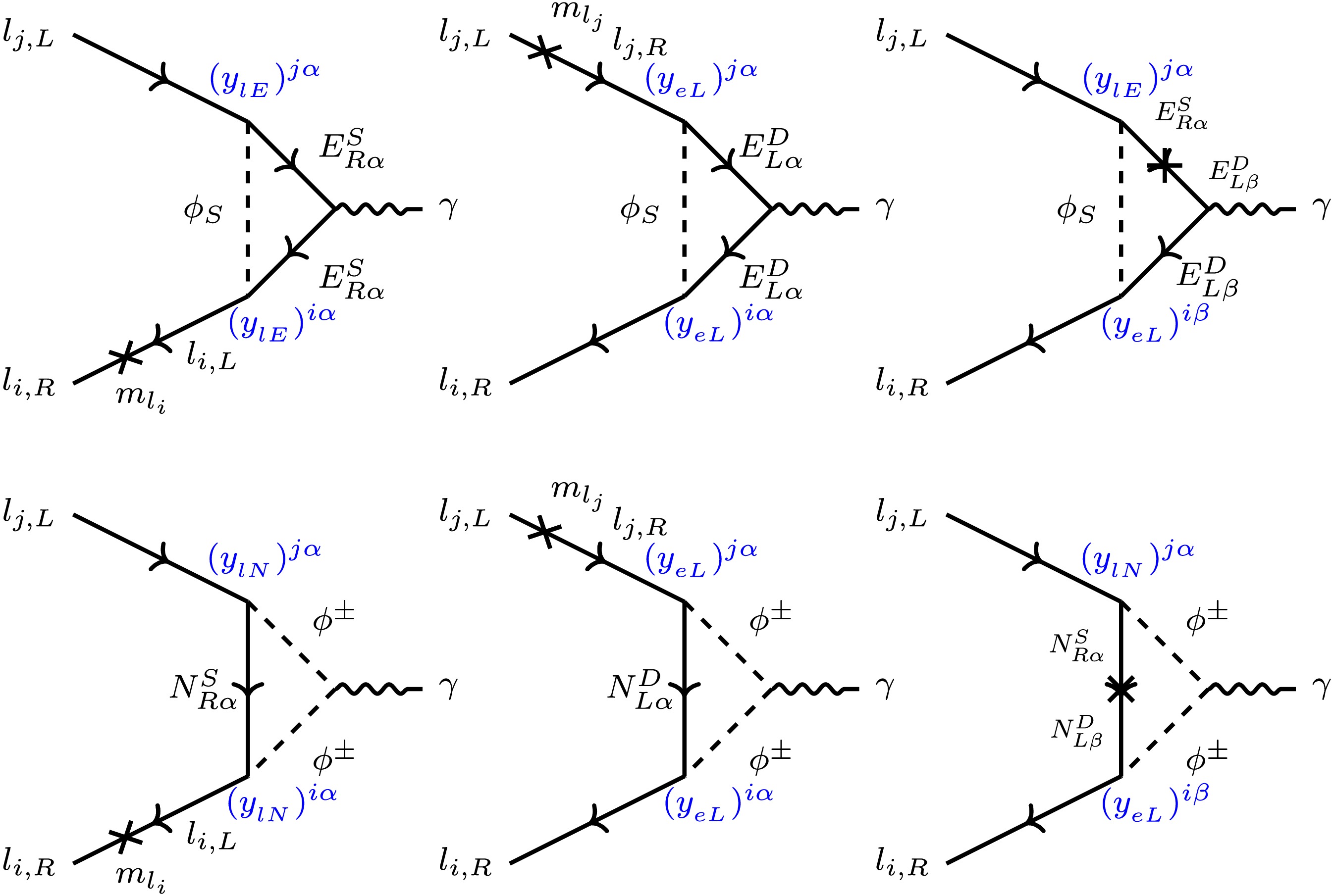
Figure 4. (color online) Feynman diagrams representing the process
$ l_{jL} \to l_{iR} \; \gamma $ , where$ i,j=1-3 $ denote the three SM charged leptons, are considered. Exotic fermions in the loop are expressed in gauge bases with indices$ \alpha, \beta=1,2 $ . This set of diagrams contributes to the matrix$ A^L_{ij} $ . The contribution to$ A^R_{ij} $ comes from the process$ l_{jR} \to l_{iL} \; \gamma $ .$ A^L = \frac{1}{32\pi^2 m_{\phi}^2} \left[C^{LL} + C^{RR} + C^{LR} + N^{LL} + N^{RR} + N^{LR}\right], $
(36) where
$ C^{LL} $ ,$ C^{RR} $ , and$ C^{LR} $ denote contributions from the four heavy$ Z_2 $ -odd charged fermions, namely$ \widetilde{\Psi}_{\tilde \kappa}^E \ni \{ \widetilde E^D_\kappa, \widetilde E^S_\kappa\} $ with$ \kappa=1,2 $ (the diagrams in the top panel of Fig. 4), whereas$ N^{LL} $ ,$ N^{RR} $ , and$ N^{LR} $ denote contributions from the six heavy$ Z_2 $ -odd neutral fermions, namely$ \widetilde{\Psi}_{R\tilde \kappa}^N \ni \{ \widetilde N^D_{a\kappa}, \widetilde N^D_{b\kappa}, \widetilde N^S_{\kappa}\} $ (the diagrams in the bottom panel of Fig. 4). The expressions for the six contributions to$ A^L $ in terms of$ Z_2 $ -odd fermion masses, mixings, and Yukawa couplings are:$ \begin{aligned}[b] C^{RR}_{ij} =\;& -{m_l}_i \left[ y_{{lE}} \left\{ U_R^{21} \, {\cal D}^f_{{ \widetilde E^D}} \left(U_R^{21}\right)^\dagger + U_R^{22} \, {\cal D}^f_{{ \widetilde E^S}} \left(U_R^{22}\right)^\dagger \right\} y_{{lE}}^\dagger\right]^{ij}, \\ C^{LL}_{ij} =\;& -\left[ y_{{eL}} \left\{ U_L^{11} \, {\cal D}^f_{{ \widetilde E^D}} \left(U_L^{11}\right)^\dagger + U_L^{12} \, {\cal D}^f_{{ \widetilde E^S}} \left(U_L^{12}\right)^\dagger \right\} y_{{eL}}^\dagger\right]^{ij} \, {m_l}_j, \\ C^{LR}_{ij} =\;& -\left[\frac{-\lambda_3 v^2}{m_{\phi_s}^2}\right] \left[ y_{{eL}} \left\{ U_L^{11} \, {\cal M}_{{ \widetilde E^D}} {\cal D}^g_{{ \widetilde E^D}} \left(U_R^{21}\right)^\dagger + U_L^{12} \, {\cal M}_{{ \widetilde E^S}} {\cal D}^g_{{ \widetilde E^S}} \left(U_R^{22}\right)^\dagger \right\} y_{{lE}}^\dagger\right]^{ij}, \\ N^{RR}_{ij} =\;& {m_l}_i \left[ y_{{lN}} \left\{ U_N^{31} \, {\cal D}^{F_1}_{{ \widetilde N^D}_a} \left(U_N^{31}\right)^\dagger + U_N^{32} \, {\cal D}^{F_1}_{{ \widetilde N^D}_b} \left(U_N^{32}\right)^\dagger + U_N^{33} \, {\cal D}^{F_1}_{\widetilde N^S} \left(U_N^{33}\right)^\dagger \right\} y_{{lN}}^\dagger\right]^{ij}, \\ N^{LL}_{ij} =\;& \left[ y_{{eL}} \left\{ \left(U_N^{11}\right)^* \, {\cal D}^{F_1}_{{ \widetilde N^D}_a} \left(U_N^{11}\right)^T + \left(U_N^{12}\right)^* \, {\cal D}^{F_1}_{{ \widetilde N^D}_b} \left(U_N^{12}\right)^T + \left(U_N^{13}\right)^* \, {\cal D}^{F_1}_{\widetilde N^S} \left(U_N^{13}\right)^T \right\} y_{{eL}}^\dagger\right]^{ij} \, {m_l}_j, \\ N^{LR}_{ij} =\;& -\left[ y_{{eL}} \left\{ \left(U_N^{11}\right)^* \, {\cal M}_{{ \widetilde N^D}_a} {\cal D}^{F_2}_{{ \widetilde N^D}_a} \left(U_N^{31}\right)^\dagger + \left(U_N^{12}\right)^* \, {\cal M}_{{ \widetilde N^D}_b} {\cal D}^{F_2}_{{ \widetilde N^D}_b} \left(U_N^{32}\right)^\dagger \right. \right. + \left. \left. \left(U_N^{13}\right)^* \, {\cal M}_{\widetilde N^S} {\cal D}^{F_2}_{\widetilde N^S} \left(U_N^{33}\right)^\dagger \right\} y_{{lN}}^\dagger\right]^{ij}, \end{aligned} $
(37) where
$ U_L^{lm} $ ,$ U_R^{lm} $ , and$ U_N^{lm} $ represent the '$ lm^{\text{th}} $ '$ 2\times 2 $ block of the$ 4\times 4 $ mixing matrices$ U_L^E $ ,$ U_R^E $ in the exotic charged fermion sector, and the$ 6\times 6 $ mixing matrix$ U_N $ in the exotic neutral fermion sector, respectively (see Eq. (12)). The matrices$ {\cal M}_Y={{\rm{Diag}}} \left[m_{Y_1}, m_{Y_2} \right] $ while$ {\cal D}^{A}_{Y}={{\rm{Diag}}} \left[A(\nu_{Y_1}), A(\nu_{Y_2}) \right] $ are defined in terms of the loop function$ A(\nu) $ with$ \nu_{Y_i}={m_{Y_i}^{2}}/{m_{\phi_S}^2} $ :$ \begin{aligned} & f(x)\; =\; F_3(x) + \frac{\lambda_3 v^2}{m_{\phi_s}^2} F_3(x) + \frac{\lambda_3 v^2}{m_{\phi_s}^2} x F_3' (x), \; \; g(x)\; =\; F_4(x) + x F_4'(x), \\ & F_1 \left( x \right)\; =\; \frac{ \left( 1-6x+3x^2+2x^3-6x^2 \ln x \right)}{6(1-x)^4}, \; \; F_2 \left( x \right)\; =\; \frac{ \left( 1-x^2+2x \ln x \right)}{(1-x)^3},\\ & F_3 \left( x \right)\; =\; \frac{ \left( 2+3x-6x^2+x^3+6x \ln x \right)}{6(1-x)^4}, \; \; F_4 \left( x \right)\; =\; \frac{ \left( -3+4x-x^2-2 \ln x \right)}{(1-x)^3}. \end{aligned} $
At this point, one should note the following:
● The elements of
$ N^{LR} $ ($ C^{LR} $ ) are enhanced by the TeV-scale masses of the$ Z_2 $ -odd neutral (charged) fermions, namely,$ m_{{ \widetilde N^D}_{a,\kappa}},\; m_{{ \widetilde N^D}_{b,\kappa}},\; {{\rm{and}}}\; m_{\widetilde N^S_{\kappa}} $ ($ m_{{ \widetilde E^D}_{\kappa}}\; {{\rm{and}}}\; m_{{ \widetilde E^S}_{\kappa}} $ ), where$ \kappa\; =\; 1,2 $ . Consequently, these contributions are orders of magnitude larger than those of$ N^{LL} $ and$ N^{RR} $ ($ C^{LL} $ and$ C^{RR} $ ), whose elements are proportional to the SM-charged lepton masses.● Eq. (37) clearly shows that
$ C^{LR} $ is proportional to$ \lambda_3 $ , while the$ \lambda_3 $ dependence of$ N^{LR} $ results from the$ \lambda_3 $ dependence of$ y_{_{lN}} $ (see Eq. (32)), which scales as$ \lambda_3^{-1/2} $ . Therefore, for large$ \lambda_3 $ , dominant contributions to cLFV and$ g-2 $ result from$ C^{LR} $ , while$ N^{LR} $ contributes dominantly for small$ \lambda_3 $ .●
$ C^{LR} $ and$ N^{LR} $ are matrices of rank 2 as the matrix product on the RHS of Eq. (37) includes a matrix of dimensions$ 2 \times 2 $ . Thus, in both the regions with either$ C^{LR} $ or$ N^{LR} $ as the dominant contributions, it is possible to address the issues of the anomalous magnetic moments of the electron as well as the muon while keeping$ {\rm Br}(\mu \to e \gamma) $ highly suppressed.● To explain the discrepancy between the observed and the SM predicted values of electron and muon
$ g-2 $ ,$ C^{LR}\sim{\cal O} \left(0.1-1 \right) $ is required (see Eq. (34)). This can be easily obtained for$ \lambda_3 \sim{\cal O} \left(1 \right) $ and$ y_{{eL}},\; y_{{lE}} \sim{\cal O} \left(1 \right) $ , with sufficiently large mixings (i.e.,$ U_{L(R)}^E\sim{\cal O} \left(0.1 \right) $ ) between the exotic fermions.● In the small
$ \lambda_3 $ region, obtaining$ N^{LR}\sim{\cal O} \left(0.1-1 \right) $ for$ y_{{eL}} \sim{\cal O} \left(1 \right) $ requires$ \lambda_3 \sim{\cal O} \left(10^{-8} \right) $ . Then,$ y_{_{lN}} \sim{\cal O} \left(10^{-3}- 10^{-1} \right) $ , and both$ \Delta a_e $ and$ \Delta a_\mu $ can be generated while keeping$ {\rm Br}(\mu \to e \gamma) $ suppressed.It may be noted here that in appropriate limits, our analytical expressions for the anomalous magnetic moments and lepton flavor violating observables reproduce the known results in the literature. In particular, when the vector-like fermion sector is suitably simplified, our results reduce to those obtained for the scotogenic model [30, 101] as well as in related frameworks like [16]. The above discussion shows that anomalous magnetic moments of both the electron and muon can be generated in the framework of the present model for
$ \lambda_3 \sim{\cal O} \left(1 \right) $ or$ {\cal O} \left(10^{-8} \right) $ . In the latter case, however, the structure of$ y_{{lN}} $ is constrained from neutrino mass generation and, therefore, in the$ N^{LR} $ contribution, a simultaneous suppression of$ {\rm Br}(\tau \to e \gamma) $ and$ {\rm Br}(\tau \to \mu \gamma) $ is not guaranteed. Furthermore, the$ N^{RR} $ (the texture of which is almost completely determined from the low energy observables in the neutrino sector) contribution to the cLFV processes is significantly enhanced for such a small$ \lambda_3 $ . As a result, we only study the large$ \lambda_3 $ region (i.e.,$ \lambda_3 \sim{\cal O} \left(1 \right) $ ) in the next part of our analysis.While the Wilson coefficients
$ A^{L(R)} $ may be computed straightforwardly in terms of the general masses and Yukawa matrices, it is instructive to consider their approximate analytical form12 in the simplified scenario:$ \begin{aligned}[b] C^{RR}&\approx-m_l\; y_{{lE}} \; \left[ f({\rho}_L) \chi_E^2 z_{{RE}}^{\dagger} z_{{RE}} + f({\rho}_E) I_{n \times n} \right]\; { y_{{lE}}}^{\dagger},\\ C^{LL}&\approx- y_{{eL}} \; \left[ f({\rho}_L) I_{n \times n} + f({\rho}_E) \chi_E^2 z_{LE} z_{LE}^{\dagger} \right]\; { y_{{eL}}}^{\dagger}m_l,\\ C^{LR}&\approx \left(\frac{\lambda_3 v^2}{m_{\phi_s}^2} \right) \; \chi_E\; y_{{eL}} \; \Big\{ \big(\widetilde{m}_E\; g({\rho}_E)-\epsilon_E \widetilde{m}_L\; g({\rho}_L)\big) z_{LE} - \big(\widetilde{m}_L\; g({\rho}_L)-\epsilon_E\widetilde{m}_E\; g({\rho}_E)\big) z_{{RE}} \Big\}\; { y_{{lE}}}^{\dagger},\end{aligned} $
$ \begin{aligned}[b] N^{RR}&\approx\frac{16 \pi^2 \widetilde m_N {\lambda}_3^{-1}}{v^2 I \left({\omega}_N \right)}\; m_l\; U_{MNS}^*\; D_{\sqrt{\nu}}\; R\; P\; R^{\dagger}\; D_{\sqrt{\nu}}\; U_{MNS}^T,\\ N^{LL}&\approx y_{{eL}} \; \left[ F_1({\rho}_L) I_{n \times n} + 2 \chi_N^2 z_{LN} z_{LN}^{\dagger} \left( F_1({\rho}_N)\; -\; F_1({\rho}_L) \right) \right]\; { y_{{eL}}}^{\dagger} m_l,\\ N^{LR}\; &\approx\frac{-4\pi}{v}\sqrt{\frac{2 \widetilde m_N}{\lambda_3 I \left({\omega}_N \right)}}\; y_{{eL}} \; \left( \; \widetilde m_N F_2({\rho}_N) - \epsilon_N \; \widetilde m_L F_2({\rho}_L) \right)\; {\chi}_N\; z_{LN}\; R^{\dagger}\; D_{\sqrt{\nu}}\; U_{MNS}^T,\end{aligned} $
(38) where
$ P=F_1({\rho}_N) I_{n \times n} + 2 \chi_N^2 z_{LN}^T z_{LN}^* \left(F_1({\rho}_L)-F_1({\rho}_N) \right) $ ,$ \rho_{L(E)[N]}= \dfrac{\widetilde m_{L(E)[N]}^2}{m_{\phi}^2} $ , and$ m_l={{\rm{diag}} \left(m_e, m_\mu, m_\tau \right)} $ is a$ 3 \times 3 $ diagonal matrix with the masses of the SM charged leptons as the diagonal entries. -
The combination of heavy neutral and charged fermions and scalars in the model gives rise to charged lepton flavor violation (cLFV) processes as well as additional contributions to
$ g-2 $ for the SM charged leptons. The effective operator resulting in cLFV decays$ l_j \to l_i \gamma $ and also contributing to the$ g-2 $ of the SM charged leptons can be expressed as$ {\cal L}_{cLFV}^{ij}\; =\; \overline{l_i}\sigma_{\mu\nu} \left( {A^L_{ij} P_L + A^R_{ij} P_R} \right) l_j F^{\mu\nu}, $
(33) where
$ P_L $ and$ P_R $ are the chirality projection operators. This leads to$ \Gamma (l_j \to l_i \gamma) = \frac{\alpha_e}{4} m_{l_j}^3 \left( |A^L_{ij}|^2 + |A^R_{ij}|^2 \right), $
(34) where kinematically allowed, and to
$ a_{l_i}=\frac{1}{2}(g_{l_i}-2)=-2\; m_{l_i}\; {{\rm{Re}}} \left( A^L_{ii} \right). $
(35) Contributions to
$ A^L $ ($ A^R $ ) result from the six Feynman diagrams depicted in Fig. 4. The exotic fermions in the loop are expressed in gauge bases. Making transformations to mass bases,$ A^L $ can be written as11 :
Figure 4. (color online) Feynman diagrams representing the process
$ l_{jL} \to l_{iR} \; \gamma $ , where$ i,j=1-3 $ denote the three SM charged leptons, are considered. Exotic fermions in the loop are expressed in gauge bases with indices$ \alpha, \beta=1,2 $ . This set of diagrams contributes to the matrix$ A^L_{ij} $ . The contribution to$ A^R_{ij} $ comes from the process$ l_{jR} \to l_{iL} \; \gamma $ .$ A^L = \frac{1}{32\pi^2 m_{\phi}^2} \left[C^{LL} + C^{RR} + C^{LR} + N^{LL} + N^{RR} + N^{LR}\right], $
(36) where
$ C^{LL} $ ,$ C^{RR} $ , and$ C^{LR} $ denote contributions from the four heavy$ Z_2 $ -odd charged fermions, namely$ \widetilde{\Psi}_{\tilde \kappa}^E \ni \{ \widetilde E^D_\kappa, \widetilde E^S_\kappa\} $ with$ \kappa=1,2 $ (the diagrams in the top panel of Fig. 4), whereas$ N^{LL} $ ,$ N^{RR} $ , and$ N^{LR} $ denote contributions from the six heavy$ Z_2 $ -odd neutral fermions, namely$ \widetilde{\Psi}_{R\tilde \kappa}^N \ni \{ \widetilde N^D_{a\kappa}, \widetilde N^D_{b\kappa}, \widetilde N^S_{\kappa}\} $ (the diagrams in the bottom panel of Fig. 4). The expressions for the six contributions to$ A^L $ in terms of$ Z_2 $ -odd fermion masses, mixings, and Yukawa couplings are:$ \begin{aligned}[b] C^{RR}_{ij} =\;& -{m_l}_i \left[ y_{{lE}} \left\{ U_R^{21} \, {\cal D}^f_{{ \widetilde E^D}} \left(U_R^{21}\right)^\dagger + U_R^{22} \, {\cal D}^f_{{ \widetilde E^S}} \left(U_R^{22}\right)^\dagger \right\} y_{{lE}}^\dagger\right]^{ij}, \\ C^{LL}_{ij} =\;& -\left[ y_{{eL}} \left\{ U_L^{11} \, {\cal D}^f_{{ \widetilde E^D}} \left(U_L^{11}\right)^\dagger + U_L^{12} \, {\cal D}^f_{{ \widetilde E^S}} \left(U_L^{12}\right)^\dagger \right\} y_{{eL}}^\dagger\right]^{ij} \, {m_l}_j, \\ C^{LR}_{ij} =\;& -\left[\frac{-\lambda_3 v^2}{m_{\phi_s}^2}\right] \left[ y_{{eL}} \left\{ U_L^{11} \, {\cal M}_{{ \widetilde E^D}} {\cal D}^g_{{ \widetilde E^D}} \left(U_R^{21}\right)^\dagger + U_L^{12} \, {\cal M}_{{ \widetilde E^S}} {\cal D}^g_{{ \widetilde E^S}} \left(U_R^{22}\right)^\dagger \right\} y_{{lE}}^\dagger\right]^{ij}, \\ N^{RR}_{ij} =\;& {m_l}_i \left[ y_{{lN}} \left\{ U_N^{31} \, {\cal D}^{F_1}_{{ \widetilde N^D}_a} \left(U_N^{31}\right)^\dagger + U_N^{32} \, {\cal D}^{F_1}_{{ \widetilde N^D}_b} \left(U_N^{32}\right)^\dagger + U_N^{33} \, {\cal D}^{F_1}_{\widetilde N^S} \left(U_N^{33}\right)^\dagger \right\} y_{{lN}}^\dagger\right]^{ij}, \\ N^{LL}_{ij} =\;& \left[ y_{{eL}} \left\{ \left(U_N^{11}\right)^* \, {\cal D}^{F_1}_{{ \widetilde N^D}_a} \left(U_N^{11}\right)^T + \left(U_N^{12}\right)^* \, {\cal D}^{F_1}_{{ \widetilde N^D}_b} \left(U_N^{12}\right)^T + \left(U_N^{13}\right)^* \, {\cal D}^{F_1}_{\widetilde N^S} \left(U_N^{13}\right)^T \right\} y_{{eL}}^\dagger\right]^{ij} \, {m_l}_j, \\ N^{LR}_{ij} =\;& -\left[ y_{{eL}} \left\{ \left(U_N^{11}\right)^* \, {\cal M}_{{ \widetilde N^D}_a} {\cal D}^{F_2}_{{ \widetilde N^D}_a} \left(U_N^{31}\right)^\dagger + \left(U_N^{12}\right)^* \, {\cal M}_{{ \widetilde N^D}_b} {\cal D}^{F_2}_{{ \widetilde N^D}_b} \left(U_N^{32}\right)^\dagger \right. \right. + \left. \left. \left(U_N^{13}\right)^* \, {\cal M}_{\widetilde N^S} {\cal D}^{F_2}_{\widetilde N^S} \left(U_N^{33}\right)^\dagger \right\} y_{{lN}}^\dagger\right]^{ij}, \end{aligned} $
(37) where
$ U_L^{lm} $ ,$ U_R^{lm} $ , and$ U_N^{lm} $ represent the '$ lm^{\text{th}} $ '$ 2\times 2 $ block of the$ 4\times 4 $ mixing matrices$ U_L^E $ ,$ U_R^E $ in the exotic charged fermion sector, and the$ 6\times 6 $ mixing matrix$ U_N $ in the exotic neutral fermion sector, respectively (see Eq. (12)). The matrices$ {\cal M}_Y={{\rm{Diag}}} \left[m_{Y_1}, m_{Y_2} \right] $ while$ {\cal D}^{A}_{Y}={{\rm{Diag}}} \left[A(\nu_{Y_1}), A(\nu_{Y_2}) \right] $ are defined in terms of the loop function$ A(\nu) $ with$ \nu_{Y_i}={m_{Y_i}^{2}}/{m_{\phi_S}^2} $ :$ \begin{aligned} & f(x)\; =\; F_3(x) + \frac{\lambda_3 v^2}{m_{\phi_s}^2} F_3(x) + \frac{\lambda_3 v^2}{m_{\phi_s}^2} x F_3' (x), \; \; g(x)\; =\; F_4(x) + x F_4'(x), \\ & F_1 \left( x \right)\; =\; \frac{ \left( 1-6x+3x^2+2x^3-6x^2 \ln x \right)}{6(1-x)^4}, \; \; F_2 \left( x \right)\; =\; \frac{ \left( 1-x^2+2x \ln x \right)}{(1-x)^3},\\ & F_3 \left( x \right)\; =\; \frac{ \left( 2+3x-6x^2+x^3+6x \ln x \right)}{6(1-x)^4}, \; \; F_4 \left( x \right)\; =\; \frac{ \left( -3+4x-x^2-2 \ln x \right)}{(1-x)^3}. \end{aligned} $
At this point, one should note the following:
● The elements of
$ N^{LR} $ ($ C^{LR} $ ) are enhanced by the TeV-scale masses of the$ Z_2 $ -odd neutral (charged) fermions, namely,$ m_{{ \widetilde N^D}_{a,\kappa}},\; m_{{ \widetilde N^D}_{b,\kappa}},\; {{\rm{and}}}\; m_{\widetilde N^S_{\kappa}} $ ($ m_{{ \widetilde E^D}_{\kappa}}\; {{\rm{and}}}\; m_{{ \widetilde E^S}_{\kappa}} $ ), where$ \kappa\; =\; 1,2 $ . Consequently, these contributions are orders of magnitude larger than those of$ N^{LL} $ and$ N^{RR} $ ($ C^{LL} $ and$ C^{RR} $ ), whose elements are proportional to the SM-charged lepton masses.● Eq. (37) clearly shows that
$ C^{LR} $ is proportional to$ \lambda_3 $ , while the$ \lambda_3 $ dependence of$ N^{LR} $ results from the$ \lambda_3 $ dependence of$ y_{_{lN}} $ (see Eq. (32)), which scales as$ \lambda_3^{-1/2} $ . Therefore, for large$ \lambda_3 $ , dominant contributions to cLFV and$ g-2 $ result from$ C^{LR} $ , while$ N^{LR} $ contributes dominantly for small$ \lambda_3 $ .●
$ C^{LR} $ and$ N^{LR} $ are matrices of rank 2 as the matrix product on the RHS of Eq. (37) includes a matrix of dimensions$ 2 \times 2 $ . Thus, in both the regions with either$ C^{LR} $ or$ N^{LR} $ as the dominant contributions, it is possible to address the issues of the anomalous magnetic moments of the electron as well as the muon while keeping$ {\rm Br}(\mu \to e \gamma) $ highly suppressed.● To explain the discrepancy between the observed and the SM predicted values of electron and muon
$ g-2 $ ,$ C^{LR}\sim{\cal O} \left(0.1-1 \right) $ is required (see Eq. (34)). This can be easily obtained for$ \lambda_3 \sim{\cal O} \left(1 \right) $ and$ y_{{eL}},\; y_{{lE}} \sim{\cal O} \left(1 \right) $ , with sufficiently large mixings (i.e.,$ U_{L(R)}^E\sim{\cal O} \left(0.1 \right) $ ) between the exotic fermions.● In the small
$ \lambda_3 $ region, obtaining$ N^{LR}\sim{\cal O} \left(0.1-1 \right) $ for$ y_{{eL}} \sim{\cal O} \left(1 \right) $ requires$ \lambda_3 \sim{\cal O} \left(10^{-8} \right) $ . Then,$ y_{_{lN}} \sim{\cal O} \left(10^{-3}- 10^{-1} \right) $ , and both$ \Delta a_e $ and$ \Delta a_\mu $ can be generated while keeping$ {\rm Br}(\mu \to e \gamma) $ suppressed.It may be noted here that in appropriate limits, our analytical expressions for the anomalous magnetic moments and lepton flavor violating observables reproduce the known results in the literature. In particular, when the vector-like fermion sector is suitably simplified, our results reduce to those obtained for the scotogenic model [30, 101] as well as in related frameworks like [16]. The above discussion shows that anomalous magnetic moments of both the electron and muon can be generated in the framework of the present model for
$ \lambda_3 \sim{\cal O} \left(1 \right) $ or$ {\cal O} \left(10^{-8} \right) $ . In the latter case, however, the structure of$ y_{{lN}} $ is constrained from neutrino mass generation and, therefore, in the$ N^{LR} $ contribution, a simultaneous suppression of$ {\rm Br}(\tau \to e \gamma) $ and$ {\rm Br}(\tau \to \mu \gamma) $ is not guaranteed. Furthermore, the$ N^{RR} $ (the texture of which is almost completely determined from the low energy observables in the neutrino sector) contribution to the cLFV processes is significantly enhanced for such a small$ \lambda_3 $ . As a result, we only study the large$ \lambda_3 $ region (i.e.,$ \lambda_3 \sim{\cal O} \left(1 \right) $ ) in the next part of our analysis.While the Wilson coefficients
$ A^{L(R)} $ may be computed straightforwardly in terms of the general masses and Yukawa matrices, it is instructive to consider their approximate analytical form12 in the simplified scenario:$ \begin{aligned}[b] C^{RR}&\approx-m_l\; y_{{lE}} \; \left[ f({\rho}_L) \chi_E^2 z_{{RE}}^{\dagger} z_{{RE}} + f({\rho}_E) I_{n \times n} \right]\; { y_{{lE}}}^{\dagger},\\ C^{LL}&\approx- y_{{eL}} \; \left[ f({\rho}_L) I_{n \times n} + f({\rho}_E) \chi_E^2 z_{LE} z_{LE}^{\dagger} \right]\; { y_{{eL}}}^{\dagger}m_l,\\ C^{LR}&\approx \left(\frac{\lambda_3 v^2}{m_{\phi_s}^2} \right) \; \chi_E\; y_{{eL}} \; \Big\{ \big(\widetilde{m}_E\; g({\rho}_E)-\epsilon_E \widetilde{m}_L\; g({\rho}_L)\big) z_{LE} - \big(\widetilde{m}_L\; g({\rho}_L)-\epsilon_E\widetilde{m}_E\; g({\rho}_E)\big) z_{{RE}} \Big\}\; { y_{{lE}}}^{\dagger},\end{aligned} $
$ \begin{aligned}[b] N^{RR}&\approx\frac{16 \pi^2 \widetilde m_N {\lambda}_3^{-1}}{v^2 I \left({\omega}_N \right)}\; m_l\; U_{MNS}^*\; D_{\sqrt{\nu}}\; R\; P\; R^{\dagger}\; D_{\sqrt{\nu}}\; U_{MNS}^T,\\ N^{LL}&\approx y_{{eL}} \; \left[ F_1({\rho}_L) I_{n \times n} + 2 \chi_N^2 z_{LN} z_{LN}^{\dagger} \left( F_1({\rho}_N)\; -\; F_1({\rho}_L) \right) \right]\; { y_{{eL}}}^{\dagger} m_l,\\ N^{LR}\; &\approx\frac{-4\pi}{v}\sqrt{\frac{2 \widetilde m_N}{\lambda_3 I \left({\omega}_N \right)}}\; y_{{eL}} \; \left( \; \widetilde m_N F_2({\rho}_N) - \epsilon_N \; \widetilde m_L F_2({\rho}_L) \right)\; {\chi}_N\; z_{LN}\; R^{\dagger}\; D_{\sqrt{\nu}}\; U_{MNS}^T,\end{aligned} $
(38) where
$ P=F_1({\rho}_N) I_{n \times n} + 2 \chi_N^2 z_{LN}^T z_{LN}^* \left(F_1({\rho}_L)-F_1({\rho}_N) \right) $ ,$ \rho_{L(E)[N]}= \dfrac{\widetilde m_{L(E)[N]}^2}{m_{\phi}^2} $ , and$ m_l={{\rm{diag}} \left(m_e, m_\mu, m_\tau \right)} $ is a$ 3 \times 3 $ diagonal matrix with the masses of the SM charged leptons as the diagonal entries. -
The combination of heavy neutral and charged fermions and scalars in the model gives rise to charged lepton flavor violation (cLFV) processes as well as additional contributions to
$ g-2 $ for the SM charged leptons. The effective operator resulting in cLFV decays$ l_j \to l_i \gamma $ and also contributing to the$ g-2 $ of the SM charged leptons can be expressed as$ {\cal L}_{cLFV}^{ij}\; =\; \overline{l_i}\sigma_{\mu\nu} \left( {A^L_{ij} P_L + A^R_{ij} P_R} \right) l_j F^{\mu\nu}, $
(33) where
$ P_L $ and$ P_R $ are the chirality projection operators. This leads to$ \Gamma (l_j \to l_i \gamma) = \frac{\alpha_e}{4} m_{l_j}^3 \left( |A^L_{ij}|^2 + |A^R_{ij}|^2 \right), $
(34) where kinematically allowed, and to
$ a_{l_i}=\frac{1}{2}(g_{l_i}-2)=-2\; m_{l_i}\; {{\rm{Re}}} \left( A^L_{ii} \right). $
(35) Contributions to
$ A^L $ ($ A^R $ ) result from the six Feynman diagrams depicted in Fig. 4. The exotic fermions in the loop are expressed in gauge bases. Making transformations to mass bases,$ A^L $ can be written as11 :
Figure 4. (color online) Feynman diagrams representing the process
$ l_{jL} \to l_{iR} \; \gamma $ , where$ i,j=1-3 $ denote the three SM charged leptons, are considered. Exotic fermions in the loop are expressed in gauge bases with indices$ \alpha, \beta=1,2 $ . This set of diagrams contributes to the matrix$ A^L_{ij} $ . The contribution to$ A^R_{ij} $ comes from the process$ l_{jR} \to l_{iL} \; \gamma $ .$ A^L = \frac{1}{32\pi^2 m_{\phi}^2} \left[C^{LL} + C^{RR} + C^{LR} + N^{LL} + N^{RR} + N^{LR}\right], $
(36) where
$ C^{LL} $ ,$ C^{RR} $ , and$ C^{LR} $ denote contributions from the four heavy$ Z_2 $ -odd charged fermions, namely$ \widetilde{\Psi}_{\tilde \kappa}^E \ni \{ \widetilde E^D_\kappa, \widetilde E^S_\kappa\} $ with$ \kappa=1,2 $ (the diagrams in the top panel of Fig. 4), whereas$ N^{LL} $ ,$ N^{RR} $ , and$ N^{LR} $ denote contributions from the six heavy$ Z_2 $ -odd neutral fermions, namely$ \widetilde{\Psi}_{R\tilde \kappa}^N \ni \{ \widetilde N^D_{a\kappa}, \widetilde N^D_{b\kappa}, \widetilde N^S_{\kappa}\} $ (the diagrams in the bottom panel of Fig. 4). The expressions for the six contributions to$ A^L $ in terms of$ Z_2 $ -odd fermion masses, mixings, and Yukawa couplings are:$ \begin{aligned}[b] C^{RR}_{ij} =\;& -{m_l}_i \left[ y_{{lE}} \left\{ U_R^{21} \, {\cal D}^f_{{ \widetilde E^D}} \left(U_R^{21}\right)^\dagger + U_R^{22} \, {\cal D}^f_{{ \widetilde E^S}} \left(U_R^{22}\right)^\dagger \right\} y_{{lE}}^\dagger\right]^{ij}, \\ C^{LL}_{ij} =\;& -\left[ y_{{eL}} \left\{ U_L^{11} \, {\cal D}^f_{{ \widetilde E^D}} \left(U_L^{11}\right)^\dagger + U_L^{12} \, {\cal D}^f_{{ \widetilde E^S}} \left(U_L^{12}\right)^\dagger \right\} y_{{eL}}^\dagger\right]^{ij} \, {m_l}_j, \\ C^{LR}_{ij} =\;& -\left[\frac{-\lambda_3 v^2}{m_{\phi_s}^2}\right] \left[ y_{{eL}} \left\{ U_L^{11} \, {\cal M}_{{ \widetilde E^D}} {\cal D}^g_{{ \widetilde E^D}} \left(U_R^{21}\right)^\dagger + U_L^{12} \, {\cal M}_{{ \widetilde E^S}} {\cal D}^g_{{ \widetilde E^S}} \left(U_R^{22}\right)^\dagger \right\} y_{{lE}}^\dagger\right]^{ij}, \\ N^{RR}_{ij} =\;& {m_l}_i \left[ y_{{lN}} \left\{ U_N^{31} \, {\cal D}^{F_1}_{{ \widetilde N^D}_a} \left(U_N^{31}\right)^\dagger + U_N^{32} \, {\cal D}^{F_1}_{{ \widetilde N^D}_b} \left(U_N^{32}\right)^\dagger + U_N^{33} \, {\cal D}^{F_1}_{\widetilde N^S} \left(U_N^{33}\right)^\dagger \right\} y_{{lN}}^\dagger\right]^{ij}, \\ N^{LL}_{ij} =\;& \left[ y_{{eL}} \left\{ \left(U_N^{11}\right)^* \, {\cal D}^{F_1}_{{ \widetilde N^D}_a} \left(U_N^{11}\right)^T + \left(U_N^{12}\right)^* \, {\cal D}^{F_1}_{{ \widetilde N^D}_b} \left(U_N^{12}\right)^T + \left(U_N^{13}\right)^* \, {\cal D}^{F_1}_{\widetilde N^S} \left(U_N^{13}\right)^T \right\} y_{{eL}}^\dagger\right]^{ij} \, {m_l}_j, \\ N^{LR}_{ij} =\;& -\left[ y_{{eL}} \left\{ \left(U_N^{11}\right)^* \, {\cal M}_{{ \widetilde N^D}_a} {\cal D}^{F_2}_{{ \widetilde N^D}_a} \left(U_N^{31}\right)^\dagger + \left(U_N^{12}\right)^* \, {\cal M}_{{ \widetilde N^D}_b} {\cal D}^{F_2}_{{ \widetilde N^D}_b} \left(U_N^{32}\right)^\dagger \right. \right. + \left. \left. \left(U_N^{13}\right)^* \, {\cal M}_{\widetilde N^S} {\cal D}^{F_2}_{\widetilde N^S} \left(U_N^{33}\right)^\dagger \right\} y_{{lN}}^\dagger\right]^{ij}, \end{aligned} $
(37) where
$ U_L^{lm} $ ,$ U_R^{lm} $ , and$ U_N^{lm} $ represent the '$ lm^{\text{th}} $ '$ 2\times 2 $ block of the$ 4\times 4 $ mixing matrices$ U_L^E $ ,$ U_R^E $ in the exotic charged fermion sector, and the$ 6\times 6 $ mixing matrix$ U_N $ in the exotic neutral fermion sector, respectively (see Eq. (12)). The matrices$ {\cal M}_Y={{\rm{Diag}}} \left[m_{Y_1}, m_{Y_2} \right] $ while$ {\cal D}^{A}_{Y}={{\rm{Diag}}} \left[A(\nu_{Y_1}), A(\nu_{Y_2}) \right] $ are defined in terms of the loop function$ A(\nu) $ with$ \nu_{Y_i}={m_{Y_i}^{2}}/{m_{\phi_S}^2} $ :$ \begin{aligned} & f(x)\; =\; F_3(x) + \frac{\lambda_3 v^2}{m_{\phi_s}^2} F_3(x) + \frac{\lambda_3 v^2}{m_{\phi_s}^2} x F_3' (x), \; \; g(x)\; =\; F_4(x) + x F_4'(x), \\ & F_1 \left( x \right)\; =\; \frac{ \left( 1-6x+3x^2+2x^3-6x^2 \ln x \right)}{6(1-x)^4}, \; \; F_2 \left( x \right)\; =\; \frac{ \left( 1-x^2+2x \ln x \right)}{(1-x)^3},\\ & F_3 \left( x \right)\; =\; \frac{ \left( 2+3x-6x^2+x^3+6x \ln x \right)}{6(1-x)^4}, \; \; F_4 \left( x \right)\; =\; \frac{ \left( -3+4x-x^2-2 \ln x \right)}{(1-x)^3}. \end{aligned} $
At this point, one should note the following:
● The elements of
$ N^{LR} $ ($ C^{LR} $ ) are enhanced by the TeV-scale masses of the$ Z_2 $ -odd neutral (charged) fermions, namely,$ m_{{ \widetilde N^D}_{a,\kappa}},\; m_{{ \widetilde N^D}_{b,\kappa}},\; {{\rm{and}}}\; m_{\widetilde N^S_{\kappa}} $ ($ m_{{ \widetilde E^D}_{\kappa}}\; {{\rm{and}}}\; m_{{ \widetilde E^S}_{\kappa}} $ ), where$ \kappa\; =\; 1,2 $ . Consequently, these contributions are orders of magnitude larger than those of$ N^{LL} $ and$ N^{RR} $ ($ C^{LL} $ and$ C^{RR} $ ), whose elements are proportional to the SM-charged lepton masses.● Eq. (37) clearly shows that
$ C^{LR} $ is proportional to$ \lambda_3 $ , while the$ \lambda_3 $ dependence of$ N^{LR} $ results from the$ \lambda_3 $ dependence of$ y_{_{lN}} $ (see Eq. (32)), which scales as$ \lambda_3^{-1/2} $ . Therefore, for large$ \lambda_3 $ , dominant contributions to cLFV and$ g-2 $ result from$ C^{LR} $ , while$ N^{LR} $ contributes dominantly for small$ \lambda_3 $ .●
$ C^{LR} $ and$ N^{LR} $ are matrices of rank 2 as the matrix product on the RHS of Eq. (37) includes a matrix of dimensions$ 2 \times 2 $ . Thus, in both the regions with either$ C^{LR} $ or$ N^{LR} $ as the dominant contributions, it is possible to address the issues of the anomalous magnetic moments of the electron as well as the muon while keeping$ {\rm Br}(\mu \to e \gamma) $ highly suppressed.● To explain the discrepancy between the observed and the SM predicted values of electron and muon
$ g-2 $ ,$ C^{LR}\sim{\cal O} \left(0.1-1 \right) $ is required (see Eq. (34)). This can be easily obtained for$ \lambda_3 \sim{\cal O} \left(1 \right) $ and$ y_{{eL}},\; y_{{lE}} \sim{\cal O} \left(1 \right) $ , with sufficiently large mixings (i.e.,$ U_{L(R)}^E\sim{\cal O} \left(0.1 \right) $ ) between the exotic fermions.● In the small
$ \lambda_3 $ region, obtaining$ N^{LR}\sim{\cal O} \left(0.1-1 \right) $ for$ y_{{eL}} \sim{\cal O} \left(1 \right) $ requires$ \lambda_3 \sim{\cal O} \left(10^{-8} \right) $ . Then,$ y_{_{lN}} \sim{\cal O} \left(10^{-3}- 10^{-1} \right) $ , and both$ \Delta a_e $ and$ \Delta a_\mu $ can be generated while keeping$ {\rm Br}(\mu \to e \gamma) $ suppressed.It may be noted here that in appropriate limits, our analytical expressions for the anomalous magnetic moments and lepton flavor violating observables reproduce the known results in the literature. In particular, when the vector-like fermion sector is suitably simplified, our results reduce to those obtained for the scotogenic model [30, 101] as well as in related frameworks like [16]. The above discussion shows that anomalous magnetic moments of both the electron and muon can be generated in the framework of the present model for
$ \lambda_3 \sim{\cal O} \left(1 \right) $ or$ {\cal O} \left(10^{-8} \right) $ . In the latter case, however, the structure of$ y_{{lN}} $ is constrained from neutrino mass generation and, therefore, in the$ N^{LR} $ contribution, a simultaneous suppression of$ {\rm Br}(\tau \to e \gamma) $ and$ {\rm Br}(\tau \to \mu \gamma) $ is not guaranteed. Furthermore, the$ N^{RR} $ (the texture of which is almost completely determined from the low energy observables in the neutrino sector) contribution to the cLFV processes is significantly enhanced for such a small$ \lambda_3 $ . As a result, we only study the large$ \lambda_3 $ region (i.e.,$ \lambda_3 \sim{\cal O} \left(1 \right) $ ) in the next part of our analysis.While the Wilson coefficients
$ A^{L(R)} $ may be computed straightforwardly in terms of the general masses and Yukawa matrices, it is instructive to consider their approximate analytical form12 in the simplified scenario:$ \begin{aligned}[b] C^{RR}&\approx-m_l\; y_{{lE}} \; \left[ f({\rho}_L) \chi_E^2 z_{{RE}}^{\dagger} z_{{RE}} + f({\rho}_E) I_{n \times n} \right]\; { y_{{lE}}}^{\dagger},\\ C^{LL}&\approx- y_{{eL}} \; \left[ f({\rho}_L) I_{n \times n} + f({\rho}_E) \chi_E^2 z_{LE} z_{LE}^{\dagger} \right]\; { y_{{eL}}}^{\dagger}m_l,\\ C^{LR}&\approx \left(\frac{\lambda_3 v^2}{m_{\phi_s}^2} \right) \; \chi_E\; y_{{eL}} \; \Big\{ \big(\widetilde{m}_E\; g({\rho}_E)-\epsilon_E \widetilde{m}_L\; g({\rho}_L)\big) z_{LE} - \big(\widetilde{m}_L\; g({\rho}_L)-\epsilon_E\widetilde{m}_E\; g({\rho}_E)\big) z_{{RE}} \Big\}\; { y_{{lE}}}^{\dagger},\end{aligned} $
$ \begin{aligned}[b] N^{RR}&\approx\frac{16 \pi^2 \widetilde m_N {\lambda}_3^{-1}}{v^2 I \left({\omega}_N \right)}\; m_l\; U_{MNS}^*\; D_{\sqrt{\nu}}\; R\; P\; R^{\dagger}\; D_{\sqrt{\nu}}\; U_{MNS}^T,\\ N^{LL}&\approx y_{{eL}} \; \left[ F_1({\rho}_L) I_{n \times n} + 2 \chi_N^2 z_{LN} z_{LN}^{\dagger} \left( F_1({\rho}_N)\; -\; F_1({\rho}_L) \right) \right]\; { y_{{eL}}}^{\dagger} m_l,\\ N^{LR}\; &\approx\frac{-4\pi}{v}\sqrt{\frac{2 \widetilde m_N}{\lambda_3 I \left({\omega}_N \right)}}\; y_{{eL}} \; \left( \; \widetilde m_N F_2({\rho}_N) - \epsilon_N \; \widetilde m_L F_2({\rho}_L) \right)\; {\chi}_N\; z_{LN}\; R^{\dagger}\; D_{\sqrt{\nu}}\; U_{MNS}^T,\end{aligned} $
(38) where
$ P=F_1({\rho}_N) I_{n \times n} + 2 \chi_N^2 z_{LN}^T z_{LN}^* \left(F_1({\rho}_L)-F_1({\rho}_N) \right) $ ,$ \rho_{L(E)[N]}= \dfrac{\widetilde m_{L(E)[N]}^2}{m_{\phi}^2} $ , and$ m_l={{\rm{diag}} \left(m_e, m_\mu, m_\tau \right)} $ is a$ 3 \times 3 $ diagonal matrix with the masses of the SM charged leptons as the diagonal entries. -
The combination of heavy neutral and charged fermions and scalars in the model gives rise to charged lepton flavor violation (cLFV) processes as well as additional contributions to
$ g-2 $ for the SM charged leptons. The effective operator resulting in cLFV decays$ l_j \to l_i \gamma $ and also contributing to the$ g-2 $ of the SM charged leptons can be expressed as$ {\cal L}_{cLFV}^{ij}\; =\; \overline{l_i}\sigma_{\mu\nu} \left( {A^L_{ij} P_L + A^R_{ij} P_R} \right) l_j F^{\mu\nu}, $
(33) where
$ P_L $ and$ P_R $ are the chirality projection operators. This leads to$ \Gamma (l_j \to l_i \gamma) = \frac{\alpha_e}{4} m_{l_j}^3 \left( |A^L_{ij}|^2 + |A^R_{ij}|^2 \right), $
(34) where kinematically allowed, and to
$ a_{l_i}=\frac{1}{2}(g_{l_i}-2)=-2\; m_{l_i}\; {{\rm{Re}}} \left( A^L_{ii} \right). $
(35) Contributions to
$ A^L $ ($ A^R $ ) result from the six Feynman diagrams depicted in Fig. 4. The exotic fermions in the loop are expressed in gauge bases. Making transformations to mass bases,$ A^L $ can be written as11 :
Figure 4. (color online) Feynman diagrams representing the process
$ l_{jL} \to l_{iR} \; \gamma $ , where$ i,j=1-3 $ denote the three SM charged leptons, are considered. Exotic fermions in the loop are expressed in gauge bases with indices$ \alpha, \beta=1,2 $ . This set of diagrams contributes to the matrix$ A^L_{ij} $ . The contribution to$ A^R_{ij} $ comes from the process$ l_{jR} \to l_{iL} \; \gamma $ .$ A^L = \frac{1}{32\pi^2 m_{\phi}^2} \left[C^{LL} + C^{RR} + C^{LR} + N^{LL} + N^{RR} + N^{LR}\right], $
(36) where
$ C^{LL} $ ,$ C^{RR} $ , and$ C^{LR} $ denote contributions from the four heavy$ Z_2 $ -odd charged fermions, namely$ \widetilde{\Psi}_{\tilde \kappa}^E \ni \{ \widetilde E^D_\kappa, \widetilde E^S_\kappa\} $ with$ \kappa=1,2 $ (the diagrams in the top panel of Fig. 4), whereas$ N^{LL} $ ,$ N^{RR} $ , and$ N^{LR} $ denote contributions from the six heavy$ Z_2 $ -odd neutral fermions, namely$ \widetilde{\Psi}_{R\tilde \kappa}^N \ni \{ \widetilde N^D_{a\kappa}, \widetilde N^D_{b\kappa}, \widetilde N^S_{\kappa}\} $ (the diagrams in the bottom panel of Fig. 4). The expressions for the six contributions to$ A^L $ in terms of$ Z_2 $ -odd fermion masses, mixings, and Yukawa couplings are:$ \begin{aligned}[b] C^{RR}_{ij} =\;& -{m_l}_i \left[ y_{{lE}} \left\{ U_R^{21} \, {\cal D}^f_{{ \widetilde E^D}} \left(U_R^{21}\right)^\dagger + U_R^{22} \, {\cal D}^f_{{ \widetilde E^S}} \left(U_R^{22}\right)^\dagger \right\} y_{{lE}}^\dagger\right]^{ij}, \\ C^{LL}_{ij} =\;& -\left[ y_{{eL}} \left\{ U_L^{11} \, {\cal D}^f_{{ \widetilde E^D}} \left(U_L^{11}\right)^\dagger + U_L^{12} \, {\cal D}^f_{{ \widetilde E^S}} \left(U_L^{12}\right)^\dagger \right\} y_{{eL}}^\dagger\right]^{ij} \, {m_l}_j, \\ C^{LR}_{ij} =\;& -\left[\frac{-\lambda_3 v^2}{m_{\phi_s}^2}\right] \left[ y_{{eL}} \left\{ U_L^{11} \, {\cal M}_{{ \widetilde E^D}} {\cal D}^g_{{ \widetilde E^D}} \left(U_R^{21}\right)^\dagger + U_L^{12} \, {\cal M}_{{ \widetilde E^S}} {\cal D}^g_{{ \widetilde E^S}} \left(U_R^{22}\right)^\dagger \right\} y_{{lE}}^\dagger\right]^{ij}, \\ N^{RR}_{ij} =\;& {m_l}_i \left[ y_{{lN}} \left\{ U_N^{31} \, {\cal D}^{F_1}_{{ \widetilde N^D}_a} \left(U_N^{31}\right)^\dagger + U_N^{32} \, {\cal D}^{F_1}_{{ \widetilde N^D}_b} \left(U_N^{32}\right)^\dagger + U_N^{33} \, {\cal D}^{F_1}_{\widetilde N^S} \left(U_N^{33}\right)^\dagger \right\} y_{{lN}}^\dagger\right]^{ij}, \\ N^{LL}_{ij} =\;& \left[ y_{{eL}} \left\{ \left(U_N^{11}\right)^* \, {\cal D}^{F_1}_{{ \widetilde N^D}_a} \left(U_N^{11}\right)^T + \left(U_N^{12}\right)^* \, {\cal D}^{F_1}_{{ \widetilde N^D}_b} \left(U_N^{12}\right)^T + \left(U_N^{13}\right)^* \, {\cal D}^{F_1}_{\widetilde N^S} \left(U_N^{13}\right)^T \right\} y_{{eL}}^\dagger\right]^{ij} \, {m_l}_j, \\ N^{LR}_{ij} =\;& -\left[ y_{{eL}} \left\{ \left(U_N^{11}\right)^* \, {\cal M}_{{ \widetilde N^D}_a} {\cal D}^{F_2}_{{ \widetilde N^D}_a} \left(U_N^{31}\right)^\dagger + \left(U_N^{12}\right)^* \, {\cal M}_{{ \widetilde N^D}_b} {\cal D}^{F_2}_{{ \widetilde N^D}_b} \left(U_N^{32}\right)^\dagger \right. \right. + \left. \left. \left(U_N^{13}\right)^* \, {\cal M}_{\widetilde N^S} {\cal D}^{F_2}_{\widetilde N^S} \left(U_N^{33}\right)^\dagger \right\} y_{{lN}}^\dagger\right]^{ij}, \end{aligned} $
(37) where
$ U_L^{lm} $ ,$ U_R^{lm} $ , and$ U_N^{lm} $ represent the '$ lm^{\text{th}} $ '$ 2\times 2 $ block of the$ 4\times 4 $ mixing matrices$ U_L^E $ ,$ U_R^E $ in the exotic charged fermion sector, and the$ 6\times 6 $ mixing matrix$ U_N $ in the exotic neutral fermion sector, respectively (see Eq. (12)). The matrices$ {\cal M}_Y={{\rm{Diag}}} \left[m_{Y_1}, m_{Y_2} \right] $ while$ {\cal D}^{A}_{Y}={{\rm{Diag}}} \left[A(\nu_{Y_1}), A(\nu_{Y_2}) \right] $ are defined in terms of the loop function$ A(\nu) $ with$ \nu_{Y_i}={m_{Y_i}^{2}}/{m_{\phi_S}^2} $ :$ \begin{aligned} & f(x)\; =\; F_3(x) + \frac{\lambda_3 v^2}{m_{\phi_s}^2} F_3(x) + \frac{\lambda_3 v^2}{m_{\phi_s}^2} x F_3' (x), \; \; g(x)\; =\; F_4(x) + x F_4'(x), \\ & F_1 \left( x \right)\; =\; \frac{ \left( 1-6x+3x^2+2x^3-6x^2 \ln x \right)}{6(1-x)^4}, \; \; F_2 \left( x \right)\; =\; \frac{ \left( 1-x^2+2x \ln x \right)}{(1-x)^3},\\ & F_3 \left( x \right)\; =\; \frac{ \left( 2+3x-6x^2+x^3+6x \ln x \right)}{6(1-x)^4}, \; \; F_4 \left( x \right)\; =\; \frac{ \left( -3+4x-x^2-2 \ln x \right)}{(1-x)^3}. \end{aligned} $
At this point, one should note the following:
● The elements of
$ N^{LR} $ ($ C^{LR} $ ) are enhanced by the TeV-scale masses of the$ Z_2 $ -odd neutral (charged) fermions, namely,$ m_{{ \widetilde N^D}_{a,\kappa}},\; m_{{ \widetilde N^D}_{b,\kappa}},\; {{\rm{and}}}\; m_{\widetilde N^S_{\kappa}} $ ($ m_{{ \widetilde E^D}_{\kappa}}\; {{\rm{and}}}\; m_{{ \widetilde E^S}_{\kappa}} $ ), where$ \kappa\; =\; 1,2 $ . Consequently, these contributions are orders of magnitude larger than those of$ N^{LL} $ and$ N^{RR} $ ($ C^{LL} $ and$ C^{RR} $ ), whose elements are proportional to the SM-charged lepton masses.● Eq. (37) clearly shows that
$ C^{LR} $ is proportional to$ \lambda_3 $ , while the$ \lambda_3 $ dependence of$ N^{LR} $ results from the$ \lambda_3 $ dependence of$ y_{_{lN}} $ (see Eq. (32)), which scales as$ \lambda_3^{-1/2} $ . Therefore, for large$ \lambda_3 $ , dominant contributions to cLFV and$ g-2 $ result from$ C^{LR} $ , while$ N^{LR} $ contributes dominantly for small$ \lambda_3 $ .●
$ C^{LR} $ and$ N^{LR} $ are matrices of rank 2 as the matrix product on the RHS of Eq. (37) includes a matrix of dimensions$ 2 \times 2 $ . Thus, in both the regions with either$ C^{LR} $ or$ N^{LR} $ as the dominant contributions, it is possible to address the issues of the anomalous magnetic moments of the electron as well as the muon while keeping$ {\rm Br}(\mu \to e \gamma) $ highly suppressed.● To explain the discrepancy between the observed and the SM predicted values of electron and muon
$ g-2 $ ,$ C^{LR}\sim{\cal O} \left(0.1-1 \right) $ is required (see Eq. (34)). This can be easily obtained for$ \lambda_3 \sim{\cal O} \left(1 \right) $ and$ y_{{eL}},\; y_{{lE}} \sim{\cal O} \left(1 \right) $ , with sufficiently large mixings (i.e.,$ U_{L(R)}^E\sim{\cal O} \left(0.1 \right) $ ) between the exotic fermions.● In the small
$ \lambda_3 $ region, obtaining$ N^{LR}\sim{\cal O} \left(0.1-1 \right) $ for$ y_{{eL}} \sim{\cal O} \left(1 \right) $ requires$ \lambda_3 \sim{\cal O} \left(10^{-8} \right) $ . Then,$ y_{_{lN}} \sim{\cal O} \left(10^{-3}- 10^{-1} \right) $ , and both$ \Delta a_e $ and$ \Delta a_\mu $ can be generated while keeping$ {\rm Br}(\mu \to e \gamma) $ suppressed.It may be noted here that in appropriate limits, our analytical expressions for the anomalous magnetic moments and lepton flavor violating observables reproduce the known results in the literature. In particular, when the vector-like fermion sector is suitably simplified, our results reduce to those obtained for the scotogenic model [30, 101] as well as in related frameworks like [16]. The above discussion shows that anomalous magnetic moments of both the electron and muon can be generated in the framework of the present model for
$ \lambda_3 \sim{\cal O} \left(1 \right) $ or$ {\cal O} \left(10^{-8} \right) $ . In the latter case, however, the structure of$ y_{{lN}} $ is constrained from neutrino mass generation and, therefore, in the$ N^{LR} $ contribution, a simultaneous suppression of$ {\rm Br}(\tau \to e \gamma) $ and$ {\rm Br}(\tau \to \mu \gamma) $ is not guaranteed. Furthermore, the$ N^{RR} $ (the texture of which is almost completely determined from the low energy observables in the neutrino sector) contribution to the cLFV processes is significantly enhanced for such a small$ \lambda_3 $ . As a result, we only study the large$ \lambda_3 $ region (i.e.,$ \lambda_3 \sim{\cal O} \left(1 \right) $ ) in the next part of our analysis.While the Wilson coefficients
$ A^{L(R)} $ may be computed straightforwardly in terms of the general masses and Yukawa matrices, it is instructive to consider their approximate analytical form12 in the simplified scenario:$ \begin{aligned}[b] C^{RR}&\approx-m_l\; y_{{lE}} \; \left[ f({\rho}_L) \chi_E^2 z_{{RE}}^{\dagger} z_{{RE}} + f({\rho}_E) I_{n \times n} \right]\; { y_{{lE}}}^{\dagger},\\ C^{LL}&\approx- y_{{eL}} \; \left[ f({\rho}_L) I_{n \times n} + f({\rho}_E) \chi_E^2 z_{LE} z_{LE}^{\dagger} \right]\; { y_{{eL}}}^{\dagger}m_l,\\ C^{LR}&\approx \left(\frac{\lambda_3 v^2}{m_{\phi_s}^2} \right) \; \chi_E\; y_{{eL}} \; \Big\{ \big(\widetilde{m}_E\; g({\rho}_E)-\epsilon_E \widetilde{m}_L\; g({\rho}_L)\big) z_{LE} - \big(\widetilde{m}_L\; g({\rho}_L)-\epsilon_E\widetilde{m}_E\; g({\rho}_E)\big) z_{{RE}} \Big\}\; { y_{{lE}}}^{\dagger},\end{aligned} $
$ \begin{aligned}[b] N^{RR}&\approx\frac{16 \pi^2 \widetilde m_N {\lambda}_3^{-1}}{v^2 I \left({\omega}_N \right)}\; m_l\; U_{MNS}^*\; D_{\sqrt{\nu}}\; R\; P\; R^{\dagger}\; D_{\sqrt{\nu}}\; U_{MNS}^T,\\ N^{LL}&\approx y_{{eL}} \; \left[ F_1({\rho}_L) I_{n \times n} + 2 \chi_N^2 z_{LN} z_{LN}^{\dagger} \left( F_1({\rho}_N)\; -\; F_1({\rho}_L) \right) \right]\; { y_{{eL}}}^{\dagger} m_l,\\ N^{LR}\; &\approx\frac{-4\pi}{v}\sqrt{\frac{2 \widetilde m_N}{\lambda_3 I \left({\omega}_N \right)}}\; y_{{eL}} \; \left( \; \widetilde m_N F_2({\rho}_N) - \epsilon_N \; \widetilde m_L F_2({\rho}_L) \right)\; {\chi}_N\; z_{LN}\; R^{\dagger}\; D_{\sqrt{\nu}}\; U_{MNS}^T,\end{aligned} $
(38) where
$ P=F_1({\rho}_N) I_{n \times n} + 2 \chi_N^2 z_{LN}^T z_{LN}^* \left(F_1({\rho}_L)-F_1({\rho}_N) \right) $ ,$ \rho_{L(E)[N]}= \dfrac{\widetilde m_{L(E)[N]}^2}{m_{\phi}^2} $ , and$ m_l={{\rm{diag}} \left(m_e, m_\mu, m_\tau \right)} $ is a$ 3 \times 3 $ diagonal matrix with the masses of the SM charged leptons as the diagonal entries. -
The combination of heavy neutral and charged fermions and scalars in the model gives rise to charged lepton flavor violation (cLFV) processes as well as additional contributions to
$ g-2 $ for the SM charged leptons. The effective operator resulting in cLFV decays$ l_j \to l_i \gamma $ and also contributing to the$ g-2 $ of the SM charged leptons can be expressed as$ {\cal L}_{cLFV}^{ij}\; =\; \overline{l_i}\sigma_{\mu\nu} \left( {A^L_{ij} P_L + A^R_{ij} P_R} \right) l_j F^{\mu\nu}, $
(33) where
$ P_L $ and$ P_R $ are the chirality projection operators. This leads to$ \Gamma (l_j \to l_i \gamma) = \frac{\alpha_e}{4} m_{l_j}^3 \left( |A^L_{ij}|^2 + |A^R_{ij}|^2 \right), $
(34) where kinematically allowed, and to
$ a_{l_i}=\frac{1}{2}(g_{l_i}-2)=-2\; m_{l_i}\; {{\rm{Re}}} \left( A^L_{ii} \right). $
(35) Contributions to
$ A^L $ ($ A^R $ ) result from the six Feynman diagrams depicted in Fig. 4. The exotic fermions in the loop are expressed in gauge bases. Making transformations to mass bases,$ A^L $ can be written as11 :
Figure 4. (color online) Feynman diagrams representing the process
$ l_{jL} \to l_{iR} \; \gamma $ , where$ i,j=1-3 $ denote the three SM charged leptons, are considered. Exotic fermions in the loop are expressed in gauge bases with indices$ \alpha, \beta=1,2 $ . This set of diagrams contributes to the matrix$ A^L_{ij} $ . The contribution to$ A^R_{ij} $ comes from the process$ l_{jR} \to l_{iL} \; \gamma $ .$ A^L = \frac{1}{32\pi^2 m_{\phi}^2} \left[C^{LL} + C^{RR} + C^{LR} + N^{LL} + N^{RR} + N^{LR}\right], $
(36) where
$ C^{LL} $ ,$ C^{RR} $ , and$ C^{LR} $ denote contributions from the four heavy$ Z_2 $ -odd charged fermions, namely$ \widetilde{\Psi}_{\tilde \kappa}^E \ni \{ \widetilde E^D_\kappa, \widetilde E^S_\kappa\} $ with$ \kappa=1,2 $ (the diagrams in the top panel of Fig. 4), whereas$ N^{LL} $ ,$ N^{RR} $ , and$ N^{LR} $ denote contributions from the six heavy$ Z_2 $ -odd neutral fermions, namely$ \widetilde{\Psi}_{R\tilde \kappa}^N \ni \{ \widetilde N^D_{a\kappa}, \widetilde N^D_{b\kappa}, \widetilde N^S_{\kappa}\} $ (the diagrams in the bottom panel of Fig. 4). The expressions for the six contributions to$ A^L $ in terms of$ Z_2 $ -odd fermion masses, mixings, and Yukawa couplings are:$ \begin{aligned}[b] C^{RR}_{ij} =\;& -{m_l}_i \left[ y_{{lE}} \left\{ U_R^{21} \, {\cal D}^f_{{ \widetilde E^D}} \left(U_R^{21}\right)^\dagger + U_R^{22} \, {\cal D}^f_{{ \widetilde E^S}} \left(U_R^{22}\right)^\dagger \right\} y_{{lE}}^\dagger\right]^{ij}, \\ C^{LL}_{ij} =\;& -\left[ y_{{eL}} \left\{ U_L^{11} \, {\cal D}^f_{{ \widetilde E^D}} \left(U_L^{11}\right)^\dagger + U_L^{12} \, {\cal D}^f_{{ \widetilde E^S}} \left(U_L^{12}\right)^\dagger \right\} y_{{eL}}^\dagger\right]^{ij} \, {m_l}_j, \\ C^{LR}_{ij} =\;& -\left[\frac{-\lambda_3 v^2}{m_{\phi_s}^2}\right] \left[ y_{{eL}} \left\{ U_L^{11} \, {\cal M}_{{ \widetilde E^D}} {\cal D}^g_{{ \widetilde E^D}} \left(U_R^{21}\right)^\dagger + U_L^{12} \, {\cal M}_{{ \widetilde E^S}} {\cal D}^g_{{ \widetilde E^S}} \left(U_R^{22}\right)^\dagger \right\} y_{{lE}}^\dagger\right]^{ij}, \\ N^{RR}_{ij} =\;& {m_l}_i \left[ y_{{lN}} \left\{ U_N^{31} \, {\cal D}^{F_1}_{{ \widetilde N^D}_a} \left(U_N^{31}\right)^\dagger + U_N^{32} \, {\cal D}^{F_1}_{{ \widetilde N^D}_b} \left(U_N^{32}\right)^\dagger + U_N^{33} \, {\cal D}^{F_1}_{\widetilde N^S} \left(U_N^{33}\right)^\dagger \right\} y_{{lN}}^\dagger\right]^{ij}, \\ N^{LL}_{ij} =\;& \left[ y_{{eL}} \left\{ \left(U_N^{11}\right)^* \, {\cal D}^{F_1}_{{ \widetilde N^D}_a} \left(U_N^{11}\right)^T + \left(U_N^{12}\right)^* \, {\cal D}^{F_1}_{{ \widetilde N^D}_b} \left(U_N^{12}\right)^T + \left(U_N^{13}\right)^* \, {\cal D}^{F_1}_{\widetilde N^S} \left(U_N^{13}\right)^T \right\} y_{{eL}}^\dagger\right]^{ij} \, {m_l}_j, \\ N^{LR}_{ij} =\;& -\left[ y_{{eL}} \left\{ \left(U_N^{11}\right)^* \, {\cal M}_{{ \widetilde N^D}_a} {\cal D}^{F_2}_{{ \widetilde N^D}_a} \left(U_N^{31}\right)^\dagger + \left(U_N^{12}\right)^* \, {\cal M}_{{ \widetilde N^D}_b} {\cal D}^{F_2}_{{ \widetilde N^D}_b} \left(U_N^{32}\right)^\dagger \right. \right. + \left. \left. \left(U_N^{13}\right)^* \, {\cal M}_{\widetilde N^S} {\cal D}^{F_2}_{\widetilde N^S} \left(U_N^{33}\right)^\dagger \right\} y_{{lN}}^\dagger\right]^{ij}, \end{aligned} $
(37) where
$ U_L^{lm} $ ,$ U_R^{lm} $ , and$ U_N^{lm} $ represent the '$ lm^{\text{th}} $ '$ 2\times 2 $ block of the$ 4\times 4 $ mixing matrices$ U_L^E $ ,$ U_R^E $ in the exotic charged fermion sector, and the$ 6\times 6 $ mixing matrix$ U_N $ in the exotic neutral fermion sector, respectively (see Eq. (12)). The matrices$ {\cal M}_Y={{\rm{Diag}}} \left[m_{Y_1}, m_{Y_2} \right] $ while$ {\cal D}^{A}_{Y}={{\rm{Diag}}} \left[A(\nu_{Y_1}), A(\nu_{Y_2}) \right] $ are defined in terms of the loop function$ A(\nu) $ with$ \nu_{Y_i}={m_{Y_i}^{2}}/{m_{\phi_S}^2} $ :$ \begin{aligned} & f(x)\; =\; F_3(x) + \frac{\lambda_3 v^2}{m_{\phi_s}^2} F_3(x) + \frac{\lambda_3 v^2}{m_{\phi_s}^2} x F_3' (x), \; \; g(x)\; =\; F_4(x) + x F_4'(x), \\ & F_1 \left( x \right)\; =\; \frac{ \left( 1-6x+3x^2+2x^3-6x^2 \ln x \right)}{6(1-x)^4}, \; \; F_2 \left( x \right)\; =\; \frac{ \left( 1-x^2+2x \ln x \right)}{(1-x)^3},\\ & F_3 \left( x \right)\; =\; \frac{ \left( 2+3x-6x^2+x^3+6x \ln x \right)}{6(1-x)^4}, \; \; F_4 \left( x \right)\; =\; \frac{ \left( -3+4x-x^2-2 \ln x \right)}{(1-x)^3}. \end{aligned} $
At this point, one should note the following:
● The elements of
$ N^{LR} $ ($ C^{LR} $ ) are enhanced by the TeV-scale masses of the$ Z_2 $ -odd neutral (charged) fermions, namely,$ m_{{ \widetilde N^D}_{a,\kappa}},\; m_{{ \widetilde N^D}_{b,\kappa}},\; {{\rm{and}}}\; m_{\widetilde N^S_{\kappa}} $ ($ m_{{ \widetilde E^D}_{\kappa}}\; {{\rm{and}}}\; m_{{ \widetilde E^S}_{\kappa}} $ ), where$ \kappa\; =\; 1,2 $ . Consequently, these contributions are orders of magnitude larger than those of$ N^{LL} $ and$ N^{RR} $ ($ C^{LL} $ and$ C^{RR} $ ), whose elements are proportional to the SM-charged lepton masses.● Eq. (37) clearly shows that
$ C^{LR} $ is proportional to$ \lambda_3 $ , while the$ \lambda_3 $ dependence of$ N^{LR} $ results from the$ \lambda_3 $ dependence of$ y_{_{lN}} $ (see Eq. (32)), which scales as$ \lambda_3^{-1/2} $ . Therefore, for large$ \lambda_3 $ , dominant contributions to cLFV and$ g-2 $ result from$ C^{LR} $ , while$ N^{LR} $ contributes dominantly for small$ \lambda_3 $ .●
$ C^{LR} $ and$ N^{LR} $ are matrices of rank 2 as the matrix product on the RHS of Eq. (37) includes a matrix of dimensions$ 2 \times 2 $ . Thus, in both the regions with either$ C^{LR} $ or$ N^{LR} $ as the dominant contributions, it is possible to address the issues of the anomalous magnetic moments of the electron as well as the muon while keeping$ {\rm Br}(\mu \to e \gamma) $ highly suppressed.● To explain the discrepancy between the observed and the SM predicted values of electron and muon
$ g-2 $ ,$ C^{LR}\sim{\cal O} \left(0.1-1 \right) $ is required (see Eq. (34)). This can be easily obtained for$ \lambda_3 \sim{\cal O} \left(1 \right) $ and$ y_{{eL}},\; y_{{lE}} \sim{\cal O} \left(1 \right) $ , with sufficiently large mixings (i.e.,$ U_{L(R)}^E\sim{\cal O} \left(0.1 \right) $ ) between the exotic fermions.● In the small
$ \lambda_3 $ region, obtaining$ N^{LR}\sim{\cal O} \left(0.1-1 \right) $ for$ y_{{eL}} \sim{\cal O} \left(1 \right) $ requires$ \lambda_3 \sim{\cal O} \left(10^{-8} \right) $ . Then,$ y_{_{lN}} \sim{\cal O} \left(10^{-3}- 10^{-1} \right) $ , and both$ \Delta a_e $ and$ \Delta a_\mu $ can be generated while keeping$ {\rm Br}(\mu \to e \gamma) $ suppressed.It may be noted here that in appropriate limits, our analytical expressions for the anomalous magnetic moments and lepton flavor violating observables reproduce the known results in the literature. In particular, when the vector-like fermion sector is suitably simplified, our results reduce to those obtained for the scotogenic model [30, 101] as well as in related frameworks like [16]. The above discussion shows that anomalous magnetic moments of both the electron and muon can be generated in the framework of the present model for
$ \lambda_3 \sim{\cal O} \left(1 \right) $ or$ {\cal O} \left(10^{-8} \right) $ . In the latter case, however, the structure of$ y_{{lN}} $ is constrained from neutrino mass generation and, therefore, in the$ N^{LR} $ contribution, a simultaneous suppression of$ {\rm Br}(\tau \to e \gamma) $ and$ {\rm Br}(\tau \to \mu \gamma) $ is not guaranteed. Furthermore, the$ N^{RR} $ (the texture of which is almost completely determined from the low energy observables in the neutrino sector) contribution to the cLFV processes is significantly enhanced for such a small$ \lambda_3 $ . As a result, we only study the large$ \lambda_3 $ region (i.e.,$ \lambda_3 \sim{\cal O} \left(1 \right) $ ) in the next part of our analysis.While the Wilson coefficients
$ A^{L(R)} $ may be computed straightforwardly in terms of the general masses and Yukawa matrices, it is instructive to consider their approximate analytical form12 in the simplified scenario:$ \begin{aligned}[b] C^{RR}&\approx-m_l\; y_{{lE}} \; \left[ f({\rho}_L) \chi_E^2 z_{{RE}}^{\dagger} z_{{RE}} + f({\rho}_E) I_{n \times n} \right]\; { y_{{lE}}}^{\dagger},\\ C^{LL}&\approx- y_{{eL}} \; \left[ f({\rho}_L) I_{n \times n} + f({\rho}_E) \chi_E^2 z_{LE} z_{LE}^{\dagger} \right]\; { y_{{eL}}}^{\dagger}m_l,\\ C^{LR}&\approx \left(\frac{\lambda_3 v^2}{m_{\phi_s}^2} \right) \; \chi_E\; y_{{eL}} \; \Big\{ \big(\widetilde{m}_E\; g({\rho}_E)-\epsilon_E \widetilde{m}_L\; g({\rho}_L)\big) z_{LE} - \big(\widetilde{m}_L\; g({\rho}_L)-\epsilon_E\widetilde{m}_E\; g({\rho}_E)\big) z_{{RE}} \Big\}\; { y_{{lE}}}^{\dagger},\end{aligned} $
$ \begin{aligned}[b] N^{RR}&\approx\frac{16 \pi^2 \widetilde m_N {\lambda}_3^{-1}}{v^2 I \left({\omega}_N \right)}\; m_l\; U_{MNS}^*\; D_{\sqrt{\nu}}\; R\; P\; R^{\dagger}\; D_{\sqrt{\nu}}\; U_{MNS}^T,\\ N^{LL}&\approx y_{{eL}} \; \left[ F_1({\rho}_L) I_{n \times n} + 2 \chi_N^2 z_{LN} z_{LN}^{\dagger} \left( F_1({\rho}_N)\; -\; F_1({\rho}_L) \right) \right]\; { y_{{eL}}}^{\dagger} m_l,\\ N^{LR}\; &\approx\frac{-4\pi}{v}\sqrt{\frac{2 \widetilde m_N}{\lambda_3 I \left({\omega}_N \right)}}\; y_{{eL}} \; \left( \; \widetilde m_N F_2({\rho}_N) - \epsilon_N \; \widetilde m_L F_2({\rho}_L) \right)\; {\chi}_N\; z_{LN}\; R^{\dagger}\; D_{\sqrt{\nu}}\; U_{MNS}^T,\end{aligned} $
(38) where
$ P=F_1({\rho}_N) I_{n \times n} + 2 \chi_N^2 z_{LN}^T z_{LN}^* \left(F_1({\rho}_L)-F_1({\rho}_N) \right) $ ,$ \rho_{L(E)[N]}= \dfrac{\widetilde m_{L(E)[N]}^2}{m_{\phi}^2} $ , and$ m_l={{\rm{diag}} \left(m_e, m_\mu, m_\tau \right)} $ is a$ 3 \times 3 $ diagonal matrix with the masses of the SM charged leptons as the diagonal entries. -
The combination of heavy neutral and charged fermions and scalars in the model gives rise to charged lepton flavor violation (cLFV) processes as well as additional contributions to
$ g-2 $ for the SM charged leptons. The effective operator resulting in cLFV decays$ l_j \to l_i \gamma $ and also contributing to the$ g-2 $ of the SM charged leptons can be expressed as$ {\cal L}_{cLFV}^{ij}\; =\; \overline{l_i}\sigma_{\mu\nu} \left( {A^L_{ij} P_L + A^R_{ij} P_R} \right) l_j F^{\mu\nu}, $
(33) where
$ P_L $ and$ P_R $ are the chirality projection operators. This leads to$ \Gamma (l_j \to l_i \gamma) = \frac{\alpha_e}{4} m_{l_j}^3 \left( |A^L_{ij}|^2 + |A^R_{ij}|^2 \right), $
(34) where kinematically allowed, and to
$ a_{l_i}=\frac{1}{2}(g_{l_i}-2)=-2\; m_{l_i}\; {{\rm{Re}}} \left( A^L_{ii} \right). $
(35) Contributions to
$ A^L $ ($ A^R $ ) result from the six Feynman diagrams depicted in Fig. 4. The exotic fermions in the loop are expressed in gauge bases. Making transformations to mass bases,$ A^L $ can be written as11 :
Figure 4. (color online) Feynman diagrams representing the process
$ l_{jL} \to l_{iR} \; \gamma $ , where$ i,j=1-3 $ denote the three SM charged leptons, are considered. Exotic fermions in the loop are expressed in gauge bases with indices$ \alpha, \beta=1,2 $ . This set of diagrams contributes to the matrix$ A^L_{ij} $ . The contribution to$ A^R_{ij} $ comes from the process$ l_{jR} \to l_{iL} \; \gamma $ .$ A^L = \frac{1}{32\pi^2 m_{\phi}^2} \left[C^{LL} + C^{RR} + C^{LR} + N^{LL} + N^{RR} + N^{LR}\right], $
(36) where
$ C^{LL} $ ,$ C^{RR} $ , and$ C^{LR} $ denote contributions from the four heavy$ Z_2 $ -odd charged fermions, namely$ \widetilde{\Psi}_{\tilde \kappa}^E \ni \{ \widetilde E^D_\kappa, \widetilde E^S_\kappa\} $ with$ \kappa=1,2 $ (the diagrams in the top panel of Fig. 4), whereas$ N^{LL} $ ,$ N^{RR} $ , and$ N^{LR} $ denote contributions from the six heavy$ Z_2 $ -odd neutral fermions, namely$ \widetilde{\Psi}_{R\tilde \kappa}^N \ni \{ \widetilde N^D_{a\kappa}, \widetilde N^D_{b\kappa}, \widetilde N^S_{\kappa}\} $ (the diagrams in the bottom panel of Fig. 4). The expressions for the six contributions to$ A^L $ in terms of$ Z_2 $ -odd fermion masses, mixings, and Yukawa couplings are:$ \begin{aligned}[b] C^{RR}_{ij} =\;& -{m_l}_i \left[ y_{{lE}} \left\{ U_R^{21} \, {\cal D}^f_{{ \widetilde E^D}} \left(U_R^{21}\right)^\dagger + U_R^{22} \, {\cal D}^f_{{ \widetilde E^S}} \left(U_R^{22}\right)^\dagger \right\} y_{{lE}}^\dagger\right]^{ij}, \\ C^{LL}_{ij} =\;& -\left[ y_{{eL}} \left\{ U_L^{11} \, {\cal D}^f_{{ \widetilde E^D}} \left(U_L^{11}\right)^\dagger + U_L^{12} \, {\cal D}^f_{{ \widetilde E^S}} \left(U_L^{12}\right)^\dagger \right\} y_{{eL}}^\dagger\right]^{ij} \, {m_l}_j, \\ C^{LR}_{ij} =\;& -\left[\frac{-\lambda_3 v^2}{m_{\phi_s}^2}\right] \left[ y_{{eL}} \left\{ U_L^{11} \, {\cal M}_{{ \widetilde E^D}} {\cal D}^g_{{ \widetilde E^D}} \left(U_R^{21}\right)^\dagger + U_L^{12} \, {\cal M}_{{ \widetilde E^S}} {\cal D}^g_{{ \widetilde E^S}} \left(U_R^{22}\right)^\dagger \right\} y_{{lE}}^\dagger\right]^{ij}, \\ N^{RR}_{ij} =\;& {m_l}_i \left[ y_{{lN}} \left\{ U_N^{31} \, {\cal D}^{F_1}_{{ \widetilde N^D}_a} \left(U_N^{31}\right)^\dagger + U_N^{32} \, {\cal D}^{F_1}_{{ \widetilde N^D}_b} \left(U_N^{32}\right)^\dagger + U_N^{33} \, {\cal D}^{F_1}_{\widetilde N^S} \left(U_N^{33}\right)^\dagger \right\} y_{{lN}}^\dagger\right]^{ij}, \\ N^{LL}_{ij} =\;& \left[ y_{{eL}} \left\{ \left(U_N^{11}\right)^* \, {\cal D}^{F_1}_{{ \widetilde N^D}_a} \left(U_N^{11}\right)^T + \left(U_N^{12}\right)^* \, {\cal D}^{F_1}_{{ \widetilde N^D}_b} \left(U_N^{12}\right)^T + \left(U_N^{13}\right)^* \, {\cal D}^{F_1}_{\widetilde N^S} \left(U_N^{13}\right)^T \right\} y_{{eL}}^\dagger\right]^{ij} \, {m_l}_j, \\ N^{LR}_{ij} =\;& -\left[ y_{{eL}} \left\{ \left(U_N^{11}\right)^* \, {\cal M}_{{ \widetilde N^D}_a} {\cal D}^{F_2}_{{ \widetilde N^D}_a} \left(U_N^{31}\right)^\dagger + \left(U_N^{12}\right)^* \, {\cal M}_{{ \widetilde N^D}_b} {\cal D}^{F_2}_{{ \widetilde N^D}_b} \left(U_N^{32}\right)^\dagger \right. \right. + \left. \left. \left(U_N^{13}\right)^* \, {\cal M}_{\widetilde N^S} {\cal D}^{F_2}_{\widetilde N^S} \left(U_N^{33}\right)^\dagger \right\} y_{{lN}}^\dagger\right]^{ij}, \end{aligned} $
(37) where
$ U_L^{lm} $ ,$ U_R^{lm} $ , and$ U_N^{lm} $ represent the '$ lm^{\text{th}} $ '$ 2\times 2 $ block of the$ 4\times 4 $ mixing matrices$ U_L^E $ ,$ U_R^E $ in the exotic charged fermion sector, and the$ 6\times 6 $ mixing matrix$ U_N $ in the exotic neutral fermion sector, respectively (see Eq. (12)). The matrices$ {\cal M}_Y={{\rm{Diag}}} \left[m_{Y_1}, m_{Y_2} \right] $ while$ {\cal D}^{A}_{Y}={{\rm{Diag}}} \left[A(\nu_{Y_1}), A(\nu_{Y_2}) \right] $ are defined in terms of the loop function$ A(\nu) $ with$ \nu_{Y_i}={m_{Y_i}^{2}}/{m_{\phi_S}^2} $ :$ \begin{aligned} & f(x)\; =\; F_3(x) + \frac{\lambda_3 v^2}{m_{\phi_s}^2} F_3(x) + \frac{\lambda_3 v^2}{m_{\phi_s}^2} x F_3' (x), \; \; g(x)\; =\; F_4(x) + x F_4'(x), \\ & F_1 \left( x \right)\; =\; \frac{ \left( 1-6x+3x^2+2x^3-6x^2 \ln x \right)}{6(1-x)^4}, \; \; F_2 \left( x \right)\; =\; \frac{ \left( 1-x^2+2x \ln x \right)}{(1-x)^3},\\ & F_3 \left( x \right)\; =\; \frac{ \left( 2+3x-6x^2+x^3+6x \ln x \right)}{6(1-x)^4}, \; \; F_4 \left( x \right)\; =\; \frac{ \left( -3+4x-x^2-2 \ln x \right)}{(1-x)^3}. \end{aligned} $
At this point, one should note the following:
● The elements of
$ N^{LR} $ ($ C^{LR} $ ) are enhanced by the TeV-scale masses of the$ Z_2 $ -odd neutral (charged) fermions, namely,$ m_{{ \widetilde N^D}_{a,\kappa}},\; m_{{ \widetilde N^D}_{b,\kappa}},\; {{\rm{and}}}\; m_{\widetilde N^S_{\kappa}} $ ($ m_{{ \widetilde E^D}_{\kappa}}\; {{\rm{and}}}\; m_{{ \widetilde E^S}_{\kappa}} $ ), where$ \kappa\; =\; 1,2 $ . Consequently, these contributions are orders of magnitude larger than those of$ N^{LL} $ and$ N^{RR} $ ($ C^{LL} $ and$ C^{RR} $ ), whose elements are proportional to the SM-charged lepton masses.● Eq. (37) clearly shows that
$ C^{LR} $ is proportional to$ \lambda_3 $ , while the$ \lambda_3 $ dependence of$ N^{LR} $ results from the$ \lambda_3 $ dependence of$ y_{_{lN}} $ (see Eq. (32)), which scales as$ \lambda_3^{-1/2} $ . Therefore, for large$ \lambda_3 $ , dominant contributions to cLFV and$ g-2 $ result from$ C^{LR} $ , while$ N^{LR} $ contributes dominantly for small$ \lambda_3 $ .●
$ C^{LR} $ and$ N^{LR} $ are matrices of rank 2 as the matrix product on the RHS of Eq. (37) includes a matrix of dimensions$ 2 \times 2 $ . Thus, in both the regions with either$ C^{LR} $ or$ N^{LR} $ as the dominant contributions, it is possible to address the issues of the anomalous magnetic moments of the electron as well as the muon while keeping$ {\rm Br}(\mu \to e \gamma) $ highly suppressed.● To explain the discrepancy between the observed and the SM predicted values of electron and muon
$ g-2 $ ,$ C^{LR}\sim{\cal O} \left(0.1-1 \right) $ is required (see Eq. (34)). This can be easily obtained for$ \lambda_3 \sim{\cal O} \left(1 \right) $ and$ y_{{eL}},\; y_{{lE}} \sim{\cal O} \left(1 \right) $ , with sufficiently large mixings (i.e.,$ U_{L(R)}^E\sim{\cal O} \left(0.1 \right) $ ) between the exotic fermions.● In the small
$ \lambda_3 $ region, obtaining$ N^{LR}\sim{\cal O} \left(0.1-1 \right) $ for$ y_{{eL}} \sim{\cal O} \left(1 \right) $ requires$ \lambda_3 \sim{\cal O} \left(10^{-8} \right) $ . Then,$ y_{_{lN}} \sim{\cal O} \left(10^{-3}- 10^{-1} \right) $ , and both$ \Delta a_e $ and$ \Delta a_\mu $ can be generated while keeping$ {\rm Br}(\mu \to e \gamma) $ suppressed.It may be noted here that in appropriate limits, our analytical expressions for the anomalous magnetic moments and lepton flavor violating observables reproduce the known results in the literature. In particular, when the vector-like fermion sector is suitably simplified, our results reduce to those obtained for the scotogenic model [30, 101] as well as in related frameworks like [16]. The above discussion shows that anomalous magnetic moments of both the electron and muon can be generated in the framework of the present model for
$ \lambda_3 \sim{\cal O} \left(1 \right) $ or$ {\cal O} \left(10^{-8} \right) $ . In the latter case, however, the structure of$ y_{{lN}} $ is constrained from neutrino mass generation and, therefore, in the$ N^{LR} $ contribution, a simultaneous suppression of$ {\rm Br}(\tau \to e \gamma) $ and$ {\rm Br}(\tau \to \mu \gamma) $ is not guaranteed. Furthermore, the$ N^{RR} $ (the texture of which is almost completely determined from the low energy observables in the neutrino sector) contribution to the cLFV processes is significantly enhanced for such a small$ \lambda_3 $ . As a result, we only study the large$ \lambda_3 $ region (i.e.,$ \lambda_3 \sim{\cal O} \left(1 \right) $ ) in the next part of our analysis.While the Wilson coefficients
$ A^{L(R)} $ may be computed straightforwardly in terms of the general masses and Yukawa matrices, it is instructive to consider their approximate analytical form12 in the simplified scenario:$ \begin{aligned}[b] C^{RR}&\approx-m_l\; y_{{lE}} \; \left[ f({\rho}_L) \chi_E^2 z_{{RE}}^{\dagger} z_{{RE}} + f({\rho}_E) I_{n \times n} \right]\; { y_{{lE}}}^{\dagger},\\ C^{LL}&\approx- y_{{eL}} \; \left[ f({\rho}_L) I_{n \times n} + f({\rho}_E) \chi_E^2 z_{LE} z_{LE}^{\dagger} \right]\; { y_{{eL}}}^{\dagger}m_l,\\ C^{LR}&\approx \left(\frac{\lambda_3 v^2}{m_{\phi_s}^2} \right) \; \chi_E\; y_{{eL}} \; \Big\{ \big(\widetilde{m}_E\; g({\rho}_E)-\epsilon_E \widetilde{m}_L\; g({\rho}_L)\big) z_{LE} - \big(\widetilde{m}_L\; g({\rho}_L)-\epsilon_E\widetilde{m}_E\; g({\rho}_E)\big) z_{{RE}} \Big\}\; { y_{{lE}}}^{\dagger},\end{aligned} $
$ \begin{aligned}[b] N^{RR}&\approx\frac{16 \pi^2 \widetilde m_N {\lambda}_3^{-1}}{v^2 I \left({\omega}_N \right)}\; m_l\; U_{MNS}^*\; D_{\sqrt{\nu}}\; R\; P\; R^{\dagger}\; D_{\sqrt{\nu}}\; U_{MNS}^T,\\ N^{LL}&\approx y_{{eL}} \; \left[ F_1({\rho}_L) I_{n \times n} + 2 \chi_N^2 z_{LN} z_{LN}^{\dagger} \left( F_1({\rho}_N)\; -\; F_1({\rho}_L) \right) \right]\; { y_{{eL}}}^{\dagger} m_l,\\ N^{LR}\; &\approx\frac{-4\pi}{v}\sqrt{\frac{2 \widetilde m_N}{\lambda_3 I \left({\omega}_N \right)}}\; y_{{eL}} \; \left( \; \widetilde m_N F_2({\rho}_N) - \epsilon_N \; \widetilde m_L F_2({\rho}_L) \right)\; {\chi}_N\; z_{LN}\; R^{\dagger}\; D_{\sqrt{\nu}}\; U_{MNS}^T,\end{aligned} $
(38) where
$ P=F_1({\rho}_N) I_{n \times n} + 2 \chi_N^2 z_{LN}^T z_{LN}^* \left(F_1({\rho}_L)-F_1({\rho}_N) \right) $ ,$ \rho_{L(E)[N]}= \dfrac{\widetilde m_{L(E)[N]}^2}{m_{\phi}^2} $ , and$ m_l={{\rm{diag}} \left(m_e, m_\mu, m_\tau \right)} $ is a$ 3 \times 3 $ diagonal matrix with the masses of the SM charged leptons as the diagonal entries. -
The combination of heavy neutral and charged fermions and scalars in the model gives rise to charged lepton flavor violation (cLFV) processes as well as additional contributions to
$ g-2 $ for the SM charged leptons. The effective operator resulting in cLFV decays$ l_j \to l_i \gamma $ and also contributing to the$ g-2 $ of the SM charged leptons can be expressed as$ {\cal L}_{cLFV}^{ij}\; =\; \overline{l_i}\sigma_{\mu\nu} \left( {A^L_{ij} P_L + A^R_{ij} P_R} \right) l_j F^{\mu\nu}, $
(33) where
$ P_L $ and$ P_R $ are the chirality projection operators. This leads to$ \Gamma (l_j \to l_i \gamma) = \frac{\alpha_e}{4} m_{l_j}^3 \left( |A^L_{ij}|^2 + |A^R_{ij}|^2 \right), $
(34) where kinematically allowed, and to
$ a_{l_i}=\frac{1}{2}(g_{l_i}-2)=-2\; m_{l_i}\; {{\rm{Re}}} \left( A^L_{ii} \right). $
(35) Contributions to
$ A^L $ ($ A^R $ ) result from the six Feynman diagrams depicted in Fig. 4. The exotic fermions in the loop are expressed in gauge bases. Making transformations to mass bases,$ A^L $ can be written as11 :
Figure 4. (color online) Feynman diagrams representing the process
$ l_{jL} \to l_{iR} \; \gamma $ , where$ i,j=1-3 $ denote the three SM charged leptons, are considered. Exotic fermions in the loop are expressed in gauge bases with indices$ \alpha, \beta=1,2 $ . This set of diagrams contributes to the matrix$ A^L_{ij} $ . The contribution to$ A^R_{ij} $ comes from the process$ l_{jR} \to l_{iL} \; \gamma $ .$ A^L = \frac{1}{32\pi^2 m_{\phi}^2} \left[C^{LL} + C^{RR} + C^{LR} + N^{LL} + N^{RR} + N^{LR}\right], $
(36) where
$ C^{LL} $ ,$ C^{RR} $ , and$ C^{LR} $ denote contributions from the four heavy$ Z_2 $ -odd charged fermions, namely$ \widetilde{\Psi}_{\tilde \kappa}^E \ni \{ \widetilde E^D_\kappa, \widetilde E^S_\kappa\} $ with$ \kappa=1,2 $ (the diagrams in the top panel of Fig. 4), whereas$ N^{LL} $ ,$ N^{RR} $ , and$ N^{LR} $ denote contributions from the six heavy$ Z_2 $ -odd neutral fermions, namely$ \widetilde{\Psi}_{R\tilde \kappa}^N \ni \{ \widetilde N^D_{a\kappa}, \widetilde N^D_{b\kappa}, \widetilde N^S_{\kappa}\} $ (the diagrams in the bottom panel of Fig. 4). The expressions for the six contributions to$ A^L $ in terms of$ Z_2 $ -odd fermion masses, mixings, and Yukawa couplings are:$ \begin{aligned}[b] C^{RR}_{ij} =\;& -{m_l}_i \left[ y_{{lE}} \left\{ U_R^{21} \, {\cal D}^f_{{ \widetilde E^D}} \left(U_R^{21}\right)^\dagger + U_R^{22} \, {\cal D}^f_{{ \widetilde E^S}} \left(U_R^{22}\right)^\dagger \right\} y_{{lE}}^\dagger\right]^{ij}, \\ C^{LL}_{ij} =\;& -\left[ y_{{eL}} \left\{ U_L^{11} \, {\cal D}^f_{{ \widetilde E^D}} \left(U_L^{11}\right)^\dagger + U_L^{12} \, {\cal D}^f_{{ \widetilde E^S}} \left(U_L^{12}\right)^\dagger \right\} y_{{eL}}^\dagger\right]^{ij} \, {m_l}_j, \\ C^{LR}_{ij} =\;& -\left[\frac{-\lambda_3 v^2}{m_{\phi_s}^2}\right] \left[ y_{{eL}} \left\{ U_L^{11} \, {\cal M}_{{ \widetilde E^D}} {\cal D}^g_{{ \widetilde E^D}} \left(U_R^{21}\right)^\dagger + U_L^{12} \, {\cal M}_{{ \widetilde E^S}} {\cal D}^g_{{ \widetilde E^S}} \left(U_R^{22}\right)^\dagger \right\} y_{{lE}}^\dagger\right]^{ij}, \\ N^{RR}_{ij} =\;& {m_l}_i \left[ y_{{lN}} \left\{ U_N^{31} \, {\cal D}^{F_1}_{{ \widetilde N^D}_a} \left(U_N^{31}\right)^\dagger + U_N^{32} \, {\cal D}^{F_1}_{{ \widetilde N^D}_b} \left(U_N^{32}\right)^\dagger + U_N^{33} \, {\cal D}^{F_1}_{\widetilde N^S} \left(U_N^{33}\right)^\dagger \right\} y_{{lN}}^\dagger\right]^{ij}, \\ N^{LL}_{ij} =\;& \left[ y_{{eL}} \left\{ \left(U_N^{11}\right)^* \, {\cal D}^{F_1}_{{ \widetilde N^D}_a} \left(U_N^{11}\right)^T + \left(U_N^{12}\right)^* \, {\cal D}^{F_1}_{{ \widetilde N^D}_b} \left(U_N^{12}\right)^T + \left(U_N^{13}\right)^* \, {\cal D}^{F_1}_{\widetilde N^S} \left(U_N^{13}\right)^T \right\} y_{{eL}}^\dagger\right]^{ij} \, {m_l}_j, \\ N^{LR}_{ij} =\;& -\left[ y_{{eL}} \left\{ \left(U_N^{11}\right)^* \, {\cal M}_{{ \widetilde N^D}_a} {\cal D}^{F_2}_{{ \widetilde N^D}_a} \left(U_N^{31}\right)^\dagger + \left(U_N^{12}\right)^* \, {\cal M}_{{ \widetilde N^D}_b} {\cal D}^{F_2}_{{ \widetilde N^D}_b} \left(U_N^{32}\right)^\dagger \right. \right. + \left. \left. \left(U_N^{13}\right)^* \, {\cal M}_{\widetilde N^S} {\cal D}^{F_2}_{\widetilde N^S} \left(U_N^{33}\right)^\dagger \right\} y_{{lN}}^\dagger\right]^{ij}, \end{aligned} $
(37) where
$ U_L^{lm} $ ,$ U_R^{lm} $ , and$ U_N^{lm} $ represent the '$ lm^{\text{th}} $ '$ 2\times 2 $ block of the$ 4\times 4 $ mixing matrices$ U_L^E $ ,$ U_R^E $ in the exotic charged fermion sector, and the$ 6\times 6 $ mixing matrix$ U_N $ in the exotic neutral fermion sector, respectively (see Eq. (12)). The matrices$ {\cal M}_Y={{\rm{Diag}}} \left[m_{Y_1}, m_{Y_2} \right] $ while$ {\cal D}^{A}_{Y}={{\rm{Diag}}} \left[A(\nu_{Y_1}), A(\nu_{Y_2}) \right] $ are defined in terms of the loop function$ A(\nu) $ with$ \nu_{Y_i}={m_{Y_i}^{2}}/{m_{\phi_S}^2} $ :$ \begin{aligned} & f(x)\; =\; F_3(x) + \frac{\lambda_3 v^2}{m_{\phi_s}^2} F_3(x) + \frac{\lambda_3 v^2}{m_{\phi_s}^2} x F_3' (x), \; \; g(x)\; =\; F_4(x) + x F_4'(x), \\ & F_1 \left( x \right)\; =\; \frac{ \left( 1-6x+3x^2+2x^3-6x^2 \ln x \right)}{6(1-x)^4}, \; \; F_2 \left( x \right)\; =\; \frac{ \left( 1-x^2+2x \ln x \right)}{(1-x)^3},\\ & F_3 \left( x \right)\; =\; \frac{ \left( 2+3x-6x^2+x^3+6x \ln x \right)}{6(1-x)^4}, \; \; F_4 \left( x \right)\; =\; \frac{ \left( -3+4x-x^2-2 \ln x \right)}{(1-x)^3}. \end{aligned} $
At this point, one should note the following:
● The elements of
$ N^{LR} $ ($ C^{LR} $ ) are enhanced by the TeV-scale masses of the$ Z_2 $ -odd neutral (charged) fermions, namely,$ m_{{ \widetilde N^D}_{a,\kappa}},\; m_{{ \widetilde N^D}_{b,\kappa}},\; {{\rm{and}}}\; m_{\widetilde N^S_{\kappa}} $ ($ m_{{ \widetilde E^D}_{\kappa}}\; {{\rm{and}}}\; m_{{ \widetilde E^S}_{\kappa}} $ ), where$ \kappa\; =\; 1,2 $ . Consequently, these contributions are orders of magnitude larger than those of$ N^{LL} $ and$ N^{RR} $ ($ C^{LL} $ and$ C^{RR} $ ), whose elements are proportional to the SM-charged lepton masses.● Eq. (37) clearly shows that
$ C^{LR} $ is proportional to$ \lambda_3 $ , while the$ \lambda_3 $ dependence of$ N^{LR} $ results from the$ \lambda_3 $ dependence of$ y_{_{lN}} $ (see Eq. (32)), which scales as$ \lambda_3^{-1/2} $ . Therefore, for large$ \lambda_3 $ , dominant contributions to cLFV and$ g-2 $ result from$ C^{LR} $ , while$ N^{LR} $ contributes dominantly for small$ \lambda_3 $ .●
$ C^{LR} $ and$ N^{LR} $ are matrices of rank 2 as the matrix product on the RHS of Eq. (37) includes a matrix of dimensions$ 2 \times 2 $ . Thus, in both the regions with either$ C^{LR} $ or$ N^{LR} $ as the dominant contributions, it is possible to address the issues of the anomalous magnetic moments of the electron as well as the muon while keeping$ {\rm Br}(\mu \to e \gamma) $ highly suppressed.● To explain the discrepancy between the observed and the SM predicted values of electron and muon
$ g-2 $ ,$ C^{LR}\sim{\cal O} \left(0.1-1 \right) $ is required (see Eq. (34)). This can be easily obtained for$ \lambda_3 \sim{\cal O} \left(1 \right) $ and$ y_{{eL}},\; y_{{lE}} \sim{\cal O} \left(1 \right) $ , with sufficiently large mixings (i.e.,$ U_{L(R)}^E\sim{\cal O} \left(0.1 \right) $ ) between the exotic fermions.● In the small
$ \lambda_3 $ region, obtaining$ N^{LR}\sim{\cal O} \left(0.1-1 \right) $ for$ y_{{eL}} \sim{\cal O} \left(1 \right) $ requires$ \lambda_3 \sim{\cal O} \left(10^{-8} \right) $ . Then,$ y_{_{lN}} \sim{\cal O} \left(10^{-3}- 10^{-1} \right) $ , and both$ \Delta a_e $ and$ \Delta a_\mu $ can be generated while keeping$ {\rm Br}(\mu \to e \gamma) $ suppressed.It may be noted here that in appropriate limits, our analytical expressions for the anomalous magnetic moments and lepton flavor violating observables reproduce the known results in the literature. In particular, when the vector-like fermion sector is suitably simplified, our results reduce to those obtained for the scotogenic model [30, 101] as well as in related frameworks like [16]. The above discussion shows that anomalous magnetic moments of both the electron and muon can be generated in the framework of the present model for
$ \lambda_3 \sim{\cal O} \left(1 \right) $ or$ {\cal O} \left(10^{-8} \right) $ . In the latter case, however, the structure of$ y_{{lN}} $ is constrained from neutrino mass generation and, therefore, in the$ N^{LR} $ contribution, a simultaneous suppression of$ {\rm Br}(\tau \to e \gamma) $ and$ {\rm Br}(\tau \to \mu \gamma) $ is not guaranteed. Furthermore, the$ N^{RR} $ (the texture of which is almost completely determined from the low energy observables in the neutrino sector) contribution to the cLFV processes is significantly enhanced for such a small$ \lambda_3 $ . As a result, we only study the large$ \lambda_3 $ region (i.e.,$ \lambda_3 \sim{\cal O} \left(1 \right) $ ) in the next part of our analysis.While the Wilson coefficients
$ A^{L(R)} $ may be computed straightforwardly in terms of the general masses and Yukawa matrices, it is instructive to consider their approximate analytical form12 in the simplified scenario:$ \begin{aligned}[b] C^{RR}&\approx-m_l\; y_{{lE}} \; \left[ f({\rho}_L) \chi_E^2 z_{{RE}}^{\dagger} z_{{RE}} + f({\rho}_E) I_{n \times n} \right]\; { y_{{lE}}}^{\dagger},\\ C^{LL}&\approx- y_{{eL}} \; \left[ f({\rho}_L) I_{n \times n} + f({\rho}_E) \chi_E^2 z_{LE} z_{LE}^{\dagger} \right]\; { y_{{eL}}}^{\dagger}m_l,\\ C^{LR}&\approx \left(\frac{\lambda_3 v^2}{m_{\phi_s}^2} \right) \; \chi_E\; y_{{eL}} \; \Big\{ \big(\widetilde{m}_E\; g({\rho}_E)-\epsilon_E \widetilde{m}_L\; g({\rho}_L)\big) z_{LE} - \big(\widetilde{m}_L\; g({\rho}_L)-\epsilon_E\widetilde{m}_E\; g({\rho}_E)\big) z_{{RE}} \Big\}\; { y_{{lE}}}^{\dagger},\end{aligned} $
$ \begin{aligned}[b] N^{RR}&\approx\frac{16 \pi^2 \widetilde m_N {\lambda}_3^{-1}}{v^2 I \left({\omega}_N \right)}\; m_l\; U_{MNS}^*\; D_{\sqrt{\nu}}\; R\; P\; R^{\dagger}\; D_{\sqrt{\nu}}\; U_{MNS}^T,\\ N^{LL}&\approx y_{{eL}} \; \left[ F_1({\rho}_L) I_{n \times n} + 2 \chi_N^2 z_{LN} z_{LN}^{\dagger} \left( F_1({\rho}_N)\; -\; F_1({\rho}_L) \right) \right]\; { y_{{eL}}}^{\dagger} m_l,\\ N^{LR}\; &\approx\frac{-4\pi}{v}\sqrt{\frac{2 \widetilde m_N}{\lambda_3 I \left({\omega}_N \right)}}\; y_{{eL}} \; \left( \; \widetilde m_N F_2({\rho}_N) - \epsilon_N \; \widetilde m_L F_2({\rho}_L) \right)\; {\chi}_N\; z_{LN}\; R^{\dagger}\; D_{\sqrt{\nu}}\; U_{MNS}^T,\end{aligned} $
(38) where
$ P=F_1({\rho}_N) I_{n \times n} + 2 \chi_N^2 z_{LN}^T z_{LN}^* \left(F_1({\rho}_L)-F_1({\rho}_N) \right) $ ,$ \rho_{L(E)[N]}= \dfrac{\widetilde m_{L(E)[N]}^2}{m_{\phi}^2} $ , and$ m_l={{\rm{diag}} \left(m_e, m_\mu, m_\tau \right)} $ is a$ 3 \times 3 $ diagonal matrix with the masses of the SM charged leptons as the diagonal entries. -
Our objective is to obtain general textures of the Yukawa matrices in the framework of the minimal model with only two generations of exotic
$ Z_2 $ -odd fermions that explain the anomalies of the SM charged lepton magnetic moments without contributing significantly to the cLFV observables. It has already been discussed in the previous section that for$ \lambda_3 \sim{\cal O}(1) $ , the contribution from$ C^{LR} $ is a few orders of magnitude larger than the other contributions, i.e.,$ \frac{1}{32 \pi^2 m_{\phi_S}^2}\; C^{LR} \approx A^L. $
(39) Substituting the expression for
$ C^{LR} $ as in Eq. (38),$\begin{aligned}[b]& \left( \frac{\lambda_3 v^2 \chi_E}{32 \pi^2 m_{\phi_S}^4} \right) y_{{eL}} \{ \left(\widetilde{m}_E\; g({\rho}_E)-\epsilon_E \widetilde{m}_L\; g({\rho}_L)\right) z_{LE} \\&- \left(\widetilde{m}_L\; g({\rho}_L)-\epsilon_E\widetilde{m}_E\; g({\rho}_E)\right) z_{{RE}} \} { y_{{lE}}}^{\dagger} \approx A^L. \end{aligned}$
(40) With two generations of exotic leptons, the structure of component matrices on the LHS is
$ (3 \times 2)(2 \times 2)(2 \times 3) $ , which implies only two non-zero eigenvalues of$ A^L $ . Thus, we have the freedom to generate only two of the three anomalous magnetic moments, which we choose as$ \Delta a_{e} $ and$ \Delta a_{\mu} $ . We further want to suppress the elements in$ A^L $ that lead to cLFV, viz.,$ A^L_{12} $ and$ A^L_{21} $ for Br($ \mu \to e \gamma $ ),$ A^L_{13} $ and$ A^L_{31} $ for Br($ \tau \to e \gamma $ ), and$ A^L_{23} $ and$ A^L_{32} $ for Br($ \tau \to \mu \gamma $ )13 i.e., we demand$ \left( \frac{\lambda_3 v^2 \chi_E}{32 \pi^2 m_{\phi_S}^4} \right) \; y_{{eL}} \; {\cal Z} \; { y_{{lE}}}^{\dagger}\approx{{\rm{diag}}} \left( -\frac{\Delta a_{e}}{2m_e},\; -\frac{\Delta a_{\mu}}{2m_\mu},\; -\frac{\Delta a_{\tau}}{2m_\tau} \right), $
(41) where
$ {\cal Z}=\; \Big\{ \big(\widetilde{m}_E\; g({\rho}_E)-\epsilon_E \widetilde{m}_L\; g({\rho}_L)\big) z_{LE} - \big(\widetilde{m}_L\; g({\rho}_L)- \epsilon_E\widetilde{m}_E\; g({\rho}_E)\big) z_{{RE}} \Big\}\; $ ,$ \Delta a_{l}\; =\; a_l^{{\rm{exp}}}-a_l^{{\rm{SM}}} $ and$ a_l\; =\; (g-2)_l/2 $ .At this point, we can obtain an expression for
$ y_{{eL}} $ viz.,$ { y_{{eL}}}= \left(\frac{32\pi^2 m_{\phi_s}^4}{\lambda_3 v^2 {\chi}_E } \right){{\rm{diag}}} \left( -\frac{\Delta a_{e}}{2m_e},\; -\frac{\Delta a_{\mu}}{2m_\mu},\; -\frac{\Delta a_{\tau}}{2m_\tau} \right) \times M^{RI}, $
(42) where
$M^{RI}={ y_{{lE}}}^* \left[{ y_{{lE}}}^{\dagger} { y_{{lE}}}^* \right]^{-1} {\cal Z}^{-1}$ is a$3\times 2$ matrix that serves as the right inverse of the matrix$M={\cal Z} { y_{{lE}}}^{\dagger}$ such that$M \times M^{RI}= {\rm{diag}} (1,1)$ .For arbitrary Yukawa matrices
$ z_{LE}$ ,$ z_{{RE}}$ , and$ y_{{lE}}$ 14 ,$ y_{{eL}}$ resulting from Eq. (42) explains the anomalies related to SM charged leptons' magnetic moments as well as ensures null contributions to the cLFV processes from$ C^{LR}$ .However, it should be noted that the third rows in both
$ y_{{eL}}$ and$ y_{{lE}}$ are redundant for determining$\Delta a_{e}$ and$\Delta a_{\mu}$ . Therefore, in order to ensure the vanishing of Br($\tau \to e \gamma$ ) and Br($\tau \to \mu \gamma$ ), we can assume them to be zero. Consequently,$\Delta a_{\tau}$ is zero too, and instead of Eq. (41), we only need to solve the$2\times 2$ equation,$ \left[ \frac{\lambda_3 v^2 \chi_E}{32 \pi^2 m_{\phi_S}^4} \right] \; y_{{eL}}^{2\times 2} \; {\cal Z} \; \left[ y_{{lE}}^{2\times 2} \right]^{\dagger} \approx{{\rm{diag}}}\left( -\frac{\Delta a_{e}}{2m_e},\; -\frac{\Delta a_{\mu}}{2m_\mu} \right), $
(43) where
$ y_{{lE}}^{2\times 2} $ and$ y_{{eL}}^{2\times 2} $ are the$ 2\times 2 $ submatrices of$ y_{{lE}} $ and$ y_{{eL}} $ , respectively, comprising elements$ { y_{{lE}}}^{i\alpha} $ and$ { y_{{eL}}}^{i\alpha} $ where$ i,\alpha=1,2 $ . Note that$ {\cal Z} $ is a$ 2\times 2 $ matrix that is a function of the matrices$ z_{{RE}} $ and$ z_{LE} $ . Rearranging, we may write:$ { y_{{eL}}^{2\times 2}} = \left(\frac{32\pi^2 m_{\phi_s}^4}{\lambda_3 v^2 {\chi}_E} \right){{\rm{diag}}} \left( -\frac{\Delta a_{e}}{2m_e},\; -\frac{\Delta a_{\mu}}{2m_\mu} \right) \times \left({ y_{{lE}}^{2\times 2}}^{\dagger} \right)^{-1} \times{\cal Z}^{-1}. $
(44) We next specify the textures of the matrices
$ y_{{lE}} $ ,$ z_{{RE}} $ ,$ z_{LE} $ , and$ z_{{LN}} $ . These are motivated to minimize the cLFV branching ratios that may arise from the off-diagonal elements of different contributions to$ A^{L(R)} $ , as in Eq. (38).● The off-diagonal elements of
$ C^{RR} $ can be suppressed if$ z_{{RE}} $ is unitary and$ y_{{lE}} y_{{lE}}^\dagger $ is diagonal. This leads to the following most general textures for$ z_{{RE}} $ and$ y_{{lE}} $ , viz.,$ z_{{RE}} = \xi_{ z_{{RE}}} \left( {\begin{array}{*{20}{c}} { {{\rm{exp}}} \left[ {\rm i}\delta_{ z_{{RE}}}^{11} \right]{{\rm{cos}}}\theta_{ z_{{RE}}}} & {{{\rm{exp}}} \left[ {\rm i}\delta_{ z_{{RE}}}^{12} \right]{{\rm{sin}}} \theta_{ z_{{RE}}}}\\ { -{{\rm{exp}}} \left[ {\rm i}\delta_{ z_{{RE}}}^{21} \right]{{\rm{sin}}}\theta_{ z_{{RE}}} }& {{{\rm{exp}}} \left[ {\rm i}\delta_{ z_{{RE}}}^{22} \right]{{\rm{cos}}}\theta_{ z_{{RE}}}} \end{array} } \right), $
(45) where
$ \xi_{ z_{{RE}}} $ is generally complex and$ \delta_{ z_{{RE}}}^{ij} $ are real, subject to the condition$ \delta_{ z_{{RE}}}^{11}+\delta_{ z_{{RE}}}^{22}-\delta_{ z_{{RE}}}^{12}-\delta_{ z_{{RE}}}^{21}=0 $ , and,$ \begin{aligned} y_{{lE}}&= \left( {\begin{array}{*{20}{c}} { \xi_{lE}{{\rm{exp}}} \left[ {\rm i}\delta_{lE}^{11} \right] {{\rm{cos}}}\theta_{lE} }& {\xi_{lE}{{\rm{exp}}} \left[ {\rm i}\delta_{lE}^{12} \right]{{\rm{sin}}} \theta_{lE}}\\ { -\eta_{lE}{{\rm{exp}}} \left[ {\rm i}\delta_{lE}^{21} \right]{{\rm{sin}}}\theta_{lE}} & {\eta_{lE}{{\rm{exp}}} \left[ {\rm i}\delta_{lE}^{2} \right]{{\rm{cos}}}\theta_{lE} }\\ { 0 }& {0} \end{array} } \right), \end{aligned} $
(46) where
$ \xi_{lE} $ and$ \eta_{lE} $ are, in general, complex, and$ \delta_{lE}^{ij} $ are real, subject to the condition$ \delta_{lE}^{11}+\delta_{lE}^{22}-\delta_{lE}^{12}-\delta_{lE}^{21}=0 $ .● The off-diagonal elements of
$ C^{LL} $ can be suppressed if$ z_{_{LE}} $ is unitary and$ y_{{eL}} y_{{eL}}^\dagger $ is diagonal. We assume$ z_{_{LE}}= z_{{RE}} $ so that$ z_{_{LE}} $ is unitary as well. Although we do not have the freedom to choose$ y_{{eL}} $ since it is already determined from Eq. (44) in terms of$ z_{_{LE}},\; z_{{RE}} $ and$ y_{{lE}} $ , the choice of$ y_{{lE}} $ in Eq. (46) and unitary$ z_{{RE}}, z_{_{LE}} $ ensures that$ y_{{eL}} y_{{eL}}^\dagger $ is diagonal (see Appendix C).With the assumption of
$ z_{_{LE}}= z_{{RE}} $ , Eq. (43) is simplified further and can be expressed as,$ {\cal Y} \; y_{{eL}}^{2\times 2} \; z_{{RE}} \; \left( y_{{lE}}^{2\times 2} \right)^{\dagger} \approx{{\rm{diag}}} \left( -\frac{\Delta a_{e}}{2m_e},\; -\frac{\Delta a_{\mu}}{2m_\mu} \right), $
(47) where
$ {\cal Y}= \left(\dfrac{\lambda_3 v^2 \chi_E}{32 \pi^2 m_{\phi_S}^4}\right)\; \Big\{ \big(\widetilde{m}_E\; g({\rho}_E)-\epsilon_E \widetilde{m}_L\; g({\rho}_L)\big) - \big(\widetilde{m}_L\; g({\rho}_L)- \epsilon_E\widetilde{m}_E\; g({\rho}_E)\big) \Big\}\; $ .These constitute four equations which can be expressed as,
$ \begin{aligned} y_{{eL}}^{11} \left( z_{{RE}}^{11} y_{{lE}}^{11*}+ z_{{RE}}^{12} y_{{lE}}^{12*} \right)+ y_{{eL}}^{12} \left( z_{{RE}}^{21} y_{{lE}}^{11*}+ z_{{RE}}^{22} y_{{lE}}^{12*} \right)&=-\frac{\Delta a_e}{2 m_e {\cal Y}}, \\ y_{{eL}}^{21} \left( z_{{RE}}^{11} y_{{lE}}^{21*}+ z_{{RE}}^{12} y_{{lE}}^{22*} \right)+ y_{{eL}}^{22} \left( z_{{RE}}^{21} y_{{lE}}^{21*}+ z_{{RE}}^{22} y_{{lE}}^{22*} \right)&=-\frac{\Delta a_\mu}{2 m_\mu{\cal Y}}, \\ y_{{eL}}^{11} \left( z_{{RE}}^{11} y_{{lE}}^{21*}+ z_{{RE}}^{12} y_{{lE}}^{22*} \right)+ y_{{eL}}^{12} \left( z_{{RE}}^{21} y_{{lE}}^{21*}+ z_{{RE}}^{22} y_{{lE}}^{22*} \right)&=0, \\ y_{{eL}}^{21} \left( z_{{RE}}^{11} y_{{lE}}^{11*}+ z_{{RE}}^{12} y_{{lE}}^{12*} \right)+ y_{{eL}}^{22} \left( z_{{RE}}^{21} y_{{lE}}^{11*}+ z_{{RE}}^{22} y_{{lE}}^{12*} \right)&=0. \end{aligned} $
(48) For fixed values of
$ z_{{RE}} $ and$ y_{{lE}} $ , the equations have a unique solution given as:$ \begin{aligned}[b] y_{{eL}}^{11}&=\frac{D}{AD-BC} \left(\frac{-\Delta a_e}{2 m_e {\cal Y}} \right); \; \; \; y_{{eL}}^{12}=\frac{-C}{D} \; y_{{eL}}^{11}, \\ y_{{eL}}^{21}&=\frac{-B}{AD-BC} \left(\frac{-\Delta a_\mu}{2 m_\mu{\cal Y}} \right); \; \; \; y_{{eL}}^{22}=\frac{-A}{B} \; y_{{eL}}^{21}, \end{aligned} $
(49) where
$ \begin{aligned}[b]& A= z_{{RE}}^{11} y_{{lE}}^{11*}+ z_{{RE}}^{12} y_{{lE}}^{12*}, \; \; \; \; \; \; B= z_{{RE}}^{21} y_{{lE}}^{11*}+ z_{{RE}}^{22} y_{{lE}}^{12*}, \\& C= z_{{RE}}^{11} y_{{lE}}^{21*}+ z_{{RE}}^{12} y_{{lE}}^{22*}, \; \; \; \; \; \; D= z_{{RE}}^{21} y_{{lE}}^{21*}+ z_{{RE}}^{22} y_{{lE}}^{22*}. \end{aligned} $
(50) It is interesting to note here that corresponding to deviations
$ \Delta a_e \pm 2\sigma_e $ and$ \Delta a_\mu \pm 2\sigma_\mu $ , the deviations in solutions for$ y_{{eL}} $ in Eq. (49) are given as follows:$ \begin{aligned}[b] \delta y_{{eL}}^{11}&=\frac{D}{AD-BC} \left(\frac{\pm \sigma_e}{m_e {\cal Y}} \right); \; \; \; \delta y_{{eL}}^{12}=\frac{-C}{D} \; \delta y_{{eL}}^{11}, \\ \delta y_{{eL}}^{21}&=\frac{-B}{AD-BC} \left(\frac{\pm \sigma_\mu}{m_\mu{\cal Y}} \right); \; \; \; \delta y_{{eL}}^{22}=\frac{-A}{B} \; \delta y_{{eL}}^{21}, \end{aligned} $
(51) where
$ \sigma_e=0.36 \times 10^{-12} $ and$ \sigma_\mu=0.48 \times 10^{-9} $ . For TeV scale masses and$ {\cal O} \left(1 \right) $ $ y_{{lE}} $ and$ z_{{RE}} $ , these deviations are of$ {\cal O} \left(0.001-0.1 \right) $ . The expressions for$ \delta y_{{eL}}^{12} $ and$ \delta y_{{eL}}^{22} $ ensure that the$ C^{LR} $ contribution to Br($ \mu \to e \gamma) $ is still zero. However, if we relax these expressions such that Br$ (\mu \to e \gamma) $ is less than its upper bound, we see that$ \begin{aligned}[b] |A\; \delta y_{{eL}}^{11}+B\; \delta y_{{eL}}^{12}|^2 + |C\; \delta y_{{eL}}^{21}+D\; \delta y_{{eL}}^{22}|^2 \lesssim& {\cal O} \left( 10^{-10} \right), \\ \implies A\; \delta y_{{eL}}^{11}+B\; \delta y_{{eL}}^{12}, \; \; \; \; C\; \delta y_{{eL}}^{21}+D\; \delta y_{{eL}}^{22} \lesssim& {\cal O} \left( 10^{-5} \right). \end{aligned} $
(52) ● To suppress the off-diagonal contribution to
$ A^{L(R)} $ from$ N^{LL},\; N^{LR} $ and$ N^{RR} $ , we note that$ N^{LL} $ is already suppressed to some extent as$ y_{{eL}} y_{{eL}}^\dagger $ is ensured to be diagonal. To constrain$ N^{RR} $ and$ N^{LR} $ , it is important to remember that the texture of$ y_{_{lN}} $ is determined by Eq. (32) in terms of the neutrino oscillation data and matrix R, which is a$ 3\times 2 $ matrix (for the minimal model with two generations of$ Z_2 $ -odd fermions) satisfying$ RR^T\; =\; {{\rm{diag}}} \left(0,1,1 \right) $ for NH and$ {{\rm{diag}}} \left(1,1,0 \right) $ for IH. The most general parametrization of R in terms of a complex angle$ \theta_R $ [102] is as follows,$ R=\left\{\begin{array}{*{20}{l}} \left( \begin{array}{*{20}{c}} { 0 }&{ 0 }\\{ \cos \theta_R }&{ -\sin \theta_R}\\{ \zeta \sin \theta_R }&{ \zeta \cos \theta_R} \end{array} \right) \mathrm{for\; NH},\\ \left( \begin{array}{ccc} {\cos \theta_R }&{ -\sin \theta_R }\\{ \zeta \sin \theta_R }&{ \zeta \cos \theta_R}\\{ 0 }&{ 0 }\end{array} \right) {\rm{for}}\;{\rm{IH}}\; , \end{array}\right. $
(53) where
$ \zeta = \pm 1 $ . Throughout this analysis, we take$ \zeta=+1 $ as$ \zeta=-1 $ will not yield any physically different texture of$ y_{_{lN}} $ .Eq. (38) shows that the texture of
$ N^{RR} $ is dominantly determined by the neutrino oscillation data, and hence, the cLFV contributions cannot be suppressed by choosing the Yukawas. However,$ N^{RR} $ being inversely proportional to$ \lambda_3 $ , its contributions to cLFV decays become significant only in the small$ \lambda_3 $ region15 . For$ \lambda_3\sim{\cal O} \left(1 \right) $ , the elements of$ N^{RR} $ are already suppressed (by the small neutrino masses) to contribute significantly to the cLFV decays. One can naively estimate the branching ratio of the process$ \mu \to e \gamma $ resulting from the non-zero off-diagonal elements of$ N^{RR} $ to be of$ {\cal O} \left(10^{-28} \right) $ or less for$ \lambda_3\sim{\cal O} \left(1 \right) $ .The texture of
$ N^{LR} $ (see Eq. (38)) is partially determined by the neutrino oscillation data. However, we have the freedom to choose the texture of$ z_{{LN}} $ 16 . It is not possible to suppress all the 6 complex off-diagonal elements of$ N^{LR} $ by properly choosing the texture of$ z_{{LN}} $ . Since the experimental bounds on the cLFV transition rates of μ to e are the strongest, we try to suppress the 12 and 21 elements of$ N^{LR} $ by considering,$ z_{{LN}}= \left({\begin{array}{*{20}{c}}{y_{{eL}}^{11} }& {y_{{eL}}^{12}}\\ { y_{{eL}}^{21} }& { y_{{eL}}^{22}} \end{array} } \right)^{-1} \left( {\begin{array}{*{20}{c}} { d_1^\prime }&{ 0}\\ { 0} & {d_2^\prime} \end{array} } \right) \left [ \left( {\begin{array}{*{20}{c}} { y_{{lN}}^{11} }&{ y_{{lN}}^{12}}\\ { y_{{lN}}^{21}} & {y_{{lN}}^{22}} \end{array} } \right)^{\dagger} \right ]^{-1}, $
(54) where
$ d_1^\prime,\; d_2^\prime $ are complex numbers and$ y_{{eL}}^{ij} $ and$ y_{_{lN}}^{ij} $ are the$ ij^{{\rm{th}}} $ elements of$ y_{{eL}} $ and$ y_{_{lN}} $ , respectively. To normalize the elements of$ z_{{LN}} $ defined in Eq. (54) to unity, we define$ d^\prime_1(d^\prime_2) $ as$ d^\prime_1(d^\prime_2)=\frac{d_1(d_2)}{{{\rm{Max}}} \left( | z_{{LN}}^{11}|,| z_{{LN}}^{12}|,| z_{{LN}}^{21}|,| z_{{LN}}^{22}| \right)}, $
(55) where
$ d_1,\; d_2 $ are free parameters. It is important to note that the structure of$ z_{{LN}} $ in Eq. (54) is not unitary; hence, the μ to e transition rates resulting from the sub-leading term (the term proportional to$ \chi^2_N z_{{LN}} z_{{LN}}^\dagger $ ) in$ N^{LL} $ are not suppressed and are proportional to$ d_1 d_2 $ . These contributions can be suppressed by choosing one of$ d_1 $ or$ d_2 $ to be very small. -
Our objective is to obtain general textures of the Yukawa matrices in the framework of the minimal model with only two generations of exotic
$ Z_2 $ -odd fermions that explain the anomalies of the SM charged lepton magnetic moments without contributing significantly to the cLFV observables. It has already been discussed in the previous section that for$ \lambda_3 \sim{\cal O}(1) $ , the contribution from$ C^{LR} $ is a few orders of magnitude larger than the other contributions, i.e.,$ \frac{1}{32 \pi^2 m_{\phi_S}^2}\; C^{LR} \approx A^L. $
(39) Substituting the expression for
$ C^{LR} $ as in Eq. (38),$\begin{aligned}[b]& \left( \frac{\lambda_3 v^2 \chi_E}{32 \pi^2 m_{\phi_S}^4} \right) y_{{eL}} \{ \left(\widetilde{m}_E\; g({\rho}_E)-\epsilon_E \widetilde{m}_L\; g({\rho}_L)\right) z_{LE} \\&- \left(\widetilde{m}_L\; g({\rho}_L)-\epsilon_E\widetilde{m}_E\; g({\rho}_E)\right) z_{{RE}} \} { y_{{lE}}}^{\dagger} \approx A^L. \end{aligned}$
(40) With two generations of exotic leptons, the structure of component matrices on the LHS is
$ (3 \times 2)(2 \times 2)(2 \times 3) $ , which implies only two non-zero eigenvalues of$ A^L $ . Thus, we have the freedom to generate only two of the three anomalous magnetic moments, which we choose as$ \Delta a_{e} $ and$ \Delta a_{\mu} $ . We further want to suppress the elements in$ A^L $ that lead to cLFV, viz.,$ A^L_{12} $ and$ A^L_{21} $ for Br($ \mu \to e \gamma $ ),$ A^L_{13} $ and$ A^L_{31} $ for Br($ \tau \to e \gamma $ ), and$ A^L_{23} $ and$ A^L_{32} $ for Br($ \tau \to \mu \gamma $ )13 i.e., we demand$ \left( \frac{\lambda_3 v^2 \chi_E}{32 \pi^2 m_{\phi_S}^4} \right) \; y_{{eL}} \; {\cal Z} \; { y_{{lE}}}^{\dagger}\approx{{\rm{diag}}} \left( -\frac{\Delta a_{e}}{2m_e},\; -\frac{\Delta a_{\mu}}{2m_\mu},\; -\frac{\Delta a_{\tau}}{2m_\tau} \right), $
(41) where
$ {\cal Z}=\; \Big\{ \big(\widetilde{m}_E\; g({\rho}_E)-\epsilon_E \widetilde{m}_L\; g({\rho}_L)\big) z_{LE} - \big(\widetilde{m}_L\; g({\rho}_L)- \epsilon_E\widetilde{m}_E\; g({\rho}_E)\big) z_{{RE}} \Big\}\; $ ,$ \Delta a_{l}\; =\; a_l^{{\rm{exp}}}-a_l^{{\rm{SM}}} $ and$ a_l\; =\; (g-2)_l/2 $ .At this point, we can obtain an expression for
$ y_{{eL}} $ viz.,$ { y_{{eL}}}= \left(\frac{32\pi^2 m_{\phi_s}^4}{\lambda_3 v^2 {\chi}_E } \right){{\rm{diag}}} \left( -\frac{\Delta a_{e}}{2m_e},\; -\frac{\Delta a_{\mu}}{2m_\mu},\; -\frac{\Delta a_{\tau}}{2m_\tau} \right) \times M^{RI}, $
(42) where
$M^{RI}={ y_{{lE}}}^* \left[{ y_{{lE}}}^{\dagger} { y_{{lE}}}^* \right]^{-1} {\cal Z}^{-1}$ is a$3\times 2$ matrix that serves as the right inverse of the matrix$M={\cal Z} { y_{{lE}}}^{\dagger}$ such that$M \times M^{RI}= {\rm{diag}} (1,1)$ .For arbitrary Yukawa matrices
$ z_{LE}$ ,$ z_{{RE}}$ , and$ y_{{lE}}$ 14 ,$ y_{{eL}}$ resulting from Eq. (42) explains the anomalies related to SM charged leptons' magnetic moments as well as ensures null contributions to the cLFV processes from$ C^{LR}$ .However, it should be noted that the third rows in both
$ y_{{eL}}$ and$ y_{{lE}}$ are redundant for determining$\Delta a_{e}$ and$\Delta a_{\mu}$ . Therefore, in order to ensure the vanishing of Br($\tau \to e \gamma$ ) and Br($\tau \to \mu \gamma$ ), we can assume them to be zero. Consequently,$\Delta a_{\tau}$ is zero too, and instead of Eq. (41), we only need to solve the$2\times 2$ equation,$ \left[ \frac{\lambda_3 v^2 \chi_E}{32 \pi^2 m_{\phi_S}^4} \right] \; y_{{eL}}^{2\times 2} \; {\cal Z} \; \left[ y_{{lE}}^{2\times 2} \right]^{\dagger} \approx{{\rm{diag}}}\left( -\frac{\Delta a_{e}}{2m_e},\; -\frac{\Delta a_{\mu}}{2m_\mu} \right), $
(43) where
$ y_{{lE}}^{2\times 2} $ and$ y_{{eL}}^{2\times 2} $ are the$ 2\times 2 $ submatrices of$ y_{{lE}} $ and$ y_{{eL}} $ , respectively, comprising elements$ { y_{{lE}}}^{i\alpha} $ and$ { y_{{eL}}}^{i\alpha} $ where$ i,\alpha=1,2 $ . Note that$ {\cal Z} $ is a$ 2\times 2 $ matrix that is a function of the matrices$ z_{{RE}} $ and$ z_{LE} $ . Rearranging, we may write:$ { y_{{eL}}^{2\times 2}} = \left(\frac{32\pi^2 m_{\phi_s}^4}{\lambda_3 v^2 {\chi}_E} \right){{\rm{diag}}} \left( -\frac{\Delta a_{e}}{2m_e},\; -\frac{\Delta a_{\mu}}{2m_\mu} \right) \times \left({ y_{{lE}}^{2\times 2}}^{\dagger} \right)^{-1} \times{\cal Z}^{-1}. $
(44) We next specify the textures of the matrices
$ y_{{lE}} $ ,$ z_{{RE}} $ ,$ z_{LE} $ , and$ z_{{LN}} $ . These are motivated to minimize the cLFV branching ratios that may arise from the off-diagonal elements of different contributions to$ A^{L(R)} $ , as in Eq. (38).● The off-diagonal elements of
$ C^{RR} $ can be suppressed if$ z_{{RE}} $ is unitary and$ y_{{lE}} y_{{lE}}^\dagger $ is diagonal. This leads to the following most general textures for$ z_{{RE}} $ and$ y_{{lE}} $ , viz.,$ z_{{RE}} = \xi_{ z_{{RE}}} \left( {\begin{array}{*{20}{c}} { {{\rm{exp}}} \left[ {\rm i}\delta_{ z_{{RE}}}^{11} \right]{{\rm{cos}}}\theta_{ z_{{RE}}}} & {{{\rm{exp}}} \left[ {\rm i}\delta_{ z_{{RE}}}^{12} \right]{{\rm{sin}}} \theta_{ z_{{RE}}}}\\ { -{{\rm{exp}}} \left[ {\rm i}\delta_{ z_{{RE}}}^{21} \right]{{\rm{sin}}}\theta_{ z_{{RE}}} }& {{{\rm{exp}}} \left[ {\rm i}\delta_{ z_{{RE}}}^{22} \right]{{\rm{cos}}}\theta_{ z_{{RE}}}} \end{array} } \right), $
(45) where
$ \xi_{ z_{{RE}}} $ is generally complex and$ \delta_{ z_{{RE}}}^{ij} $ are real, subject to the condition$ \delta_{ z_{{RE}}}^{11}+\delta_{ z_{{RE}}}^{22}-\delta_{ z_{{RE}}}^{12}-\delta_{ z_{{RE}}}^{21}=0 $ , and,$ \begin{aligned} y_{{lE}}&= \left( {\begin{array}{*{20}{c}} { \xi_{lE}{{\rm{exp}}} \left[ {\rm i}\delta_{lE}^{11} \right] {{\rm{cos}}}\theta_{lE} }& {\xi_{lE}{{\rm{exp}}} \left[ {\rm i}\delta_{lE}^{12} \right]{{\rm{sin}}} \theta_{lE}}\\ { -\eta_{lE}{{\rm{exp}}} \left[ {\rm i}\delta_{lE}^{21} \right]{{\rm{sin}}}\theta_{lE}} & {\eta_{lE}{{\rm{exp}}} \left[ {\rm i}\delta_{lE}^{2} \right]{{\rm{cos}}}\theta_{lE} }\\ { 0 }& {0} \end{array} } \right), \end{aligned} $
(46) where
$ \xi_{lE} $ and$ \eta_{lE} $ are, in general, complex, and$ \delta_{lE}^{ij} $ are real, subject to the condition$ \delta_{lE}^{11}+\delta_{lE}^{22}-\delta_{lE}^{12}-\delta_{lE}^{21}=0 $ .● The off-diagonal elements of
$ C^{LL} $ can be suppressed if$ z_{_{LE}} $ is unitary and$ y_{{eL}} y_{{eL}}^\dagger $ is diagonal. We assume$ z_{_{LE}}= z_{{RE}} $ so that$ z_{_{LE}} $ is unitary as well. Although we do not have the freedom to choose$ y_{{eL}} $ since it is already determined from Eq. (44) in terms of$ z_{_{LE}},\; z_{{RE}} $ and$ y_{{lE}} $ , the choice of$ y_{{lE}} $ in Eq. (46) and unitary$ z_{{RE}}, z_{_{LE}} $ ensures that$ y_{{eL}} y_{{eL}}^\dagger $ is diagonal (see Appendix C).With the assumption of
$ z_{_{LE}}= z_{{RE}} $ , Eq. (43) is simplified further and can be expressed as,$ {\cal Y} \; y_{{eL}}^{2\times 2} \; z_{{RE}} \; \left( y_{{lE}}^{2\times 2} \right)^{\dagger} \approx{{\rm{diag}}} \left( -\frac{\Delta a_{e}}{2m_e},\; -\frac{\Delta a_{\mu}}{2m_\mu} \right), $
(47) where
$ {\cal Y}= \left(\dfrac{\lambda_3 v^2 \chi_E}{32 \pi^2 m_{\phi_S}^4}\right)\; \Big\{ \big(\widetilde{m}_E\; g({\rho}_E)-\epsilon_E \widetilde{m}_L\; g({\rho}_L)\big) - \big(\widetilde{m}_L\; g({\rho}_L)- \epsilon_E\widetilde{m}_E\; g({\rho}_E)\big) \Big\}\; $ .These constitute four equations which can be expressed as,
$ \begin{aligned} y_{{eL}}^{11} \left( z_{{RE}}^{11} y_{{lE}}^{11*}+ z_{{RE}}^{12} y_{{lE}}^{12*} \right)+ y_{{eL}}^{12} \left( z_{{RE}}^{21} y_{{lE}}^{11*}+ z_{{RE}}^{22} y_{{lE}}^{12*} \right)&=-\frac{\Delta a_e}{2 m_e {\cal Y}}, \\ y_{{eL}}^{21} \left( z_{{RE}}^{11} y_{{lE}}^{21*}+ z_{{RE}}^{12} y_{{lE}}^{22*} \right)+ y_{{eL}}^{22} \left( z_{{RE}}^{21} y_{{lE}}^{21*}+ z_{{RE}}^{22} y_{{lE}}^{22*} \right)&=-\frac{\Delta a_\mu}{2 m_\mu{\cal Y}}, \\ y_{{eL}}^{11} \left( z_{{RE}}^{11} y_{{lE}}^{21*}+ z_{{RE}}^{12} y_{{lE}}^{22*} \right)+ y_{{eL}}^{12} \left( z_{{RE}}^{21} y_{{lE}}^{21*}+ z_{{RE}}^{22} y_{{lE}}^{22*} \right)&=0, \\ y_{{eL}}^{21} \left( z_{{RE}}^{11} y_{{lE}}^{11*}+ z_{{RE}}^{12} y_{{lE}}^{12*} \right)+ y_{{eL}}^{22} \left( z_{{RE}}^{21} y_{{lE}}^{11*}+ z_{{RE}}^{22} y_{{lE}}^{12*} \right)&=0. \end{aligned} $
(48) For fixed values of
$ z_{{RE}} $ and$ y_{{lE}} $ , the equations have a unique solution given as:$ \begin{aligned}[b] y_{{eL}}^{11}&=\frac{D}{AD-BC} \left(\frac{-\Delta a_e}{2 m_e {\cal Y}} \right); \; \; \; y_{{eL}}^{12}=\frac{-C}{D} \; y_{{eL}}^{11}, \\ y_{{eL}}^{21}&=\frac{-B}{AD-BC} \left(\frac{-\Delta a_\mu}{2 m_\mu{\cal Y}} \right); \; \; \; y_{{eL}}^{22}=\frac{-A}{B} \; y_{{eL}}^{21}, \end{aligned} $
(49) where
$ \begin{aligned}[b]& A= z_{{RE}}^{11} y_{{lE}}^{11*}+ z_{{RE}}^{12} y_{{lE}}^{12*}, \; \; \; \; \; \; B= z_{{RE}}^{21} y_{{lE}}^{11*}+ z_{{RE}}^{22} y_{{lE}}^{12*}, \\& C= z_{{RE}}^{11} y_{{lE}}^{21*}+ z_{{RE}}^{12} y_{{lE}}^{22*}, \; \; \; \; \; \; D= z_{{RE}}^{21} y_{{lE}}^{21*}+ z_{{RE}}^{22} y_{{lE}}^{22*}. \end{aligned} $
(50) It is interesting to note here that corresponding to deviations
$ \Delta a_e \pm 2\sigma_e $ and$ \Delta a_\mu \pm 2\sigma_\mu $ , the deviations in solutions for$ y_{{eL}} $ in Eq. (49) are given as follows:$ \begin{aligned}[b] \delta y_{{eL}}^{11}&=\frac{D}{AD-BC} \left(\frac{\pm \sigma_e}{m_e {\cal Y}} \right); \; \; \; \delta y_{{eL}}^{12}=\frac{-C}{D} \; \delta y_{{eL}}^{11}, \\ \delta y_{{eL}}^{21}&=\frac{-B}{AD-BC} \left(\frac{\pm \sigma_\mu}{m_\mu{\cal Y}} \right); \; \; \; \delta y_{{eL}}^{22}=\frac{-A}{B} \; \delta y_{{eL}}^{21}, \end{aligned} $
(51) where
$ \sigma_e=0.36 \times 10^{-12} $ and$ \sigma_\mu=0.48 \times 10^{-9} $ . For TeV scale masses and$ {\cal O} \left(1 \right) $ $ y_{{lE}} $ and$ z_{{RE}} $ , these deviations are of$ {\cal O} \left(0.001-0.1 \right) $ . The expressions for$ \delta y_{{eL}}^{12} $ and$ \delta y_{{eL}}^{22} $ ensure that the$ C^{LR} $ contribution to Br($ \mu \to e \gamma) $ is still zero. However, if we relax these expressions such that Br$ (\mu \to e \gamma) $ is less than its upper bound, we see that$ \begin{aligned}[b] |A\; \delta y_{{eL}}^{11}+B\; \delta y_{{eL}}^{12}|^2 + |C\; \delta y_{{eL}}^{21}+D\; \delta y_{{eL}}^{22}|^2 \lesssim& {\cal O} \left( 10^{-10} \right), \\ \implies A\; \delta y_{{eL}}^{11}+B\; \delta y_{{eL}}^{12}, \; \; \; \; C\; \delta y_{{eL}}^{21}+D\; \delta y_{{eL}}^{22} \lesssim& {\cal O} \left( 10^{-5} \right). \end{aligned} $
(52) ● To suppress the off-diagonal contribution to
$ A^{L(R)} $ from$ N^{LL},\; N^{LR} $ and$ N^{RR} $ , we note that$ N^{LL} $ is already suppressed to some extent as$ y_{{eL}} y_{{eL}}^\dagger $ is ensured to be diagonal. To constrain$ N^{RR} $ and$ N^{LR} $ , it is important to remember that the texture of$ y_{_{lN}} $ is determined by Eq. (32) in terms of the neutrino oscillation data and matrix R, which is a$ 3\times 2 $ matrix (for the minimal model with two generations of$ Z_2 $ -odd fermions) satisfying$ RR^T\; =\; {{\rm{diag}}} \left(0,1,1 \right) $ for NH and$ {{\rm{diag}}} \left(1,1,0 \right) $ for IH. The most general parametrization of R in terms of a complex angle$ \theta_R $ [102] is as follows,$ R=\left\{\begin{array}{*{20}{l}} \left( \begin{array}{*{20}{c}} { 0 }&{ 0 }\\{ \cos \theta_R }&{ -\sin \theta_R}\\{ \zeta \sin \theta_R }&{ \zeta \cos \theta_R} \end{array} \right) \mathrm{for\; NH},\\ \left( \begin{array}{ccc} {\cos \theta_R }&{ -\sin \theta_R }\\{ \zeta \sin \theta_R }&{ \zeta \cos \theta_R}\\{ 0 }&{ 0 }\end{array} \right) {\rm{for}}\;{\rm{IH}}\; , \end{array}\right. $
(53) where
$ \zeta = \pm 1 $ . Throughout this analysis, we take$ \zeta=+1 $ as$ \zeta=-1 $ will not yield any physically different texture of$ y_{_{lN}} $ .Eq. (38) shows that the texture of
$ N^{RR} $ is dominantly determined by the neutrino oscillation data, and hence, the cLFV contributions cannot be suppressed by choosing the Yukawas. However,$ N^{RR} $ being inversely proportional to$ \lambda_3 $ , its contributions to cLFV decays become significant only in the small$ \lambda_3 $ region15 . For$ \lambda_3\sim{\cal O} \left(1 \right) $ , the elements of$ N^{RR} $ are already suppressed (by the small neutrino masses) to contribute significantly to the cLFV decays. One can naively estimate the branching ratio of the process$ \mu \to e \gamma $ resulting from the non-zero off-diagonal elements of$ N^{RR} $ to be of$ {\cal O} \left(10^{-28} \right) $ or less for$ \lambda_3\sim{\cal O} \left(1 \right) $ .The texture of
$ N^{LR} $ (see Eq. (38)) is partially determined by the neutrino oscillation data. However, we have the freedom to choose the texture of$ z_{{LN}} $ 16 . It is not possible to suppress all the 6 complex off-diagonal elements of$ N^{LR} $ by properly choosing the texture of$ z_{{LN}} $ . Since the experimental bounds on the cLFV transition rates of μ to e are the strongest, we try to suppress the 12 and 21 elements of$ N^{LR} $ by considering,$ z_{{LN}}= \left({\begin{array}{*{20}{c}}{y_{{eL}}^{11} }& {y_{{eL}}^{12}}\\ { y_{{eL}}^{21} }& { y_{{eL}}^{22}} \end{array} } \right)^{-1} \left( {\begin{array}{*{20}{c}} { d_1^\prime }&{ 0}\\ { 0} & {d_2^\prime} \end{array} } \right) \left [ \left( {\begin{array}{*{20}{c}} { y_{{lN}}^{11} }&{ y_{{lN}}^{12}}\\ { y_{{lN}}^{21}} & {y_{{lN}}^{22}} \end{array} } \right)^{\dagger} \right ]^{-1}, $
(54) where
$ d_1^\prime,\; d_2^\prime $ are complex numbers and$ y_{{eL}}^{ij} $ and$ y_{_{lN}}^{ij} $ are the$ ij^{{\rm{th}}} $ elements of$ y_{{eL}} $ and$ y_{_{lN}} $ , respectively. To normalize the elements of$ z_{{LN}} $ defined in Eq. (54) to unity, we define$ d^\prime_1(d^\prime_2) $ as$ d^\prime_1(d^\prime_2)=\frac{d_1(d_2)}{{{\rm{Max}}} \left( | z_{{LN}}^{11}|,| z_{{LN}}^{12}|,| z_{{LN}}^{21}|,| z_{{LN}}^{22}| \right)}, $
(55) where
$ d_1,\; d_2 $ are free parameters. It is important to note that the structure of$ z_{{LN}} $ in Eq. (54) is not unitary; hence, the μ to e transition rates resulting from the sub-leading term (the term proportional to$ \chi^2_N z_{{LN}} z_{{LN}}^\dagger $ ) in$ N^{LL} $ are not suppressed and are proportional to$ d_1 d_2 $ . These contributions can be suppressed by choosing one of$ d_1 $ or$ d_2 $ to be very small. -
Our objective is to obtain general textures of the Yukawa matrices in the framework of the minimal model with only two generations of exotic
$ Z_2 $ -odd fermions that explain the anomalies of the SM charged lepton magnetic moments without contributing significantly to the cLFV observables. It has already been discussed in the previous section that for$ \lambda_3 \sim{\cal O}(1) $ , the contribution from$ C^{LR} $ is a few orders of magnitude larger than the other contributions, i.e.,$ \frac{1}{32 \pi^2 m_{\phi_S}^2}\; C^{LR} \approx A^L. $
(39) Substituting the expression for
$ C^{LR} $ as in Eq. (38),$\begin{aligned}[b]& \left( \frac{\lambda_3 v^2 \chi_E}{32 \pi^2 m_{\phi_S}^4} \right) y_{{eL}} \{ \left(\widetilde{m}_E\; g({\rho}_E)-\epsilon_E \widetilde{m}_L\; g({\rho}_L)\right) z_{LE} \\&- \left(\widetilde{m}_L\; g({\rho}_L)-\epsilon_E\widetilde{m}_E\; g({\rho}_E)\right) z_{{RE}} \} { y_{{lE}}}^{\dagger} \approx A^L. \end{aligned}$
(40) With two generations of exotic leptons, the structure of component matrices on the LHS is
$ (3 \times 2)(2 \times 2)(2 \times 3) $ , which implies only two non-zero eigenvalues of$ A^L $ . Thus, we have the freedom to generate only two of the three anomalous magnetic moments, which we choose as$ \Delta a_{e} $ and$ \Delta a_{\mu} $ . We further want to suppress the elements in$ A^L $ that lead to cLFV, viz.,$ A^L_{12} $ and$ A^L_{21} $ for Br($ \mu \to e \gamma $ ),$ A^L_{13} $ and$ A^L_{31} $ for Br($ \tau \to e \gamma $ ), and$ A^L_{23} $ and$ A^L_{32} $ for Br($ \tau \to \mu \gamma $ )13 i.e., we demand$ \left( \frac{\lambda_3 v^2 \chi_E}{32 \pi^2 m_{\phi_S}^4} \right) \; y_{{eL}} \; {\cal Z} \; { y_{{lE}}}^{\dagger}\approx{{\rm{diag}}} \left( -\frac{\Delta a_{e}}{2m_e},\; -\frac{\Delta a_{\mu}}{2m_\mu},\; -\frac{\Delta a_{\tau}}{2m_\tau} \right), $
(41) where
$ {\cal Z}=\; \Big\{ \big(\widetilde{m}_E\; g({\rho}_E)-\epsilon_E \widetilde{m}_L\; g({\rho}_L)\big) z_{LE} - \big(\widetilde{m}_L\; g({\rho}_L)- \epsilon_E\widetilde{m}_E\; g({\rho}_E)\big) z_{{RE}} \Big\}\; $ ,$ \Delta a_{l}\; =\; a_l^{{\rm{exp}}}-a_l^{{\rm{SM}}} $ and$ a_l\; =\; (g-2)_l/2 $ .At this point, we can obtain an expression for
$ y_{{eL}} $ viz.,$ { y_{{eL}}}= \left(\frac{32\pi^2 m_{\phi_s}^4}{\lambda_3 v^2 {\chi}_E } \right){{\rm{diag}}} \left( -\frac{\Delta a_{e}}{2m_e},\; -\frac{\Delta a_{\mu}}{2m_\mu},\; -\frac{\Delta a_{\tau}}{2m_\tau} \right) \times M^{RI}, $
(42) where
$M^{RI}={ y_{{lE}}}^* \left[{ y_{{lE}}}^{\dagger} { y_{{lE}}}^* \right]^{-1} {\cal Z}^{-1}$ is a$3\times 2$ matrix that serves as the right inverse of the matrix$M={\cal Z} { y_{{lE}}}^{\dagger}$ such that$M \times M^{RI}= {\rm{diag}} (1,1)$ .For arbitrary Yukawa matrices
$ z_{LE}$ ,$ z_{{RE}}$ , and$ y_{{lE}}$ 14 ,$ y_{{eL}}$ resulting from Eq. (42) explains the anomalies related to SM charged leptons' magnetic moments as well as ensures null contributions to the cLFV processes from$ C^{LR}$ .However, it should be noted that the third rows in both
$ y_{{eL}}$ and$ y_{{lE}}$ are redundant for determining$\Delta a_{e}$ and$\Delta a_{\mu}$ . Therefore, in order to ensure the vanishing of Br($\tau \to e \gamma$ ) and Br($\tau \to \mu \gamma$ ), we can assume them to be zero. Consequently,$\Delta a_{\tau}$ is zero too, and instead of Eq. (41), we only need to solve the$2\times 2$ equation,$ \left[ \frac{\lambda_3 v^2 \chi_E}{32 \pi^2 m_{\phi_S}^4} \right] \; y_{{eL}}^{2\times 2} \; {\cal Z} \; \left[ y_{{lE}}^{2\times 2} \right]^{\dagger} \approx{{\rm{diag}}}\left( -\frac{\Delta a_{e}}{2m_e},\; -\frac{\Delta a_{\mu}}{2m_\mu} \right), $
(43) where
$ y_{{lE}}^{2\times 2} $ and$ y_{{eL}}^{2\times 2} $ are the$ 2\times 2 $ submatrices of$ y_{{lE}} $ and$ y_{{eL}} $ , respectively, comprising elements$ { y_{{lE}}}^{i\alpha} $ and$ { y_{{eL}}}^{i\alpha} $ where$ i,\alpha=1,2 $ . Note that$ {\cal Z} $ is a$ 2\times 2 $ matrix that is a function of the matrices$ z_{{RE}} $ and$ z_{LE} $ . Rearranging, we may write:$ { y_{{eL}}^{2\times 2}} = \left(\frac{32\pi^2 m_{\phi_s}^4}{\lambda_3 v^2 {\chi}_E} \right){{\rm{diag}}} \left( -\frac{\Delta a_{e}}{2m_e},\; -\frac{\Delta a_{\mu}}{2m_\mu} \right) \times \left({ y_{{lE}}^{2\times 2}}^{\dagger} \right)^{-1} \times{\cal Z}^{-1}. $
(44) We next specify the textures of the matrices
$ y_{{lE}} $ ,$ z_{{RE}} $ ,$ z_{LE} $ , and$ z_{{LN}} $ . These are motivated to minimize the cLFV branching ratios that may arise from the off-diagonal elements of different contributions to$ A^{L(R)} $ , as in Eq. (38).● The off-diagonal elements of
$ C^{RR} $ can be suppressed if$ z_{{RE}} $ is unitary and$ y_{{lE}} y_{{lE}}^\dagger $ is diagonal. This leads to the following most general textures for$ z_{{RE}} $ and$ y_{{lE}} $ , viz.,$ z_{{RE}} = \xi_{ z_{{RE}}} \left( {\begin{array}{*{20}{c}} { {{\rm{exp}}} \left[ {\rm i}\delta_{ z_{{RE}}}^{11} \right]{{\rm{cos}}}\theta_{ z_{{RE}}}} & {{{\rm{exp}}} \left[ {\rm i}\delta_{ z_{{RE}}}^{12} \right]{{\rm{sin}}} \theta_{ z_{{RE}}}}\\ { -{{\rm{exp}}} \left[ {\rm i}\delta_{ z_{{RE}}}^{21} \right]{{\rm{sin}}}\theta_{ z_{{RE}}} }& {{{\rm{exp}}} \left[ {\rm i}\delta_{ z_{{RE}}}^{22} \right]{{\rm{cos}}}\theta_{ z_{{RE}}}} \end{array} } \right), $
(45) where
$ \xi_{ z_{{RE}}} $ is generally complex and$ \delta_{ z_{{RE}}}^{ij} $ are real, subject to the condition$ \delta_{ z_{{RE}}}^{11}+\delta_{ z_{{RE}}}^{22}-\delta_{ z_{{RE}}}^{12}-\delta_{ z_{{RE}}}^{21}=0 $ , and,$ \begin{aligned} y_{{lE}}&= \left( {\begin{array}{*{20}{c}} { \xi_{lE}{{\rm{exp}}} \left[ {\rm i}\delta_{lE}^{11} \right] {{\rm{cos}}}\theta_{lE} }& {\xi_{lE}{{\rm{exp}}} \left[ {\rm i}\delta_{lE}^{12} \right]{{\rm{sin}}} \theta_{lE}}\\ { -\eta_{lE}{{\rm{exp}}} \left[ {\rm i}\delta_{lE}^{21} \right]{{\rm{sin}}}\theta_{lE}} & {\eta_{lE}{{\rm{exp}}} \left[ {\rm i}\delta_{lE}^{2} \right]{{\rm{cos}}}\theta_{lE} }\\ { 0 }& {0} \end{array} } \right), \end{aligned} $
(46) where
$ \xi_{lE} $ and$ \eta_{lE} $ are, in general, complex, and$ \delta_{lE}^{ij} $ are real, subject to the condition$ \delta_{lE}^{11}+\delta_{lE}^{22}-\delta_{lE}^{12}-\delta_{lE}^{21}=0 $ .● The off-diagonal elements of
$ C^{LL} $ can be suppressed if$ z_{_{LE}} $ is unitary and$ y_{{eL}} y_{{eL}}^\dagger $ is diagonal. We assume$ z_{_{LE}}= z_{{RE}} $ so that$ z_{_{LE}} $ is unitary as well. Although we do not have the freedom to choose$ y_{{eL}} $ since it is already determined from Eq. (44) in terms of$ z_{_{LE}},\; z_{{RE}} $ and$ y_{{lE}} $ , the choice of$ y_{{lE}} $ in Eq. (46) and unitary$ z_{{RE}}, z_{_{LE}} $ ensures that$ y_{{eL}} y_{{eL}}^\dagger $ is diagonal (see Appendix C).With the assumption of
$ z_{_{LE}}= z_{{RE}} $ , Eq. (43) is simplified further and can be expressed as,$ {\cal Y} \; y_{{eL}}^{2\times 2} \; z_{{RE}} \; \left( y_{{lE}}^{2\times 2} \right)^{\dagger} \approx{{\rm{diag}}} \left( -\frac{\Delta a_{e}}{2m_e},\; -\frac{\Delta a_{\mu}}{2m_\mu} \right), $
(47) where
$ {\cal Y}= \left(\dfrac{\lambda_3 v^2 \chi_E}{32 \pi^2 m_{\phi_S}^4}\right)\; \Big\{ \big(\widetilde{m}_E\; g({\rho}_E)-\epsilon_E \widetilde{m}_L\; g({\rho}_L)\big) - \big(\widetilde{m}_L\; g({\rho}_L)- \epsilon_E\widetilde{m}_E\; g({\rho}_E)\big) \Big\}\; $ .These constitute four equations which can be expressed as,
$ \begin{aligned} y_{{eL}}^{11} \left( z_{{RE}}^{11} y_{{lE}}^{11*}+ z_{{RE}}^{12} y_{{lE}}^{12*} \right)+ y_{{eL}}^{12} \left( z_{{RE}}^{21} y_{{lE}}^{11*}+ z_{{RE}}^{22} y_{{lE}}^{12*} \right)&=-\frac{\Delta a_e}{2 m_e {\cal Y}}, \\ y_{{eL}}^{21} \left( z_{{RE}}^{11} y_{{lE}}^{21*}+ z_{{RE}}^{12} y_{{lE}}^{22*} \right)+ y_{{eL}}^{22} \left( z_{{RE}}^{21} y_{{lE}}^{21*}+ z_{{RE}}^{22} y_{{lE}}^{22*} \right)&=-\frac{\Delta a_\mu}{2 m_\mu{\cal Y}}, \\ y_{{eL}}^{11} \left( z_{{RE}}^{11} y_{{lE}}^{21*}+ z_{{RE}}^{12} y_{{lE}}^{22*} \right)+ y_{{eL}}^{12} \left( z_{{RE}}^{21} y_{{lE}}^{21*}+ z_{{RE}}^{22} y_{{lE}}^{22*} \right)&=0, \\ y_{{eL}}^{21} \left( z_{{RE}}^{11} y_{{lE}}^{11*}+ z_{{RE}}^{12} y_{{lE}}^{12*} \right)+ y_{{eL}}^{22} \left( z_{{RE}}^{21} y_{{lE}}^{11*}+ z_{{RE}}^{22} y_{{lE}}^{12*} \right)&=0. \end{aligned} $
(48) For fixed values of
$ z_{{RE}} $ and$ y_{{lE}} $ , the equations have a unique solution given as:$ \begin{aligned}[b] y_{{eL}}^{11}&=\frac{D}{AD-BC} \left(\frac{-\Delta a_e}{2 m_e {\cal Y}} \right); \; \; \; y_{{eL}}^{12}=\frac{-C}{D} \; y_{{eL}}^{11}, \\ y_{{eL}}^{21}&=\frac{-B}{AD-BC} \left(\frac{-\Delta a_\mu}{2 m_\mu{\cal Y}} \right); \; \; \; y_{{eL}}^{22}=\frac{-A}{B} \; y_{{eL}}^{21}, \end{aligned} $
(49) where
$ \begin{aligned}[b]& A= z_{{RE}}^{11} y_{{lE}}^{11*}+ z_{{RE}}^{12} y_{{lE}}^{12*}, \; \; \; \; \; \; B= z_{{RE}}^{21} y_{{lE}}^{11*}+ z_{{RE}}^{22} y_{{lE}}^{12*}, \\& C= z_{{RE}}^{11} y_{{lE}}^{21*}+ z_{{RE}}^{12} y_{{lE}}^{22*}, \; \; \; \; \; \; D= z_{{RE}}^{21} y_{{lE}}^{21*}+ z_{{RE}}^{22} y_{{lE}}^{22*}. \end{aligned} $
(50) It is interesting to note here that corresponding to deviations
$ \Delta a_e \pm 2\sigma_e $ and$ \Delta a_\mu \pm 2\sigma_\mu $ , the deviations in solutions for$ y_{{eL}} $ in Eq. (49) are given as follows:$ \begin{aligned}[b] \delta y_{{eL}}^{11}&=\frac{D}{AD-BC} \left(\frac{\pm \sigma_e}{m_e {\cal Y}} \right); \; \; \; \delta y_{{eL}}^{12}=\frac{-C}{D} \; \delta y_{{eL}}^{11}, \\ \delta y_{{eL}}^{21}&=\frac{-B}{AD-BC} \left(\frac{\pm \sigma_\mu}{m_\mu{\cal Y}} \right); \; \; \; \delta y_{{eL}}^{22}=\frac{-A}{B} \; \delta y_{{eL}}^{21}, \end{aligned} $
(51) where
$ \sigma_e=0.36 \times 10^{-12} $ and$ \sigma_\mu=0.48 \times 10^{-9} $ . For TeV scale masses and$ {\cal O} \left(1 \right) $ $ y_{{lE}} $ and$ z_{{RE}} $ , these deviations are of$ {\cal O} \left(0.001-0.1 \right) $ . The expressions for$ \delta y_{{eL}}^{12} $ and$ \delta y_{{eL}}^{22} $ ensure that the$ C^{LR} $ contribution to Br($ \mu \to e \gamma) $ is still zero. However, if we relax these expressions such that Br$ (\mu \to e \gamma) $ is less than its upper bound, we see that$ \begin{aligned}[b] |A\; \delta y_{{eL}}^{11}+B\; \delta y_{{eL}}^{12}|^2 + |C\; \delta y_{{eL}}^{21}+D\; \delta y_{{eL}}^{22}|^2 \lesssim& {\cal O} \left( 10^{-10} \right), \\ \implies A\; \delta y_{{eL}}^{11}+B\; \delta y_{{eL}}^{12}, \; \; \; \; C\; \delta y_{{eL}}^{21}+D\; \delta y_{{eL}}^{22} \lesssim& {\cal O} \left( 10^{-5} \right). \end{aligned} $
(52) ● To suppress the off-diagonal contribution to
$ A^{L(R)} $ from$ N^{LL},\; N^{LR} $ and$ N^{RR} $ , we note that$ N^{LL} $ is already suppressed to some extent as$ y_{{eL}} y_{{eL}}^\dagger $ is ensured to be diagonal. To constrain$ N^{RR} $ and$ N^{LR} $ , it is important to remember that the texture of$ y_{_{lN}} $ is determined by Eq. (32) in terms of the neutrino oscillation data and matrix R, which is a$ 3\times 2 $ matrix (for the minimal model with two generations of$ Z_2 $ -odd fermions) satisfying$ RR^T\; =\; {{\rm{diag}}} \left(0,1,1 \right) $ for NH and$ {{\rm{diag}}} \left(1,1,0 \right) $ for IH. The most general parametrization of R in terms of a complex angle$ \theta_R $ [102] is as follows,$ R=\left\{\begin{array}{*{20}{l}} \left( \begin{array}{*{20}{c}} { 0 }&{ 0 }\\{ \cos \theta_R }&{ -\sin \theta_R}\\{ \zeta \sin \theta_R }&{ \zeta \cos \theta_R} \end{array} \right) \mathrm{for\; NH},\\ \left( \begin{array}{ccc} {\cos \theta_R }&{ -\sin \theta_R }\\{ \zeta \sin \theta_R }&{ \zeta \cos \theta_R}\\{ 0 }&{ 0 }\end{array} \right) {\rm{for}}\;{\rm{IH}}\; , \end{array}\right. $
(53) where
$ \zeta = \pm 1 $ . Throughout this analysis, we take$ \zeta=+1 $ as$ \zeta=-1 $ will not yield any physically different texture of$ y_{_{lN}} $ .Eq. (38) shows that the texture of
$ N^{RR} $ is dominantly determined by the neutrino oscillation data, and hence, the cLFV contributions cannot be suppressed by choosing the Yukawas. However,$ N^{RR} $ being inversely proportional to$ \lambda_3 $ , its contributions to cLFV decays become significant only in the small$ \lambda_3 $ region15 . For$ \lambda_3\sim{\cal O} \left(1 \right) $ , the elements of$ N^{RR} $ are already suppressed (by the small neutrino masses) to contribute significantly to the cLFV decays. One can naively estimate the branching ratio of the process$ \mu \to e \gamma $ resulting from the non-zero off-diagonal elements of$ N^{RR} $ to be of$ {\cal O} \left(10^{-28} \right) $ or less for$ \lambda_3\sim{\cal O} \left(1 \right) $ .The texture of
$ N^{LR} $ (see Eq. (38)) is partially determined by the neutrino oscillation data. However, we have the freedom to choose the texture of$ z_{{LN}} $ 16 . It is not possible to suppress all the 6 complex off-diagonal elements of$ N^{LR} $ by properly choosing the texture of$ z_{{LN}} $ . Since the experimental bounds on the cLFV transition rates of μ to e are the strongest, we try to suppress the 12 and 21 elements of$ N^{LR} $ by considering,$ z_{{LN}}= \left({\begin{array}{*{20}{c}}{y_{{eL}}^{11} }& {y_{{eL}}^{12}}\\ { y_{{eL}}^{21} }& { y_{{eL}}^{22}} \end{array} } \right)^{-1} \left( {\begin{array}{*{20}{c}} { d_1^\prime }&{ 0}\\ { 0} & {d_2^\prime} \end{array} } \right) \left [ \left( {\begin{array}{*{20}{c}} { y_{{lN}}^{11} }&{ y_{{lN}}^{12}}\\ { y_{{lN}}^{21}} & {y_{{lN}}^{22}} \end{array} } \right)^{\dagger} \right ]^{-1}, $
(54) where
$ d_1^\prime,\; d_2^\prime $ are complex numbers and$ y_{{eL}}^{ij} $ and$ y_{_{lN}}^{ij} $ are the$ ij^{{\rm{th}}} $ elements of$ y_{{eL}} $ and$ y_{_{lN}} $ , respectively. To normalize the elements of$ z_{{LN}} $ defined in Eq. (54) to unity, we define$ d^\prime_1(d^\prime_2) $ as$ d^\prime_1(d^\prime_2)=\frac{d_1(d_2)}{{{\rm{Max}}} \left( | z_{{LN}}^{11}|,| z_{{LN}}^{12}|,| z_{{LN}}^{21}|,| z_{{LN}}^{22}| \right)}, $
(55) where
$ d_1,\; d_2 $ are free parameters. It is important to note that the structure of$ z_{{LN}} $ in Eq. (54) is not unitary; hence, the μ to e transition rates resulting from the sub-leading term (the term proportional to$ \chi^2_N z_{{LN}} z_{{LN}}^\dagger $ ) in$ N^{LL} $ are not suppressed and are proportional to$ d_1 d_2 $ . These contributions can be suppressed by choosing one of$ d_1 $ or$ d_2 $ to be very small. -
Our objective is to obtain general textures of the Yukawa matrices in the framework of the minimal model with only two generations of exotic
$ Z_2 $ -odd fermions that explain the anomalies of the SM charged lepton magnetic moments without contributing significantly to the cLFV observables. It has already been discussed in the previous section that for$ \lambda_3 \sim{\cal O}(1) $ , the contribution from$ C^{LR} $ is a few orders of magnitude larger than the other contributions, i.e.,$ \frac{1}{32 \pi^2 m_{\phi_S}^2}\; C^{LR} \approx A^L. $
(39) Substituting the expression for
$ C^{LR} $ as in Eq. (38),$\begin{aligned}[b]& \left( \frac{\lambda_3 v^2 \chi_E}{32 \pi^2 m_{\phi_S}^4} \right) y_{{eL}} \{ \left(\widetilde{m}_E\; g({\rho}_E)-\epsilon_E \widetilde{m}_L\; g({\rho}_L)\right) z_{LE} \\&- \left(\widetilde{m}_L\; g({\rho}_L)-\epsilon_E\widetilde{m}_E\; g({\rho}_E)\right) z_{{RE}} \} { y_{{lE}}}^{\dagger} \approx A^L. \end{aligned}$
(40) With two generations of exotic leptons, the structure of component matrices on the LHS is
$ (3 \times 2)(2 \times 2)(2 \times 3) $ , which implies only two non-zero eigenvalues of$ A^L $ . Thus, we have the freedom to generate only two of the three anomalous magnetic moments, which we choose as$ \Delta a_{e} $ and$ \Delta a_{\mu} $ . We further want to suppress the elements in$ A^L $ that lead to cLFV, viz.,$ A^L_{12} $ and$ A^L_{21} $ for Br($ \mu \to e \gamma $ ),$ A^L_{13} $ and$ A^L_{31} $ for Br($ \tau \to e \gamma $ ), and$ A^L_{23} $ and$ A^L_{32} $ for Br($ \tau \to \mu \gamma $ )13 i.e., we demand$ \left( \frac{\lambda_3 v^2 \chi_E}{32 \pi^2 m_{\phi_S}^4} \right) \; y_{{eL}} \; {\cal Z} \; { y_{{lE}}}^{\dagger}\approx{{\rm{diag}}} \left( -\frac{\Delta a_{e}}{2m_e},\; -\frac{\Delta a_{\mu}}{2m_\mu},\; -\frac{\Delta a_{\tau}}{2m_\tau} \right), $
(41) where
$ {\cal Z}=\; \Big\{ \big(\widetilde{m}_E\; g({\rho}_E)-\epsilon_E \widetilde{m}_L\; g({\rho}_L)\big) z_{LE} - \big(\widetilde{m}_L\; g({\rho}_L)- \epsilon_E\widetilde{m}_E\; g({\rho}_E)\big) z_{{RE}} \Big\}\; $ ,$ \Delta a_{l}\; =\; a_l^{{\rm{exp}}}-a_l^{{\rm{SM}}} $ and$ a_l\; =\; (g-2)_l/2 $ .At this point, we can obtain an expression for
$ y_{{eL}} $ viz.,$ { y_{{eL}}}= \left(\frac{32\pi^2 m_{\phi_s}^4}{\lambda_3 v^2 {\chi}_E } \right){{\rm{diag}}} \left( -\frac{\Delta a_{e}}{2m_e},\; -\frac{\Delta a_{\mu}}{2m_\mu},\; -\frac{\Delta a_{\tau}}{2m_\tau} \right) \times M^{RI}, $
(42) where
$M^{RI}={ y_{{lE}}}^* \left[{ y_{{lE}}}^{\dagger} { y_{{lE}}}^* \right]^{-1} {\cal Z}^{-1}$ is a$3\times 2$ matrix that serves as the right inverse of the matrix$M={\cal Z} { y_{{lE}}}^{\dagger}$ such that$M \times M^{RI}= {\rm{diag}} (1,1)$ .For arbitrary Yukawa matrices
$ z_{LE}$ ,$ z_{{RE}}$ , and$ y_{{lE}}$ 14 ,$ y_{{eL}}$ resulting from Eq. (42) explains the anomalies related to SM charged leptons' magnetic moments as well as ensures null contributions to the cLFV processes from$ C^{LR}$ .However, it should be noted that the third rows in both
$ y_{{eL}}$ and$ y_{{lE}}$ are redundant for determining$\Delta a_{e}$ and$\Delta a_{\mu}$ . Therefore, in order to ensure the vanishing of Br($\tau \to e \gamma$ ) and Br($\tau \to \mu \gamma$ ), we can assume them to be zero. Consequently,$\Delta a_{\tau}$ is zero too, and instead of Eq. (41), we only need to solve the$2\times 2$ equation,$ \left[ \frac{\lambda_3 v^2 \chi_E}{32 \pi^2 m_{\phi_S}^4} \right] \; y_{{eL}}^{2\times 2} \; {\cal Z} \; \left[ y_{{lE}}^{2\times 2} \right]^{\dagger} \approx{{\rm{diag}}}\left( -\frac{\Delta a_{e}}{2m_e},\; -\frac{\Delta a_{\mu}}{2m_\mu} \right), $
(43) where
$ y_{{lE}}^{2\times 2} $ and$ y_{{eL}}^{2\times 2} $ are the$ 2\times 2 $ submatrices of$ y_{{lE}} $ and$ y_{{eL}} $ , respectively, comprising elements$ { y_{{lE}}}^{i\alpha} $ and$ { y_{{eL}}}^{i\alpha} $ where$ i,\alpha=1,2 $ . Note that$ {\cal Z} $ is a$ 2\times 2 $ matrix that is a function of the matrices$ z_{{RE}} $ and$ z_{LE} $ . Rearranging, we may write:$ { y_{{eL}}^{2\times 2}} = \left(\frac{32\pi^2 m_{\phi_s}^4}{\lambda_3 v^2 {\chi}_E} \right){{\rm{diag}}} \left( -\frac{\Delta a_{e}}{2m_e},\; -\frac{\Delta a_{\mu}}{2m_\mu} \right) \times \left({ y_{{lE}}^{2\times 2}}^{\dagger} \right)^{-1} \times{\cal Z}^{-1}. $
(44) We next specify the textures of the matrices
$ y_{{lE}} $ ,$ z_{{RE}} $ ,$ z_{LE} $ , and$ z_{{LN}} $ . These are motivated to minimize the cLFV branching ratios that may arise from the off-diagonal elements of different contributions to$ A^{L(R)} $ , as in Eq. (38).● The off-diagonal elements of
$ C^{RR} $ can be suppressed if$ z_{{RE}} $ is unitary and$ y_{{lE}} y_{{lE}}^\dagger $ is diagonal. This leads to the following most general textures for$ z_{{RE}} $ and$ y_{{lE}} $ , viz.,$ z_{{RE}} = \xi_{ z_{{RE}}} \left( {\begin{array}{*{20}{c}} { {{\rm{exp}}} \left[ {\rm i}\delta_{ z_{{RE}}}^{11} \right]{{\rm{cos}}}\theta_{ z_{{RE}}}} & {{{\rm{exp}}} \left[ {\rm i}\delta_{ z_{{RE}}}^{12} \right]{{\rm{sin}}} \theta_{ z_{{RE}}}}\\ { -{{\rm{exp}}} \left[ {\rm i}\delta_{ z_{{RE}}}^{21} \right]{{\rm{sin}}}\theta_{ z_{{RE}}} }& {{{\rm{exp}}} \left[ {\rm i}\delta_{ z_{{RE}}}^{22} \right]{{\rm{cos}}}\theta_{ z_{{RE}}}} \end{array} } \right), $
(45) where
$ \xi_{ z_{{RE}}} $ is generally complex and$ \delta_{ z_{{RE}}}^{ij} $ are real, subject to the condition$ \delta_{ z_{{RE}}}^{11}+\delta_{ z_{{RE}}}^{22}-\delta_{ z_{{RE}}}^{12}-\delta_{ z_{{RE}}}^{21}=0 $ , and,$ \begin{aligned} y_{{lE}}&= \left( {\begin{array}{*{20}{c}} { \xi_{lE}{{\rm{exp}}} \left[ {\rm i}\delta_{lE}^{11} \right] {{\rm{cos}}}\theta_{lE} }& {\xi_{lE}{{\rm{exp}}} \left[ {\rm i}\delta_{lE}^{12} \right]{{\rm{sin}}} \theta_{lE}}\\ { -\eta_{lE}{{\rm{exp}}} \left[ {\rm i}\delta_{lE}^{21} \right]{{\rm{sin}}}\theta_{lE}} & {\eta_{lE}{{\rm{exp}}} \left[ {\rm i}\delta_{lE}^{2} \right]{{\rm{cos}}}\theta_{lE} }\\ { 0 }& {0} \end{array} } \right), \end{aligned} $
(46) where
$ \xi_{lE} $ and$ \eta_{lE} $ are, in general, complex, and$ \delta_{lE}^{ij} $ are real, subject to the condition$ \delta_{lE}^{11}+\delta_{lE}^{22}-\delta_{lE}^{12}-\delta_{lE}^{21}=0 $ .● The off-diagonal elements of
$ C^{LL} $ can be suppressed if$ z_{_{LE}} $ is unitary and$ y_{{eL}} y_{{eL}}^\dagger $ is diagonal. We assume$ z_{_{LE}}= z_{{RE}} $ so that$ z_{_{LE}} $ is unitary as well. Although we do not have the freedom to choose$ y_{{eL}} $ since it is already determined from Eq. (44) in terms of$ z_{_{LE}},\; z_{{RE}} $ and$ y_{{lE}} $ , the choice of$ y_{{lE}} $ in Eq. (46) and unitary$ z_{{RE}}, z_{_{LE}} $ ensures that$ y_{{eL}} y_{{eL}}^\dagger $ is diagonal (see Appendix C).With the assumption of
$ z_{_{LE}}= z_{{RE}} $ , Eq. (43) is simplified further and can be expressed as,$ {\cal Y} \; y_{{eL}}^{2\times 2} \; z_{{RE}} \; \left( y_{{lE}}^{2\times 2} \right)^{\dagger} \approx{{\rm{diag}}} \left( -\frac{\Delta a_{e}}{2m_e},\; -\frac{\Delta a_{\mu}}{2m_\mu} \right), $
(47) where
$ {\cal Y}= \left(\dfrac{\lambda_3 v^2 \chi_E}{32 \pi^2 m_{\phi_S}^4}\right)\; \Big\{ \big(\widetilde{m}_E\; g({\rho}_E)-\epsilon_E \widetilde{m}_L\; g({\rho}_L)\big) - \big(\widetilde{m}_L\; g({\rho}_L)- \epsilon_E\widetilde{m}_E\; g({\rho}_E)\big) \Big\}\; $ .These constitute four equations which can be expressed as,
$ \begin{aligned} y_{{eL}}^{11} \left( z_{{RE}}^{11} y_{{lE}}^{11*}+ z_{{RE}}^{12} y_{{lE}}^{12*} \right)+ y_{{eL}}^{12} \left( z_{{RE}}^{21} y_{{lE}}^{11*}+ z_{{RE}}^{22} y_{{lE}}^{12*} \right)&=-\frac{\Delta a_e}{2 m_e {\cal Y}}, \\ y_{{eL}}^{21} \left( z_{{RE}}^{11} y_{{lE}}^{21*}+ z_{{RE}}^{12} y_{{lE}}^{22*} \right)+ y_{{eL}}^{22} \left( z_{{RE}}^{21} y_{{lE}}^{21*}+ z_{{RE}}^{22} y_{{lE}}^{22*} \right)&=-\frac{\Delta a_\mu}{2 m_\mu{\cal Y}}, \\ y_{{eL}}^{11} \left( z_{{RE}}^{11} y_{{lE}}^{21*}+ z_{{RE}}^{12} y_{{lE}}^{22*} \right)+ y_{{eL}}^{12} \left( z_{{RE}}^{21} y_{{lE}}^{21*}+ z_{{RE}}^{22} y_{{lE}}^{22*} \right)&=0, \\ y_{{eL}}^{21} \left( z_{{RE}}^{11} y_{{lE}}^{11*}+ z_{{RE}}^{12} y_{{lE}}^{12*} \right)+ y_{{eL}}^{22} \left( z_{{RE}}^{21} y_{{lE}}^{11*}+ z_{{RE}}^{22} y_{{lE}}^{12*} \right)&=0. \end{aligned} $
(48) For fixed values of
$ z_{{RE}} $ and$ y_{{lE}} $ , the equations have a unique solution given as:$ \begin{aligned}[b] y_{{eL}}^{11}&=\frac{D}{AD-BC} \left(\frac{-\Delta a_e}{2 m_e {\cal Y}} \right); \; \; \; y_{{eL}}^{12}=\frac{-C}{D} \; y_{{eL}}^{11}, \\ y_{{eL}}^{21}&=\frac{-B}{AD-BC} \left(\frac{-\Delta a_\mu}{2 m_\mu{\cal Y}} \right); \; \; \; y_{{eL}}^{22}=\frac{-A}{B} \; y_{{eL}}^{21}, \end{aligned} $
(49) where
$ \begin{aligned}[b]& A= z_{{RE}}^{11} y_{{lE}}^{11*}+ z_{{RE}}^{12} y_{{lE}}^{12*}, \; \; \; \; \; \; B= z_{{RE}}^{21} y_{{lE}}^{11*}+ z_{{RE}}^{22} y_{{lE}}^{12*}, \\& C= z_{{RE}}^{11} y_{{lE}}^{21*}+ z_{{RE}}^{12} y_{{lE}}^{22*}, \; \; \; \; \; \; D= z_{{RE}}^{21} y_{{lE}}^{21*}+ z_{{RE}}^{22} y_{{lE}}^{22*}. \end{aligned} $
(50) It is interesting to note here that corresponding to deviations
$ \Delta a_e \pm 2\sigma_e $ and$ \Delta a_\mu \pm 2\sigma_\mu $ , the deviations in solutions for$ y_{{eL}} $ in Eq. (49) are given as follows:$ \begin{aligned}[b] \delta y_{{eL}}^{11}&=\frac{D}{AD-BC} \left(\frac{\pm \sigma_e}{m_e {\cal Y}} \right); \; \; \; \delta y_{{eL}}^{12}=\frac{-C}{D} \; \delta y_{{eL}}^{11}, \\ \delta y_{{eL}}^{21}&=\frac{-B}{AD-BC} \left(\frac{\pm \sigma_\mu}{m_\mu{\cal Y}} \right); \; \; \; \delta y_{{eL}}^{22}=\frac{-A}{B} \; \delta y_{{eL}}^{21}, \end{aligned} $
(51) where
$ \sigma_e=0.36 \times 10^{-12} $ and$ \sigma_\mu=0.48 \times 10^{-9} $ . For TeV scale masses and$ {\cal O} \left(1 \right) $ $ y_{{lE}} $ and$ z_{{RE}} $ , these deviations are of$ {\cal O} \left(0.001-0.1 \right) $ . The expressions for$ \delta y_{{eL}}^{12} $ and$ \delta y_{{eL}}^{22} $ ensure that the$ C^{LR} $ contribution to Br($ \mu \to e \gamma) $ is still zero. However, if we relax these expressions such that Br$ (\mu \to e \gamma) $ is less than its upper bound, we see that$ \begin{aligned}[b] |A\; \delta y_{{eL}}^{11}+B\; \delta y_{{eL}}^{12}|^2 + |C\; \delta y_{{eL}}^{21}+D\; \delta y_{{eL}}^{22}|^2 \lesssim& {\cal O} \left( 10^{-10} \right), \\ \implies A\; \delta y_{{eL}}^{11}+B\; \delta y_{{eL}}^{12}, \; \; \; \; C\; \delta y_{{eL}}^{21}+D\; \delta y_{{eL}}^{22} \lesssim& {\cal O} \left( 10^{-5} \right). \end{aligned} $
(52) ● To suppress the off-diagonal contribution to
$ A^{L(R)} $ from$ N^{LL},\; N^{LR} $ and$ N^{RR} $ , we note that$ N^{LL} $ is already suppressed to some extent as$ y_{{eL}} y_{{eL}}^\dagger $ is ensured to be diagonal. To constrain$ N^{RR} $ and$ N^{LR} $ , it is important to remember that the texture of$ y_{_{lN}} $ is determined by Eq. (32) in terms of the neutrino oscillation data and matrix R, which is a$ 3\times 2 $ matrix (for the minimal model with two generations of$ Z_2 $ -odd fermions) satisfying$ RR^T\; =\; {{\rm{diag}}} \left(0,1,1 \right) $ for NH and$ {{\rm{diag}}} \left(1,1,0 \right) $ for IH. The most general parametrization of R in terms of a complex angle$ \theta_R $ [102] is as follows,$ R=\left\{\begin{array}{*{20}{l}} \left( \begin{array}{*{20}{c}} { 0 }&{ 0 }\\{ \cos \theta_R }&{ -\sin \theta_R}\\{ \zeta \sin \theta_R }&{ \zeta \cos \theta_R} \end{array} \right) \mathrm{for\; NH},\\ \left( \begin{array}{ccc} {\cos \theta_R }&{ -\sin \theta_R }\\{ \zeta \sin \theta_R }&{ \zeta \cos \theta_R}\\{ 0 }&{ 0 }\end{array} \right) {\rm{for}}\;{\rm{IH}}\; , \end{array}\right. $
(53) where
$ \zeta = \pm 1 $ . Throughout this analysis, we take$ \zeta=+1 $ as$ \zeta=-1 $ will not yield any physically different texture of$ y_{_{lN}} $ .Eq. (38) shows that the texture of
$ N^{RR} $ is dominantly determined by the neutrino oscillation data, and hence, the cLFV contributions cannot be suppressed by choosing the Yukawas. However,$ N^{RR} $ being inversely proportional to$ \lambda_3 $ , its contributions to cLFV decays become significant only in the small$ \lambda_3 $ region15 . For$ \lambda_3\sim{\cal O} \left(1 \right) $ , the elements of$ N^{RR} $ are already suppressed (by the small neutrino masses) to contribute significantly to the cLFV decays. One can naively estimate the branching ratio of the process$ \mu \to e \gamma $ resulting from the non-zero off-diagonal elements of$ N^{RR} $ to be of$ {\cal O} \left(10^{-28} \right) $ or less for$ \lambda_3\sim{\cal O} \left(1 \right) $ .The texture of
$ N^{LR} $ (see Eq. (38)) is partially determined by the neutrino oscillation data. However, we have the freedom to choose the texture of$ z_{{LN}} $ 16 . It is not possible to suppress all the 6 complex off-diagonal elements of$ N^{LR} $ by properly choosing the texture of$ z_{{LN}} $ . Since the experimental bounds on the cLFV transition rates of μ to e are the strongest, we try to suppress the 12 and 21 elements of$ N^{LR} $ by considering,$ z_{{LN}}= \left({\begin{array}{*{20}{c}}{y_{{eL}}^{11} }& {y_{{eL}}^{12}}\\ { y_{{eL}}^{21} }& { y_{{eL}}^{22}} \end{array} } \right)^{-1} \left( {\begin{array}{*{20}{c}} { d_1^\prime }&{ 0}\\ { 0} & {d_2^\prime} \end{array} } \right) \left [ \left( {\begin{array}{*{20}{c}} { y_{{lN}}^{11} }&{ y_{{lN}}^{12}}\\ { y_{{lN}}^{21}} & {y_{{lN}}^{22}} \end{array} } \right)^{\dagger} \right ]^{-1}, $
(54) where
$ d_1^\prime,\; d_2^\prime $ are complex numbers and$ y_{{eL}}^{ij} $ and$ y_{_{lN}}^{ij} $ are the$ ij^{{\rm{th}}} $ elements of$ y_{{eL}} $ and$ y_{_{lN}} $ , respectively. To normalize the elements of$ z_{{LN}} $ defined in Eq. (54) to unity, we define$ d^\prime_1(d^\prime_2) $ as$ d^\prime_1(d^\prime_2)=\frac{d_1(d_2)}{{{\rm{Max}}} \left( | z_{{LN}}^{11}|,| z_{{LN}}^{12}|,| z_{{LN}}^{21}|,| z_{{LN}}^{22}| \right)}, $
(55) where
$ d_1,\; d_2 $ are free parameters. It is important to note that the structure of$ z_{{LN}} $ in Eq. (54) is not unitary; hence, the μ to e transition rates resulting from the sub-leading term (the term proportional to$ \chi^2_N z_{{LN}} z_{{LN}}^\dagger $ ) in$ N^{LL} $ are not suppressed and are proportional to$ d_1 d_2 $ . These contributions can be suppressed by choosing one of$ d_1 $ or$ d_2 $ to be very small. -
Our objective is to obtain general textures of the Yukawa matrices in the framework of the minimal model with only two generations of exotic
$ Z_2 $ -odd fermions that explain the anomalies of the SM charged lepton magnetic moments without contributing significantly to the cLFV observables. It has already been discussed in the previous section that for$ \lambda_3 \sim{\cal O}(1) $ , the contribution from$ C^{LR} $ is a few orders of magnitude larger than the other contributions, i.e.,$ \frac{1}{32 \pi^2 m_{\phi_S}^2}\; C^{LR} \approx A^L. $
(39) Substituting the expression for
$ C^{LR} $ as in Eq. (38),$\begin{aligned}[b]& \left( \frac{\lambda_3 v^2 \chi_E}{32 \pi^2 m_{\phi_S}^4} \right) y_{{eL}} \{ \left(\widetilde{m}_E\; g({\rho}_E)-\epsilon_E \widetilde{m}_L\; g({\rho}_L)\right) z_{LE} \\&- \left(\widetilde{m}_L\; g({\rho}_L)-\epsilon_E\widetilde{m}_E\; g({\rho}_E)\right) z_{{RE}} \} { y_{{lE}}}^{\dagger} \approx A^L. \end{aligned}$
(40) With two generations of exotic leptons, the structure of component matrices on the LHS is
$ (3 \times 2)(2 \times 2)(2 \times 3) $ , which implies only two non-zero eigenvalues of$ A^L $ . Thus, we have the freedom to generate only two of the three anomalous magnetic moments, which we choose as$ \Delta a_{e} $ and$ \Delta a_{\mu} $ . We further want to suppress the elements in$ A^L $ that lead to cLFV, viz.,$ A^L_{12} $ and$ A^L_{21} $ for Br($ \mu \to e \gamma $ ),$ A^L_{13} $ and$ A^L_{31} $ for Br($ \tau \to e \gamma $ ), and$ A^L_{23} $ and$ A^L_{32} $ for Br($ \tau \to \mu \gamma $ )13 i.e., we demand$ \left( \frac{\lambda_3 v^2 \chi_E}{32 \pi^2 m_{\phi_S}^4} \right) \; y_{{eL}} \; {\cal Z} \; { y_{{lE}}}^{\dagger}\approx{{\rm{diag}}} \left( -\frac{\Delta a_{e}}{2m_e},\; -\frac{\Delta a_{\mu}}{2m_\mu},\; -\frac{\Delta a_{\tau}}{2m_\tau} \right), $
(41) where
$ {\cal Z}=\; \Big\{ \big(\widetilde{m}_E\; g({\rho}_E)-\epsilon_E \widetilde{m}_L\; g({\rho}_L)\big) z_{LE} - \big(\widetilde{m}_L\; g({\rho}_L)- \epsilon_E\widetilde{m}_E\; g({\rho}_E)\big) z_{{RE}} \Big\}\; $ ,$ \Delta a_{l}\; =\; a_l^{{\rm{exp}}}-a_l^{{\rm{SM}}} $ and$ a_l\; =\; (g-2)_l/2 $ .At this point, we can obtain an expression for
$ y_{{eL}} $ viz.,$ { y_{{eL}}}= \left(\frac{32\pi^2 m_{\phi_s}^4}{\lambda_3 v^2 {\chi}_E } \right){{\rm{diag}}} \left( -\frac{\Delta a_{e}}{2m_e},\; -\frac{\Delta a_{\mu}}{2m_\mu},\; -\frac{\Delta a_{\tau}}{2m_\tau} \right) \times M^{RI}, $
(42) where
$M^{RI}={ y_{{lE}}}^* \left[{ y_{{lE}}}^{\dagger} { y_{{lE}}}^* \right]^{-1} {\cal Z}^{-1}$ is a$3\times 2$ matrix that serves as the right inverse of the matrix$M={\cal Z} { y_{{lE}}}^{\dagger}$ such that$M \times M^{RI}= {\rm{diag}} (1,1)$ .For arbitrary Yukawa matrices
$ z_{LE}$ ,$ z_{{RE}}$ , and$ y_{{lE}}$ 14 ,$ y_{{eL}}$ resulting from Eq. (42) explains the anomalies related to SM charged leptons' magnetic moments as well as ensures null contributions to the cLFV processes from$ C^{LR}$ .However, it should be noted that the third rows in both
$ y_{{eL}}$ and$ y_{{lE}}$ are redundant for determining$\Delta a_{e}$ and$\Delta a_{\mu}$ . Therefore, in order to ensure the vanishing of Br($\tau \to e \gamma$ ) and Br($\tau \to \mu \gamma$ ), we can assume them to be zero. Consequently,$\Delta a_{\tau}$ is zero too, and instead of Eq. (41), we only need to solve the$2\times 2$ equation,$ \left[ \frac{\lambda_3 v^2 \chi_E}{32 \pi^2 m_{\phi_S}^4} \right] \; y_{{eL}}^{2\times 2} \; {\cal Z} \; \left[ y_{{lE}}^{2\times 2} \right]^{\dagger} \approx{{\rm{diag}}}\left( -\frac{\Delta a_{e}}{2m_e},\; -\frac{\Delta a_{\mu}}{2m_\mu} \right), $
(43) where
$ y_{{lE}}^{2\times 2} $ and$ y_{{eL}}^{2\times 2} $ are the$ 2\times 2 $ submatrices of$ y_{{lE}} $ and$ y_{{eL}} $ , respectively, comprising elements$ { y_{{lE}}}^{i\alpha} $ and$ { y_{{eL}}}^{i\alpha} $ where$ i,\alpha=1,2 $ . Note that$ {\cal Z} $ is a$ 2\times 2 $ matrix that is a function of the matrices$ z_{{RE}} $ and$ z_{LE} $ . Rearranging, we may write:$ { y_{{eL}}^{2\times 2}} = \left(\frac{32\pi^2 m_{\phi_s}^4}{\lambda_3 v^2 {\chi}_E} \right){{\rm{diag}}} \left( -\frac{\Delta a_{e}}{2m_e},\; -\frac{\Delta a_{\mu}}{2m_\mu} \right) \times \left({ y_{{lE}}^{2\times 2}}^{\dagger} \right)^{-1} \times{\cal Z}^{-1}. $
(44) We next specify the textures of the matrices
$ y_{{lE}} $ ,$ z_{{RE}} $ ,$ z_{LE} $ , and$ z_{{LN}} $ . These are motivated to minimize the cLFV branching ratios that may arise from the off-diagonal elements of different contributions to$ A^{L(R)} $ , as in Eq. (38).● The off-diagonal elements of
$ C^{RR} $ can be suppressed if$ z_{{RE}} $ is unitary and$ y_{{lE}} y_{{lE}}^\dagger $ is diagonal. This leads to the following most general textures for$ z_{{RE}} $ and$ y_{{lE}} $ , viz.,$ z_{{RE}} = \xi_{ z_{{RE}}} \left( {\begin{array}{*{20}{c}} { {{\rm{exp}}} \left[ {\rm i}\delta_{ z_{{RE}}}^{11} \right]{{\rm{cos}}}\theta_{ z_{{RE}}}} & {{{\rm{exp}}} \left[ {\rm i}\delta_{ z_{{RE}}}^{12} \right]{{\rm{sin}}} \theta_{ z_{{RE}}}}\\ { -{{\rm{exp}}} \left[ {\rm i}\delta_{ z_{{RE}}}^{21} \right]{{\rm{sin}}}\theta_{ z_{{RE}}} }& {{{\rm{exp}}} \left[ {\rm i}\delta_{ z_{{RE}}}^{22} \right]{{\rm{cos}}}\theta_{ z_{{RE}}}} \end{array} } \right), $
(45) where
$ \xi_{ z_{{RE}}} $ is generally complex and$ \delta_{ z_{{RE}}}^{ij} $ are real, subject to the condition$ \delta_{ z_{{RE}}}^{11}+\delta_{ z_{{RE}}}^{22}-\delta_{ z_{{RE}}}^{12}-\delta_{ z_{{RE}}}^{21}=0 $ , and,$ \begin{aligned} y_{{lE}}&= \left( {\begin{array}{*{20}{c}} { \xi_{lE}{{\rm{exp}}} \left[ {\rm i}\delta_{lE}^{11} \right] {{\rm{cos}}}\theta_{lE} }& {\xi_{lE}{{\rm{exp}}} \left[ {\rm i}\delta_{lE}^{12} \right]{{\rm{sin}}} \theta_{lE}}\\ { -\eta_{lE}{{\rm{exp}}} \left[ {\rm i}\delta_{lE}^{21} \right]{{\rm{sin}}}\theta_{lE}} & {\eta_{lE}{{\rm{exp}}} \left[ {\rm i}\delta_{lE}^{2} \right]{{\rm{cos}}}\theta_{lE} }\\ { 0 }& {0} \end{array} } \right), \end{aligned} $
(46) where
$ \xi_{lE} $ and$ \eta_{lE} $ are, in general, complex, and$ \delta_{lE}^{ij} $ are real, subject to the condition$ \delta_{lE}^{11}+\delta_{lE}^{22}-\delta_{lE}^{12}-\delta_{lE}^{21}=0 $ .● The off-diagonal elements of
$ C^{LL} $ can be suppressed if$ z_{_{LE}} $ is unitary and$ y_{{eL}} y_{{eL}}^\dagger $ is diagonal. We assume$ z_{_{LE}}= z_{{RE}} $ so that$ z_{_{LE}} $ is unitary as well. Although we do not have the freedom to choose$ y_{{eL}} $ since it is already determined from Eq. (44) in terms of$ z_{_{LE}},\; z_{{RE}} $ and$ y_{{lE}} $ , the choice of$ y_{{lE}} $ in Eq. (46) and unitary$ z_{{RE}}, z_{_{LE}} $ ensures that$ y_{{eL}} y_{{eL}}^\dagger $ is diagonal (see Appendix C).With the assumption of
$ z_{_{LE}}= z_{{RE}} $ , Eq. (43) is simplified further and can be expressed as,$ {\cal Y} \; y_{{eL}}^{2\times 2} \; z_{{RE}} \; \left( y_{{lE}}^{2\times 2} \right)^{\dagger} \approx{{\rm{diag}}} \left( -\frac{\Delta a_{e}}{2m_e},\; -\frac{\Delta a_{\mu}}{2m_\mu} \right), $
(47) where
$ {\cal Y}= \left(\dfrac{\lambda_3 v^2 \chi_E}{32 \pi^2 m_{\phi_S}^4}\right)\; \Big\{ \big(\widetilde{m}_E\; g({\rho}_E)-\epsilon_E \widetilde{m}_L\; g({\rho}_L)\big) - \big(\widetilde{m}_L\; g({\rho}_L)- \epsilon_E\widetilde{m}_E\; g({\rho}_E)\big) \Big\}\; $ .These constitute four equations which can be expressed as,
$ \begin{aligned} y_{{eL}}^{11} \left( z_{{RE}}^{11} y_{{lE}}^{11*}+ z_{{RE}}^{12} y_{{lE}}^{12*} \right)+ y_{{eL}}^{12} \left( z_{{RE}}^{21} y_{{lE}}^{11*}+ z_{{RE}}^{22} y_{{lE}}^{12*} \right)&=-\frac{\Delta a_e}{2 m_e {\cal Y}}, \\ y_{{eL}}^{21} \left( z_{{RE}}^{11} y_{{lE}}^{21*}+ z_{{RE}}^{12} y_{{lE}}^{22*} \right)+ y_{{eL}}^{22} \left( z_{{RE}}^{21} y_{{lE}}^{21*}+ z_{{RE}}^{22} y_{{lE}}^{22*} \right)&=-\frac{\Delta a_\mu}{2 m_\mu{\cal Y}}, \\ y_{{eL}}^{11} \left( z_{{RE}}^{11} y_{{lE}}^{21*}+ z_{{RE}}^{12} y_{{lE}}^{22*} \right)+ y_{{eL}}^{12} \left( z_{{RE}}^{21} y_{{lE}}^{21*}+ z_{{RE}}^{22} y_{{lE}}^{22*} \right)&=0, \\ y_{{eL}}^{21} \left( z_{{RE}}^{11} y_{{lE}}^{11*}+ z_{{RE}}^{12} y_{{lE}}^{12*} \right)+ y_{{eL}}^{22} \left( z_{{RE}}^{21} y_{{lE}}^{11*}+ z_{{RE}}^{22} y_{{lE}}^{12*} \right)&=0. \end{aligned} $
(48) For fixed values of
$ z_{{RE}} $ and$ y_{{lE}} $ , the equations have a unique solution given as:$ \begin{aligned}[b] y_{{eL}}^{11}&=\frac{D}{AD-BC} \left(\frac{-\Delta a_e}{2 m_e {\cal Y}} \right); \; \; \; y_{{eL}}^{12}=\frac{-C}{D} \; y_{{eL}}^{11}, \\ y_{{eL}}^{21}&=\frac{-B}{AD-BC} \left(\frac{-\Delta a_\mu}{2 m_\mu{\cal Y}} \right); \; \; \; y_{{eL}}^{22}=\frac{-A}{B} \; y_{{eL}}^{21}, \end{aligned} $
(49) where
$ \begin{aligned}[b]& A= z_{{RE}}^{11} y_{{lE}}^{11*}+ z_{{RE}}^{12} y_{{lE}}^{12*}, \; \; \; \; \; \; B= z_{{RE}}^{21} y_{{lE}}^{11*}+ z_{{RE}}^{22} y_{{lE}}^{12*}, \\& C= z_{{RE}}^{11} y_{{lE}}^{21*}+ z_{{RE}}^{12} y_{{lE}}^{22*}, \; \; \; \; \; \; D= z_{{RE}}^{21} y_{{lE}}^{21*}+ z_{{RE}}^{22} y_{{lE}}^{22*}. \end{aligned} $
(50) It is interesting to note here that corresponding to deviations
$ \Delta a_e \pm 2\sigma_e $ and$ \Delta a_\mu \pm 2\sigma_\mu $ , the deviations in solutions for$ y_{{eL}} $ in Eq. (49) are given as follows:$ \begin{aligned}[b] \delta y_{{eL}}^{11}&=\frac{D}{AD-BC} \left(\frac{\pm \sigma_e}{m_e {\cal Y}} \right); \; \; \; \delta y_{{eL}}^{12}=\frac{-C}{D} \; \delta y_{{eL}}^{11}, \\ \delta y_{{eL}}^{21}&=\frac{-B}{AD-BC} \left(\frac{\pm \sigma_\mu}{m_\mu{\cal Y}} \right); \; \; \; \delta y_{{eL}}^{22}=\frac{-A}{B} \; \delta y_{{eL}}^{21}, \end{aligned} $
(51) where
$ \sigma_e=0.36 \times 10^{-12} $ and$ \sigma_\mu=0.48 \times 10^{-9} $ . For TeV scale masses and$ {\cal O} \left(1 \right) $ $ y_{{lE}} $ and$ z_{{RE}} $ , these deviations are of$ {\cal O} \left(0.001-0.1 \right) $ . The expressions for$ \delta y_{{eL}}^{12} $ and$ \delta y_{{eL}}^{22} $ ensure that the$ C^{LR} $ contribution to Br($ \mu \to e \gamma) $ is still zero. However, if we relax these expressions such that Br$ (\mu \to e \gamma) $ is less than its upper bound, we see that$ \begin{aligned}[b] |A\; \delta y_{{eL}}^{11}+B\; \delta y_{{eL}}^{12}|^2 + |C\; \delta y_{{eL}}^{21}+D\; \delta y_{{eL}}^{22}|^2 \lesssim& {\cal O} \left( 10^{-10} \right), \\ \implies A\; \delta y_{{eL}}^{11}+B\; \delta y_{{eL}}^{12}, \; \; \; \; C\; \delta y_{{eL}}^{21}+D\; \delta y_{{eL}}^{22} \lesssim& {\cal O} \left( 10^{-5} \right). \end{aligned} $
(52) ● To suppress the off-diagonal contribution to
$ A^{L(R)} $ from$ N^{LL},\; N^{LR} $ and$ N^{RR} $ , we note that$ N^{LL} $ is already suppressed to some extent as$ y_{{eL}} y_{{eL}}^\dagger $ is ensured to be diagonal. To constrain$ N^{RR} $ and$ N^{LR} $ , it is important to remember that the texture of$ y_{_{lN}} $ is determined by Eq. (32) in terms of the neutrino oscillation data and matrix R, which is a$ 3\times 2 $ matrix (for the minimal model with two generations of$ Z_2 $ -odd fermions) satisfying$ RR^T\; =\; {{\rm{diag}}} \left(0,1,1 \right) $ for NH and$ {{\rm{diag}}} \left(1,1,0 \right) $ for IH. The most general parametrization of R in terms of a complex angle$ \theta_R $ [102] is as follows,$ R=\left\{\begin{array}{*{20}{l}} \left( \begin{array}{*{20}{c}} { 0 }&{ 0 }\\{ \cos \theta_R }&{ -\sin \theta_R}\\{ \zeta \sin \theta_R }&{ \zeta \cos \theta_R} \end{array} \right) \mathrm{for\; NH},\\ \left( \begin{array}{ccc} {\cos \theta_R }&{ -\sin \theta_R }\\{ \zeta \sin \theta_R }&{ \zeta \cos \theta_R}\\{ 0 }&{ 0 }\end{array} \right) {\rm{for}}\;{\rm{IH}}\; , \end{array}\right. $
(53) where
$ \zeta = \pm 1 $ . Throughout this analysis, we take$ \zeta=+1 $ as$ \zeta=-1 $ will not yield any physically different texture of$ y_{_{lN}} $ .Eq. (38) shows that the texture of
$ N^{RR} $ is dominantly determined by the neutrino oscillation data, and hence, the cLFV contributions cannot be suppressed by choosing the Yukawas. However,$ N^{RR} $ being inversely proportional to$ \lambda_3 $ , its contributions to cLFV decays become significant only in the small$ \lambda_3 $ region15 . For$ \lambda_3\sim{\cal O} \left(1 \right) $ , the elements of$ N^{RR} $ are already suppressed (by the small neutrino masses) to contribute significantly to the cLFV decays. One can naively estimate the branching ratio of the process$ \mu \to e \gamma $ resulting from the non-zero off-diagonal elements of$ N^{RR} $ to be of$ {\cal O} \left(10^{-28} \right) $ or less for$ \lambda_3\sim{\cal O} \left(1 \right) $ .The texture of
$ N^{LR} $ (see Eq. (38)) is partially determined by the neutrino oscillation data. However, we have the freedom to choose the texture of$ z_{{LN}} $ 16 . It is not possible to suppress all the 6 complex off-diagonal elements of$ N^{LR} $ by properly choosing the texture of$ z_{{LN}} $ . Since the experimental bounds on the cLFV transition rates of μ to e are the strongest, we try to suppress the 12 and 21 elements of$ N^{LR} $ by considering,$ z_{{LN}}= \left({\begin{array}{*{20}{c}}{y_{{eL}}^{11} }& {y_{{eL}}^{12}}\\ { y_{{eL}}^{21} }& { y_{{eL}}^{22}} \end{array} } \right)^{-1} \left( {\begin{array}{*{20}{c}} { d_1^\prime }&{ 0}\\ { 0} & {d_2^\prime} \end{array} } \right) \left [ \left( {\begin{array}{*{20}{c}} { y_{{lN}}^{11} }&{ y_{{lN}}^{12}}\\ { y_{{lN}}^{21}} & {y_{{lN}}^{22}} \end{array} } \right)^{\dagger} \right ]^{-1}, $
(54) where
$ d_1^\prime,\; d_2^\prime $ are complex numbers and$ y_{{eL}}^{ij} $ and$ y_{_{lN}}^{ij} $ are the$ ij^{{\rm{th}}} $ elements of$ y_{{eL}} $ and$ y_{_{lN}} $ , respectively. To normalize the elements of$ z_{{LN}} $ defined in Eq. (54) to unity, we define$ d^\prime_1(d^\prime_2) $ as$ d^\prime_1(d^\prime_2)=\frac{d_1(d_2)}{{{\rm{Max}}} \left( | z_{{LN}}^{11}|,| z_{{LN}}^{12}|,| z_{{LN}}^{21}|,| z_{{LN}}^{22}| \right)}, $
(55) where
$ d_1,\; d_2 $ are free parameters. It is important to note that the structure of$ z_{{LN}} $ in Eq. (54) is not unitary; hence, the μ to e transition rates resulting from the sub-leading term (the term proportional to$ \chi^2_N z_{{LN}} z_{{LN}}^\dagger $ ) in$ N^{LL} $ are not suppressed and are proportional to$ d_1 d_2 $ . These contributions can be suppressed by choosing one of$ d_1 $ or$ d_2 $ to be very small. -
Our objective is to obtain general textures of the Yukawa matrices in the framework of the minimal model with only two generations of exotic
$ Z_2 $ -odd fermions that explain the anomalies of the SM charged lepton magnetic moments without contributing significantly to the cLFV observables. It has already been discussed in the previous section that for$ \lambda_3 \sim{\cal O}(1) $ , the contribution from$ C^{LR} $ is a few orders of magnitude larger than the other contributions, i.e.,$ \frac{1}{32 \pi^2 m_{\phi_S}^2}\; C^{LR} \approx A^L. $
(39) Substituting the expression for
$ C^{LR} $ as in Eq. (38),$\begin{aligned}[b]& \left( \frac{\lambda_3 v^2 \chi_E}{32 \pi^2 m_{\phi_S}^4} \right) y_{{eL}} \{ \left(\widetilde{m}_E\; g({\rho}_E)-\epsilon_E \widetilde{m}_L\; g({\rho}_L)\right) z_{LE} \\&- \left(\widetilde{m}_L\; g({\rho}_L)-\epsilon_E\widetilde{m}_E\; g({\rho}_E)\right) z_{{RE}} \} { y_{{lE}}}^{\dagger} \approx A^L. \end{aligned}$
(40) With two generations of exotic leptons, the structure of component matrices on the LHS is
$ (3 \times 2)(2 \times 2)(2 \times 3) $ , which implies only two non-zero eigenvalues of$ A^L $ . Thus, we have the freedom to generate only two of the three anomalous magnetic moments, which we choose as$ \Delta a_{e} $ and$ \Delta a_{\mu} $ . We further want to suppress the elements in$ A^L $ that lead to cLFV, viz.,$ A^L_{12} $ and$ A^L_{21} $ for Br($ \mu \to e \gamma $ ),$ A^L_{13} $ and$ A^L_{31} $ for Br($ \tau \to e \gamma $ ), and$ A^L_{23} $ and$ A^L_{32} $ for Br($ \tau \to \mu \gamma $ )13 i.e., we demand$ \left( \frac{\lambda_3 v^2 \chi_E}{32 \pi^2 m_{\phi_S}^4} \right) \; y_{{eL}} \; {\cal Z} \; { y_{{lE}}}^{\dagger}\approx{{\rm{diag}}} \left( -\frac{\Delta a_{e}}{2m_e},\; -\frac{\Delta a_{\mu}}{2m_\mu},\; -\frac{\Delta a_{\tau}}{2m_\tau} \right), $
(41) where
$ {\cal Z}=\; \Big\{ \big(\widetilde{m}_E\; g({\rho}_E)-\epsilon_E \widetilde{m}_L\; g({\rho}_L)\big) z_{LE} - \big(\widetilde{m}_L\; g({\rho}_L)- \epsilon_E\widetilde{m}_E\; g({\rho}_E)\big) z_{{RE}} \Big\}\; $ ,$ \Delta a_{l}\; =\; a_l^{{\rm{exp}}}-a_l^{{\rm{SM}}} $ and$ a_l\; =\; (g-2)_l/2 $ .At this point, we can obtain an expression for
$ y_{{eL}} $ viz.,$ { y_{{eL}}}= \left(\frac{32\pi^2 m_{\phi_s}^4}{\lambda_3 v^2 {\chi}_E } \right){{\rm{diag}}} \left( -\frac{\Delta a_{e}}{2m_e},\; -\frac{\Delta a_{\mu}}{2m_\mu},\; -\frac{\Delta a_{\tau}}{2m_\tau} \right) \times M^{RI}, $
(42) where
$M^{RI}={ y_{{lE}}}^* \left[{ y_{{lE}}}^{\dagger} { y_{{lE}}}^* \right]^{-1} {\cal Z}^{-1}$ is a$3\times 2$ matrix that serves as the right inverse of the matrix$M={\cal Z} { y_{{lE}}}^{\dagger}$ such that$M \times M^{RI}= {\rm{diag}} (1,1)$ .For arbitrary Yukawa matrices
$ z_{LE}$ ,$ z_{{RE}}$ , and$ y_{{lE}}$ 14 ,$ y_{{eL}}$ resulting from Eq. (42) explains the anomalies related to SM charged leptons' magnetic moments as well as ensures null contributions to the cLFV processes from$ C^{LR}$ .However, it should be noted that the third rows in both
$ y_{{eL}}$ and$ y_{{lE}}$ are redundant for determining$\Delta a_{e}$ and$\Delta a_{\mu}$ . Therefore, in order to ensure the vanishing of Br($\tau \to e \gamma$ ) and Br($\tau \to \mu \gamma$ ), we can assume them to be zero. Consequently,$\Delta a_{\tau}$ is zero too, and instead of Eq. (41), we only need to solve the$2\times 2$ equation,$ \left[ \frac{\lambda_3 v^2 \chi_E}{32 \pi^2 m_{\phi_S}^4} \right] \; y_{{eL}}^{2\times 2} \; {\cal Z} \; \left[ y_{{lE}}^{2\times 2} \right]^{\dagger} \approx{{\rm{diag}}}\left( -\frac{\Delta a_{e}}{2m_e},\; -\frac{\Delta a_{\mu}}{2m_\mu} \right), $
(43) where
$ y_{{lE}}^{2\times 2} $ and$ y_{{eL}}^{2\times 2} $ are the$ 2\times 2 $ submatrices of$ y_{{lE}} $ and$ y_{{eL}} $ , respectively, comprising elements$ { y_{{lE}}}^{i\alpha} $ and$ { y_{{eL}}}^{i\alpha} $ where$ i,\alpha=1,2 $ . Note that$ {\cal Z} $ is a$ 2\times 2 $ matrix that is a function of the matrices$ z_{{RE}} $ and$ z_{LE} $ . Rearranging, we may write:$ { y_{{eL}}^{2\times 2}} = \left(\frac{32\pi^2 m_{\phi_s}^4}{\lambda_3 v^2 {\chi}_E} \right){{\rm{diag}}} \left( -\frac{\Delta a_{e}}{2m_e},\; -\frac{\Delta a_{\mu}}{2m_\mu} \right) \times \left({ y_{{lE}}^{2\times 2}}^{\dagger} \right)^{-1} \times{\cal Z}^{-1}. $
(44) We next specify the textures of the matrices
$ y_{{lE}} $ ,$ z_{{RE}} $ ,$ z_{LE} $ , and$ z_{{LN}} $ . These are motivated to minimize the cLFV branching ratios that may arise from the off-diagonal elements of different contributions to$ A^{L(R)} $ , as in Eq. (38).● The off-diagonal elements of
$ C^{RR} $ can be suppressed if$ z_{{RE}} $ is unitary and$ y_{{lE}} y_{{lE}}^\dagger $ is diagonal. This leads to the following most general textures for$ z_{{RE}} $ and$ y_{{lE}} $ , viz.,$ z_{{RE}} = \xi_{ z_{{RE}}} \left( {\begin{array}{*{20}{c}} { {{\rm{exp}}} \left[ {\rm i}\delta_{ z_{{RE}}}^{11} \right]{{\rm{cos}}}\theta_{ z_{{RE}}}} & {{{\rm{exp}}} \left[ {\rm i}\delta_{ z_{{RE}}}^{12} \right]{{\rm{sin}}} \theta_{ z_{{RE}}}}\\ { -{{\rm{exp}}} \left[ {\rm i}\delta_{ z_{{RE}}}^{21} \right]{{\rm{sin}}}\theta_{ z_{{RE}}} }& {{{\rm{exp}}} \left[ {\rm i}\delta_{ z_{{RE}}}^{22} \right]{{\rm{cos}}}\theta_{ z_{{RE}}}} \end{array} } \right), $
(45) where
$ \xi_{ z_{{RE}}} $ is generally complex and$ \delta_{ z_{{RE}}}^{ij} $ are real, subject to the condition$ \delta_{ z_{{RE}}}^{11}+\delta_{ z_{{RE}}}^{22}-\delta_{ z_{{RE}}}^{12}-\delta_{ z_{{RE}}}^{21}=0 $ , and,$ \begin{aligned} y_{{lE}}&= \left( {\begin{array}{*{20}{c}} { \xi_{lE}{{\rm{exp}}} \left[ {\rm i}\delta_{lE}^{11} \right] {{\rm{cos}}}\theta_{lE} }& {\xi_{lE}{{\rm{exp}}} \left[ {\rm i}\delta_{lE}^{12} \right]{{\rm{sin}}} \theta_{lE}}\\ { -\eta_{lE}{{\rm{exp}}} \left[ {\rm i}\delta_{lE}^{21} \right]{{\rm{sin}}}\theta_{lE}} & {\eta_{lE}{{\rm{exp}}} \left[ {\rm i}\delta_{lE}^{2} \right]{{\rm{cos}}}\theta_{lE} }\\ { 0 }& {0} \end{array} } \right), \end{aligned} $
(46) where
$ \xi_{lE} $ and$ \eta_{lE} $ are, in general, complex, and$ \delta_{lE}^{ij} $ are real, subject to the condition$ \delta_{lE}^{11}+\delta_{lE}^{22}-\delta_{lE}^{12}-\delta_{lE}^{21}=0 $ .● The off-diagonal elements of
$ C^{LL} $ can be suppressed if$ z_{_{LE}} $ is unitary and$ y_{{eL}} y_{{eL}}^\dagger $ is diagonal. We assume$ z_{_{LE}}= z_{{RE}} $ so that$ z_{_{LE}} $ is unitary as well. Although we do not have the freedom to choose$ y_{{eL}} $ since it is already determined from Eq. (44) in terms of$ z_{_{LE}},\; z_{{RE}} $ and$ y_{{lE}} $ , the choice of$ y_{{lE}} $ in Eq. (46) and unitary$ z_{{RE}}, z_{_{LE}} $ ensures that$ y_{{eL}} y_{{eL}}^\dagger $ is diagonal (see Appendix C).With the assumption of
$ z_{_{LE}}= z_{{RE}} $ , Eq. (43) is simplified further and can be expressed as,$ {\cal Y} \; y_{{eL}}^{2\times 2} \; z_{{RE}} \; \left( y_{{lE}}^{2\times 2} \right)^{\dagger} \approx{{\rm{diag}}} \left( -\frac{\Delta a_{e}}{2m_e},\; -\frac{\Delta a_{\mu}}{2m_\mu} \right), $
(47) where
$ {\cal Y}= \left(\dfrac{\lambda_3 v^2 \chi_E}{32 \pi^2 m_{\phi_S}^4}\right)\; \Big\{ \big(\widetilde{m}_E\; g({\rho}_E)-\epsilon_E \widetilde{m}_L\; g({\rho}_L)\big) - \big(\widetilde{m}_L\; g({\rho}_L)- \epsilon_E\widetilde{m}_E\; g({\rho}_E)\big) \Big\}\; $ .These constitute four equations which can be expressed as,
$ \begin{aligned} y_{{eL}}^{11} \left( z_{{RE}}^{11} y_{{lE}}^{11*}+ z_{{RE}}^{12} y_{{lE}}^{12*} \right)+ y_{{eL}}^{12} \left( z_{{RE}}^{21} y_{{lE}}^{11*}+ z_{{RE}}^{22} y_{{lE}}^{12*} \right)&=-\frac{\Delta a_e}{2 m_e {\cal Y}}, \\ y_{{eL}}^{21} \left( z_{{RE}}^{11} y_{{lE}}^{21*}+ z_{{RE}}^{12} y_{{lE}}^{22*} \right)+ y_{{eL}}^{22} \left( z_{{RE}}^{21} y_{{lE}}^{21*}+ z_{{RE}}^{22} y_{{lE}}^{22*} \right)&=-\frac{\Delta a_\mu}{2 m_\mu{\cal Y}}, \\ y_{{eL}}^{11} \left( z_{{RE}}^{11} y_{{lE}}^{21*}+ z_{{RE}}^{12} y_{{lE}}^{22*} \right)+ y_{{eL}}^{12} \left( z_{{RE}}^{21} y_{{lE}}^{21*}+ z_{{RE}}^{22} y_{{lE}}^{22*} \right)&=0, \\ y_{{eL}}^{21} \left( z_{{RE}}^{11} y_{{lE}}^{11*}+ z_{{RE}}^{12} y_{{lE}}^{12*} \right)+ y_{{eL}}^{22} \left( z_{{RE}}^{21} y_{{lE}}^{11*}+ z_{{RE}}^{22} y_{{lE}}^{12*} \right)&=0. \end{aligned} $
(48) For fixed values of
$ z_{{RE}} $ and$ y_{{lE}} $ , the equations have a unique solution given as:$ \begin{aligned}[b] y_{{eL}}^{11}&=\frac{D}{AD-BC} \left(\frac{-\Delta a_e}{2 m_e {\cal Y}} \right); \; \; \; y_{{eL}}^{12}=\frac{-C}{D} \; y_{{eL}}^{11}, \\ y_{{eL}}^{21}&=\frac{-B}{AD-BC} \left(\frac{-\Delta a_\mu}{2 m_\mu{\cal Y}} \right); \; \; \; y_{{eL}}^{22}=\frac{-A}{B} \; y_{{eL}}^{21}, \end{aligned} $
(49) where
$ \begin{aligned}[b]& A= z_{{RE}}^{11} y_{{lE}}^{11*}+ z_{{RE}}^{12} y_{{lE}}^{12*}, \; \; \; \; \; \; B= z_{{RE}}^{21} y_{{lE}}^{11*}+ z_{{RE}}^{22} y_{{lE}}^{12*}, \\& C= z_{{RE}}^{11} y_{{lE}}^{21*}+ z_{{RE}}^{12} y_{{lE}}^{22*}, \; \; \; \; \; \; D= z_{{RE}}^{21} y_{{lE}}^{21*}+ z_{{RE}}^{22} y_{{lE}}^{22*}. \end{aligned} $
(50) It is interesting to note here that corresponding to deviations
$ \Delta a_e \pm 2\sigma_e $ and$ \Delta a_\mu \pm 2\sigma_\mu $ , the deviations in solutions for$ y_{{eL}} $ in Eq. (49) are given as follows:$ \begin{aligned}[b] \delta y_{{eL}}^{11}&=\frac{D}{AD-BC} \left(\frac{\pm \sigma_e}{m_e {\cal Y}} \right); \; \; \; \delta y_{{eL}}^{12}=\frac{-C}{D} \; \delta y_{{eL}}^{11}, \\ \delta y_{{eL}}^{21}&=\frac{-B}{AD-BC} \left(\frac{\pm \sigma_\mu}{m_\mu{\cal Y}} \right); \; \; \; \delta y_{{eL}}^{22}=\frac{-A}{B} \; \delta y_{{eL}}^{21}, \end{aligned} $
(51) where
$ \sigma_e=0.36 \times 10^{-12} $ and$ \sigma_\mu=0.48 \times 10^{-9} $ . For TeV scale masses and$ {\cal O} \left(1 \right) $ $ y_{{lE}} $ and$ z_{{RE}} $ , these deviations are of$ {\cal O} \left(0.001-0.1 \right) $ . The expressions for$ \delta y_{{eL}}^{12} $ and$ \delta y_{{eL}}^{22} $ ensure that the$ C^{LR} $ contribution to Br($ \mu \to e \gamma) $ is still zero. However, if we relax these expressions such that Br$ (\mu \to e \gamma) $ is less than its upper bound, we see that$ \begin{aligned}[b] |A\; \delta y_{{eL}}^{11}+B\; \delta y_{{eL}}^{12}|^2 + |C\; \delta y_{{eL}}^{21}+D\; \delta y_{{eL}}^{22}|^2 \lesssim& {\cal O} \left( 10^{-10} \right), \\ \implies A\; \delta y_{{eL}}^{11}+B\; \delta y_{{eL}}^{12}, \; \; \; \; C\; \delta y_{{eL}}^{21}+D\; \delta y_{{eL}}^{22} \lesssim& {\cal O} \left( 10^{-5} \right). \end{aligned} $
(52) ● To suppress the off-diagonal contribution to
$ A^{L(R)} $ from$ N^{LL},\; N^{LR} $ and$ N^{RR} $ , we note that$ N^{LL} $ is already suppressed to some extent as$ y_{{eL}} y_{{eL}}^\dagger $ is ensured to be diagonal. To constrain$ N^{RR} $ and$ N^{LR} $ , it is important to remember that the texture of$ y_{_{lN}} $ is determined by Eq. (32) in terms of the neutrino oscillation data and matrix R, which is a$ 3\times 2 $ matrix (for the minimal model with two generations of$ Z_2 $ -odd fermions) satisfying$ RR^T\; =\; {{\rm{diag}}} \left(0,1,1 \right) $ for NH and$ {{\rm{diag}}} \left(1,1,0 \right) $ for IH. The most general parametrization of R in terms of a complex angle$ \theta_R $ [102] is as follows,$ R=\left\{\begin{array}{*{20}{l}} \left( \begin{array}{*{20}{c}} { 0 }&{ 0 }\\{ \cos \theta_R }&{ -\sin \theta_R}\\{ \zeta \sin \theta_R }&{ \zeta \cos \theta_R} \end{array} \right) \mathrm{for\; NH},\\ \left( \begin{array}{ccc} {\cos \theta_R }&{ -\sin \theta_R }\\{ \zeta \sin \theta_R }&{ \zeta \cos \theta_R}\\{ 0 }&{ 0 }\end{array} \right) {\rm{for}}\;{\rm{IH}}\; , \end{array}\right. $
(53) where
$ \zeta = \pm 1 $ . Throughout this analysis, we take$ \zeta=+1 $ as$ \zeta=-1 $ will not yield any physically different texture of$ y_{_{lN}} $ .Eq. (38) shows that the texture of
$ N^{RR} $ is dominantly determined by the neutrino oscillation data, and hence, the cLFV contributions cannot be suppressed by choosing the Yukawas. However,$ N^{RR} $ being inversely proportional to$ \lambda_3 $ , its contributions to cLFV decays become significant only in the small$ \lambda_3 $ region15 . For$ \lambda_3\sim{\cal O} \left(1 \right) $ , the elements of$ N^{RR} $ are already suppressed (by the small neutrino masses) to contribute significantly to the cLFV decays. One can naively estimate the branching ratio of the process$ \mu \to e \gamma $ resulting from the non-zero off-diagonal elements of$ N^{RR} $ to be of$ {\cal O} \left(10^{-28} \right) $ or less for$ \lambda_3\sim{\cal O} \left(1 \right) $ .The texture of
$ N^{LR} $ (see Eq. (38)) is partially determined by the neutrino oscillation data. However, we have the freedom to choose the texture of$ z_{{LN}} $ 16 . It is not possible to suppress all the 6 complex off-diagonal elements of$ N^{LR} $ by properly choosing the texture of$ z_{{LN}} $ . Since the experimental bounds on the cLFV transition rates of μ to e are the strongest, we try to suppress the 12 and 21 elements of$ N^{LR} $ by considering,$ z_{{LN}}= \left({\begin{array}{*{20}{c}}{y_{{eL}}^{11} }& {y_{{eL}}^{12}}\\ { y_{{eL}}^{21} }& { y_{{eL}}^{22}} \end{array} } \right)^{-1} \left( {\begin{array}{*{20}{c}} { d_1^\prime }&{ 0}\\ { 0} & {d_2^\prime} \end{array} } \right) \left [ \left( {\begin{array}{*{20}{c}} { y_{{lN}}^{11} }&{ y_{{lN}}^{12}}\\ { y_{{lN}}^{21}} & {y_{{lN}}^{22}} \end{array} } \right)^{\dagger} \right ]^{-1}, $
(54) where
$ d_1^\prime,\; d_2^\prime $ are complex numbers and$ y_{{eL}}^{ij} $ and$ y_{_{lN}}^{ij} $ are the$ ij^{{\rm{th}}} $ elements of$ y_{{eL}} $ and$ y_{_{lN}} $ , respectively. To normalize the elements of$ z_{{LN}} $ defined in Eq. (54) to unity, we define$ d^\prime_1(d^\prime_2) $ as$ d^\prime_1(d^\prime_2)=\frac{d_1(d_2)}{{{\rm{Max}}} \left( | z_{{LN}}^{11}|,| z_{{LN}}^{12}|,| z_{{LN}}^{21}|,| z_{{LN}}^{22}| \right)}, $
(55) where
$ d_1,\; d_2 $ are free parameters. It is important to note that the structure of$ z_{{LN}} $ in Eq. (54) is not unitary; hence, the μ to e transition rates resulting from the sub-leading term (the term proportional to$ \chi^2_N z_{{LN}} z_{{LN}}^\dagger $ ) in$ N^{LL} $ are not suppressed and are proportional to$ d_1 d_2 $ . These contributions can be suppressed by choosing one of$ d_1 $ or$ d_2 $ to be very small. -
Our objective is to obtain general textures of the Yukawa matrices in the framework of the minimal model with only two generations of exotic
$ Z_2 $ -odd fermions that explain the anomalies of the SM charged lepton magnetic moments without contributing significantly to the cLFV observables. It has already been discussed in the previous section that for$ \lambda_3 \sim{\cal O}(1) $ , the contribution from$ C^{LR} $ is a few orders of magnitude larger than the other contributions, i.e.,$ \frac{1}{32 \pi^2 m_{\phi_S}^2}\; C^{LR} \approx A^L. $
(39) Substituting the expression for
$ C^{LR} $ as in Eq. (38),$\begin{aligned}[b]& \left( \frac{\lambda_3 v^2 \chi_E}{32 \pi^2 m_{\phi_S}^4} \right) y_{{eL}} \{ \left(\widetilde{m}_E\; g({\rho}_E)-\epsilon_E \widetilde{m}_L\; g({\rho}_L)\right) z_{LE} \\&- \left(\widetilde{m}_L\; g({\rho}_L)-\epsilon_E\widetilde{m}_E\; g({\rho}_E)\right) z_{{RE}} \} { y_{{lE}}}^{\dagger} \approx A^L. \end{aligned}$
(40) With two generations of exotic leptons, the structure of component matrices on the LHS is
$ (3 \times 2)(2 \times 2)(2 \times 3) $ , which implies only two non-zero eigenvalues of$ A^L $ . Thus, we have the freedom to generate only two of the three anomalous magnetic moments, which we choose as$ \Delta a_{e} $ and$ \Delta a_{\mu} $ . We further want to suppress the elements in$ A^L $ that lead to cLFV, viz.,$ A^L_{12} $ and$ A^L_{21} $ for Br($ \mu \to e \gamma $ ),$ A^L_{13} $ and$ A^L_{31} $ for Br($ \tau \to e \gamma $ ), and$ A^L_{23} $ and$ A^L_{32} $ for Br($ \tau \to \mu \gamma $ )13 i.e., we demand$ \left( \frac{\lambda_3 v^2 \chi_E}{32 \pi^2 m_{\phi_S}^4} \right) \; y_{{eL}} \; {\cal Z} \; { y_{{lE}}}^{\dagger}\approx{{\rm{diag}}} \left( -\frac{\Delta a_{e}}{2m_e},\; -\frac{\Delta a_{\mu}}{2m_\mu},\; -\frac{\Delta a_{\tau}}{2m_\tau} \right), $
(41) where
$ {\cal Z}=\; \Big\{ \big(\widetilde{m}_E\; g({\rho}_E)-\epsilon_E \widetilde{m}_L\; g({\rho}_L)\big) z_{LE} - \big(\widetilde{m}_L\; g({\rho}_L)- \epsilon_E\widetilde{m}_E\; g({\rho}_E)\big) z_{{RE}} \Big\}\; $ ,$ \Delta a_{l}\; =\; a_l^{{\rm{exp}}}-a_l^{{\rm{SM}}} $ and$ a_l\; =\; (g-2)_l/2 $ .At this point, we can obtain an expression for
$ y_{{eL}} $ viz.,$ { y_{{eL}}}= \left(\frac{32\pi^2 m_{\phi_s}^4}{\lambda_3 v^2 {\chi}_E } \right){{\rm{diag}}} \left( -\frac{\Delta a_{e}}{2m_e},\; -\frac{\Delta a_{\mu}}{2m_\mu},\; -\frac{\Delta a_{\tau}}{2m_\tau} \right) \times M^{RI}, $
(42) where
$M^{RI}={ y_{{lE}}}^* \left[{ y_{{lE}}}^{\dagger} { y_{{lE}}}^* \right]^{-1} {\cal Z}^{-1}$ is a$3\times 2$ matrix that serves as the right inverse of the matrix$M={\cal Z} { y_{{lE}}}^{\dagger}$ such that$M \times M^{RI}= {\rm{diag}} (1,1)$ .For arbitrary Yukawa matrices
$ z_{LE}$ ,$ z_{{RE}}$ , and$ y_{{lE}}$ 14 ,$ y_{{eL}}$ resulting from Eq. (42) explains the anomalies related to SM charged leptons' magnetic moments as well as ensures null contributions to the cLFV processes from$ C^{LR}$ .However, it should be noted that the third rows in both
$ y_{{eL}}$ and$ y_{{lE}}$ are redundant for determining$\Delta a_{e}$ and$\Delta a_{\mu}$ . Therefore, in order to ensure the vanishing of Br($\tau \to e \gamma$ ) and Br($\tau \to \mu \gamma$ ), we can assume them to be zero. Consequently,$\Delta a_{\tau}$ is zero too, and instead of Eq. (41), we only need to solve the$2\times 2$ equation,$ \left[ \frac{\lambda_3 v^2 \chi_E}{32 \pi^2 m_{\phi_S}^4} \right] \; y_{{eL}}^{2\times 2} \; {\cal Z} \; \left[ y_{{lE}}^{2\times 2} \right]^{\dagger} \approx{{\rm{diag}}}\left( -\frac{\Delta a_{e}}{2m_e},\; -\frac{\Delta a_{\mu}}{2m_\mu} \right), $
(43) where
$ y_{{lE}}^{2\times 2} $ and$ y_{{eL}}^{2\times 2} $ are the$ 2\times 2 $ submatrices of$ y_{{lE}} $ and$ y_{{eL}} $ , respectively, comprising elements$ { y_{{lE}}}^{i\alpha} $ and$ { y_{{eL}}}^{i\alpha} $ where$ i,\alpha=1,2 $ . Note that$ {\cal Z} $ is a$ 2\times 2 $ matrix that is a function of the matrices$ z_{{RE}} $ and$ z_{LE} $ . Rearranging, we may write:$ { y_{{eL}}^{2\times 2}} = \left(\frac{32\pi^2 m_{\phi_s}^4}{\lambda_3 v^2 {\chi}_E} \right){{\rm{diag}}} \left( -\frac{\Delta a_{e}}{2m_e},\; -\frac{\Delta a_{\mu}}{2m_\mu} \right) \times \left({ y_{{lE}}^{2\times 2}}^{\dagger} \right)^{-1} \times{\cal Z}^{-1}. $
(44) We next specify the textures of the matrices
$ y_{{lE}} $ ,$ z_{{RE}} $ ,$ z_{LE} $ , and$ z_{{LN}} $ . These are motivated to minimize the cLFV branching ratios that may arise from the off-diagonal elements of different contributions to$ A^{L(R)} $ , as in Eq. (38).● The off-diagonal elements of
$ C^{RR} $ can be suppressed if$ z_{{RE}} $ is unitary and$ y_{{lE}} y_{{lE}}^\dagger $ is diagonal. This leads to the following most general textures for$ z_{{RE}} $ and$ y_{{lE}} $ , viz.,$ z_{{RE}} = \xi_{ z_{{RE}}} \left( {\begin{array}{*{20}{c}} { {{\rm{exp}}} \left[ {\rm i}\delta_{ z_{{RE}}}^{11} \right]{{\rm{cos}}}\theta_{ z_{{RE}}}} & {{{\rm{exp}}} \left[ {\rm i}\delta_{ z_{{RE}}}^{12} \right]{{\rm{sin}}} \theta_{ z_{{RE}}}}\\ { -{{\rm{exp}}} \left[ {\rm i}\delta_{ z_{{RE}}}^{21} \right]{{\rm{sin}}}\theta_{ z_{{RE}}} }& {{{\rm{exp}}} \left[ {\rm i}\delta_{ z_{{RE}}}^{22} \right]{{\rm{cos}}}\theta_{ z_{{RE}}}} \end{array} } \right), $
(45) where
$ \xi_{ z_{{RE}}} $ is generally complex and$ \delta_{ z_{{RE}}}^{ij} $ are real, subject to the condition$ \delta_{ z_{{RE}}}^{11}+\delta_{ z_{{RE}}}^{22}-\delta_{ z_{{RE}}}^{12}-\delta_{ z_{{RE}}}^{21}=0 $ , and,$ \begin{aligned} y_{{lE}}&= \left( {\begin{array}{*{20}{c}} { \xi_{lE}{{\rm{exp}}} \left[ {\rm i}\delta_{lE}^{11} \right] {{\rm{cos}}}\theta_{lE} }& {\xi_{lE}{{\rm{exp}}} \left[ {\rm i}\delta_{lE}^{12} \right]{{\rm{sin}}} \theta_{lE}}\\ { -\eta_{lE}{{\rm{exp}}} \left[ {\rm i}\delta_{lE}^{21} \right]{{\rm{sin}}}\theta_{lE}} & {\eta_{lE}{{\rm{exp}}} \left[ {\rm i}\delta_{lE}^{2} \right]{{\rm{cos}}}\theta_{lE} }\\ { 0 }& {0} \end{array} } \right), \end{aligned} $
(46) where
$ \xi_{lE} $ and$ \eta_{lE} $ are, in general, complex, and$ \delta_{lE}^{ij} $ are real, subject to the condition$ \delta_{lE}^{11}+\delta_{lE}^{22}-\delta_{lE}^{12}-\delta_{lE}^{21}=0 $ .● The off-diagonal elements of
$ C^{LL} $ can be suppressed if$ z_{_{LE}} $ is unitary and$ y_{{eL}} y_{{eL}}^\dagger $ is diagonal. We assume$ z_{_{LE}}= z_{{RE}} $ so that$ z_{_{LE}} $ is unitary as well. Although we do not have the freedom to choose$ y_{{eL}} $ since it is already determined from Eq. (44) in terms of$ z_{_{LE}},\; z_{{RE}} $ and$ y_{{lE}} $ , the choice of$ y_{{lE}} $ in Eq. (46) and unitary$ z_{{RE}}, z_{_{LE}} $ ensures that$ y_{{eL}} y_{{eL}}^\dagger $ is diagonal (see Appendix C).With the assumption of
$ z_{_{LE}}= z_{{RE}} $ , Eq. (43) is simplified further and can be expressed as,$ {\cal Y} \; y_{{eL}}^{2\times 2} \; z_{{RE}} \; \left( y_{{lE}}^{2\times 2} \right)^{\dagger} \approx{{\rm{diag}}} \left( -\frac{\Delta a_{e}}{2m_e},\; -\frac{\Delta a_{\mu}}{2m_\mu} \right), $
(47) where
$ {\cal Y}= \left(\dfrac{\lambda_3 v^2 \chi_E}{32 \pi^2 m_{\phi_S}^4}\right)\; \Big\{ \big(\widetilde{m}_E\; g({\rho}_E)-\epsilon_E \widetilde{m}_L\; g({\rho}_L)\big) - \big(\widetilde{m}_L\; g({\rho}_L)- \epsilon_E\widetilde{m}_E\; g({\rho}_E)\big) \Big\}\; $ .These constitute four equations which can be expressed as,
$ \begin{aligned} y_{{eL}}^{11} \left( z_{{RE}}^{11} y_{{lE}}^{11*}+ z_{{RE}}^{12} y_{{lE}}^{12*} \right)+ y_{{eL}}^{12} \left( z_{{RE}}^{21} y_{{lE}}^{11*}+ z_{{RE}}^{22} y_{{lE}}^{12*} \right)&=-\frac{\Delta a_e}{2 m_e {\cal Y}}, \\ y_{{eL}}^{21} \left( z_{{RE}}^{11} y_{{lE}}^{21*}+ z_{{RE}}^{12} y_{{lE}}^{22*} \right)+ y_{{eL}}^{22} \left( z_{{RE}}^{21} y_{{lE}}^{21*}+ z_{{RE}}^{22} y_{{lE}}^{22*} \right)&=-\frac{\Delta a_\mu}{2 m_\mu{\cal Y}}, \\ y_{{eL}}^{11} \left( z_{{RE}}^{11} y_{{lE}}^{21*}+ z_{{RE}}^{12} y_{{lE}}^{22*} \right)+ y_{{eL}}^{12} \left( z_{{RE}}^{21} y_{{lE}}^{21*}+ z_{{RE}}^{22} y_{{lE}}^{22*} \right)&=0, \\ y_{{eL}}^{21} \left( z_{{RE}}^{11} y_{{lE}}^{11*}+ z_{{RE}}^{12} y_{{lE}}^{12*} \right)+ y_{{eL}}^{22} \left( z_{{RE}}^{21} y_{{lE}}^{11*}+ z_{{RE}}^{22} y_{{lE}}^{12*} \right)&=0. \end{aligned} $
(48) For fixed values of
$ z_{{RE}} $ and$ y_{{lE}} $ , the equations have a unique solution given as:$ \begin{aligned}[b] y_{{eL}}^{11}&=\frac{D}{AD-BC} \left(\frac{-\Delta a_e}{2 m_e {\cal Y}} \right); \; \; \; y_{{eL}}^{12}=\frac{-C}{D} \; y_{{eL}}^{11}, \\ y_{{eL}}^{21}&=\frac{-B}{AD-BC} \left(\frac{-\Delta a_\mu}{2 m_\mu{\cal Y}} \right); \; \; \; y_{{eL}}^{22}=\frac{-A}{B} \; y_{{eL}}^{21}, \end{aligned} $
(49) where
$ \begin{aligned}[b]& A= z_{{RE}}^{11} y_{{lE}}^{11*}+ z_{{RE}}^{12} y_{{lE}}^{12*}, \; \; \; \; \; \; B= z_{{RE}}^{21} y_{{lE}}^{11*}+ z_{{RE}}^{22} y_{{lE}}^{12*}, \\& C= z_{{RE}}^{11} y_{{lE}}^{21*}+ z_{{RE}}^{12} y_{{lE}}^{22*}, \; \; \; \; \; \; D= z_{{RE}}^{21} y_{{lE}}^{21*}+ z_{{RE}}^{22} y_{{lE}}^{22*}. \end{aligned} $
(50) It is interesting to note here that corresponding to deviations
$ \Delta a_e \pm 2\sigma_e $ and$ \Delta a_\mu \pm 2\sigma_\mu $ , the deviations in solutions for$ y_{{eL}} $ in Eq. (49) are given as follows:$ \begin{aligned}[b] \delta y_{{eL}}^{11}&=\frac{D}{AD-BC} \left(\frac{\pm \sigma_e}{m_e {\cal Y}} \right); \; \; \; \delta y_{{eL}}^{12}=\frac{-C}{D} \; \delta y_{{eL}}^{11}, \\ \delta y_{{eL}}^{21}&=\frac{-B}{AD-BC} \left(\frac{\pm \sigma_\mu}{m_\mu{\cal Y}} \right); \; \; \; \delta y_{{eL}}^{22}=\frac{-A}{B} \; \delta y_{{eL}}^{21}, \end{aligned} $
(51) where
$ \sigma_e=0.36 \times 10^{-12} $ and$ \sigma_\mu=0.48 \times 10^{-9} $ . For TeV scale masses and$ {\cal O} \left(1 \right) $ $ y_{{lE}} $ and$ z_{{RE}} $ , these deviations are of$ {\cal O} \left(0.001-0.1 \right) $ . The expressions for$ \delta y_{{eL}}^{12} $ and$ \delta y_{{eL}}^{22} $ ensure that the$ C^{LR} $ contribution to Br($ \mu \to e \gamma) $ is still zero. However, if we relax these expressions such that Br$ (\mu \to e \gamma) $ is less than its upper bound, we see that$ \begin{aligned}[b] |A\; \delta y_{{eL}}^{11}+B\; \delta y_{{eL}}^{12}|^2 + |C\; \delta y_{{eL}}^{21}+D\; \delta y_{{eL}}^{22}|^2 \lesssim& {\cal O} \left( 10^{-10} \right), \\ \implies A\; \delta y_{{eL}}^{11}+B\; \delta y_{{eL}}^{12}, \; \; \; \; C\; \delta y_{{eL}}^{21}+D\; \delta y_{{eL}}^{22} \lesssim& {\cal O} \left( 10^{-5} \right). \end{aligned} $
(52) ● To suppress the off-diagonal contribution to
$ A^{L(R)} $ from$ N^{LL},\; N^{LR} $ and$ N^{RR} $ , we note that$ N^{LL} $ is already suppressed to some extent as$ y_{{eL}} y_{{eL}}^\dagger $ is ensured to be diagonal. To constrain$ N^{RR} $ and$ N^{LR} $ , it is important to remember that the texture of$ y_{_{lN}} $ is determined by Eq. (32) in terms of the neutrino oscillation data and matrix R, which is a$ 3\times 2 $ matrix (for the minimal model with two generations of$ Z_2 $ -odd fermions) satisfying$ RR^T\; =\; {{\rm{diag}}} \left(0,1,1 \right) $ for NH and$ {{\rm{diag}}} \left(1,1,0 \right) $ for IH. The most general parametrization of R in terms of a complex angle$ \theta_R $ [102] is as follows,$ R=\left\{\begin{array}{*{20}{l}} \left( \begin{array}{*{20}{c}} { 0 }&{ 0 }\\{ \cos \theta_R }&{ -\sin \theta_R}\\{ \zeta \sin \theta_R }&{ \zeta \cos \theta_R} \end{array} \right) \mathrm{for\; NH},\\ \left( \begin{array}{ccc} {\cos \theta_R }&{ -\sin \theta_R }\\{ \zeta \sin \theta_R }&{ \zeta \cos \theta_R}\\{ 0 }&{ 0 }\end{array} \right) {\rm{for}}\;{\rm{IH}}\; , \end{array}\right. $
(53) where
$ \zeta = \pm 1 $ . Throughout this analysis, we take$ \zeta=+1 $ as$ \zeta=-1 $ will not yield any physically different texture of$ y_{_{lN}} $ .Eq. (38) shows that the texture of
$ N^{RR} $ is dominantly determined by the neutrino oscillation data, and hence, the cLFV contributions cannot be suppressed by choosing the Yukawas. However,$ N^{RR} $ being inversely proportional to$ \lambda_3 $ , its contributions to cLFV decays become significant only in the small$ \lambda_3 $ region15 . For$ \lambda_3\sim{\cal O} \left(1 \right) $ , the elements of$ N^{RR} $ are already suppressed (by the small neutrino masses) to contribute significantly to the cLFV decays. One can naively estimate the branching ratio of the process$ \mu \to e \gamma $ resulting from the non-zero off-diagonal elements of$ N^{RR} $ to be of$ {\cal O} \left(10^{-28} \right) $ or less for$ \lambda_3\sim{\cal O} \left(1 \right) $ .The texture of
$ N^{LR} $ (see Eq. (38)) is partially determined by the neutrino oscillation data. However, we have the freedom to choose the texture of$ z_{{LN}} $ 16 . It is not possible to suppress all the 6 complex off-diagonal elements of$ N^{LR} $ by properly choosing the texture of$ z_{{LN}} $ . Since the experimental bounds on the cLFV transition rates of μ to e are the strongest, we try to suppress the 12 and 21 elements of$ N^{LR} $ by considering,$ z_{{LN}}= \left({\begin{array}{*{20}{c}}{y_{{eL}}^{11} }& {y_{{eL}}^{12}}\\ { y_{{eL}}^{21} }& { y_{{eL}}^{22}} \end{array} } \right)^{-1} \left( {\begin{array}{*{20}{c}} { d_1^\prime }&{ 0}\\ { 0} & {d_2^\prime} \end{array} } \right) \left [ \left( {\begin{array}{*{20}{c}} { y_{{lN}}^{11} }&{ y_{{lN}}^{12}}\\ { y_{{lN}}^{21}} & {y_{{lN}}^{22}} \end{array} } \right)^{\dagger} \right ]^{-1}, $
(54) where
$ d_1^\prime,\; d_2^\prime $ are complex numbers and$ y_{{eL}}^{ij} $ and$ y_{_{lN}}^{ij} $ are the$ ij^{{\rm{th}}} $ elements of$ y_{{eL}} $ and$ y_{_{lN}} $ , respectively. To normalize the elements of$ z_{{LN}} $ defined in Eq. (54) to unity, we define$ d^\prime_1(d^\prime_2) $ as$ d^\prime_1(d^\prime_2)=\frac{d_1(d_2)}{{{\rm{Max}}} \left( | z_{{LN}}^{11}|,| z_{{LN}}^{12}|,| z_{{LN}}^{21}|,| z_{{LN}}^{22}| \right)}, $
(55) where
$ d_1,\; d_2 $ are free parameters. It is important to note that the structure of$ z_{{LN}} $ in Eq. (54) is not unitary; hence, the μ to e transition rates resulting from the sub-leading term (the term proportional to$ \chi^2_N z_{{LN}} z_{{LN}}^\dagger $ ) in$ N^{LL} $ are not suppressed and are proportional to$ d_1 d_2 $ . These contributions can be suppressed by choosing one of$ d_1 $ or$ d_2 $ to be very small. -
The phenomenology of the simplified scenario (with only two generations of exotic
$ Z_2 $ -odd fermions), which is consistent with the neutrino oscillation data,$ g-2 $ anomalies, and the experimental bounds on the cLFV observables, is determined in terms of the following free parameters:$ \begin{aligned} & {{\rm{Scalar}}\; {\rm{sector}}\; {\rm{Parameters}}:}\; \; \mu,\; \lambda_\mu,\; \lambda_3, \\ & {{\rm{Mass}}\; {\rm{Parameters}}:}\; \widetilde m_N,\; \widetilde m_L,\; \widetilde m_E,\; \mu_{\Phi}, \\ & {{\rm{Yukawa}}\; {\rm{Parameters}}:}\; \xi_{ z_{{RE}}},\; \xi_{lE},\; \eta_{lE},\; d_2,\; \theta_R,\; \theta_{ z_{{RE}}},\; \theta_{lE},\; \delta_{ z_{{RE}}}^{ij},\; \delta_{lE}^{ij}, \end{aligned} $
(56) where
$ i,j=1,2 $ and$ \sum_{i,j} (-1)^{i+j}\delta_{ z_{{RE}}(lE)}^{ij}=1 $ . Up to now, all the results are valid for complex Yukawa matrices in general. As a further simplification, we assume all the input Yukawa matrices to be real (i.e.,$ \delta_{ z_{{RE}}}^{ij},\; \delta_{lE}^{ij}=0 $ ). Note that we have kept the parameter$ d_1 $ in the defining Eq. (54) as zero. The neutrino oscillation (NO) data and the experimental bounds on LFV processes that we use to perform the numerical analysis are summarized below.Neutrino Oscillation Data:
$ U_{\rm MNS} $ is parameterized as:$ U_{{\rm{PMNS}}} = \left( \begin{array}{*{20}{c}} {c_{12} c_{13} }&{ s_{12} c_{13} }&{ s_{13} {\rm e}^{-{\rm i}\delta} }\\{ -s_{12} c_{23} -c_{12} s_{13} s_{23} {\rm e}^{{\rm i}\delta} }&{ c_{12} c_{23} -s_{12} s_{13} s_{23} {\rm e}^{{\rm i}\delta} }&{ c_{13} s_{23} }\\{ s_{12} s_{23} -c_{12} s_{13} c_{23} {\rm e}^{{\rm i}\delta} }&{ -c_{12} s_{23} -s_{12} s_{13} c_{23} {\rm e}^{{\rm i}\delta} }&{ c_{13} c_{23}} \end{array} \right) \times {\rm{diag}}({\rm e}^{-{\rm i} \phi/2},{\rm e}^{-{\rm i} \phi^\prime/2},1), $
where
$ c_{ij}=\cos\theta_{ij} $ and$ s_{ij}=\sin\theta_{ij} $ ;$ \theta_{12} $ ,$ \theta_{13} $ , and$ \theta_{23} $ are the light neutrino mixing angles, δ is the Dirac CP phase, and ϕ and$ \phi^\prime $ are the Majorana phases. For simplicity, we take the Majorana phases to be zero throughout this work. The following best-fit values and$ 3\sigma $ range for the neutrino oscillation parameters [10] are used:● For NH:
$ \theta_{12}=33.82^\circ\; [31.61^\circ \to 36.27^\circ] $ ,$ \theta_{13}=8.60^\circ\; [8.22^\circ \to 8.98^\circ] $ ,$ \theta_{23}=48.6^\circ\; [41.1^\circ \to 51.3^\circ] $ ,$ \Delta m_{21}^2 \times 10^5 \; {\rm{eV}}^{-2}= 7.39\; [6.79 \to 8.01] $ ,$ \Delta m_{31}^2 \times 10^3 \; {\rm{eV}}^{-2}=2.528 [2.436 \to 2.618] $ and$ \delta=221^\circ\; [144^\circ \to 357^\circ] $ .● For IH:
$ \theta_{12}=33.82^\circ\; [31.61^\circ \to 36.27^\circ] $ ,$ \theta_{13}=8.64^\circ\; [8.26^\circ \to 9.02^\circ] $ ,$ \theta_{23}=48.8^\circ\; [41.4^\circ \to 51.3^\circ] $ ,$ \Delta m_{21}^2 \times 10^5 \; {\rm{eV}}^{-2}=7.39\; [6.79 \to 8.01] $ ,$ \Delta m_{32}^2 \times 10^3 \; {\rm{eV}}^{-2}=-2.510\; [-2.601 \to -2.419] $ and$ \delta=282^\circ\; [205^\circ \to 348^\circ] $ .where
$ \Delta m_{ij}^2=m_i^2-m_j^2 $ . Following the description in Sec. IV, the lightest neutrino mass is fixed to zero in this model. Consequently, we obtain$ \Sigma m_\nu \sim 0.06 (0.1) $ eV for NH (IH), which is consistent with current cosmological bounds [14]. The effective mass relevant for neutrinoless double beta decay is found to be$ m_{\beta\beta} \sim 0.0036 (0.037) $ eV for NH (IH), under the assumption of vanishing Majorana phases. It should be noted, however, that$ m_{\beta\beta} $ depends on the unknown Majorana phases. Varying the Majorana phases would lead to$ m_{\beta\beta} \sim (1.5 - 3.7)\times 10^{-3} $ eV (NH) and$ (0.018 - 0.05) $ eV (IH). These values lie below the current exclusion limits [103]. The projected sensitivities of next-generation experiments are expected to reach$ (0.009-0.021) $ eV [104] and$ (0.0047-0.0203) $ eV [105]. Thus, the inverted hierarchy scenario lies within the reach of upcoming experiments, while the normal hierarchy case remains more challenging to probe.Experimental bounds on the cLFV observables: Lepton flavour violation in the charged fermion sector is yet to be observed. In the absence of any observation, there are various experimental limits on different lepton flavour violating transitions. Among the LFV radiative decays
$ \ell_\alpha \to \ell_\beta \gamma $ , the most stringent bound comes from the MEG II experiment, which reports$ \text{Br}(\mu \to e\gamma) \lt 1.5 \times 10^{-13} $ at 90% C.L. [106].The most stringent bound on
$ \ell_\alpha \to \ell_\beta \ell_\gamma \ell_\delta $ is$ {\rm Br}(\mu^+ \to e^+e^+e^-) \le 1.0\times 10^{-12} $ from the SINDRUM collaboration [107]. In the case of$ \mu \to e $ conversion in nuclei, the most stringent bound is on the conversion rate in Gold, which is$ \le 7\times 10^{-13} $ from the SINDRUM-II collaboration [108]. The COMET [109] collaboration at J-PARC and the Mu2e collaboration at FNAL both have projected a future sensitivity of$ 1.0\times 10^{-16} $ on the$ \mu \to e $ conversion rate in Al. -
The phenomenology of the simplified scenario (with only two generations of exotic
$ Z_2 $ -odd fermions), which is consistent with the neutrino oscillation data,$ g-2 $ anomalies, and the experimental bounds on the cLFV observables, is determined in terms of the following free parameters:$ \begin{aligned} & {{\rm{Scalar}}\; {\rm{sector}}\; {\rm{Parameters}}:}\; \; \mu,\; \lambda_\mu,\; \lambda_3, \\ & {{\rm{Mass}}\; {\rm{Parameters}}:}\; \widetilde m_N,\; \widetilde m_L,\; \widetilde m_E,\; \mu_{\Phi}, \\ & {{\rm{Yukawa}}\; {\rm{Parameters}}:}\; \xi_{ z_{{RE}}},\; \xi_{lE},\; \eta_{lE},\; d_2,\; \theta_R,\; \theta_{ z_{{RE}}},\; \theta_{lE},\; \delta_{ z_{{RE}}}^{ij},\; \delta_{lE}^{ij}, \end{aligned} $
(56) where
$ i,j=1,2 $ and$ \sum_{i,j} (-1)^{i+j}\delta_{ z_{{RE}}(lE)}^{ij}=1 $ . Up to now, all the results are valid for complex Yukawa matrices in general. As a further simplification, we assume all the input Yukawa matrices to be real (i.e.,$ \delta_{ z_{{RE}}}^{ij},\; \delta_{lE}^{ij}=0 $ ). Note that we have kept the parameter$ d_1 $ in the defining Eq. (54) as zero. The neutrino oscillation (NO) data and the experimental bounds on LFV processes that we use to perform the numerical analysis are summarized below.Neutrino Oscillation Data:
$ U_{\rm MNS} $ is parameterized as:$ U_{{\rm{PMNS}}} = \left( \begin{array}{*{20}{c}} {c_{12} c_{13} }&{ s_{12} c_{13} }&{ s_{13} {\rm e}^{-{\rm i}\delta} }\\{ -s_{12} c_{23} -c_{12} s_{13} s_{23} {\rm e}^{{\rm i}\delta} }&{ c_{12} c_{23} -s_{12} s_{13} s_{23} {\rm e}^{{\rm i}\delta} }&{ c_{13} s_{23} }\\{ s_{12} s_{23} -c_{12} s_{13} c_{23} {\rm e}^{{\rm i}\delta} }&{ -c_{12} s_{23} -s_{12} s_{13} c_{23} {\rm e}^{{\rm i}\delta} }&{ c_{13} c_{23}} \end{array} \right) \times {\rm{diag}}({\rm e}^{-{\rm i} \phi/2},{\rm e}^{-{\rm i} \phi^\prime/2},1), $
where
$ c_{ij}=\cos\theta_{ij} $ and$ s_{ij}=\sin\theta_{ij} $ ;$ \theta_{12} $ ,$ \theta_{13} $ , and$ \theta_{23} $ are the light neutrino mixing angles, δ is the Dirac CP phase, and ϕ and$ \phi^\prime $ are the Majorana phases. For simplicity, we take the Majorana phases to be zero throughout this work. The following best-fit values and$ 3\sigma $ range for the neutrino oscillation parameters [10] are used:● For NH:
$ \theta_{12}=33.82^\circ\; [31.61^\circ \to 36.27^\circ] $ ,$ \theta_{13}=8.60^\circ\; [8.22^\circ \to 8.98^\circ] $ ,$ \theta_{23}=48.6^\circ\; [41.1^\circ \to 51.3^\circ] $ ,$ \Delta m_{21}^2 \times 10^5 \; {\rm{eV}}^{-2}= 7.39\; [6.79 \to 8.01] $ ,$ \Delta m_{31}^2 \times 10^3 \; {\rm{eV}}^{-2}=2.528 [2.436 \to 2.618] $ and$ \delta=221^\circ\; [144^\circ \to 357^\circ] $ .● For IH:
$ \theta_{12}=33.82^\circ\; [31.61^\circ \to 36.27^\circ] $ ,$ \theta_{13}=8.64^\circ\; [8.26^\circ \to 9.02^\circ] $ ,$ \theta_{23}=48.8^\circ\; [41.4^\circ \to 51.3^\circ] $ ,$ \Delta m_{21}^2 \times 10^5 \; {\rm{eV}}^{-2}=7.39\; [6.79 \to 8.01] $ ,$ \Delta m_{32}^2 \times 10^3 \; {\rm{eV}}^{-2}=-2.510\; [-2.601 \to -2.419] $ and$ \delta=282^\circ\; [205^\circ \to 348^\circ] $ .where
$ \Delta m_{ij}^2=m_i^2-m_j^2 $ . Following the description in Sec. IV, the lightest neutrino mass is fixed to zero in this model. Consequently, we obtain$ \Sigma m_\nu \sim 0.06 (0.1) $ eV for NH (IH), which is consistent with current cosmological bounds [14]. The effective mass relevant for neutrinoless double beta decay is found to be$ m_{\beta\beta} \sim 0.0036 (0.037) $ eV for NH (IH), under the assumption of vanishing Majorana phases. It should be noted, however, that$ m_{\beta\beta} $ depends on the unknown Majorana phases. Varying the Majorana phases would lead to$ m_{\beta\beta} \sim (1.5 - 3.7)\times 10^{-3} $ eV (NH) and$ (0.018 - 0.05) $ eV (IH). These values lie below the current exclusion limits [103]. The projected sensitivities of next-generation experiments are expected to reach$ (0.009-0.021) $ eV [104] and$ (0.0047-0.0203) $ eV [105]. Thus, the inverted hierarchy scenario lies within the reach of upcoming experiments, while the normal hierarchy case remains more challenging to probe.Experimental bounds on the cLFV observables: Lepton flavour violation in the charged fermion sector is yet to be observed. In the absence of any observation, there are various experimental limits on different lepton flavour violating transitions. Among the LFV radiative decays
$ \ell_\alpha \to \ell_\beta \gamma $ , the most stringent bound comes from the MEG II experiment, which reports$ \text{Br}(\mu \to e\gamma) \lt 1.5 \times 10^{-13} $ at 90% C.L. [106].The most stringent bound on
$ \ell_\alpha \to \ell_\beta \ell_\gamma \ell_\delta $ is$ {\rm Br}(\mu^+ \to e^+e^+e^-) \le 1.0\times 10^{-12} $ from the SINDRUM collaboration [107]. In the case of$ \mu \to e $ conversion in nuclei, the most stringent bound is on the conversion rate in Gold, which is$ \le 7\times 10^{-13} $ from the SINDRUM-II collaboration [108]. The COMET [109] collaboration at J-PARC and the Mu2e collaboration at FNAL both have projected a future sensitivity of$ 1.0\times 10^{-16} $ on the$ \mu \to e $ conversion rate in Al. -
The phenomenology of the simplified scenario (with only two generations of exotic
$ Z_2 $ -odd fermions), which is consistent with the neutrino oscillation data,$ g-2 $ anomalies, and the experimental bounds on the cLFV observables, is determined in terms of the following free parameters:$ \begin{aligned} & {{\rm{Scalar}}\; {\rm{sector}}\; {\rm{Parameters}}:}\; \; \mu,\; \lambda_\mu,\; \lambda_3, \\ & {{\rm{Mass}}\; {\rm{Parameters}}:}\; \widetilde m_N,\; \widetilde m_L,\; \widetilde m_E,\; \mu_{\Phi}, \\ & {{\rm{Yukawa}}\; {\rm{Parameters}}:}\; \xi_{ z_{{RE}}},\; \xi_{lE},\; \eta_{lE},\; d_2,\; \theta_R,\; \theta_{ z_{{RE}}},\; \theta_{lE},\; \delta_{ z_{{RE}}}^{ij},\; \delta_{lE}^{ij}, \end{aligned} $
(56) where
$ i,j=1,2 $ and$ \sum_{i,j} (-1)^{i+j}\delta_{ z_{{RE}}(lE)}^{ij}=1 $ . Up to now, all the results are valid for complex Yukawa matrices in general. As a further simplification, we assume all the input Yukawa matrices to be real (i.e.,$ \delta_{ z_{{RE}}}^{ij},\; \delta_{lE}^{ij}=0 $ ). Note that we have kept the parameter$ d_1 $ in the defining Eq. (54) as zero. The neutrino oscillation (NO) data and the experimental bounds on LFV processes that we use to perform the numerical analysis are summarized below.Neutrino Oscillation Data:
$ U_{\rm MNS} $ is parameterized as:$ U_{{\rm{PMNS}}} = \left( \begin{array}{*{20}{c}} {c_{12} c_{13} }&{ s_{12} c_{13} }&{ s_{13} {\rm e}^{-{\rm i}\delta} }\\{ -s_{12} c_{23} -c_{12} s_{13} s_{23} {\rm e}^{{\rm i}\delta} }&{ c_{12} c_{23} -s_{12} s_{13} s_{23} {\rm e}^{{\rm i}\delta} }&{ c_{13} s_{23} }\\{ s_{12} s_{23} -c_{12} s_{13} c_{23} {\rm e}^{{\rm i}\delta} }&{ -c_{12} s_{23} -s_{12} s_{13} c_{23} {\rm e}^{{\rm i}\delta} }&{ c_{13} c_{23}} \end{array} \right) \times {\rm{diag}}({\rm e}^{-{\rm i} \phi/2},{\rm e}^{-{\rm i} \phi^\prime/2},1), $
where
$ c_{ij}=\cos\theta_{ij} $ and$ s_{ij}=\sin\theta_{ij} $ ;$ \theta_{12} $ ,$ \theta_{13} $ , and$ \theta_{23} $ are the light neutrino mixing angles, δ is the Dirac CP phase, and ϕ and$ \phi^\prime $ are the Majorana phases. For simplicity, we take the Majorana phases to be zero throughout this work. The following best-fit values and$ 3\sigma $ range for the neutrino oscillation parameters [10] are used:● For NH:
$ \theta_{12}=33.82^\circ\; [31.61^\circ \to 36.27^\circ] $ ,$ \theta_{13}=8.60^\circ\; [8.22^\circ \to 8.98^\circ] $ ,$ \theta_{23}=48.6^\circ\; [41.1^\circ \to 51.3^\circ] $ ,$ \Delta m_{21}^2 \times 10^5 \; {\rm{eV}}^{-2}= 7.39\; [6.79 \to 8.01] $ ,$ \Delta m_{31}^2 \times 10^3 \; {\rm{eV}}^{-2}=2.528 [2.436 \to 2.618] $ and$ \delta=221^\circ\; [144^\circ \to 357^\circ] $ .● For IH:
$ \theta_{12}=33.82^\circ\; [31.61^\circ \to 36.27^\circ] $ ,$ \theta_{13}=8.64^\circ\; [8.26^\circ \to 9.02^\circ] $ ,$ \theta_{23}=48.8^\circ\; [41.4^\circ \to 51.3^\circ] $ ,$ \Delta m_{21}^2 \times 10^5 \; {\rm{eV}}^{-2}=7.39\; [6.79 \to 8.01] $ ,$ \Delta m_{32}^2 \times 10^3 \; {\rm{eV}}^{-2}=-2.510\; [-2.601 \to -2.419] $ and$ \delta=282^\circ\; [205^\circ \to 348^\circ] $ .where
$ \Delta m_{ij}^2=m_i^2-m_j^2 $ . Following the description in Sec. IV, the lightest neutrino mass is fixed to zero in this model. Consequently, we obtain$ \Sigma m_\nu \sim 0.06 (0.1) $ eV for NH (IH), which is consistent with current cosmological bounds [14]. The effective mass relevant for neutrinoless double beta decay is found to be$ m_{\beta\beta} \sim 0.0036 (0.037) $ eV for NH (IH), under the assumption of vanishing Majorana phases. It should be noted, however, that$ m_{\beta\beta} $ depends on the unknown Majorana phases. Varying the Majorana phases would lead to$ m_{\beta\beta} \sim (1.5 - 3.7)\times 10^{-3} $ eV (NH) and$ (0.018 - 0.05) $ eV (IH). These values lie below the current exclusion limits [103]. The projected sensitivities of next-generation experiments are expected to reach$ (0.009-0.021) $ eV [104] and$ (0.0047-0.0203) $ eV [105]. Thus, the inverted hierarchy scenario lies within the reach of upcoming experiments, while the normal hierarchy case remains more challenging to probe.Experimental bounds on the cLFV observables: Lepton flavour violation in the charged fermion sector is yet to be observed. In the absence of any observation, there are various experimental limits on different lepton flavour violating transitions. Among the LFV radiative decays
$ \ell_\alpha \to \ell_\beta \gamma $ , the most stringent bound comes from the MEG II experiment, which reports$ \text{Br}(\mu \to e\gamma) \lt 1.5 \times 10^{-13} $ at 90% C.L. [106].The most stringent bound on
$ \ell_\alpha \to \ell_\beta \ell_\gamma \ell_\delta $ is$ {\rm Br}(\mu^+ \to e^+e^+e^-) \le 1.0\times 10^{-12} $ from the SINDRUM collaboration [107]. In the case of$ \mu \to e $ conversion in nuclei, the most stringent bound is on the conversion rate in Gold, which is$ \le 7\times 10^{-13} $ from the SINDRUM-II collaboration [108]. The COMET [109] collaboration at J-PARC and the Mu2e collaboration at FNAL both have projected a future sensitivity of$ 1.0\times 10^{-16} $ on the$ \mu \to e $ conversion rate in Al. -
The phenomenology of the simplified scenario (with only two generations of exotic
$ Z_2 $ -odd fermions), which is consistent with the neutrino oscillation data,$ g-2 $ anomalies, and the experimental bounds on the cLFV observables, is determined in terms of the following free parameters:$ \begin{aligned} & {{\rm{Scalar}}\; {\rm{sector}}\; {\rm{Parameters}}:}\; \; \mu,\; \lambda_\mu,\; \lambda_3, \\ & {{\rm{Mass}}\; {\rm{Parameters}}:}\; \widetilde m_N,\; \widetilde m_L,\; \widetilde m_E,\; \mu_{\Phi}, \\ & {{\rm{Yukawa}}\; {\rm{Parameters}}:}\; \xi_{ z_{{RE}}},\; \xi_{lE},\; \eta_{lE},\; d_2,\; \theta_R,\; \theta_{ z_{{RE}}},\; \theta_{lE},\; \delta_{ z_{{RE}}}^{ij},\; \delta_{lE}^{ij}, \end{aligned} $
(56) where
$ i,j=1,2 $ and$ \sum_{i,j} (-1)^{i+j}\delta_{ z_{{RE}}(lE)}^{ij}=1 $ . Up to now, all the results are valid for complex Yukawa matrices in general. As a further simplification, we assume all the input Yukawa matrices to be real (i.e.,$ \delta_{ z_{{RE}}}^{ij},\; \delta_{lE}^{ij}=0 $ ). Note that we have kept the parameter$ d_1 $ in the defining Eq. (54) as zero. The neutrino oscillation (NO) data and the experimental bounds on LFV processes that we use to perform the numerical analysis are summarized below.Neutrino Oscillation Data:
$ U_{\rm MNS} $ is parameterized as:$ U_{{\rm{PMNS}}} = \left( \begin{array}{*{20}{c}} {c_{12} c_{13} }&{ s_{12} c_{13} }&{ s_{13} {\rm e}^{-{\rm i}\delta} }\\{ -s_{12} c_{23} -c_{12} s_{13} s_{23} {\rm e}^{{\rm i}\delta} }&{ c_{12} c_{23} -s_{12} s_{13} s_{23} {\rm e}^{{\rm i}\delta} }&{ c_{13} s_{23} }\\{ s_{12} s_{23} -c_{12} s_{13} c_{23} {\rm e}^{{\rm i}\delta} }&{ -c_{12} s_{23} -s_{12} s_{13} c_{23} {\rm e}^{{\rm i}\delta} }&{ c_{13} c_{23}} \end{array} \right) \times {\rm{diag}}({\rm e}^{-{\rm i} \phi/2},{\rm e}^{-{\rm i} \phi^\prime/2},1), $
where
$ c_{ij}=\cos\theta_{ij} $ and$ s_{ij}=\sin\theta_{ij} $ ;$ \theta_{12} $ ,$ \theta_{13} $ , and$ \theta_{23} $ are the light neutrino mixing angles, δ is the Dirac CP phase, and ϕ and$ \phi^\prime $ are the Majorana phases. For simplicity, we take the Majorana phases to be zero throughout this work. The following best-fit values and$ 3\sigma $ range for the neutrino oscillation parameters [10] are used:● For NH:
$ \theta_{12}=33.82^\circ\; [31.61^\circ \to 36.27^\circ] $ ,$ \theta_{13}=8.60^\circ\; [8.22^\circ \to 8.98^\circ] $ ,$ \theta_{23}=48.6^\circ\; [41.1^\circ \to 51.3^\circ] $ ,$ \Delta m_{21}^2 \times 10^5 \; {\rm{eV}}^{-2}= 7.39\; [6.79 \to 8.01] $ ,$ \Delta m_{31}^2 \times 10^3 \; {\rm{eV}}^{-2}=2.528 [2.436 \to 2.618] $ and$ \delta=221^\circ\; [144^\circ \to 357^\circ] $ .● For IH:
$ \theta_{12}=33.82^\circ\; [31.61^\circ \to 36.27^\circ] $ ,$ \theta_{13}=8.64^\circ\; [8.26^\circ \to 9.02^\circ] $ ,$ \theta_{23}=48.8^\circ\; [41.4^\circ \to 51.3^\circ] $ ,$ \Delta m_{21}^2 \times 10^5 \; {\rm{eV}}^{-2}=7.39\; [6.79 \to 8.01] $ ,$ \Delta m_{32}^2 \times 10^3 \; {\rm{eV}}^{-2}=-2.510\; [-2.601 \to -2.419] $ and$ \delta=282^\circ\; [205^\circ \to 348^\circ] $ .where
$ \Delta m_{ij}^2=m_i^2-m_j^2 $ . Following the description in Sec. IV, the lightest neutrino mass is fixed to zero in this model. Consequently, we obtain$ \Sigma m_\nu \sim 0.06 (0.1) $ eV for NH (IH), which is consistent with current cosmological bounds [14]. The effective mass relevant for neutrinoless double beta decay is found to be$ m_{\beta\beta} \sim 0.0036 (0.037) $ eV for NH (IH), under the assumption of vanishing Majorana phases. It should be noted, however, that$ m_{\beta\beta} $ depends on the unknown Majorana phases. Varying the Majorana phases would lead to$ m_{\beta\beta} \sim (1.5 - 3.7)\times 10^{-3} $ eV (NH) and$ (0.018 - 0.05) $ eV (IH). These values lie below the current exclusion limits [103]. The projected sensitivities of next-generation experiments are expected to reach$ (0.009-0.021) $ eV [104] and$ (0.0047-0.0203) $ eV [105]. Thus, the inverted hierarchy scenario lies within the reach of upcoming experiments, while the normal hierarchy case remains more challenging to probe.Experimental bounds on the cLFV observables: Lepton flavour violation in the charged fermion sector is yet to be observed. In the absence of any observation, there are various experimental limits on different lepton flavour violating transitions. Among the LFV radiative decays
$ \ell_\alpha \to \ell_\beta \gamma $ , the most stringent bound comes from the MEG II experiment, which reports$ \text{Br}(\mu \to e\gamma) \lt 1.5 \times 10^{-13} $ at 90% C.L. [106].The most stringent bound on
$ \ell_\alpha \to \ell_\beta \ell_\gamma \ell_\delta $ is$ {\rm Br}(\mu^+ \to e^+e^+e^-) \le 1.0\times 10^{-12} $ from the SINDRUM collaboration [107]. In the case of$ \mu \to e $ conversion in nuclei, the most stringent bound is on the conversion rate in Gold, which is$ \le 7\times 10^{-13} $ from the SINDRUM-II collaboration [108]. The COMET [109] collaboration at J-PARC and the Mu2e collaboration at FNAL both have projected a future sensitivity of$ 1.0\times 10^{-16} $ on the$ \mu \to e $ conversion rate in Al. -
The phenomenology of the simplified scenario (with only two generations of exotic
$ Z_2 $ -odd fermions), which is consistent with the neutrino oscillation data,$ g-2 $ anomalies, and the experimental bounds on the cLFV observables, is determined in terms of the following free parameters:$ \begin{aligned} & {{\rm{Scalar}}\; {\rm{sector}}\; {\rm{Parameters}}:}\; \; \mu,\; \lambda_\mu,\; \lambda_3, \\ & {{\rm{Mass}}\; {\rm{Parameters}}:}\; \widetilde m_N,\; \widetilde m_L,\; \widetilde m_E,\; \mu_{\Phi}, \\ & {{\rm{Yukawa}}\; {\rm{Parameters}}:}\; \xi_{ z_{{RE}}},\; \xi_{lE},\; \eta_{lE},\; d_2,\; \theta_R,\; \theta_{ z_{{RE}}},\; \theta_{lE},\; \delta_{ z_{{RE}}}^{ij},\; \delta_{lE}^{ij}, \end{aligned} $
(56) where
$ i,j=1,2 $ and$ \sum_{i,j} (-1)^{i+j}\delta_{ z_{{RE}}(lE)}^{ij}=1 $ . Up to now, all the results are valid for complex Yukawa matrices in general. As a further simplification, we assume all the input Yukawa matrices to be real (i.e.,$ \delta_{ z_{{RE}}}^{ij},\; \delta_{lE}^{ij}=0 $ ). Note that we have kept the parameter$ d_1 $ in the defining Eq. (54) as zero. The neutrino oscillation (NO) data and the experimental bounds on LFV processes that we use to perform the numerical analysis are summarized below.Neutrino Oscillation Data:
$ U_{\rm MNS} $ is parameterized as:$ U_{{\rm{PMNS}}} = \left( \begin{array}{*{20}{c}} {c_{12} c_{13} }&{ s_{12} c_{13} }&{ s_{13} {\rm e}^{-{\rm i}\delta} }\\{ -s_{12} c_{23} -c_{12} s_{13} s_{23} {\rm e}^{{\rm i}\delta} }&{ c_{12} c_{23} -s_{12} s_{13} s_{23} {\rm e}^{{\rm i}\delta} }&{ c_{13} s_{23} }\\{ s_{12} s_{23} -c_{12} s_{13} c_{23} {\rm e}^{{\rm i}\delta} }&{ -c_{12} s_{23} -s_{12} s_{13} c_{23} {\rm e}^{{\rm i}\delta} }&{ c_{13} c_{23}} \end{array} \right) \times {\rm{diag}}({\rm e}^{-{\rm i} \phi/2},{\rm e}^{-{\rm i} \phi^\prime/2},1), $
where
$ c_{ij}=\cos\theta_{ij} $ and$ s_{ij}=\sin\theta_{ij} $ ;$ \theta_{12} $ ,$ \theta_{13} $ , and$ \theta_{23} $ are the light neutrino mixing angles, δ is the Dirac CP phase, and ϕ and$ \phi^\prime $ are the Majorana phases. For simplicity, we take the Majorana phases to be zero throughout this work. The following best-fit values and$ 3\sigma $ range for the neutrino oscillation parameters [10] are used:● For NH:
$ \theta_{12}=33.82^\circ\; [31.61^\circ \to 36.27^\circ] $ ,$ \theta_{13}=8.60^\circ\; [8.22^\circ \to 8.98^\circ] $ ,$ \theta_{23}=48.6^\circ\; [41.1^\circ \to 51.3^\circ] $ ,$ \Delta m_{21}^2 \times 10^5 \; {\rm{eV}}^{-2}= 7.39\; [6.79 \to 8.01] $ ,$ \Delta m_{31}^2 \times 10^3 \; {\rm{eV}}^{-2}=2.528 [2.436 \to 2.618] $ and$ \delta=221^\circ\; [144^\circ \to 357^\circ] $ .● For IH:
$ \theta_{12}=33.82^\circ\; [31.61^\circ \to 36.27^\circ] $ ,$ \theta_{13}=8.64^\circ\; [8.26^\circ \to 9.02^\circ] $ ,$ \theta_{23}=48.8^\circ\; [41.4^\circ \to 51.3^\circ] $ ,$ \Delta m_{21}^2 \times 10^5 \; {\rm{eV}}^{-2}=7.39\; [6.79 \to 8.01] $ ,$ \Delta m_{32}^2 \times 10^3 \; {\rm{eV}}^{-2}=-2.510\; [-2.601 \to -2.419] $ and$ \delta=282^\circ\; [205^\circ \to 348^\circ] $ .where
$ \Delta m_{ij}^2=m_i^2-m_j^2 $ . Following the description in Sec. IV, the lightest neutrino mass is fixed to zero in this model. Consequently, we obtain$ \Sigma m_\nu \sim 0.06 (0.1) $ eV for NH (IH), which is consistent with current cosmological bounds [14]. The effective mass relevant for neutrinoless double beta decay is found to be$ m_{\beta\beta} \sim 0.0036 (0.037) $ eV for NH (IH), under the assumption of vanishing Majorana phases. It should be noted, however, that$ m_{\beta\beta} $ depends on the unknown Majorana phases. Varying the Majorana phases would lead to$ m_{\beta\beta} \sim (1.5 - 3.7)\times 10^{-3} $ eV (NH) and$ (0.018 - 0.05) $ eV (IH). These values lie below the current exclusion limits [103]. The projected sensitivities of next-generation experiments are expected to reach$ (0.009-0.021) $ eV [104] and$ (0.0047-0.0203) $ eV [105]. Thus, the inverted hierarchy scenario lies within the reach of upcoming experiments, while the normal hierarchy case remains more challenging to probe.Experimental bounds on the cLFV observables: Lepton flavour violation in the charged fermion sector is yet to be observed. In the absence of any observation, there are various experimental limits on different lepton flavour violating transitions. Among the LFV radiative decays
$ \ell_\alpha \to \ell_\beta \gamma $ , the most stringent bound comes from the MEG II experiment, which reports$ \text{Br}(\mu \to e\gamma) \lt 1.5 \times 10^{-13} $ at 90% C.L. [106].The most stringent bound on
$ \ell_\alpha \to \ell_\beta \ell_\gamma \ell_\delta $ is$ {\rm Br}(\mu^+ \to e^+e^+e^-) \le 1.0\times 10^{-12} $ from the SINDRUM collaboration [107]. In the case of$ \mu \to e $ conversion in nuclei, the most stringent bound is on the conversion rate in Gold, which is$ \le 7\times 10^{-13} $ from the SINDRUM-II collaboration [108]. The COMET [109] collaboration at J-PARC and the Mu2e collaboration at FNAL both have projected a future sensitivity of$ 1.0\times 10^{-16} $ on the$ \mu \to e $ conversion rate in Al. -
The phenomenology of the simplified scenario (with only two generations of exotic
$ Z_2 $ -odd fermions), which is consistent with the neutrino oscillation data,$ g-2 $ anomalies, and the experimental bounds on the cLFV observables, is determined in terms of the following free parameters:$ \begin{aligned} & {{\rm{Scalar}}\; {\rm{sector}}\; {\rm{Parameters}}:}\; \; \mu,\; \lambda_\mu,\; \lambda_3, \\ & {{\rm{Mass}}\; {\rm{Parameters}}:}\; \widetilde m_N,\; \widetilde m_L,\; \widetilde m_E,\; \mu_{\Phi}, \\ & {{\rm{Yukawa}}\; {\rm{Parameters}}:}\; \xi_{ z_{{RE}}},\; \xi_{lE},\; \eta_{lE},\; d_2,\; \theta_R,\; \theta_{ z_{{RE}}},\; \theta_{lE},\; \delta_{ z_{{RE}}}^{ij},\; \delta_{lE}^{ij}, \end{aligned} $
(56) where
$ i,j=1,2 $ and$ \sum_{i,j} (-1)^{i+j}\delta_{ z_{{RE}}(lE)}^{ij}=1 $ . Up to now, all the results are valid for complex Yukawa matrices in general. As a further simplification, we assume all the input Yukawa matrices to be real (i.e.,$ \delta_{ z_{{RE}}}^{ij},\; \delta_{lE}^{ij}=0 $ ). Note that we have kept the parameter$ d_1 $ in the defining Eq. (54) as zero. The neutrino oscillation (NO) data and the experimental bounds on LFV processes that we use to perform the numerical analysis are summarized below.Neutrino Oscillation Data:
$ U_{\rm MNS} $ is parameterized as:$ U_{{\rm{PMNS}}} = \left( \begin{array}{*{20}{c}} {c_{12} c_{13} }&{ s_{12} c_{13} }&{ s_{13} {\rm e}^{-{\rm i}\delta} }\\{ -s_{12} c_{23} -c_{12} s_{13} s_{23} {\rm e}^{{\rm i}\delta} }&{ c_{12} c_{23} -s_{12} s_{13} s_{23} {\rm e}^{{\rm i}\delta} }&{ c_{13} s_{23} }\\{ s_{12} s_{23} -c_{12} s_{13} c_{23} {\rm e}^{{\rm i}\delta} }&{ -c_{12} s_{23} -s_{12} s_{13} c_{23} {\rm e}^{{\rm i}\delta} }&{ c_{13} c_{23}} \end{array} \right) \times {\rm{diag}}({\rm e}^{-{\rm i} \phi/2},{\rm e}^{-{\rm i} \phi^\prime/2},1), $
where
$ c_{ij}=\cos\theta_{ij} $ and$ s_{ij}=\sin\theta_{ij} $ ;$ \theta_{12} $ ,$ \theta_{13} $ , and$ \theta_{23} $ are the light neutrino mixing angles, δ is the Dirac CP phase, and ϕ and$ \phi^\prime $ are the Majorana phases. For simplicity, we take the Majorana phases to be zero throughout this work. The following best-fit values and$ 3\sigma $ range for the neutrino oscillation parameters [10] are used:● For NH:
$ \theta_{12}=33.82^\circ\; [31.61^\circ \to 36.27^\circ] $ ,$ \theta_{13}=8.60^\circ\; [8.22^\circ \to 8.98^\circ] $ ,$ \theta_{23}=48.6^\circ\; [41.1^\circ \to 51.3^\circ] $ ,$ \Delta m_{21}^2 \times 10^5 \; {\rm{eV}}^{-2}= 7.39\; [6.79 \to 8.01] $ ,$ \Delta m_{31}^2 \times 10^3 \; {\rm{eV}}^{-2}=2.528 [2.436 \to 2.618] $ and$ \delta=221^\circ\; [144^\circ \to 357^\circ] $ .● For IH:
$ \theta_{12}=33.82^\circ\; [31.61^\circ \to 36.27^\circ] $ ,$ \theta_{13}=8.64^\circ\; [8.26^\circ \to 9.02^\circ] $ ,$ \theta_{23}=48.8^\circ\; [41.4^\circ \to 51.3^\circ] $ ,$ \Delta m_{21}^2 \times 10^5 \; {\rm{eV}}^{-2}=7.39\; [6.79 \to 8.01] $ ,$ \Delta m_{32}^2 \times 10^3 \; {\rm{eV}}^{-2}=-2.510\; [-2.601 \to -2.419] $ and$ \delta=282^\circ\; [205^\circ \to 348^\circ] $ .where
$ \Delta m_{ij}^2=m_i^2-m_j^2 $ . Following the description in Sec. IV, the lightest neutrino mass is fixed to zero in this model. Consequently, we obtain$ \Sigma m_\nu \sim 0.06 (0.1) $ eV for NH (IH), which is consistent with current cosmological bounds [14]. The effective mass relevant for neutrinoless double beta decay is found to be$ m_{\beta\beta} \sim 0.0036 (0.037) $ eV for NH (IH), under the assumption of vanishing Majorana phases. It should be noted, however, that$ m_{\beta\beta} $ depends on the unknown Majorana phases. Varying the Majorana phases would lead to$ m_{\beta\beta} \sim (1.5 - 3.7)\times 10^{-3} $ eV (NH) and$ (0.018 - 0.05) $ eV (IH). These values lie below the current exclusion limits [103]. The projected sensitivities of next-generation experiments are expected to reach$ (0.009-0.021) $ eV [104] and$ (0.0047-0.0203) $ eV [105]. Thus, the inverted hierarchy scenario lies within the reach of upcoming experiments, while the normal hierarchy case remains more challenging to probe.Experimental bounds on the cLFV observables: Lepton flavour violation in the charged fermion sector is yet to be observed. In the absence of any observation, there are various experimental limits on different lepton flavour violating transitions. Among the LFV radiative decays
$ \ell_\alpha \to \ell_\beta \gamma $ , the most stringent bound comes from the MEG II experiment, which reports$ \text{Br}(\mu \to e\gamma) \lt 1.5 \times 10^{-13} $ at 90% C.L. [106].The most stringent bound on
$ \ell_\alpha \to \ell_\beta \ell_\gamma \ell_\delta $ is$ {\rm Br}(\mu^+ \to e^+e^+e^-) \le 1.0\times 10^{-12} $ from the SINDRUM collaboration [107]. In the case of$ \mu \to e $ conversion in nuclei, the most stringent bound is on the conversion rate in Gold, which is$ \le 7\times 10^{-13} $ from the SINDRUM-II collaboration [108]. The COMET [109] collaboration at J-PARC and the Mu2e collaboration at FNAL both have projected a future sensitivity of$ 1.0\times 10^{-16} $ on the$ \mu \to e $ conversion rate in Al. -
The phenomenology of the simplified scenario (with only two generations of exotic
$ Z_2 $ -odd fermions), which is consistent with the neutrino oscillation data,$ g-2 $ anomalies, and the experimental bounds on the cLFV observables, is determined in terms of the following free parameters:$ \begin{aligned} & {{\rm{Scalar}}\; {\rm{sector}}\; {\rm{Parameters}}:}\; \; \mu,\; \lambda_\mu,\; \lambda_3, \\ & {{\rm{Mass}}\; {\rm{Parameters}}:}\; \widetilde m_N,\; \widetilde m_L,\; \widetilde m_E,\; \mu_{\Phi}, \\ & {{\rm{Yukawa}}\; {\rm{Parameters}}:}\; \xi_{ z_{{RE}}},\; \xi_{lE},\; \eta_{lE},\; d_2,\; \theta_R,\; \theta_{ z_{{RE}}},\; \theta_{lE},\; \delta_{ z_{{RE}}}^{ij},\; \delta_{lE}^{ij}, \end{aligned} $
(56) where
$ i,j=1,2 $ and$ \sum_{i,j} (-1)^{i+j}\delta_{ z_{{RE}}(lE)}^{ij}=1 $ . Up to now, all the results are valid for complex Yukawa matrices in general. As a further simplification, we assume all the input Yukawa matrices to be real (i.e.,$ \delta_{ z_{{RE}}}^{ij},\; \delta_{lE}^{ij}=0 $ ). Note that we have kept the parameter$ d_1 $ in the defining Eq. (54) as zero. The neutrino oscillation (NO) data and the experimental bounds on LFV processes that we use to perform the numerical analysis are summarized below.Neutrino Oscillation Data:
$ U_{\rm MNS} $ is parameterized as:$ U_{{\rm{PMNS}}} = \left( \begin{array}{*{20}{c}} {c_{12} c_{13} }&{ s_{12} c_{13} }&{ s_{13} {\rm e}^{-{\rm i}\delta} }\\{ -s_{12} c_{23} -c_{12} s_{13} s_{23} {\rm e}^{{\rm i}\delta} }&{ c_{12} c_{23} -s_{12} s_{13} s_{23} {\rm e}^{{\rm i}\delta} }&{ c_{13} s_{23} }\\{ s_{12} s_{23} -c_{12} s_{13} c_{23} {\rm e}^{{\rm i}\delta} }&{ -c_{12} s_{23} -s_{12} s_{13} c_{23} {\rm e}^{{\rm i}\delta} }&{ c_{13} c_{23}} \end{array} \right) \times {\rm{diag}}({\rm e}^{-{\rm i} \phi/2},{\rm e}^{-{\rm i} \phi^\prime/2},1), $
where
$ c_{ij}=\cos\theta_{ij} $ and$ s_{ij}=\sin\theta_{ij} $ ;$ \theta_{12} $ ,$ \theta_{13} $ , and$ \theta_{23} $ are the light neutrino mixing angles, δ is the Dirac CP phase, and ϕ and$ \phi^\prime $ are the Majorana phases. For simplicity, we take the Majorana phases to be zero throughout this work. The following best-fit values and$ 3\sigma $ range for the neutrino oscillation parameters [10] are used:● For NH:
$ \theta_{12}=33.82^\circ\; [31.61^\circ \to 36.27^\circ] $ ,$ \theta_{13}=8.60^\circ\; [8.22^\circ \to 8.98^\circ] $ ,$ \theta_{23}=48.6^\circ\; [41.1^\circ \to 51.3^\circ] $ ,$ \Delta m_{21}^2 \times 10^5 \; {\rm{eV}}^{-2}= 7.39\; [6.79 \to 8.01] $ ,$ \Delta m_{31}^2 \times 10^3 \; {\rm{eV}}^{-2}=2.528 [2.436 \to 2.618] $ and$ \delta=221^\circ\; [144^\circ \to 357^\circ] $ .● For IH:
$ \theta_{12}=33.82^\circ\; [31.61^\circ \to 36.27^\circ] $ ,$ \theta_{13}=8.64^\circ\; [8.26^\circ \to 9.02^\circ] $ ,$ \theta_{23}=48.8^\circ\; [41.4^\circ \to 51.3^\circ] $ ,$ \Delta m_{21}^2 \times 10^5 \; {\rm{eV}}^{-2}=7.39\; [6.79 \to 8.01] $ ,$ \Delta m_{32}^2 \times 10^3 \; {\rm{eV}}^{-2}=-2.510\; [-2.601 \to -2.419] $ and$ \delta=282^\circ\; [205^\circ \to 348^\circ] $ .where
$ \Delta m_{ij}^2=m_i^2-m_j^2 $ . Following the description in Sec. IV, the lightest neutrino mass is fixed to zero in this model. Consequently, we obtain$ \Sigma m_\nu \sim 0.06 (0.1) $ eV for NH (IH), which is consistent with current cosmological bounds [14]. The effective mass relevant for neutrinoless double beta decay is found to be$ m_{\beta\beta} \sim 0.0036 (0.037) $ eV for NH (IH), under the assumption of vanishing Majorana phases. It should be noted, however, that$ m_{\beta\beta} $ depends on the unknown Majorana phases. Varying the Majorana phases would lead to$ m_{\beta\beta} \sim (1.5 - 3.7)\times 10^{-3} $ eV (NH) and$ (0.018 - 0.05) $ eV (IH). These values lie below the current exclusion limits [103]. The projected sensitivities of next-generation experiments are expected to reach$ (0.009-0.021) $ eV [104] and$ (0.0047-0.0203) $ eV [105]. Thus, the inverted hierarchy scenario lies within the reach of upcoming experiments, while the normal hierarchy case remains more challenging to probe.Experimental bounds on the cLFV observables: Lepton flavour violation in the charged fermion sector is yet to be observed. In the absence of any observation, there are various experimental limits on different lepton flavour violating transitions. Among the LFV radiative decays
$ \ell_\alpha \to \ell_\beta \gamma $ , the most stringent bound comes from the MEG II experiment, which reports$ \text{Br}(\mu \to e\gamma) \lt 1.5 \times 10^{-13} $ at 90% C.L. [106].The most stringent bound on
$ \ell_\alpha \to \ell_\beta \ell_\gamma \ell_\delta $ is$ {\rm Br}(\mu^+ \to e^+e^+e^-) \le 1.0\times 10^{-12} $ from the SINDRUM collaboration [107]. In the case of$ \mu \to e $ conversion in nuclei, the most stringent bound is on the conversion rate in Gold, which is$ \le 7\times 10^{-13} $ from the SINDRUM-II collaboration [108]. The COMET [109] collaboration at J-PARC and the Mu2e collaboration at FNAL both have projected a future sensitivity of$ 1.0\times 10^{-16} $ on the$ \mu \to e $ conversion rate in Al. -
For numerical evaluation of the
$ (g-2) $ and cLFV observables, we have implemented17 the model in${\mathrm{SARAH}}$ [110, 111], generated modules for${\mathrm{SPheno}}$ , and used${\mathrm{SPheno}}$ [112, 113] for the numerical evaluation. To validate our approach of constraining the parameter space of the model, we randomly generate$ 10^4 $ parameter points by varying the free parameters listed in Eq. (56). The mass parameters, namely,$ \widetilde m_N,\; \widetilde m_L,\; \widetilde m_E $ and$ \mu_{\Phi} $ , are varied in the range [400−1200] GeV. To avoid a charged particle as the lightest$ Z_2 $ -odd particle (L$ Z_2 $ OP), we ensure$ \widetilde m_N $ is always smaller than the other mass parameters. The Yukawa parameters in Eq. (56) are also randomly generated such that$ z_{{RE}}^{ij}\; \in\; [0.2-1.0],\; \; \; y_{{lE}}^{ij} \; \in\; [0.2-1.0],\; \; \; z_{{LN}}^{ij}\; \in\; [0.0-0.1]. $
(57) Note that
$ y_{{eL}} $ is inversely dependent on$ z_{{RE}} $ and$ y_{{lE}} $ in Eq. (42). The range of$ z_{{RE}}^{ij} $ and$ y_{{lE}}^{ij} $ in Eq. (57) is chosen to achieve$ y_{{eL}}^{ij}\sim{\cal O} \left(1 \right) $ or less. For$ z_{{LN}} $ (see Eq. (54) and the discussion following it), we select$ d_1=0 $ and vary$ d_2 $ so that$ z_{{LN}}^{ij} $ falls within the range specified in Eq. (57). The range of$ z_{{LN}}^{ij} $ is motivated to avoid constraints from dark matter direct detection experiments, which will be discussed in detail in the next section.For the
$ 10^4 $ parameter points generated, the numerical values of low energy observables$ \Delta a_{l} $ , Br$ \left(l_j \to l_i \gamma \right) $ , and the$ \mu \to e $ conversion rate on Au are presented for$ 10^4 $ randomly generated parameter points in Fig. 518 . The$ 10^4 $ points are plotted for three pairs of observables each, viz., in red for ($ \Delta a_{e}, \Delta a_{\mu} $ ), in violet for (Br$ \left(\mu \to e \gamma \right) $ , Br$ \left(\tau \to \mu \gamma \right) $ ), and in blue for (Br$ \left(\mu \to e \gamma \right) $ ,$ \mu \to e $ conversion on Au).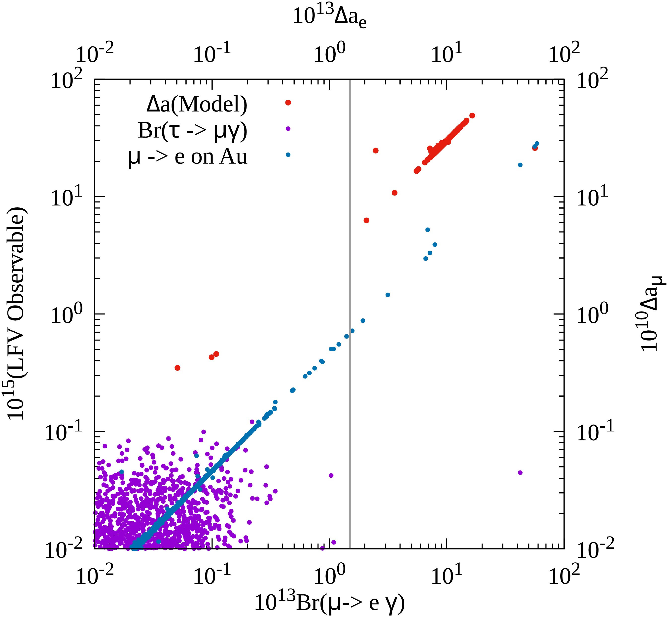
Figure 5. (color online) Low energy observables
$ \Delta a_{l} $ , Br$ \left(l_j \to l_i \gamma \right) $ and$ \mu \to e $ conversion rate on Au are presented for$ 10^4 $ randomly generated parameter points ($ 10^4 $ points for each observable). The points in red represent ($ \Delta a_{e}, \Delta a_{\mu} $ ), the ones in violet represent (Br$ \left(\mu \to e \gamma \right) $ , Br$ \left(\tau \to \mu \gamma \right) $ ) and the ones in blue show$ \mu \to e $ conversion rate on Au. The experimental limit on Br$ \left(\mu \to e \gamma \right) $ is shown by the dashed line. The experimental limits Br$ \left(\tau \to \mu \gamma \right) $ and$ \mu \to e $ conversion on Au are much weaker and hence, not shown.The values of Br
$ \left(\mu \to e \gamma \right) $ lie well below the upper bound of$ 1.5 \times 10^{-13} $ , as shown by the dashed line. The experimental limits for Br$ \left(\tau \to \mu \gamma \right) $ and$ \mu \to e $ conversion on Au are much weaker and hence, not shown. We observe the consistency of results with the electron and muon$ (g-2) $ anomalies as well as experimental bounds on the cLFV observables. In Tables 2 and 3, we list two sets of parameter points derived from this random scan. The two parameter space points represent two different mass hierarchies for the exotic particles, henceforth denoted as MH1 and MH2. The numerical values for low energy observables ($ \Delta a_{e}, \Delta a_{\mu} $ , and the cLFV branching ratios) pertaining to these two points are listed in Table 419 .Mass hierarchy 1 (MH1) Mass parameters/GeV Yukawa parameters $ \xi_{ z_{{RE}}}=1 $ ,$ \theta_{ z_{{RE}}}=35^0 $ ,$ \xi_{lE}=0.5 $ ,$ \eta_{lE}=1 $ ,$ \theta_{lE}=30^0 $ ,$ d_2=0.02 $ ,$ \theta_{R}=-55^0 $ $ \widetilde m_N=500 $ $ \widetilde m_E=600 $ $ \mu_{\Phi}=650 $ $ \widetilde m_L=850 $ $ z_{{RE}}:{\left(\begin{array}{*{20}{c}}{ 0.8192}&{0.5736}\\{-0.5736}&{0.8192 }\end{array}\right)} $ ,$ y_{{lE}}:{\left(\begin{array}{*{20}{c}}{ 0.4330}&{0.25}\\{-0.5}&{0.8660}\\{0}&{0 }\end{array}\right)} $ ,$ y_{{eL}}:{\left(\begin{array}{*{20}{c}}{ -0.06376}&{0.005577}\\{0.03757}&{0.4296}\\{0}&{0 }\end{array}\right)} $
$ y_{{lN}}:{\left(\begin{array}{*{20}{c}}{ 1.744\cdot 10^{-7}}&{4.072\cdot 10^{-6}}\\{-7.753\cdot 10^{-6}}&{8.995\cdot 10^{-6}}\\{-1.024\cdot 10^{-5}}&{1.86\cdot 10^{-6} }\end{array}\right)} \text{(NH)} $ ;$ {\left(\begin{array}{*{20}{c}}{ 3.002\cdot 10^{-7}}&{1.489\cdot 10^{-5}}\\{-9.674\cdot 10^{-6}}&{-1.426\cdot 10^{-6}}\\{1.158\cdot 10^{-5}}&{-1.714\cdot 10^{-6} }\end{array}\right)} \text{(IH)} $
$ z_{{LN}}:{\left(\begin{array}{*{20}{c}}{ 1.749\cdot 10^{-3}}&{-7.492\cdot 10^{-5}}\\{2\cdot 10^{-2}}&{-8.566\cdot 10^{-4} }\end{array}\right)} \text{(NH)} $ ;$ {\left(\begin{array}{*{20}{c}}{ 1.749\cdot 10^{-3}}&{-3.527\cdot 10^{-5}}\\{2\cdot 10^{-2}}&{-4.0320\cdot 10^{-4} }\end{array}\right)} \text{(IH)} $
Physical masses (GeV):$\{ \phi_P, \phi^\pm, \phi_S \} $ $ \sim $ $\{ 650,673,737 \} \quad $ $\{ {\widetilde N^S}, {\widetilde N^D_{a}}, {\widetilde N^D_{b}} \}$ $ \sim $ $\{ 500,850,850 \}\quad $ $\{ {\widetilde E^S}, {\widetilde E^D} \}$ $ \sim $ $\{ 511,939 \}$
Table 2. Input and output parameters for mass hierarchy, MH1, along with the physical mass spectrum that generates tiny neutrino masses and
$ \Delta a_\ell $ for the electron and muon, while also satisfying the experimental constraints on the lepton flavor violating (LFV) observables. The Yukawa couplings determined from the neutrino sector have been specified for the normal hierarchy (NH) and the inverted hierarchy (IH) of the neutrino mass spectrum. All the Yukawa parameters have been determined up to three decimal places to ensure$ z_{{RE}} \sim $ unitary,$ y_{{lE}} y_{{lE}}^{\dagger} \sim $ diagonal, and Br$ \left(\mu \to e \gamma \right) $ is within the constrained value.Mass hierarchy 2 (MH2) Mass parameters/GeV Yukawa parameters $ \xi_{ z_{{RE}}}=0.3 $ ,$ \theta_{ z_{{RE}}}=40^0 $ ,$ \xi_{lE}=0.9 $ ,$ \eta_{lE}=2 $ ,$ \theta_{lE}=75^0 $ ,$ d_2=0.017 $ ,$ \theta_{R}=-30^0 $ $ \widetilde m_N=470 $ $ \widetilde m_L=500 $ $ \widetilde m_E=1100 $ $ \mu_{\Phi}=1200 $ $ z_{{RE}}:{\left(\begin{array}{*{20}{c}}{0.2298}&{0.1928}\\{-0.1928}&{0.2298 }\end{array}\right)} $ ,$ y_{{lE}}:{\left(\begin{array}{*{20}{c}}{0.2329}&{0.8693}\\{-1.932}&{0.5176}\\{0}&{0 }\end{array}\right)} $ ,$ y_{{eL}}:{\left(\begin{array}{*{20}{c}}{-0.4532}&{-0.3174}\\{-1.940}&{2.770}\\{0}&{0 }\end{array}\right)} $
$ y_{{lN}}:{\left(\begin{array}{*{20}{c}}{2.927\cdot 10^{-6}}&{5.633\cdot 10^{-6}}\\{-5.024\cdot 10^{-6}}&{1.780\cdot 10^{-5}}\\{-1.324\cdot 10^{-5}}&{9.368\cdot 10^{-6} }\end{array}\right)} \text{(NH)} $ ;$ {\left(\begin{array}{*{20}{c}}{1.023\cdot 10^{-5}}&{2.082\cdot 10^{-5}}\\{-1.459\cdot 10^{-6}}&{4.356\cdot 10^{-5}}\\{1.522\cdot 10^{-5}}&{-1.004\cdot 10^{-5} }\end{array}\right)} \text{(IH)} $
$ z_{{LN}}:{\left(\begin{array}{*{20}{c}}{-1.191\cdot 10^{-2}}&{6.187\cdot 10^{-3}}\\{1.700\cdot 10^{-2}}&{-8.833\cdot 10^{-3} }\end{array}\right)} \text{(NH)} $ ;$ {\left(\begin{array}{*{20}{c}}{-1.191\cdot 10^{-2}}&{5.850\cdot 10^{-3}}\\{1.700\cdot 10^{-2}}&{-8.353\cdot 10^{-3} }\end{array}\right)} \text{(IH)} $
Physical masses (GeV):$\{ \phi_P, \phi^\pm, \phi_S \}$ $ \sim $ $\{ 1200, 1213, 1250 \} \quad $ ,$\{ {\widetilde N^S}, {\widetilde N^D_{a}}, {\widetilde N^D_{b}} \}$ $ \sim $ $\{ 470,500,500 \}\quad $ ,$\{ {\widetilde E^D}, {\widetilde E^S} \}$ $ \sim $ $\{ 496, 1105 \}$
Table 3. Same as Table 2, but for mass hierarchy MH2.
Low Energy Observable Expt. limit Model prediction for MH1 NH (IH) Model prediction for MH2 NH (IH) T $ - $ $ -4.19 \times 10^{-2} (-4.19 \times 10^{-2}) $ $ 0.787 \times 10^{-2} (0.787 \times 10^{-2}) $ S $ - $ $ -2.61 \times 10^{-2} (-2.61 \times 10^{-2}) $ $ -2.81 \times 10^{-3} (-2.81 \times 10^{-3}) $ U $ - $ $ -5.56 \times 10^{-4} (-5.56 \times 10^{-4}) $ $ -5.97 \times 10^{-4} (-5.97 \times 10^{-4}) $ ρ $ - $ $ -4.18 \times 10^{-5} (-4.18 \times 10^{-5}) $ $ -4.05 \times 10^{-4} (-4.05 \times 10^{-4}) $ $ 10^{12}\Delta a_{e} $ $ -0.88 \pm 0.36 $ [114]$ -1.07 (-1.07) $ $ -0.96 (-0.96) $ $ 10^{9}\Delta a_{\mu} $ $ 0.38\pm 0.64 $ [3, 115]$ 3.03 (3.03) $ $ 2.74 (2.74) $ Br $ \left(\mu^\pm \to e^\pm \gamma \right) $ $ 1.5 \times 10^{-13} $ [106]$ 7.09 \times 10^{-14} (7.09 \times 10^{-14}) $ $ 1.82 \times 10^{-14} (1.82 \times 10^{-14}) $ Br $ \left(\tau^\pm \to e^\pm \gamma \right) $ $ 3.3\times 10^{-8} $ [116]$ 1.12 \times 10^{-29} (1.74 \times 10^{-29}) $ $ 1.15 \times 10^{-25} (1.15 \times 10^{-25}) $ Br $ \left(\tau^\pm \to \mu^\pm \gamma \right) $ $ 4.4\times 10^{-8} $ [117]$ 1.46 \times 10^{-18} (1.86 \times 10^{-18}) $ $ 2.48 \times 10^{-16} (3.08 \times 10^{-16}) $ Br $ \left(\mu^+ \to e^+e^+e^- \right) $ $ 1.0\times 10^{-12} $ [107]$ 4.98 \times 10^{-16} (4.98 \times 10^{-16}) $ $ 1.29 \times 10^{-16} (1.29 \times 10^{-16}) $ Br $ \left(\tau^- \to e^-e^+e^- \right) $ $ 2.7\times 10^{-8} $ [118]$ 1.35 \times 10^{-31} (2.15 \times 10^{-31}) $ $ 1.38 \times 10^{-27} (1.39 \times 10^{-27}) $ Br $ \left(\tau^- \to \mu^-\mu^+\mu^- \right) $ $ 2.1\times 10^{-8} $ [118]$ 3.77 \times 10^{-21} (4.77 \times 10^{-21}) $ $ 6.39 \times 10^{-19} (7.92 \times 10^{-19}) $ Br $ \left(\tau^- \to e^-\mu^+\mu^- \right) $ $ 2.7\times 10^{-8} $ [118]$ 2.63 \times 10^{-32} (4.12 \times 10^{-32}) $ $ 2.72 \times 10^{-28} (3.00 \times 10^{-28}) $ Br $ \left(\tau^- \to \mu^-e^+e^- \right) $ $ 1.8\times 10^{-8} $ [118]$ 1.73 \times 10^{-20} (2.20 \times 10^{-20}) $ $ 2.94 \times 10^{-18} (3.64 \times 10^{-18}) $ Br $ \left(\tau^- \to e^+\mu^-\mu^- \right) $ $ 1.7\times 10^{-8} $ [118]$ 3.49 \times 10^{-43} (4.53 \times 10^{-43}) $ $ 4.43 \times 10^{-40} (5.75 \times 10^{-40}) $ Br $ \left(\tau^- \to \mu^+e^-e^- \right) $ $ 1.5\times 10^{-8} $ [118]$ 1.26 \times 10^{-45} (1.83 \times 10^{-44}) $ $ 1.60 \times 10^{-42} (2.31 \times 10^{-41}) $ $ \mu \to e $ on Pb$ 4.6\times 10^{-11} $ [119]$ 3.08 \times 10^{-16} (3.08 \times 10^{-16}) $ $ 7.96 \times 10^{-17} (7.95 \times 10^{-17}) $ $ \mu \to e $ on Ti$ 4.3\times 10^{-12} $ [120]$ 3.99 \times 10^{-16} (3.99 \times 10^{-16}) $ $ 1.04 \times 10^{-16} (1.04 \times 10^{-16}) $ $ \mu \to e $ on Au$ 7.0\times 10^{-13} $ [108]$ 3.28 \times 10^{-16} (3.28 \times 10^{-16}) $ $ 8.46 \times 10^{-17} (8.46 \times 10^{-17}) $ $ \mu \to e $ on Al$ 10^{-15} - 10^{-18} $ [109]$ 2.22 \times 10^{-16} (2.22 \times 10^{-16}) $ $ 5.79 \times 10^{-17} (5.79 \times 10^{-17}) $ -
For numerical evaluation of the
$ (g-2) $ and cLFV observables, we have implemented17 the model in${\mathrm{SARAH}}$ [110, 111], generated modules for${\mathrm{SPheno}}$ , and used${\mathrm{SPheno}}$ [112, 113] for the numerical evaluation. To validate our approach of constraining the parameter space of the model, we randomly generate$ 10^4 $ parameter points by varying the free parameters listed in Eq. (56). The mass parameters, namely,$ \widetilde m_N,\; \widetilde m_L,\; \widetilde m_E $ and$ \mu_{\Phi} $ , are varied in the range [400−1200] GeV. To avoid a charged particle as the lightest$ Z_2 $ -odd particle (L$ Z_2 $ OP), we ensure$ \widetilde m_N $ is always smaller than the other mass parameters. The Yukawa parameters in Eq. (56) are also randomly generated such that$ z_{{RE}}^{ij}\; \in\; [0.2-1.0],\; \; \; y_{{lE}}^{ij} \; \in\; [0.2-1.0],\; \; \; z_{{LN}}^{ij}\; \in\; [0.0-0.1]. $
(57) Note that
$ y_{{eL}} $ is inversely dependent on$ z_{{RE}} $ and$ y_{{lE}} $ in Eq. (42). The range of$ z_{{RE}}^{ij} $ and$ y_{{lE}}^{ij} $ in Eq. (57) is chosen to achieve$ y_{{eL}}^{ij}\sim{\cal O} \left(1 \right) $ or less. For$ z_{{LN}} $ (see Eq. (54) and the discussion following it), we select$ d_1=0 $ and vary$ d_2 $ so that$ z_{{LN}}^{ij} $ falls within the range specified in Eq. (57). The range of$ z_{{LN}}^{ij} $ is motivated to avoid constraints from dark matter direct detection experiments, which will be discussed in detail in the next section.For the
$ 10^4 $ parameter points generated, the numerical values of low energy observables$ \Delta a_{l} $ , Br$ \left(l_j \to l_i \gamma \right) $ , and the$ \mu \to e $ conversion rate on Au are presented for$ 10^4 $ randomly generated parameter points in Fig. 518 . The$ 10^4 $ points are plotted for three pairs of observables each, viz., in red for ($ \Delta a_{e}, \Delta a_{\mu} $ ), in violet for (Br$ \left(\mu \to e \gamma \right) $ , Br$ \left(\tau \to \mu \gamma \right) $ ), and in blue for (Br$ \left(\mu \to e \gamma \right) $ ,$ \mu \to e $ conversion on Au).
Figure 5. (color online) Low energy observables
$ \Delta a_{l} $ , Br$ \left(l_j \to l_i \gamma \right) $ and$ \mu \to e $ conversion rate on Au are presented for$ 10^4 $ randomly generated parameter points ($ 10^4 $ points for each observable). The points in red represent ($ \Delta a_{e}, \Delta a_{\mu} $ ), the ones in violet represent (Br$ \left(\mu \to e \gamma \right) $ , Br$ \left(\tau \to \mu \gamma \right) $ ) and the ones in blue show$ \mu \to e $ conversion rate on Au. The experimental limit on Br$ \left(\mu \to e \gamma \right) $ is shown by the dashed line. The experimental limits Br$ \left(\tau \to \mu \gamma \right) $ and$ \mu \to e $ conversion on Au are much weaker and hence, not shown.The values of Br
$ \left(\mu \to e \gamma \right) $ lie well below the upper bound of$ 1.5 \times 10^{-13} $ , as shown by the dashed line. The experimental limits for Br$ \left(\tau \to \mu \gamma \right) $ and$ \mu \to e $ conversion on Au are much weaker and hence, not shown. We observe the consistency of results with the electron and muon$ (g-2) $ anomalies as well as experimental bounds on the cLFV observables. In Tables 2 and 3, we list two sets of parameter points derived from this random scan. The two parameter space points represent two different mass hierarchies for the exotic particles, henceforth denoted as MH1 and MH2. The numerical values for low energy observables ($ \Delta a_{e}, \Delta a_{\mu} $ , and the cLFV branching ratios) pertaining to these two points are listed in Table 419 .Mass hierarchy 1 (MH1) Mass parameters/GeV Yukawa parameters $ \xi_{ z_{{RE}}}=1 $ ,$ \theta_{ z_{{RE}}}=35^0 $ ,$ \xi_{lE}=0.5 $ ,$ \eta_{lE}=1 $ ,$ \theta_{lE}=30^0 $ ,$ d_2=0.02 $ ,$ \theta_{R}=-55^0 $ $ \widetilde m_N=500 $ $ \widetilde m_E=600 $ $ \mu_{\Phi}=650 $ $ \widetilde m_L=850 $ $ z_{{RE}}:{\left(\begin{array}{*{20}{c}}{ 0.8192}&{0.5736}\\{-0.5736}&{0.8192 }\end{array}\right)} $ ,$ y_{{lE}}:{\left(\begin{array}{*{20}{c}}{ 0.4330}&{0.25}\\{-0.5}&{0.8660}\\{0}&{0 }\end{array}\right)} $ ,$ y_{{eL}}:{\left(\begin{array}{*{20}{c}}{ -0.06376}&{0.005577}\\{0.03757}&{0.4296}\\{0}&{0 }\end{array}\right)} $
$ y_{{lN}}:{\left(\begin{array}{*{20}{c}}{ 1.744\cdot 10^{-7}}&{4.072\cdot 10^{-6}}\\{-7.753\cdot 10^{-6}}&{8.995\cdot 10^{-6}}\\{-1.024\cdot 10^{-5}}&{1.86\cdot 10^{-6} }\end{array}\right)} \text{(NH)} $ ;$ {\left(\begin{array}{*{20}{c}}{ 3.002\cdot 10^{-7}}&{1.489\cdot 10^{-5}}\\{-9.674\cdot 10^{-6}}&{-1.426\cdot 10^{-6}}\\{1.158\cdot 10^{-5}}&{-1.714\cdot 10^{-6} }\end{array}\right)} \text{(IH)} $
$ z_{{LN}}:{\left(\begin{array}{*{20}{c}}{ 1.749\cdot 10^{-3}}&{-7.492\cdot 10^{-5}}\\{2\cdot 10^{-2}}&{-8.566\cdot 10^{-4} }\end{array}\right)} \text{(NH)} $ ;$ {\left(\begin{array}{*{20}{c}}{ 1.749\cdot 10^{-3}}&{-3.527\cdot 10^{-5}}\\{2\cdot 10^{-2}}&{-4.0320\cdot 10^{-4} }\end{array}\right)} \text{(IH)} $
Physical masses (GeV):$\{ \phi_P, \phi^\pm, \phi_S \} $ $ \sim $ $\{ 650,673,737 \} \quad $ $\{ {\widetilde N^S}, {\widetilde N^D_{a}}, {\widetilde N^D_{b}} \}$ $ \sim $ $\{ 500,850,850 \}\quad $ $\{ {\widetilde E^S}, {\widetilde E^D} \}$ $ \sim $ $\{ 511,939 \}$
Table 2. Input and output parameters for mass hierarchy, MH1, along with the physical mass spectrum that generates tiny neutrino masses and
$ \Delta a_\ell $ for the electron and muon, while also satisfying the experimental constraints on the lepton flavor violating (LFV) observables. The Yukawa couplings determined from the neutrino sector have been specified for the normal hierarchy (NH) and the inverted hierarchy (IH) of the neutrino mass spectrum. All the Yukawa parameters have been determined up to three decimal places to ensure$ z_{{RE}} \sim $ unitary,$ y_{{lE}} y_{{lE}}^{\dagger} \sim $ diagonal, and Br$ \left(\mu \to e \gamma \right) $ is within the constrained value.Mass hierarchy 2 (MH2) Mass parameters/GeV Yukawa parameters $ \xi_{ z_{{RE}}}=0.3 $ ,$ \theta_{ z_{{RE}}}=40^0 $ ,$ \xi_{lE}=0.9 $ ,$ \eta_{lE}=2 $ ,$ \theta_{lE}=75^0 $ ,$ d_2=0.017 $ ,$ \theta_{R}=-30^0 $ $ \widetilde m_N=470 $ $ \widetilde m_L=500 $ $ \widetilde m_E=1100 $ $ \mu_{\Phi}=1200 $ $ z_{{RE}}:{\left(\begin{array}{*{20}{c}}{0.2298}&{0.1928}\\{-0.1928}&{0.2298 }\end{array}\right)} $ ,$ y_{{lE}}:{\left(\begin{array}{*{20}{c}}{0.2329}&{0.8693}\\{-1.932}&{0.5176}\\{0}&{0 }\end{array}\right)} $ ,$ y_{{eL}}:{\left(\begin{array}{*{20}{c}}{-0.4532}&{-0.3174}\\{-1.940}&{2.770}\\{0}&{0 }\end{array}\right)} $
$ y_{{lN}}:{\left(\begin{array}{*{20}{c}}{2.927\cdot 10^{-6}}&{5.633\cdot 10^{-6}}\\{-5.024\cdot 10^{-6}}&{1.780\cdot 10^{-5}}\\{-1.324\cdot 10^{-5}}&{9.368\cdot 10^{-6} }\end{array}\right)} \text{(NH)} $ ;$ {\left(\begin{array}{*{20}{c}}{1.023\cdot 10^{-5}}&{2.082\cdot 10^{-5}}\\{-1.459\cdot 10^{-6}}&{4.356\cdot 10^{-5}}\\{1.522\cdot 10^{-5}}&{-1.004\cdot 10^{-5} }\end{array}\right)} \text{(IH)} $
$ z_{{LN}}:{\left(\begin{array}{*{20}{c}}{-1.191\cdot 10^{-2}}&{6.187\cdot 10^{-3}}\\{1.700\cdot 10^{-2}}&{-8.833\cdot 10^{-3} }\end{array}\right)} \text{(NH)} $ ;$ {\left(\begin{array}{*{20}{c}}{-1.191\cdot 10^{-2}}&{5.850\cdot 10^{-3}}\\{1.700\cdot 10^{-2}}&{-8.353\cdot 10^{-3} }\end{array}\right)} \text{(IH)} $
Physical masses (GeV):$\{ \phi_P, \phi^\pm, \phi_S \}$ $ \sim $ $\{ 1200, 1213, 1250 \} \quad $ ,$\{ {\widetilde N^S}, {\widetilde N^D_{a}}, {\widetilde N^D_{b}} \}$ $ \sim $ $\{ 470,500,500 \}\quad $ ,$\{ {\widetilde E^D}, {\widetilde E^S} \}$ $ \sim $ $\{ 496, 1105 \}$
Table 3. Same as Table 2, but for mass hierarchy MH2.
Low Energy Observable Expt. limit Model prediction for MH1 NH (IH) Model prediction for MH2 NH (IH) T $ - $ $ -4.19 \times 10^{-2} (-4.19 \times 10^{-2}) $ $ 0.787 \times 10^{-2} (0.787 \times 10^{-2}) $ S $ - $ $ -2.61 \times 10^{-2} (-2.61 \times 10^{-2}) $ $ -2.81 \times 10^{-3} (-2.81 \times 10^{-3}) $ U $ - $ $ -5.56 \times 10^{-4} (-5.56 \times 10^{-4}) $ $ -5.97 \times 10^{-4} (-5.97 \times 10^{-4}) $ ρ $ - $ $ -4.18 \times 10^{-5} (-4.18 \times 10^{-5}) $ $ -4.05 \times 10^{-4} (-4.05 \times 10^{-4}) $ $ 10^{12}\Delta a_{e} $ $ -0.88 \pm 0.36 $ [114]$ -1.07 (-1.07) $ $ -0.96 (-0.96) $ $ 10^{9}\Delta a_{\mu} $ $ 0.38\pm 0.64 $ [3, 115]$ 3.03 (3.03) $ $ 2.74 (2.74) $ Br $ \left(\mu^\pm \to e^\pm \gamma \right) $ $ 1.5 \times 10^{-13} $ [106]$ 7.09 \times 10^{-14} (7.09 \times 10^{-14}) $ $ 1.82 \times 10^{-14} (1.82 \times 10^{-14}) $ Br $ \left(\tau^\pm \to e^\pm \gamma \right) $ $ 3.3\times 10^{-8} $ [116]$ 1.12 \times 10^{-29} (1.74 \times 10^{-29}) $ $ 1.15 \times 10^{-25} (1.15 \times 10^{-25}) $ Br $ \left(\tau^\pm \to \mu^\pm \gamma \right) $ $ 4.4\times 10^{-8} $ [117]$ 1.46 \times 10^{-18} (1.86 \times 10^{-18}) $ $ 2.48 \times 10^{-16} (3.08 \times 10^{-16}) $ Br $ \left(\mu^+ \to e^+e^+e^- \right) $ $ 1.0\times 10^{-12} $ [107]$ 4.98 \times 10^{-16} (4.98 \times 10^{-16}) $ $ 1.29 \times 10^{-16} (1.29 \times 10^{-16}) $ Br $ \left(\tau^- \to e^-e^+e^- \right) $ $ 2.7\times 10^{-8} $ [118]$ 1.35 \times 10^{-31} (2.15 \times 10^{-31}) $ $ 1.38 \times 10^{-27} (1.39 \times 10^{-27}) $ Br $ \left(\tau^- \to \mu^-\mu^+\mu^- \right) $ $ 2.1\times 10^{-8} $ [118]$ 3.77 \times 10^{-21} (4.77 \times 10^{-21}) $ $ 6.39 \times 10^{-19} (7.92 \times 10^{-19}) $ Br $ \left(\tau^- \to e^-\mu^+\mu^- \right) $ $ 2.7\times 10^{-8} $ [118]$ 2.63 \times 10^{-32} (4.12 \times 10^{-32}) $ $ 2.72 \times 10^{-28} (3.00 \times 10^{-28}) $ Br $ \left(\tau^- \to \mu^-e^+e^- \right) $ $ 1.8\times 10^{-8} $ [118]$ 1.73 \times 10^{-20} (2.20 \times 10^{-20}) $ $ 2.94 \times 10^{-18} (3.64 \times 10^{-18}) $ Br $ \left(\tau^- \to e^+\mu^-\mu^- \right) $ $ 1.7\times 10^{-8} $ [118]$ 3.49 \times 10^{-43} (4.53 \times 10^{-43}) $ $ 4.43 \times 10^{-40} (5.75 \times 10^{-40}) $ Br $ \left(\tau^- \to \mu^+e^-e^- \right) $ $ 1.5\times 10^{-8} $ [118]$ 1.26 \times 10^{-45} (1.83 \times 10^{-44}) $ $ 1.60 \times 10^{-42} (2.31 \times 10^{-41}) $ $ \mu \to e $ on Pb$ 4.6\times 10^{-11} $ [119]$ 3.08 \times 10^{-16} (3.08 \times 10^{-16}) $ $ 7.96 \times 10^{-17} (7.95 \times 10^{-17}) $ $ \mu \to e $ on Ti$ 4.3\times 10^{-12} $ [120]$ 3.99 \times 10^{-16} (3.99 \times 10^{-16}) $ $ 1.04 \times 10^{-16} (1.04 \times 10^{-16}) $ $ \mu \to e $ on Au$ 7.0\times 10^{-13} $ [108]$ 3.28 \times 10^{-16} (3.28 \times 10^{-16}) $ $ 8.46 \times 10^{-17} (8.46 \times 10^{-17}) $ $ \mu \to e $ on Al$ 10^{-15} - 10^{-18} $ [109]$ 2.22 \times 10^{-16} (2.22 \times 10^{-16}) $ $ 5.79 \times 10^{-17} (5.79 \times 10^{-17}) $ -
For numerical evaluation of the
$ (g-2) $ and cLFV observables, we have implemented17 the model in${\mathrm{SARAH}}$ [110, 111], generated modules for${\mathrm{SPheno}}$ , and used${\mathrm{SPheno}}$ [112, 113] for the numerical evaluation. To validate our approach of constraining the parameter space of the model, we randomly generate$ 10^4 $ parameter points by varying the free parameters listed in Eq. (56). The mass parameters, namely,$ \widetilde m_N,\; \widetilde m_L,\; \widetilde m_E $ and$ \mu_{\Phi} $ , are varied in the range [400−1200] GeV. To avoid a charged particle as the lightest$ Z_2 $ -odd particle (L$ Z_2 $ OP), we ensure$ \widetilde m_N $ is always smaller than the other mass parameters. The Yukawa parameters in Eq. (56) are also randomly generated such that$ z_{{RE}}^{ij}\; \in\; [0.2-1.0],\; \; \; y_{{lE}}^{ij} \; \in\; [0.2-1.0],\; \; \; z_{{LN}}^{ij}\; \in\; [0.0-0.1]. $
(57) Note that
$ y_{{eL}} $ is inversely dependent on$ z_{{RE}} $ and$ y_{{lE}} $ in Eq. (42). The range of$ z_{{RE}}^{ij} $ and$ y_{{lE}}^{ij} $ in Eq. (57) is chosen to achieve$ y_{{eL}}^{ij}\sim{\cal O} \left(1 \right) $ or less. For$ z_{{LN}} $ (see Eq. (54) and the discussion following it), we select$ d_1=0 $ and vary$ d_2 $ so that$ z_{{LN}}^{ij} $ falls within the range specified in Eq. (57). The range of$ z_{{LN}}^{ij} $ is motivated to avoid constraints from dark matter direct detection experiments, which will be discussed in detail in the next section.For the
$ 10^4 $ parameter points generated, the numerical values of low energy observables$ \Delta a_{l} $ , Br$ \left(l_j \to l_i \gamma \right) $ , and the$ \mu \to e $ conversion rate on Au are presented for$ 10^4 $ randomly generated parameter points in Fig. 518 . The$ 10^4 $ points are plotted for three pairs of observables each, viz., in red for ($ \Delta a_{e}, \Delta a_{\mu} $ ), in violet for (Br$ \left(\mu \to e \gamma \right) $ , Br$ \left(\tau \to \mu \gamma \right) $ ), and in blue for (Br$ \left(\mu \to e \gamma \right) $ ,$ \mu \to e $ conversion on Au).
Figure 5. (color online) Low energy observables
$ \Delta a_{l} $ , Br$ \left(l_j \to l_i \gamma \right) $ and$ \mu \to e $ conversion rate on Au are presented for$ 10^4 $ randomly generated parameter points ($ 10^4 $ points for each observable). The points in red represent ($ \Delta a_{e}, \Delta a_{\mu} $ ), the ones in violet represent (Br$ \left(\mu \to e \gamma \right) $ , Br$ \left(\tau \to \mu \gamma \right) $ ) and the ones in blue show$ \mu \to e $ conversion rate on Au. The experimental limit on Br$ \left(\mu \to e \gamma \right) $ is shown by the dashed line. The experimental limits Br$ \left(\tau \to \mu \gamma \right) $ and$ \mu \to e $ conversion on Au are much weaker and hence, not shown.The values of Br
$ \left(\mu \to e \gamma \right) $ lie well below the upper bound of$ 1.5 \times 10^{-13} $ , as shown by the dashed line. The experimental limits for Br$ \left(\tau \to \mu \gamma \right) $ and$ \mu \to e $ conversion on Au are much weaker and hence, not shown. We observe the consistency of results with the electron and muon$ (g-2) $ anomalies as well as experimental bounds on the cLFV observables. In Tables 2 and 3, we list two sets of parameter points derived from this random scan. The two parameter space points represent two different mass hierarchies for the exotic particles, henceforth denoted as MH1 and MH2. The numerical values for low energy observables ($ \Delta a_{e}, \Delta a_{\mu} $ , and the cLFV branching ratios) pertaining to these two points are listed in Table 419 .Mass hierarchy 1 (MH1) Mass parameters/GeV Yukawa parameters $ \xi_{ z_{{RE}}}=1 $ ,$ \theta_{ z_{{RE}}}=35^0 $ ,$ \xi_{lE}=0.5 $ ,$ \eta_{lE}=1 $ ,$ \theta_{lE}=30^0 $ ,$ d_2=0.02 $ ,$ \theta_{R}=-55^0 $ $ \widetilde m_N=500 $ $ \widetilde m_E=600 $ $ \mu_{\Phi}=650 $ $ \widetilde m_L=850 $ $ z_{{RE}}:{\left(\begin{array}{*{20}{c}}{ 0.8192}&{0.5736}\\{-0.5736}&{0.8192 }\end{array}\right)} $ ,$ y_{{lE}}:{\left(\begin{array}{*{20}{c}}{ 0.4330}&{0.25}\\{-0.5}&{0.8660}\\{0}&{0 }\end{array}\right)} $ ,$ y_{{eL}}:{\left(\begin{array}{*{20}{c}}{ -0.06376}&{0.005577}\\{0.03757}&{0.4296}\\{0}&{0 }\end{array}\right)} $
$ y_{{lN}}:{\left(\begin{array}{*{20}{c}}{ 1.744\cdot 10^{-7}}&{4.072\cdot 10^{-6}}\\{-7.753\cdot 10^{-6}}&{8.995\cdot 10^{-6}}\\{-1.024\cdot 10^{-5}}&{1.86\cdot 10^{-6} }\end{array}\right)} \text{(NH)} $ ;$ {\left(\begin{array}{*{20}{c}}{ 3.002\cdot 10^{-7}}&{1.489\cdot 10^{-5}}\\{-9.674\cdot 10^{-6}}&{-1.426\cdot 10^{-6}}\\{1.158\cdot 10^{-5}}&{-1.714\cdot 10^{-6} }\end{array}\right)} \text{(IH)} $
$ z_{{LN}}:{\left(\begin{array}{*{20}{c}}{ 1.749\cdot 10^{-3}}&{-7.492\cdot 10^{-5}}\\{2\cdot 10^{-2}}&{-8.566\cdot 10^{-4} }\end{array}\right)} \text{(NH)} $ ;$ {\left(\begin{array}{*{20}{c}}{ 1.749\cdot 10^{-3}}&{-3.527\cdot 10^{-5}}\\{2\cdot 10^{-2}}&{-4.0320\cdot 10^{-4} }\end{array}\right)} \text{(IH)} $
Physical masses (GeV):$\{ \phi_P, \phi^\pm, \phi_S \} $ $ \sim $ $\{ 650,673,737 \} \quad $ $\{ {\widetilde N^S}, {\widetilde N^D_{a}}, {\widetilde N^D_{b}} \}$ $ \sim $ $\{ 500,850,850 \}\quad $ $\{ {\widetilde E^S}, {\widetilde E^D} \}$ $ \sim $ $\{ 511,939 \}$
Table 2. Input and output parameters for mass hierarchy, MH1, along with the physical mass spectrum that generates tiny neutrino masses and
$ \Delta a_\ell $ for the electron and muon, while also satisfying the experimental constraints on the lepton flavor violating (LFV) observables. The Yukawa couplings determined from the neutrino sector have been specified for the normal hierarchy (NH) and the inverted hierarchy (IH) of the neutrino mass spectrum. All the Yukawa parameters have been determined up to three decimal places to ensure$ z_{{RE}} \sim $ unitary,$ y_{{lE}} y_{{lE}}^{\dagger} \sim $ diagonal, and Br$ \left(\mu \to e \gamma \right) $ is within the constrained value.Mass hierarchy 2 (MH2) Mass parameters/GeV Yukawa parameters $ \xi_{ z_{{RE}}}=0.3 $ ,$ \theta_{ z_{{RE}}}=40^0 $ ,$ \xi_{lE}=0.9 $ ,$ \eta_{lE}=2 $ ,$ \theta_{lE}=75^0 $ ,$ d_2=0.017 $ ,$ \theta_{R}=-30^0 $ $ \widetilde m_N=470 $ $ \widetilde m_L=500 $ $ \widetilde m_E=1100 $ $ \mu_{\Phi}=1200 $ $ z_{{RE}}:{\left(\begin{array}{*{20}{c}}{0.2298}&{0.1928}\\{-0.1928}&{0.2298 }\end{array}\right)} $ ,$ y_{{lE}}:{\left(\begin{array}{*{20}{c}}{0.2329}&{0.8693}\\{-1.932}&{0.5176}\\{0}&{0 }\end{array}\right)} $ ,$ y_{{eL}}:{\left(\begin{array}{*{20}{c}}{-0.4532}&{-0.3174}\\{-1.940}&{2.770}\\{0}&{0 }\end{array}\right)} $
$ y_{{lN}}:{\left(\begin{array}{*{20}{c}}{2.927\cdot 10^{-6}}&{5.633\cdot 10^{-6}}\\{-5.024\cdot 10^{-6}}&{1.780\cdot 10^{-5}}\\{-1.324\cdot 10^{-5}}&{9.368\cdot 10^{-6} }\end{array}\right)} \text{(NH)} $ ;$ {\left(\begin{array}{*{20}{c}}{1.023\cdot 10^{-5}}&{2.082\cdot 10^{-5}}\\{-1.459\cdot 10^{-6}}&{4.356\cdot 10^{-5}}\\{1.522\cdot 10^{-5}}&{-1.004\cdot 10^{-5} }\end{array}\right)} \text{(IH)} $
$ z_{{LN}}:{\left(\begin{array}{*{20}{c}}{-1.191\cdot 10^{-2}}&{6.187\cdot 10^{-3}}\\{1.700\cdot 10^{-2}}&{-8.833\cdot 10^{-3} }\end{array}\right)} \text{(NH)} $ ;$ {\left(\begin{array}{*{20}{c}}{-1.191\cdot 10^{-2}}&{5.850\cdot 10^{-3}}\\{1.700\cdot 10^{-2}}&{-8.353\cdot 10^{-3} }\end{array}\right)} \text{(IH)} $
Physical masses (GeV):$\{ \phi_P, \phi^\pm, \phi_S \}$ $ \sim $ $\{ 1200, 1213, 1250 \} \quad $ ,$\{ {\widetilde N^S}, {\widetilde N^D_{a}}, {\widetilde N^D_{b}} \}$ $ \sim $ $\{ 470,500,500 \}\quad $ ,$\{ {\widetilde E^D}, {\widetilde E^S} \}$ $ \sim $ $\{ 496, 1105 \}$
Table 3. Same as Table 2, but for mass hierarchy MH2.
Low Energy Observable Expt. limit Model prediction for MH1 NH (IH) Model prediction for MH2 NH (IH) T $ - $ $ -4.19 \times 10^{-2} (-4.19 \times 10^{-2}) $ $ 0.787 \times 10^{-2} (0.787 \times 10^{-2}) $ S $ - $ $ -2.61 \times 10^{-2} (-2.61 \times 10^{-2}) $ $ -2.81 \times 10^{-3} (-2.81 \times 10^{-3}) $ U $ - $ $ -5.56 \times 10^{-4} (-5.56 \times 10^{-4}) $ $ -5.97 \times 10^{-4} (-5.97 \times 10^{-4}) $ ρ $ - $ $ -4.18 \times 10^{-5} (-4.18 \times 10^{-5}) $ $ -4.05 \times 10^{-4} (-4.05 \times 10^{-4}) $ $ 10^{12}\Delta a_{e} $ $ -0.88 \pm 0.36 $ [114]$ -1.07 (-1.07) $ $ -0.96 (-0.96) $ $ 10^{9}\Delta a_{\mu} $ $ 0.38\pm 0.64 $ [3, 115]$ 3.03 (3.03) $ $ 2.74 (2.74) $ Br $ \left(\mu^\pm \to e^\pm \gamma \right) $ $ 1.5 \times 10^{-13} $ [106]$ 7.09 \times 10^{-14} (7.09 \times 10^{-14}) $ $ 1.82 \times 10^{-14} (1.82 \times 10^{-14}) $ Br $ \left(\tau^\pm \to e^\pm \gamma \right) $ $ 3.3\times 10^{-8} $ [116]$ 1.12 \times 10^{-29} (1.74 \times 10^{-29}) $ $ 1.15 \times 10^{-25} (1.15 \times 10^{-25}) $ Br $ \left(\tau^\pm \to \mu^\pm \gamma \right) $ $ 4.4\times 10^{-8} $ [117]$ 1.46 \times 10^{-18} (1.86 \times 10^{-18}) $ $ 2.48 \times 10^{-16} (3.08 \times 10^{-16}) $ Br $ \left(\mu^+ \to e^+e^+e^- \right) $ $ 1.0\times 10^{-12} $ [107]$ 4.98 \times 10^{-16} (4.98 \times 10^{-16}) $ $ 1.29 \times 10^{-16} (1.29 \times 10^{-16}) $ Br $ \left(\tau^- \to e^-e^+e^- \right) $ $ 2.7\times 10^{-8} $ [118]$ 1.35 \times 10^{-31} (2.15 \times 10^{-31}) $ $ 1.38 \times 10^{-27} (1.39 \times 10^{-27}) $ Br $ \left(\tau^- \to \mu^-\mu^+\mu^- \right) $ $ 2.1\times 10^{-8} $ [118]$ 3.77 \times 10^{-21} (4.77 \times 10^{-21}) $ $ 6.39 \times 10^{-19} (7.92 \times 10^{-19}) $ Br $ \left(\tau^- \to e^-\mu^+\mu^- \right) $ $ 2.7\times 10^{-8} $ [118]$ 2.63 \times 10^{-32} (4.12 \times 10^{-32}) $ $ 2.72 \times 10^{-28} (3.00 \times 10^{-28}) $ Br $ \left(\tau^- \to \mu^-e^+e^- \right) $ $ 1.8\times 10^{-8} $ [118]$ 1.73 \times 10^{-20} (2.20 \times 10^{-20}) $ $ 2.94 \times 10^{-18} (3.64 \times 10^{-18}) $ Br $ \left(\tau^- \to e^+\mu^-\mu^- \right) $ $ 1.7\times 10^{-8} $ [118]$ 3.49 \times 10^{-43} (4.53 \times 10^{-43}) $ $ 4.43 \times 10^{-40} (5.75 \times 10^{-40}) $ Br $ \left(\tau^- \to \mu^+e^-e^- \right) $ $ 1.5\times 10^{-8} $ [118]$ 1.26 \times 10^{-45} (1.83 \times 10^{-44}) $ $ 1.60 \times 10^{-42} (2.31 \times 10^{-41}) $ $ \mu \to e $ on Pb$ 4.6\times 10^{-11} $ [119]$ 3.08 \times 10^{-16} (3.08 \times 10^{-16}) $ $ 7.96 \times 10^{-17} (7.95 \times 10^{-17}) $ $ \mu \to e $ on Ti$ 4.3\times 10^{-12} $ [120]$ 3.99 \times 10^{-16} (3.99 \times 10^{-16}) $ $ 1.04 \times 10^{-16} (1.04 \times 10^{-16}) $ $ \mu \to e $ on Au$ 7.0\times 10^{-13} $ [108]$ 3.28 \times 10^{-16} (3.28 \times 10^{-16}) $ $ 8.46 \times 10^{-17} (8.46 \times 10^{-17}) $ $ \mu \to e $ on Al$ 10^{-15} - 10^{-18} $ [109]$ 2.22 \times 10^{-16} (2.22 \times 10^{-16}) $ $ 5.79 \times 10^{-17} (5.79 \times 10^{-17}) $ -
For numerical evaluation of the
$ (g-2) $ and cLFV observables, we have implemented17 the model in${\mathrm{SARAH}}$ [110, 111], generated modules for${\mathrm{SPheno}}$ , and used${\mathrm{SPheno}}$ [112, 113] for the numerical evaluation. To validate our approach of constraining the parameter space of the model, we randomly generate$ 10^4 $ parameter points by varying the free parameters listed in Eq. (56). The mass parameters, namely,$ \widetilde m_N,\; \widetilde m_L,\; \widetilde m_E $ and$ \mu_{\Phi} $ , are varied in the range [400−1200] GeV. To avoid a charged particle as the lightest$ Z_2 $ -odd particle (L$ Z_2 $ OP), we ensure$ \widetilde m_N $ is always smaller than the other mass parameters. The Yukawa parameters in Eq. (56) are also randomly generated such that$ z_{{RE}}^{ij}\; \in\; [0.2-1.0],\; \; \; y_{{lE}}^{ij} \; \in\; [0.2-1.0],\; \; \; z_{{LN}}^{ij}\; \in\; [0.0-0.1]. $
(57) Note that
$ y_{{eL}} $ is inversely dependent on$ z_{{RE}} $ and$ y_{{lE}} $ in Eq. (42). The range of$ z_{{RE}}^{ij} $ and$ y_{{lE}}^{ij} $ in Eq. (57) is chosen to achieve$ y_{{eL}}^{ij}\sim{\cal O} \left(1 \right) $ or less. For$ z_{{LN}} $ (see Eq. (54) and the discussion following it), we select$ d_1=0 $ and vary$ d_2 $ so that$ z_{{LN}}^{ij} $ falls within the range specified in Eq. (57). The range of$ z_{{LN}}^{ij} $ is motivated to avoid constraints from dark matter direct detection experiments, which will be discussed in detail in the next section.For the
$ 10^4 $ parameter points generated, the numerical values of low energy observables$ \Delta a_{l} $ , Br$ \left(l_j \to l_i \gamma \right) $ , and the$ \mu \to e $ conversion rate on Au are presented for$ 10^4 $ randomly generated parameter points in Fig. 518 . The$ 10^4 $ points are plotted for three pairs of observables each, viz., in red for ($ \Delta a_{e}, \Delta a_{\mu} $ ), in violet for (Br$ \left(\mu \to e \gamma \right) $ , Br$ \left(\tau \to \mu \gamma \right) $ ), and in blue for (Br$ \left(\mu \to e \gamma \right) $ ,$ \mu \to e $ conversion on Au).
Figure 5. (color online) Low energy observables
$ \Delta a_{l} $ , Br$ \left(l_j \to l_i \gamma \right) $ and$ \mu \to e $ conversion rate on Au are presented for$ 10^4 $ randomly generated parameter points ($ 10^4 $ points for each observable). The points in red represent ($ \Delta a_{e}, \Delta a_{\mu} $ ), the ones in violet represent (Br$ \left(\mu \to e \gamma \right) $ , Br$ \left(\tau \to \mu \gamma \right) $ ) and the ones in blue show$ \mu \to e $ conversion rate on Au. The experimental limit on Br$ \left(\mu \to e \gamma \right) $ is shown by the dashed line. The experimental limits Br$ \left(\tau \to \mu \gamma \right) $ and$ \mu \to e $ conversion on Au are much weaker and hence, not shown.The values of Br
$ \left(\mu \to e \gamma \right) $ lie well below the upper bound of$ 1.5 \times 10^{-13} $ , as shown by the dashed line. The experimental limits for Br$ \left(\tau \to \mu \gamma \right) $ and$ \mu \to e $ conversion on Au are much weaker and hence, not shown. We observe the consistency of results with the electron and muon$ (g-2) $ anomalies as well as experimental bounds on the cLFV observables. In Tables 2 and 3, we list two sets of parameter points derived from this random scan. The two parameter space points represent two different mass hierarchies for the exotic particles, henceforth denoted as MH1 and MH2. The numerical values for low energy observables ($ \Delta a_{e}, \Delta a_{\mu} $ , and the cLFV branching ratios) pertaining to these two points are listed in Table 419 .Mass hierarchy 1 (MH1) Mass parameters/GeV Yukawa parameters $ \xi_{ z_{{RE}}}=1 $ ,$ \theta_{ z_{{RE}}}=35^0 $ ,$ \xi_{lE}=0.5 $ ,$ \eta_{lE}=1 $ ,$ \theta_{lE}=30^0 $ ,$ d_2=0.02 $ ,$ \theta_{R}=-55^0 $ $ \widetilde m_N=500 $ $ \widetilde m_E=600 $ $ \mu_{\Phi}=650 $ $ \widetilde m_L=850 $ $ z_{{RE}}:{\left(\begin{array}{*{20}{c}}{ 0.8192}&{0.5736}\\{-0.5736}&{0.8192 }\end{array}\right)} $ ,$ y_{{lE}}:{\left(\begin{array}{*{20}{c}}{ 0.4330}&{0.25}\\{-0.5}&{0.8660}\\{0}&{0 }\end{array}\right)} $ ,$ y_{{eL}}:{\left(\begin{array}{*{20}{c}}{ -0.06376}&{0.005577}\\{0.03757}&{0.4296}\\{0}&{0 }\end{array}\right)} $
$ y_{{lN}}:{\left(\begin{array}{*{20}{c}}{ 1.744\cdot 10^{-7}}&{4.072\cdot 10^{-6}}\\{-7.753\cdot 10^{-6}}&{8.995\cdot 10^{-6}}\\{-1.024\cdot 10^{-5}}&{1.86\cdot 10^{-6} }\end{array}\right)} \text{(NH)} $ ;$ {\left(\begin{array}{*{20}{c}}{ 3.002\cdot 10^{-7}}&{1.489\cdot 10^{-5}}\\{-9.674\cdot 10^{-6}}&{-1.426\cdot 10^{-6}}\\{1.158\cdot 10^{-5}}&{-1.714\cdot 10^{-6} }\end{array}\right)} \text{(IH)} $
$ z_{{LN}}:{\left(\begin{array}{*{20}{c}}{ 1.749\cdot 10^{-3}}&{-7.492\cdot 10^{-5}}\\{2\cdot 10^{-2}}&{-8.566\cdot 10^{-4} }\end{array}\right)} \text{(NH)} $ ;$ {\left(\begin{array}{*{20}{c}}{ 1.749\cdot 10^{-3}}&{-3.527\cdot 10^{-5}}\\{2\cdot 10^{-2}}&{-4.0320\cdot 10^{-4} }\end{array}\right)} \text{(IH)} $
Physical masses (GeV):$\{ \phi_P, \phi^\pm, \phi_S \} $ $ \sim $ $\{ 650,673,737 \} \quad $ $\{ {\widetilde N^S}, {\widetilde N^D_{a}}, {\widetilde N^D_{b}} \}$ $ \sim $ $\{ 500,850,850 \}\quad $ $\{ {\widetilde E^S}, {\widetilde E^D} \}$ $ \sim $ $\{ 511,939 \}$
Table 2. Input and output parameters for mass hierarchy, MH1, along with the physical mass spectrum that generates tiny neutrino masses and
$ \Delta a_\ell $ for the electron and muon, while also satisfying the experimental constraints on the lepton flavor violating (LFV) observables. The Yukawa couplings determined from the neutrino sector have been specified for the normal hierarchy (NH) and the inverted hierarchy (IH) of the neutrino mass spectrum. All the Yukawa parameters have been determined up to three decimal places to ensure$ z_{{RE}} \sim $ unitary,$ y_{{lE}} y_{{lE}}^{\dagger} \sim $ diagonal, and Br$ \left(\mu \to e \gamma \right) $ is within the constrained value.Mass hierarchy 2 (MH2) Mass parameters/GeV Yukawa parameters $ \xi_{ z_{{RE}}}=0.3 $ ,$ \theta_{ z_{{RE}}}=40^0 $ ,$ \xi_{lE}=0.9 $ ,$ \eta_{lE}=2 $ ,$ \theta_{lE}=75^0 $ ,$ d_2=0.017 $ ,$ \theta_{R}=-30^0 $ $ \widetilde m_N=470 $ $ \widetilde m_L=500 $ $ \widetilde m_E=1100 $ $ \mu_{\Phi}=1200 $ $ z_{{RE}}:{\left(\begin{array}{*{20}{c}}{0.2298}&{0.1928}\\{-0.1928}&{0.2298 }\end{array}\right)} $ ,$ y_{{lE}}:{\left(\begin{array}{*{20}{c}}{0.2329}&{0.8693}\\{-1.932}&{0.5176}\\{0}&{0 }\end{array}\right)} $ ,$ y_{{eL}}:{\left(\begin{array}{*{20}{c}}{-0.4532}&{-0.3174}\\{-1.940}&{2.770}\\{0}&{0 }\end{array}\right)} $
$ y_{{lN}}:{\left(\begin{array}{*{20}{c}}{2.927\cdot 10^{-6}}&{5.633\cdot 10^{-6}}\\{-5.024\cdot 10^{-6}}&{1.780\cdot 10^{-5}}\\{-1.324\cdot 10^{-5}}&{9.368\cdot 10^{-6} }\end{array}\right)} \text{(NH)} $ ;$ {\left(\begin{array}{*{20}{c}}{1.023\cdot 10^{-5}}&{2.082\cdot 10^{-5}}\\{-1.459\cdot 10^{-6}}&{4.356\cdot 10^{-5}}\\{1.522\cdot 10^{-5}}&{-1.004\cdot 10^{-5} }\end{array}\right)} \text{(IH)} $
$ z_{{LN}}:{\left(\begin{array}{*{20}{c}}{-1.191\cdot 10^{-2}}&{6.187\cdot 10^{-3}}\\{1.700\cdot 10^{-2}}&{-8.833\cdot 10^{-3} }\end{array}\right)} \text{(NH)} $ ;$ {\left(\begin{array}{*{20}{c}}{-1.191\cdot 10^{-2}}&{5.850\cdot 10^{-3}}\\{1.700\cdot 10^{-2}}&{-8.353\cdot 10^{-3} }\end{array}\right)} \text{(IH)} $
Physical masses (GeV):$\{ \phi_P, \phi^\pm, \phi_S \}$ $ \sim $ $\{ 1200, 1213, 1250 \} \quad $ ,$\{ {\widetilde N^S}, {\widetilde N^D_{a}}, {\widetilde N^D_{b}} \}$ $ \sim $ $\{ 470,500,500 \}\quad $ ,$\{ {\widetilde E^D}, {\widetilde E^S} \}$ $ \sim $ $\{ 496, 1105 \}$
Table 3. Same as Table 2, but for mass hierarchy MH2.
Low Energy Observable Expt. limit Model prediction for MH1 NH (IH) Model prediction for MH2 NH (IH) T $ - $ $ -4.19 \times 10^{-2} (-4.19 \times 10^{-2}) $ $ 0.787 \times 10^{-2} (0.787 \times 10^{-2}) $ S $ - $ $ -2.61 \times 10^{-2} (-2.61 \times 10^{-2}) $ $ -2.81 \times 10^{-3} (-2.81 \times 10^{-3}) $ U $ - $ $ -5.56 \times 10^{-4} (-5.56 \times 10^{-4}) $ $ -5.97 \times 10^{-4} (-5.97 \times 10^{-4}) $ ρ $ - $ $ -4.18 \times 10^{-5} (-4.18 \times 10^{-5}) $ $ -4.05 \times 10^{-4} (-4.05 \times 10^{-4}) $ $ 10^{12}\Delta a_{e} $ $ -0.88 \pm 0.36 $ [114]$ -1.07 (-1.07) $ $ -0.96 (-0.96) $ $ 10^{9}\Delta a_{\mu} $ $ 0.38\pm 0.64 $ [3, 115]$ 3.03 (3.03) $ $ 2.74 (2.74) $ Br $ \left(\mu^\pm \to e^\pm \gamma \right) $ $ 1.5 \times 10^{-13} $ [106]$ 7.09 \times 10^{-14} (7.09 \times 10^{-14}) $ $ 1.82 \times 10^{-14} (1.82 \times 10^{-14}) $ Br $ \left(\tau^\pm \to e^\pm \gamma \right) $ $ 3.3\times 10^{-8} $ [116]$ 1.12 \times 10^{-29} (1.74 \times 10^{-29}) $ $ 1.15 \times 10^{-25} (1.15 \times 10^{-25}) $ Br $ \left(\tau^\pm \to \mu^\pm \gamma \right) $ $ 4.4\times 10^{-8} $ [117]$ 1.46 \times 10^{-18} (1.86 \times 10^{-18}) $ $ 2.48 \times 10^{-16} (3.08 \times 10^{-16}) $ Br $ \left(\mu^+ \to e^+e^+e^- \right) $ $ 1.0\times 10^{-12} $ [107]$ 4.98 \times 10^{-16} (4.98 \times 10^{-16}) $ $ 1.29 \times 10^{-16} (1.29 \times 10^{-16}) $ Br $ \left(\tau^- \to e^-e^+e^- \right) $ $ 2.7\times 10^{-8} $ [118]$ 1.35 \times 10^{-31} (2.15 \times 10^{-31}) $ $ 1.38 \times 10^{-27} (1.39 \times 10^{-27}) $ Br $ \left(\tau^- \to \mu^-\mu^+\mu^- \right) $ $ 2.1\times 10^{-8} $ [118]$ 3.77 \times 10^{-21} (4.77 \times 10^{-21}) $ $ 6.39 \times 10^{-19} (7.92 \times 10^{-19}) $ Br $ \left(\tau^- \to e^-\mu^+\mu^- \right) $ $ 2.7\times 10^{-8} $ [118]$ 2.63 \times 10^{-32} (4.12 \times 10^{-32}) $ $ 2.72 \times 10^{-28} (3.00 \times 10^{-28}) $ Br $ \left(\tau^- \to \mu^-e^+e^- \right) $ $ 1.8\times 10^{-8} $ [118]$ 1.73 \times 10^{-20} (2.20 \times 10^{-20}) $ $ 2.94 \times 10^{-18} (3.64 \times 10^{-18}) $ Br $ \left(\tau^- \to e^+\mu^-\mu^- \right) $ $ 1.7\times 10^{-8} $ [118]$ 3.49 \times 10^{-43} (4.53 \times 10^{-43}) $ $ 4.43 \times 10^{-40} (5.75 \times 10^{-40}) $ Br $ \left(\tau^- \to \mu^+e^-e^- \right) $ $ 1.5\times 10^{-8} $ [118]$ 1.26 \times 10^{-45} (1.83 \times 10^{-44}) $ $ 1.60 \times 10^{-42} (2.31 \times 10^{-41}) $ $ \mu \to e $ on Pb$ 4.6\times 10^{-11} $ [119]$ 3.08 \times 10^{-16} (3.08 \times 10^{-16}) $ $ 7.96 \times 10^{-17} (7.95 \times 10^{-17}) $ $ \mu \to e $ on Ti$ 4.3\times 10^{-12} $ [120]$ 3.99 \times 10^{-16} (3.99 \times 10^{-16}) $ $ 1.04 \times 10^{-16} (1.04 \times 10^{-16}) $ $ \mu \to e $ on Au$ 7.0\times 10^{-13} $ [108]$ 3.28 \times 10^{-16} (3.28 \times 10^{-16}) $ $ 8.46 \times 10^{-17} (8.46 \times 10^{-17}) $ $ \mu \to e $ on Al$ 10^{-15} - 10^{-18} $ [109]$ 2.22 \times 10^{-16} (2.22 \times 10^{-16}) $ $ 5.79 \times 10^{-17} (5.79 \times 10^{-17}) $ -
For numerical evaluation of the
$ (g-2) $ and cLFV observables, we have implemented17 the model in${\mathrm{SARAH}}$ [110, 111], generated modules for${\mathrm{SPheno}}$ , and used${\mathrm{SPheno}}$ [112, 113] for the numerical evaluation. To validate our approach of constraining the parameter space of the model, we randomly generate$ 10^4 $ parameter points by varying the free parameters listed in Eq. (56). The mass parameters, namely,$ \widetilde m_N,\; \widetilde m_L,\; \widetilde m_E $ and$ \mu_{\Phi} $ , are varied in the range [400−1200] GeV. To avoid a charged particle as the lightest$ Z_2 $ -odd particle (L$ Z_2 $ OP), we ensure$ \widetilde m_N $ is always smaller than the other mass parameters. The Yukawa parameters in Eq. (56) are also randomly generated such that$ z_{{RE}}^{ij}\; \in\; [0.2-1.0],\; \; \; y_{{lE}}^{ij} \; \in\; [0.2-1.0],\; \; \; z_{{LN}}^{ij}\; \in\; [0.0-0.1]. $
(57) Note that
$ y_{{eL}} $ is inversely dependent on$ z_{{RE}} $ and$ y_{{lE}} $ in Eq. (42). The range of$ z_{{RE}}^{ij} $ and$ y_{{lE}}^{ij} $ in Eq. (57) is chosen to achieve$ y_{{eL}}^{ij}\sim{\cal O} \left(1 \right) $ or less. For$ z_{{LN}} $ (see Eq. (54) and the discussion following it), we select$ d_1=0 $ and vary$ d_2 $ so that$ z_{{LN}}^{ij} $ falls within the range specified in Eq. (57). The range of$ z_{{LN}}^{ij} $ is motivated to avoid constraints from dark matter direct detection experiments, which will be discussed in detail in the next section.For the
$ 10^4 $ parameter points generated, the numerical values of low energy observables$ \Delta a_{l} $ , Br$ \left(l_j \to l_i \gamma \right) $ , and the$ \mu \to e $ conversion rate on Au are presented for$ 10^4 $ randomly generated parameter points in Fig. 518 . The$ 10^4 $ points are plotted for three pairs of observables each, viz., in red for ($ \Delta a_{e}, \Delta a_{\mu} $ ), in violet for (Br$ \left(\mu \to e \gamma \right) $ , Br$ \left(\tau \to \mu \gamma \right) $ ), and in blue for (Br$ \left(\mu \to e \gamma \right) $ ,$ \mu \to e $ conversion on Au).
Figure 5. (color online) Low energy observables
$ \Delta a_{l} $ , Br$ \left(l_j \to l_i \gamma \right) $ and$ \mu \to e $ conversion rate on Au are presented for$ 10^4 $ randomly generated parameter points ($ 10^4 $ points for each observable). The points in red represent ($ \Delta a_{e}, \Delta a_{\mu} $ ), the ones in violet represent (Br$ \left(\mu \to e \gamma \right) $ , Br$ \left(\tau \to \mu \gamma \right) $ ) and the ones in blue show$ \mu \to e $ conversion rate on Au. The experimental limit on Br$ \left(\mu \to e \gamma \right) $ is shown by the dashed line. The experimental limits Br$ \left(\tau \to \mu \gamma \right) $ and$ \mu \to e $ conversion on Au are much weaker and hence, not shown.The values of Br
$ \left(\mu \to e \gamma \right) $ lie well below the upper bound of$ 1.5 \times 10^{-13} $ , as shown by the dashed line. The experimental limits for Br$ \left(\tau \to \mu \gamma \right) $ and$ \mu \to e $ conversion on Au are much weaker and hence, not shown. We observe the consistency of results with the electron and muon$ (g-2) $ anomalies as well as experimental bounds on the cLFV observables. In Tables 2 and 3, we list two sets of parameter points derived from this random scan. The two parameter space points represent two different mass hierarchies for the exotic particles, henceforth denoted as MH1 and MH2. The numerical values for low energy observables ($ \Delta a_{e}, \Delta a_{\mu} $ , and the cLFV branching ratios) pertaining to these two points are listed in Table 419 .Mass hierarchy 1 (MH1) Mass parameters/GeV Yukawa parameters $ \xi_{ z_{{RE}}}=1 $ ,$ \theta_{ z_{{RE}}}=35^0 $ ,$ \xi_{lE}=0.5 $ ,$ \eta_{lE}=1 $ ,$ \theta_{lE}=30^0 $ ,$ d_2=0.02 $ ,$ \theta_{R}=-55^0 $ $ \widetilde m_N=500 $ $ \widetilde m_E=600 $ $ \mu_{\Phi}=650 $ $ \widetilde m_L=850 $ $ z_{{RE}}:{\left(\begin{array}{*{20}{c}}{ 0.8192}&{0.5736}\\{-0.5736}&{0.8192 }\end{array}\right)} $ ,$ y_{{lE}}:{\left(\begin{array}{*{20}{c}}{ 0.4330}&{0.25}\\{-0.5}&{0.8660}\\{0}&{0 }\end{array}\right)} $ ,$ y_{{eL}}:{\left(\begin{array}{*{20}{c}}{ -0.06376}&{0.005577}\\{0.03757}&{0.4296}\\{0}&{0 }\end{array}\right)} $
$ y_{{lN}}:{\left(\begin{array}{*{20}{c}}{ 1.744\cdot 10^{-7}}&{4.072\cdot 10^{-6}}\\{-7.753\cdot 10^{-6}}&{8.995\cdot 10^{-6}}\\{-1.024\cdot 10^{-5}}&{1.86\cdot 10^{-6} }\end{array}\right)} \text{(NH)} $ ;$ {\left(\begin{array}{*{20}{c}}{ 3.002\cdot 10^{-7}}&{1.489\cdot 10^{-5}}\\{-9.674\cdot 10^{-6}}&{-1.426\cdot 10^{-6}}\\{1.158\cdot 10^{-5}}&{-1.714\cdot 10^{-6} }\end{array}\right)} \text{(IH)} $
$ z_{{LN}}:{\left(\begin{array}{*{20}{c}}{ 1.749\cdot 10^{-3}}&{-7.492\cdot 10^{-5}}\\{2\cdot 10^{-2}}&{-8.566\cdot 10^{-4} }\end{array}\right)} \text{(NH)} $ ;$ {\left(\begin{array}{*{20}{c}}{ 1.749\cdot 10^{-3}}&{-3.527\cdot 10^{-5}}\\{2\cdot 10^{-2}}&{-4.0320\cdot 10^{-4} }\end{array}\right)} \text{(IH)} $
Physical masses (GeV):$\{ \phi_P, \phi^\pm, \phi_S \} $ $ \sim $ $\{ 650,673,737 \} \quad $ $\{ {\widetilde N^S}, {\widetilde N^D_{a}}, {\widetilde N^D_{b}} \}$ $ \sim $ $\{ 500,850,850 \}\quad $ $\{ {\widetilde E^S}, {\widetilde E^D} \}$ $ \sim $ $\{ 511,939 \}$
Table 2. Input and output parameters for mass hierarchy, MH1, along with the physical mass spectrum that generates tiny neutrino masses and
$ \Delta a_\ell $ for the electron and muon, while also satisfying the experimental constraints on the lepton flavor violating (LFV) observables. The Yukawa couplings determined from the neutrino sector have been specified for the normal hierarchy (NH) and the inverted hierarchy (IH) of the neutrino mass spectrum. All the Yukawa parameters have been determined up to three decimal places to ensure$ z_{{RE}} \sim $ unitary,$ y_{{lE}} y_{{lE}}^{\dagger} \sim $ diagonal, and Br$ \left(\mu \to e \gamma \right) $ is within the constrained value.Mass hierarchy 2 (MH2) Mass parameters/GeV Yukawa parameters $ \xi_{ z_{{RE}}}=0.3 $ ,$ \theta_{ z_{{RE}}}=40^0 $ ,$ \xi_{lE}=0.9 $ ,$ \eta_{lE}=2 $ ,$ \theta_{lE}=75^0 $ ,$ d_2=0.017 $ ,$ \theta_{R}=-30^0 $ $ \widetilde m_N=470 $ $ \widetilde m_L=500 $ $ \widetilde m_E=1100 $ $ \mu_{\Phi}=1200 $ $ z_{{RE}}:{\left(\begin{array}{*{20}{c}}{0.2298}&{0.1928}\\{-0.1928}&{0.2298 }\end{array}\right)} $ ,$ y_{{lE}}:{\left(\begin{array}{*{20}{c}}{0.2329}&{0.8693}\\{-1.932}&{0.5176}\\{0}&{0 }\end{array}\right)} $ ,$ y_{{eL}}:{\left(\begin{array}{*{20}{c}}{-0.4532}&{-0.3174}\\{-1.940}&{2.770}\\{0}&{0 }\end{array}\right)} $
$ y_{{lN}}:{\left(\begin{array}{*{20}{c}}{2.927\cdot 10^{-6}}&{5.633\cdot 10^{-6}}\\{-5.024\cdot 10^{-6}}&{1.780\cdot 10^{-5}}\\{-1.324\cdot 10^{-5}}&{9.368\cdot 10^{-6} }\end{array}\right)} \text{(NH)} $ ;$ {\left(\begin{array}{*{20}{c}}{1.023\cdot 10^{-5}}&{2.082\cdot 10^{-5}}\\{-1.459\cdot 10^{-6}}&{4.356\cdot 10^{-5}}\\{1.522\cdot 10^{-5}}&{-1.004\cdot 10^{-5} }\end{array}\right)} \text{(IH)} $
$ z_{{LN}}:{\left(\begin{array}{*{20}{c}}{-1.191\cdot 10^{-2}}&{6.187\cdot 10^{-3}}\\{1.700\cdot 10^{-2}}&{-8.833\cdot 10^{-3} }\end{array}\right)} \text{(NH)} $ ;$ {\left(\begin{array}{*{20}{c}}{-1.191\cdot 10^{-2}}&{5.850\cdot 10^{-3}}\\{1.700\cdot 10^{-2}}&{-8.353\cdot 10^{-3} }\end{array}\right)} \text{(IH)} $
Physical masses (GeV):$\{ \phi_P, \phi^\pm, \phi_S \}$ $ \sim $ $\{ 1200, 1213, 1250 \} \quad $ ,$\{ {\widetilde N^S}, {\widetilde N^D_{a}}, {\widetilde N^D_{b}} \}$ $ \sim $ $\{ 470,500,500 \}\quad $ ,$\{ {\widetilde E^D}, {\widetilde E^S} \}$ $ \sim $ $\{ 496, 1105 \}$
Table 3. Same as Table 2, but for mass hierarchy MH2.
Low Energy Observable Expt. limit Model prediction for MH1 NH (IH) Model prediction for MH2 NH (IH) T $ - $ $ -4.19 \times 10^{-2} (-4.19 \times 10^{-2}) $ $ 0.787 \times 10^{-2} (0.787 \times 10^{-2}) $ S $ - $ $ -2.61 \times 10^{-2} (-2.61 \times 10^{-2}) $ $ -2.81 \times 10^{-3} (-2.81 \times 10^{-3}) $ U $ - $ $ -5.56 \times 10^{-4} (-5.56 \times 10^{-4}) $ $ -5.97 \times 10^{-4} (-5.97 \times 10^{-4}) $ ρ $ - $ $ -4.18 \times 10^{-5} (-4.18 \times 10^{-5}) $ $ -4.05 \times 10^{-4} (-4.05 \times 10^{-4}) $ $ 10^{12}\Delta a_{e} $ $ -0.88 \pm 0.36 $ [114]$ -1.07 (-1.07) $ $ -0.96 (-0.96) $ $ 10^{9}\Delta a_{\mu} $ $ 0.38\pm 0.64 $ [3, 115]$ 3.03 (3.03) $ $ 2.74 (2.74) $ Br $ \left(\mu^\pm \to e^\pm \gamma \right) $ $ 1.5 \times 10^{-13} $ [106]$ 7.09 \times 10^{-14} (7.09 \times 10^{-14}) $ $ 1.82 \times 10^{-14} (1.82 \times 10^{-14}) $ Br $ \left(\tau^\pm \to e^\pm \gamma \right) $ $ 3.3\times 10^{-8} $ [116]$ 1.12 \times 10^{-29} (1.74 \times 10^{-29}) $ $ 1.15 \times 10^{-25} (1.15 \times 10^{-25}) $ Br $ \left(\tau^\pm \to \mu^\pm \gamma \right) $ $ 4.4\times 10^{-8} $ [117]$ 1.46 \times 10^{-18} (1.86 \times 10^{-18}) $ $ 2.48 \times 10^{-16} (3.08 \times 10^{-16}) $ Br $ \left(\mu^+ \to e^+e^+e^- \right) $ $ 1.0\times 10^{-12} $ [107]$ 4.98 \times 10^{-16} (4.98 \times 10^{-16}) $ $ 1.29 \times 10^{-16} (1.29 \times 10^{-16}) $ Br $ \left(\tau^- \to e^-e^+e^- \right) $ $ 2.7\times 10^{-8} $ [118]$ 1.35 \times 10^{-31} (2.15 \times 10^{-31}) $ $ 1.38 \times 10^{-27} (1.39 \times 10^{-27}) $ Br $ \left(\tau^- \to \mu^-\mu^+\mu^- \right) $ $ 2.1\times 10^{-8} $ [118]$ 3.77 \times 10^{-21} (4.77 \times 10^{-21}) $ $ 6.39 \times 10^{-19} (7.92 \times 10^{-19}) $ Br $ \left(\tau^- \to e^-\mu^+\mu^- \right) $ $ 2.7\times 10^{-8} $ [118]$ 2.63 \times 10^{-32} (4.12 \times 10^{-32}) $ $ 2.72 \times 10^{-28} (3.00 \times 10^{-28}) $ Br $ \left(\tau^- \to \mu^-e^+e^- \right) $ $ 1.8\times 10^{-8} $ [118]$ 1.73 \times 10^{-20} (2.20 \times 10^{-20}) $ $ 2.94 \times 10^{-18} (3.64 \times 10^{-18}) $ Br $ \left(\tau^- \to e^+\mu^-\mu^- \right) $ $ 1.7\times 10^{-8} $ [118]$ 3.49 \times 10^{-43} (4.53 \times 10^{-43}) $ $ 4.43 \times 10^{-40} (5.75 \times 10^{-40}) $ Br $ \left(\tau^- \to \mu^+e^-e^- \right) $ $ 1.5\times 10^{-8} $ [118]$ 1.26 \times 10^{-45} (1.83 \times 10^{-44}) $ $ 1.60 \times 10^{-42} (2.31 \times 10^{-41}) $ $ \mu \to e $ on Pb$ 4.6\times 10^{-11} $ [119]$ 3.08 \times 10^{-16} (3.08 \times 10^{-16}) $ $ 7.96 \times 10^{-17} (7.95 \times 10^{-17}) $ $ \mu \to e $ on Ti$ 4.3\times 10^{-12} $ [120]$ 3.99 \times 10^{-16} (3.99 \times 10^{-16}) $ $ 1.04 \times 10^{-16} (1.04 \times 10^{-16}) $ $ \mu \to e $ on Au$ 7.0\times 10^{-13} $ [108]$ 3.28 \times 10^{-16} (3.28 \times 10^{-16}) $ $ 8.46 \times 10^{-17} (8.46 \times 10^{-17}) $ $ \mu \to e $ on Al$ 10^{-15} - 10^{-18} $ [109]$ 2.22 \times 10^{-16} (2.22 \times 10^{-16}) $ $ 5.79 \times 10^{-17} (5.79 \times 10^{-17}) $ -
For numerical evaluation of the
$ (g-2) $ and cLFV observables, we have implemented17 the model in${\mathrm{SARAH}}$ [110, 111], generated modules for${\mathrm{SPheno}}$ , and used${\mathrm{SPheno}}$ [112, 113] for the numerical evaluation. To validate our approach of constraining the parameter space of the model, we randomly generate$ 10^4 $ parameter points by varying the free parameters listed in Eq. (56). The mass parameters, namely,$ \widetilde m_N,\; \widetilde m_L,\; \widetilde m_E $ and$ \mu_{\Phi} $ , are varied in the range [400−1200] GeV. To avoid a charged particle as the lightest$ Z_2 $ -odd particle (L$ Z_2 $ OP), we ensure$ \widetilde m_N $ is always smaller than the other mass parameters. The Yukawa parameters in Eq. (56) are also randomly generated such that$ z_{{RE}}^{ij}\; \in\; [0.2-1.0],\; \; \; y_{{lE}}^{ij} \; \in\; [0.2-1.0],\; \; \; z_{{LN}}^{ij}\; \in\; [0.0-0.1]. $
(57) Note that
$ y_{{eL}} $ is inversely dependent on$ z_{{RE}} $ and$ y_{{lE}} $ in Eq. (42). The range of$ z_{{RE}}^{ij} $ and$ y_{{lE}}^{ij} $ in Eq. (57) is chosen to achieve$ y_{{eL}}^{ij}\sim{\cal O} \left(1 \right) $ or less. For$ z_{{LN}} $ (see Eq. (54) and the discussion following it), we select$ d_1=0 $ and vary$ d_2 $ so that$ z_{{LN}}^{ij} $ falls within the range specified in Eq. (57). The range of$ z_{{LN}}^{ij} $ is motivated to avoid constraints from dark matter direct detection experiments, which will be discussed in detail in the next section.For the
$ 10^4 $ parameter points generated, the numerical values of low energy observables$ \Delta a_{l} $ , Br$ \left(l_j \to l_i \gamma \right) $ , and the$ \mu \to e $ conversion rate on Au are presented for$ 10^4 $ randomly generated parameter points in Fig. 518 . The$ 10^4 $ points are plotted for three pairs of observables each, viz., in red for ($ \Delta a_{e}, \Delta a_{\mu} $ ), in violet for (Br$ \left(\mu \to e \gamma \right) $ , Br$ \left(\tau \to \mu \gamma \right) $ ), and in blue for (Br$ \left(\mu \to e \gamma \right) $ ,$ \mu \to e $ conversion on Au).
Figure 5. (color online) Low energy observables
$ \Delta a_{l} $ , Br$ \left(l_j \to l_i \gamma \right) $ and$ \mu \to e $ conversion rate on Au are presented for$ 10^4 $ randomly generated parameter points ($ 10^4 $ points for each observable). The points in red represent ($ \Delta a_{e}, \Delta a_{\mu} $ ), the ones in violet represent (Br$ \left(\mu \to e \gamma \right) $ , Br$ \left(\tau \to \mu \gamma \right) $ ) and the ones in blue show$ \mu \to e $ conversion rate on Au. The experimental limit on Br$ \left(\mu \to e \gamma \right) $ is shown by the dashed line. The experimental limits Br$ \left(\tau \to \mu \gamma \right) $ and$ \mu \to e $ conversion on Au are much weaker and hence, not shown.The values of Br
$ \left(\mu \to e \gamma \right) $ lie well below the upper bound of$ 1.5 \times 10^{-13} $ , as shown by the dashed line. The experimental limits for Br$ \left(\tau \to \mu \gamma \right) $ and$ \mu \to e $ conversion on Au are much weaker and hence, not shown. We observe the consistency of results with the electron and muon$ (g-2) $ anomalies as well as experimental bounds on the cLFV observables. In Tables 2 and 3, we list two sets of parameter points derived from this random scan. The two parameter space points represent two different mass hierarchies for the exotic particles, henceforth denoted as MH1 and MH2. The numerical values for low energy observables ($ \Delta a_{e}, \Delta a_{\mu} $ , and the cLFV branching ratios) pertaining to these two points are listed in Table 419 .Mass hierarchy 1 (MH1) Mass parameters/GeV Yukawa parameters $ \xi_{ z_{{RE}}}=1 $ ,$ \theta_{ z_{{RE}}}=35^0 $ ,$ \xi_{lE}=0.5 $ ,$ \eta_{lE}=1 $ ,$ \theta_{lE}=30^0 $ ,$ d_2=0.02 $ ,$ \theta_{R}=-55^0 $ $ \widetilde m_N=500 $ $ \widetilde m_E=600 $ $ \mu_{\Phi}=650 $ $ \widetilde m_L=850 $ $ z_{{RE}}:{\left(\begin{array}{*{20}{c}}{ 0.8192}&{0.5736}\\{-0.5736}&{0.8192 }\end{array}\right)} $ ,$ y_{{lE}}:{\left(\begin{array}{*{20}{c}}{ 0.4330}&{0.25}\\{-0.5}&{0.8660}\\{0}&{0 }\end{array}\right)} $ ,$ y_{{eL}}:{\left(\begin{array}{*{20}{c}}{ -0.06376}&{0.005577}\\{0.03757}&{0.4296}\\{0}&{0 }\end{array}\right)} $
$ y_{{lN}}:{\left(\begin{array}{*{20}{c}}{ 1.744\cdot 10^{-7}}&{4.072\cdot 10^{-6}}\\{-7.753\cdot 10^{-6}}&{8.995\cdot 10^{-6}}\\{-1.024\cdot 10^{-5}}&{1.86\cdot 10^{-6} }\end{array}\right)} \text{(NH)} $ ;$ {\left(\begin{array}{*{20}{c}}{ 3.002\cdot 10^{-7}}&{1.489\cdot 10^{-5}}\\{-9.674\cdot 10^{-6}}&{-1.426\cdot 10^{-6}}\\{1.158\cdot 10^{-5}}&{-1.714\cdot 10^{-6} }\end{array}\right)} \text{(IH)} $
$ z_{{LN}}:{\left(\begin{array}{*{20}{c}}{ 1.749\cdot 10^{-3}}&{-7.492\cdot 10^{-5}}\\{2\cdot 10^{-2}}&{-8.566\cdot 10^{-4} }\end{array}\right)} \text{(NH)} $ ;$ {\left(\begin{array}{*{20}{c}}{ 1.749\cdot 10^{-3}}&{-3.527\cdot 10^{-5}}\\{2\cdot 10^{-2}}&{-4.0320\cdot 10^{-4} }\end{array}\right)} \text{(IH)} $
Physical masses (GeV):$\{ \phi_P, \phi^\pm, \phi_S \} $ $ \sim $ $\{ 650,673,737 \} \quad $ $\{ {\widetilde N^S}, {\widetilde N^D_{a}}, {\widetilde N^D_{b}} \}$ $ \sim $ $\{ 500,850,850 \}\quad $ $\{ {\widetilde E^S}, {\widetilde E^D} \}$ $ \sim $ $\{ 511,939 \}$
Table 2. Input and output parameters for mass hierarchy, MH1, along with the physical mass spectrum that generates tiny neutrino masses and
$ \Delta a_\ell $ for the electron and muon, while also satisfying the experimental constraints on the lepton flavor violating (LFV) observables. The Yukawa couplings determined from the neutrino sector have been specified for the normal hierarchy (NH) and the inverted hierarchy (IH) of the neutrino mass spectrum. All the Yukawa parameters have been determined up to three decimal places to ensure$ z_{{RE}} \sim $ unitary,$ y_{{lE}} y_{{lE}}^{\dagger} \sim $ diagonal, and Br$ \left(\mu \to e \gamma \right) $ is within the constrained value.Mass hierarchy 2 (MH2) Mass parameters/GeV Yukawa parameters $ \xi_{ z_{{RE}}}=0.3 $ ,$ \theta_{ z_{{RE}}}=40^0 $ ,$ \xi_{lE}=0.9 $ ,$ \eta_{lE}=2 $ ,$ \theta_{lE}=75^0 $ ,$ d_2=0.017 $ ,$ \theta_{R}=-30^0 $ $ \widetilde m_N=470 $ $ \widetilde m_L=500 $ $ \widetilde m_E=1100 $ $ \mu_{\Phi}=1200 $ $ z_{{RE}}:{\left(\begin{array}{*{20}{c}}{0.2298}&{0.1928}\\{-0.1928}&{0.2298 }\end{array}\right)} $ ,$ y_{{lE}}:{\left(\begin{array}{*{20}{c}}{0.2329}&{0.8693}\\{-1.932}&{0.5176}\\{0}&{0 }\end{array}\right)} $ ,$ y_{{eL}}:{\left(\begin{array}{*{20}{c}}{-0.4532}&{-0.3174}\\{-1.940}&{2.770}\\{0}&{0 }\end{array}\right)} $
$ y_{{lN}}:{\left(\begin{array}{*{20}{c}}{2.927\cdot 10^{-6}}&{5.633\cdot 10^{-6}}\\{-5.024\cdot 10^{-6}}&{1.780\cdot 10^{-5}}\\{-1.324\cdot 10^{-5}}&{9.368\cdot 10^{-6} }\end{array}\right)} \text{(NH)} $ ;$ {\left(\begin{array}{*{20}{c}}{1.023\cdot 10^{-5}}&{2.082\cdot 10^{-5}}\\{-1.459\cdot 10^{-6}}&{4.356\cdot 10^{-5}}\\{1.522\cdot 10^{-5}}&{-1.004\cdot 10^{-5} }\end{array}\right)} \text{(IH)} $
$ z_{{LN}}:{\left(\begin{array}{*{20}{c}}{-1.191\cdot 10^{-2}}&{6.187\cdot 10^{-3}}\\{1.700\cdot 10^{-2}}&{-8.833\cdot 10^{-3} }\end{array}\right)} \text{(NH)} $ ;$ {\left(\begin{array}{*{20}{c}}{-1.191\cdot 10^{-2}}&{5.850\cdot 10^{-3}}\\{1.700\cdot 10^{-2}}&{-8.353\cdot 10^{-3} }\end{array}\right)} \text{(IH)} $
Physical masses (GeV):$\{ \phi_P, \phi^\pm, \phi_S \}$ $ \sim $ $\{ 1200, 1213, 1250 \} \quad $ ,$\{ {\widetilde N^S}, {\widetilde N^D_{a}}, {\widetilde N^D_{b}} \}$ $ \sim $ $\{ 470,500,500 \}\quad $ ,$\{ {\widetilde E^D}, {\widetilde E^S} \}$ $ \sim $ $\{ 496, 1105 \}$
Table 3. Same as Table 2, but for mass hierarchy MH2.
Low Energy Observable Expt. limit Model prediction for MH1 NH (IH) Model prediction for MH2 NH (IH) T $ - $ $ -4.19 \times 10^{-2} (-4.19 \times 10^{-2}) $ $ 0.787 \times 10^{-2} (0.787 \times 10^{-2}) $ S $ - $ $ -2.61 \times 10^{-2} (-2.61 \times 10^{-2}) $ $ -2.81 \times 10^{-3} (-2.81 \times 10^{-3}) $ U $ - $ $ -5.56 \times 10^{-4} (-5.56 \times 10^{-4}) $ $ -5.97 \times 10^{-4} (-5.97 \times 10^{-4}) $ ρ $ - $ $ -4.18 \times 10^{-5} (-4.18 \times 10^{-5}) $ $ -4.05 \times 10^{-4} (-4.05 \times 10^{-4}) $ $ 10^{12}\Delta a_{e} $ $ -0.88 \pm 0.36 $ [114]$ -1.07 (-1.07) $ $ -0.96 (-0.96) $ $ 10^{9}\Delta a_{\mu} $ $ 0.38\pm 0.64 $ [3, 115]$ 3.03 (3.03) $ $ 2.74 (2.74) $ Br $ \left(\mu^\pm \to e^\pm \gamma \right) $ $ 1.5 \times 10^{-13} $ [106]$ 7.09 \times 10^{-14} (7.09 \times 10^{-14}) $ $ 1.82 \times 10^{-14} (1.82 \times 10^{-14}) $ Br $ \left(\tau^\pm \to e^\pm \gamma \right) $ $ 3.3\times 10^{-8} $ [116]$ 1.12 \times 10^{-29} (1.74 \times 10^{-29}) $ $ 1.15 \times 10^{-25} (1.15 \times 10^{-25}) $ Br $ \left(\tau^\pm \to \mu^\pm \gamma \right) $ $ 4.4\times 10^{-8} $ [117]$ 1.46 \times 10^{-18} (1.86 \times 10^{-18}) $ $ 2.48 \times 10^{-16} (3.08 \times 10^{-16}) $ Br $ \left(\mu^+ \to e^+e^+e^- \right) $ $ 1.0\times 10^{-12} $ [107]$ 4.98 \times 10^{-16} (4.98 \times 10^{-16}) $ $ 1.29 \times 10^{-16} (1.29 \times 10^{-16}) $ Br $ \left(\tau^- \to e^-e^+e^- \right) $ $ 2.7\times 10^{-8} $ [118]$ 1.35 \times 10^{-31} (2.15 \times 10^{-31}) $ $ 1.38 \times 10^{-27} (1.39 \times 10^{-27}) $ Br $ \left(\tau^- \to \mu^-\mu^+\mu^- \right) $ $ 2.1\times 10^{-8} $ [118]$ 3.77 \times 10^{-21} (4.77 \times 10^{-21}) $ $ 6.39 \times 10^{-19} (7.92 \times 10^{-19}) $ Br $ \left(\tau^- \to e^-\mu^+\mu^- \right) $ $ 2.7\times 10^{-8} $ [118]$ 2.63 \times 10^{-32} (4.12 \times 10^{-32}) $ $ 2.72 \times 10^{-28} (3.00 \times 10^{-28}) $ Br $ \left(\tau^- \to \mu^-e^+e^- \right) $ $ 1.8\times 10^{-8} $ [118]$ 1.73 \times 10^{-20} (2.20 \times 10^{-20}) $ $ 2.94 \times 10^{-18} (3.64 \times 10^{-18}) $ Br $ \left(\tau^- \to e^+\mu^-\mu^- \right) $ $ 1.7\times 10^{-8} $ [118]$ 3.49 \times 10^{-43} (4.53 \times 10^{-43}) $ $ 4.43 \times 10^{-40} (5.75 \times 10^{-40}) $ Br $ \left(\tau^- \to \mu^+e^-e^- \right) $ $ 1.5\times 10^{-8} $ [118]$ 1.26 \times 10^{-45} (1.83 \times 10^{-44}) $ $ 1.60 \times 10^{-42} (2.31 \times 10^{-41}) $ $ \mu \to e $ on Pb$ 4.6\times 10^{-11} $ [119]$ 3.08 \times 10^{-16} (3.08 \times 10^{-16}) $ $ 7.96 \times 10^{-17} (7.95 \times 10^{-17}) $ $ \mu \to e $ on Ti$ 4.3\times 10^{-12} $ [120]$ 3.99 \times 10^{-16} (3.99 \times 10^{-16}) $ $ 1.04 \times 10^{-16} (1.04 \times 10^{-16}) $ $ \mu \to e $ on Au$ 7.0\times 10^{-13} $ [108]$ 3.28 \times 10^{-16} (3.28 \times 10^{-16}) $ $ 8.46 \times 10^{-17} (8.46 \times 10^{-17}) $ $ \mu \to e $ on Al$ 10^{-15} - 10^{-18} $ [109]$ 2.22 \times 10^{-16} (2.22 \times 10^{-16}) $ $ 5.79 \times 10^{-17} (5.79 \times 10^{-17}) $ -
For numerical evaluation of the
$ (g-2) $ and cLFV observables, we have implemented17 the model in${\mathrm{SARAH}}$ [110, 111], generated modules for${\mathrm{SPheno}}$ , and used${\mathrm{SPheno}}$ [112, 113] for the numerical evaluation. To validate our approach of constraining the parameter space of the model, we randomly generate$ 10^4 $ parameter points by varying the free parameters listed in Eq. (56). The mass parameters, namely,$ \widetilde m_N,\; \widetilde m_L,\; \widetilde m_E $ and$ \mu_{\Phi} $ , are varied in the range [400−1200] GeV. To avoid a charged particle as the lightest$ Z_2 $ -odd particle (L$ Z_2 $ OP), we ensure$ \widetilde m_N $ is always smaller than the other mass parameters. The Yukawa parameters in Eq. (56) are also randomly generated such that$ z_{{RE}}^{ij}\; \in\; [0.2-1.0],\; \; \; y_{{lE}}^{ij} \; \in\; [0.2-1.0],\; \; \; z_{{LN}}^{ij}\; \in\; [0.0-0.1]. $
(57) Note that
$ y_{{eL}} $ is inversely dependent on$ z_{{RE}} $ and$ y_{{lE}} $ in Eq. (42). The range of$ z_{{RE}}^{ij} $ and$ y_{{lE}}^{ij} $ in Eq. (57) is chosen to achieve$ y_{{eL}}^{ij}\sim{\cal O} \left(1 \right) $ or less. For$ z_{{LN}} $ (see Eq. (54) and the discussion following it), we select$ d_1=0 $ and vary$ d_2 $ so that$ z_{{LN}}^{ij} $ falls within the range specified in Eq. (57). The range of$ z_{{LN}}^{ij} $ is motivated to avoid constraints from dark matter direct detection experiments, which will be discussed in detail in the next section.For the
$ 10^4 $ parameter points generated, the numerical values of low energy observables$ \Delta a_{l} $ , Br$ \left(l_j \to l_i \gamma \right) $ , and the$ \mu \to e $ conversion rate on Au are presented for$ 10^4 $ randomly generated parameter points in Fig. 518 . The$ 10^4 $ points are plotted for three pairs of observables each, viz., in red for ($ \Delta a_{e}, \Delta a_{\mu} $ ), in violet for (Br$ \left(\mu \to e \gamma \right) $ , Br$ \left(\tau \to \mu \gamma \right) $ ), and in blue for (Br$ \left(\mu \to e \gamma \right) $ ,$ \mu \to e $ conversion on Au).
Figure 5. (color online) Low energy observables
$ \Delta a_{l} $ , Br$ \left(l_j \to l_i \gamma \right) $ and$ \mu \to e $ conversion rate on Au are presented for$ 10^4 $ randomly generated parameter points ($ 10^4 $ points for each observable). The points in red represent ($ \Delta a_{e}, \Delta a_{\mu} $ ), the ones in violet represent (Br$ \left(\mu \to e \gamma \right) $ , Br$ \left(\tau \to \mu \gamma \right) $ ) and the ones in blue show$ \mu \to e $ conversion rate on Au. The experimental limit on Br$ \left(\mu \to e \gamma \right) $ is shown by the dashed line. The experimental limits Br$ \left(\tau \to \mu \gamma \right) $ and$ \mu \to e $ conversion on Au are much weaker and hence, not shown.The values of Br
$ \left(\mu \to e \gamma \right) $ lie well below the upper bound of$ 1.5 \times 10^{-13} $ , as shown by the dashed line. The experimental limits for Br$ \left(\tau \to \mu \gamma \right) $ and$ \mu \to e $ conversion on Au are much weaker and hence, not shown. We observe the consistency of results with the electron and muon$ (g-2) $ anomalies as well as experimental bounds on the cLFV observables. In Tables 2 and 3, we list two sets of parameter points derived from this random scan. The two parameter space points represent two different mass hierarchies for the exotic particles, henceforth denoted as MH1 and MH2. The numerical values for low energy observables ($ \Delta a_{e}, \Delta a_{\mu} $ , and the cLFV branching ratios) pertaining to these two points are listed in Table 419 .Mass hierarchy 1 (MH1) Mass parameters/GeV Yukawa parameters $ \xi_{ z_{{RE}}}=1 $ ,$ \theta_{ z_{{RE}}}=35^0 $ ,$ \xi_{lE}=0.5 $ ,$ \eta_{lE}=1 $ ,$ \theta_{lE}=30^0 $ ,$ d_2=0.02 $ ,$ \theta_{R}=-55^0 $ $ \widetilde m_N=500 $ $ \widetilde m_E=600 $ $ \mu_{\Phi}=650 $ $ \widetilde m_L=850 $ $ z_{{RE}}:{\left(\begin{array}{*{20}{c}}{ 0.8192}&{0.5736}\\{-0.5736}&{0.8192 }\end{array}\right)} $ ,$ y_{{lE}}:{\left(\begin{array}{*{20}{c}}{ 0.4330}&{0.25}\\{-0.5}&{0.8660}\\{0}&{0 }\end{array}\right)} $ ,$ y_{{eL}}:{\left(\begin{array}{*{20}{c}}{ -0.06376}&{0.005577}\\{0.03757}&{0.4296}\\{0}&{0 }\end{array}\right)} $
$ y_{{lN}}:{\left(\begin{array}{*{20}{c}}{ 1.744\cdot 10^{-7}}&{4.072\cdot 10^{-6}}\\{-7.753\cdot 10^{-6}}&{8.995\cdot 10^{-6}}\\{-1.024\cdot 10^{-5}}&{1.86\cdot 10^{-6} }\end{array}\right)} \text{(NH)} $ ;$ {\left(\begin{array}{*{20}{c}}{ 3.002\cdot 10^{-7}}&{1.489\cdot 10^{-5}}\\{-9.674\cdot 10^{-6}}&{-1.426\cdot 10^{-6}}\\{1.158\cdot 10^{-5}}&{-1.714\cdot 10^{-6} }\end{array}\right)} \text{(IH)} $
$ z_{{LN}}:{\left(\begin{array}{*{20}{c}}{ 1.749\cdot 10^{-3}}&{-7.492\cdot 10^{-5}}\\{2\cdot 10^{-2}}&{-8.566\cdot 10^{-4} }\end{array}\right)} \text{(NH)} $ ;$ {\left(\begin{array}{*{20}{c}}{ 1.749\cdot 10^{-3}}&{-3.527\cdot 10^{-5}}\\{2\cdot 10^{-2}}&{-4.0320\cdot 10^{-4} }\end{array}\right)} \text{(IH)} $
Physical masses (GeV):$\{ \phi_P, \phi^\pm, \phi_S \} $ $ \sim $ $\{ 650,673,737 \} \quad $ $\{ {\widetilde N^S}, {\widetilde N^D_{a}}, {\widetilde N^D_{b}} \}$ $ \sim $ $\{ 500,850,850 \}\quad $ $\{ {\widetilde E^S}, {\widetilde E^D} \}$ $ \sim $ $\{ 511,939 \}$
Table 2. Input and output parameters for mass hierarchy, MH1, along with the physical mass spectrum that generates tiny neutrino masses and
$ \Delta a_\ell $ for the electron and muon, while also satisfying the experimental constraints on the lepton flavor violating (LFV) observables. The Yukawa couplings determined from the neutrino sector have been specified for the normal hierarchy (NH) and the inverted hierarchy (IH) of the neutrino mass spectrum. All the Yukawa parameters have been determined up to three decimal places to ensure$ z_{{RE}} \sim $ unitary,$ y_{{lE}} y_{{lE}}^{\dagger} \sim $ diagonal, and Br$ \left(\mu \to e \gamma \right) $ is within the constrained value.Mass hierarchy 2 (MH2) Mass parameters/GeV Yukawa parameters $ \xi_{ z_{{RE}}}=0.3 $ ,$ \theta_{ z_{{RE}}}=40^0 $ ,$ \xi_{lE}=0.9 $ ,$ \eta_{lE}=2 $ ,$ \theta_{lE}=75^0 $ ,$ d_2=0.017 $ ,$ \theta_{R}=-30^0 $ $ \widetilde m_N=470 $ $ \widetilde m_L=500 $ $ \widetilde m_E=1100 $ $ \mu_{\Phi}=1200 $ $ z_{{RE}}:{\left(\begin{array}{*{20}{c}}{0.2298}&{0.1928}\\{-0.1928}&{0.2298 }\end{array}\right)} $ ,$ y_{{lE}}:{\left(\begin{array}{*{20}{c}}{0.2329}&{0.8693}\\{-1.932}&{0.5176}\\{0}&{0 }\end{array}\right)} $ ,$ y_{{eL}}:{\left(\begin{array}{*{20}{c}}{-0.4532}&{-0.3174}\\{-1.940}&{2.770}\\{0}&{0 }\end{array}\right)} $
$ y_{{lN}}:{\left(\begin{array}{*{20}{c}}{2.927\cdot 10^{-6}}&{5.633\cdot 10^{-6}}\\{-5.024\cdot 10^{-6}}&{1.780\cdot 10^{-5}}\\{-1.324\cdot 10^{-5}}&{9.368\cdot 10^{-6} }\end{array}\right)} \text{(NH)} $ ;$ {\left(\begin{array}{*{20}{c}}{1.023\cdot 10^{-5}}&{2.082\cdot 10^{-5}}\\{-1.459\cdot 10^{-6}}&{4.356\cdot 10^{-5}}\\{1.522\cdot 10^{-5}}&{-1.004\cdot 10^{-5} }\end{array}\right)} \text{(IH)} $
$ z_{{LN}}:{\left(\begin{array}{*{20}{c}}{-1.191\cdot 10^{-2}}&{6.187\cdot 10^{-3}}\\{1.700\cdot 10^{-2}}&{-8.833\cdot 10^{-3} }\end{array}\right)} \text{(NH)} $ ;$ {\left(\begin{array}{*{20}{c}}{-1.191\cdot 10^{-2}}&{5.850\cdot 10^{-3}}\\{1.700\cdot 10^{-2}}&{-8.353\cdot 10^{-3} }\end{array}\right)} \text{(IH)} $
Physical masses (GeV):$\{ \phi_P, \phi^\pm, \phi_S \}$ $ \sim $ $\{ 1200, 1213, 1250 \} \quad $ ,$\{ {\widetilde N^S}, {\widetilde N^D_{a}}, {\widetilde N^D_{b}} \}$ $ \sim $ $\{ 470,500,500 \}\quad $ ,$\{ {\widetilde E^D}, {\widetilde E^S} \}$ $ \sim $ $\{ 496, 1105 \}$
Table 3. Same as Table 2, but for mass hierarchy MH2.
Low Energy Observable Expt. limit Model prediction for MH1 NH (IH) Model prediction for MH2 NH (IH) T $ - $ $ -4.19 \times 10^{-2} (-4.19 \times 10^{-2}) $ $ 0.787 \times 10^{-2} (0.787 \times 10^{-2}) $ S $ - $ $ -2.61 \times 10^{-2} (-2.61 \times 10^{-2}) $ $ -2.81 \times 10^{-3} (-2.81 \times 10^{-3}) $ U $ - $ $ -5.56 \times 10^{-4} (-5.56 \times 10^{-4}) $ $ -5.97 \times 10^{-4} (-5.97 \times 10^{-4}) $ ρ $ - $ $ -4.18 \times 10^{-5} (-4.18 \times 10^{-5}) $ $ -4.05 \times 10^{-4} (-4.05 \times 10^{-4}) $ $ 10^{12}\Delta a_{e} $ $ -0.88 \pm 0.36 $ [114]$ -1.07 (-1.07) $ $ -0.96 (-0.96) $ $ 10^{9}\Delta a_{\mu} $ $ 0.38\pm 0.64 $ [3, 115]$ 3.03 (3.03) $ $ 2.74 (2.74) $ Br $ \left(\mu^\pm \to e^\pm \gamma \right) $ $ 1.5 \times 10^{-13} $ [106]$ 7.09 \times 10^{-14} (7.09 \times 10^{-14}) $ $ 1.82 \times 10^{-14} (1.82 \times 10^{-14}) $ Br $ \left(\tau^\pm \to e^\pm \gamma \right) $ $ 3.3\times 10^{-8} $ [116]$ 1.12 \times 10^{-29} (1.74 \times 10^{-29}) $ $ 1.15 \times 10^{-25} (1.15 \times 10^{-25}) $ Br $ \left(\tau^\pm \to \mu^\pm \gamma \right) $ $ 4.4\times 10^{-8} $ [117]$ 1.46 \times 10^{-18} (1.86 \times 10^{-18}) $ $ 2.48 \times 10^{-16} (3.08 \times 10^{-16}) $ Br $ \left(\mu^+ \to e^+e^+e^- \right) $ $ 1.0\times 10^{-12} $ [107]$ 4.98 \times 10^{-16} (4.98 \times 10^{-16}) $ $ 1.29 \times 10^{-16} (1.29 \times 10^{-16}) $ Br $ \left(\tau^- \to e^-e^+e^- \right) $ $ 2.7\times 10^{-8} $ [118]$ 1.35 \times 10^{-31} (2.15 \times 10^{-31}) $ $ 1.38 \times 10^{-27} (1.39 \times 10^{-27}) $ Br $ \left(\tau^- \to \mu^-\mu^+\mu^- \right) $ $ 2.1\times 10^{-8} $ [118]$ 3.77 \times 10^{-21} (4.77 \times 10^{-21}) $ $ 6.39 \times 10^{-19} (7.92 \times 10^{-19}) $ Br $ \left(\tau^- \to e^-\mu^+\mu^- \right) $ $ 2.7\times 10^{-8} $ [118]$ 2.63 \times 10^{-32} (4.12 \times 10^{-32}) $ $ 2.72 \times 10^{-28} (3.00 \times 10^{-28}) $ Br $ \left(\tau^- \to \mu^-e^+e^- \right) $ $ 1.8\times 10^{-8} $ [118]$ 1.73 \times 10^{-20} (2.20 \times 10^{-20}) $ $ 2.94 \times 10^{-18} (3.64 \times 10^{-18}) $ Br $ \left(\tau^- \to e^+\mu^-\mu^- \right) $ $ 1.7\times 10^{-8} $ [118]$ 3.49 \times 10^{-43} (4.53 \times 10^{-43}) $ $ 4.43 \times 10^{-40} (5.75 \times 10^{-40}) $ Br $ \left(\tau^- \to \mu^+e^-e^- \right) $ $ 1.5\times 10^{-8} $ [118]$ 1.26 \times 10^{-45} (1.83 \times 10^{-44}) $ $ 1.60 \times 10^{-42} (2.31 \times 10^{-41}) $ $ \mu \to e $ on Pb$ 4.6\times 10^{-11} $ [119]$ 3.08 \times 10^{-16} (3.08 \times 10^{-16}) $ $ 7.96 \times 10^{-17} (7.95 \times 10^{-17}) $ $ \mu \to e $ on Ti$ 4.3\times 10^{-12} $ [120]$ 3.99 \times 10^{-16} (3.99 \times 10^{-16}) $ $ 1.04 \times 10^{-16} (1.04 \times 10^{-16}) $ $ \mu \to e $ on Au$ 7.0\times 10^{-13} $ [108]$ 3.28 \times 10^{-16} (3.28 \times 10^{-16}) $ $ 8.46 \times 10^{-17} (8.46 \times 10^{-17}) $ $ \mu \to e $ on Al$ 10^{-15} - 10^{-18} $ [109]$ 2.22 \times 10^{-16} (2.22 \times 10^{-16}) $ $ 5.79 \times 10^{-17} (5.79 \times 10^{-17}) $ -
After the discussion of tiny neutrino masses and
$ \Delta a_\ell $ for electron and muon, as well as the experimental constraints on the lepton flavor violating (LFV) observables in Sections IV and V, we next search for a candidate for cosmologically viable dark matter within the framework of this model. The lightest$ Z_2 $ -odd particle (L$ Z_2 $ OP) in the model, being stable and weakly interacting, can be a potential candidate for dark matter if it is neutral and satisfies the measured relic density and the constraints from dark matter direct and indirect detection experiments. The model gives rise to the possibility of both fermionic dark matter when a neutral exotic fermion is the L$ Z_2 $ OP, and scalar dark matter when a neutral exotic scalar is the L$ Z_2 $ OP.We first take up the case of the scalar DM, which is the CP-odd exotic scalar (
$ \phi_P $ ). In the course of this work, we have assumed a small mass splitting,$ |m_{\phi_S}-m_{\phi_P}| $ , which has been crucial in addressing the issues of neutrino masses as well as the bounds on various LFV processes. Since$ \lambda_3 \sim{\cal O} \left(1 \right) $ , the smallness of$ |m_{\phi_S}-m_{\phi_P}| $ can only be assured by considering$ \mu_{\Phi} >> v $ . Therefore, we only consider scalar DM of mass$ m_{\phi_P} \gtrsim 246 $ GeV. For such a DM, the dominant annihilation channels typically include final states with electroweak gauge bosons, which can lead to an efficient depletion of the relic abundance for moderate dark matter masses. For larger masses, however, there can be a possibility of achieving a relic density value consistent with observations. Concerning direct detection, the small value of$ |m_{\phi_S}-m_{\phi_P}| $ implies two-component DM. Although both have a considerable coupling with Z, direct detection can proceed via inelastic scattering, which can significantly weaken current bounds. A detailed analysis of this possibility is beyond the scope of the present work.We now discuss the scenario of fermionic DM. The mass and mixings of DM are determined from the mass matrix in Eq. (11), which imply that the DM can be dominantly an SU(2) singlet, an SU(2) doublet, or an admixture of the two. This nature affects the DM phenomenology crucially. The parameters relevant for studying this DM are
$ \widetilde m_L $ ,$ \widetilde m_N $ , and the parameter$ d_2 $ that defines their mixing$ z_{{LN}} $ 20 . Guided by the two parameter points in Tables 2 and 3, we explore the region around them for a viable DM candidate, by varying the parameters$ \widetilde m_N $ and$ d_2 $ while the other free parameters remain the same as per the table. For the points in the extended region, the Yukawa matrices$ y_{{lN}} $ and$ z_{{LN}} $ are modified slightly and may affect some cLFV branching ratios, their effect being negligible, though. The Yukawa couplings more significant for the cLFV decays viz.,$ y_{{lE}} $ and$ y_{{eL}} $ remain unchanged. Thus, we investigate two mass hierarchies for studying dark matter viz., MH1 and MH2. -
After the discussion of tiny neutrino masses and
$ \Delta a_\ell $ for electron and muon, as well as the experimental constraints on the lepton flavor violating (LFV) observables in Sections IV and V, we next search for a candidate for cosmologically viable dark matter within the framework of this model. The lightest$ Z_2 $ -odd particle (L$ Z_2 $ OP) in the model, being stable and weakly interacting, can be a potential candidate for dark matter if it is neutral and satisfies the measured relic density and the constraints from dark matter direct and indirect detection experiments. The model gives rise to the possibility of both fermionic dark matter when a neutral exotic fermion is the L$ Z_2 $ OP, and scalar dark matter when a neutral exotic scalar is the L$ Z_2 $ OP.We first take up the case of the scalar DM, which is the CP-odd exotic scalar (
$ \phi_P $ ). In the course of this work, we have assumed a small mass splitting,$ |m_{\phi_S}-m_{\phi_P}| $ , which has been crucial in addressing the issues of neutrino masses as well as the bounds on various LFV processes. Since$ \lambda_3 \sim{\cal O} \left(1 \right) $ , the smallness of$ |m_{\phi_S}-m_{\phi_P}| $ can only be assured by considering$ \mu_{\Phi} >> v $ . Therefore, we only consider scalar DM of mass$ m_{\phi_P} \gtrsim 246 $ GeV. For such a DM, the dominant annihilation channels typically include final states with electroweak gauge bosons, which can lead to an efficient depletion of the relic abundance for moderate dark matter masses. For larger masses, however, there can be a possibility of achieving a relic density value consistent with observations. Concerning direct detection, the small value of$ |m_{\phi_S}-m_{\phi_P}| $ implies two-component DM. Although both have a considerable coupling with Z, direct detection can proceed via inelastic scattering, which can significantly weaken current bounds. A detailed analysis of this possibility is beyond the scope of the present work.We now discuss the scenario of fermionic DM. The mass and mixings of DM are determined from the mass matrix in Eq. (11), which imply that the DM can be dominantly an SU(2) singlet, an SU(2) doublet, or an admixture of the two. This nature affects the DM phenomenology crucially. The parameters relevant for studying this DM are
$ \widetilde m_L $ ,$ \widetilde m_N $ , and the parameter$ d_2 $ that defines their mixing$ z_{{LN}} $ 20 . Guided by the two parameter points in Tables 2 and 3, we explore the region around them for a viable DM candidate, by varying the parameters$ \widetilde m_N $ and$ d_2 $ while the other free parameters remain the same as per the table. For the points in the extended region, the Yukawa matrices$ y_{{lN}} $ and$ z_{{LN}} $ are modified slightly and may affect some cLFV branching ratios, their effect being negligible, though. The Yukawa couplings more significant for the cLFV decays viz.,$ y_{{lE}} $ and$ y_{{eL}} $ remain unchanged. Thus, we investigate two mass hierarchies for studying dark matter viz., MH1 and MH2. -
After the discussion of tiny neutrino masses and
$ \Delta a_\ell $ for electron and muon, as well as the experimental constraints on the lepton flavor violating (LFV) observables in Sections IV and V, we next search for a candidate for cosmologically viable dark matter within the framework of this model. The lightest$ Z_2 $ -odd particle (L$ Z_2 $ OP) in the model, being stable and weakly interacting, can be a potential candidate for dark matter if it is neutral and satisfies the measured relic density and the constraints from dark matter direct and indirect detection experiments. The model gives rise to the possibility of both fermionic dark matter when a neutral exotic fermion is the L$ Z_2 $ OP, and scalar dark matter when a neutral exotic scalar is the L$ Z_2 $ OP.We first take up the case of the scalar DM, which is the CP-odd exotic scalar (
$ \phi_P $ ). In the course of this work, we have assumed a small mass splitting,$ |m_{\phi_S}-m_{\phi_P}| $ , which has been crucial in addressing the issues of neutrino masses as well as the bounds on various LFV processes. Since$ \lambda_3 \sim{\cal O} \left(1 \right) $ , the smallness of$ |m_{\phi_S}-m_{\phi_P}| $ can only be assured by considering$ \mu_{\Phi} >> v $ . Therefore, we only consider scalar DM of mass$ m_{\phi_P} \gtrsim 246 $ GeV. For such a DM, the dominant annihilation channels typically include final states with electroweak gauge bosons, which can lead to an efficient depletion of the relic abundance for moderate dark matter masses. For larger masses, however, there can be a possibility of achieving a relic density value consistent with observations. Concerning direct detection, the small value of$ |m_{\phi_S}-m_{\phi_P}| $ implies two-component DM. Although both have a considerable coupling with Z, direct detection can proceed via inelastic scattering, which can significantly weaken current bounds. A detailed analysis of this possibility is beyond the scope of the present work.We now discuss the scenario of fermionic DM. The mass and mixings of DM are determined from the mass matrix in Eq. (11), which imply that the DM can be dominantly an SU(2) singlet, an SU(2) doublet, or an admixture of the two. This nature affects the DM phenomenology crucially. The parameters relevant for studying this DM are
$ \widetilde m_L $ ,$ \widetilde m_N $ , and the parameter$ d_2 $ that defines their mixing$ z_{{LN}} $ 20 . Guided by the two parameter points in Tables 2 and 3, we explore the region around them for a viable DM candidate, by varying the parameters$ \widetilde m_N $ and$ d_2 $ while the other free parameters remain the same as per the table. For the points in the extended region, the Yukawa matrices$ y_{{lN}} $ and$ z_{{LN}} $ are modified slightly and may affect some cLFV branching ratios, their effect being negligible, though. The Yukawa couplings more significant for the cLFV decays viz.,$ y_{{lE}} $ and$ y_{{eL}} $ remain unchanged. Thus, we investigate two mass hierarchies for studying dark matter viz., MH1 and MH2. -
After the discussion of tiny neutrino masses and
$ \Delta a_\ell $ for electron and muon, as well as the experimental constraints on the lepton flavor violating (LFV) observables in Sections IV and V, we next search for a candidate for cosmologically viable dark matter within the framework of this model. The lightest$ Z_2 $ -odd particle (L$ Z_2 $ OP) in the model, being stable and weakly interacting, can be a potential candidate for dark matter if it is neutral and satisfies the measured relic density and the constraints from dark matter direct and indirect detection experiments. The model gives rise to the possibility of both fermionic dark matter when a neutral exotic fermion is the L$ Z_2 $ OP, and scalar dark matter when a neutral exotic scalar is the L$ Z_2 $ OP.We first take up the case of the scalar DM, which is the CP-odd exotic scalar (
$ \phi_P $ ). In the course of this work, we have assumed a small mass splitting,$ |m_{\phi_S}-m_{\phi_P}| $ , which has been crucial in addressing the issues of neutrino masses as well as the bounds on various LFV processes. Since$ \lambda_3 \sim{\cal O} \left(1 \right) $ , the smallness of$ |m_{\phi_S}-m_{\phi_P}| $ can only be assured by considering$ \mu_{\Phi} >> v $ . Therefore, we only consider scalar DM of mass$ m_{\phi_P} \gtrsim 246 $ GeV. For such a DM, the dominant annihilation channels typically include final states with electroweak gauge bosons, which can lead to an efficient depletion of the relic abundance for moderate dark matter masses. For larger masses, however, there can be a possibility of achieving a relic density value consistent with observations. Concerning direct detection, the small value of$ |m_{\phi_S}-m_{\phi_P}| $ implies two-component DM. Although both have a considerable coupling with Z, direct detection can proceed via inelastic scattering, which can significantly weaken current bounds. A detailed analysis of this possibility is beyond the scope of the present work.We now discuss the scenario of fermionic DM. The mass and mixings of DM are determined from the mass matrix in Eq. (11), which imply that the DM can be dominantly an SU(2) singlet, an SU(2) doublet, or an admixture of the two. This nature affects the DM phenomenology crucially. The parameters relevant for studying this DM are
$ \widetilde m_L $ ,$ \widetilde m_N $ , and the parameter$ d_2 $ that defines their mixing$ z_{{LN}} $ 20 . Guided by the two parameter points in Tables 2 and 3, we explore the region around them for a viable DM candidate, by varying the parameters$ \widetilde m_N $ and$ d_2 $ while the other free parameters remain the same as per the table. For the points in the extended region, the Yukawa matrices$ y_{{lN}} $ and$ z_{{LN}} $ are modified slightly and may affect some cLFV branching ratios, their effect being negligible, though. The Yukawa couplings more significant for the cLFV decays viz.,$ y_{{lE}} $ and$ y_{{eL}} $ remain unchanged. Thus, we investigate two mass hierarchies for studying dark matter viz., MH1 and MH2. -
After the discussion of tiny neutrino masses and
$ \Delta a_\ell $ for electron and muon, as well as the experimental constraints on the lepton flavor violating (LFV) observables in Sections IV and V, we next search for a candidate for cosmologically viable dark matter within the framework of this model. The lightest$ Z_2 $ -odd particle (L$ Z_2 $ OP) in the model, being stable and weakly interacting, can be a potential candidate for dark matter if it is neutral and satisfies the measured relic density and the constraints from dark matter direct and indirect detection experiments. The model gives rise to the possibility of both fermionic dark matter when a neutral exotic fermion is the L$ Z_2 $ OP, and scalar dark matter when a neutral exotic scalar is the L$ Z_2 $ OP.We first take up the case of the scalar DM, which is the CP-odd exotic scalar (
$ \phi_P $ ). In the course of this work, we have assumed a small mass splitting,$ |m_{\phi_S}-m_{\phi_P}| $ , which has been crucial in addressing the issues of neutrino masses as well as the bounds on various LFV processes. Since$ \lambda_3 \sim{\cal O} \left(1 \right) $ , the smallness of$ |m_{\phi_S}-m_{\phi_P}| $ can only be assured by considering$ \mu_{\Phi} >> v $ . Therefore, we only consider scalar DM of mass$ m_{\phi_P} \gtrsim 246 $ GeV. For such a DM, the dominant annihilation channels typically include final states with electroweak gauge bosons, which can lead to an efficient depletion of the relic abundance for moderate dark matter masses. For larger masses, however, there can be a possibility of achieving a relic density value consistent with observations. Concerning direct detection, the small value of$ |m_{\phi_S}-m_{\phi_P}| $ implies two-component DM. Although both have a considerable coupling with Z, direct detection can proceed via inelastic scattering, which can significantly weaken current bounds. A detailed analysis of this possibility is beyond the scope of the present work.We now discuss the scenario of fermionic DM. The mass and mixings of DM are determined from the mass matrix in Eq. (11), which imply that the DM can be dominantly an SU(2) singlet, an SU(2) doublet, or an admixture of the two. This nature affects the DM phenomenology crucially. The parameters relevant for studying this DM are
$ \widetilde m_L $ ,$ \widetilde m_N $ , and the parameter$ d_2 $ that defines their mixing$ z_{{LN}} $ 20 . Guided by the two parameter points in Tables 2 and 3, we explore the region around them for a viable DM candidate, by varying the parameters$ \widetilde m_N $ and$ d_2 $ while the other free parameters remain the same as per the table. For the points in the extended region, the Yukawa matrices$ y_{{lN}} $ and$ z_{{LN}} $ are modified slightly and may affect some cLFV branching ratios, their effect being negligible, though. The Yukawa couplings more significant for the cLFV decays viz.,$ y_{{lE}} $ and$ y_{{eL}} $ remain unchanged. Thus, we investigate two mass hierarchies for studying dark matter viz., MH1 and MH2. -
After the discussion of tiny neutrino masses and
$ \Delta a_\ell $ for electron and muon, as well as the experimental constraints on the lepton flavor violating (LFV) observables in Sections IV and V, we next search for a candidate for cosmologically viable dark matter within the framework of this model. The lightest$ Z_2 $ -odd particle (L$ Z_2 $ OP) in the model, being stable and weakly interacting, can be a potential candidate for dark matter if it is neutral and satisfies the measured relic density and the constraints from dark matter direct and indirect detection experiments. The model gives rise to the possibility of both fermionic dark matter when a neutral exotic fermion is the L$ Z_2 $ OP, and scalar dark matter when a neutral exotic scalar is the L$ Z_2 $ OP.We first take up the case of the scalar DM, which is the CP-odd exotic scalar (
$ \phi_P $ ). In the course of this work, we have assumed a small mass splitting,$ |m_{\phi_S}-m_{\phi_P}| $ , which has been crucial in addressing the issues of neutrino masses as well as the bounds on various LFV processes. Since$ \lambda_3 \sim{\cal O} \left(1 \right) $ , the smallness of$ |m_{\phi_S}-m_{\phi_P}| $ can only be assured by considering$ \mu_{\Phi} >> v $ . Therefore, we only consider scalar DM of mass$ m_{\phi_P} \gtrsim 246 $ GeV. For such a DM, the dominant annihilation channels typically include final states with electroweak gauge bosons, which can lead to an efficient depletion of the relic abundance for moderate dark matter masses. For larger masses, however, there can be a possibility of achieving a relic density value consistent with observations. Concerning direct detection, the small value of$ |m_{\phi_S}-m_{\phi_P}| $ implies two-component DM. Although both have a considerable coupling with Z, direct detection can proceed via inelastic scattering, which can significantly weaken current bounds. A detailed analysis of this possibility is beyond the scope of the present work.We now discuss the scenario of fermionic DM. The mass and mixings of DM are determined from the mass matrix in Eq. (11), which imply that the DM can be dominantly an SU(2) singlet, an SU(2) doublet, or an admixture of the two. This nature affects the DM phenomenology crucially. The parameters relevant for studying this DM are
$ \widetilde m_L $ ,$ \widetilde m_N $ , and the parameter$ d_2 $ that defines their mixing$ z_{{LN}} $ 20 . Guided by the two parameter points in Tables 2 and 3, we explore the region around them for a viable DM candidate, by varying the parameters$ \widetilde m_N $ and$ d_2 $ while the other free parameters remain the same as per the table. For the points in the extended region, the Yukawa matrices$ y_{{lN}} $ and$ z_{{LN}} $ are modified slightly and may affect some cLFV branching ratios, their effect being negligible, though. The Yukawa couplings more significant for the cLFV decays viz.,$ y_{{lE}} $ and$ y_{{eL}} $ remain unchanged. Thus, we investigate two mass hierarchies for studying dark matter viz., MH1 and MH2. -
After the discussion of tiny neutrino masses and
$ \Delta a_\ell $ for electron and muon, as well as the experimental constraints on the lepton flavor violating (LFV) observables in Sections IV and V, we next search for a candidate for cosmologically viable dark matter within the framework of this model. The lightest$ Z_2 $ -odd particle (L$ Z_2 $ OP) in the model, being stable and weakly interacting, can be a potential candidate for dark matter if it is neutral and satisfies the measured relic density and the constraints from dark matter direct and indirect detection experiments. The model gives rise to the possibility of both fermionic dark matter when a neutral exotic fermion is the L$ Z_2 $ OP, and scalar dark matter when a neutral exotic scalar is the L$ Z_2 $ OP.We first take up the case of the scalar DM, which is the CP-odd exotic scalar (
$ \phi_P $ ). In the course of this work, we have assumed a small mass splitting,$ |m_{\phi_S}-m_{\phi_P}| $ , which has been crucial in addressing the issues of neutrino masses as well as the bounds on various LFV processes. Since$ \lambda_3 \sim{\cal O} \left(1 \right) $ , the smallness of$ |m_{\phi_S}-m_{\phi_P}| $ can only be assured by considering$ \mu_{\Phi} >> v $ . Therefore, we only consider scalar DM of mass$ m_{\phi_P} \gtrsim 246 $ GeV. For such a DM, the dominant annihilation channels typically include final states with electroweak gauge bosons, which can lead to an efficient depletion of the relic abundance for moderate dark matter masses. For larger masses, however, there can be a possibility of achieving a relic density value consistent with observations. Concerning direct detection, the small value of$ |m_{\phi_S}-m_{\phi_P}| $ implies two-component DM. Although both have a considerable coupling with Z, direct detection can proceed via inelastic scattering, which can significantly weaken current bounds. A detailed analysis of this possibility is beyond the scope of the present work.We now discuss the scenario of fermionic DM. The mass and mixings of DM are determined from the mass matrix in Eq. (11), which imply that the DM can be dominantly an SU(2) singlet, an SU(2) doublet, or an admixture of the two. This nature affects the DM phenomenology crucially. The parameters relevant for studying this DM are
$ \widetilde m_L $ ,$ \widetilde m_N $ , and the parameter$ d_2 $ that defines their mixing$ z_{{LN}} $ 20 . Guided by the two parameter points in Tables 2 and 3, we explore the region around them for a viable DM candidate, by varying the parameters$ \widetilde m_N $ and$ d_2 $ while the other free parameters remain the same as per the table. For the points in the extended region, the Yukawa matrices$ y_{{lN}} $ and$ z_{{LN}} $ are modified slightly and may affect some cLFV branching ratios, their effect being negligible, though. The Yukawa couplings more significant for the cLFV decays viz.,$ y_{{lE}} $ and$ y_{{eL}} $ remain unchanged. Thus, we investigate two mass hierarchies for studying dark matter viz., MH1 and MH2. -
The thermal relic abundance of DM is governed by the Boltzmann equation, which describes the evolution of its number density as a function of its various interactions, as well as the universe's expansion. Considering the large spectrum of
$ Z_2 $ -odd particles, the DM relic abundance receives contributions not only from its annihilations but also from the annihilation of heavier particles that subsequently decay to DM. This process is called coannihilation, and it is relevant provided the mass difference between the DM and the heavier species is small. The corresponding Boltzmann equation is [121],$ \begin{aligned}[b] \frac{{\rm d}n_i}{{\rm d}t} =\;& -3 H n_i - \sum_{i,j=1}^N \langle \sigma_{ij}v_{ij}\rangle \left(n_in_j-n_i^{eq}n_j^{eq}\right) \\ & -\sum_{j\neq i} \Big[\langle{\sigma'}_{X_{ij}}v_{ij}\rangle \left(n_in_X-n_i^{eq}n_X^{eq}\right) \\&- \langle{\sigma'}_{X_{ji}}v_{ij}\rangle \left(n_jn_X-n_j^{eq}n_X^{eq}\right)\Big] \\ & -\sum_{j\neq i} \left[\Gamma_{ij} \left(n_i-n_i^{eq}\right) - \Gamma_{ji} \left(n_j-n_j^{eq}\right)\right], \end{aligned} $
(58) where
$ n_i $ denotes the number density of DM or one of the coannihilating species. There will be one such equation for each of the coannihilating species, including DM. Denoting$ Z_2 $ -odd particles by$ \chi_{i,j} $ and SM particles by$ X,Y $ , the terms other than the Hubble expansion term correspond to annihilations$ \chi_i\chi_j \to X X $ ,$ \chi_i $ to$ \chi_j $ conversion via scatterings$ \chi_iX \to \chi_j Y $ , and decays$ \chi_i \to \chi_j X $ , respectively. Other symbols are as follows:$ \langle \sigma v\rangle $ denotes the thermally averaged cross-section, subscript `$ eq $ ' denotes equilibrium, and H is the Hubble parameter. The processes leading to DM annihilation as well as coannihilation in the present model can be classified as● Annihilations to SM fermions, gauge bosons, or Higgs via s-channel mediation by SM gauge bosons or Higgs.
● Annihilations to SM fermions via t-channel exchange of inert scalars.
● Annihilations to SM bosons via t-channel mediation by
$ Z_2 $ -odd leptons.The gauge coupling with the Z-boson turns out to be the most critical in the annihilation process, affected through the doublet component in DM. This is why the singlet-doublet mixing of DM is crucial. On the other hand, the Yukawa couplings
$ y_{{lN}} $ ,$ y_{{lE}} $ , or$ y_{{eL}} $ affect only a few t-channel mediated processes and thus, are less significant. The relic abundance of DM is evaluated numerically using${\mathrm{micrOMEGAs}}$ [122]. It was found that the normal and inverted hierarchies with respect to the neutrino masses do not lead to qualitatively different results for dark matter. Henceforth, we discuss our results with respect to the normal hierarchy only. The effect of varying$ \widetilde m_N $ and$ d_2 $ ($ z_{{LN}} $ ) around the parameter points MH1 and MH2 on dark matter relic density and other related observables is depicted in Fig. 6, left and right, respectively. The other important parameter for dark matter study viz.,$ \widetilde m_L $ is fixed in these plots ($ 850 $ GeV for MH1 and$ 500 $ GeV for MH2). The value of$ \widetilde m_N $ relative to the fixed parameter$ \widetilde m_L $ impacts the nature of DM. To understand this, we consider the mixings of the$ Z_2 $ -odd neutral fermions given by equations (17) and (19). Following that, we see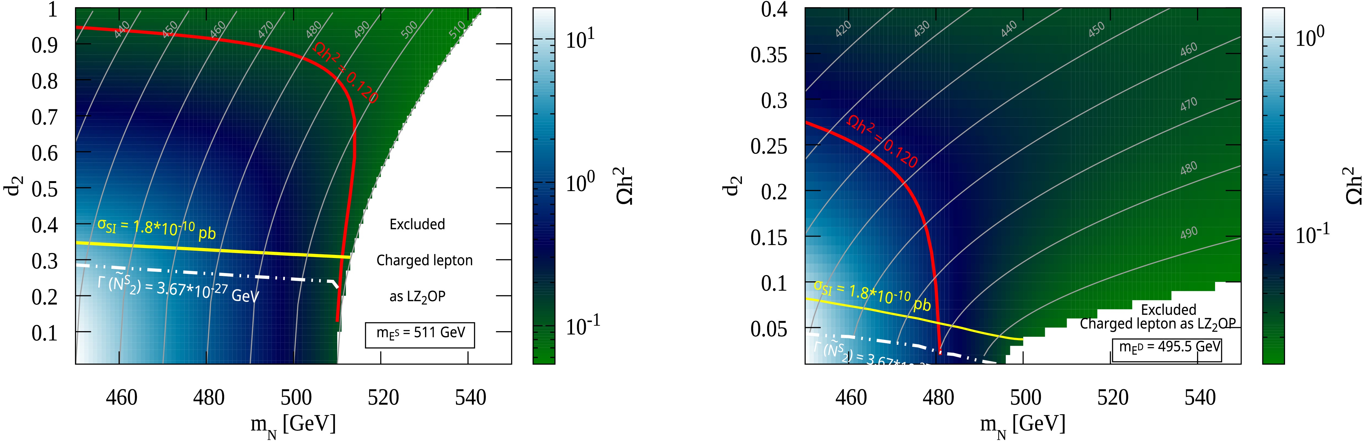
Figure 6. (color online) Relic density of the lightest exotic neutral fermion as DM, as a function of mass parameter
$ \widetilde m_N $ and scaling factor$ d_2 $ of coupling$ z_{{LN}} $ . The scale on the right side of the plot measures the abundance throughout the plane. The figures correspond to MH1 (left) and MH2 (right), as per Tables 2 and 3. The dashed curves correspond to observational bounds viz.,$ \Omega h^2=0.120 \pm 0.001 $ [14] (red),$ \sigma_{SI}=1.8 \times 10^{-10} $ pb [123–124] (yellow) and$ \Gamma \; (\widetilde N^S_2) = 3.67 \times 10 ^ {-27} $ GeV (white). The allowed regions are explained in the text. The region in white is excluded as charged lepton becomes the L$ Z_2 $ OP.● In the
$ \widetilde m_N \lt \widetilde m_L $ region: The DM is$ \widetilde N^S $ i.e., dominantly a singlet. As$ \widetilde m_N $ increases, the splitting$ | \widetilde m_L- \widetilde m_N| $ decreases, and the doublet component in DM increases. Concurrently, as$ d_2 $ ($ z_{{LN}} $ ) increases, the doublet component in the singlet-DM increases.● In the
$ \widetilde m_N \gt \widetilde m_L $ region: The DM is$ \widetilde N^D $ i.e., dominantly a doublet. As$ \widetilde m_N $ increases, the splitting$ | \widetilde m_L- \widetilde m_N| $ increases, and the doublet component in DM increases further. Concurrently, as$ d_2 $ ($ z_{{LN}} $ ) increases, the singlet component in the doublet-DM increases.This is indeed what we observe for both the plots in Fig. 6. Since the doublet component causes the DM to annihilate more, the relic density is maximum for the bottom left corner in the region
$ \widetilde m_N \lt \widetilde m_L $ and minimum for the bottom right corner in the region$ \widetilde m_N \gt \widetilde m_L $ . The white region is where the lightest$ Z_2 $ -odd particle is charged and therefore excluded from the feasible region.The set of points satisfying the relic density value of
$ \Omega h^2=0.120 $ are shown by the dashed curves in red. For the two different scenarios depicted here, the shapes of the relic density curves have a common interpretation. In the regions of small$ d_2 $ ($ z_{{LN}} $ ) and small$ \widetilde m_N $ ($ \widetilde m_N \lt \widetilde m_L $ ), the DM is strictly a singlet and, therefore, over-abundant in the absence of any considerable interactions. An increase in$ d_2 $ ($ z_{{LN}} $ ) as well as$ \widetilde m_N $ increases the doublet component in DM and therefore enhances its annihilations through a stronger coupling with the Z boson. However, an increase in$ \widetilde m_N $ also leads to coannihilations with other$ Z_2 $ -odd particles ($ \widetilde E^S $ ,$ \widetilde E^D $ ,$ \widetilde N^D $ or Φ's), which become increasingly efficient with the decrease in splitting$ | \widetilde m_N- \widetilde m_L| $ , whereas the decay of heavier species to DM becomes less efficient. These together lead to an over-decrease in DM density, which is avoided by a sharply decreasing singlet-doublet coupling$ d_2 $ ($ z_{{LN}} $ ) for large$ \widetilde m_N $ . This explains why the relic density is satisfied for a higher value of$ d_2 $ ($ z_{{LN}} $ ) at low values of$ \widetilde m_N $ and an almost vertically falling relic density curve as higher values of$ \widetilde m_N $ are approached. In brief, the DM relic abundance can be determined either via sizeable self-annihilation cross-sections—requiring a large$ d_2 $ ($ z_{{LN}} $ )—or through coannihilation processes involving heavier states.The qualitative differences between the two figures can be understood as follows.
Mass hierarchy-1 (MH1): This scenario is depicted in Fig. 6 (left). The relevant mass parameters other than
$ \widetilde m_N $ are$ \widetilde m_E=600 $ GeV,$ \mu_{\Phi}=650 $ GeV, and$ \widetilde m_L=850 $ GeV. The lightest$ Z_2 $ -odd charged particle (L$ Z_2 $ OCP) is$ \widetilde E^S $ with$ m_{ \widetilde E^S} \sim 511 $ GeV. The part of the plane is excluded where the$ \widetilde m_N $ value is such that$ \widetilde E^S $ becomes the L$ Z_2 $ OP (shown as white region in the plot). Thus,$ \widetilde m_N $ is varied in the range$ 450-550 $ GeV (for a given$ \widetilde m_N $ , the mass of DM decreases with an increase in$ d_2 $ ($ z_{{LN}} $ )). Since$ \widetilde m_L \sim 850 $ GeV, the DM is dominantly singlet ($ \widetilde N^S $ ) in the whole of the depicted plane. At$ \widetilde m_N \sim \widetilde m_E $ , the DM co-annihilates with the next heavier state,$ \widetilde E^S $ , and gets a contribution from its decays as well. The DM self-annihilations are quite suppressed, and the annihilations of$ \widetilde E^S $ determine the relic density. From Table 2, we observe that$ \widetilde E^S $ has a large doublet component due to large$ z_{{RE}} $ . Consequently, the dominant channel for relic density is$ \bar{ \widetilde E^S} \widetilde E^S \to W^+ W^- $ . In addition to the s-channel process, the process via t-channel vector-like leptons contributes significantly to this channel due to the large multiplicity of these mediators.Mass hierarchy-2 (MH2): This scenario is depicted in Fig. 6 (right). The values of the other relevant mass parameters are
$ \widetilde m_L=500 $ GeV,$ \widetilde m_E=1100 $ GeV, and$ \mu_{\Phi}=1200 $ GeV. Here, the L$ Z_2 $ OCP is a doublet,$ \widetilde E^D $ , with$ m_{ \widetilde E^D} \sim 496 $ GeV. Again,$ \widetilde m_N $ is varied in the range$ 450-550 $ GeV. The region where$ m_{ \widetilde N^D} $ exceeds$ m_{ \widetilde E^D} $ is excluded. Unlike MH1, the plane here is divided into two regions, viz.,$ \widetilde m_N \lt \widetilde m_L $ and$ \widetilde m_N \gt \widetilde m_L $ , although the curve explaining the observed value of relic density falls within the region$ \widetilde m_N \lt \widetilde m_L $ . As a result, the DM is again singlet-dominated. However, for a given$ \widetilde m_N $ and$ d_2 $ ($ z_{{LN}} $ ), the DM in this scenario has a smaller mass-splitting$ | \widetilde m_N- \widetilde m_L| $ and therefore, a larger doublet component compared to DM of Fig. 6 (left).The coannihilating partners of this DM are
$ \widetilde N^D $ and$ \widetilde E^D $ . From Tables 2 and 3, we observe that the scenario for MH2 admits relatively large values for the Yukawa couplings involving two vector-like leptons, viz.,$ y_{{lE}} $ and$ y_{{eL}} $ . Consequently, the dominant co-annihilating processes for DM occur via inert scalars in the t-channel. Following the specific structure of these Yukawa couplings, the dominant processes are$ \bar{ \widetilde E^D} \widetilde E^D \to \mu^+ \mu^- $ and$ \bar{ \widetilde N^D} \widetilde N^D \to \mu^+ \mu^- $ . The coannihilations in this scenario are much more efficient than those in MH1, as depicted by the relic density curve falling much before the excluded region in white. Further, the values of$ d_2 $ ($ z_{{LN}} $ ) satisfying the relic density are also significantly lower than those in the MH1. It may be noted that the region to the right of the relic density curve in red is under-abundant and, therefore, in principle, allowed unless excluded by charged lepton as the L$ Z_2 $ OP.Thus, from Fig. 6, we see how the relic density of dark matter is satisfied for two very different mass hierarchies in this model.
Constraints: It must be noted that for the two scenarios presented here, the output Yukawa couplings
$ y_{{lN}} $ ,$ y_{{eL}} $ , and$ z_{{LN}} $ were determined as per equations (32), (47), and (54) such that the various low energy observables (Secs. IV and V) are explained by default. Nevertheless, the values of these observables were computed numerically and it was found that in the whole plane of$ (\widetilde m_N,d_2) $ , as shown in Fig. 6 (left and right), the anomalies in electron and muon$ g-2 $ were explained while the various cLFV processes were within the experimental bounds. In addition, there are cosmological constraints as well as constraints from direct detection of dark matter, which are discussed in the following subsections. -
The thermal relic abundance of DM is governed by the Boltzmann equation, which describes the evolution of its number density as a function of its various interactions, as well as the universe's expansion. Considering the large spectrum of
$ Z_2 $ -odd particles, the DM relic abundance receives contributions not only from its annihilations but also from the annihilation of heavier particles that subsequently decay to DM. This process is called coannihilation, and it is relevant provided the mass difference between the DM and the heavier species is small. The corresponding Boltzmann equation is [121],$ \begin{aligned}[b] \frac{{\rm d}n_i}{{\rm d}t} =\;& -3 H n_i - \sum_{i,j=1}^N \langle \sigma_{ij}v_{ij}\rangle \left(n_in_j-n_i^{eq}n_j^{eq}\right) \\ & -\sum_{j\neq i} \Big[\langle{\sigma'}_{X_{ij}}v_{ij}\rangle \left(n_in_X-n_i^{eq}n_X^{eq}\right) \\&- \langle{\sigma'}_{X_{ji}}v_{ij}\rangle \left(n_jn_X-n_j^{eq}n_X^{eq}\right)\Big] \\ & -\sum_{j\neq i} \left[\Gamma_{ij} \left(n_i-n_i^{eq}\right) - \Gamma_{ji} \left(n_j-n_j^{eq}\right)\right], \end{aligned} $
(58) where
$ n_i $ denotes the number density of DM or one of the coannihilating species. There will be one such equation for each of the coannihilating species, including DM. Denoting$ Z_2 $ -odd particles by$ \chi_{i,j} $ and SM particles by$ X,Y $ , the terms other than the Hubble expansion term correspond to annihilations$ \chi_i\chi_j \to X X $ ,$ \chi_i $ to$ \chi_j $ conversion via scatterings$ \chi_iX \to \chi_j Y $ , and decays$ \chi_i \to \chi_j X $ , respectively. Other symbols are as follows:$ \langle \sigma v\rangle $ denotes the thermally averaged cross-section, subscript `$ eq $ ' denotes equilibrium, and H is the Hubble parameter. The processes leading to DM annihilation as well as coannihilation in the present model can be classified as● Annihilations to SM fermions, gauge bosons, or Higgs via s-channel mediation by SM gauge bosons or Higgs.
● Annihilations to SM fermions via t-channel exchange of inert scalars.
● Annihilations to SM bosons via t-channel mediation by
$ Z_2 $ -odd leptons.The gauge coupling with the Z-boson turns out to be the most critical in the annihilation process, affected through the doublet component in DM. This is why the singlet-doublet mixing of DM is crucial. On the other hand, the Yukawa couplings
$ y_{{lN}} $ ,$ y_{{lE}} $ , or$ y_{{eL}} $ affect only a few t-channel mediated processes and thus, are less significant. The relic abundance of DM is evaluated numerically using${\mathrm{micrOMEGAs}}$ [122]. It was found that the normal and inverted hierarchies with respect to the neutrino masses do not lead to qualitatively different results for dark matter. Henceforth, we discuss our results with respect to the normal hierarchy only. The effect of varying$ \widetilde m_N $ and$ d_2 $ ($ z_{{LN}} $ ) around the parameter points MH1 and MH2 on dark matter relic density and other related observables is depicted in Fig. 6, left and right, respectively. The other important parameter for dark matter study viz.,$ \widetilde m_L $ is fixed in these plots ($ 850 $ GeV for MH1 and$ 500 $ GeV for MH2). The value of$ \widetilde m_N $ relative to the fixed parameter$ \widetilde m_L $ impacts the nature of DM. To understand this, we consider the mixings of the$ Z_2 $ -odd neutral fermions given by equations (17) and (19). Following that, we see
Figure 6. (color online) Relic density of the lightest exotic neutral fermion as DM, as a function of mass parameter
$ \widetilde m_N $ and scaling factor$ d_2 $ of coupling$ z_{{LN}} $ . The scale on the right side of the plot measures the abundance throughout the plane. The figures correspond to MH1 (left) and MH2 (right), as per Tables 2 and 3. The dashed curves correspond to observational bounds viz.,$ \Omega h^2=0.120 \pm 0.001 $ [14] (red),$ \sigma_{SI}=1.8 \times 10^{-10} $ pb [123–124] (yellow) and$ \Gamma \; (\widetilde N^S_2) = 3.67 \times 10 ^ {-27} $ GeV (white). The allowed regions are explained in the text. The region in white is excluded as charged lepton becomes the L$ Z_2 $ OP.● In the
$ \widetilde m_N \lt \widetilde m_L $ region: The DM is$ \widetilde N^S $ i.e., dominantly a singlet. As$ \widetilde m_N $ increases, the splitting$ | \widetilde m_L- \widetilde m_N| $ decreases, and the doublet component in DM increases. Concurrently, as$ d_2 $ ($ z_{{LN}} $ ) increases, the doublet component in the singlet-DM increases.● In the
$ \widetilde m_N \gt \widetilde m_L $ region: The DM is$ \widetilde N^D $ i.e., dominantly a doublet. As$ \widetilde m_N $ increases, the splitting$ | \widetilde m_L- \widetilde m_N| $ increases, and the doublet component in DM increases further. Concurrently, as$ d_2 $ ($ z_{{LN}} $ ) increases, the singlet component in the doublet-DM increases.This is indeed what we observe for both the plots in Fig. 6. Since the doublet component causes the DM to annihilate more, the relic density is maximum for the bottom left corner in the region
$ \widetilde m_N \lt \widetilde m_L $ and minimum for the bottom right corner in the region$ \widetilde m_N \gt \widetilde m_L $ . The white region is where the lightest$ Z_2 $ -odd particle is charged and therefore excluded from the feasible region.The set of points satisfying the relic density value of
$ \Omega h^2=0.120 $ are shown by the dashed curves in red. For the two different scenarios depicted here, the shapes of the relic density curves have a common interpretation. In the regions of small$ d_2 $ ($ z_{{LN}} $ ) and small$ \widetilde m_N $ ($ \widetilde m_N \lt \widetilde m_L $ ), the DM is strictly a singlet and, therefore, over-abundant in the absence of any considerable interactions. An increase in$ d_2 $ ($ z_{{LN}} $ ) as well as$ \widetilde m_N $ increases the doublet component in DM and therefore enhances its annihilations through a stronger coupling with the Z boson. However, an increase in$ \widetilde m_N $ also leads to coannihilations with other$ Z_2 $ -odd particles ($ \widetilde E^S $ ,$ \widetilde E^D $ ,$ \widetilde N^D $ or Φ's), which become increasingly efficient with the decrease in splitting$ | \widetilde m_N- \widetilde m_L| $ , whereas the decay of heavier species to DM becomes less efficient. These together lead to an over-decrease in DM density, which is avoided by a sharply decreasing singlet-doublet coupling$ d_2 $ ($ z_{{LN}} $ ) for large$ \widetilde m_N $ . This explains why the relic density is satisfied for a higher value of$ d_2 $ ($ z_{{LN}} $ ) at low values of$ \widetilde m_N $ and an almost vertically falling relic density curve as higher values of$ \widetilde m_N $ are approached. In brief, the DM relic abundance can be determined either via sizeable self-annihilation cross-sections—requiring a large$ d_2 $ ($ z_{{LN}} $ )—or through coannihilation processes involving heavier states.The qualitative differences between the two figures can be understood as follows.
Mass hierarchy-1 (MH1): This scenario is depicted in Fig. 6 (left). The relevant mass parameters other than
$ \widetilde m_N $ are$ \widetilde m_E=600 $ GeV,$ \mu_{\Phi}=650 $ GeV, and$ \widetilde m_L=850 $ GeV. The lightest$ Z_2 $ -odd charged particle (L$ Z_2 $ OCP) is$ \widetilde E^S $ with$ m_{ \widetilde E^S} \sim 511 $ GeV. The part of the plane is excluded where the$ \widetilde m_N $ value is such that$ \widetilde E^S $ becomes the L$ Z_2 $ OP (shown as white region in the plot). Thus,$ \widetilde m_N $ is varied in the range$ 450-550 $ GeV (for a given$ \widetilde m_N $ , the mass of DM decreases with an increase in$ d_2 $ ($ z_{{LN}} $ )). Since$ \widetilde m_L \sim 850 $ GeV, the DM is dominantly singlet ($ \widetilde N^S $ ) in the whole of the depicted plane. At$ \widetilde m_N \sim \widetilde m_E $ , the DM co-annihilates with the next heavier state,$ \widetilde E^S $ , and gets a contribution from its decays as well. The DM self-annihilations are quite suppressed, and the annihilations of$ \widetilde E^S $ determine the relic density. From Table 2, we observe that$ \widetilde E^S $ has a large doublet component due to large$ z_{{RE}} $ . Consequently, the dominant channel for relic density is$ \bar{ \widetilde E^S} \widetilde E^S \to W^+ W^- $ . In addition to the s-channel process, the process via t-channel vector-like leptons contributes significantly to this channel due to the large multiplicity of these mediators.Mass hierarchy-2 (MH2): This scenario is depicted in Fig. 6 (right). The values of the other relevant mass parameters are
$ \widetilde m_L=500 $ GeV,$ \widetilde m_E=1100 $ GeV, and$ \mu_{\Phi}=1200 $ GeV. Here, the L$ Z_2 $ OCP is a doublet,$ \widetilde E^D $ , with$ m_{ \widetilde E^D} \sim 496 $ GeV. Again,$ \widetilde m_N $ is varied in the range$ 450-550 $ GeV. The region where$ m_{ \widetilde N^D} $ exceeds$ m_{ \widetilde E^D} $ is excluded. Unlike MH1, the plane here is divided into two regions, viz.,$ \widetilde m_N \lt \widetilde m_L $ and$ \widetilde m_N \gt \widetilde m_L $ , although the curve explaining the observed value of relic density falls within the region$ \widetilde m_N \lt \widetilde m_L $ . As a result, the DM is again singlet-dominated. However, for a given$ \widetilde m_N $ and$ d_2 $ ($ z_{{LN}} $ ), the DM in this scenario has a smaller mass-splitting$ | \widetilde m_N- \widetilde m_L| $ and therefore, a larger doublet component compared to DM of Fig. 6 (left).The coannihilating partners of this DM are
$ \widetilde N^D $ and$ \widetilde E^D $ . From Tables 2 and 3, we observe that the scenario for MH2 admits relatively large values for the Yukawa couplings involving two vector-like leptons, viz.,$ y_{{lE}} $ and$ y_{{eL}} $ . Consequently, the dominant co-annihilating processes for DM occur via inert scalars in the t-channel. Following the specific structure of these Yukawa couplings, the dominant processes are$ \bar{ \widetilde E^D} \widetilde E^D \to \mu^+ \mu^- $ and$ \bar{ \widetilde N^D} \widetilde N^D \to \mu^+ \mu^- $ . The coannihilations in this scenario are much more efficient than those in MH1, as depicted by the relic density curve falling much before the excluded region in white. Further, the values of$ d_2 $ ($ z_{{LN}} $ ) satisfying the relic density are also significantly lower than those in the MH1. It may be noted that the region to the right of the relic density curve in red is under-abundant and, therefore, in principle, allowed unless excluded by charged lepton as the L$ Z_2 $ OP.Thus, from Fig. 6, we see how the relic density of dark matter is satisfied for two very different mass hierarchies in this model.
Constraints: It must be noted that for the two scenarios presented here, the output Yukawa couplings
$ y_{{lN}} $ ,$ y_{{eL}} $ , and$ z_{{LN}} $ were determined as per equations (32), (47), and (54) such that the various low energy observables (Secs. IV and V) are explained by default. Nevertheless, the values of these observables were computed numerically and it was found that in the whole plane of$ (\widetilde m_N,d_2) $ , as shown in Fig. 6 (left and right), the anomalies in electron and muon$ g-2 $ were explained while the various cLFV processes were within the experimental bounds. In addition, there are cosmological constraints as well as constraints from direct detection of dark matter, which are discussed in the following subsections. -
The thermal relic abundance of DM is governed by the Boltzmann equation, which describes the evolution of its number density as a function of its various interactions, as well as the universe's expansion. Considering the large spectrum of
$ Z_2 $ -odd particles, the DM relic abundance receives contributions not only from its annihilations but also from the annihilation of heavier particles that subsequently decay to DM. This process is called coannihilation, and it is relevant provided the mass difference between the DM and the heavier species is small. The corresponding Boltzmann equation is [121],$ \begin{aligned}[b] \frac{{\rm d}n_i}{{\rm d}t} =\;& -3 H n_i - \sum_{i,j=1}^N \langle \sigma_{ij}v_{ij}\rangle \left(n_in_j-n_i^{eq}n_j^{eq}\right) \\ & -\sum_{j\neq i} \Big[\langle{\sigma'}_{X_{ij}}v_{ij}\rangle \left(n_in_X-n_i^{eq}n_X^{eq}\right) \\&- \langle{\sigma'}_{X_{ji}}v_{ij}\rangle \left(n_jn_X-n_j^{eq}n_X^{eq}\right)\Big] \\ & -\sum_{j\neq i} \left[\Gamma_{ij} \left(n_i-n_i^{eq}\right) - \Gamma_{ji} \left(n_j-n_j^{eq}\right)\right], \end{aligned} $
(58) where
$ n_i $ denotes the number density of DM or one of the coannihilating species. There will be one such equation for each of the coannihilating species, including DM. Denoting$ Z_2 $ -odd particles by$ \chi_{i,j} $ and SM particles by$ X,Y $ , the terms other than the Hubble expansion term correspond to annihilations$ \chi_i\chi_j \to X X $ ,$ \chi_i $ to$ \chi_j $ conversion via scatterings$ \chi_iX \to \chi_j Y $ , and decays$ \chi_i \to \chi_j X $ , respectively. Other symbols are as follows:$ \langle \sigma v\rangle $ denotes the thermally averaged cross-section, subscript `$ eq $ ' denotes equilibrium, and H is the Hubble parameter. The processes leading to DM annihilation as well as coannihilation in the present model can be classified as● Annihilations to SM fermions, gauge bosons, or Higgs via s-channel mediation by SM gauge bosons or Higgs.
● Annihilations to SM fermions via t-channel exchange of inert scalars.
● Annihilations to SM bosons via t-channel mediation by
$ Z_2 $ -odd leptons.The gauge coupling with the Z-boson turns out to be the most critical in the annihilation process, affected through the doublet component in DM. This is why the singlet-doublet mixing of DM is crucial. On the other hand, the Yukawa couplings
$ y_{{lN}} $ ,$ y_{{lE}} $ , or$ y_{{eL}} $ affect only a few t-channel mediated processes and thus, are less significant. The relic abundance of DM is evaluated numerically using${\mathrm{micrOMEGAs}}$ [122]. It was found that the normal and inverted hierarchies with respect to the neutrino masses do not lead to qualitatively different results for dark matter. Henceforth, we discuss our results with respect to the normal hierarchy only. The effect of varying$ \widetilde m_N $ and$ d_2 $ ($ z_{{LN}} $ ) around the parameter points MH1 and MH2 on dark matter relic density and other related observables is depicted in Fig. 6, left and right, respectively. The other important parameter for dark matter study viz.,$ \widetilde m_L $ is fixed in these plots ($ 850 $ GeV for MH1 and$ 500 $ GeV for MH2). The value of$ \widetilde m_N $ relative to the fixed parameter$ \widetilde m_L $ impacts the nature of DM. To understand this, we consider the mixings of the$ Z_2 $ -odd neutral fermions given by equations (17) and (19). Following that, we see
Figure 6. (color online) Relic density of the lightest exotic neutral fermion as DM, as a function of mass parameter
$ \widetilde m_N $ and scaling factor$ d_2 $ of coupling$ z_{{LN}} $ . The scale on the right side of the plot measures the abundance throughout the plane. The figures correspond to MH1 (left) and MH2 (right), as per Tables 2 and 3. The dashed curves correspond to observational bounds viz.,$ \Omega h^2=0.120 \pm 0.001 $ [14] (red),$ \sigma_{SI}=1.8 \times 10^{-10} $ pb [123–124] (yellow) and$ \Gamma \; (\widetilde N^S_2) = 3.67 \times 10 ^ {-27} $ GeV (white). The allowed regions are explained in the text. The region in white is excluded as charged lepton becomes the L$ Z_2 $ OP.● In the
$ \widetilde m_N \lt \widetilde m_L $ region: The DM is$ \widetilde N^S $ i.e., dominantly a singlet. As$ \widetilde m_N $ increases, the splitting$ | \widetilde m_L- \widetilde m_N| $ decreases, and the doublet component in DM increases. Concurrently, as$ d_2 $ ($ z_{{LN}} $ ) increases, the doublet component in the singlet-DM increases.● In the
$ \widetilde m_N \gt \widetilde m_L $ region: The DM is$ \widetilde N^D $ i.e., dominantly a doublet. As$ \widetilde m_N $ increases, the splitting$ | \widetilde m_L- \widetilde m_N| $ increases, and the doublet component in DM increases further. Concurrently, as$ d_2 $ ($ z_{{LN}} $ ) increases, the singlet component in the doublet-DM increases.This is indeed what we observe for both the plots in Fig. 6. Since the doublet component causes the DM to annihilate more, the relic density is maximum for the bottom left corner in the region
$ \widetilde m_N \lt \widetilde m_L $ and minimum for the bottom right corner in the region$ \widetilde m_N \gt \widetilde m_L $ . The white region is where the lightest$ Z_2 $ -odd particle is charged and therefore excluded from the feasible region.The set of points satisfying the relic density value of
$ \Omega h^2=0.120 $ are shown by the dashed curves in red. For the two different scenarios depicted here, the shapes of the relic density curves have a common interpretation. In the regions of small$ d_2 $ ($ z_{{LN}} $ ) and small$ \widetilde m_N $ ($ \widetilde m_N \lt \widetilde m_L $ ), the DM is strictly a singlet and, therefore, over-abundant in the absence of any considerable interactions. An increase in$ d_2 $ ($ z_{{LN}} $ ) as well as$ \widetilde m_N $ increases the doublet component in DM and therefore enhances its annihilations through a stronger coupling with the Z boson. However, an increase in$ \widetilde m_N $ also leads to coannihilations with other$ Z_2 $ -odd particles ($ \widetilde E^S $ ,$ \widetilde E^D $ ,$ \widetilde N^D $ or Φ's), which become increasingly efficient with the decrease in splitting$ | \widetilde m_N- \widetilde m_L| $ , whereas the decay of heavier species to DM becomes less efficient. These together lead to an over-decrease in DM density, which is avoided by a sharply decreasing singlet-doublet coupling$ d_2 $ ($ z_{{LN}} $ ) for large$ \widetilde m_N $ . This explains why the relic density is satisfied for a higher value of$ d_2 $ ($ z_{{LN}} $ ) at low values of$ \widetilde m_N $ and an almost vertically falling relic density curve as higher values of$ \widetilde m_N $ are approached. In brief, the DM relic abundance can be determined either via sizeable self-annihilation cross-sections—requiring a large$ d_2 $ ($ z_{{LN}} $ )—or through coannihilation processes involving heavier states.The qualitative differences between the two figures can be understood as follows.
Mass hierarchy-1 (MH1): This scenario is depicted in Fig. 6 (left). The relevant mass parameters other than
$ \widetilde m_N $ are$ \widetilde m_E=600 $ GeV,$ \mu_{\Phi}=650 $ GeV, and$ \widetilde m_L=850 $ GeV. The lightest$ Z_2 $ -odd charged particle (L$ Z_2 $ OCP) is$ \widetilde E^S $ with$ m_{ \widetilde E^S} \sim 511 $ GeV. The part of the plane is excluded where the$ \widetilde m_N $ value is such that$ \widetilde E^S $ becomes the L$ Z_2 $ OP (shown as white region in the plot). Thus,$ \widetilde m_N $ is varied in the range$ 450-550 $ GeV (for a given$ \widetilde m_N $ , the mass of DM decreases with an increase in$ d_2 $ ($ z_{{LN}} $ )). Since$ \widetilde m_L \sim 850 $ GeV, the DM is dominantly singlet ($ \widetilde N^S $ ) in the whole of the depicted plane. At$ \widetilde m_N \sim \widetilde m_E $ , the DM co-annihilates with the next heavier state,$ \widetilde E^S $ , and gets a contribution from its decays as well. The DM self-annihilations are quite suppressed, and the annihilations of$ \widetilde E^S $ determine the relic density. From Table 2, we observe that$ \widetilde E^S $ has a large doublet component due to large$ z_{{RE}} $ . Consequently, the dominant channel for relic density is$ \bar{ \widetilde E^S} \widetilde E^S \to W^+ W^- $ . In addition to the s-channel process, the process via t-channel vector-like leptons contributes significantly to this channel due to the large multiplicity of these mediators.Mass hierarchy-2 (MH2): This scenario is depicted in Fig. 6 (right). The values of the other relevant mass parameters are
$ \widetilde m_L=500 $ GeV,$ \widetilde m_E=1100 $ GeV, and$ \mu_{\Phi}=1200 $ GeV. Here, the L$ Z_2 $ OCP is a doublet,$ \widetilde E^D $ , with$ m_{ \widetilde E^D} \sim 496 $ GeV. Again,$ \widetilde m_N $ is varied in the range$ 450-550 $ GeV. The region where$ m_{ \widetilde N^D} $ exceeds$ m_{ \widetilde E^D} $ is excluded. Unlike MH1, the plane here is divided into two regions, viz.,$ \widetilde m_N \lt \widetilde m_L $ and$ \widetilde m_N \gt \widetilde m_L $ , although the curve explaining the observed value of relic density falls within the region$ \widetilde m_N \lt \widetilde m_L $ . As a result, the DM is again singlet-dominated. However, for a given$ \widetilde m_N $ and$ d_2 $ ($ z_{{LN}} $ ), the DM in this scenario has a smaller mass-splitting$ | \widetilde m_N- \widetilde m_L| $ and therefore, a larger doublet component compared to DM of Fig. 6 (left).The coannihilating partners of this DM are
$ \widetilde N^D $ and$ \widetilde E^D $ . From Tables 2 and 3, we observe that the scenario for MH2 admits relatively large values for the Yukawa couplings involving two vector-like leptons, viz.,$ y_{{lE}} $ and$ y_{{eL}} $ . Consequently, the dominant co-annihilating processes for DM occur via inert scalars in the t-channel. Following the specific structure of these Yukawa couplings, the dominant processes are$ \bar{ \widetilde E^D} \widetilde E^D \to \mu^+ \mu^- $ and$ \bar{ \widetilde N^D} \widetilde N^D \to \mu^+ \mu^- $ . The coannihilations in this scenario are much more efficient than those in MH1, as depicted by the relic density curve falling much before the excluded region in white. Further, the values of$ d_2 $ ($ z_{{LN}} $ ) satisfying the relic density are also significantly lower than those in the MH1. It may be noted that the region to the right of the relic density curve in red is under-abundant and, therefore, in principle, allowed unless excluded by charged lepton as the L$ Z_2 $ OP.Thus, from Fig. 6, we see how the relic density of dark matter is satisfied for two very different mass hierarchies in this model.
Constraints: It must be noted that for the two scenarios presented here, the output Yukawa couplings
$ y_{{lN}} $ ,$ y_{{eL}} $ , and$ z_{{LN}} $ were determined as per equations (32), (47), and (54) such that the various low energy observables (Secs. IV and V) are explained by default. Nevertheless, the values of these observables were computed numerically and it was found that in the whole plane of$ (\widetilde m_N,d_2) $ , as shown in Fig. 6 (left and right), the anomalies in electron and muon$ g-2 $ were explained while the various cLFV processes were within the experimental bounds. In addition, there are cosmological constraints as well as constraints from direct detection of dark matter, which are discussed in the following subsections. -
The thermal relic abundance of DM is governed by the Boltzmann equation, which describes the evolution of its number density as a function of its various interactions, as well as the universe's expansion. Considering the large spectrum of
$ Z_2 $ -odd particles, the DM relic abundance receives contributions not only from its annihilations but also from the annihilation of heavier particles that subsequently decay to DM. This process is called coannihilation, and it is relevant provided the mass difference between the DM and the heavier species is small. The corresponding Boltzmann equation is [121],$ \begin{aligned}[b] \frac{{\rm d}n_i}{{\rm d}t} =\;& -3 H n_i - \sum_{i,j=1}^N \langle \sigma_{ij}v_{ij}\rangle \left(n_in_j-n_i^{eq}n_j^{eq}\right) \\ & -\sum_{j\neq i} \Big[\langle{\sigma'}_{X_{ij}}v_{ij}\rangle \left(n_in_X-n_i^{eq}n_X^{eq}\right) \\&- \langle{\sigma'}_{X_{ji}}v_{ij}\rangle \left(n_jn_X-n_j^{eq}n_X^{eq}\right)\Big] \\ & -\sum_{j\neq i} \left[\Gamma_{ij} \left(n_i-n_i^{eq}\right) - \Gamma_{ji} \left(n_j-n_j^{eq}\right)\right], \end{aligned} $
(58) where
$ n_i $ denotes the number density of DM or one of the coannihilating species. There will be one such equation for each of the coannihilating species, including DM. Denoting$ Z_2 $ -odd particles by$ \chi_{i,j} $ and SM particles by$ X,Y $ , the terms other than the Hubble expansion term correspond to annihilations$ \chi_i\chi_j \to X X $ ,$ \chi_i $ to$ \chi_j $ conversion via scatterings$ \chi_iX \to \chi_j Y $ , and decays$ \chi_i \to \chi_j X $ , respectively. Other symbols are as follows:$ \langle \sigma v\rangle $ denotes the thermally averaged cross-section, subscript `$ eq $ ' denotes equilibrium, and H is the Hubble parameter. The processes leading to DM annihilation as well as coannihilation in the present model can be classified as● Annihilations to SM fermions, gauge bosons, or Higgs via s-channel mediation by SM gauge bosons or Higgs.
● Annihilations to SM fermions via t-channel exchange of inert scalars.
● Annihilations to SM bosons via t-channel mediation by
$ Z_2 $ -odd leptons.The gauge coupling with the Z-boson turns out to be the most critical in the annihilation process, affected through the doublet component in DM. This is why the singlet-doublet mixing of DM is crucial. On the other hand, the Yukawa couplings
$ y_{{lN}} $ ,$ y_{{lE}} $ , or$ y_{{eL}} $ affect only a few t-channel mediated processes and thus, are less significant. The relic abundance of DM is evaluated numerically using${\mathrm{micrOMEGAs}}$ [122]. It was found that the normal and inverted hierarchies with respect to the neutrino masses do not lead to qualitatively different results for dark matter. Henceforth, we discuss our results with respect to the normal hierarchy only. The effect of varying$ \widetilde m_N $ and$ d_2 $ ($ z_{{LN}} $ ) around the parameter points MH1 and MH2 on dark matter relic density and other related observables is depicted in Fig. 6, left and right, respectively. The other important parameter for dark matter study viz.,$ \widetilde m_L $ is fixed in these plots ($ 850 $ GeV for MH1 and$ 500 $ GeV for MH2). The value of$ \widetilde m_N $ relative to the fixed parameter$ \widetilde m_L $ impacts the nature of DM. To understand this, we consider the mixings of the$ Z_2 $ -odd neutral fermions given by equations (17) and (19). Following that, we see
Figure 6. (color online) Relic density of the lightest exotic neutral fermion as DM, as a function of mass parameter
$ \widetilde m_N $ and scaling factor$ d_2 $ of coupling$ z_{{LN}} $ . The scale on the right side of the plot measures the abundance throughout the plane. The figures correspond to MH1 (left) and MH2 (right), as per Tables 2 and 3. The dashed curves correspond to observational bounds viz.,$ \Omega h^2=0.120 \pm 0.001 $ [14] (red),$ \sigma_{SI}=1.8 \times 10^{-10} $ pb [123–124] (yellow) and$ \Gamma \; (\widetilde N^S_2) = 3.67 \times 10 ^ {-27} $ GeV (white). The allowed regions are explained in the text. The region in white is excluded as charged lepton becomes the L$ Z_2 $ OP.● In the
$ \widetilde m_N \lt \widetilde m_L $ region: The DM is$ \widetilde N^S $ i.e., dominantly a singlet. As$ \widetilde m_N $ increases, the splitting$ | \widetilde m_L- \widetilde m_N| $ decreases, and the doublet component in DM increases. Concurrently, as$ d_2 $ ($ z_{{LN}} $ ) increases, the doublet component in the singlet-DM increases.● In the
$ \widetilde m_N \gt \widetilde m_L $ region: The DM is$ \widetilde N^D $ i.e., dominantly a doublet. As$ \widetilde m_N $ increases, the splitting$ | \widetilde m_L- \widetilde m_N| $ increases, and the doublet component in DM increases further. Concurrently, as$ d_2 $ ($ z_{{LN}} $ ) increases, the singlet component in the doublet-DM increases.This is indeed what we observe for both the plots in Fig. 6. Since the doublet component causes the DM to annihilate more, the relic density is maximum for the bottom left corner in the region
$ \widetilde m_N \lt \widetilde m_L $ and minimum for the bottom right corner in the region$ \widetilde m_N \gt \widetilde m_L $ . The white region is where the lightest$ Z_2 $ -odd particle is charged and therefore excluded from the feasible region.The set of points satisfying the relic density value of
$ \Omega h^2=0.120 $ are shown by the dashed curves in red. For the two different scenarios depicted here, the shapes of the relic density curves have a common interpretation. In the regions of small$ d_2 $ ($ z_{{LN}} $ ) and small$ \widetilde m_N $ ($ \widetilde m_N \lt \widetilde m_L $ ), the DM is strictly a singlet and, therefore, over-abundant in the absence of any considerable interactions. An increase in$ d_2 $ ($ z_{{LN}} $ ) as well as$ \widetilde m_N $ increases the doublet component in DM and therefore enhances its annihilations through a stronger coupling with the Z boson. However, an increase in$ \widetilde m_N $ also leads to coannihilations with other$ Z_2 $ -odd particles ($ \widetilde E^S $ ,$ \widetilde E^D $ ,$ \widetilde N^D $ or Φ's), which become increasingly efficient with the decrease in splitting$ | \widetilde m_N- \widetilde m_L| $ , whereas the decay of heavier species to DM becomes less efficient. These together lead to an over-decrease in DM density, which is avoided by a sharply decreasing singlet-doublet coupling$ d_2 $ ($ z_{{LN}} $ ) for large$ \widetilde m_N $ . This explains why the relic density is satisfied for a higher value of$ d_2 $ ($ z_{{LN}} $ ) at low values of$ \widetilde m_N $ and an almost vertically falling relic density curve as higher values of$ \widetilde m_N $ are approached. In brief, the DM relic abundance can be determined either via sizeable self-annihilation cross-sections—requiring a large$ d_2 $ ($ z_{{LN}} $ )—or through coannihilation processes involving heavier states.The qualitative differences between the two figures can be understood as follows.
Mass hierarchy-1 (MH1): This scenario is depicted in Fig. 6 (left). The relevant mass parameters other than
$ \widetilde m_N $ are$ \widetilde m_E=600 $ GeV,$ \mu_{\Phi}=650 $ GeV, and$ \widetilde m_L=850 $ GeV. The lightest$ Z_2 $ -odd charged particle (L$ Z_2 $ OCP) is$ \widetilde E^S $ with$ m_{ \widetilde E^S} \sim 511 $ GeV. The part of the plane is excluded where the$ \widetilde m_N $ value is such that$ \widetilde E^S $ becomes the L$ Z_2 $ OP (shown as white region in the plot). Thus,$ \widetilde m_N $ is varied in the range$ 450-550 $ GeV (for a given$ \widetilde m_N $ , the mass of DM decreases with an increase in$ d_2 $ ($ z_{{LN}} $ )). Since$ \widetilde m_L \sim 850 $ GeV, the DM is dominantly singlet ($ \widetilde N^S $ ) in the whole of the depicted plane. At$ \widetilde m_N \sim \widetilde m_E $ , the DM co-annihilates with the next heavier state,$ \widetilde E^S $ , and gets a contribution from its decays as well. The DM self-annihilations are quite suppressed, and the annihilations of$ \widetilde E^S $ determine the relic density. From Table 2, we observe that$ \widetilde E^S $ has a large doublet component due to large$ z_{{RE}} $ . Consequently, the dominant channel for relic density is$ \bar{ \widetilde E^S} \widetilde E^S \to W^+ W^- $ . In addition to the s-channel process, the process via t-channel vector-like leptons contributes significantly to this channel due to the large multiplicity of these mediators.Mass hierarchy-2 (MH2): This scenario is depicted in Fig. 6 (right). The values of the other relevant mass parameters are
$ \widetilde m_L=500 $ GeV,$ \widetilde m_E=1100 $ GeV, and$ \mu_{\Phi}=1200 $ GeV. Here, the L$ Z_2 $ OCP is a doublet,$ \widetilde E^D $ , with$ m_{ \widetilde E^D} \sim 496 $ GeV. Again,$ \widetilde m_N $ is varied in the range$ 450-550 $ GeV. The region where$ m_{ \widetilde N^D} $ exceeds$ m_{ \widetilde E^D} $ is excluded. Unlike MH1, the plane here is divided into two regions, viz.,$ \widetilde m_N \lt \widetilde m_L $ and$ \widetilde m_N \gt \widetilde m_L $ , although the curve explaining the observed value of relic density falls within the region$ \widetilde m_N \lt \widetilde m_L $ . As a result, the DM is again singlet-dominated. However, for a given$ \widetilde m_N $ and$ d_2 $ ($ z_{{LN}} $ ), the DM in this scenario has a smaller mass-splitting$ | \widetilde m_N- \widetilde m_L| $ and therefore, a larger doublet component compared to DM of Fig. 6 (left).The coannihilating partners of this DM are
$ \widetilde N^D $ and$ \widetilde E^D $ . From Tables 2 and 3, we observe that the scenario for MH2 admits relatively large values for the Yukawa couplings involving two vector-like leptons, viz.,$ y_{{lE}} $ and$ y_{{eL}} $ . Consequently, the dominant co-annihilating processes for DM occur via inert scalars in the t-channel. Following the specific structure of these Yukawa couplings, the dominant processes are$ \bar{ \widetilde E^D} \widetilde E^D \to \mu^+ \mu^- $ and$ \bar{ \widetilde N^D} \widetilde N^D \to \mu^+ \mu^- $ . The coannihilations in this scenario are much more efficient than those in MH1, as depicted by the relic density curve falling much before the excluded region in white. Further, the values of$ d_2 $ ($ z_{{LN}} $ ) satisfying the relic density are also significantly lower than those in the MH1. It may be noted that the region to the right of the relic density curve in red is under-abundant and, therefore, in principle, allowed unless excluded by charged lepton as the L$ Z_2 $ OP.Thus, from Fig. 6, we see how the relic density of dark matter is satisfied for two very different mass hierarchies in this model.
Constraints: It must be noted that for the two scenarios presented here, the output Yukawa couplings
$ y_{{lN}} $ ,$ y_{{eL}} $ , and$ z_{{LN}} $ were determined as per equations (32), (47), and (54) such that the various low energy observables (Secs. IV and V) are explained by default. Nevertheless, the values of these observables were computed numerically and it was found that in the whole plane of$ (\widetilde m_N,d_2) $ , as shown in Fig. 6 (left and right), the anomalies in electron and muon$ g-2 $ were explained while the various cLFV processes were within the experimental bounds. In addition, there are cosmological constraints as well as constraints from direct detection of dark matter, which are discussed in the following subsections. -
The thermal relic abundance of DM is governed by the Boltzmann equation, which describes the evolution of its number density as a function of its various interactions, as well as the universe's expansion. Considering the large spectrum of
$ Z_2 $ -odd particles, the DM relic abundance receives contributions not only from its annihilations but also from the annihilation of heavier particles that subsequently decay to DM. This process is called coannihilation, and it is relevant provided the mass difference between the DM and the heavier species is small. The corresponding Boltzmann equation is [121],$ \begin{aligned}[b] \frac{{\rm d}n_i}{{\rm d}t} =\;& -3 H n_i - \sum_{i,j=1}^N \langle \sigma_{ij}v_{ij}\rangle \left(n_in_j-n_i^{eq}n_j^{eq}\right) \\ & -\sum_{j\neq i} \Big[\langle{\sigma'}_{X_{ij}}v_{ij}\rangle \left(n_in_X-n_i^{eq}n_X^{eq}\right) \\&- \langle{\sigma'}_{X_{ji}}v_{ij}\rangle \left(n_jn_X-n_j^{eq}n_X^{eq}\right)\Big] \\ & -\sum_{j\neq i} \left[\Gamma_{ij} \left(n_i-n_i^{eq}\right) - \Gamma_{ji} \left(n_j-n_j^{eq}\right)\right], \end{aligned} $
(58) where
$ n_i $ denotes the number density of DM or one of the coannihilating species. There will be one such equation for each of the coannihilating species, including DM. Denoting$ Z_2 $ -odd particles by$ \chi_{i,j} $ and SM particles by$ X,Y $ , the terms other than the Hubble expansion term correspond to annihilations$ \chi_i\chi_j \to X X $ ,$ \chi_i $ to$ \chi_j $ conversion via scatterings$ \chi_iX \to \chi_j Y $ , and decays$ \chi_i \to \chi_j X $ , respectively. Other symbols are as follows:$ \langle \sigma v\rangle $ denotes the thermally averaged cross-section, subscript `$ eq $ ' denotes equilibrium, and H is the Hubble parameter. The processes leading to DM annihilation as well as coannihilation in the present model can be classified as● Annihilations to SM fermions, gauge bosons, or Higgs via s-channel mediation by SM gauge bosons or Higgs.
● Annihilations to SM fermions via t-channel exchange of inert scalars.
● Annihilations to SM bosons via t-channel mediation by
$ Z_2 $ -odd leptons.The gauge coupling with the Z-boson turns out to be the most critical in the annihilation process, affected through the doublet component in DM. This is why the singlet-doublet mixing of DM is crucial. On the other hand, the Yukawa couplings
$ y_{{lN}} $ ,$ y_{{lE}} $ , or$ y_{{eL}} $ affect only a few t-channel mediated processes and thus, are less significant. The relic abundance of DM is evaluated numerically using${\mathrm{micrOMEGAs}}$ [122]. It was found that the normal and inverted hierarchies with respect to the neutrino masses do not lead to qualitatively different results for dark matter. Henceforth, we discuss our results with respect to the normal hierarchy only. The effect of varying$ \widetilde m_N $ and$ d_2 $ ($ z_{{LN}} $ ) around the parameter points MH1 and MH2 on dark matter relic density and other related observables is depicted in Fig. 6, left and right, respectively. The other important parameter for dark matter study viz.,$ \widetilde m_L $ is fixed in these plots ($ 850 $ GeV for MH1 and$ 500 $ GeV for MH2). The value of$ \widetilde m_N $ relative to the fixed parameter$ \widetilde m_L $ impacts the nature of DM. To understand this, we consider the mixings of the$ Z_2 $ -odd neutral fermions given by equations (17) and (19). Following that, we see
Figure 6. (color online) Relic density of the lightest exotic neutral fermion as DM, as a function of mass parameter
$ \widetilde m_N $ and scaling factor$ d_2 $ of coupling$ z_{{LN}} $ . The scale on the right side of the plot measures the abundance throughout the plane. The figures correspond to MH1 (left) and MH2 (right), as per Tables 2 and 3. The dashed curves correspond to observational bounds viz.,$ \Omega h^2=0.120 \pm 0.001 $ [14] (red),$ \sigma_{SI}=1.8 \times 10^{-10} $ pb [123–124] (yellow) and$ \Gamma \; (\widetilde N^S_2) = 3.67 \times 10 ^ {-27} $ GeV (white). The allowed regions are explained in the text. The region in white is excluded as charged lepton becomes the L$ Z_2 $ OP.● In the
$ \widetilde m_N \lt \widetilde m_L $ region: The DM is$ \widetilde N^S $ i.e., dominantly a singlet. As$ \widetilde m_N $ increases, the splitting$ | \widetilde m_L- \widetilde m_N| $ decreases, and the doublet component in DM increases. Concurrently, as$ d_2 $ ($ z_{{LN}} $ ) increases, the doublet component in the singlet-DM increases.● In the
$ \widetilde m_N \gt \widetilde m_L $ region: The DM is$ \widetilde N^D $ i.e., dominantly a doublet. As$ \widetilde m_N $ increases, the splitting$ | \widetilde m_L- \widetilde m_N| $ increases, and the doublet component in DM increases further. Concurrently, as$ d_2 $ ($ z_{{LN}} $ ) increases, the singlet component in the doublet-DM increases.This is indeed what we observe for both the plots in Fig. 6. Since the doublet component causes the DM to annihilate more, the relic density is maximum for the bottom left corner in the region
$ \widetilde m_N \lt \widetilde m_L $ and minimum for the bottom right corner in the region$ \widetilde m_N \gt \widetilde m_L $ . The white region is where the lightest$ Z_2 $ -odd particle is charged and therefore excluded from the feasible region.The set of points satisfying the relic density value of
$ \Omega h^2=0.120 $ are shown by the dashed curves in red. For the two different scenarios depicted here, the shapes of the relic density curves have a common interpretation. In the regions of small$ d_2 $ ($ z_{{LN}} $ ) and small$ \widetilde m_N $ ($ \widetilde m_N \lt \widetilde m_L $ ), the DM is strictly a singlet and, therefore, over-abundant in the absence of any considerable interactions. An increase in$ d_2 $ ($ z_{{LN}} $ ) as well as$ \widetilde m_N $ increases the doublet component in DM and therefore enhances its annihilations through a stronger coupling with the Z boson. However, an increase in$ \widetilde m_N $ also leads to coannihilations with other$ Z_2 $ -odd particles ($ \widetilde E^S $ ,$ \widetilde E^D $ ,$ \widetilde N^D $ or Φ's), which become increasingly efficient with the decrease in splitting$ | \widetilde m_N- \widetilde m_L| $ , whereas the decay of heavier species to DM becomes less efficient. These together lead to an over-decrease in DM density, which is avoided by a sharply decreasing singlet-doublet coupling$ d_2 $ ($ z_{{LN}} $ ) for large$ \widetilde m_N $ . This explains why the relic density is satisfied for a higher value of$ d_2 $ ($ z_{{LN}} $ ) at low values of$ \widetilde m_N $ and an almost vertically falling relic density curve as higher values of$ \widetilde m_N $ are approached. In brief, the DM relic abundance can be determined either via sizeable self-annihilation cross-sections—requiring a large$ d_2 $ ($ z_{{LN}} $ )—or through coannihilation processes involving heavier states.The qualitative differences between the two figures can be understood as follows.
Mass hierarchy-1 (MH1): This scenario is depicted in Fig. 6 (left). The relevant mass parameters other than
$ \widetilde m_N $ are$ \widetilde m_E=600 $ GeV,$ \mu_{\Phi}=650 $ GeV, and$ \widetilde m_L=850 $ GeV. The lightest$ Z_2 $ -odd charged particle (L$ Z_2 $ OCP) is$ \widetilde E^S $ with$ m_{ \widetilde E^S} \sim 511 $ GeV. The part of the plane is excluded where the$ \widetilde m_N $ value is such that$ \widetilde E^S $ becomes the L$ Z_2 $ OP (shown as white region in the plot). Thus,$ \widetilde m_N $ is varied in the range$ 450-550 $ GeV (for a given$ \widetilde m_N $ , the mass of DM decreases with an increase in$ d_2 $ ($ z_{{LN}} $ )). Since$ \widetilde m_L \sim 850 $ GeV, the DM is dominantly singlet ($ \widetilde N^S $ ) in the whole of the depicted plane. At$ \widetilde m_N \sim \widetilde m_E $ , the DM co-annihilates with the next heavier state,$ \widetilde E^S $ , and gets a contribution from its decays as well. The DM self-annihilations are quite suppressed, and the annihilations of$ \widetilde E^S $ determine the relic density. From Table 2, we observe that$ \widetilde E^S $ has a large doublet component due to large$ z_{{RE}} $ . Consequently, the dominant channel for relic density is$ \bar{ \widetilde E^S} \widetilde E^S \to W^+ W^- $ . In addition to the s-channel process, the process via t-channel vector-like leptons contributes significantly to this channel due to the large multiplicity of these mediators.Mass hierarchy-2 (MH2): This scenario is depicted in Fig. 6 (right). The values of the other relevant mass parameters are
$ \widetilde m_L=500 $ GeV,$ \widetilde m_E=1100 $ GeV, and$ \mu_{\Phi}=1200 $ GeV. Here, the L$ Z_2 $ OCP is a doublet,$ \widetilde E^D $ , with$ m_{ \widetilde E^D} \sim 496 $ GeV. Again,$ \widetilde m_N $ is varied in the range$ 450-550 $ GeV. The region where$ m_{ \widetilde N^D} $ exceeds$ m_{ \widetilde E^D} $ is excluded. Unlike MH1, the plane here is divided into two regions, viz.,$ \widetilde m_N \lt \widetilde m_L $ and$ \widetilde m_N \gt \widetilde m_L $ , although the curve explaining the observed value of relic density falls within the region$ \widetilde m_N \lt \widetilde m_L $ . As a result, the DM is again singlet-dominated. However, for a given$ \widetilde m_N $ and$ d_2 $ ($ z_{{LN}} $ ), the DM in this scenario has a smaller mass-splitting$ | \widetilde m_N- \widetilde m_L| $ and therefore, a larger doublet component compared to DM of Fig. 6 (left).The coannihilating partners of this DM are
$ \widetilde N^D $ and$ \widetilde E^D $ . From Tables 2 and 3, we observe that the scenario for MH2 admits relatively large values for the Yukawa couplings involving two vector-like leptons, viz.,$ y_{{lE}} $ and$ y_{{eL}} $ . Consequently, the dominant co-annihilating processes for DM occur via inert scalars in the t-channel. Following the specific structure of these Yukawa couplings, the dominant processes are$ \bar{ \widetilde E^D} \widetilde E^D \to \mu^+ \mu^- $ and$ \bar{ \widetilde N^D} \widetilde N^D \to \mu^+ \mu^- $ . The coannihilations in this scenario are much more efficient than those in MH1, as depicted by the relic density curve falling much before the excluded region in white. Further, the values of$ d_2 $ ($ z_{{LN}} $ ) satisfying the relic density are also significantly lower than those in the MH1. It may be noted that the region to the right of the relic density curve in red is under-abundant and, therefore, in principle, allowed unless excluded by charged lepton as the L$ Z_2 $ OP.Thus, from Fig. 6, we see how the relic density of dark matter is satisfied for two very different mass hierarchies in this model.
Constraints: It must be noted that for the two scenarios presented here, the output Yukawa couplings
$ y_{{lN}} $ ,$ y_{{eL}} $ , and$ z_{{LN}} $ were determined as per equations (32), (47), and (54) such that the various low energy observables (Secs. IV and V) are explained by default. Nevertheless, the values of these observables were computed numerically and it was found that in the whole plane of$ (\widetilde m_N,d_2) $ , as shown in Fig. 6 (left and right), the anomalies in electron and muon$ g-2 $ were explained while the various cLFV processes were within the experimental bounds. In addition, there are cosmological constraints as well as constraints from direct detection of dark matter, which are discussed in the following subsections. -
The thermal relic abundance of DM is governed by the Boltzmann equation, which describes the evolution of its number density as a function of its various interactions, as well as the universe's expansion. Considering the large spectrum of
$ Z_2 $ -odd particles, the DM relic abundance receives contributions not only from its annihilations but also from the annihilation of heavier particles that subsequently decay to DM. This process is called coannihilation, and it is relevant provided the mass difference between the DM and the heavier species is small. The corresponding Boltzmann equation is [121],$ \begin{aligned}[b] \frac{{\rm d}n_i}{{\rm d}t} =\;& -3 H n_i - \sum_{i,j=1}^N \langle \sigma_{ij}v_{ij}\rangle \left(n_in_j-n_i^{eq}n_j^{eq}\right) \\ & -\sum_{j\neq i} \Big[\langle{\sigma'}_{X_{ij}}v_{ij}\rangle \left(n_in_X-n_i^{eq}n_X^{eq}\right) \\&- \langle{\sigma'}_{X_{ji}}v_{ij}\rangle \left(n_jn_X-n_j^{eq}n_X^{eq}\right)\Big] \\ & -\sum_{j\neq i} \left[\Gamma_{ij} \left(n_i-n_i^{eq}\right) - \Gamma_{ji} \left(n_j-n_j^{eq}\right)\right], \end{aligned} $
(58) where
$ n_i $ denotes the number density of DM or one of the coannihilating species. There will be one such equation for each of the coannihilating species, including DM. Denoting$ Z_2 $ -odd particles by$ \chi_{i,j} $ and SM particles by$ X,Y $ , the terms other than the Hubble expansion term correspond to annihilations$ \chi_i\chi_j \to X X $ ,$ \chi_i $ to$ \chi_j $ conversion via scatterings$ \chi_iX \to \chi_j Y $ , and decays$ \chi_i \to \chi_j X $ , respectively. Other symbols are as follows:$ \langle \sigma v\rangle $ denotes the thermally averaged cross-section, subscript `$ eq $ ' denotes equilibrium, and H is the Hubble parameter. The processes leading to DM annihilation as well as coannihilation in the present model can be classified as● Annihilations to SM fermions, gauge bosons, or Higgs via s-channel mediation by SM gauge bosons or Higgs.
● Annihilations to SM fermions via t-channel exchange of inert scalars.
● Annihilations to SM bosons via t-channel mediation by
$ Z_2 $ -odd leptons.The gauge coupling with the Z-boson turns out to be the most critical in the annihilation process, affected through the doublet component in DM. This is why the singlet-doublet mixing of DM is crucial. On the other hand, the Yukawa couplings
$ y_{{lN}} $ ,$ y_{{lE}} $ , or$ y_{{eL}} $ affect only a few t-channel mediated processes and thus, are less significant. The relic abundance of DM is evaluated numerically using${\mathrm{micrOMEGAs}}$ [122]. It was found that the normal and inverted hierarchies with respect to the neutrino masses do not lead to qualitatively different results for dark matter. Henceforth, we discuss our results with respect to the normal hierarchy only. The effect of varying$ \widetilde m_N $ and$ d_2 $ ($ z_{{LN}} $ ) around the parameter points MH1 and MH2 on dark matter relic density and other related observables is depicted in Fig. 6, left and right, respectively. The other important parameter for dark matter study viz.,$ \widetilde m_L $ is fixed in these plots ($ 850 $ GeV for MH1 and$ 500 $ GeV for MH2). The value of$ \widetilde m_N $ relative to the fixed parameter$ \widetilde m_L $ impacts the nature of DM. To understand this, we consider the mixings of the$ Z_2 $ -odd neutral fermions given by equations (17) and (19). Following that, we see
Figure 6. (color online) Relic density of the lightest exotic neutral fermion as DM, as a function of mass parameter
$ \widetilde m_N $ and scaling factor$ d_2 $ of coupling$ z_{{LN}} $ . The scale on the right side of the plot measures the abundance throughout the plane. The figures correspond to MH1 (left) and MH2 (right), as per Tables 2 and 3. The dashed curves correspond to observational bounds viz.,$ \Omega h^2=0.120 \pm 0.001 $ [14] (red),$ \sigma_{SI}=1.8 \times 10^{-10} $ pb [123–124] (yellow) and$ \Gamma \; (\widetilde N^S_2) = 3.67 \times 10 ^ {-27} $ GeV (white). The allowed regions are explained in the text. The region in white is excluded as charged lepton becomes the L$ Z_2 $ OP.● In the
$ \widetilde m_N \lt \widetilde m_L $ region: The DM is$ \widetilde N^S $ i.e., dominantly a singlet. As$ \widetilde m_N $ increases, the splitting$ | \widetilde m_L- \widetilde m_N| $ decreases, and the doublet component in DM increases. Concurrently, as$ d_2 $ ($ z_{{LN}} $ ) increases, the doublet component in the singlet-DM increases.● In the
$ \widetilde m_N \gt \widetilde m_L $ region: The DM is$ \widetilde N^D $ i.e., dominantly a doublet. As$ \widetilde m_N $ increases, the splitting$ | \widetilde m_L- \widetilde m_N| $ increases, and the doublet component in DM increases further. Concurrently, as$ d_2 $ ($ z_{{LN}} $ ) increases, the singlet component in the doublet-DM increases.This is indeed what we observe for both the plots in Fig. 6. Since the doublet component causes the DM to annihilate more, the relic density is maximum for the bottom left corner in the region
$ \widetilde m_N \lt \widetilde m_L $ and minimum for the bottom right corner in the region$ \widetilde m_N \gt \widetilde m_L $ . The white region is where the lightest$ Z_2 $ -odd particle is charged and therefore excluded from the feasible region.The set of points satisfying the relic density value of
$ \Omega h^2=0.120 $ are shown by the dashed curves in red. For the two different scenarios depicted here, the shapes of the relic density curves have a common interpretation. In the regions of small$ d_2 $ ($ z_{{LN}} $ ) and small$ \widetilde m_N $ ($ \widetilde m_N \lt \widetilde m_L $ ), the DM is strictly a singlet and, therefore, over-abundant in the absence of any considerable interactions. An increase in$ d_2 $ ($ z_{{LN}} $ ) as well as$ \widetilde m_N $ increases the doublet component in DM and therefore enhances its annihilations through a stronger coupling with the Z boson. However, an increase in$ \widetilde m_N $ also leads to coannihilations with other$ Z_2 $ -odd particles ($ \widetilde E^S $ ,$ \widetilde E^D $ ,$ \widetilde N^D $ or Φ's), which become increasingly efficient with the decrease in splitting$ | \widetilde m_N- \widetilde m_L| $ , whereas the decay of heavier species to DM becomes less efficient. These together lead to an over-decrease in DM density, which is avoided by a sharply decreasing singlet-doublet coupling$ d_2 $ ($ z_{{LN}} $ ) for large$ \widetilde m_N $ . This explains why the relic density is satisfied for a higher value of$ d_2 $ ($ z_{{LN}} $ ) at low values of$ \widetilde m_N $ and an almost vertically falling relic density curve as higher values of$ \widetilde m_N $ are approached. In brief, the DM relic abundance can be determined either via sizeable self-annihilation cross-sections—requiring a large$ d_2 $ ($ z_{{LN}} $ )—or through coannihilation processes involving heavier states.The qualitative differences between the two figures can be understood as follows.
Mass hierarchy-1 (MH1): This scenario is depicted in Fig. 6 (left). The relevant mass parameters other than
$ \widetilde m_N $ are$ \widetilde m_E=600 $ GeV,$ \mu_{\Phi}=650 $ GeV, and$ \widetilde m_L=850 $ GeV. The lightest$ Z_2 $ -odd charged particle (L$ Z_2 $ OCP) is$ \widetilde E^S $ with$ m_{ \widetilde E^S} \sim 511 $ GeV. The part of the plane is excluded where the$ \widetilde m_N $ value is such that$ \widetilde E^S $ becomes the L$ Z_2 $ OP (shown as white region in the plot). Thus,$ \widetilde m_N $ is varied in the range$ 450-550 $ GeV (for a given$ \widetilde m_N $ , the mass of DM decreases with an increase in$ d_2 $ ($ z_{{LN}} $ )). Since$ \widetilde m_L \sim 850 $ GeV, the DM is dominantly singlet ($ \widetilde N^S $ ) in the whole of the depicted plane. At$ \widetilde m_N \sim \widetilde m_E $ , the DM co-annihilates with the next heavier state,$ \widetilde E^S $ , and gets a contribution from its decays as well. The DM self-annihilations are quite suppressed, and the annihilations of$ \widetilde E^S $ determine the relic density. From Table 2, we observe that$ \widetilde E^S $ has a large doublet component due to large$ z_{{RE}} $ . Consequently, the dominant channel for relic density is$ \bar{ \widetilde E^S} \widetilde E^S \to W^+ W^- $ . In addition to the s-channel process, the process via t-channel vector-like leptons contributes significantly to this channel due to the large multiplicity of these mediators.Mass hierarchy-2 (MH2): This scenario is depicted in Fig. 6 (right). The values of the other relevant mass parameters are
$ \widetilde m_L=500 $ GeV,$ \widetilde m_E=1100 $ GeV, and$ \mu_{\Phi}=1200 $ GeV. Here, the L$ Z_2 $ OCP is a doublet,$ \widetilde E^D $ , with$ m_{ \widetilde E^D} \sim 496 $ GeV. Again,$ \widetilde m_N $ is varied in the range$ 450-550 $ GeV. The region where$ m_{ \widetilde N^D} $ exceeds$ m_{ \widetilde E^D} $ is excluded. Unlike MH1, the plane here is divided into two regions, viz.,$ \widetilde m_N \lt \widetilde m_L $ and$ \widetilde m_N \gt \widetilde m_L $ , although the curve explaining the observed value of relic density falls within the region$ \widetilde m_N \lt \widetilde m_L $ . As a result, the DM is again singlet-dominated. However, for a given$ \widetilde m_N $ and$ d_2 $ ($ z_{{LN}} $ ), the DM in this scenario has a smaller mass-splitting$ | \widetilde m_N- \widetilde m_L| $ and therefore, a larger doublet component compared to DM of Fig. 6 (left).The coannihilating partners of this DM are
$ \widetilde N^D $ and$ \widetilde E^D $ . From Tables 2 and 3, we observe that the scenario for MH2 admits relatively large values for the Yukawa couplings involving two vector-like leptons, viz.,$ y_{{lE}} $ and$ y_{{eL}} $ . Consequently, the dominant co-annihilating processes for DM occur via inert scalars in the t-channel. Following the specific structure of these Yukawa couplings, the dominant processes are$ \bar{ \widetilde E^D} \widetilde E^D \to \mu^+ \mu^- $ and$ \bar{ \widetilde N^D} \widetilde N^D \to \mu^+ \mu^- $ . The coannihilations in this scenario are much more efficient than those in MH1, as depicted by the relic density curve falling much before the excluded region in white. Further, the values of$ d_2 $ ($ z_{{LN}} $ ) satisfying the relic density are also significantly lower than those in the MH1. It may be noted that the region to the right of the relic density curve in red is under-abundant and, therefore, in principle, allowed unless excluded by charged lepton as the L$ Z_2 $ OP.Thus, from Fig. 6, we see how the relic density of dark matter is satisfied for two very different mass hierarchies in this model.
Constraints: It must be noted that for the two scenarios presented here, the output Yukawa couplings
$ y_{{lN}} $ ,$ y_{{eL}} $ , and$ z_{{LN}} $ were determined as per equations (32), (47), and (54) such that the various low energy observables (Secs. IV and V) are explained by default. Nevertheless, the values of these observables were computed numerically and it was found that in the whole plane of$ (\widetilde m_N,d_2) $ , as shown in Fig. 6 (left and right), the anomalies in electron and muon$ g-2 $ were explained while the various cLFV processes were within the experimental bounds. In addition, there are cosmological constraints as well as constraints from direct detection of dark matter, which are discussed in the following subsections. -
The thermal relic abundance of DM is governed by the Boltzmann equation, which describes the evolution of its number density as a function of its various interactions, as well as the universe's expansion. Considering the large spectrum of
$ Z_2 $ -odd particles, the DM relic abundance receives contributions not only from its annihilations but also from the annihilation of heavier particles that subsequently decay to DM. This process is called coannihilation, and it is relevant provided the mass difference between the DM and the heavier species is small. The corresponding Boltzmann equation is [121],$ \begin{aligned}[b] \frac{{\rm d}n_i}{{\rm d}t} =\;& -3 H n_i - \sum_{i,j=1}^N \langle \sigma_{ij}v_{ij}\rangle \left(n_in_j-n_i^{eq}n_j^{eq}\right) \\ & -\sum_{j\neq i} \Big[\langle{\sigma'}_{X_{ij}}v_{ij}\rangle \left(n_in_X-n_i^{eq}n_X^{eq}\right) \\&- \langle{\sigma'}_{X_{ji}}v_{ij}\rangle \left(n_jn_X-n_j^{eq}n_X^{eq}\right)\Big] \\ & -\sum_{j\neq i} \left[\Gamma_{ij} \left(n_i-n_i^{eq}\right) - \Gamma_{ji} \left(n_j-n_j^{eq}\right)\right], \end{aligned} $
(58) where
$ n_i $ denotes the number density of DM or one of the coannihilating species. There will be one such equation for each of the coannihilating species, including DM. Denoting$ Z_2 $ -odd particles by$ \chi_{i,j} $ and SM particles by$ X,Y $ , the terms other than the Hubble expansion term correspond to annihilations$ \chi_i\chi_j \to X X $ ,$ \chi_i $ to$ \chi_j $ conversion via scatterings$ \chi_iX \to \chi_j Y $ , and decays$ \chi_i \to \chi_j X $ , respectively. Other symbols are as follows:$ \langle \sigma v\rangle $ denotes the thermally averaged cross-section, subscript `$ eq $ ' denotes equilibrium, and H is the Hubble parameter. The processes leading to DM annihilation as well as coannihilation in the present model can be classified as● Annihilations to SM fermions, gauge bosons, or Higgs via s-channel mediation by SM gauge bosons or Higgs.
● Annihilations to SM fermions via t-channel exchange of inert scalars.
● Annihilations to SM bosons via t-channel mediation by
$ Z_2 $ -odd leptons.The gauge coupling with the Z-boson turns out to be the most critical in the annihilation process, affected through the doublet component in DM. This is why the singlet-doublet mixing of DM is crucial. On the other hand, the Yukawa couplings
$ y_{{lN}} $ ,$ y_{{lE}} $ , or$ y_{{eL}} $ affect only a few t-channel mediated processes and thus, are less significant. The relic abundance of DM is evaluated numerically using${\mathrm{micrOMEGAs}}$ [122]. It was found that the normal and inverted hierarchies with respect to the neutrino masses do not lead to qualitatively different results for dark matter. Henceforth, we discuss our results with respect to the normal hierarchy only. The effect of varying$ \widetilde m_N $ and$ d_2 $ ($ z_{{LN}} $ ) around the parameter points MH1 and MH2 on dark matter relic density and other related observables is depicted in Fig. 6, left and right, respectively. The other important parameter for dark matter study viz.,$ \widetilde m_L $ is fixed in these plots ($ 850 $ GeV for MH1 and$ 500 $ GeV for MH2). The value of$ \widetilde m_N $ relative to the fixed parameter$ \widetilde m_L $ impacts the nature of DM. To understand this, we consider the mixings of the$ Z_2 $ -odd neutral fermions given by equations (17) and (19). Following that, we see
Figure 6. (color online) Relic density of the lightest exotic neutral fermion as DM, as a function of mass parameter
$ \widetilde m_N $ and scaling factor$ d_2 $ of coupling$ z_{{LN}} $ . The scale on the right side of the plot measures the abundance throughout the plane. The figures correspond to MH1 (left) and MH2 (right), as per Tables 2 and 3. The dashed curves correspond to observational bounds viz.,$ \Omega h^2=0.120 \pm 0.001 $ [14] (red),$ \sigma_{SI}=1.8 \times 10^{-10} $ pb [123–124] (yellow) and$ \Gamma \; (\widetilde N^S_2) = 3.67 \times 10 ^ {-27} $ GeV (white). The allowed regions are explained in the text. The region in white is excluded as charged lepton becomes the L$ Z_2 $ OP.● In the
$ \widetilde m_N \lt \widetilde m_L $ region: The DM is$ \widetilde N^S $ i.e., dominantly a singlet. As$ \widetilde m_N $ increases, the splitting$ | \widetilde m_L- \widetilde m_N| $ decreases, and the doublet component in DM increases. Concurrently, as$ d_2 $ ($ z_{{LN}} $ ) increases, the doublet component in the singlet-DM increases.● In the
$ \widetilde m_N \gt \widetilde m_L $ region: The DM is$ \widetilde N^D $ i.e., dominantly a doublet. As$ \widetilde m_N $ increases, the splitting$ | \widetilde m_L- \widetilde m_N| $ increases, and the doublet component in DM increases further. Concurrently, as$ d_2 $ ($ z_{{LN}} $ ) increases, the singlet component in the doublet-DM increases.This is indeed what we observe for both the plots in Fig. 6. Since the doublet component causes the DM to annihilate more, the relic density is maximum for the bottom left corner in the region
$ \widetilde m_N \lt \widetilde m_L $ and minimum for the bottom right corner in the region$ \widetilde m_N \gt \widetilde m_L $ . The white region is where the lightest$ Z_2 $ -odd particle is charged and therefore excluded from the feasible region.The set of points satisfying the relic density value of
$ \Omega h^2=0.120 $ are shown by the dashed curves in red. For the two different scenarios depicted here, the shapes of the relic density curves have a common interpretation. In the regions of small$ d_2 $ ($ z_{{LN}} $ ) and small$ \widetilde m_N $ ($ \widetilde m_N \lt \widetilde m_L $ ), the DM is strictly a singlet and, therefore, over-abundant in the absence of any considerable interactions. An increase in$ d_2 $ ($ z_{{LN}} $ ) as well as$ \widetilde m_N $ increases the doublet component in DM and therefore enhances its annihilations through a stronger coupling with the Z boson. However, an increase in$ \widetilde m_N $ also leads to coannihilations with other$ Z_2 $ -odd particles ($ \widetilde E^S $ ,$ \widetilde E^D $ ,$ \widetilde N^D $ or Φ's), which become increasingly efficient with the decrease in splitting$ | \widetilde m_N- \widetilde m_L| $ , whereas the decay of heavier species to DM becomes less efficient. These together lead to an over-decrease in DM density, which is avoided by a sharply decreasing singlet-doublet coupling$ d_2 $ ($ z_{{LN}} $ ) for large$ \widetilde m_N $ . This explains why the relic density is satisfied for a higher value of$ d_2 $ ($ z_{{LN}} $ ) at low values of$ \widetilde m_N $ and an almost vertically falling relic density curve as higher values of$ \widetilde m_N $ are approached. In brief, the DM relic abundance can be determined either via sizeable self-annihilation cross-sections—requiring a large$ d_2 $ ($ z_{{LN}} $ )—or through coannihilation processes involving heavier states.The qualitative differences between the two figures can be understood as follows.
Mass hierarchy-1 (MH1): This scenario is depicted in Fig. 6 (left). The relevant mass parameters other than
$ \widetilde m_N $ are$ \widetilde m_E=600 $ GeV,$ \mu_{\Phi}=650 $ GeV, and$ \widetilde m_L=850 $ GeV. The lightest$ Z_2 $ -odd charged particle (L$ Z_2 $ OCP) is$ \widetilde E^S $ with$ m_{ \widetilde E^S} \sim 511 $ GeV. The part of the plane is excluded where the$ \widetilde m_N $ value is such that$ \widetilde E^S $ becomes the L$ Z_2 $ OP (shown as white region in the plot). Thus,$ \widetilde m_N $ is varied in the range$ 450-550 $ GeV (for a given$ \widetilde m_N $ , the mass of DM decreases with an increase in$ d_2 $ ($ z_{{LN}} $ )). Since$ \widetilde m_L \sim 850 $ GeV, the DM is dominantly singlet ($ \widetilde N^S $ ) in the whole of the depicted plane. At$ \widetilde m_N \sim \widetilde m_E $ , the DM co-annihilates with the next heavier state,$ \widetilde E^S $ , and gets a contribution from its decays as well. The DM self-annihilations are quite suppressed, and the annihilations of$ \widetilde E^S $ determine the relic density. From Table 2, we observe that$ \widetilde E^S $ has a large doublet component due to large$ z_{{RE}} $ . Consequently, the dominant channel for relic density is$ \bar{ \widetilde E^S} \widetilde E^S \to W^+ W^- $ . In addition to the s-channel process, the process via t-channel vector-like leptons contributes significantly to this channel due to the large multiplicity of these mediators.Mass hierarchy-2 (MH2): This scenario is depicted in Fig. 6 (right). The values of the other relevant mass parameters are
$ \widetilde m_L=500 $ GeV,$ \widetilde m_E=1100 $ GeV, and$ \mu_{\Phi}=1200 $ GeV. Here, the L$ Z_2 $ OCP is a doublet,$ \widetilde E^D $ , with$ m_{ \widetilde E^D} \sim 496 $ GeV. Again,$ \widetilde m_N $ is varied in the range$ 450-550 $ GeV. The region where$ m_{ \widetilde N^D} $ exceeds$ m_{ \widetilde E^D} $ is excluded. Unlike MH1, the plane here is divided into two regions, viz.,$ \widetilde m_N \lt \widetilde m_L $ and$ \widetilde m_N \gt \widetilde m_L $ , although the curve explaining the observed value of relic density falls within the region$ \widetilde m_N \lt \widetilde m_L $ . As a result, the DM is again singlet-dominated. However, for a given$ \widetilde m_N $ and$ d_2 $ ($ z_{{LN}} $ ), the DM in this scenario has a smaller mass-splitting$ | \widetilde m_N- \widetilde m_L| $ and therefore, a larger doublet component compared to DM of Fig. 6 (left).The coannihilating partners of this DM are
$ \widetilde N^D $ and$ \widetilde E^D $ . From Tables 2 and 3, we observe that the scenario for MH2 admits relatively large values for the Yukawa couplings involving two vector-like leptons, viz.,$ y_{{lE}} $ and$ y_{{eL}} $ . Consequently, the dominant co-annihilating processes for DM occur via inert scalars in the t-channel. Following the specific structure of these Yukawa couplings, the dominant processes are$ \bar{ \widetilde E^D} \widetilde E^D \to \mu^+ \mu^- $ and$ \bar{ \widetilde N^D} \widetilde N^D \to \mu^+ \mu^- $ . The coannihilations in this scenario are much more efficient than those in MH1, as depicted by the relic density curve falling much before the excluded region in white. Further, the values of$ d_2 $ ($ z_{{LN}} $ ) satisfying the relic density are also significantly lower than those in the MH1. It may be noted that the region to the right of the relic density curve in red is under-abundant and, therefore, in principle, allowed unless excluded by charged lepton as the L$ Z_2 $ OP.Thus, from Fig. 6, we see how the relic density of dark matter is satisfied for two very different mass hierarchies in this model.
Constraints: It must be noted that for the two scenarios presented here, the output Yukawa couplings
$ y_{{lN}} $ ,$ y_{{eL}} $ , and$ z_{{LN}} $ were determined as per equations (32), (47), and (54) such that the various low energy observables (Secs. IV and V) are explained by default. Nevertheless, the values of these observables were computed numerically and it was found that in the whole plane of$ (\widetilde m_N,d_2) $ , as shown in Fig. 6 (left and right), the anomalies in electron and muon$ g-2 $ were explained while the various cLFV processes were within the experimental bounds. In addition, there are cosmological constraints as well as constraints from direct detection of dark matter, which are discussed in the following subsections. -
There are several experiments [125−127] aimed at the direct detection (DD) of dark matter through its scattering off the nuclei of target materials. Given an effective Lagrangian that characterizes the DM interaction with quarks, the DM-nucleus cross-section is estimated by considering the hadronic matrix elements. The differential DM-nucleus cross section can be expressed as [128]
$ \frac{{\rm d}\sigma}{{\rm d} E_R}=\frac{m_{nuc}}{2\mu_N^2v^2}\left(\sigma_0^{\rm SI} F^2_{\rm SI}(E_R) + \sigma_0^{\rm SD} F^2_{\rm SD}(E_R)\right)\ , $
(59) where
$ E_R $ is the recoil energy,$ \sigma_0^{\rm SI,\, SD} $ are the spin-independent (SI) and spin-dependent (SD) cross-sections at zero momentum transfer,$ F(E_R) $ are the form factors that include the dependence on the momentum-transfer,$ m_N $ is the mass of the nucleus,$ \mu_N $ is the reduced mass of the DM and the nucleus, and v is the velocity of the incoming particle. The source of the different contributions lies in the nature of coupling to quarks. A scalar- or vector-type current, i.e.,$ \bar{q} q $ or$ \bar{q} {\gamma}_{\mu} q $ , keeps the DM-nucleon interaction spin-independent. On the other hand, currents of type$ \bar{q} \gamma_5 q $ ,$ \bar{q} {\gamma}_{\mu} \gamma_5 q $ , or$ \bar{q} {\sigma}_{\mu \nu} q $ introduce spin-dependence.In the case of a Majorana fermion DM, which is the case here, the current coupling to DM can be
$ \bar{\chi} \chi $ ,$ \bar{\chi} {\gamma}_5 \chi $ , or$ \bar{\chi} {\gamma}_{\mu}{\gamma}_5\chi $ . Thus, effective operators for DM-nucleus interaction are$ \bar{\chi} \chi \bar{q} q $ ,$ \bar{\chi} \chi \bar{q} {\gamma}_5 q $ ,$ \bar{\chi} {\gamma}_5 \chi \bar{q} q $ ,$ \bar{\chi} {\gamma}_5 \chi \bar{q} {\gamma}_5 q $ ,$ \bar{\chi} {\gamma}^{\mu}{\gamma}_5\chi \bar{q} {\gamma}_{\mu} q $ , and$ \bar{\chi} {\gamma}^{\mu}{\gamma}_5\chi \bar{q} {\gamma}_{\mu} {\gamma}_5 q $ . The operator$ \bar{\psi} {\gamma}_5 \psi $ vanishes in the zero-momentum transfer limits, while only spatial and temporal components of operators$ \bar{\psi} {\gamma}_{\mu} {\gamma}_5 \psi $ and$ \bar{\psi} {\gamma}_{\mu} \psi $ remain [129]. Thus, the only dominant contributions to DM-nucleus interaction are$ \bar{\chi} \chi \bar{q} q $ and$ \bar{\chi} {\gamma}^{\mu}{\gamma}_5\chi \bar{q} {\gamma}_{\mu} {\gamma}_5 q $ that correspond to SI and SD interactions, respectively.Upper bounds exist on the cross-section of DM interaction with the nucleus, as provided in Ref. [124]. In the model here, the contribution to SI cross-section (
$ {\sigma}_{\rm SI} $ ) arises from DM coupling to Higgs, whereas the contribution to SD cross-section ($ {\sigma}_{\rm SD} $ ) arises from axial-vector coupling to Z. Due to the Majorana nature of DM, vector coupling to Z, and thus, the operator$ \bar{\chi} {\gamma}^{\mu} \chi \bar{q} {\gamma}_{\mu} q $ is absent. In this way, a significant contribution to$ {\sigma}_{\rm SI} $ , the bound on which is the more stringent one, is avoided. Only the stricter bound, i.e. the one on$ \sigma_{\rm SI} $ , is presented in Fig. 6, shown by the dashed curve in yellow. The SI cross-section, i.e.,$ \sigma_{\rm SI} $ , that depends upon the coupling of DM to Higgs arises from the interaction term,$ z_{{LN}}^{\alpha\beta} \bar{ N^D_L}_{\alpha} \tilde{H} { N^S_R}_{\beta} $ , as mentioned earlier. The dependence on$ d_2 $ ($ z_{{LN}} $ ) is, therefore, obvious. The coupling increases with an increase in$ d_2 $ ($ z_{{LN}} $ ). The coupling, however, also depends upon the ratio of singlet-doublet components in DM and is maximum for$ \widetilde m_N \sim \widetilde m_L $ , i.e., for an equal singlet-doublet admixture. Thus, with decreasing$ | \widetilde m_N - \widetilde m_L| $ , the coupling increases, and the constraint is satisfied for a smaller value of$ d_2 $ ($ z_{{LN}} $ ).Although the shape of the curve is the same for both Fig. 6 (left) (MH1) and Fig. 6 (right) (MH2), we see that for a given
$ \widetilde m_N $ and$ d_2 $ ($ z_{{LN}} $ ), the DM of MH1 has a smaller doublet component than the DM of MH2 (since$ \widetilde m_L=850 $ GeV for MH1 and$ 500 $ GeV for MH2, therefore, splitting$ | \widetilde m_N- \widetilde m_L| $ is larger for MH1 for the same point in$ \widetilde m_N $ -$ d_2 $ ($ z_{{LN}} $ ) plane). As a result, the bound on$ \sigma_{\rm SI} $ is allowed for a larger$ d_2 $ ($ z_{{LN}} $ ) for Fig. 6 (left) (MH1) in contrast to Fig. 6 (right) (MH2).Before concluding this section, we briefly discuss prospects with respect to indirect detection. We have seen that DM self-annihilations are quite suppressed and relic density is controlled by the annihilations of the next heavier states (coannihilating partners
$ \widetilde E^S $ ,$ \widetilde E^D $ , and$ \widetilde N^D $ ) to SM against annihilations as well as decays of these coannihilating partners to DM. For the benchmark scenarios, viz., MH1 and MH2, these heavier states annihilate dominantly to$ W^+W^- $ (MH1) and$ \mu^+\mu^- $ (MH2), while their decays include$ \widetilde E^S, \widetilde E^D \to W^* \widetilde N^S $ and$ \widetilde N^D \to W^* \widetilde E^D, Z^* \widetilde N^S $ ,$ W^* $ and$ Z^* $ being the off-shell bosons. These can contribute to gamma-ray and cosmic ray signals, which can be constrained by Fermi-LAT [130] and CTA [131]. However, the corresponding co-annihilators are no longer present, and the DM self-annihilations are highly suppressed due to velocity effects and are expected to lie below current bounds from the indirect detection experiments. -
There are several experiments [125−127] aimed at the direct detection (DD) of dark matter through its scattering off the nuclei of target materials. Given an effective Lagrangian that characterizes the DM interaction with quarks, the DM-nucleus cross-section is estimated by considering the hadronic matrix elements. The differential DM-nucleus cross section can be expressed as [128]
$ \frac{{\rm d}\sigma}{{\rm d} E_R}=\frac{m_{nuc}}{2\mu_N^2v^2}\left(\sigma_0^{\rm SI} F^2_{\rm SI}(E_R) + \sigma_0^{\rm SD} F^2_{\rm SD}(E_R)\right)\ , $
(59) where
$ E_R $ is the recoil energy,$ \sigma_0^{\rm SI,\, SD} $ are the spin-independent (SI) and spin-dependent (SD) cross-sections at zero momentum transfer,$ F(E_R) $ are the form factors that include the dependence on the momentum-transfer,$ m_N $ is the mass of the nucleus,$ \mu_N $ is the reduced mass of the DM and the nucleus, and v is the velocity of the incoming particle. The source of the different contributions lies in the nature of coupling to quarks. A scalar- or vector-type current, i.e.,$ \bar{q} q $ or$ \bar{q} {\gamma}_{\mu} q $ , keeps the DM-nucleon interaction spin-independent. On the other hand, currents of type$ \bar{q} \gamma_5 q $ ,$ \bar{q} {\gamma}_{\mu} \gamma_5 q $ , or$ \bar{q} {\sigma}_{\mu \nu} q $ introduce spin-dependence.In the case of a Majorana fermion DM, which is the case here, the current coupling to DM can be
$ \bar{\chi} \chi $ ,$ \bar{\chi} {\gamma}_5 \chi $ , or$ \bar{\chi} {\gamma}_{\mu}{\gamma}_5\chi $ . Thus, effective operators for DM-nucleus interaction are$ \bar{\chi} \chi \bar{q} q $ ,$ \bar{\chi} \chi \bar{q} {\gamma}_5 q $ ,$ \bar{\chi} {\gamma}_5 \chi \bar{q} q $ ,$ \bar{\chi} {\gamma}_5 \chi \bar{q} {\gamma}_5 q $ ,$ \bar{\chi} {\gamma}^{\mu}{\gamma}_5\chi \bar{q} {\gamma}_{\mu} q $ , and$ \bar{\chi} {\gamma}^{\mu}{\gamma}_5\chi \bar{q} {\gamma}_{\mu} {\gamma}_5 q $ . The operator$ \bar{\psi} {\gamma}_5 \psi $ vanishes in the zero-momentum transfer limits, while only spatial and temporal components of operators$ \bar{\psi} {\gamma}_{\mu} {\gamma}_5 \psi $ and$ \bar{\psi} {\gamma}_{\mu} \psi $ remain [129]. Thus, the only dominant contributions to DM-nucleus interaction are$ \bar{\chi} \chi \bar{q} q $ and$ \bar{\chi} {\gamma}^{\mu}{\gamma}_5\chi \bar{q} {\gamma}_{\mu} {\gamma}_5 q $ that correspond to SI and SD interactions, respectively.Upper bounds exist on the cross-section of DM interaction with the nucleus, as provided in Ref. [124]. In the model here, the contribution to SI cross-section (
$ {\sigma}_{\rm SI} $ ) arises from DM coupling to Higgs, whereas the contribution to SD cross-section ($ {\sigma}_{\rm SD} $ ) arises from axial-vector coupling to Z. Due to the Majorana nature of DM, vector coupling to Z, and thus, the operator$ \bar{\chi} {\gamma}^{\mu} \chi \bar{q} {\gamma}_{\mu} q $ is absent. In this way, a significant contribution to$ {\sigma}_{\rm SI} $ , the bound on which is the more stringent one, is avoided. Only the stricter bound, i.e. the one on$ \sigma_{\rm SI} $ , is presented in Fig. 6, shown by the dashed curve in yellow. The SI cross-section, i.e.,$ \sigma_{\rm SI} $ , that depends upon the coupling of DM to Higgs arises from the interaction term,$ z_{{LN}}^{\alpha\beta} \bar{ N^D_L}_{\alpha} \tilde{H} { N^S_R}_{\beta} $ , as mentioned earlier. The dependence on$ d_2 $ ($ z_{{LN}} $ ) is, therefore, obvious. The coupling increases with an increase in$ d_2 $ ($ z_{{LN}} $ ). The coupling, however, also depends upon the ratio of singlet-doublet components in DM and is maximum for$ \widetilde m_N \sim \widetilde m_L $ , i.e., for an equal singlet-doublet admixture. Thus, with decreasing$ | \widetilde m_N - \widetilde m_L| $ , the coupling increases, and the constraint is satisfied for a smaller value of$ d_2 $ ($ z_{{LN}} $ ).Although the shape of the curve is the same for both Fig. 6 (left) (MH1) and Fig. 6 (right) (MH2), we see that for a given
$ \widetilde m_N $ and$ d_2 $ ($ z_{{LN}} $ ), the DM of MH1 has a smaller doublet component than the DM of MH2 (since$ \widetilde m_L=850 $ GeV for MH1 and$ 500 $ GeV for MH2, therefore, splitting$ | \widetilde m_N- \widetilde m_L| $ is larger for MH1 for the same point in$ \widetilde m_N $ -$ d_2 $ ($ z_{{LN}} $ ) plane). As a result, the bound on$ \sigma_{\rm SI} $ is allowed for a larger$ d_2 $ ($ z_{{LN}} $ ) for Fig. 6 (left) (MH1) in contrast to Fig. 6 (right) (MH2).Before concluding this section, we briefly discuss prospects with respect to indirect detection. We have seen that DM self-annihilations are quite suppressed and relic density is controlled by the annihilations of the next heavier states (coannihilating partners
$ \widetilde E^S $ ,$ \widetilde E^D $ , and$ \widetilde N^D $ ) to SM against annihilations as well as decays of these coannihilating partners to DM. For the benchmark scenarios, viz., MH1 and MH2, these heavier states annihilate dominantly to$ W^+W^- $ (MH1) and$ \mu^+\mu^- $ (MH2), while their decays include$ \widetilde E^S, \widetilde E^D \to W^* \widetilde N^S $ and$ \widetilde N^D \to W^* \widetilde E^D, Z^* \widetilde N^S $ ,$ W^* $ and$ Z^* $ being the off-shell bosons. These can contribute to gamma-ray and cosmic ray signals, which can be constrained by Fermi-LAT [130] and CTA [131]. However, the corresponding co-annihilators are no longer present, and the DM self-annihilations are highly suppressed due to velocity effects and are expected to lie below current bounds from the indirect detection experiments. -
There are several experiments [125−127] aimed at the direct detection (DD) of dark matter through its scattering off the nuclei of target materials. Given an effective Lagrangian that characterizes the DM interaction with quarks, the DM-nucleus cross-section is estimated by considering the hadronic matrix elements. The differential DM-nucleus cross section can be expressed as [128]
$ \frac{{\rm d}\sigma}{{\rm d} E_R}=\frac{m_{nuc}}{2\mu_N^2v^2}\left(\sigma_0^{\rm SI} F^2_{\rm SI}(E_R) + \sigma_0^{\rm SD} F^2_{\rm SD}(E_R)\right)\ , $
(59) where
$ E_R $ is the recoil energy,$ \sigma_0^{\rm SI,\, SD} $ are the spin-independent (SI) and spin-dependent (SD) cross-sections at zero momentum transfer,$ F(E_R) $ are the form factors that include the dependence on the momentum-transfer,$ m_N $ is the mass of the nucleus,$ \mu_N $ is the reduced mass of the DM and the nucleus, and v is the velocity of the incoming particle. The source of the different contributions lies in the nature of coupling to quarks. A scalar- or vector-type current, i.e.,$ \bar{q} q $ or$ \bar{q} {\gamma}_{\mu} q $ , keeps the DM-nucleon interaction spin-independent. On the other hand, currents of type$ \bar{q} \gamma_5 q $ ,$ \bar{q} {\gamma}_{\mu} \gamma_5 q $ , or$ \bar{q} {\sigma}_{\mu \nu} q $ introduce spin-dependence.In the case of a Majorana fermion DM, which is the case here, the current coupling to DM can be
$ \bar{\chi} \chi $ ,$ \bar{\chi} {\gamma}_5 \chi $ , or$ \bar{\chi} {\gamma}_{\mu}{\gamma}_5\chi $ . Thus, effective operators for DM-nucleus interaction are$ \bar{\chi} \chi \bar{q} q $ ,$ \bar{\chi} \chi \bar{q} {\gamma}_5 q $ ,$ \bar{\chi} {\gamma}_5 \chi \bar{q} q $ ,$ \bar{\chi} {\gamma}_5 \chi \bar{q} {\gamma}_5 q $ ,$ \bar{\chi} {\gamma}^{\mu}{\gamma}_5\chi \bar{q} {\gamma}_{\mu} q $ , and$ \bar{\chi} {\gamma}^{\mu}{\gamma}_5\chi \bar{q} {\gamma}_{\mu} {\gamma}_5 q $ . The operator$ \bar{\psi} {\gamma}_5 \psi $ vanishes in the zero-momentum transfer limits, while only spatial and temporal components of operators$ \bar{\psi} {\gamma}_{\mu} {\gamma}_5 \psi $ and$ \bar{\psi} {\gamma}_{\mu} \psi $ remain [129]. Thus, the only dominant contributions to DM-nucleus interaction are$ \bar{\chi} \chi \bar{q} q $ and$ \bar{\chi} {\gamma}^{\mu}{\gamma}_5\chi \bar{q} {\gamma}_{\mu} {\gamma}_5 q $ that correspond to SI and SD interactions, respectively.Upper bounds exist on the cross-section of DM interaction with the nucleus, as provided in Ref. [124]. In the model here, the contribution to SI cross-section (
$ {\sigma}_{\rm SI} $ ) arises from DM coupling to Higgs, whereas the contribution to SD cross-section ($ {\sigma}_{\rm SD} $ ) arises from axial-vector coupling to Z. Due to the Majorana nature of DM, vector coupling to Z, and thus, the operator$ \bar{\chi} {\gamma}^{\mu} \chi \bar{q} {\gamma}_{\mu} q $ is absent. In this way, a significant contribution to$ {\sigma}_{\rm SI} $ , the bound on which is the more stringent one, is avoided. Only the stricter bound, i.e. the one on$ \sigma_{\rm SI} $ , is presented in Fig. 6, shown by the dashed curve in yellow. The SI cross-section, i.e.,$ \sigma_{\rm SI} $ , that depends upon the coupling of DM to Higgs arises from the interaction term,$ z_{{LN}}^{\alpha\beta} \bar{ N^D_L}_{\alpha} \tilde{H} { N^S_R}_{\beta} $ , as mentioned earlier. The dependence on$ d_2 $ ($ z_{{LN}} $ ) is, therefore, obvious. The coupling increases with an increase in$ d_2 $ ($ z_{{LN}} $ ). The coupling, however, also depends upon the ratio of singlet-doublet components in DM and is maximum for$ \widetilde m_N \sim \widetilde m_L $ , i.e., for an equal singlet-doublet admixture. Thus, with decreasing$ | \widetilde m_N - \widetilde m_L| $ , the coupling increases, and the constraint is satisfied for a smaller value of$ d_2 $ ($ z_{{LN}} $ ).Although the shape of the curve is the same for both Fig. 6 (left) (MH1) and Fig. 6 (right) (MH2), we see that for a given
$ \widetilde m_N $ and$ d_2 $ ($ z_{{LN}} $ ), the DM of MH1 has a smaller doublet component than the DM of MH2 (since$ \widetilde m_L=850 $ GeV for MH1 and$ 500 $ GeV for MH2, therefore, splitting$ | \widetilde m_N- \widetilde m_L| $ is larger for MH1 for the same point in$ \widetilde m_N $ -$ d_2 $ ($ z_{{LN}} $ ) plane). As a result, the bound on$ \sigma_{\rm SI} $ is allowed for a larger$ d_2 $ ($ z_{{LN}} $ ) for Fig. 6 (left) (MH1) in contrast to Fig. 6 (right) (MH2).Before concluding this section, we briefly discuss prospects with respect to indirect detection. We have seen that DM self-annihilations are quite suppressed and relic density is controlled by the annihilations of the next heavier states (coannihilating partners
$ \widetilde E^S $ ,$ \widetilde E^D $ , and$ \widetilde N^D $ ) to SM against annihilations as well as decays of these coannihilating partners to DM. For the benchmark scenarios, viz., MH1 and MH2, these heavier states annihilate dominantly to$ W^+W^- $ (MH1) and$ \mu^+\mu^- $ (MH2), while their decays include$ \widetilde E^S, \widetilde E^D \to W^* \widetilde N^S $ and$ \widetilde N^D \to W^* \widetilde E^D, Z^* \widetilde N^S $ ,$ W^* $ and$ Z^* $ being the off-shell bosons. These can contribute to gamma-ray and cosmic ray signals, which can be constrained by Fermi-LAT [130] and CTA [131]. However, the corresponding co-annihilators are no longer present, and the DM self-annihilations are highly suppressed due to velocity effects and are expected to lie below current bounds from the indirect detection experiments. -
There are several experiments [125−127] aimed at the direct detection (DD) of dark matter through its scattering off the nuclei of target materials. Given an effective Lagrangian that characterizes the DM interaction with quarks, the DM-nucleus cross-section is estimated by considering the hadronic matrix elements. The differential DM-nucleus cross section can be expressed as [128]
$ \frac{{\rm d}\sigma}{{\rm d} E_R}=\frac{m_{nuc}}{2\mu_N^2v^2}\left(\sigma_0^{\rm SI} F^2_{\rm SI}(E_R) + \sigma_0^{\rm SD} F^2_{\rm SD}(E_R)\right)\ , $
(59) where
$ E_R $ is the recoil energy,$ \sigma_0^{\rm SI,\, SD} $ are the spin-independent (SI) and spin-dependent (SD) cross-sections at zero momentum transfer,$ F(E_R) $ are the form factors that include the dependence on the momentum-transfer,$ m_N $ is the mass of the nucleus,$ \mu_N $ is the reduced mass of the DM and the nucleus, and v is the velocity of the incoming particle. The source of the different contributions lies in the nature of coupling to quarks. A scalar- or vector-type current, i.e.,$ \bar{q} q $ or$ \bar{q} {\gamma}_{\mu} q $ , keeps the DM-nucleon interaction spin-independent. On the other hand, currents of type$ \bar{q} \gamma_5 q $ ,$ \bar{q} {\gamma}_{\mu} \gamma_5 q $ , or$ \bar{q} {\sigma}_{\mu \nu} q $ introduce spin-dependence.In the case of a Majorana fermion DM, which is the case here, the current coupling to DM can be
$ \bar{\chi} \chi $ ,$ \bar{\chi} {\gamma}_5 \chi $ , or$ \bar{\chi} {\gamma}_{\mu}{\gamma}_5\chi $ . Thus, effective operators for DM-nucleus interaction are$ \bar{\chi} \chi \bar{q} q $ ,$ \bar{\chi} \chi \bar{q} {\gamma}_5 q $ ,$ \bar{\chi} {\gamma}_5 \chi \bar{q} q $ ,$ \bar{\chi} {\gamma}_5 \chi \bar{q} {\gamma}_5 q $ ,$ \bar{\chi} {\gamma}^{\mu}{\gamma}_5\chi \bar{q} {\gamma}_{\mu} q $ , and$ \bar{\chi} {\gamma}^{\mu}{\gamma}_5\chi \bar{q} {\gamma}_{\mu} {\gamma}_5 q $ . The operator$ \bar{\psi} {\gamma}_5 \psi $ vanishes in the zero-momentum transfer limits, while only spatial and temporal components of operators$ \bar{\psi} {\gamma}_{\mu} {\gamma}_5 \psi $ and$ \bar{\psi} {\gamma}_{\mu} \psi $ remain [129]. Thus, the only dominant contributions to DM-nucleus interaction are$ \bar{\chi} \chi \bar{q} q $ and$ \bar{\chi} {\gamma}^{\mu}{\gamma}_5\chi \bar{q} {\gamma}_{\mu} {\gamma}_5 q $ that correspond to SI and SD interactions, respectively.Upper bounds exist on the cross-section of DM interaction with the nucleus, as provided in Ref. [124]. In the model here, the contribution to SI cross-section (
$ {\sigma}_{\rm SI} $ ) arises from DM coupling to Higgs, whereas the contribution to SD cross-section ($ {\sigma}_{\rm SD} $ ) arises from axial-vector coupling to Z. Due to the Majorana nature of DM, vector coupling to Z, and thus, the operator$ \bar{\chi} {\gamma}^{\mu} \chi \bar{q} {\gamma}_{\mu} q $ is absent. In this way, a significant contribution to$ {\sigma}_{\rm SI} $ , the bound on which is the more stringent one, is avoided. Only the stricter bound, i.e. the one on$ \sigma_{\rm SI} $ , is presented in Fig. 6, shown by the dashed curve in yellow. The SI cross-section, i.e.,$ \sigma_{\rm SI} $ , that depends upon the coupling of DM to Higgs arises from the interaction term,$ z_{{LN}}^{\alpha\beta} \bar{ N^D_L}_{\alpha} \tilde{H} { N^S_R}_{\beta} $ , as mentioned earlier. The dependence on$ d_2 $ ($ z_{{LN}} $ ) is, therefore, obvious. The coupling increases with an increase in$ d_2 $ ($ z_{{LN}} $ ). The coupling, however, also depends upon the ratio of singlet-doublet components in DM and is maximum for$ \widetilde m_N \sim \widetilde m_L $ , i.e., for an equal singlet-doublet admixture. Thus, with decreasing$ | \widetilde m_N - \widetilde m_L| $ , the coupling increases, and the constraint is satisfied for a smaller value of$ d_2 $ ($ z_{{LN}} $ ).Although the shape of the curve is the same for both Fig. 6 (left) (MH1) and Fig. 6 (right) (MH2), we see that for a given
$ \widetilde m_N $ and$ d_2 $ ($ z_{{LN}} $ ), the DM of MH1 has a smaller doublet component than the DM of MH2 (since$ \widetilde m_L=850 $ GeV for MH1 and$ 500 $ GeV for MH2, therefore, splitting$ | \widetilde m_N- \widetilde m_L| $ is larger for MH1 for the same point in$ \widetilde m_N $ -$ d_2 $ ($ z_{{LN}} $ ) plane). As a result, the bound on$ \sigma_{\rm SI} $ is allowed for a larger$ d_2 $ ($ z_{{LN}} $ ) for Fig. 6 (left) (MH1) in contrast to Fig. 6 (right) (MH2).Before concluding this section, we briefly discuss prospects with respect to indirect detection. We have seen that DM self-annihilations are quite suppressed and relic density is controlled by the annihilations of the next heavier states (coannihilating partners
$ \widetilde E^S $ ,$ \widetilde E^D $ , and$ \widetilde N^D $ ) to SM against annihilations as well as decays of these coannihilating partners to DM. For the benchmark scenarios, viz., MH1 and MH2, these heavier states annihilate dominantly to$ W^+W^- $ (MH1) and$ \mu^+\mu^- $ (MH2), while their decays include$ \widetilde E^S, \widetilde E^D \to W^* \widetilde N^S $ and$ \widetilde N^D \to W^* \widetilde E^D, Z^* \widetilde N^S $ ,$ W^* $ and$ Z^* $ being the off-shell bosons. These can contribute to gamma-ray and cosmic ray signals, which can be constrained by Fermi-LAT [130] and CTA [131]. However, the corresponding co-annihilators are no longer present, and the DM self-annihilations are highly suppressed due to velocity effects and are expected to lie below current bounds from the indirect detection experiments. -
There are several experiments [125−127] aimed at the direct detection (DD) of dark matter through its scattering off the nuclei of target materials. Given an effective Lagrangian that characterizes the DM interaction with quarks, the DM-nucleus cross-section is estimated by considering the hadronic matrix elements. The differential DM-nucleus cross section can be expressed as [128]
$ \frac{{\rm d}\sigma}{{\rm d} E_R}=\frac{m_{nuc}}{2\mu_N^2v^2}\left(\sigma_0^{\rm SI} F^2_{\rm SI}(E_R) + \sigma_0^{\rm SD} F^2_{\rm SD}(E_R)\right)\ , $
(59) where
$ E_R $ is the recoil energy,$ \sigma_0^{\rm SI,\, SD} $ are the spin-independent (SI) and spin-dependent (SD) cross-sections at zero momentum transfer,$ F(E_R) $ are the form factors that include the dependence on the momentum-transfer,$ m_N $ is the mass of the nucleus,$ \mu_N $ is the reduced mass of the DM and the nucleus, and v is the velocity of the incoming particle. The source of the different contributions lies in the nature of coupling to quarks. A scalar- or vector-type current, i.e.,$ \bar{q} q $ or$ \bar{q} {\gamma}_{\mu} q $ , keeps the DM-nucleon interaction spin-independent. On the other hand, currents of type$ \bar{q} \gamma_5 q $ ,$ \bar{q} {\gamma}_{\mu} \gamma_5 q $ , or$ \bar{q} {\sigma}_{\mu \nu} q $ introduce spin-dependence.In the case of a Majorana fermion DM, which is the case here, the current coupling to DM can be
$ \bar{\chi} \chi $ ,$ \bar{\chi} {\gamma}_5 \chi $ , or$ \bar{\chi} {\gamma}_{\mu}{\gamma}_5\chi $ . Thus, effective operators for DM-nucleus interaction are$ \bar{\chi} \chi \bar{q} q $ ,$ \bar{\chi} \chi \bar{q} {\gamma}_5 q $ ,$ \bar{\chi} {\gamma}_5 \chi \bar{q} q $ ,$ \bar{\chi} {\gamma}_5 \chi \bar{q} {\gamma}_5 q $ ,$ \bar{\chi} {\gamma}^{\mu}{\gamma}_5\chi \bar{q} {\gamma}_{\mu} q $ , and$ \bar{\chi} {\gamma}^{\mu}{\gamma}_5\chi \bar{q} {\gamma}_{\mu} {\gamma}_5 q $ . The operator$ \bar{\psi} {\gamma}_5 \psi $ vanishes in the zero-momentum transfer limits, while only spatial and temporal components of operators$ \bar{\psi} {\gamma}_{\mu} {\gamma}_5 \psi $ and$ \bar{\psi} {\gamma}_{\mu} \psi $ remain [129]. Thus, the only dominant contributions to DM-nucleus interaction are$ \bar{\chi} \chi \bar{q} q $ and$ \bar{\chi} {\gamma}^{\mu}{\gamma}_5\chi \bar{q} {\gamma}_{\mu} {\gamma}_5 q $ that correspond to SI and SD interactions, respectively.Upper bounds exist on the cross-section of DM interaction with the nucleus, as provided in Ref. [124]. In the model here, the contribution to SI cross-section (
$ {\sigma}_{\rm SI} $ ) arises from DM coupling to Higgs, whereas the contribution to SD cross-section ($ {\sigma}_{\rm SD} $ ) arises from axial-vector coupling to Z. Due to the Majorana nature of DM, vector coupling to Z, and thus, the operator$ \bar{\chi} {\gamma}^{\mu} \chi \bar{q} {\gamma}_{\mu} q $ is absent. In this way, a significant contribution to$ {\sigma}_{\rm SI} $ , the bound on which is the more stringent one, is avoided. Only the stricter bound, i.e. the one on$ \sigma_{\rm SI} $ , is presented in Fig. 6, shown by the dashed curve in yellow. The SI cross-section, i.e.,$ \sigma_{\rm SI} $ , that depends upon the coupling of DM to Higgs arises from the interaction term,$ z_{{LN}}^{\alpha\beta} \bar{ N^D_L}_{\alpha} \tilde{H} { N^S_R}_{\beta} $ , as mentioned earlier. The dependence on$ d_2 $ ($ z_{{LN}} $ ) is, therefore, obvious. The coupling increases with an increase in$ d_2 $ ($ z_{{LN}} $ ). The coupling, however, also depends upon the ratio of singlet-doublet components in DM and is maximum for$ \widetilde m_N \sim \widetilde m_L $ , i.e., for an equal singlet-doublet admixture. Thus, with decreasing$ | \widetilde m_N - \widetilde m_L| $ , the coupling increases, and the constraint is satisfied for a smaller value of$ d_2 $ ($ z_{{LN}} $ ).Although the shape of the curve is the same for both Fig. 6 (left) (MH1) and Fig. 6 (right) (MH2), we see that for a given
$ \widetilde m_N $ and$ d_2 $ ($ z_{{LN}} $ ), the DM of MH1 has a smaller doublet component than the DM of MH2 (since$ \widetilde m_L=850 $ GeV for MH1 and$ 500 $ GeV for MH2, therefore, splitting$ | \widetilde m_N- \widetilde m_L| $ is larger for MH1 for the same point in$ \widetilde m_N $ -$ d_2 $ ($ z_{{LN}} $ ) plane). As a result, the bound on$ \sigma_{\rm SI} $ is allowed for a larger$ d_2 $ ($ z_{{LN}} $ ) for Fig. 6 (left) (MH1) in contrast to Fig. 6 (right) (MH2).Before concluding this section, we briefly discuss prospects with respect to indirect detection. We have seen that DM self-annihilations are quite suppressed and relic density is controlled by the annihilations of the next heavier states (coannihilating partners
$ \widetilde E^S $ ,$ \widetilde E^D $ , and$ \widetilde N^D $ ) to SM against annihilations as well as decays of these coannihilating partners to DM. For the benchmark scenarios, viz., MH1 and MH2, these heavier states annihilate dominantly to$ W^+W^- $ (MH1) and$ \mu^+\mu^- $ (MH2), while their decays include$ \widetilde E^S, \widetilde E^D \to W^* \widetilde N^S $ and$ \widetilde N^D \to W^* \widetilde E^D, Z^* \widetilde N^S $ ,$ W^* $ and$ Z^* $ being the off-shell bosons. These can contribute to gamma-ray and cosmic ray signals, which can be constrained by Fermi-LAT [130] and CTA [131]. However, the corresponding co-annihilators are no longer present, and the DM self-annihilations are highly suppressed due to velocity effects and are expected to lie below current bounds from the indirect detection experiments. -
There are several experiments [125−127] aimed at the direct detection (DD) of dark matter through its scattering off the nuclei of target materials. Given an effective Lagrangian that characterizes the DM interaction with quarks, the DM-nucleus cross-section is estimated by considering the hadronic matrix elements. The differential DM-nucleus cross section can be expressed as [128]
$ \frac{{\rm d}\sigma}{{\rm d} E_R}=\frac{m_{nuc}}{2\mu_N^2v^2}\left(\sigma_0^{\rm SI} F^2_{\rm SI}(E_R) + \sigma_0^{\rm SD} F^2_{\rm SD}(E_R)\right)\ , $
(59) where
$ E_R $ is the recoil energy,$ \sigma_0^{\rm SI,\, SD} $ are the spin-independent (SI) and spin-dependent (SD) cross-sections at zero momentum transfer,$ F(E_R) $ are the form factors that include the dependence on the momentum-transfer,$ m_N $ is the mass of the nucleus,$ \mu_N $ is the reduced mass of the DM and the nucleus, and v is the velocity of the incoming particle. The source of the different contributions lies in the nature of coupling to quarks. A scalar- or vector-type current, i.e.,$ \bar{q} q $ or$ \bar{q} {\gamma}_{\mu} q $ , keeps the DM-nucleon interaction spin-independent. On the other hand, currents of type$ \bar{q} \gamma_5 q $ ,$ \bar{q} {\gamma}_{\mu} \gamma_5 q $ , or$ \bar{q} {\sigma}_{\mu \nu} q $ introduce spin-dependence.In the case of a Majorana fermion DM, which is the case here, the current coupling to DM can be
$ \bar{\chi} \chi $ ,$ \bar{\chi} {\gamma}_5 \chi $ , or$ \bar{\chi} {\gamma}_{\mu}{\gamma}_5\chi $ . Thus, effective operators for DM-nucleus interaction are$ \bar{\chi} \chi \bar{q} q $ ,$ \bar{\chi} \chi \bar{q} {\gamma}_5 q $ ,$ \bar{\chi} {\gamma}_5 \chi \bar{q} q $ ,$ \bar{\chi} {\gamma}_5 \chi \bar{q} {\gamma}_5 q $ ,$ \bar{\chi} {\gamma}^{\mu}{\gamma}_5\chi \bar{q} {\gamma}_{\mu} q $ , and$ \bar{\chi} {\gamma}^{\mu}{\gamma}_5\chi \bar{q} {\gamma}_{\mu} {\gamma}_5 q $ . The operator$ \bar{\psi} {\gamma}_5 \psi $ vanishes in the zero-momentum transfer limits, while only spatial and temporal components of operators$ \bar{\psi} {\gamma}_{\mu} {\gamma}_5 \psi $ and$ \bar{\psi} {\gamma}_{\mu} \psi $ remain [129]. Thus, the only dominant contributions to DM-nucleus interaction are$ \bar{\chi} \chi \bar{q} q $ and$ \bar{\chi} {\gamma}^{\mu}{\gamma}_5\chi \bar{q} {\gamma}_{\mu} {\gamma}_5 q $ that correspond to SI and SD interactions, respectively.Upper bounds exist on the cross-section of DM interaction with the nucleus, as provided in Ref. [124]. In the model here, the contribution to SI cross-section (
$ {\sigma}_{\rm SI} $ ) arises from DM coupling to Higgs, whereas the contribution to SD cross-section ($ {\sigma}_{\rm SD} $ ) arises from axial-vector coupling to Z. Due to the Majorana nature of DM, vector coupling to Z, and thus, the operator$ \bar{\chi} {\gamma}^{\mu} \chi \bar{q} {\gamma}_{\mu} q $ is absent. In this way, a significant contribution to$ {\sigma}_{\rm SI} $ , the bound on which is the more stringent one, is avoided. Only the stricter bound, i.e. the one on$ \sigma_{\rm SI} $ , is presented in Fig. 6, shown by the dashed curve in yellow. The SI cross-section, i.e.,$ \sigma_{\rm SI} $ , that depends upon the coupling of DM to Higgs arises from the interaction term,$ z_{{LN}}^{\alpha\beta} \bar{ N^D_L}_{\alpha} \tilde{H} { N^S_R}_{\beta} $ , as mentioned earlier. The dependence on$ d_2 $ ($ z_{{LN}} $ ) is, therefore, obvious. The coupling increases with an increase in$ d_2 $ ($ z_{{LN}} $ ). The coupling, however, also depends upon the ratio of singlet-doublet components in DM and is maximum for$ \widetilde m_N \sim \widetilde m_L $ , i.e., for an equal singlet-doublet admixture. Thus, with decreasing$ | \widetilde m_N - \widetilde m_L| $ , the coupling increases, and the constraint is satisfied for a smaller value of$ d_2 $ ($ z_{{LN}} $ ).Although the shape of the curve is the same for both Fig. 6 (left) (MH1) and Fig. 6 (right) (MH2), we see that for a given
$ \widetilde m_N $ and$ d_2 $ ($ z_{{LN}} $ ), the DM of MH1 has a smaller doublet component than the DM of MH2 (since$ \widetilde m_L=850 $ GeV for MH1 and$ 500 $ GeV for MH2, therefore, splitting$ | \widetilde m_N- \widetilde m_L| $ is larger for MH1 for the same point in$ \widetilde m_N $ -$ d_2 $ ($ z_{{LN}} $ ) plane). As a result, the bound on$ \sigma_{\rm SI} $ is allowed for a larger$ d_2 $ ($ z_{{LN}} $ ) for Fig. 6 (left) (MH1) in contrast to Fig. 6 (right) (MH2).Before concluding this section, we briefly discuss prospects with respect to indirect detection. We have seen that DM self-annihilations are quite suppressed and relic density is controlled by the annihilations of the next heavier states (coannihilating partners
$ \widetilde E^S $ ,$ \widetilde E^D $ , and$ \widetilde N^D $ ) to SM against annihilations as well as decays of these coannihilating partners to DM. For the benchmark scenarios, viz., MH1 and MH2, these heavier states annihilate dominantly to$ W^+W^- $ (MH1) and$ \mu^+\mu^- $ (MH2), while their decays include$ \widetilde E^S, \widetilde E^D \to W^* \widetilde N^S $ and$ \widetilde N^D \to W^* \widetilde E^D, Z^* \widetilde N^S $ ,$ W^* $ and$ Z^* $ being the off-shell bosons. These can contribute to gamma-ray and cosmic ray signals, which can be constrained by Fermi-LAT [130] and CTA [131]. However, the corresponding co-annihilators are no longer present, and the DM self-annihilations are highly suppressed due to velocity effects and are expected to lie below current bounds from the indirect detection experiments. -
There are several experiments [125−127] aimed at the direct detection (DD) of dark matter through its scattering off the nuclei of target materials. Given an effective Lagrangian that characterizes the DM interaction with quarks, the DM-nucleus cross-section is estimated by considering the hadronic matrix elements. The differential DM-nucleus cross section can be expressed as [128]
$ \frac{{\rm d}\sigma}{{\rm d} E_R}=\frac{m_{nuc}}{2\mu_N^2v^2}\left(\sigma_0^{\rm SI} F^2_{\rm SI}(E_R) + \sigma_0^{\rm SD} F^2_{\rm SD}(E_R)\right)\ , $
(59) where
$ E_R $ is the recoil energy,$ \sigma_0^{\rm SI,\, SD} $ are the spin-independent (SI) and spin-dependent (SD) cross-sections at zero momentum transfer,$ F(E_R) $ are the form factors that include the dependence on the momentum-transfer,$ m_N $ is the mass of the nucleus,$ \mu_N $ is the reduced mass of the DM and the nucleus, and v is the velocity of the incoming particle. The source of the different contributions lies in the nature of coupling to quarks. A scalar- or vector-type current, i.e.,$ \bar{q} q $ or$ \bar{q} {\gamma}_{\mu} q $ , keeps the DM-nucleon interaction spin-independent. On the other hand, currents of type$ \bar{q} \gamma_5 q $ ,$ \bar{q} {\gamma}_{\mu} \gamma_5 q $ , or$ \bar{q} {\sigma}_{\mu \nu} q $ introduce spin-dependence.In the case of a Majorana fermion DM, which is the case here, the current coupling to DM can be
$ \bar{\chi} \chi $ ,$ \bar{\chi} {\gamma}_5 \chi $ , or$ \bar{\chi} {\gamma}_{\mu}{\gamma}_5\chi $ . Thus, effective operators for DM-nucleus interaction are$ \bar{\chi} \chi \bar{q} q $ ,$ \bar{\chi} \chi \bar{q} {\gamma}_5 q $ ,$ \bar{\chi} {\gamma}_5 \chi \bar{q} q $ ,$ \bar{\chi} {\gamma}_5 \chi \bar{q} {\gamma}_5 q $ ,$ \bar{\chi} {\gamma}^{\mu}{\gamma}_5\chi \bar{q} {\gamma}_{\mu} q $ , and$ \bar{\chi} {\gamma}^{\mu}{\gamma}_5\chi \bar{q} {\gamma}_{\mu} {\gamma}_5 q $ . The operator$ \bar{\psi} {\gamma}_5 \psi $ vanishes in the zero-momentum transfer limits, while only spatial and temporal components of operators$ \bar{\psi} {\gamma}_{\mu} {\gamma}_5 \psi $ and$ \bar{\psi} {\gamma}_{\mu} \psi $ remain [129]. Thus, the only dominant contributions to DM-nucleus interaction are$ \bar{\chi} \chi \bar{q} q $ and$ \bar{\chi} {\gamma}^{\mu}{\gamma}_5\chi \bar{q} {\gamma}_{\mu} {\gamma}_5 q $ that correspond to SI and SD interactions, respectively.Upper bounds exist on the cross-section of DM interaction with the nucleus, as provided in Ref. [124]. In the model here, the contribution to SI cross-section (
$ {\sigma}_{\rm SI} $ ) arises from DM coupling to Higgs, whereas the contribution to SD cross-section ($ {\sigma}_{\rm SD} $ ) arises from axial-vector coupling to Z. Due to the Majorana nature of DM, vector coupling to Z, and thus, the operator$ \bar{\chi} {\gamma}^{\mu} \chi \bar{q} {\gamma}_{\mu} q $ is absent. In this way, a significant contribution to$ {\sigma}_{\rm SI} $ , the bound on which is the more stringent one, is avoided. Only the stricter bound, i.e. the one on$ \sigma_{\rm SI} $ , is presented in Fig. 6, shown by the dashed curve in yellow. The SI cross-section, i.e.,$ \sigma_{\rm SI} $ , that depends upon the coupling of DM to Higgs arises from the interaction term,$ z_{{LN}}^{\alpha\beta} \bar{ N^D_L}_{\alpha} \tilde{H} { N^S_R}_{\beta} $ , as mentioned earlier. The dependence on$ d_2 $ ($ z_{{LN}} $ ) is, therefore, obvious. The coupling increases with an increase in$ d_2 $ ($ z_{{LN}} $ ). The coupling, however, also depends upon the ratio of singlet-doublet components in DM and is maximum for$ \widetilde m_N \sim \widetilde m_L $ , i.e., for an equal singlet-doublet admixture. Thus, with decreasing$ | \widetilde m_N - \widetilde m_L| $ , the coupling increases, and the constraint is satisfied for a smaller value of$ d_2 $ ($ z_{{LN}} $ ).Although the shape of the curve is the same for both Fig. 6 (left) (MH1) and Fig. 6 (right) (MH2), we see that for a given
$ \widetilde m_N $ and$ d_2 $ ($ z_{{LN}} $ ), the DM of MH1 has a smaller doublet component than the DM of MH2 (since$ \widetilde m_L=850 $ GeV for MH1 and$ 500 $ GeV for MH2, therefore, splitting$ | \widetilde m_N- \widetilde m_L| $ is larger for MH1 for the same point in$ \widetilde m_N $ -$ d_2 $ ($ z_{{LN}} $ ) plane). As a result, the bound on$ \sigma_{\rm SI} $ is allowed for a larger$ d_2 $ ($ z_{{LN}} $ ) for Fig. 6 (left) (MH1) in contrast to Fig. 6 (right) (MH2).Before concluding this section, we briefly discuss prospects with respect to indirect detection. We have seen that DM self-annihilations are quite suppressed and relic density is controlled by the annihilations of the next heavier states (coannihilating partners
$ \widetilde E^S $ ,$ \widetilde E^D $ , and$ \widetilde N^D $ ) to SM against annihilations as well as decays of these coannihilating partners to DM. For the benchmark scenarios, viz., MH1 and MH2, these heavier states annihilate dominantly to$ W^+W^- $ (MH1) and$ \mu^+\mu^- $ (MH2), while their decays include$ \widetilde E^S, \widetilde E^D \to W^* \widetilde N^S $ and$ \widetilde N^D \to W^* \widetilde E^D, Z^* \widetilde N^S $ ,$ W^* $ and$ Z^* $ being the off-shell bosons. These can contribute to gamma-ray and cosmic ray signals, which can be constrained by Fermi-LAT [130] and CTA [131]. However, the corresponding co-annihilators are no longer present, and the DM self-annihilations are highly suppressed due to velocity effects and are expected to lie below current bounds from the indirect detection experiments. -
Up to now, we have referred to the exotic neutral fermions as
$ \widetilde N^S $ and$ \widetilde N^D $ , considering the mass degeneracy among the singlet states as well as among the doublet states. However, in the exact diagonalization, the small mass splitting between the two generations of$ \widetilde N^S $ , viz.,$ \widetilde N^S_1 $ and$ \widetilde N^S_2 $ , may become crucial for dark matter relic density as well as BBN and CMB observations. This is because$ \widetilde N^S_2 $ can decay into SM leptons along with the DM. To avoid any conflict with the BBN and CMB observations, we demand that$ \widetilde N^S_2 $ either has a lifetime longer than the age of the universe or much shorter than the time of BBN, i.e.,$ \Gamma \; ( \widetilde N^S_2) \; \lesssim\; 10 ^ {-42} \; \text{GeV} \; \cup \; \Gamma \; ( \widetilde N^S_2) \; \gg 3.67 \cdot 10 ^ {-27} \; \text{GeV}. $
(60) The decay width Γ(
$ \widetilde N^S_2 $ ) is a function of the mass splitting between$ \widetilde N^S_1 $ and$ \widetilde N^S_2 $ ($ \Delta m_{phy} $ ), which, again, depends on the mixing parameter$ d_2 $ ($ z_{{LN}} $ ) and$ \widetilde m_N $ . The possibility of$ \widetilde N^S_2 $ being equally stable as DM is less as it requires a negligibly small$ d_2 $ ($ z_{{LN}} $ ). In Fig. 6, the white dashed line corresponds to$ \Gamma \; (\widetilde N^S_2) = 3.67 \cdot 10^{-27} $ GeV. The allowed region lies above the white dashed line. Thus, in this model,$ \widetilde N^S_2 $ decays before BBN into DM via 3-body decay through off-shell Z bosons. As the width is directly proportional to the doublet component in$ \widetilde N^S $ , the value of$ d_2 $ ($ z_{{LN}} $ ) satisfying the bound of$ 3.67 \cdot 10 ^ {-27} $ GeV decreases with increasing$ \widetilde m_N $ . -
Up to now, we have referred to the exotic neutral fermions as
$ \widetilde N^S $ and$ \widetilde N^D $ , considering the mass degeneracy among the singlet states as well as among the doublet states. However, in the exact diagonalization, the small mass splitting between the two generations of$ \widetilde N^S $ , viz.,$ \widetilde N^S_1 $ and$ \widetilde N^S_2 $ , may become crucial for dark matter relic density as well as BBN and CMB observations. This is because$ \widetilde N^S_2 $ can decay into SM leptons along with the DM. To avoid any conflict with the BBN and CMB observations, we demand that$ \widetilde N^S_2 $ either has a lifetime longer than the age of the universe or much shorter than the time of BBN, i.e.,$ \Gamma \; ( \widetilde N^S_2) \; \lesssim\; 10 ^ {-42} \; \text{GeV} \; \cup \; \Gamma \; ( \widetilde N^S_2) \; \gg 3.67 \cdot 10 ^ {-27} \; \text{GeV}. $
(60) The decay width Γ(
$ \widetilde N^S_2 $ ) is a function of the mass splitting between$ \widetilde N^S_1 $ and$ \widetilde N^S_2 $ ($ \Delta m_{phy} $ ), which, again, depends on the mixing parameter$ d_2 $ ($ z_{{LN}} $ ) and$ \widetilde m_N $ . The possibility of$ \widetilde N^S_2 $ being equally stable as DM is less as it requires a negligibly small$ d_2 $ ($ z_{{LN}} $ ). In Fig. 6, the white dashed line corresponds to$ \Gamma \; (\widetilde N^S_2) = 3.67 \cdot 10^{-27} $ GeV. The allowed region lies above the white dashed line. Thus, in this model,$ \widetilde N^S_2 $ decays before BBN into DM via 3-body decay through off-shell Z bosons. As the width is directly proportional to the doublet component in$ \widetilde N^S $ , the value of$ d_2 $ ($ z_{{LN}} $ ) satisfying the bound of$ 3.67 \cdot 10 ^ {-27} $ GeV decreases with increasing$ \widetilde m_N $ . -
Up to now, we have referred to the exotic neutral fermions as
$ \widetilde N^S $ and$ \widetilde N^D $ , considering the mass degeneracy among the singlet states as well as among the doublet states. However, in the exact diagonalization, the small mass splitting between the two generations of$ \widetilde N^S $ , viz.,$ \widetilde N^S_1 $ and$ \widetilde N^S_2 $ , may become crucial for dark matter relic density as well as BBN and CMB observations. This is because$ \widetilde N^S_2 $ can decay into SM leptons along with the DM. To avoid any conflict with the BBN and CMB observations, we demand that$ \widetilde N^S_2 $ either has a lifetime longer than the age of the universe or much shorter than the time of BBN, i.e.,$ \Gamma \; ( \widetilde N^S_2) \; \lesssim\; 10 ^ {-42} \; \text{GeV} \; \cup \; \Gamma \; ( \widetilde N^S_2) \; \gg 3.67 \cdot 10 ^ {-27} \; \text{GeV}. $
(60) The decay width Γ(
$ \widetilde N^S_2 $ ) is a function of the mass splitting between$ \widetilde N^S_1 $ and$ \widetilde N^S_2 $ ($ \Delta m_{phy} $ ), which, again, depends on the mixing parameter$ d_2 $ ($ z_{{LN}} $ ) and$ \widetilde m_N $ . The possibility of$ \widetilde N^S_2 $ being equally stable as DM is less as it requires a negligibly small$ d_2 $ ($ z_{{LN}} $ ). In Fig. 6, the white dashed line corresponds to$ \Gamma \; (\widetilde N^S_2) = 3.67 \cdot 10^{-27} $ GeV. The allowed region lies above the white dashed line. Thus, in this model,$ \widetilde N^S_2 $ decays before BBN into DM via 3-body decay through off-shell Z bosons. As the width is directly proportional to the doublet component in$ \widetilde N^S $ , the value of$ d_2 $ ($ z_{{LN}} $ ) satisfying the bound of$ 3.67 \cdot 10 ^ {-27} $ GeV decreases with increasing$ \widetilde m_N $ . -
Up to now, we have referred to the exotic neutral fermions as
$ \widetilde N^S $ and$ \widetilde N^D $ , considering the mass degeneracy among the singlet states as well as among the doublet states. However, in the exact diagonalization, the small mass splitting between the two generations of$ \widetilde N^S $ , viz.,$ \widetilde N^S_1 $ and$ \widetilde N^S_2 $ , may become crucial for dark matter relic density as well as BBN and CMB observations. This is because$ \widetilde N^S_2 $ can decay into SM leptons along with the DM. To avoid any conflict with the BBN and CMB observations, we demand that$ \widetilde N^S_2 $ either has a lifetime longer than the age of the universe or much shorter than the time of BBN, i.e.,$ \Gamma \; ( \widetilde N^S_2) \; \lesssim\; 10 ^ {-42} \; \text{GeV} \; \cup \; \Gamma \; ( \widetilde N^S_2) \; \gg 3.67 \cdot 10 ^ {-27} \; \text{GeV}. $
(60) The decay width Γ(
$ \widetilde N^S_2 $ ) is a function of the mass splitting between$ \widetilde N^S_1 $ and$ \widetilde N^S_2 $ ($ \Delta m_{phy} $ ), which, again, depends on the mixing parameter$ d_2 $ ($ z_{{LN}} $ ) and$ \widetilde m_N $ . The possibility of$ \widetilde N^S_2 $ being equally stable as DM is less as it requires a negligibly small$ d_2 $ ($ z_{{LN}} $ ). In Fig. 6, the white dashed line corresponds to$ \Gamma \; (\widetilde N^S_2) = 3.67 \cdot 10^{-27} $ GeV. The allowed region lies above the white dashed line. Thus, in this model,$ \widetilde N^S_2 $ decays before BBN into DM via 3-body decay through off-shell Z bosons. As the width is directly proportional to the doublet component in$ \widetilde N^S $ , the value of$ d_2 $ ($ z_{{LN}} $ ) satisfying the bound of$ 3.67 \cdot 10 ^ {-27} $ GeV decreases with increasing$ \widetilde m_N $ . -
Up to now, we have referred to the exotic neutral fermions as
$ \widetilde N^S $ and$ \widetilde N^D $ , considering the mass degeneracy among the singlet states as well as among the doublet states. However, in the exact diagonalization, the small mass splitting between the two generations of$ \widetilde N^S $ , viz.,$ \widetilde N^S_1 $ and$ \widetilde N^S_2 $ , may become crucial for dark matter relic density as well as BBN and CMB observations. This is because$ \widetilde N^S_2 $ can decay into SM leptons along with the DM. To avoid any conflict with the BBN and CMB observations, we demand that$ \widetilde N^S_2 $ either has a lifetime longer than the age of the universe or much shorter than the time of BBN, i.e.,$ \Gamma \; ( \widetilde N^S_2) \; \lesssim\; 10 ^ {-42} \; \text{GeV} \; \cup \; \Gamma \; ( \widetilde N^S_2) \; \gg 3.67 \cdot 10 ^ {-27} \; \text{GeV}. $
(60) The decay width Γ(
$ \widetilde N^S_2 $ ) is a function of the mass splitting between$ \widetilde N^S_1 $ and$ \widetilde N^S_2 $ ($ \Delta m_{phy} $ ), which, again, depends on the mixing parameter$ d_2 $ ($ z_{{LN}} $ ) and$ \widetilde m_N $ . The possibility of$ \widetilde N^S_2 $ being equally stable as DM is less as it requires a negligibly small$ d_2 $ ($ z_{{LN}} $ ). In Fig. 6, the white dashed line corresponds to$ \Gamma \; (\widetilde N^S_2) = 3.67 \cdot 10^{-27} $ GeV. The allowed region lies above the white dashed line. Thus, in this model,$ \widetilde N^S_2 $ decays before BBN into DM via 3-body decay through off-shell Z bosons. As the width is directly proportional to the doublet component in$ \widetilde N^S $ , the value of$ d_2 $ ($ z_{{LN}} $ ) satisfying the bound of$ 3.67 \cdot 10 ^ {-27} $ GeV decreases with increasing$ \widetilde m_N $ . -
Up to now, we have referred to the exotic neutral fermions as
$ \widetilde N^S $ and$ \widetilde N^D $ , considering the mass degeneracy among the singlet states as well as among the doublet states. However, in the exact diagonalization, the small mass splitting between the two generations of$ \widetilde N^S $ , viz.,$ \widetilde N^S_1 $ and$ \widetilde N^S_2 $ , may become crucial for dark matter relic density as well as BBN and CMB observations. This is because$ \widetilde N^S_2 $ can decay into SM leptons along with the DM. To avoid any conflict with the BBN and CMB observations, we demand that$ \widetilde N^S_2 $ either has a lifetime longer than the age of the universe or much shorter than the time of BBN, i.e.,$ \Gamma \; ( \widetilde N^S_2) \; \lesssim\; 10 ^ {-42} \; \text{GeV} \; \cup \; \Gamma \; ( \widetilde N^S_2) \; \gg 3.67 \cdot 10 ^ {-27} \; \text{GeV}. $
(60) The decay width Γ(
$ \widetilde N^S_2 $ ) is a function of the mass splitting between$ \widetilde N^S_1 $ and$ \widetilde N^S_2 $ ($ \Delta m_{phy} $ ), which, again, depends on the mixing parameter$ d_2 $ ($ z_{{LN}} $ ) and$ \widetilde m_N $ . The possibility of$ \widetilde N^S_2 $ being equally stable as DM is less as it requires a negligibly small$ d_2 $ ($ z_{{LN}} $ ). In Fig. 6, the white dashed line corresponds to$ \Gamma \; (\widetilde N^S_2) = 3.67 \cdot 10^{-27} $ GeV. The allowed region lies above the white dashed line. Thus, in this model,$ \widetilde N^S_2 $ decays before BBN into DM via 3-body decay through off-shell Z bosons. As the width is directly proportional to the doublet component in$ \widetilde N^S $ , the value of$ d_2 $ ($ z_{{LN}} $ ) satisfying the bound of$ 3.67 \cdot 10 ^ {-27} $ GeV decreases with increasing$ \widetilde m_N $ . -
Up to now, we have referred to the exotic neutral fermions as
$ \widetilde N^S $ and$ \widetilde N^D $ , considering the mass degeneracy among the singlet states as well as among the doublet states. However, in the exact diagonalization, the small mass splitting between the two generations of$ \widetilde N^S $ , viz.,$ \widetilde N^S_1 $ and$ \widetilde N^S_2 $ , may become crucial for dark matter relic density as well as BBN and CMB observations. This is because$ \widetilde N^S_2 $ can decay into SM leptons along with the DM. To avoid any conflict with the BBN and CMB observations, we demand that$ \widetilde N^S_2 $ either has a lifetime longer than the age of the universe or much shorter than the time of BBN, i.e.,$ \Gamma \; ( \widetilde N^S_2) \; \lesssim\; 10 ^ {-42} \; \text{GeV} \; \cup \; \Gamma \; ( \widetilde N^S_2) \; \gg 3.67 \cdot 10 ^ {-27} \; \text{GeV}. $
(60) The decay width Γ(
$ \widetilde N^S_2 $ ) is a function of the mass splitting between$ \widetilde N^S_1 $ and$ \widetilde N^S_2 $ ($ \Delta m_{phy} $ ), which, again, depends on the mixing parameter$ d_2 $ ($ z_{{LN}} $ ) and$ \widetilde m_N $ . The possibility of$ \widetilde N^S_2 $ being equally stable as DM is less as it requires a negligibly small$ d_2 $ ($ z_{{LN}} $ ). In Fig. 6, the white dashed line corresponds to$ \Gamma \; (\widetilde N^S_2) = 3.67 \cdot 10^{-27} $ GeV. The allowed region lies above the white dashed line. Thus, in this model,$ \widetilde N^S_2 $ decays before BBN into DM via 3-body decay through off-shell Z bosons. As the width is directly proportional to the doublet component in$ \widetilde N^S $ , the value of$ d_2 $ ($ z_{{LN}} $ ) satisfying the bound of$ 3.67 \cdot 10 ^ {-27} $ GeV decreases with increasing$ \widetilde m_N $ . -
The free parameters of the model are listed in Eq. (56), after defining the remaining parameters to address the issues of tiny neutrino masses and e and
$ \mu \; (g-2) $ within the purview of the constraints from LFV decays. This set of free parameters spans a large space. However, we observe that having a suitable DM candidate (charge neutral and stable on cosmological time scales) with the correct relic density, while also satisfying cosmological constraints and constraints on its interaction with the nucleons, sets the parameters competing against each other. After studying the different scenarios as shown in Fig. 6, we summarize the following results for the feasible parameter space:● The pair (
$ \widetilde m_N,d_2 $ ) satisfying$ \Omega\; h^2=0.120 $ is represented by the red-dashed curve. The region below the curve is over-abundant, while the region above the curve is under-abundant.● Relic density observations are satisfied for both mass hierarchies. In both scenarios, the DM is a singlet-doublet admixture whose relic abundance is determined either through sizeable self-annihilation cross-sections, requiring a large
$ d_2 $ ($ z_{{LN}} $ ), or through coannihilation processes involving heavier states.● The bound on the direct detection cross-section,
$ \sigma_{SI} $ , is indicated by the dashed yellow curve, and the region above this curve is excluded. For the same point in the$ \widetilde m_N $ -$ d_2 $ ($ z_{{LN}} $ ) plane, the DM of MH1 has a smaller doublet component than the DM of MH2. As a result, a larger$ d_2 $ ($ z_{{LN}} $ ) is allowed for MH1.● The direct-detection constraint severely limits the strength of DM coupling to the SM, thereby suppressing the DM self-annihilation cross-section. Consequently, the determination of relic density must be governed by coannihilation processes alone, with heavier, nearly degenerate states.
● The nature and efficiency of coannihilations differ, however, for the two mass hierarchies. For MH1, viz.,
$ \widetilde m_N \lt \widetilde m_E \lt \mu_{\Phi} \lt \widetilde m_L $ , DM coannihilates with the singlet-dominated heavy charged leptons$ \widetilde E^S $ , whereas for MH2, viz.,$ \widetilde m_N \lt \widetilde m_L \lt \widetilde m_E \lt \mu_{\Phi} $ , it coannihilates with the doublet-dominated$ \widetilde N^D $ and$ \widetilde E^D $ . In the latter case, the coannihilations are much more efficient, and DM density and various constraints are explained for a comparatively smaller value of the parameter$ d_2 $ ($ z_{{LN}} $ ).● The bound from BBN and CMB, viz.,
$ \Gamma({ \widetilde N^S}_2) \; \gg 3.6 \cdot 10^{-27} $ GeV, is indicated by the dashed white curve. The region above the curve is allowed. Although not depicted in the plot,$ d_2 $ ($ z_{{LN}} $ ) below a certain value is also allowed, corresponding to$ \Gamma \; (\widetilde N^S_2) \; \lesssim\; 10^{-42} $ GeV. For MH1, this constraint implies$ d_2 \geq 0.24 $ or$ d_2 \leq 0.03 $ for$ \widetilde m_N=510 $ GeV. For MH2, it implies$ d_2 \geq 0.026 $ or$ d_2 \leq 0.001 $ for$ \widetilde m_N=481 $ GeV.● The feasible parameter space corresponds to the part of the red-dashed curve lying between the yellow and white curves and the parameter space to its right.
Thus, we obtain a feasible region in the parameter space of the model, explaining the observations of neutrino masses, anomalous magnetic moments of charged leptons, and dark matter relic density while adhering to the cLFV bounds, as well as the cosmological and direct detection bounds on DM.
-
The free parameters of the model are listed in Eq. (56), after defining the remaining parameters to address the issues of tiny neutrino masses and e and
$ \mu \; (g-2) $ within the purview of the constraints from LFV decays. This set of free parameters spans a large space. However, we observe that having a suitable DM candidate (charge neutral and stable on cosmological time scales) with the correct relic density, while also satisfying cosmological constraints and constraints on its interaction with the nucleons, sets the parameters competing against each other. After studying the different scenarios as shown in Fig. 6, we summarize the following results for the feasible parameter space:● The pair (
$ \widetilde m_N,d_2 $ ) satisfying$ \Omega\; h^2=0.120 $ is represented by the red-dashed curve. The region below the curve is over-abundant, while the region above the curve is under-abundant.● Relic density observations are satisfied for both mass hierarchies. In both scenarios, the DM is a singlet-doublet admixture whose relic abundance is determined either through sizeable self-annihilation cross-sections, requiring a large
$ d_2 $ ($ z_{{LN}} $ ), or through coannihilation processes involving heavier states.● The bound on the direct detection cross-section,
$ \sigma_{SI} $ , is indicated by the dashed yellow curve, and the region above this curve is excluded. For the same point in the$ \widetilde m_N $ -$ d_2 $ ($ z_{{LN}} $ ) plane, the DM of MH1 has a smaller doublet component than the DM of MH2. As a result, a larger$ d_2 $ ($ z_{{LN}} $ ) is allowed for MH1.● The direct-detection constraint severely limits the strength of DM coupling to the SM, thereby suppressing the DM self-annihilation cross-section. Consequently, the determination of relic density must be governed by coannihilation processes alone, with heavier, nearly degenerate states.
● The nature and efficiency of coannihilations differ, however, for the two mass hierarchies. For MH1, viz.,
$ \widetilde m_N \lt \widetilde m_E \lt \mu_{\Phi} \lt \widetilde m_L $ , DM coannihilates with the singlet-dominated heavy charged leptons$ \widetilde E^S $ , whereas for MH2, viz.,$ \widetilde m_N \lt \widetilde m_L \lt \widetilde m_E \lt \mu_{\Phi} $ , it coannihilates with the doublet-dominated$ \widetilde N^D $ and$ \widetilde E^D $ . In the latter case, the coannihilations are much more efficient, and DM density and various constraints are explained for a comparatively smaller value of the parameter$ d_2 $ ($ z_{{LN}} $ ).● The bound from BBN and CMB, viz.,
$ \Gamma({ \widetilde N^S}_2) \; \gg 3.6 \cdot 10^{-27} $ GeV, is indicated by the dashed white curve. The region above the curve is allowed. Although not depicted in the plot,$ d_2 $ ($ z_{{LN}} $ ) below a certain value is also allowed, corresponding to$ \Gamma \; (\widetilde N^S_2) \; \lesssim\; 10^{-42} $ GeV. For MH1, this constraint implies$ d_2 \geq 0.24 $ or$ d_2 \leq 0.03 $ for$ \widetilde m_N=510 $ GeV. For MH2, it implies$ d_2 \geq 0.026 $ or$ d_2 \leq 0.001 $ for$ \widetilde m_N=481 $ GeV.● The feasible parameter space corresponds to the part of the red-dashed curve lying between the yellow and white curves and the parameter space to its right.
Thus, we obtain a feasible region in the parameter space of the model, explaining the observations of neutrino masses, anomalous magnetic moments of charged leptons, and dark matter relic density while adhering to the cLFV bounds, as well as the cosmological and direct detection bounds on DM.
-
The free parameters of the model are listed in Eq. (56), after defining the remaining parameters to address the issues of tiny neutrino masses and e and
$ \mu \; (g-2) $ within the purview of the constraints from LFV decays. This set of free parameters spans a large space. However, we observe that having a suitable DM candidate (charge neutral and stable on cosmological time scales) with the correct relic density, while also satisfying cosmological constraints and constraints on its interaction with the nucleons, sets the parameters competing against each other. After studying the different scenarios as shown in Fig. 6, we summarize the following results for the feasible parameter space:● The pair (
$ \widetilde m_N,d_2 $ ) satisfying$ \Omega\; h^2=0.120 $ is represented by the red-dashed curve. The region below the curve is over-abundant, while the region above the curve is under-abundant.● Relic density observations are satisfied for both mass hierarchies. In both scenarios, the DM is a singlet-doublet admixture whose relic abundance is determined either through sizeable self-annihilation cross-sections, requiring a large
$ d_2 $ ($ z_{{LN}} $ ), or through coannihilation processes involving heavier states.● The bound on the direct detection cross-section,
$ \sigma_{SI} $ , is indicated by the dashed yellow curve, and the region above this curve is excluded. For the same point in the$ \widetilde m_N $ -$ d_2 $ ($ z_{{LN}} $ ) plane, the DM of MH1 has a smaller doublet component than the DM of MH2. As a result, a larger$ d_2 $ ($ z_{{LN}} $ ) is allowed for MH1.● The direct-detection constraint severely limits the strength of DM coupling to the SM, thereby suppressing the DM self-annihilation cross-section. Consequently, the determination of relic density must be governed by coannihilation processes alone, with heavier, nearly degenerate states.
● The nature and efficiency of coannihilations differ, however, for the two mass hierarchies. For MH1, viz.,
$ \widetilde m_N \lt \widetilde m_E \lt \mu_{\Phi} \lt \widetilde m_L $ , DM coannihilates with the singlet-dominated heavy charged leptons$ \widetilde E^S $ , whereas for MH2, viz.,$ \widetilde m_N \lt \widetilde m_L \lt \widetilde m_E \lt \mu_{\Phi} $ , it coannihilates with the doublet-dominated$ \widetilde N^D $ and$ \widetilde E^D $ . In the latter case, the coannihilations are much more efficient, and DM density and various constraints are explained for a comparatively smaller value of the parameter$ d_2 $ ($ z_{{LN}} $ ).● The bound from BBN and CMB, viz.,
$ \Gamma({ \widetilde N^S}_2) \; \gg 3.6 \cdot 10^{-27} $ GeV, is indicated by the dashed white curve. The region above the curve is allowed. Although not depicted in the plot,$ d_2 $ ($ z_{{LN}} $ ) below a certain value is also allowed, corresponding to$ \Gamma \; (\widetilde N^S_2) \; \lesssim\; 10^{-42} $ GeV. For MH1, this constraint implies$ d_2 \geq 0.24 $ or$ d_2 \leq 0.03 $ for$ \widetilde m_N=510 $ GeV. For MH2, it implies$ d_2 \geq 0.026 $ or$ d_2 \leq 0.001 $ for$ \widetilde m_N=481 $ GeV.● The feasible parameter space corresponds to the part of the red-dashed curve lying between the yellow and white curves and the parameter space to its right.
Thus, we obtain a feasible region in the parameter space of the model, explaining the observations of neutrino masses, anomalous magnetic moments of charged leptons, and dark matter relic density while adhering to the cLFV bounds, as well as the cosmological and direct detection bounds on DM.
-
The free parameters of the model are listed in Eq. (56), after defining the remaining parameters to address the issues of tiny neutrino masses and e and
$ \mu \; (g-2) $ within the purview of the constraints from LFV decays. This set of free parameters spans a large space. However, we observe that having a suitable DM candidate (charge neutral and stable on cosmological time scales) with the correct relic density, while also satisfying cosmological constraints and constraints on its interaction with the nucleons, sets the parameters competing against each other. After studying the different scenarios as shown in Fig. 6, we summarize the following results for the feasible parameter space:● The pair (
$ \widetilde m_N,d_2 $ ) satisfying$ \Omega\; h^2=0.120 $ is represented by the red-dashed curve. The region below the curve is over-abundant, while the region above the curve is under-abundant.● Relic density observations are satisfied for both mass hierarchies. In both scenarios, the DM is a singlet-doublet admixture whose relic abundance is determined either through sizeable self-annihilation cross-sections, requiring a large
$ d_2 $ ($ z_{{LN}} $ ), or through coannihilation processes involving heavier states.● The bound on the direct detection cross-section,
$ \sigma_{SI} $ , is indicated by the dashed yellow curve, and the region above this curve is excluded. For the same point in the$ \widetilde m_N $ -$ d_2 $ ($ z_{{LN}} $ ) plane, the DM of MH1 has a smaller doublet component than the DM of MH2. As a result, a larger$ d_2 $ ($ z_{{LN}} $ ) is allowed for MH1.● The direct-detection constraint severely limits the strength of DM coupling to the SM, thereby suppressing the DM self-annihilation cross-section. Consequently, the determination of relic density must be governed by coannihilation processes alone, with heavier, nearly degenerate states.
● The nature and efficiency of coannihilations differ, however, for the two mass hierarchies. For MH1, viz.,
$ \widetilde m_N \lt \widetilde m_E \lt \mu_{\Phi} \lt \widetilde m_L $ , DM coannihilates with the singlet-dominated heavy charged leptons$ \widetilde E^S $ , whereas for MH2, viz.,$ \widetilde m_N \lt \widetilde m_L \lt \widetilde m_E \lt \mu_{\Phi} $ , it coannihilates with the doublet-dominated$ \widetilde N^D $ and$ \widetilde E^D $ . In the latter case, the coannihilations are much more efficient, and DM density and various constraints are explained for a comparatively smaller value of the parameter$ d_2 $ ($ z_{{LN}} $ ).● The bound from BBN and CMB, viz.,
$ \Gamma({ \widetilde N^S}_2) \; \gg 3.6 \cdot 10^{-27} $ GeV, is indicated by the dashed white curve. The region above the curve is allowed. Although not depicted in the plot,$ d_2 $ ($ z_{{LN}} $ ) below a certain value is also allowed, corresponding to$ \Gamma \; (\widetilde N^S_2) \; \lesssim\; 10^{-42} $ GeV. For MH1, this constraint implies$ d_2 \geq 0.24 $ or$ d_2 \leq 0.03 $ for$ \widetilde m_N=510 $ GeV. For MH2, it implies$ d_2 \geq 0.026 $ or$ d_2 \leq 0.001 $ for$ \widetilde m_N=481 $ GeV.● The feasible parameter space corresponds to the part of the red-dashed curve lying between the yellow and white curves and the parameter space to its right.
Thus, we obtain a feasible region in the parameter space of the model, explaining the observations of neutrino masses, anomalous magnetic moments of charged leptons, and dark matter relic density while adhering to the cLFV bounds, as well as the cosmological and direct detection bounds on DM.
-
The free parameters of the model are listed in Eq. (56), after defining the remaining parameters to address the issues of tiny neutrino masses and e and
$ \mu \; (g-2) $ within the purview of the constraints from LFV decays. This set of free parameters spans a large space. However, we observe that having a suitable DM candidate (charge neutral and stable on cosmological time scales) with the correct relic density, while also satisfying cosmological constraints and constraints on its interaction with the nucleons, sets the parameters competing against each other. After studying the different scenarios as shown in Fig. 6, we summarize the following results for the feasible parameter space:● The pair (
$ \widetilde m_N,d_2 $ ) satisfying$ \Omega\; h^2=0.120 $ is represented by the red-dashed curve. The region below the curve is over-abundant, while the region above the curve is under-abundant.● Relic density observations are satisfied for both mass hierarchies. In both scenarios, the DM is a singlet-doublet admixture whose relic abundance is determined either through sizeable self-annihilation cross-sections, requiring a large
$ d_2 $ ($ z_{{LN}} $ ), or through coannihilation processes involving heavier states.● The bound on the direct detection cross-section,
$ \sigma_{SI} $ , is indicated by the dashed yellow curve, and the region above this curve is excluded. For the same point in the$ \widetilde m_N $ -$ d_2 $ ($ z_{{LN}} $ ) plane, the DM of MH1 has a smaller doublet component than the DM of MH2. As a result, a larger$ d_2 $ ($ z_{{LN}} $ ) is allowed for MH1.● The direct-detection constraint severely limits the strength of DM coupling to the SM, thereby suppressing the DM self-annihilation cross-section. Consequently, the determination of relic density must be governed by coannihilation processes alone, with heavier, nearly degenerate states.
● The nature and efficiency of coannihilations differ, however, for the two mass hierarchies. For MH1, viz.,
$ \widetilde m_N \lt \widetilde m_E \lt \mu_{\Phi} \lt \widetilde m_L $ , DM coannihilates with the singlet-dominated heavy charged leptons$ \widetilde E^S $ , whereas for MH2, viz.,$ \widetilde m_N \lt \widetilde m_L \lt \widetilde m_E \lt \mu_{\Phi} $ , it coannihilates with the doublet-dominated$ \widetilde N^D $ and$ \widetilde E^D $ . In the latter case, the coannihilations are much more efficient, and DM density and various constraints are explained for a comparatively smaller value of the parameter$ d_2 $ ($ z_{{LN}} $ ).● The bound from BBN and CMB, viz.,
$ \Gamma({ \widetilde N^S}_2) \; \gg 3.6 \cdot 10^{-27} $ GeV, is indicated by the dashed white curve. The region above the curve is allowed. Although not depicted in the plot,$ d_2 $ ($ z_{{LN}} $ ) below a certain value is also allowed, corresponding to$ \Gamma \; (\widetilde N^S_2) \; \lesssim\; 10^{-42} $ GeV. For MH1, this constraint implies$ d_2 \geq 0.24 $ or$ d_2 \leq 0.03 $ for$ \widetilde m_N=510 $ GeV. For MH2, it implies$ d_2 \geq 0.026 $ or$ d_2 \leq 0.001 $ for$ \widetilde m_N=481 $ GeV.● The feasible parameter space corresponds to the part of the red-dashed curve lying between the yellow and white curves and the parameter space to its right.
Thus, we obtain a feasible region in the parameter space of the model, explaining the observations of neutrino masses, anomalous magnetic moments of charged leptons, and dark matter relic density while adhering to the cLFV bounds, as well as the cosmological and direct detection bounds on DM.
-
The free parameters of the model are listed in Eq. (56), after defining the remaining parameters to address the issues of tiny neutrino masses and e and
$ \mu \; (g-2) $ within the purview of the constraints from LFV decays. This set of free parameters spans a large space. However, we observe that having a suitable DM candidate (charge neutral and stable on cosmological time scales) with the correct relic density, while also satisfying cosmological constraints and constraints on its interaction with the nucleons, sets the parameters competing against each other. After studying the different scenarios as shown in Fig. 6, we summarize the following results for the feasible parameter space:● The pair (
$ \widetilde m_N,d_2 $ ) satisfying$ \Omega\; h^2=0.120 $ is represented by the red-dashed curve. The region below the curve is over-abundant, while the region above the curve is under-abundant.● Relic density observations are satisfied for both mass hierarchies. In both scenarios, the DM is a singlet-doublet admixture whose relic abundance is determined either through sizeable self-annihilation cross-sections, requiring a large
$ d_2 $ ($ z_{{LN}} $ ), or through coannihilation processes involving heavier states.● The bound on the direct detection cross-section,
$ \sigma_{SI} $ , is indicated by the dashed yellow curve, and the region above this curve is excluded. For the same point in the$ \widetilde m_N $ -$ d_2 $ ($ z_{{LN}} $ ) plane, the DM of MH1 has a smaller doublet component than the DM of MH2. As a result, a larger$ d_2 $ ($ z_{{LN}} $ ) is allowed for MH1.● The direct-detection constraint severely limits the strength of DM coupling to the SM, thereby suppressing the DM self-annihilation cross-section. Consequently, the determination of relic density must be governed by coannihilation processes alone, with heavier, nearly degenerate states.
● The nature and efficiency of coannihilations differ, however, for the two mass hierarchies. For MH1, viz.,
$ \widetilde m_N \lt \widetilde m_E \lt \mu_{\Phi} \lt \widetilde m_L $ , DM coannihilates with the singlet-dominated heavy charged leptons$ \widetilde E^S $ , whereas for MH2, viz.,$ \widetilde m_N \lt \widetilde m_L \lt \widetilde m_E \lt \mu_{\Phi} $ , it coannihilates with the doublet-dominated$ \widetilde N^D $ and$ \widetilde E^D $ . In the latter case, the coannihilations are much more efficient, and DM density and various constraints are explained for a comparatively smaller value of the parameter$ d_2 $ ($ z_{{LN}} $ ).● The bound from BBN and CMB, viz.,
$ \Gamma({ \widetilde N^S}_2) \; \gg 3.6 \cdot 10^{-27} $ GeV, is indicated by the dashed white curve. The region above the curve is allowed. Although not depicted in the plot,$ d_2 $ ($ z_{{LN}} $ ) below a certain value is also allowed, corresponding to$ \Gamma \; (\widetilde N^S_2) \; \lesssim\; 10^{-42} $ GeV. For MH1, this constraint implies$ d_2 \geq 0.24 $ or$ d_2 \leq 0.03 $ for$ \widetilde m_N=510 $ GeV. For MH2, it implies$ d_2 \geq 0.026 $ or$ d_2 \leq 0.001 $ for$ \widetilde m_N=481 $ GeV.● The feasible parameter space corresponds to the part of the red-dashed curve lying between the yellow and white curves and the parameter space to its right.
Thus, we obtain a feasible region in the parameter space of the model, explaining the observations of neutrino masses, anomalous magnetic moments of charged leptons, and dark matter relic density while adhering to the cLFV bounds, as well as the cosmological and direct detection bounds on DM.
-
The free parameters of the model are listed in Eq. (56), after defining the remaining parameters to address the issues of tiny neutrino masses and e and
$ \mu \; (g-2) $ within the purview of the constraints from LFV decays. This set of free parameters spans a large space. However, we observe that having a suitable DM candidate (charge neutral and stable on cosmological time scales) with the correct relic density, while also satisfying cosmological constraints and constraints on its interaction with the nucleons, sets the parameters competing against each other. After studying the different scenarios as shown in Fig. 6, we summarize the following results for the feasible parameter space:● The pair (
$ \widetilde m_N,d_2 $ ) satisfying$ \Omega\; h^2=0.120 $ is represented by the red-dashed curve. The region below the curve is over-abundant, while the region above the curve is under-abundant.● Relic density observations are satisfied for both mass hierarchies. In both scenarios, the DM is a singlet-doublet admixture whose relic abundance is determined either through sizeable self-annihilation cross-sections, requiring a large
$ d_2 $ ($ z_{{LN}} $ ), or through coannihilation processes involving heavier states.● The bound on the direct detection cross-section,
$ \sigma_{SI} $ , is indicated by the dashed yellow curve, and the region above this curve is excluded. For the same point in the$ \widetilde m_N $ -$ d_2 $ ($ z_{{LN}} $ ) plane, the DM of MH1 has a smaller doublet component than the DM of MH2. As a result, a larger$ d_2 $ ($ z_{{LN}} $ ) is allowed for MH1.● The direct-detection constraint severely limits the strength of DM coupling to the SM, thereby suppressing the DM self-annihilation cross-section. Consequently, the determination of relic density must be governed by coannihilation processes alone, with heavier, nearly degenerate states.
● The nature and efficiency of coannihilations differ, however, for the two mass hierarchies. For MH1, viz.,
$ \widetilde m_N \lt \widetilde m_E \lt \mu_{\Phi} \lt \widetilde m_L $ , DM coannihilates with the singlet-dominated heavy charged leptons$ \widetilde E^S $ , whereas for MH2, viz.,$ \widetilde m_N \lt \widetilde m_L \lt \widetilde m_E \lt \mu_{\Phi} $ , it coannihilates with the doublet-dominated$ \widetilde N^D $ and$ \widetilde E^D $ . In the latter case, the coannihilations are much more efficient, and DM density and various constraints are explained for a comparatively smaller value of the parameter$ d_2 $ ($ z_{{LN}} $ ).● The bound from BBN and CMB, viz.,
$ \Gamma({ \widetilde N^S}_2) \; \gg 3.6 \cdot 10^{-27} $ GeV, is indicated by the dashed white curve. The region above the curve is allowed. Although not depicted in the plot,$ d_2 $ ($ z_{{LN}} $ ) below a certain value is also allowed, corresponding to$ \Gamma \; (\widetilde N^S_2) \; \lesssim\; 10^{-42} $ GeV. For MH1, this constraint implies$ d_2 \geq 0.24 $ or$ d_2 \leq 0.03 $ for$ \widetilde m_N=510 $ GeV. For MH2, it implies$ d_2 \geq 0.026 $ or$ d_2 \leq 0.001 $ for$ \widetilde m_N=481 $ GeV.● The feasible parameter space corresponds to the part of the red-dashed curve lying between the yellow and white curves and the parameter space to its right.
Thus, we obtain a feasible region in the parameter space of the model, explaining the observations of neutrino masses, anomalous magnetic moments of charged leptons, and dark matter relic density while adhering to the cLFV bounds, as well as the cosmological and direct detection bounds on DM.
-
At the LHC, it would be expected that the QCD-driven pair production of quarks would constitute the dominant processes as far as the exotics are concerned. However, note that none of the low-energy observables that motivate this study, viz., neutrino mass generation (see Sec. IV), anomalous magnetic moments, and lepton flavour violation (see Sec. V) and the dark matter relic density (see Sec. VI) are significantly affected by the presence of the exotic quarks. Indeed, the only low-energy theatre where these could have been expected to play a dominant role is that of flavour anomalies in the B-sector, an aspect that we are not addressing here. On the other hand, note that even a semblance of gauge coupling unification seemingly calls for such quarks to be much heavier
22 (see Sec. III), and beyond the reach of the LHC. Given this, we do not investigate the exotic-quark sector and restrict ourselves to the more difficult case of the leptons and the (pseudo-)scalars.The
$ Z_2 $ symmetry stipulates that the exotics can only decay into a lighter exotic accompanied by one or more SM particles (fermions or bosons). Thus, the pair production and subsequent decay of the exotics at collider experiments result in jets and leptons associated with an imbalance in momentum in the transverse direction, largely stemming from the lightest (and, hence, stable and invisible)$ Z_2 $ -odd particle in the final state. -
At the LHC, it would be expected that the QCD-driven pair production of quarks would constitute the dominant processes as far as the exotics are concerned. However, note that none of the low-energy observables that motivate this study, viz., neutrino mass generation (see Sec. IV), anomalous magnetic moments, and lepton flavour violation (see Sec. V) and the dark matter relic density (see Sec. VI) are significantly affected by the presence of the exotic quarks. Indeed, the only low-energy theatre where these could have been expected to play a dominant role is that of flavour anomalies in the B-sector, an aspect that we are not addressing here. On the other hand, note that even a semblance of gauge coupling unification seemingly calls for such quarks to be much heavier
22 (see Sec. III), and beyond the reach of the LHC. Given this, we do not investigate the exotic-quark sector and restrict ourselves to the more difficult case of the leptons and the (pseudo-)scalars.The
$ Z_2 $ symmetry stipulates that the exotics can only decay into a lighter exotic accompanied by one or more SM particles (fermions or bosons). Thus, the pair production and subsequent decay of the exotics at collider experiments result in jets and leptons associated with an imbalance in momentum in the transverse direction, largely stemming from the lightest (and, hence, stable and invisible)$ Z_2 $ -odd particle in the final state. -
At the LHC, it would be expected that the QCD-driven pair production of quarks would constitute the dominant processes as far as the exotics are concerned. However, note that none of the low-energy observables that motivate this study, viz., neutrino mass generation (see Sec. IV), anomalous magnetic moments, and lepton flavour violation (see Sec. V) and the dark matter relic density (see Sec. VI) are significantly affected by the presence of the exotic quarks. Indeed, the only low-energy theatre where these could have been expected to play a dominant role is that of flavour anomalies in the B-sector, an aspect that we are not addressing here. On the other hand, note that even a semblance of gauge coupling unification seemingly calls for such quarks to be much heavier
22 (see Sec. III), and beyond the reach of the LHC. Given this, we do not investigate the exotic-quark sector and restrict ourselves to the more difficult case of the leptons and the (pseudo-)scalars.The
$ Z_2 $ symmetry stipulates that the exotics can only decay into a lighter exotic accompanied by one or more SM particles (fermions or bosons). Thus, the pair production and subsequent decay of the exotics at collider experiments result in jets and leptons associated with an imbalance in momentum in the transverse direction, largely stemming from the lightest (and, hence, stable and invisible)$ Z_2 $ -odd particle in the final state. -
At the LHC, it would be expected that the QCD-driven pair production of quarks would constitute the dominant processes as far as the exotics are concerned. However, note that none of the low-energy observables that motivate this study, viz., neutrino mass generation (see Sec. IV), anomalous magnetic moments, and lepton flavour violation (see Sec. V) and the dark matter relic density (see Sec. VI) are significantly affected by the presence of the exotic quarks. Indeed, the only low-energy theatre where these could have been expected to play a dominant role is that of flavour anomalies in the B-sector, an aspect that we are not addressing here. On the other hand, note that even a semblance of gauge coupling unification seemingly calls for such quarks to be much heavier
22 (see Sec. III), and beyond the reach of the LHC. Given this, we do not investigate the exotic-quark sector and restrict ourselves to the more difficult case of the leptons and the (pseudo-)scalars.The
$ Z_2 $ symmetry stipulates that the exotics can only decay into a lighter exotic accompanied by one or more SM particles (fermions or bosons). Thus, the pair production and subsequent decay of the exotics at collider experiments result in jets and leptons associated with an imbalance in momentum in the transverse direction, largely stemming from the lightest (and, hence, stable and invisible)$ Z_2 $ -odd particle in the final state. -
At the LHC, it would be expected that the QCD-driven pair production of quarks would constitute the dominant processes as far as the exotics are concerned. However, note that none of the low-energy observables that motivate this study, viz., neutrino mass generation (see Sec. IV), anomalous magnetic moments, and lepton flavour violation (see Sec. V) and the dark matter relic density (see Sec. VI) are significantly affected by the presence of the exotic quarks. Indeed, the only low-energy theatre where these could have been expected to play a dominant role is that of flavour anomalies in the B-sector, an aspect that we are not addressing here. On the other hand, note that even a semblance of gauge coupling unification seemingly calls for such quarks to be much heavier
22 (see Sec. III), and beyond the reach of the LHC. Given this, we do not investigate the exotic-quark sector and restrict ourselves to the more difficult case of the leptons and the (pseudo-)scalars.The
$ Z_2 $ symmetry stipulates that the exotics can only decay into a lighter exotic accompanied by one or more SM particles (fermions or bosons). Thus, the pair production and subsequent decay of the exotics at collider experiments result in jets and leptons associated with an imbalance in momentum in the transverse direction, largely stemming from the lightest (and, hence, stable and invisible)$ Z_2 $ -odd particle in the final state. -
At the LHC, it would be expected that the QCD-driven pair production of quarks would constitute the dominant processes as far as the exotics are concerned. However, note that none of the low-energy observables that motivate this study, viz., neutrino mass generation (see Sec. IV), anomalous magnetic moments, and lepton flavour violation (see Sec. V) and the dark matter relic density (see Sec. VI) are significantly affected by the presence of the exotic quarks. Indeed, the only low-energy theatre where these could have been expected to play a dominant role is that of flavour anomalies in the B-sector, an aspect that we are not addressing here. On the other hand, note that even a semblance of gauge coupling unification seemingly calls for such quarks to be much heavier
22 (see Sec. III), and beyond the reach of the LHC. Given this, we do not investigate the exotic-quark sector and restrict ourselves to the more difficult case of the leptons and the (pseudo-)scalars.The
$ Z_2 $ symmetry stipulates that the exotics can only decay into a lighter exotic accompanied by one or more SM particles (fermions or bosons). Thus, the pair production and subsequent decay of the exotics at collider experiments result in jets and leptons associated with an imbalance in momentum in the transverse direction, largely stemming from the lightest (and, hence, stable and invisible)$ Z_2 $ -odd particle in the final state. -
At the LHC, it would be expected that the QCD-driven pair production of quarks would constitute the dominant processes as far as the exotics are concerned. However, note that none of the low-energy observables that motivate this study, viz., neutrino mass generation (see Sec. IV), anomalous magnetic moments, and lepton flavour violation (see Sec. V) and the dark matter relic density (see Sec. VI) are significantly affected by the presence of the exotic quarks. Indeed, the only low-energy theatre where these could have been expected to play a dominant role is that of flavour anomalies in the B-sector, an aspect that we are not addressing here. On the other hand, note that even a semblance of gauge coupling unification seemingly calls for such quarks to be much heavier
22 (see Sec. III), and beyond the reach of the LHC. Given this, we do not investigate the exotic-quark sector and restrict ourselves to the more difficult case of the leptons and the (pseudo-)scalars.The
$ Z_2 $ symmetry stipulates that the exotics can only decay into a lighter exotic accompanied by one or more SM particles (fermions or bosons). Thus, the pair production and subsequent decay of the exotics at collider experiments result in jets and leptons associated with an imbalance in momentum in the transverse direction, largely stemming from the lightest (and, hence, stable and invisible)$ Z_2 $ -odd particle in the final state. -
The gauge interactions of the exotic leptons and scalars facilitate the pair and associated production of the
$ Z_2 $ -odd exotics at the LHC through Drell-Yan processes (i.e., s-channel$ W^\pm/Z/\gamma $ mediation)23 . The production cross-sections are computed at the leading order (LO) and next-to-leading order (NLO) in${\mathrm{MG5}\_\mathrm{aMC}\_\mathrm{v2.9.9}}$ using${\mathrm{NN23LO1}}$ as the parton distribution function, with the renormalization and factorization scales set at$ m_Z $ . The NLO computation of the cross-section has been performed using the Universal$ \text{F}{\small{\text{EYN}}}\text{R}{\small{\text{ULES}}} $ Output (UFO) model [132]. We find that the LO and NLO K-factors vary between$ 1.28-1.46 $ as a function of the exotic lepton mass. Fig. 7 demonstrates the LO and NLO production cross-sections24 of the exotic leptons plotted against their masses. In the limit of zero singlet-doublet mixing, the particle spectrum simply corresponds to$ E^D_i = E^D_{L,i} + E^D_{R,i} $ ,$ E^S_i = E^S_{L,i} + E^S_{R,i} $ , and$ N^D_i = N^D_{L,i} + N^D_{R,i} $ where$ i = 1, 2 $ . Further, as gauge bosons couple only to gauge states of the same generation, the production of a pair of doublets (singlets) of two different generations will not occur. The pair-production cross-sections for these exotic leptons vary from a few picobarns to a fraction of a femtobarn as we vary their masses from 100 GeV to a TeV. Hence, a substantial quantity of the exotic leptons is anticipated to be produced at the LHC, offering a potential avenue for testing the model in collider experiments. The nature of final state signatures, though, depends crucially on how these exotics decay, which we discuss next.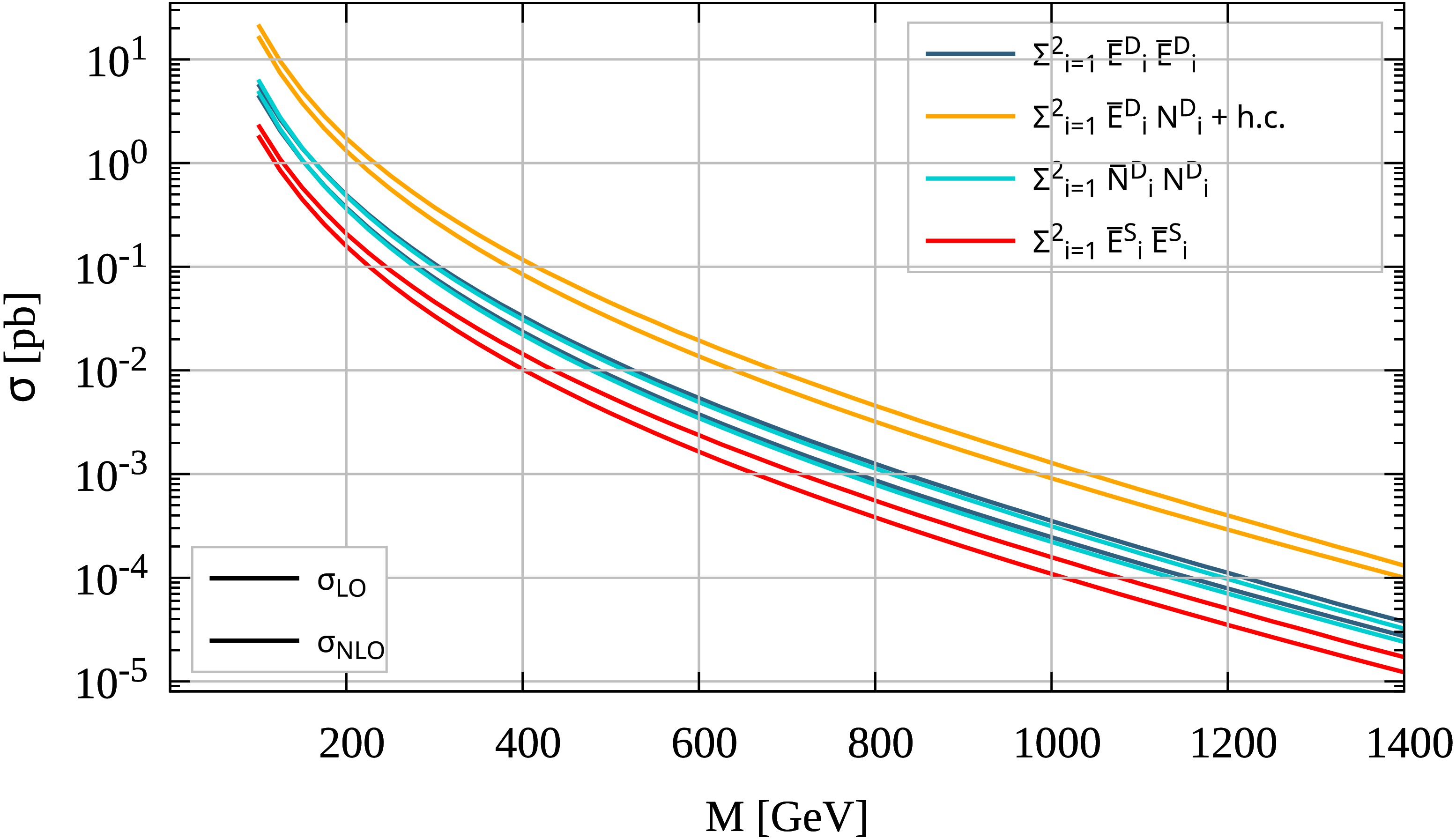
Figure 7. (color online) Cross-section (in pb) for the production of
$ Z_2 $ -odd leptons at the 13 TeV LHC. In the limit of zero singlet-doublet mixing, the particles produced in each pair are mass-degenerate and thus, the mass on the x-axis corresponds to the physical mass of the particles produced in each pair. -
The gauge interactions of the exotic leptons and scalars facilitate the pair and associated production of the
$ Z_2 $ -odd exotics at the LHC through Drell-Yan processes (i.e., s-channel$ W^\pm/Z/\gamma $ mediation)23 . The production cross-sections are computed at the leading order (LO) and next-to-leading order (NLO) in${\mathrm{MG5}\_\mathrm{aMC}\_\mathrm{v2.9.9}}$ using${\mathrm{NN23LO1}}$ as the parton distribution function, with the renormalization and factorization scales set at$ m_Z $ . The NLO computation of the cross-section has been performed using the Universal$ \text{F}{\small{\text{EYN}}}\text{R}{\small{\text{ULES}}} $ Output (UFO) model [132]. We find that the LO and NLO K-factors vary between$ 1.28-1.46 $ as a function of the exotic lepton mass. Fig. 7 demonstrates the LO and NLO production cross-sections24 of the exotic leptons plotted against their masses. In the limit of zero singlet-doublet mixing, the particle spectrum simply corresponds to$ E^D_i = E^D_{L,i} + E^D_{R,i} $ ,$ E^S_i = E^S_{L,i} + E^S_{R,i} $ , and$ N^D_i = N^D_{L,i} + N^D_{R,i} $ where$ i = 1, 2 $ . Further, as gauge bosons couple only to gauge states of the same generation, the production of a pair of doublets (singlets) of two different generations will not occur. The pair-production cross-sections for these exotic leptons vary from a few picobarns to a fraction of a femtobarn as we vary their masses from 100 GeV to a TeV. Hence, a substantial quantity of the exotic leptons is anticipated to be produced at the LHC, offering a potential avenue for testing the model in collider experiments. The nature of final state signatures, though, depends crucially on how these exotics decay, which we discuss next.
Figure 7. (color online) Cross-section (in pb) for the production of
$ Z_2 $ -odd leptons at the 13 TeV LHC. In the limit of zero singlet-doublet mixing, the particles produced in each pair are mass-degenerate and thus, the mass on the x-axis corresponds to the physical mass of the particles produced in each pair. -
The gauge interactions of the exotic leptons and scalars facilitate the pair and associated production of the
$ Z_2 $ -odd exotics at the LHC through Drell-Yan processes (i.e., s-channel$ W^\pm/Z/\gamma $ mediation)23 . The production cross-sections are computed at the leading order (LO) and next-to-leading order (NLO) in${\mathrm{MG5}\_\mathrm{aMC}\_\mathrm{v2.9.9}}$ using${\mathrm{NN23LO1}}$ as the parton distribution function, with the renormalization and factorization scales set at$ m_Z $ . The NLO computation of the cross-section has been performed using the Universal$ \text{F}{\small{\text{EYN}}}\text{R}{\small{\text{ULES}}} $ Output (UFO) model [132]. We find that the LO and NLO K-factors vary between$ 1.28-1.46 $ as a function of the exotic lepton mass. Fig. 7 demonstrates the LO and NLO production cross-sections24 of the exotic leptons plotted against their masses. In the limit of zero singlet-doublet mixing, the particle spectrum simply corresponds to$ E^D_i = E^D_{L,i} + E^D_{R,i} $ ,$ E^S_i = E^S_{L,i} + E^S_{R,i} $ , and$ N^D_i = N^D_{L,i} + N^D_{R,i} $ where$ i = 1, 2 $ . Further, as gauge bosons couple only to gauge states of the same generation, the production of a pair of doublets (singlets) of two different generations will not occur. The pair-production cross-sections for these exotic leptons vary from a few picobarns to a fraction of a femtobarn as we vary their masses from 100 GeV to a TeV. Hence, a substantial quantity of the exotic leptons is anticipated to be produced at the LHC, offering a potential avenue for testing the model in collider experiments. The nature of final state signatures, though, depends crucially on how these exotics decay, which we discuss next.
Figure 7. (color online) Cross-section (in pb) for the production of
$ Z_2 $ -odd leptons at the 13 TeV LHC. In the limit of zero singlet-doublet mixing, the particles produced in each pair are mass-degenerate and thus, the mass on the x-axis corresponds to the physical mass of the particles produced in each pair. -
The gauge interactions of the exotic leptons and scalars facilitate the pair and associated production of the
$ Z_2 $ -odd exotics at the LHC through Drell-Yan processes (i.e., s-channel$ W^\pm/Z/\gamma $ mediation)23 . The production cross-sections are computed at the leading order (LO) and next-to-leading order (NLO) in${\mathrm{MG5}\_\mathrm{aMC}\_\mathrm{v2.9.9}}$ using${\mathrm{NN23LO1}}$ as the parton distribution function, with the renormalization and factorization scales set at$ m_Z $ . The NLO computation of the cross-section has been performed using the Universal$ \text{F}{\small{\text{EYN}}}\text{R}{\small{\text{ULES}}} $ Output (UFO) model [132]. We find that the LO and NLO K-factors vary between$ 1.28-1.46 $ as a function of the exotic lepton mass. Fig. 7 demonstrates the LO and NLO production cross-sections24 of the exotic leptons plotted against their masses. In the limit of zero singlet-doublet mixing, the particle spectrum simply corresponds to$ E^D_i = E^D_{L,i} + E^D_{R,i} $ ,$ E^S_i = E^S_{L,i} + E^S_{R,i} $ , and$ N^D_i = N^D_{L,i} + N^D_{R,i} $ where$ i = 1, 2 $ . Further, as gauge bosons couple only to gauge states of the same generation, the production of a pair of doublets (singlets) of two different generations will not occur. The pair-production cross-sections for these exotic leptons vary from a few picobarns to a fraction of a femtobarn as we vary their masses from 100 GeV to a TeV. Hence, a substantial quantity of the exotic leptons is anticipated to be produced at the LHC, offering a potential avenue for testing the model in collider experiments. The nature of final state signatures, though, depends crucially on how these exotics decay, which we discuss next.
Figure 7. (color online) Cross-section (in pb) for the production of
$ Z_2 $ -odd leptons at the 13 TeV LHC. In the limit of zero singlet-doublet mixing, the particles produced in each pair are mass-degenerate and thus, the mass on the x-axis corresponds to the physical mass of the particles produced in each pair. -
The gauge interactions of the exotic leptons and scalars facilitate the pair and associated production of the
$ Z_2 $ -odd exotics at the LHC through Drell-Yan processes (i.e., s-channel$ W^\pm/Z/\gamma $ mediation)23 . The production cross-sections are computed at the leading order (LO) and next-to-leading order (NLO) in${\mathrm{MG5}\_\mathrm{aMC}\_\mathrm{v2.9.9}}$ using${\mathrm{NN23LO1}}$ as the parton distribution function, with the renormalization and factorization scales set at$ m_Z $ . The NLO computation of the cross-section has been performed using the Universal$ \text{F}{\small{\text{EYN}}}\text{R}{\small{\text{ULES}}} $ Output (UFO) model [132]. We find that the LO and NLO K-factors vary between$ 1.28-1.46 $ as a function of the exotic lepton mass. Fig. 7 demonstrates the LO and NLO production cross-sections24 of the exotic leptons plotted against their masses. In the limit of zero singlet-doublet mixing, the particle spectrum simply corresponds to$ E^D_i = E^D_{L,i} + E^D_{R,i} $ ,$ E^S_i = E^S_{L,i} + E^S_{R,i} $ , and$ N^D_i = N^D_{L,i} + N^D_{R,i} $ where$ i = 1, 2 $ . Further, as gauge bosons couple only to gauge states of the same generation, the production of a pair of doublets (singlets) of two different generations will not occur. The pair-production cross-sections for these exotic leptons vary from a few picobarns to a fraction of a femtobarn as we vary their masses from 100 GeV to a TeV. Hence, a substantial quantity of the exotic leptons is anticipated to be produced at the LHC, offering a potential avenue for testing the model in collider experiments. The nature of final state signatures, though, depends crucially on how these exotics decay, which we discuss next.
Figure 7. (color online) Cross-section (in pb) for the production of
$ Z_2 $ -odd leptons at the 13 TeV LHC. In the limit of zero singlet-doublet mixing, the particles produced in each pair are mass-degenerate and thus, the mass on the x-axis corresponds to the physical mass of the particles produced in each pair. -
The gauge interactions of the exotic leptons and scalars facilitate the pair and associated production of the
$ Z_2 $ -odd exotics at the LHC through Drell-Yan processes (i.e., s-channel$ W^\pm/Z/\gamma $ mediation)23 . The production cross-sections are computed at the leading order (LO) and next-to-leading order (NLO) in${\mathrm{MG5}\_\mathrm{aMC}\_\mathrm{v2.9.9}}$ using${\mathrm{NN23LO1}}$ as the parton distribution function, with the renormalization and factorization scales set at$ m_Z $ . The NLO computation of the cross-section has been performed using the Universal$ \text{F}{\small{\text{EYN}}}\text{R}{\small{\text{ULES}}} $ Output (UFO) model [132]. We find that the LO and NLO K-factors vary between$ 1.28-1.46 $ as a function of the exotic lepton mass. Fig. 7 demonstrates the LO and NLO production cross-sections24 of the exotic leptons plotted against their masses. In the limit of zero singlet-doublet mixing, the particle spectrum simply corresponds to$ E^D_i = E^D_{L,i} + E^D_{R,i} $ ,$ E^S_i = E^S_{L,i} + E^S_{R,i} $ , and$ N^D_i = N^D_{L,i} + N^D_{R,i} $ where$ i = 1, 2 $ . Further, as gauge bosons couple only to gauge states of the same generation, the production of a pair of doublets (singlets) of two different generations will not occur. The pair-production cross-sections for these exotic leptons vary from a few picobarns to a fraction of a femtobarn as we vary their masses from 100 GeV to a TeV. Hence, a substantial quantity of the exotic leptons is anticipated to be produced at the LHC, offering a potential avenue for testing the model in collider experiments. The nature of final state signatures, though, depends crucially on how these exotics decay, which we discuss next.
Figure 7. (color online) Cross-section (in pb) for the production of
$ Z_2 $ -odd leptons at the 13 TeV LHC. In the limit of zero singlet-doublet mixing, the particles produced in each pair are mass-degenerate and thus, the mass on the x-axis corresponds to the physical mass of the particles produced in each pair. -
The gauge interactions of the exotic leptons and scalars facilitate the pair and associated production of the
$ Z_2 $ -odd exotics at the LHC through Drell-Yan processes (i.e., s-channel$ W^\pm/Z/\gamma $ mediation)23 . The production cross-sections are computed at the leading order (LO) and next-to-leading order (NLO) in${\mathrm{MG5}\_\mathrm{aMC}\_\mathrm{v2.9.9}}$ using${\mathrm{NN23LO1}}$ as the parton distribution function, with the renormalization and factorization scales set at$ m_Z $ . The NLO computation of the cross-section has been performed using the Universal$ \text{F}{\small{\text{EYN}}}\text{R}{\small{\text{ULES}}} $ Output (UFO) model [132]. We find that the LO and NLO K-factors vary between$ 1.28-1.46 $ as a function of the exotic lepton mass. Fig. 7 demonstrates the LO and NLO production cross-sections24 of the exotic leptons plotted against their masses. In the limit of zero singlet-doublet mixing, the particle spectrum simply corresponds to$ E^D_i = E^D_{L,i} + E^D_{R,i} $ ,$ E^S_i = E^S_{L,i} + E^S_{R,i} $ , and$ N^D_i = N^D_{L,i} + N^D_{R,i} $ where$ i = 1, 2 $ . Further, as gauge bosons couple only to gauge states of the same generation, the production of a pair of doublets (singlets) of two different generations will not occur. The pair-production cross-sections for these exotic leptons vary from a few picobarns to a fraction of a femtobarn as we vary their masses from 100 GeV to a TeV. Hence, a substantial quantity of the exotic leptons is anticipated to be produced at the LHC, offering a potential avenue for testing the model in collider experiments. The nature of final state signatures, though, depends crucially on how these exotics decay, which we discuss next.
Figure 7. (color online) Cross-section (in pb) for the production of
$ Z_2 $ -odd leptons at the 13 TeV LHC. In the limit of zero singlet-doublet mixing, the particles produced in each pair are mass-degenerate and thus, the mass on the x-axis corresponds to the physical mass of the particles produced in each pair. -
The pair-produced
$ Z_2 $ -odd exotics at the LHC each decay into a lighter$ Z_2 $ -odd particle and an on-shell or off-shell25 SM particle. The decays proceed via the gauge couplings or Yukawa couplings (involving the SM Higgs or$ Z_2 $ -odd scalars). The daughter$ Z_2 $ -odd particle will decay further until the lightest$ Z_2 $ -odd particle is produced. This results in a decay cascade for a given exotic particle, as shown in Fig. 8 (top) and Fig. 8 (bottom), respectively, for the two distinct mass hierarchies as defined in Tables 2 and 3. The parameters$ \widetilde m_N $ and$ d_2 $ ($ z_{{LN}} $ ), however, are chosen from the feasible space in Fig. 6. Hereafter, we use the notation$ { \widetilde N^D}_{\gamma} $ with$ \gamma=1-4 $ to denote the doublet eigenstates$ { \widetilde N^D}_{X, \kappa} $ and$ { \widetilde N^D}_{Y,\kappa} $ with$ \kappa=1,2 $ .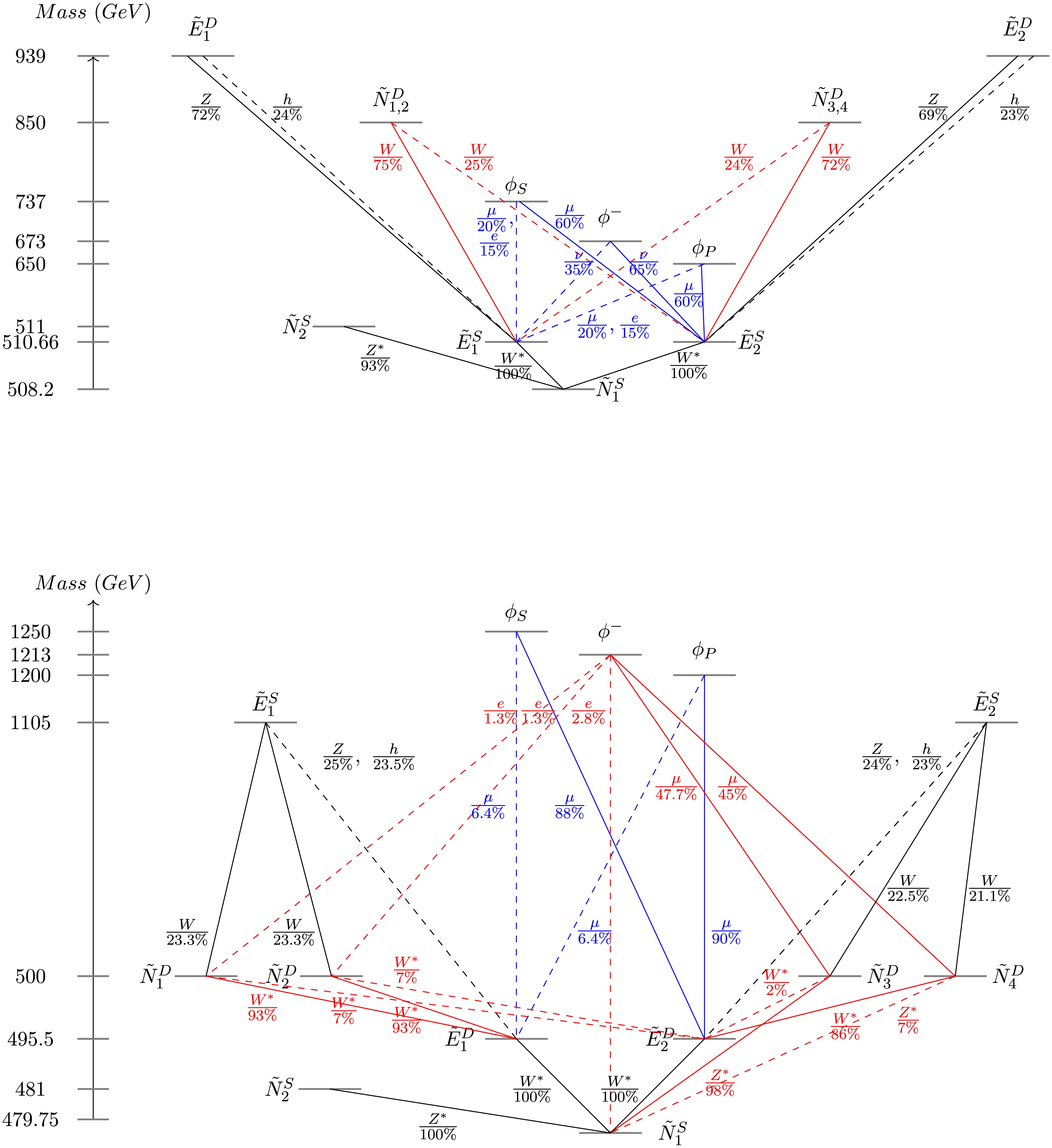
Figure 8. (color online) Decay Cascades at MH1 (
$ \widetilde m_N \lt \widetilde m_E \lt $ $ \mu_{\Phi} \lt \widetilde m_L $ ) (top) and MH2 ($ \widetilde m_N \lt \widetilde m_L \lt \widetilde m_E \lt \mu_{\Phi} $ ) (bottom). The quoted percentages indicate the corresponding branching ratios and include the conjugate process wherever allowed. Different colors are used only for better readability and do not follow any particular color scheme. Only dominant (solid lines) and subdominant (dashed lines) decay modes are shown.Scenario I (Mass hierarchy 1 in Table 2): The decay cascades for this scenario are illustrated in Fig. 8 (top). The Yukawa couplings and mass parameters for Mass hierarchy 1 (MH1) yield a mass spectrum of the
$ Z_2 $ -odd particles where the exotic doublet leptons are heavier than the singlets, with the charged component of the$ Z_2 $ -odd doublet being the heaviest of them all.1. While the decays of the charged exotic doublet leptons (
$ { \widetilde E^D}_{1,2} $ ) into the neutral components of$ Z_2 $ -odd doublets ($ { \widetilde N^D}_{X,Y} $ ) are kinematically suppressed, the decays into$ Z_2 $ -odd scalars ($ \phi_{S,P} $ ) are suppressed by the smallness of the Yukawa coupling,$ y_{{eL}} $ . Therefore,$ { \widetilde E^D}_{1,2} $ predominantly decay into singlet$ Z_2 $ -odd charged leptons ($ { \widetilde E^S}_{1,2} $ ) in association with a Z or Higgs boson. The decays are assisted by the considerable magnitude of the Yukawa coupling,$ z_{{RE}} $ , introducing a significant mixing between the charged components of the$ Z_2 $ -odd singlets and doublets.2. The neutral doublet
$ Z_2 $ -odd leptons ($ { \widetilde N^D}_{1-4} $ ), being lighter than$ { \widetilde E^D}_{1,2} $ , cannot decay into$ { \widetilde E^D}_{1,2} $ . They predominantly decay into the singlet$ Z_2 $ -odd charged leptons ($ { \widetilde E^S}_{1,2} $ ) along with a$ W^\pm $ boson, exhibiting an almost 100% branching ratio for this decay channel. It should be noted that this decay is possible because of the large mixing ($ z_{{RE}} $ ) between$ \widetilde E^D $ and$ \widetilde E^S $ . Decays into charged$ Z_2 $ -odd scalars are suppressed by the small Yukawa coupling,$ y_{{eL}} $ , while decays into neutral$ Z_2 $ -odd scalars are not possible as there is no coupling involving the$ Z_2 $ -odd doublet and the SM ν. Furthermore, decays into$ N^S_R $ are also suppressed because of the tiny$ z_{{LN}} $ , despite the phase space being large.3. The neutral (
$ \phi_{S,P} $ ) and charged ($ \phi^{\pm} $ ) exotic scalars may decay into exotic charged singlets. Decays into$ { \widetilde N^S}_{1,2} $ are highly suppressed as the ratio$ y_{_{lN}} / y_{{lE}} \sim{\cal{O}}(10^{-2}) $ .4. For
$ { \widetilde E^S}_{1,2} $ , the only kinematically allowed decay modes are into$ { \widetilde N^S}_{1} $ and an off-shell$ W^{\pm} $ . In addition to being a 3-body decay with a relatively small phase space, this process is also severely suppressed by the singlet-doublet mixing.5. Similarly, the exotic neutral (
$ { \widetilde N^S}_2 $ ) decays into the lightest one ($ { \widetilde N^S}_1 $ ) and an SM fermion-antifermion pair via an off-shell Z-boson. The mixing suppression is even more pronounced in this case.Scenario II (Mass hierarchy 2 in Table 3): The decay cascades for this scenario are illustrated in Fig. 8 (bottom). This particular scenario is characterized by a mass spectrum where the scalars (
$ \phi_{S,P},\; \phi^\pm $ ) are the heaviest among the exotics, followed by the singlet charged leptons ($ { \widetilde E^S}_{1,2} $ ), doublet neutral leptons ($ { \widetilde N^D}_{1-4} $ ), doublet charged leptons ($ { \widetilde E^D}_{1,2} $ ), and singlet neutral leptons ($ { \widetilde N^S}_{1,2} $ ), in that order. Given this spectrum, the relic density of dark matter ($ { \widetilde N^S}_1 $ ) is satisfied through co-annihilations involving the nearly degenerate$ { \widetilde E^D}_{1,2} $ . This is in contrast to Scenario I where dark matter relic density is satisfied through co-annihilations involving$ { \widetilde E^S}_{1,2} $ . The various decays are described below.1. The
$ Z_2 $ -odd scalars can decay into singlet and doublet exotic leptons in association with an SM lepton. The neutral exotic scalars ($ \phi_{S,P} $ ) predominantly decay into$ { \widetilde E^D}_{2} $ in association with an electron or a muon, with the decay into muons dominating due to the specific structure of the Yukawa coupling$ y_{{eL}} $ (refer to Tables 2 and 3), which is necessary to obtain the correct anomalous magnetic moments of the electron and muon. For the same reason, the charged exotic scalar ($ \phi^\pm $ ) predominantly decays into$ { \widetilde N^D}_{3,4} $ , accompanied by muons. Decays into singlet charged leptons ($ { \widetilde E^S}_{1,2} $ ) are kinematically suppressed, while decays into singlet neutral leptons ($ { \widetilde N^S}_{1,2} $ ), although suppressed by the smallness of$ y_{lN} $ , are still present.2. The singlets
$ { \widetilde E^S}_{1,2} $ decay into the doublets$ { \widetilde E^D}_{1,2} $ and$ { \widetilde N^D}_{1-4} $ in association with a Z/Higgs boson and a$ W^\pm $ boson, respectively. These decays are made possible by virtue of the singlet-doublet mixing induced by the Yukawa coupling,$ z_{{RE}} $ .3. The only kinematically allowed decay modes for the neutral doublet leptons,
$ { \widetilde N^D}_{1-4} $ , are into either$ { \widetilde E^D}_{1,2} $ or$ { \widetilde N^S}_{1,2} $ . The decays into$ { \widetilde E^D}_{1,2} $ occur via off-shell$ W^{\pm} $ bosons, while decays into$ { \widetilde N^S}_{1,2} $ occur via off-shell$ Z/h $ bosons26 . Both decays depend on the relative magnitudes of the singlet-doublet components in$ \widetilde N^D $ ,$ \widetilde E^D $ , and$ \widetilde N^S $ and, therefore, the Yukawa couplings$ z_{{LN}} $ and$ z_{{RE}} $ .4. The doublet charged leptons (
$ { \widetilde E^D}_{1,2} $ ), being the next-to-lightest$ Z_2 $ -odd particles27 , can only decay into the lightest$ Z_2 $ -odd particles ($ { \widetilde N^S}_{1,2} $ ) in association with an SM fermion-antifermion pair. These decays are tree-level 3-body processes that proceed through a$ W^\pm $ boson in the propagator. -
The pair-produced
$ Z_2 $ -odd exotics at the LHC each decay into a lighter$ Z_2 $ -odd particle and an on-shell or off-shell25 SM particle. The decays proceed via the gauge couplings or Yukawa couplings (involving the SM Higgs or$ Z_2 $ -odd scalars). The daughter$ Z_2 $ -odd particle will decay further until the lightest$ Z_2 $ -odd particle is produced. This results in a decay cascade for a given exotic particle, as shown in Fig. 8 (top) and Fig. 8 (bottom), respectively, for the two distinct mass hierarchies as defined in Tables 2 and 3. The parameters$ \widetilde m_N $ and$ d_2 $ ($ z_{{LN}} $ ), however, are chosen from the feasible space in Fig. 6. Hereafter, we use the notation$ { \widetilde N^D}_{\gamma} $ with$ \gamma=1-4 $ to denote the doublet eigenstates$ { \widetilde N^D}_{X, \kappa} $ and$ { \widetilde N^D}_{Y,\kappa} $ with$ \kappa=1,2 $ .
Figure 8. (color online) Decay Cascades at MH1 (
$ \widetilde m_N \lt \widetilde m_E \lt $ $ \mu_{\Phi} \lt \widetilde m_L $ ) (top) and MH2 ($ \widetilde m_N \lt \widetilde m_L \lt \widetilde m_E \lt \mu_{\Phi} $ ) (bottom). The quoted percentages indicate the corresponding branching ratios and include the conjugate process wherever allowed. Different colors are used only for better readability and do not follow any particular color scheme. Only dominant (solid lines) and subdominant (dashed lines) decay modes are shown.Scenario I (Mass hierarchy 1 in Table 2): The decay cascades for this scenario are illustrated in Fig. 8 (top). The Yukawa couplings and mass parameters for Mass hierarchy 1 (MH1) yield a mass spectrum of the
$ Z_2 $ -odd particles where the exotic doublet leptons are heavier than the singlets, with the charged component of the$ Z_2 $ -odd doublet being the heaviest of them all.1. While the decays of the charged exotic doublet leptons (
$ { \widetilde E^D}_{1,2} $ ) into the neutral components of$ Z_2 $ -odd doublets ($ { \widetilde N^D}_{X,Y} $ ) are kinematically suppressed, the decays into$ Z_2 $ -odd scalars ($ \phi_{S,P} $ ) are suppressed by the smallness of the Yukawa coupling,$ y_{{eL}} $ . Therefore,$ { \widetilde E^D}_{1,2} $ predominantly decay into singlet$ Z_2 $ -odd charged leptons ($ { \widetilde E^S}_{1,2} $ ) in association with a Z or Higgs boson. The decays are assisted by the considerable magnitude of the Yukawa coupling,$ z_{{RE}} $ , introducing a significant mixing between the charged components of the$ Z_2 $ -odd singlets and doublets.2. The neutral doublet
$ Z_2 $ -odd leptons ($ { \widetilde N^D}_{1-4} $ ), being lighter than$ { \widetilde E^D}_{1,2} $ , cannot decay into$ { \widetilde E^D}_{1,2} $ . They predominantly decay into the singlet$ Z_2 $ -odd charged leptons ($ { \widetilde E^S}_{1,2} $ ) along with a$ W^\pm $ boson, exhibiting an almost 100% branching ratio for this decay channel. It should be noted that this decay is possible because of the large mixing ($ z_{{RE}} $ ) between$ \widetilde E^D $ and$ \widetilde E^S $ . Decays into charged$ Z_2 $ -odd scalars are suppressed by the small Yukawa coupling,$ y_{{eL}} $ , while decays into neutral$ Z_2 $ -odd scalars are not possible as there is no coupling involving the$ Z_2 $ -odd doublet and the SM ν. Furthermore, decays into$ N^S_R $ are also suppressed because of the tiny$ z_{{LN}} $ , despite the phase space being large.3. The neutral (
$ \phi_{S,P} $ ) and charged ($ \phi^{\pm} $ ) exotic scalars may decay into exotic charged singlets. Decays into$ { \widetilde N^S}_{1,2} $ are highly suppressed as the ratio$ y_{_{lN}} / y_{{lE}} \sim{\cal{O}}(10^{-2}) $ .4. For
$ { \widetilde E^S}_{1,2} $ , the only kinematically allowed decay modes are into$ { \widetilde N^S}_{1} $ and an off-shell$ W^{\pm} $ . In addition to being a 3-body decay with a relatively small phase space, this process is also severely suppressed by the singlet-doublet mixing.5. Similarly, the exotic neutral (
$ { \widetilde N^S}_2 $ ) decays into the lightest one ($ { \widetilde N^S}_1 $ ) and an SM fermion-antifermion pair via an off-shell Z-boson. The mixing suppression is even more pronounced in this case.Scenario II (Mass hierarchy 2 in Table 3): The decay cascades for this scenario are illustrated in Fig. 8 (bottom). This particular scenario is characterized by a mass spectrum where the scalars (
$ \phi_{S,P},\; \phi^\pm $ ) are the heaviest among the exotics, followed by the singlet charged leptons ($ { \widetilde E^S}_{1,2} $ ), doublet neutral leptons ($ { \widetilde N^D}_{1-4} $ ), doublet charged leptons ($ { \widetilde E^D}_{1,2} $ ), and singlet neutral leptons ($ { \widetilde N^S}_{1,2} $ ), in that order. Given this spectrum, the relic density of dark matter ($ { \widetilde N^S}_1 $ ) is satisfied through co-annihilations involving the nearly degenerate$ { \widetilde E^D}_{1,2} $ . This is in contrast to Scenario I where dark matter relic density is satisfied through co-annihilations involving$ { \widetilde E^S}_{1,2} $ . The various decays are described below.1. The
$ Z_2 $ -odd scalars can decay into singlet and doublet exotic leptons in association with an SM lepton. The neutral exotic scalars ($ \phi_{S,P} $ ) predominantly decay into$ { \widetilde E^D}_{2} $ in association with an electron or a muon, with the decay into muons dominating due to the specific structure of the Yukawa coupling$ y_{{eL}} $ (refer to Tables 2 and 3), which is necessary to obtain the correct anomalous magnetic moments of the electron and muon. For the same reason, the charged exotic scalar ($ \phi^\pm $ ) predominantly decays into$ { \widetilde N^D}_{3,4} $ , accompanied by muons. Decays into singlet charged leptons ($ { \widetilde E^S}_{1,2} $ ) are kinematically suppressed, while decays into singlet neutral leptons ($ { \widetilde N^S}_{1,2} $ ), although suppressed by the smallness of$ y_{lN} $ , are still present.2. The singlets
$ { \widetilde E^S}_{1,2} $ decay into the doublets$ { \widetilde E^D}_{1,2} $ and$ { \widetilde N^D}_{1-4} $ in association with a Z/Higgs boson and a$ W^\pm $ boson, respectively. These decays are made possible by virtue of the singlet-doublet mixing induced by the Yukawa coupling,$ z_{{RE}} $ .3. The only kinematically allowed decay modes for the neutral doublet leptons,
$ { \widetilde N^D}_{1-4} $ , are into either$ { \widetilde E^D}_{1,2} $ or$ { \widetilde N^S}_{1,2} $ . The decays into$ { \widetilde E^D}_{1,2} $ occur via off-shell$ W^{\pm} $ bosons, while decays into$ { \widetilde N^S}_{1,2} $ occur via off-shell$ Z/h $ bosons26 . Both decays depend on the relative magnitudes of the singlet-doublet components in$ \widetilde N^D $ ,$ \widetilde E^D $ , and$ \widetilde N^S $ and, therefore, the Yukawa couplings$ z_{{LN}} $ and$ z_{{RE}} $ .4. The doublet charged leptons (
$ { \widetilde E^D}_{1,2} $ ), being the next-to-lightest$ Z_2 $ -odd particles27 , can only decay into the lightest$ Z_2 $ -odd particles ($ { \widetilde N^S}_{1,2} $ ) in association with an SM fermion-antifermion pair. These decays are tree-level 3-body processes that proceed through a$ W^\pm $ boson in the propagator. -
The pair-produced
$ Z_2 $ -odd exotics at the LHC each decay into a lighter$ Z_2 $ -odd particle and an on-shell or off-shell25 SM particle. The decays proceed via the gauge couplings or Yukawa couplings (involving the SM Higgs or$ Z_2 $ -odd scalars). The daughter$ Z_2 $ -odd particle will decay further until the lightest$ Z_2 $ -odd particle is produced. This results in a decay cascade for a given exotic particle, as shown in Fig. 8 (top) and Fig. 8 (bottom), respectively, for the two distinct mass hierarchies as defined in Tables 2 and 3. The parameters$ \widetilde m_N $ and$ d_2 $ ($ z_{{LN}} $ ), however, are chosen from the feasible space in Fig. 6. Hereafter, we use the notation$ { \widetilde N^D}_{\gamma} $ with$ \gamma=1-4 $ to denote the doublet eigenstates$ { \widetilde N^D}_{X, \kappa} $ and$ { \widetilde N^D}_{Y,\kappa} $ with$ \kappa=1,2 $ .
Figure 8. (color online) Decay Cascades at MH1 (
$ \widetilde m_N \lt \widetilde m_E \lt $ $ \mu_{\Phi} \lt \widetilde m_L $ ) (top) and MH2 ($ \widetilde m_N \lt \widetilde m_L \lt \widetilde m_E \lt \mu_{\Phi} $ ) (bottom). The quoted percentages indicate the corresponding branching ratios and include the conjugate process wherever allowed. Different colors are used only for better readability and do not follow any particular color scheme. Only dominant (solid lines) and subdominant (dashed lines) decay modes are shown.Scenario I (Mass hierarchy 1 in Table 2): The decay cascades for this scenario are illustrated in Fig. 8 (top). The Yukawa couplings and mass parameters for Mass hierarchy 1 (MH1) yield a mass spectrum of the
$ Z_2 $ -odd particles where the exotic doublet leptons are heavier than the singlets, with the charged component of the$ Z_2 $ -odd doublet being the heaviest of them all.1. While the decays of the charged exotic doublet leptons (
$ { \widetilde E^D}_{1,2} $ ) into the neutral components of$ Z_2 $ -odd doublets ($ { \widetilde N^D}_{X,Y} $ ) are kinematically suppressed, the decays into$ Z_2 $ -odd scalars ($ \phi_{S,P} $ ) are suppressed by the smallness of the Yukawa coupling,$ y_{{eL}} $ . Therefore,$ { \widetilde E^D}_{1,2} $ predominantly decay into singlet$ Z_2 $ -odd charged leptons ($ { \widetilde E^S}_{1,2} $ ) in association with a Z or Higgs boson. The decays are assisted by the considerable magnitude of the Yukawa coupling,$ z_{{RE}} $ , introducing a significant mixing between the charged components of the$ Z_2 $ -odd singlets and doublets.2. The neutral doublet
$ Z_2 $ -odd leptons ($ { \widetilde N^D}_{1-4} $ ), being lighter than$ { \widetilde E^D}_{1,2} $ , cannot decay into$ { \widetilde E^D}_{1,2} $ . They predominantly decay into the singlet$ Z_2 $ -odd charged leptons ($ { \widetilde E^S}_{1,2} $ ) along with a$ W^\pm $ boson, exhibiting an almost 100% branching ratio for this decay channel. It should be noted that this decay is possible because of the large mixing ($ z_{{RE}} $ ) between$ \widetilde E^D $ and$ \widetilde E^S $ . Decays into charged$ Z_2 $ -odd scalars are suppressed by the small Yukawa coupling,$ y_{{eL}} $ , while decays into neutral$ Z_2 $ -odd scalars are not possible as there is no coupling involving the$ Z_2 $ -odd doublet and the SM ν. Furthermore, decays into$ N^S_R $ are also suppressed because of the tiny$ z_{{LN}} $ , despite the phase space being large.3. The neutral (
$ \phi_{S,P} $ ) and charged ($ \phi^{\pm} $ ) exotic scalars may decay into exotic charged singlets. Decays into$ { \widetilde N^S}_{1,2} $ are highly suppressed as the ratio$ y_{_{lN}} / y_{{lE}} \sim{\cal{O}}(10^{-2}) $ .4. For
$ { \widetilde E^S}_{1,2} $ , the only kinematically allowed decay modes are into$ { \widetilde N^S}_{1} $ and an off-shell$ W^{\pm} $ . In addition to being a 3-body decay with a relatively small phase space, this process is also severely suppressed by the singlet-doublet mixing.5. Similarly, the exotic neutral (
$ { \widetilde N^S}_2 $ ) decays into the lightest one ($ { \widetilde N^S}_1 $ ) and an SM fermion-antifermion pair via an off-shell Z-boson. The mixing suppression is even more pronounced in this case.Scenario II (Mass hierarchy 2 in Table 3): The decay cascades for this scenario are illustrated in Fig. 8 (bottom). This particular scenario is characterized by a mass spectrum where the scalars (
$ \phi_{S,P},\; \phi^\pm $ ) are the heaviest among the exotics, followed by the singlet charged leptons ($ { \widetilde E^S}_{1,2} $ ), doublet neutral leptons ($ { \widetilde N^D}_{1-4} $ ), doublet charged leptons ($ { \widetilde E^D}_{1,2} $ ), and singlet neutral leptons ($ { \widetilde N^S}_{1,2} $ ), in that order. Given this spectrum, the relic density of dark matter ($ { \widetilde N^S}_1 $ ) is satisfied through co-annihilations involving the nearly degenerate$ { \widetilde E^D}_{1,2} $ . This is in contrast to Scenario I where dark matter relic density is satisfied through co-annihilations involving$ { \widetilde E^S}_{1,2} $ . The various decays are described below.1. The
$ Z_2 $ -odd scalars can decay into singlet and doublet exotic leptons in association with an SM lepton. The neutral exotic scalars ($ \phi_{S,P} $ ) predominantly decay into$ { \widetilde E^D}_{2} $ in association with an electron or a muon, with the decay into muons dominating due to the specific structure of the Yukawa coupling$ y_{{eL}} $ (refer to Tables 2 and 3), which is necessary to obtain the correct anomalous magnetic moments of the electron and muon. For the same reason, the charged exotic scalar ($ \phi^\pm $ ) predominantly decays into$ { \widetilde N^D}_{3,4} $ , accompanied by muons. Decays into singlet charged leptons ($ { \widetilde E^S}_{1,2} $ ) are kinematically suppressed, while decays into singlet neutral leptons ($ { \widetilde N^S}_{1,2} $ ), although suppressed by the smallness of$ y_{lN} $ , are still present.2. The singlets
$ { \widetilde E^S}_{1,2} $ decay into the doublets$ { \widetilde E^D}_{1,2} $ and$ { \widetilde N^D}_{1-4} $ in association with a Z/Higgs boson and a$ W^\pm $ boson, respectively. These decays are made possible by virtue of the singlet-doublet mixing induced by the Yukawa coupling,$ z_{{RE}} $ .3. The only kinematically allowed decay modes for the neutral doublet leptons,
$ { \widetilde N^D}_{1-4} $ , are into either$ { \widetilde E^D}_{1,2} $ or$ { \widetilde N^S}_{1,2} $ . The decays into$ { \widetilde E^D}_{1,2} $ occur via off-shell$ W^{\pm} $ bosons, while decays into$ { \widetilde N^S}_{1,2} $ occur via off-shell$ Z/h $ bosons26 . Both decays depend on the relative magnitudes of the singlet-doublet components in$ \widetilde N^D $ ,$ \widetilde E^D $ , and$ \widetilde N^S $ and, therefore, the Yukawa couplings$ z_{{LN}} $ and$ z_{{RE}} $ .4. The doublet charged leptons (
$ { \widetilde E^D}_{1,2} $ ), being the next-to-lightest$ Z_2 $ -odd particles27 , can only decay into the lightest$ Z_2 $ -odd particles ($ { \widetilde N^S}_{1,2} $ ) in association with an SM fermion-antifermion pair. These decays are tree-level 3-body processes that proceed through a$ W^\pm $ boson in the propagator. -
The pair-produced
$ Z_2 $ -odd exotics at the LHC each decay into a lighter$ Z_2 $ -odd particle and an on-shell or off-shell25 SM particle. The decays proceed via the gauge couplings or Yukawa couplings (involving the SM Higgs or$ Z_2 $ -odd scalars). The daughter$ Z_2 $ -odd particle will decay further until the lightest$ Z_2 $ -odd particle is produced. This results in a decay cascade for a given exotic particle, as shown in Fig. 8 (top) and Fig. 8 (bottom), respectively, for the two distinct mass hierarchies as defined in Tables 2 and 3. The parameters$ \widetilde m_N $ and$ d_2 $ ($ z_{{LN}} $ ), however, are chosen from the feasible space in Fig. 6. Hereafter, we use the notation$ { \widetilde N^D}_{\gamma} $ with$ \gamma=1-4 $ to denote the doublet eigenstates$ { \widetilde N^D}_{X, \kappa} $ and$ { \widetilde N^D}_{Y,\kappa} $ with$ \kappa=1,2 $ .
Figure 8. (color online) Decay Cascades at MH1 (
$ \widetilde m_N \lt \widetilde m_E \lt $ $ \mu_{\Phi} \lt \widetilde m_L $ ) (top) and MH2 ($ \widetilde m_N \lt \widetilde m_L \lt \widetilde m_E \lt \mu_{\Phi} $ ) (bottom). The quoted percentages indicate the corresponding branching ratios and include the conjugate process wherever allowed. Different colors are used only for better readability and do not follow any particular color scheme. Only dominant (solid lines) and subdominant (dashed lines) decay modes are shown.Scenario I (Mass hierarchy 1 in Table 2): The decay cascades for this scenario are illustrated in Fig. 8 (top). The Yukawa couplings and mass parameters for Mass hierarchy 1 (MH1) yield a mass spectrum of the
$ Z_2 $ -odd particles where the exotic doublet leptons are heavier than the singlets, with the charged component of the$ Z_2 $ -odd doublet being the heaviest of them all.1. While the decays of the charged exotic doublet leptons (
$ { \widetilde E^D}_{1,2} $ ) into the neutral components of$ Z_2 $ -odd doublets ($ { \widetilde N^D}_{X,Y} $ ) are kinematically suppressed, the decays into$ Z_2 $ -odd scalars ($ \phi_{S,P} $ ) are suppressed by the smallness of the Yukawa coupling,$ y_{{eL}} $ . Therefore,$ { \widetilde E^D}_{1,2} $ predominantly decay into singlet$ Z_2 $ -odd charged leptons ($ { \widetilde E^S}_{1,2} $ ) in association with a Z or Higgs boson. The decays are assisted by the considerable magnitude of the Yukawa coupling,$ z_{{RE}} $ , introducing a significant mixing between the charged components of the$ Z_2 $ -odd singlets and doublets.2. The neutral doublet
$ Z_2 $ -odd leptons ($ { \widetilde N^D}_{1-4} $ ), being lighter than$ { \widetilde E^D}_{1,2} $ , cannot decay into$ { \widetilde E^D}_{1,2} $ . They predominantly decay into the singlet$ Z_2 $ -odd charged leptons ($ { \widetilde E^S}_{1,2} $ ) along with a$ W^\pm $ boson, exhibiting an almost 100% branching ratio for this decay channel. It should be noted that this decay is possible because of the large mixing ($ z_{{RE}} $ ) between$ \widetilde E^D $ and$ \widetilde E^S $ . Decays into charged$ Z_2 $ -odd scalars are suppressed by the small Yukawa coupling,$ y_{{eL}} $ , while decays into neutral$ Z_2 $ -odd scalars are not possible as there is no coupling involving the$ Z_2 $ -odd doublet and the SM ν. Furthermore, decays into$ N^S_R $ are also suppressed because of the tiny$ z_{{LN}} $ , despite the phase space being large.3. The neutral (
$ \phi_{S,P} $ ) and charged ($ \phi^{\pm} $ ) exotic scalars may decay into exotic charged singlets. Decays into$ { \widetilde N^S}_{1,2} $ are highly suppressed as the ratio$ y_{_{lN}} / y_{{lE}} \sim{\cal{O}}(10^{-2}) $ .4. For
$ { \widetilde E^S}_{1,2} $ , the only kinematically allowed decay modes are into$ { \widetilde N^S}_{1} $ and an off-shell$ W^{\pm} $ . In addition to being a 3-body decay with a relatively small phase space, this process is also severely suppressed by the singlet-doublet mixing.5. Similarly, the exotic neutral (
$ { \widetilde N^S}_2 $ ) decays into the lightest one ($ { \widetilde N^S}_1 $ ) and an SM fermion-antifermion pair via an off-shell Z-boson. The mixing suppression is even more pronounced in this case.Scenario II (Mass hierarchy 2 in Table 3): The decay cascades for this scenario are illustrated in Fig. 8 (bottom). This particular scenario is characterized by a mass spectrum where the scalars (
$ \phi_{S,P},\; \phi^\pm $ ) are the heaviest among the exotics, followed by the singlet charged leptons ($ { \widetilde E^S}_{1,2} $ ), doublet neutral leptons ($ { \widetilde N^D}_{1-4} $ ), doublet charged leptons ($ { \widetilde E^D}_{1,2} $ ), and singlet neutral leptons ($ { \widetilde N^S}_{1,2} $ ), in that order. Given this spectrum, the relic density of dark matter ($ { \widetilde N^S}_1 $ ) is satisfied through co-annihilations involving the nearly degenerate$ { \widetilde E^D}_{1,2} $ . This is in contrast to Scenario I where dark matter relic density is satisfied through co-annihilations involving$ { \widetilde E^S}_{1,2} $ . The various decays are described below.1. The
$ Z_2 $ -odd scalars can decay into singlet and doublet exotic leptons in association with an SM lepton. The neutral exotic scalars ($ \phi_{S,P} $ ) predominantly decay into$ { \widetilde E^D}_{2} $ in association with an electron or a muon, with the decay into muons dominating due to the specific structure of the Yukawa coupling$ y_{{eL}} $ (refer to Tables 2 and 3), which is necessary to obtain the correct anomalous magnetic moments of the electron and muon. For the same reason, the charged exotic scalar ($ \phi^\pm $ ) predominantly decays into$ { \widetilde N^D}_{3,4} $ , accompanied by muons. Decays into singlet charged leptons ($ { \widetilde E^S}_{1,2} $ ) are kinematically suppressed, while decays into singlet neutral leptons ($ { \widetilde N^S}_{1,2} $ ), although suppressed by the smallness of$ y_{lN} $ , are still present.2. The singlets
$ { \widetilde E^S}_{1,2} $ decay into the doublets$ { \widetilde E^D}_{1,2} $ and$ { \widetilde N^D}_{1-4} $ in association with a Z/Higgs boson and a$ W^\pm $ boson, respectively. These decays are made possible by virtue of the singlet-doublet mixing induced by the Yukawa coupling,$ z_{{RE}} $ .3. The only kinematically allowed decay modes for the neutral doublet leptons,
$ { \widetilde N^D}_{1-4} $ , are into either$ { \widetilde E^D}_{1,2} $ or$ { \widetilde N^S}_{1,2} $ . The decays into$ { \widetilde E^D}_{1,2} $ occur via off-shell$ W^{\pm} $ bosons, while decays into$ { \widetilde N^S}_{1,2} $ occur via off-shell$ Z/h $ bosons26 . Both decays depend on the relative magnitudes of the singlet-doublet components in$ \widetilde N^D $ ,$ \widetilde E^D $ , and$ \widetilde N^S $ and, therefore, the Yukawa couplings$ z_{{LN}} $ and$ z_{{RE}} $ .4. The doublet charged leptons (
$ { \widetilde E^D}_{1,2} $ ), being the next-to-lightest$ Z_2 $ -odd particles27 , can only decay into the lightest$ Z_2 $ -odd particles ($ { \widetilde N^S}_{1,2} $ ) in association with an SM fermion-antifermion pair. These decays are tree-level 3-body processes that proceed through a$ W^\pm $ boson in the propagator. -
The pair-produced
$ Z_2 $ -odd exotics at the LHC each decay into a lighter$ Z_2 $ -odd particle and an on-shell or off-shell25 SM particle. The decays proceed via the gauge couplings or Yukawa couplings (involving the SM Higgs or$ Z_2 $ -odd scalars). The daughter$ Z_2 $ -odd particle will decay further until the lightest$ Z_2 $ -odd particle is produced. This results in a decay cascade for a given exotic particle, as shown in Fig. 8 (top) and Fig. 8 (bottom), respectively, for the two distinct mass hierarchies as defined in Tables 2 and 3. The parameters$ \widetilde m_N $ and$ d_2 $ ($ z_{{LN}} $ ), however, are chosen from the feasible space in Fig. 6. Hereafter, we use the notation$ { \widetilde N^D}_{\gamma} $ with$ \gamma=1-4 $ to denote the doublet eigenstates$ { \widetilde N^D}_{X, \kappa} $ and$ { \widetilde N^D}_{Y,\kappa} $ with$ \kappa=1,2 $ .
Figure 8. (color online) Decay Cascades at MH1 (
$ \widetilde m_N \lt \widetilde m_E \lt $ $ \mu_{\Phi} \lt \widetilde m_L $ ) (top) and MH2 ($ \widetilde m_N \lt \widetilde m_L \lt \widetilde m_E \lt \mu_{\Phi} $ ) (bottom). The quoted percentages indicate the corresponding branching ratios and include the conjugate process wherever allowed. Different colors are used only for better readability and do not follow any particular color scheme. Only dominant (solid lines) and subdominant (dashed lines) decay modes are shown.Scenario I (Mass hierarchy 1 in Table 2): The decay cascades for this scenario are illustrated in Fig. 8 (top). The Yukawa couplings and mass parameters for Mass hierarchy 1 (MH1) yield a mass spectrum of the
$ Z_2 $ -odd particles where the exotic doublet leptons are heavier than the singlets, with the charged component of the$ Z_2 $ -odd doublet being the heaviest of them all.1. While the decays of the charged exotic doublet leptons (
$ { \widetilde E^D}_{1,2} $ ) into the neutral components of$ Z_2 $ -odd doublets ($ { \widetilde N^D}_{X,Y} $ ) are kinematically suppressed, the decays into$ Z_2 $ -odd scalars ($ \phi_{S,P} $ ) are suppressed by the smallness of the Yukawa coupling,$ y_{{eL}} $ . Therefore,$ { \widetilde E^D}_{1,2} $ predominantly decay into singlet$ Z_2 $ -odd charged leptons ($ { \widetilde E^S}_{1,2} $ ) in association with a Z or Higgs boson. The decays are assisted by the considerable magnitude of the Yukawa coupling,$ z_{{RE}} $ , introducing a significant mixing between the charged components of the$ Z_2 $ -odd singlets and doublets.2. The neutral doublet
$ Z_2 $ -odd leptons ($ { \widetilde N^D}_{1-4} $ ), being lighter than$ { \widetilde E^D}_{1,2} $ , cannot decay into$ { \widetilde E^D}_{1,2} $ . They predominantly decay into the singlet$ Z_2 $ -odd charged leptons ($ { \widetilde E^S}_{1,2} $ ) along with a$ W^\pm $ boson, exhibiting an almost 100% branching ratio for this decay channel. It should be noted that this decay is possible because of the large mixing ($ z_{{RE}} $ ) between$ \widetilde E^D $ and$ \widetilde E^S $ . Decays into charged$ Z_2 $ -odd scalars are suppressed by the small Yukawa coupling,$ y_{{eL}} $ , while decays into neutral$ Z_2 $ -odd scalars are not possible as there is no coupling involving the$ Z_2 $ -odd doublet and the SM ν. Furthermore, decays into$ N^S_R $ are also suppressed because of the tiny$ z_{{LN}} $ , despite the phase space being large.3. The neutral (
$ \phi_{S,P} $ ) and charged ($ \phi^{\pm} $ ) exotic scalars may decay into exotic charged singlets. Decays into$ { \widetilde N^S}_{1,2} $ are highly suppressed as the ratio$ y_{_{lN}} / y_{{lE}} \sim{\cal{O}}(10^{-2}) $ .4. For
$ { \widetilde E^S}_{1,2} $ , the only kinematically allowed decay modes are into$ { \widetilde N^S}_{1} $ and an off-shell$ W^{\pm} $ . In addition to being a 3-body decay with a relatively small phase space, this process is also severely suppressed by the singlet-doublet mixing.5. Similarly, the exotic neutral (
$ { \widetilde N^S}_2 $ ) decays into the lightest one ($ { \widetilde N^S}_1 $ ) and an SM fermion-antifermion pair via an off-shell Z-boson. The mixing suppression is even more pronounced in this case.Scenario II (Mass hierarchy 2 in Table 3): The decay cascades for this scenario are illustrated in Fig. 8 (bottom). This particular scenario is characterized by a mass spectrum where the scalars (
$ \phi_{S,P},\; \phi^\pm $ ) are the heaviest among the exotics, followed by the singlet charged leptons ($ { \widetilde E^S}_{1,2} $ ), doublet neutral leptons ($ { \widetilde N^D}_{1-4} $ ), doublet charged leptons ($ { \widetilde E^D}_{1,2} $ ), and singlet neutral leptons ($ { \widetilde N^S}_{1,2} $ ), in that order. Given this spectrum, the relic density of dark matter ($ { \widetilde N^S}_1 $ ) is satisfied through co-annihilations involving the nearly degenerate$ { \widetilde E^D}_{1,2} $ . This is in contrast to Scenario I where dark matter relic density is satisfied through co-annihilations involving$ { \widetilde E^S}_{1,2} $ . The various decays are described below.1. The
$ Z_2 $ -odd scalars can decay into singlet and doublet exotic leptons in association with an SM lepton. The neutral exotic scalars ($ \phi_{S,P} $ ) predominantly decay into$ { \widetilde E^D}_{2} $ in association with an electron or a muon, with the decay into muons dominating due to the specific structure of the Yukawa coupling$ y_{{eL}} $ (refer to Tables 2 and 3), which is necessary to obtain the correct anomalous magnetic moments of the electron and muon. For the same reason, the charged exotic scalar ($ \phi^\pm $ ) predominantly decays into$ { \widetilde N^D}_{3,4} $ , accompanied by muons. Decays into singlet charged leptons ($ { \widetilde E^S}_{1,2} $ ) are kinematically suppressed, while decays into singlet neutral leptons ($ { \widetilde N^S}_{1,2} $ ), although suppressed by the smallness of$ y_{lN} $ , are still present.2. The singlets
$ { \widetilde E^S}_{1,2} $ decay into the doublets$ { \widetilde E^D}_{1,2} $ and$ { \widetilde N^D}_{1-4} $ in association with a Z/Higgs boson and a$ W^\pm $ boson, respectively. These decays are made possible by virtue of the singlet-doublet mixing induced by the Yukawa coupling,$ z_{{RE}} $ .3. The only kinematically allowed decay modes for the neutral doublet leptons,
$ { \widetilde N^D}_{1-4} $ , are into either$ { \widetilde E^D}_{1,2} $ or$ { \widetilde N^S}_{1,2} $ . The decays into$ { \widetilde E^D}_{1,2} $ occur via off-shell$ W^{\pm} $ bosons, while decays into$ { \widetilde N^S}_{1,2} $ occur via off-shell$ Z/h $ bosons26 . Both decays depend on the relative magnitudes of the singlet-doublet components in$ \widetilde N^D $ ,$ \widetilde E^D $ , and$ \widetilde N^S $ and, therefore, the Yukawa couplings$ z_{{LN}} $ and$ z_{{RE}} $ .4. The doublet charged leptons (
$ { \widetilde E^D}_{1,2} $ ), being the next-to-lightest$ Z_2 $ -odd particles27 , can only decay into the lightest$ Z_2 $ -odd particles ($ { \widetilde N^S}_{1,2} $ ) in association with an SM fermion-antifermion pair. These decays are tree-level 3-body processes that proceed through a$ W^\pm $ boson in the propagator. -
The pair-produced
$ Z_2 $ -odd exotics at the LHC each decay into a lighter$ Z_2 $ -odd particle and an on-shell or off-shell25 SM particle. The decays proceed via the gauge couplings or Yukawa couplings (involving the SM Higgs or$ Z_2 $ -odd scalars). The daughter$ Z_2 $ -odd particle will decay further until the lightest$ Z_2 $ -odd particle is produced. This results in a decay cascade for a given exotic particle, as shown in Fig. 8 (top) and Fig. 8 (bottom), respectively, for the two distinct mass hierarchies as defined in Tables 2 and 3. The parameters$ \widetilde m_N $ and$ d_2 $ ($ z_{{LN}} $ ), however, are chosen from the feasible space in Fig. 6. Hereafter, we use the notation$ { \widetilde N^D}_{\gamma} $ with$ \gamma=1-4 $ to denote the doublet eigenstates$ { \widetilde N^D}_{X, \kappa} $ and$ { \widetilde N^D}_{Y,\kappa} $ with$ \kappa=1,2 $ .
Figure 8. (color online) Decay Cascades at MH1 (
$ \widetilde m_N \lt \widetilde m_E \lt $ $ \mu_{\Phi} \lt \widetilde m_L $ ) (top) and MH2 ($ \widetilde m_N \lt \widetilde m_L \lt \widetilde m_E \lt \mu_{\Phi} $ ) (bottom). The quoted percentages indicate the corresponding branching ratios and include the conjugate process wherever allowed. Different colors are used only for better readability and do not follow any particular color scheme. Only dominant (solid lines) and subdominant (dashed lines) decay modes are shown.Scenario I (Mass hierarchy 1 in Table 2): The decay cascades for this scenario are illustrated in Fig. 8 (top). The Yukawa couplings and mass parameters for Mass hierarchy 1 (MH1) yield a mass spectrum of the
$ Z_2 $ -odd particles where the exotic doublet leptons are heavier than the singlets, with the charged component of the$ Z_2 $ -odd doublet being the heaviest of them all.1. While the decays of the charged exotic doublet leptons (
$ { \widetilde E^D}_{1,2} $ ) into the neutral components of$ Z_2 $ -odd doublets ($ { \widetilde N^D}_{X,Y} $ ) are kinematically suppressed, the decays into$ Z_2 $ -odd scalars ($ \phi_{S,P} $ ) are suppressed by the smallness of the Yukawa coupling,$ y_{{eL}} $ . Therefore,$ { \widetilde E^D}_{1,2} $ predominantly decay into singlet$ Z_2 $ -odd charged leptons ($ { \widetilde E^S}_{1,2} $ ) in association with a Z or Higgs boson. The decays are assisted by the considerable magnitude of the Yukawa coupling,$ z_{{RE}} $ , introducing a significant mixing between the charged components of the$ Z_2 $ -odd singlets and doublets.2. The neutral doublet
$ Z_2 $ -odd leptons ($ { \widetilde N^D}_{1-4} $ ), being lighter than$ { \widetilde E^D}_{1,2} $ , cannot decay into$ { \widetilde E^D}_{1,2} $ . They predominantly decay into the singlet$ Z_2 $ -odd charged leptons ($ { \widetilde E^S}_{1,2} $ ) along with a$ W^\pm $ boson, exhibiting an almost 100% branching ratio for this decay channel. It should be noted that this decay is possible because of the large mixing ($ z_{{RE}} $ ) between$ \widetilde E^D $ and$ \widetilde E^S $ . Decays into charged$ Z_2 $ -odd scalars are suppressed by the small Yukawa coupling,$ y_{{eL}} $ , while decays into neutral$ Z_2 $ -odd scalars are not possible as there is no coupling involving the$ Z_2 $ -odd doublet and the SM ν. Furthermore, decays into$ N^S_R $ are also suppressed because of the tiny$ z_{{LN}} $ , despite the phase space being large.3. The neutral (
$ \phi_{S,P} $ ) and charged ($ \phi^{\pm} $ ) exotic scalars may decay into exotic charged singlets. Decays into$ { \widetilde N^S}_{1,2} $ are highly suppressed as the ratio$ y_{_{lN}} / y_{{lE}} \sim{\cal{O}}(10^{-2}) $ .4. For
$ { \widetilde E^S}_{1,2} $ , the only kinematically allowed decay modes are into$ { \widetilde N^S}_{1} $ and an off-shell$ W^{\pm} $ . In addition to being a 3-body decay with a relatively small phase space, this process is also severely suppressed by the singlet-doublet mixing.5. Similarly, the exotic neutral (
$ { \widetilde N^S}_2 $ ) decays into the lightest one ($ { \widetilde N^S}_1 $ ) and an SM fermion-antifermion pair via an off-shell Z-boson. The mixing suppression is even more pronounced in this case.Scenario II (Mass hierarchy 2 in Table 3): The decay cascades for this scenario are illustrated in Fig. 8 (bottom). This particular scenario is characterized by a mass spectrum where the scalars (
$ \phi_{S,P},\; \phi^\pm $ ) are the heaviest among the exotics, followed by the singlet charged leptons ($ { \widetilde E^S}_{1,2} $ ), doublet neutral leptons ($ { \widetilde N^D}_{1-4} $ ), doublet charged leptons ($ { \widetilde E^D}_{1,2} $ ), and singlet neutral leptons ($ { \widetilde N^S}_{1,2} $ ), in that order. Given this spectrum, the relic density of dark matter ($ { \widetilde N^S}_1 $ ) is satisfied through co-annihilations involving the nearly degenerate$ { \widetilde E^D}_{1,2} $ . This is in contrast to Scenario I where dark matter relic density is satisfied through co-annihilations involving$ { \widetilde E^S}_{1,2} $ . The various decays are described below.1. The
$ Z_2 $ -odd scalars can decay into singlet and doublet exotic leptons in association with an SM lepton. The neutral exotic scalars ($ \phi_{S,P} $ ) predominantly decay into$ { \widetilde E^D}_{2} $ in association with an electron or a muon, with the decay into muons dominating due to the specific structure of the Yukawa coupling$ y_{{eL}} $ (refer to Tables 2 and 3), which is necessary to obtain the correct anomalous magnetic moments of the electron and muon. For the same reason, the charged exotic scalar ($ \phi^\pm $ ) predominantly decays into$ { \widetilde N^D}_{3,4} $ , accompanied by muons. Decays into singlet charged leptons ($ { \widetilde E^S}_{1,2} $ ) are kinematically suppressed, while decays into singlet neutral leptons ($ { \widetilde N^S}_{1,2} $ ), although suppressed by the smallness of$ y_{lN} $ , are still present.2. The singlets
$ { \widetilde E^S}_{1,2} $ decay into the doublets$ { \widetilde E^D}_{1,2} $ and$ { \widetilde N^D}_{1-4} $ in association with a Z/Higgs boson and a$ W^\pm $ boson, respectively. These decays are made possible by virtue of the singlet-doublet mixing induced by the Yukawa coupling,$ z_{{RE}} $ .3. The only kinematically allowed decay modes for the neutral doublet leptons,
$ { \widetilde N^D}_{1-4} $ , are into either$ { \widetilde E^D}_{1,2} $ or$ { \widetilde N^S}_{1,2} $ . The decays into$ { \widetilde E^D}_{1,2} $ occur via off-shell$ W^{\pm} $ bosons, while decays into$ { \widetilde N^S}_{1,2} $ occur via off-shell$ Z/h $ bosons26 . Both decays depend on the relative magnitudes of the singlet-doublet components in$ \widetilde N^D $ ,$ \widetilde E^D $ , and$ \widetilde N^S $ and, therefore, the Yukawa couplings$ z_{{LN}} $ and$ z_{{RE}} $ .4. The doublet charged leptons (
$ { \widetilde E^D}_{1,2} $ ), being the next-to-lightest$ Z_2 $ -odd particles27 , can only decay into the lightest$ Z_2 $ -odd particles ($ { \widetilde N^S}_{1,2} $ ) in association with an SM fermion-antifermion pair. These decays are tree-level 3-body processes that proceed through a$ W^\pm $ boson in the propagator. -
The pair-produced
$ Z_2 $ -odd exotics at the LHC each decay into a lighter$ Z_2 $ -odd particle and an on-shell or off-shell25 SM particle. The decays proceed via the gauge couplings or Yukawa couplings (involving the SM Higgs or$ Z_2 $ -odd scalars). The daughter$ Z_2 $ -odd particle will decay further until the lightest$ Z_2 $ -odd particle is produced. This results in a decay cascade for a given exotic particle, as shown in Fig. 8 (top) and Fig. 8 (bottom), respectively, for the two distinct mass hierarchies as defined in Tables 2 and 3. The parameters$ \widetilde m_N $ and$ d_2 $ ($ z_{{LN}} $ ), however, are chosen from the feasible space in Fig. 6. Hereafter, we use the notation$ { \widetilde N^D}_{\gamma} $ with$ \gamma=1-4 $ to denote the doublet eigenstates$ { \widetilde N^D}_{X, \kappa} $ and$ { \widetilde N^D}_{Y,\kappa} $ with$ \kappa=1,2 $ .
Figure 8. (color online) Decay Cascades at MH1 (
$ \widetilde m_N \lt \widetilde m_E \lt $ $ \mu_{\Phi} \lt \widetilde m_L $ ) (top) and MH2 ($ \widetilde m_N \lt \widetilde m_L \lt \widetilde m_E \lt \mu_{\Phi} $ ) (bottom). The quoted percentages indicate the corresponding branching ratios and include the conjugate process wherever allowed. Different colors are used only for better readability and do not follow any particular color scheme. Only dominant (solid lines) and subdominant (dashed lines) decay modes are shown.Scenario I (Mass hierarchy 1 in Table 2): The decay cascades for this scenario are illustrated in Fig. 8 (top). The Yukawa couplings and mass parameters for Mass hierarchy 1 (MH1) yield a mass spectrum of the
$ Z_2 $ -odd particles where the exotic doublet leptons are heavier than the singlets, with the charged component of the$ Z_2 $ -odd doublet being the heaviest of them all.1. While the decays of the charged exotic doublet leptons (
$ { \widetilde E^D}_{1,2} $ ) into the neutral components of$ Z_2 $ -odd doublets ($ { \widetilde N^D}_{X,Y} $ ) are kinematically suppressed, the decays into$ Z_2 $ -odd scalars ($ \phi_{S,P} $ ) are suppressed by the smallness of the Yukawa coupling,$ y_{{eL}} $ . Therefore,$ { \widetilde E^D}_{1,2} $ predominantly decay into singlet$ Z_2 $ -odd charged leptons ($ { \widetilde E^S}_{1,2} $ ) in association with a Z or Higgs boson. The decays are assisted by the considerable magnitude of the Yukawa coupling,$ z_{{RE}} $ , introducing a significant mixing between the charged components of the$ Z_2 $ -odd singlets and doublets.2. The neutral doublet
$ Z_2 $ -odd leptons ($ { \widetilde N^D}_{1-4} $ ), being lighter than$ { \widetilde E^D}_{1,2} $ , cannot decay into$ { \widetilde E^D}_{1,2} $ . They predominantly decay into the singlet$ Z_2 $ -odd charged leptons ($ { \widetilde E^S}_{1,2} $ ) along with a$ W^\pm $ boson, exhibiting an almost 100% branching ratio for this decay channel. It should be noted that this decay is possible because of the large mixing ($ z_{{RE}} $ ) between$ \widetilde E^D $ and$ \widetilde E^S $ . Decays into charged$ Z_2 $ -odd scalars are suppressed by the small Yukawa coupling,$ y_{{eL}} $ , while decays into neutral$ Z_2 $ -odd scalars are not possible as there is no coupling involving the$ Z_2 $ -odd doublet and the SM ν. Furthermore, decays into$ N^S_R $ are also suppressed because of the tiny$ z_{{LN}} $ , despite the phase space being large.3. The neutral (
$ \phi_{S,P} $ ) and charged ($ \phi^{\pm} $ ) exotic scalars may decay into exotic charged singlets. Decays into$ { \widetilde N^S}_{1,2} $ are highly suppressed as the ratio$ y_{_{lN}} / y_{{lE}} \sim{\cal{O}}(10^{-2}) $ .4. For
$ { \widetilde E^S}_{1,2} $ , the only kinematically allowed decay modes are into$ { \widetilde N^S}_{1} $ and an off-shell$ W^{\pm} $ . In addition to being a 3-body decay with a relatively small phase space, this process is also severely suppressed by the singlet-doublet mixing.5. Similarly, the exotic neutral (
$ { \widetilde N^S}_2 $ ) decays into the lightest one ($ { \widetilde N^S}_1 $ ) and an SM fermion-antifermion pair via an off-shell Z-boson. The mixing suppression is even more pronounced in this case.Scenario II (Mass hierarchy 2 in Table 3): The decay cascades for this scenario are illustrated in Fig. 8 (bottom). This particular scenario is characterized by a mass spectrum where the scalars (
$ \phi_{S,P},\; \phi^\pm $ ) are the heaviest among the exotics, followed by the singlet charged leptons ($ { \widetilde E^S}_{1,2} $ ), doublet neutral leptons ($ { \widetilde N^D}_{1-4} $ ), doublet charged leptons ($ { \widetilde E^D}_{1,2} $ ), and singlet neutral leptons ($ { \widetilde N^S}_{1,2} $ ), in that order. Given this spectrum, the relic density of dark matter ($ { \widetilde N^S}_1 $ ) is satisfied through co-annihilations involving the nearly degenerate$ { \widetilde E^D}_{1,2} $ . This is in contrast to Scenario I where dark matter relic density is satisfied through co-annihilations involving$ { \widetilde E^S}_{1,2} $ . The various decays are described below.1. The
$ Z_2 $ -odd scalars can decay into singlet and doublet exotic leptons in association with an SM lepton. The neutral exotic scalars ($ \phi_{S,P} $ ) predominantly decay into$ { \widetilde E^D}_{2} $ in association with an electron or a muon, with the decay into muons dominating due to the specific structure of the Yukawa coupling$ y_{{eL}} $ (refer to Tables 2 and 3), which is necessary to obtain the correct anomalous magnetic moments of the electron and muon. For the same reason, the charged exotic scalar ($ \phi^\pm $ ) predominantly decays into$ { \widetilde N^D}_{3,4} $ , accompanied by muons. Decays into singlet charged leptons ($ { \widetilde E^S}_{1,2} $ ) are kinematically suppressed, while decays into singlet neutral leptons ($ { \widetilde N^S}_{1,2} $ ), although suppressed by the smallness of$ y_{lN} $ , are still present.2. The singlets
$ { \widetilde E^S}_{1,2} $ decay into the doublets$ { \widetilde E^D}_{1,2} $ and$ { \widetilde N^D}_{1-4} $ in association with a Z/Higgs boson and a$ W^\pm $ boson, respectively. These decays are made possible by virtue of the singlet-doublet mixing induced by the Yukawa coupling,$ z_{{RE}} $ .3. The only kinematically allowed decay modes for the neutral doublet leptons,
$ { \widetilde N^D}_{1-4} $ , are into either$ { \widetilde E^D}_{1,2} $ or$ { \widetilde N^S}_{1,2} $ . The decays into$ { \widetilde E^D}_{1,2} $ occur via off-shell$ W^{\pm} $ bosons, while decays into$ { \widetilde N^S}_{1,2} $ occur via off-shell$ Z/h $ bosons26 . Both decays depend on the relative magnitudes of the singlet-doublet components in$ \widetilde N^D $ ,$ \widetilde E^D $ , and$ \widetilde N^S $ and, therefore, the Yukawa couplings$ z_{{LN}} $ and$ z_{{RE}} $ .4. The doublet charged leptons (
$ { \widetilde E^D}_{1,2} $ ), being the next-to-lightest$ Z_2 $ -odd particles27 , can only decay into the lightest$ Z_2 $ -odd particles ($ { \widetilde N^S}_{1,2} $ ) in association with an SM fermion-antifermion pair. These decays are tree-level 3-body processes that proceed through a$ W^\pm $ boson in the propagator. -
The pair production of the
$ Z_2 $ -odd particles at the LHC and their subsequent decays into final states comprising a pair of the lightest$ Z_2 $ -odd particles via decay cascades, as shown in Fig. 8, result in signatures characterized by multiple$ Z/W $ or Higgs bosons, soft leptons/jets, and missing transverse momentum, the last one arising mainly from the invisible DM. Similar final state topologies have already been explored by the ATLAS and CMS collaborations at the LHC, primarily within the framework of R-parity-conserving supersymmetric (SUSY) scenarios featuring light electroweakinos or sleptons. In Table D1 (Appendix D), we have outlined the final state signatures arising from the dominant decays of the pair-produced$ Z_2 $ -odd particles at the LHC. We have also mentioned the relevant LHC SUSY searches that investigate similar final state topologies and therefore can provide constraints on the masses of the exotic particles in our model. In many cases, a direct application or reinterpretation of the LHC-derived bounds on the masses of electroweakinos or sleptons from SUSY scenarios may not straightforwardly translate to bounds on the masses of the$ Z_2 $ -odd particles in our model. In such cases, these LHC searches can be reinterpreted within the framework of our model through signal and background simulations using a fast detector simulator such as Delphes. Performing such simulations to derive specific bounds on the parameter space of our model goes beyond the scope of this article.Scenario I 1. 
The Feynman diagram depicting the pair-production and subsequent decay cascades of the doublet neutral leptons ( $ \tilde{N}_{1,2}^D $ ) resulting in$ WW $ final states at the LHC, accompanied by soft leptons/jets and missing transverse energy ($ E_T / $ ). Similar final states have been studied in Refs. [135–136] within the context of chargino pair production followed by the decay of the chargino into the lightest SUSY particle in association with a$ W^\pm $ resulting in a$ WW + E_T / $ final state.2. 
The Feynman diagram depicting the pair-production and subsequent decays of the doublet charged leptons ( $ { \widetilde E^D}_{1,2} $ ). The decay cascades result in$ ZZ/Zh/hh $ final states at the LHC, accompanied by soft leptons/jets and missing transverse energy ($ E_T / $ ). In the majority of events, the soft leptons/jets arising from the 3-body decays of the final exotic charged leptons ($ { \widetilde E^S}_{1,2} $ ) may not be detected within the coverage of the detector. Similar final states have been studied in Ref. [135, 137] within the context of neutralino pair production followed by the decay of the neutralinos into the lightest SUSY particle in association with a Z or Higgs boson, resulting in a$ ZZ/Zh/hh + E_T / $ final state.3. 
The Feynman diagram depicting the associated production and subsequent decay cascades of the doublet charged leptons ( $ { \widetilde E^D}_{1,2} $ ) and doublet neutral lepton ($ { \widetilde N^D}_{X,Y} $ ). The final state comprises of$ W^\pm Z/W^\pm h $ accompanied by soft leptons/jets and missing transverse energy ($ E_T / $ ) from the 3-body decays of the final exotic charged leptons ($ { \widetilde E^S}_{1,2} $ ). Here too, in most of the events, the soft leptons/jets remain undetected at the LHC detectors. Similar final states have been studied in Refs. [135, 137−140] within the context of chargino-neutralino associated production followed by the decay of the neutralino (chargino) into the lightest SUSY particle in association with a Z or Higgs boson ($ W^\pm $ -boson) resulting in a$ W^\pm Z/W^\pm h + E_T / $ final state.4. 
The Feynman diagram depicting the pair production and subsequent decay cascades of the $ Z_2 $ -odd neutral scalars ($ \phi_{S,P} $ ) resulting in two high-$ p_T $ lepton final states at the LHC, accompanied by soft leptons/jets and missing transverse energy ($ E_T / $ ). Similar final states have been studied in Ref. [136] within the context of slepton pair production followed by the decay of the slepton into the lightest SUSY particle in association with a hard lepton resulting in a di-lepton$ + E_T / $ final state.5. 
The Feynman diagram depicting the pair-production and subsequent decay cascades of the singlet charged leptons ( $ { \widetilde E^S}_{1,2} $ ) resulting in soft leptons/jets and missing transverse energy ($ E_T / $ ) final states. The soft-leptons/jets arise from the 3-body decay of the$ { \widetilde E^S}_{1,2} $ into$ \tilde{N}_{1}^S $ in association with a pair of SM fermions. Soft di-lepton events in association with$ E_T / $ have been studied in Ref. [133] within the context of slepton pair production in quasi-degenerate slepton and lightest neutralino scenario. Although the SUSY signatures do not include the neutrinos as an additional source of$ E_T / $ , the results presented in Ref. [133] can be re-interpreted in the context of our model using fast-detector simulators.Scenario II 1. 
The Feynman diagrams depicting the associated production of the doublet charged lepton ( $ { \widetilde E^D}_{1,2} $ ) and doublet neutral lepton ($ { \widetilde N^D}_{X,Y} $ ) and their subsequent decays. The final state comprises soft leptons/jets and missing transverse energy ($ E_T / $ ). Ref. [133] has been used to put bound on the masses of$ \widetilde E^D $ and$ \widetilde N^D $ within the context of the wino-bino scenario with$ m(\tilde{\chi}_1^{\pm}) = m(\tilde{\chi}_2^0) $ .2. 
The Feynman diagram depicting the pair production and subsequent decay cascades of the $ Z_2 $ -odd neutral leptons ($ { \widetilde N^D}_{X,Y} $ ) resulting in multiple soft leptons/jets and large missing transverse energy ($ E_T / $ ).Table D1. Final state signal topologies for LHC searches.
The ATLAS search [133] at the 13 TeV LHC with a luminosity of
$ 139\; \text{fb}^{-1} $ is the only search that can be reinterpreted directly for our model. It provides constraints on the allowed mass range for both scenarios. The analysis focuses on electroweakino and slepton production in compressed mass spectrum scenarios where an additional jet from initial-state radiation enhances the search sensitivity. The constraints on electroweakino production are divided into two cases, namely, the wino-bino and higgsino scenarios. In the former case, the associated production of a chargino ($ \tilde{\chi}_1^{\pm} $ ) and the next-to-lightest neutralino ($ \tilde{\chi}_2^0 $ ) is considered for$ m(\tilde{\chi}_1^{\pm}) = m(\tilde{\chi}_2^0) $ , while in the latter case, the production of pairs$ \tilde{\chi}_1^{\pm} \tilde{\chi}_2^0 $ ,$ \tilde{\chi}_1^{+} \tilde{\chi}_1^{-} $ , and$ \tilde{\chi}_2^0 \tilde{\chi}_1^0 $ is considered for$ m(\tilde{\chi}_1^{\pm}) = \frac{1}{2} \left(m(\tilde{\chi}_1^0) + m(\tilde{\chi}_2^0)\right) $ . Based on the topologies described in Table D1, different production channels from [133] are relevant to Scenario I and Scenario II.We first discuss the relevance of Ref. [133] for Scenario II, with
$ m_{ \widetilde N^D} \sim m_{ \widetilde E^D} $ making the wino-bino scenario an appropriate search for deriving the constraint. The associated production of a chargino ($ \tilde{\chi}_1^{\pm} $ ) and a neutralino ($ \tilde{\chi}_2^0 $ ) followed by their 3-body decays into the lightest supersymmetric particle (LSP) and a pair of SM fermions via off-shell$ W/Z $ bosons is quite similar to the associated production and the subsequent 3-body decays of$ { \widetilde E^D} $ and$ { \widetilde N^D} $ in our case (see Fig. 3 in Table D1, Scenario II). By comparing$ \sigma(pp \to \widetilde E^D \widetilde N^D) $ with the upper limits on the production cross-section for winos from [133], we find that$ { \widetilde E^D} $ and$ { \widetilde N^D} $ masses above$ 160\; \text{GeV} $ are allowed28 in Scenario II.For Scenario I, the final state signature from the pair production of
$ \bar{ \widetilde E^S} \widetilde E^S $ (see Fig. 2 in Table D1, Scenario I) is analogous to the final state topology resulting from slepton pair production in the SUSY scenario. However, a direct quantitative comparison between the slepton production and the production of$ \bar{ \widetilde E^S} \widetilde E^S $ is challenging because sleptons in [133] undergo 2-body decays into the LSP ($ \tilde{\chi}^0 $ ) and charged leptons (l), whereas$ { \widetilde E^S} $ in our model decays via a 3-body process into DM ($ { \widetilde N^S_1} $ ), leptons l and neutrinos$ \nu_l $ . While both scenarios result in the same final state, viz., dilepton + MET, the kinematics of the final-state leptons differ, making the upper bounds on the slepton production cross-sections derived in [133] with specific kinematic cuts on the final-state leptons inapplicable to the pair-production cross-section$ \sigma(\bar{ \widetilde E^S} \widetilde E^S) $ in our model. Nevertheless, comparing$ \sigma(\bar{ \widetilde E^S} \widetilde E^S) \times \text{BR}({ \widetilde E^S} \to \text{DM}\; \nu_l\; l)^2 $ with the upper limits on slepton production for mass splittings up to$ 5\; \text{GeV} $ provides a qualitative bound, excluding$ m_{ \widetilde E^S} $ up to$ 100\; \text{GeV} $ in our model. -
The pair production of the
$ Z_2 $ -odd particles at the LHC and their subsequent decays into final states comprising a pair of the lightest$ Z_2 $ -odd particles via decay cascades, as shown in Fig. 8, result in signatures characterized by multiple$ Z/W $ or Higgs bosons, soft leptons/jets, and missing transverse momentum, the last one arising mainly from the invisible DM. Similar final state topologies have already been explored by the ATLAS and CMS collaborations at the LHC, primarily within the framework of R-parity-conserving supersymmetric (SUSY) scenarios featuring light electroweakinos or sleptons. In Table D1 (Appendix D), we have outlined the final state signatures arising from the dominant decays of the pair-produced$ Z_2 $ -odd particles at the LHC. We have also mentioned the relevant LHC SUSY searches that investigate similar final state topologies and therefore can provide constraints on the masses of the exotic particles in our model. In many cases, a direct application or reinterpretation of the LHC-derived bounds on the masses of electroweakinos or sleptons from SUSY scenarios may not straightforwardly translate to bounds on the masses of the$ Z_2 $ -odd particles in our model. In such cases, these LHC searches can be reinterpreted within the framework of our model through signal and background simulations using a fast detector simulator such as Delphes. Performing such simulations to derive specific bounds on the parameter space of our model goes beyond the scope of this article.Scenario I 1. The Feynman diagram depicting the pair-production and subsequent decay cascades of the doublet neutral leptons ( $ \tilde{N}_{1,2}^D $ ) resulting in$ WW $ final states at the LHC, accompanied by soft leptons/jets and missing transverse energy ($ E_T / $ ). Similar final states have been studied in Refs. [135–136] within the context of chargino pair production followed by the decay of the chargino into the lightest SUSY particle in association with a$ W^\pm $ resulting in a$ WW + E_T / $ final state.2. The Feynman diagram depicting the pair-production and subsequent decays of the doublet charged leptons ( $ { \widetilde E^D}_{1,2} $ ). The decay cascades result in$ ZZ/Zh/hh $ final states at the LHC, accompanied by soft leptons/jets and missing transverse energy ($ E_T / $ ). In the majority of events, the soft leptons/jets arising from the 3-body decays of the final exotic charged leptons ($ { \widetilde E^S}_{1,2} $ ) may not be detected within the coverage of the detector. Similar final states have been studied in Ref. [135, 137] within the context of neutralino pair production followed by the decay of the neutralinos into the lightest SUSY particle in association with a Z or Higgs boson, resulting in a$ ZZ/Zh/hh + E_T / $ final state.3. The Feynman diagram depicting the associated production and subsequent decay cascades of the doublet charged leptons ( $ { \widetilde E^D}_{1,2} $ ) and doublet neutral lepton ($ { \widetilde N^D}_{X,Y} $ ). The final state comprises of$ W^\pm Z/W^\pm h $ accompanied by soft leptons/jets and missing transverse energy ($ E_T / $ ) from the 3-body decays of the final exotic charged leptons ($ { \widetilde E^S}_{1,2} $ ). Here too, in most of the events, the soft leptons/jets remain undetected at the LHC detectors. Similar final states have been studied in Refs. [135, 137−140] within the context of chargino-neutralino associated production followed by the decay of the neutralino (chargino) into the lightest SUSY particle in association with a Z or Higgs boson ($ W^\pm $ -boson) resulting in a$ W^\pm Z/W^\pm h + E_T / $ final state.4. The Feynman diagram depicting the pair production and subsequent decay cascades of the $ Z_2 $ -odd neutral scalars ($ \phi_{S,P} $ ) resulting in two high-$ p_T $ lepton final states at the LHC, accompanied by soft leptons/jets and missing transverse energy ($ E_T / $ ). Similar final states have been studied in Ref. [136] within the context of slepton pair production followed by the decay of the slepton into the lightest SUSY particle in association with a hard lepton resulting in a di-lepton$ + E_T / $ final state.5. The Feynman diagram depicting the pair-production and subsequent decay cascades of the singlet charged leptons ( $ { \widetilde E^S}_{1,2} $ ) resulting in soft leptons/jets and missing transverse energy ($ E_T / $ ) final states. The soft-leptons/jets arise from the 3-body decay of the$ { \widetilde E^S}_{1,2} $ into$ \tilde{N}_{1}^S $ in association with a pair of SM fermions. Soft di-lepton events in association with$ E_T / $ have been studied in Ref. [133] within the context of slepton pair production in quasi-degenerate slepton and lightest neutralino scenario. Although the SUSY signatures do not include the neutrinos as an additional source of$ E_T / $ , the results presented in Ref. [133] can be re-interpreted in the context of our model using fast-detector simulators.Scenario II 1. The Feynman diagrams depicting the associated production of the doublet charged lepton ( $ { \widetilde E^D}_{1,2} $ ) and doublet neutral lepton ($ { \widetilde N^D}_{X,Y} $ ) and their subsequent decays. The final state comprises soft leptons/jets and missing transverse energy ($ E_T / $ ). Ref. [133] has been used to put bound on the masses of$ \widetilde E^D $ and$ \widetilde N^D $ within the context of the wino-bino scenario with$ m(\tilde{\chi}_1^{\pm}) = m(\tilde{\chi}_2^0) $ .2. The Feynman diagram depicting the pair production and subsequent decay cascades of the $ Z_2 $ -odd neutral leptons ($ { \widetilde N^D}_{X,Y} $ ) resulting in multiple soft leptons/jets and large missing transverse energy ($ E_T / $ ).Table D1. Final state signal topologies for LHC searches.
The ATLAS search [133] at the 13 TeV LHC with a luminosity of
$ 139\; \text{fb}^{-1} $ is the only search that can be reinterpreted directly for our model. It provides constraints on the allowed mass range for both scenarios. The analysis focuses on electroweakino and slepton production in compressed mass spectrum scenarios where an additional jet from initial-state radiation enhances the search sensitivity. The constraints on electroweakino production are divided into two cases, namely, the wino-bino and higgsino scenarios. In the former case, the associated production of a chargino ($ \tilde{\chi}_1^{\pm} $ ) and the next-to-lightest neutralino ($ \tilde{\chi}_2^0 $ ) is considered for$ m(\tilde{\chi}_1^{\pm}) = m(\tilde{\chi}_2^0) $ , while in the latter case, the production of pairs$ \tilde{\chi}_1^{\pm} \tilde{\chi}_2^0 $ ,$ \tilde{\chi}_1^{+} \tilde{\chi}_1^{-} $ , and$ \tilde{\chi}_2^0 \tilde{\chi}_1^0 $ is considered for$ m(\tilde{\chi}_1^{\pm}) = \frac{1}{2} \left(m(\tilde{\chi}_1^0) + m(\tilde{\chi}_2^0)\right) $ . Based on the topologies described in Table D1, different production channels from [133] are relevant to Scenario I and Scenario II.We first discuss the relevance of Ref. [133] for Scenario II, with
$ m_{ \widetilde N^D} \sim m_{ \widetilde E^D} $ making the wino-bino scenario an appropriate search for deriving the constraint. The associated production of a chargino ($ \tilde{\chi}_1^{\pm} $ ) and a neutralino ($ \tilde{\chi}_2^0 $ ) followed by their 3-body decays into the lightest supersymmetric particle (LSP) and a pair of SM fermions via off-shell$ W/Z $ bosons is quite similar to the associated production and the subsequent 3-body decays of$ { \widetilde E^D} $ and$ { \widetilde N^D} $ in our case (see Fig. 3 in Table D1, Scenario II). By comparing$ \sigma(pp \to \widetilde E^D \widetilde N^D) $ with the upper limits on the production cross-section for winos from [133], we find that$ { \widetilde E^D} $ and$ { \widetilde N^D} $ masses above$ 160\; \text{GeV} $ are allowed28 in Scenario II.For Scenario I, the final state signature from the pair production of
$ \bar{ \widetilde E^S} \widetilde E^S $ (see Fig. 2 in Table D1, Scenario I) is analogous to the final state topology resulting from slepton pair production in the SUSY scenario. However, a direct quantitative comparison between the slepton production and the production of$ \bar{ \widetilde E^S} \widetilde E^S $ is challenging because sleptons in [133] undergo 2-body decays into the LSP ($ \tilde{\chi}^0 $ ) and charged leptons (l), whereas$ { \widetilde E^S} $ in our model decays via a 3-body process into DM ($ { \widetilde N^S_1} $ ), leptons l and neutrinos$ \nu_l $ . While both scenarios result in the same final state, viz., dilepton + MET, the kinematics of the final-state leptons differ, making the upper bounds on the slepton production cross-sections derived in [133] with specific kinematic cuts on the final-state leptons inapplicable to the pair-production cross-section$ \sigma(\bar{ \widetilde E^S} \widetilde E^S) $ in our model. Nevertheless, comparing$ \sigma(\bar{ \widetilde E^S} \widetilde E^S) \times \text{BR}({ \widetilde E^S} \to \text{DM}\; \nu_l\; l)^2 $ with the upper limits on slepton production for mass splittings up to$ 5\; \text{GeV} $ provides a qualitative bound, excluding$ m_{ \widetilde E^S} $ up to$ 100\; \text{GeV} $ in our model. -
The pair production of the
$ Z_2 $ -odd particles at the LHC and their subsequent decays into final states comprising a pair of the lightest$ Z_2 $ -odd particles via decay cascades, as shown in Fig. 8, result in signatures characterized by multiple$ Z/W $ or Higgs bosons, soft leptons/jets, and missing transverse momentum, the last one arising mainly from the invisible DM. Similar final state topologies have already been explored by the ATLAS and CMS collaborations at the LHC, primarily within the framework of R-parity-conserving supersymmetric (SUSY) scenarios featuring light electroweakinos or sleptons. In Table D1 (Appendix D), we have outlined the final state signatures arising from the dominant decays of the pair-produced$ Z_2 $ -odd particles at the LHC. We have also mentioned the relevant LHC SUSY searches that investigate similar final state topologies and therefore can provide constraints on the masses of the exotic particles in our model. In many cases, a direct application or reinterpretation of the LHC-derived bounds on the masses of electroweakinos or sleptons from SUSY scenarios may not straightforwardly translate to bounds on the masses of the$ Z_2 $ -odd particles in our model. In such cases, these LHC searches can be reinterpreted within the framework of our model through signal and background simulations using a fast detector simulator such as Delphes. Performing such simulations to derive specific bounds on the parameter space of our model goes beyond the scope of this article.Scenario I 1. The Feynman diagram depicting the pair-production and subsequent decay cascades of the doublet neutral leptons ( $ \tilde{N}_{1,2}^D $ ) resulting in$ WW $ final states at the LHC, accompanied by soft leptons/jets and missing transverse energy ($ E_T / $ ). Similar final states have been studied in Refs. [135–136] within the context of chargino pair production followed by the decay of the chargino into the lightest SUSY particle in association with a$ W^\pm $ resulting in a$ WW + E_T / $ final state.2. The Feynman diagram depicting the pair-production and subsequent decays of the doublet charged leptons ( $ { \widetilde E^D}_{1,2} $ ). The decay cascades result in$ ZZ/Zh/hh $ final states at the LHC, accompanied by soft leptons/jets and missing transverse energy ($ E_T / $ ). In the majority of events, the soft leptons/jets arising from the 3-body decays of the final exotic charged leptons ($ { \widetilde E^S}_{1,2} $ ) may not be detected within the coverage of the detector. Similar final states have been studied in Ref. [135, 137] within the context of neutralino pair production followed by the decay of the neutralinos into the lightest SUSY particle in association with a Z or Higgs boson, resulting in a$ ZZ/Zh/hh + E_T / $ final state.3. The Feynman diagram depicting the associated production and subsequent decay cascades of the doublet charged leptons ( $ { \widetilde E^D}_{1,2} $ ) and doublet neutral lepton ($ { \widetilde N^D}_{X,Y} $ ). The final state comprises of$ W^\pm Z/W^\pm h $ accompanied by soft leptons/jets and missing transverse energy ($ E_T / $ ) from the 3-body decays of the final exotic charged leptons ($ { \widetilde E^S}_{1,2} $ ). Here too, in most of the events, the soft leptons/jets remain undetected at the LHC detectors. Similar final states have been studied in Refs. [135, 137−140] within the context of chargino-neutralino associated production followed by the decay of the neutralino (chargino) into the lightest SUSY particle in association with a Z or Higgs boson ($ W^\pm $ -boson) resulting in a$ W^\pm Z/W^\pm h + E_T / $ final state.4. The Feynman diagram depicting the pair production and subsequent decay cascades of the $ Z_2 $ -odd neutral scalars ($ \phi_{S,P} $ ) resulting in two high-$ p_T $ lepton final states at the LHC, accompanied by soft leptons/jets and missing transverse energy ($ E_T / $ ). Similar final states have been studied in Ref. [136] within the context of slepton pair production followed by the decay of the slepton into the lightest SUSY particle in association with a hard lepton resulting in a di-lepton$ + E_T / $ final state.5. The Feynman diagram depicting the pair-production and subsequent decay cascades of the singlet charged leptons ( $ { \widetilde E^S}_{1,2} $ ) resulting in soft leptons/jets and missing transverse energy ($ E_T / $ ) final states. The soft-leptons/jets arise from the 3-body decay of the$ { \widetilde E^S}_{1,2} $ into$ \tilde{N}_{1}^S $ in association with a pair of SM fermions. Soft di-lepton events in association with$ E_T / $ have been studied in Ref. [133] within the context of slepton pair production in quasi-degenerate slepton and lightest neutralino scenario. Although the SUSY signatures do not include the neutrinos as an additional source of$ E_T / $ , the results presented in Ref. [133] can be re-interpreted in the context of our model using fast-detector simulators.Scenario II 1. The Feynman diagrams depicting the associated production of the doublet charged lepton ( $ { \widetilde E^D}_{1,2} $ ) and doublet neutral lepton ($ { \widetilde N^D}_{X,Y} $ ) and their subsequent decays. The final state comprises soft leptons/jets and missing transverse energy ($ E_T / $ ). Ref. [133] has been used to put bound on the masses of$ \widetilde E^D $ and$ \widetilde N^D $ within the context of the wino-bino scenario with$ m(\tilde{\chi}_1^{\pm}) = m(\tilde{\chi}_2^0) $ .2. The Feynman diagram depicting the pair production and subsequent decay cascades of the $ Z_2 $ -odd neutral leptons ($ { \widetilde N^D}_{X,Y} $ ) resulting in multiple soft leptons/jets and large missing transverse energy ($ E_T / $ ).Table D1. Final state signal topologies for LHC searches.
The ATLAS search [133] at the 13 TeV LHC with a luminosity of
$ 139\; \text{fb}^{-1} $ is the only search that can be reinterpreted directly for our model. It provides constraints on the allowed mass range for both scenarios. The analysis focuses on electroweakino and slepton production in compressed mass spectrum scenarios where an additional jet from initial-state radiation enhances the search sensitivity. The constraints on electroweakino production are divided into two cases, namely, the wino-bino and higgsino scenarios. In the former case, the associated production of a chargino ($ \tilde{\chi}_1^{\pm} $ ) and the next-to-lightest neutralino ($ \tilde{\chi}_2^0 $ ) is considered for$ m(\tilde{\chi}_1^{\pm}) = m(\tilde{\chi}_2^0) $ , while in the latter case, the production of pairs$ \tilde{\chi}_1^{\pm} \tilde{\chi}_2^0 $ ,$ \tilde{\chi}_1^{+} \tilde{\chi}_1^{-} $ , and$ \tilde{\chi}_2^0 \tilde{\chi}_1^0 $ is considered for$ m(\tilde{\chi}_1^{\pm}) = \frac{1}{2} \left(m(\tilde{\chi}_1^0) + m(\tilde{\chi}_2^0)\right) $ . Based on the topologies described in Table D1, different production channels from [133] are relevant to Scenario I and Scenario II.We first discuss the relevance of Ref. [133] for Scenario II, with
$ m_{ \widetilde N^D} \sim m_{ \widetilde E^D} $ making the wino-bino scenario an appropriate search for deriving the constraint. The associated production of a chargino ($ \tilde{\chi}_1^{\pm} $ ) and a neutralino ($ \tilde{\chi}_2^0 $ ) followed by their 3-body decays into the lightest supersymmetric particle (LSP) and a pair of SM fermions via off-shell$ W/Z $ bosons is quite similar to the associated production and the subsequent 3-body decays of$ { \widetilde E^D} $ and$ { \widetilde N^D} $ in our case (see Fig. 3 in Table D1, Scenario II). By comparing$ \sigma(pp \to \widetilde E^D \widetilde N^D) $ with the upper limits on the production cross-section for winos from [133], we find that$ { \widetilde E^D} $ and$ { \widetilde N^D} $ masses above$ 160\; \text{GeV} $ are allowed28 in Scenario II.For Scenario I, the final state signature from the pair production of
$ \bar{ \widetilde E^S} \widetilde E^S $ (see Fig. 2 in Table D1, Scenario I) is analogous to the final state topology resulting from slepton pair production in the SUSY scenario. However, a direct quantitative comparison between the slepton production and the production of$ \bar{ \widetilde E^S} \widetilde E^S $ is challenging because sleptons in [133] undergo 2-body decays into the LSP ($ \tilde{\chi}^0 $ ) and charged leptons (l), whereas$ { \widetilde E^S} $ in our model decays via a 3-body process into DM ($ { \widetilde N^S_1} $ ), leptons l and neutrinos$ \nu_l $ . While both scenarios result in the same final state, viz., dilepton + MET, the kinematics of the final-state leptons differ, making the upper bounds on the slepton production cross-sections derived in [133] with specific kinematic cuts on the final-state leptons inapplicable to the pair-production cross-section$ \sigma(\bar{ \widetilde E^S} \widetilde E^S) $ in our model. Nevertheless, comparing$ \sigma(\bar{ \widetilde E^S} \widetilde E^S) \times \text{BR}({ \widetilde E^S} \to \text{DM}\; \nu_l\; l)^2 $ with the upper limits on slepton production for mass splittings up to$ 5\; \text{GeV} $ provides a qualitative bound, excluding$ m_{ \widetilde E^S} $ up to$ 100\; \text{GeV} $ in our model. -
The pair production of the
$ Z_2 $ -odd particles at the LHC and their subsequent decays into final states comprising a pair of the lightest$ Z_2 $ -odd particles via decay cascades, as shown in Fig. 8, result in signatures characterized by multiple$ Z/W $ or Higgs bosons, soft leptons/jets, and missing transverse momentum, the last one arising mainly from the invisible DM. Similar final state topologies have already been explored by the ATLAS and CMS collaborations at the LHC, primarily within the framework of R-parity-conserving supersymmetric (SUSY) scenarios featuring light electroweakinos or sleptons. In Table D1 (Appendix D), we have outlined the final state signatures arising from the dominant decays of the pair-produced$ Z_2 $ -odd particles at the LHC. We have also mentioned the relevant LHC SUSY searches that investigate similar final state topologies and therefore can provide constraints on the masses of the exotic particles in our model. In many cases, a direct application or reinterpretation of the LHC-derived bounds on the masses of electroweakinos or sleptons from SUSY scenarios may not straightforwardly translate to bounds on the masses of the$ Z_2 $ -odd particles in our model. In such cases, these LHC searches can be reinterpreted within the framework of our model through signal and background simulations using a fast detector simulator such as Delphes. Performing such simulations to derive specific bounds on the parameter space of our model goes beyond the scope of this article.Scenario I 1. The Feynman diagram depicting the pair-production and subsequent decay cascades of the doublet neutral leptons ( $ \tilde{N}_{1,2}^D $ ) resulting in$ WW $ final states at the LHC, accompanied by soft leptons/jets and missing transverse energy ($ E_T / $ ). Similar final states have been studied in Refs. [135–136] within the context of chargino pair production followed by the decay of the chargino into the lightest SUSY particle in association with a$ W^\pm $ resulting in a$ WW + E_T / $ final state.2. The Feynman diagram depicting the pair-production and subsequent decays of the doublet charged leptons ( $ { \widetilde E^D}_{1,2} $ ). The decay cascades result in$ ZZ/Zh/hh $ final states at the LHC, accompanied by soft leptons/jets and missing transverse energy ($ E_T / $ ). In the majority of events, the soft leptons/jets arising from the 3-body decays of the final exotic charged leptons ($ { \widetilde E^S}_{1,2} $ ) may not be detected within the coverage of the detector. Similar final states have been studied in Ref. [135, 137] within the context of neutralino pair production followed by the decay of the neutralinos into the lightest SUSY particle in association with a Z or Higgs boson, resulting in a$ ZZ/Zh/hh + E_T / $ final state.3. The Feynman diagram depicting the associated production and subsequent decay cascades of the doublet charged leptons ( $ { \widetilde E^D}_{1,2} $ ) and doublet neutral lepton ($ { \widetilde N^D}_{X,Y} $ ). The final state comprises of$ W^\pm Z/W^\pm h $ accompanied by soft leptons/jets and missing transverse energy ($ E_T / $ ) from the 3-body decays of the final exotic charged leptons ($ { \widetilde E^S}_{1,2} $ ). Here too, in most of the events, the soft leptons/jets remain undetected at the LHC detectors. Similar final states have been studied in Refs. [135, 137−140] within the context of chargino-neutralino associated production followed by the decay of the neutralino (chargino) into the lightest SUSY particle in association with a Z or Higgs boson ($ W^\pm $ -boson) resulting in a$ W^\pm Z/W^\pm h + E_T / $ final state.4. The Feynman diagram depicting the pair production and subsequent decay cascades of the $ Z_2 $ -odd neutral scalars ($ \phi_{S,P} $ ) resulting in two high-$ p_T $ lepton final states at the LHC, accompanied by soft leptons/jets and missing transverse energy ($ E_T / $ ). Similar final states have been studied in Ref. [136] within the context of slepton pair production followed by the decay of the slepton into the lightest SUSY particle in association with a hard lepton resulting in a di-lepton$ + E_T / $ final state.5. The Feynman diagram depicting the pair-production and subsequent decay cascades of the singlet charged leptons ( $ { \widetilde E^S}_{1,2} $ ) resulting in soft leptons/jets and missing transverse energy ($ E_T / $ ) final states. The soft-leptons/jets arise from the 3-body decay of the$ { \widetilde E^S}_{1,2} $ into$ \tilde{N}_{1}^S $ in association with a pair of SM fermions. Soft di-lepton events in association with$ E_T / $ have been studied in Ref. [133] within the context of slepton pair production in quasi-degenerate slepton and lightest neutralino scenario. Although the SUSY signatures do not include the neutrinos as an additional source of$ E_T / $ , the results presented in Ref. [133] can be re-interpreted in the context of our model using fast-detector simulators.Scenario II 1. The Feynman diagrams depicting the associated production of the doublet charged lepton ( $ { \widetilde E^D}_{1,2} $ ) and doublet neutral lepton ($ { \widetilde N^D}_{X,Y} $ ) and their subsequent decays. The final state comprises soft leptons/jets and missing transverse energy ($ E_T / $ ). Ref. [133] has been used to put bound on the masses of$ \widetilde E^D $ and$ \widetilde N^D $ within the context of the wino-bino scenario with$ m(\tilde{\chi}_1^{\pm}) = m(\tilde{\chi}_2^0) $ .2. The Feynman diagram depicting the pair production and subsequent decay cascades of the $ Z_2 $ -odd neutral leptons ($ { \widetilde N^D}_{X,Y} $ ) resulting in multiple soft leptons/jets and large missing transverse energy ($ E_T / $ ).Table D1. Final state signal topologies for LHC searches.
The ATLAS search [133] at the 13 TeV LHC with a luminosity of
$ 139\; \text{fb}^{-1} $ is the only search that can be reinterpreted directly for our model. It provides constraints on the allowed mass range for both scenarios. The analysis focuses on electroweakino and slepton production in compressed mass spectrum scenarios where an additional jet from initial-state radiation enhances the search sensitivity. The constraints on electroweakino production are divided into two cases, namely, the wino-bino and higgsino scenarios. In the former case, the associated production of a chargino ($ \tilde{\chi}_1^{\pm} $ ) and the next-to-lightest neutralino ($ \tilde{\chi}_2^0 $ ) is considered for$ m(\tilde{\chi}_1^{\pm}) = m(\tilde{\chi}_2^0) $ , while in the latter case, the production of pairs$ \tilde{\chi}_1^{\pm} \tilde{\chi}_2^0 $ ,$ \tilde{\chi}_1^{+} \tilde{\chi}_1^{-} $ , and$ \tilde{\chi}_2^0 \tilde{\chi}_1^0 $ is considered for$ m(\tilde{\chi}_1^{\pm}) = \frac{1}{2} \left(m(\tilde{\chi}_1^0) + m(\tilde{\chi}_2^0)\right) $ . Based on the topologies described in Table D1, different production channels from [133] are relevant to Scenario I and Scenario II.We first discuss the relevance of Ref. [133] for Scenario II, with
$ m_{ \widetilde N^D} \sim m_{ \widetilde E^D} $ making the wino-bino scenario an appropriate search for deriving the constraint. The associated production of a chargino ($ \tilde{\chi}_1^{\pm} $ ) and a neutralino ($ \tilde{\chi}_2^0 $ ) followed by their 3-body decays into the lightest supersymmetric particle (LSP) and a pair of SM fermions via off-shell$ W/Z $ bosons is quite similar to the associated production and the subsequent 3-body decays of$ { \widetilde E^D} $ and$ { \widetilde N^D} $ in our case (see Fig. 3 in Table D1, Scenario II). By comparing$ \sigma(pp \to \widetilde E^D \widetilde N^D) $ with the upper limits on the production cross-section for winos from [133], we find that$ { \widetilde E^D} $ and$ { \widetilde N^D} $ masses above$ 160\; \text{GeV} $ are allowed28 in Scenario II.For Scenario I, the final state signature from the pair production of
$ \bar{ \widetilde E^S} \widetilde E^S $ (see Fig. 2 in Table D1, Scenario I) is analogous to the final state topology resulting from slepton pair production in the SUSY scenario. However, a direct quantitative comparison between the slepton production and the production of$ \bar{ \widetilde E^S} \widetilde E^S $ is challenging because sleptons in [133] undergo 2-body decays into the LSP ($ \tilde{\chi}^0 $ ) and charged leptons (l), whereas$ { \widetilde E^S} $ in our model decays via a 3-body process into DM ($ { \widetilde N^S_1} $ ), leptons l and neutrinos$ \nu_l $ . While both scenarios result in the same final state, viz., dilepton + MET, the kinematics of the final-state leptons differ, making the upper bounds on the slepton production cross-sections derived in [133] with specific kinematic cuts on the final-state leptons inapplicable to the pair-production cross-section$ \sigma(\bar{ \widetilde E^S} \widetilde E^S) $ in our model. Nevertheless, comparing$ \sigma(\bar{ \widetilde E^S} \widetilde E^S) \times \text{BR}({ \widetilde E^S} \to \text{DM}\; \nu_l\; l)^2 $ with the upper limits on slepton production for mass splittings up to$ 5\; \text{GeV} $ provides a qualitative bound, excluding$ m_{ \widetilde E^S} $ up to$ 100\; \text{GeV} $ in our model. -
The pair production of the
$ Z_2 $ -odd particles at the LHC and their subsequent decays into final states comprising a pair of the lightest$ Z_2 $ -odd particles via decay cascades, as shown in Fig. 8, result in signatures characterized by multiple$ Z/W $ or Higgs bosons, soft leptons/jets, and missing transverse momentum, the last one arising mainly from the invisible DM. Similar final state topologies have already been explored by the ATLAS and CMS collaborations at the LHC, primarily within the framework of R-parity-conserving supersymmetric (SUSY) scenarios featuring light electroweakinos or sleptons. In Table D1 (Appendix D), we have outlined the final state signatures arising from the dominant decays of the pair-produced$ Z_2 $ -odd particles at the LHC. We have also mentioned the relevant LHC SUSY searches that investigate similar final state topologies and therefore can provide constraints on the masses of the exotic particles in our model. In many cases, a direct application or reinterpretation of the LHC-derived bounds on the masses of electroweakinos or sleptons from SUSY scenarios may not straightforwardly translate to bounds on the masses of the$ Z_2 $ -odd particles in our model. In such cases, these LHC searches can be reinterpreted within the framework of our model through signal and background simulations using a fast detector simulator such as Delphes. Performing such simulations to derive specific bounds on the parameter space of our model goes beyond the scope of this article.Scenario I 1. The Feynman diagram depicting the pair-production and subsequent decay cascades of the doublet neutral leptons ( $ \tilde{N}_{1,2}^D $ ) resulting in$ WW $ final states at the LHC, accompanied by soft leptons/jets and missing transverse energy ($ E_T / $ ). Similar final states have been studied in Refs. [135–136] within the context of chargino pair production followed by the decay of the chargino into the lightest SUSY particle in association with a$ W^\pm $ resulting in a$ WW + E_T / $ final state.2. The Feynman diagram depicting the pair-production and subsequent decays of the doublet charged leptons ( $ { \widetilde E^D}_{1,2} $ ). The decay cascades result in$ ZZ/Zh/hh $ final states at the LHC, accompanied by soft leptons/jets and missing transverse energy ($ E_T / $ ). In the majority of events, the soft leptons/jets arising from the 3-body decays of the final exotic charged leptons ($ { \widetilde E^S}_{1,2} $ ) may not be detected within the coverage of the detector. Similar final states have been studied in Ref. [135, 137] within the context of neutralino pair production followed by the decay of the neutralinos into the lightest SUSY particle in association with a Z or Higgs boson, resulting in a$ ZZ/Zh/hh + E_T / $ final state.3. The Feynman diagram depicting the associated production and subsequent decay cascades of the doublet charged leptons ( $ { \widetilde E^D}_{1,2} $ ) and doublet neutral lepton ($ { \widetilde N^D}_{X,Y} $ ). The final state comprises of$ W^\pm Z/W^\pm h $ accompanied by soft leptons/jets and missing transverse energy ($ E_T / $ ) from the 3-body decays of the final exotic charged leptons ($ { \widetilde E^S}_{1,2} $ ). Here too, in most of the events, the soft leptons/jets remain undetected at the LHC detectors. Similar final states have been studied in Refs. [135, 137−140] within the context of chargino-neutralino associated production followed by the decay of the neutralino (chargino) into the lightest SUSY particle in association with a Z or Higgs boson ($ W^\pm $ -boson) resulting in a$ W^\pm Z/W^\pm h + E_T / $ final state.4. The Feynman diagram depicting the pair production and subsequent decay cascades of the $ Z_2 $ -odd neutral scalars ($ \phi_{S,P} $ ) resulting in two high-$ p_T $ lepton final states at the LHC, accompanied by soft leptons/jets and missing transverse energy ($ E_T / $ ). Similar final states have been studied in Ref. [136] within the context of slepton pair production followed by the decay of the slepton into the lightest SUSY particle in association with a hard lepton resulting in a di-lepton$ + E_T / $ final state.5. The Feynman diagram depicting the pair-production and subsequent decay cascades of the singlet charged leptons ( $ { \widetilde E^S}_{1,2} $ ) resulting in soft leptons/jets and missing transverse energy ($ E_T / $ ) final states. The soft-leptons/jets arise from the 3-body decay of the$ { \widetilde E^S}_{1,2} $ into$ \tilde{N}_{1}^S $ in association with a pair of SM fermions. Soft di-lepton events in association with$ E_T / $ have been studied in Ref. [133] within the context of slepton pair production in quasi-degenerate slepton and lightest neutralino scenario. Although the SUSY signatures do not include the neutrinos as an additional source of$ E_T / $ , the results presented in Ref. [133] can be re-interpreted in the context of our model using fast-detector simulators.Scenario II 1. The Feynman diagrams depicting the associated production of the doublet charged lepton ( $ { \widetilde E^D}_{1,2} $ ) and doublet neutral lepton ($ { \widetilde N^D}_{X,Y} $ ) and their subsequent decays. The final state comprises soft leptons/jets and missing transverse energy ($ E_T / $ ). Ref. [133] has been used to put bound on the masses of$ \widetilde E^D $ and$ \widetilde N^D $ within the context of the wino-bino scenario with$ m(\tilde{\chi}_1^{\pm}) = m(\tilde{\chi}_2^0) $ .2. The Feynman diagram depicting the pair production and subsequent decay cascades of the $ Z_2 $ -odd neutral leptons ($ { \widetilde N^D}_{X,Y} $ ) resulting in multiple soft leptons/jets and large missing transverse energy ($ E_T / $ ).Table D1. Final state signal topologies for LHC searches.
The ATLAS search [133] at the 13 TeV LHC with a luminosity of
$ 139\; \text{fb}^{-1} $ is the only search that can be reinterpreted directly for our model. It provides constraints on the allowed mass range for both scenarios. The analysis focuses on electroweakino and slepton production in compressed mass spectrum scenarios where an additional jet from initial-state radiation enhances the search sensitivity. The constraints on electroweakino production are divided into two cases, namely, the wino-bino and higgsino scenarios. In the former case, the associated production of a chargino ($ \tilde{\chi}_1^{\pm} $ ) and the next-to-lightest neutralino ($ \tilde{\chi}_2^0 $ ) is considered for$ m(\tilde{\chi}_1^{\pm}) = m(\tilde{\chi}_2^0) $ , while in the latter case, the production of pairs$ \tilde{\chi}_1^{\pm} \tilde{\chi}_2^0 $ ,$ \tilde{\chi}_1^{+} \tilde{\chi}_1^{-} $ , and$ \tilde{\chi}_2^0 \tilde{\chi}_1^0 $ is considered for$ m(\tilde{\chi}_1^{\pm}) = \frac{1}{2} \left(m(\tilde{\chi}_1^0) + m(\tilde{\chi}_2^0)\right) $ . Based on the topologies described in Table D1, different production channels from [133] are relevant to Scenario I and Scenario II.We first discuss the relevance of Ref. [133] for Scenario II, with
$ m_{ \widetilde N^D} \sim m_{ \widetilde E^D} $ making the wino-bino scenario an appropriate search for deriving the constraint. The associated production of a chargino ($ \tilde{\chi}_1^{\pm} $ ) and a neutralino ($ \tilde{\chi}_2^0 $ ) followed by their 3-body decays into the lightest supersymmetric particle (LSP) and a pair of SM fermions via off-shell$ W/Z $ bosons is quite similar to the associated production and the subsequent 3-body decays of$ { \widetilde E^D} $ and$ { \widetilde N^D} $ in our case (see Fig. 3 in Table D1, Scenario II). By comparing$ \sigma(pp \to \widetilde E^D \widetilde N^D) $ with the upper limits on the production cross-section for winos from [133], we find that$ { \widetilde E^D} $ and$ { \widetilde N^D} $ masses above$ 160\; \text{GeV} $ are allowed28 in Scenario II.For Scenario I, the final state signature from the pair production of
$ \bar{ \widetilde E^S} \widetilde E^S $ (see Fig. 2 in Table D1, Scenario I) is analogous to the final state topology resulting from slepton pair production in the SUSY scenario. However, a direct quantitative comparison between the slepton production and the production of$ \bar{ \widetilde E^S} \widetilde E^S $ is challenging because sleptons in [133] undergo 2-body decays into the LSP ($ \tilde{\chi}^0 $ ) and charged leptons (l), whereas$ { \widetilde E^S} $ in our model decays via a 3-body process into DM ($ { \widetilde N^S_1} $ ), leptons l and neutrinos$ \nu_l $ . While both scenarios result in the same final state, viz., dilepton + MET, the kinematics of the final-state leptons differ, making the upper bounds on the slepton production cross-sections derived in [133] with specific kinematic cuts on the final-state leptons inapplicable to the pair-production cross-section$ \sigma(\bar{ \widetilde E^S} \widetilde E^S) $ in our model. Nevertheless, comparing$ \sigma(\bar{ \widetilde E^S} \widetilde E^S) \times \text{BR}({ \widetilde E^S} \to \text{DM}\; \nu_l\; l)^2 $ with the upper limits on slepton production for mass splittings up to$ 5\; \text{GeV} $ provides a qualitative bound, excluding$ m_{ \widetilde E^S} $ up to$ 100\; \text{GeV} $ in our model. -
The pair production of the
$ Z_2 $ -odd particles at the LHC and their subsequent decays into final states comprising a pair of the lightest$ Z_2 $ -odd particles via decay cascades, as shown in Fig. 8, result in signatures characterized by multiple$ Z/W $ or Higgs bosons, soft leptons/jets, and missing transverse momentum, the last one arising mainly from the invisible DM. Similar final state topologies have already been explored by the ATLAS and CMS collaborations at the LHC, primarily within the framework of R-parity-conserving supersymmetric (SUSY) scenarios featuring light electroweakinos or sleptons. In Table D1 (Appendix D), we have outlined the final state signatures arising from the dominant decays of the pair-produced$ Z_2 $ -odd particles at the LHC. We have also mentioned the relevant LHC SUSY searches that investigate similar final state topologies and therefore can provide constraints on the masses of the exotic particles in our model. In many cases, a direct application or reinterpretation of the LHC-derived bounds on the masses of electroweakinos or sleptons from SUSY scenarios may not straightforwardly translate to bounds on the masses of the$ Z_2 $ -odd particles in our model. In such cases, these LHC searches can be reinterpreted within the framework of our model through signal and background simulations using a fast detector simulator such as Delphes. Performing such simulations to derive specific bounds on the parameter space of our model goes beyond the scope of this article.Scenario I 1. The Feynman diagram depicting the pair-production and subsequent decay cascades of the doublet neutral leptons ( $ \tilde{N}_{1,2}^D $ ) resulting in$ WW $ final states at the LHC, accompanied by soft leptons/jets and missing transverse energy ($ E_T / $ ). Similar final states have been studied in Refs. [135–136] within the context of chargino pair production followed by the decay of the chargino into the lightest SUSY particle in association with a$ W^\pm $ resulting in a$ WW + E_T / $ final state.2. The Feynman diagram depicting the pair-production and subsequent decays of the doublet charged leptons ( $ { \widetilde E^D}_{1,2} $ ). The decay cascades result in$ ZZ/Zh/hh $ final states at the LHC, accompanied by soft leptons/jets and missing transverse energy ($ E_T / $ ). In the majority of events, the soft leptons/jets arising from the 3-body decays of the final exotic charged leptons ($ { \widetilde E^S}_{1,2} $ ) may not be detected within the coverage of the detector. Similar final states have been studied in Ref. [135, 137] within the context of neutralino pair production followed by the decay of the neutralinos into the lightest SUSY particle in association with a Z or Higgs boson, resulting in a$ ZZ/Zh/hh + E_T / $ final state.3. The Feynman diagram depicting the associated production and subsequent decay cascades of the doublet charged leptons ( $ { \widetilde E^D}_{1,2} $ ) and doublet neutral lepton ($ { \widetilde N^D}_{X,Y} $ ). The final state comprises of$ W^\pm Z/W^\pm h $ accompanied by soft leptons/jets and missing transverse energy ($ E_T / $ ) from the 3-body decays of the final exotic charged leptons ($ { \widetilde E^S}_{1,2} $ ). Here too, in most of the events, the soft leptons/jets remain undetected at the LHC detectors. Similar final states have been studied in Refs. [135, 137−140] within the context of chargino-neutralino associated production followed by the decay of the neutralino (chargino) into the lightest SUSY particle in association with a Z or Higgs boson ($ W^\pm $ -boson) resulting in a$ W^\pm Z/W^\pm h + E_T / $ final state.4. The Feynman diagram depicting the pair production and subsequent decay cascades of the $ Z_2 $ -odd neutral scalars ($ \phi_{S,P} $ ) resulting in two high-$ p_T $ lepton final states at the LHC, accompanied by soft leptons/jets and missing transverse energy ($ E_T / $ ). Similar final states have been studied in Ref. [136] within the context of slepton pair production followed by the decay of the slepton into the lightest SUSY particle in association with a hard lepton resulting in a di-lepton$ + E_T / $ final state.5. The Feynman diagram depicting the pair-production and subsequent decay cascades of the singlet charged leptons ( $ { \widetilde E^S}_{1,2} $ ) resulting in soft leptons/jets and missing transverse energy ($ E_T / $ ) final states. The soft-leptons/jets arise from the 3-body decay of the$ { \widetilde E^S}_{1,2} $ into$ \tilde{N}_{1}^S $ in association with a pair of SM fermions. Soft di-lepton events in association with$ E_T / $ have been studied in Ref. [133] within the context of slepton pair production in quasi-degenerate slepton and lightest neutralino scenario. Although the SUSY signatures do not include the neutrinos as an additional source of$ E_T / $ , the results presented in Ref. [133] can be re-interpreted in the context of our model using fast-detector simulators.Scenario II 1. The Feynman diagrams depicting the associated production of the doublet charged lepton ( $ { \widetilde E^D}_{1,2} $ ) and doublet neutral lepton ($ { \widetilde N^D}_{X,Y} $ ) and their subsequent decays. The final state comprises soft leptons/jets and missing transverse energy ($ E_T / $ ). Ref. [133] has been used to put bound on the masses of$ \widetilde E^D $ and$ \widetilde N^D $ within the context of the wino-bino scenario with$ m(\tilde{\chi}_1^{\pm}) = m(\tilde{\chi}_2^0) $ .2. The Feynman diagram depicting the pair production and subsequent decay cascades of the $ Z_2 $ -odd neutral leptons ($ { \widetilde N^D}_{X,Y} $ ) resulting in multiple soft leptons/jets and large missing transverse energy ($ E_T / $ ).Table D1. Final state signal topologies for LHC searches.
The ATLAS search [133] at the 13 TeV LHC with a luminosity of
$ 139\; \text{fb}^{-1} $ is the only search that can be reinterpreted directly for our model. It provides constraints on the allowed mass range for both scenarios. The analysis focuses on electroweakino and slepton production in compressed mass spectrum scenarios where an additional jet from initial-state radiation enhances the search sensitivity. The constraints on electroweakino production are divided into two cases, namely, the wino-bino and higgsino scenarios. In the former case, the associated production of a chargino ($ \tilde{\chi}_1^{\pm} $ ) and the next-to-lightest neutralino ($ \tilde{\chi}_2^0 $ ) is considered for$ m(\tilde{\chi}_1^{\pm}) = m(\tilde{\chi}_2^0) $ , while in the latter case, the production of pairs$ \tilde{\chi}_1^{\pm} \tilde{\chi}_2^0 $ ,$ \tilde{\chi}_1^{+} \tilde{\chi}_1^{-} $ , and$ \tilde{\chi}_2^0 \tilde{\chi}_1^0 $ is considered for$ m(\tilde{\chi}_1^{\pm}) = \frac{1}{2} \left(m(\tilde{\chi}_1^0) + m(\tilde{\chi}_2^0)\right) $ . Based on the topologies described in Table D1, different production channels from [133] are relevant to Scenario I and Scenario II.We first discuss the relevance of Ref. [133] for Scenario II, with
$ m_{ \widetilde N^D} \sim m_{ \widetilde E^D} $ making the wino-bino scenario an appropriate search for deriving the constraint. The associated production of a chargino ($ \tilde{\chi}_1^{\pm} $ ) and a neutralino ($ \tilde{\chi}_2^0 $ ) followed by their 3-body decays into the lightest supersymmetric particle (LSP) and a pair of SM fermions via off-shell$ W/Z $ bosons is quite similar to the associated production and the subsequent 3-body decays of$ { \widetilde E^D} $ and$ { \widetilde N^D} $ in our case (see Fig. 3 in Table D1, Scenario II). By comparing$ \sigma(pp \to \widetilde E^D \widetilde N^D) $ with the upper limits on the production cross-section for winos from [133], we find that$ { \widetilde E^D} $ and$ { \widetilde N^D} $ masses above$ 160\; \text{GeV} $ are allowed28 in Scenario II.For Scenario I, the final state signature from the pair production of
$ \bar{ \widetilde E^S} \widetilde E^S $ (see Fig. 2 in Table D1, Scenario I) is analogous to the final state topology resulting from slepton pair production in the SUSY scenario. However, a direct quantitative comparison between the slepton production and the production of$ \bar{ \widetilde E^S} \widetilde E^S $ is challenging because sleptons in [133] undergo 2-body decays into the LSP ($ \tilde{\chi}^0 $ ) and charged leptons (l), whereas$ { \widetilde E^S} $ in our model decays via a 3-body process into DM ($ { \widetilde N^S_1} $ ), leptons l and neutrinos$ \nu_l $ . While both scenarios result in the same final state, viz., dilepton + MET, the kinematics of the final-state leptons differ, making the upper bounds on the slepton production cross-sections derived in [133] with specific kinematic cuts on the final-state leptons inapplicable to the pair-production cross-section$ \sigma(\bar{ \widetilde E^S} \widetilde E^S) $ in our model. Nevertheless, comparing$ \sigma(\bar{ \widetilde E^S} \widetilde E^S) \times \text{BR}({ \widetilde E^S} \to \text{DM}\; \nu_l\; l)^2 $ with the upper limits on slepton production for mass splittings up to$ 5\; \text{GeV} $ provides a qualitative bound, excluding$ m_{ \widetilde E^S} $ up to$ 100\; \text{GeV} $ in our model. -
The pair production of the
$ Z_2 $ -odd particles at the LHC and their subsequent decays into final states comprising a pair of the lightest$ Z_2 $ -odd particles via decay cascades, as shown in Fig. 8, result in signatures characterized by multiple$ Z/W $ or Higgs bosons, soft leptons/jets, and missing transverse momentum, the last one arising mainly from the invisible DM. Similar final state topologies have already been explored by the ATLAS and CMS collaborations at the LHC, primarily within the framework of R-parity-conserving supersymmetric (SUSY) scenarios featuring light electroweakinos or sleptons. In Table D1 (Appendix D), we have outlined the final state signatures arising from the dominant decays of the pair-produced$ Z_2 $ -odd particles at the LHC. We have also mentioned the relevant LHC SUSY searches that investigate similar final state topologies and therefore can provide constraints on the masses of the exotic particles in our model. In many cases, a direct application or reinterpretation of the LHC-derived bounds on the masses of electroweakinos or sleptons from SUSY scenarios may not straightforwardly translate to bounds on the masses of the$ Z_2 $ -odd particles in our model. In such cases, these LHC searches can be reinterpreted within the framework of our model through signal and background simulations using a fast detector simulator such as Delphes. Performing such simulations to derive specific bounds on the parameter space of our model goes beyond the scope of this article.Scenario I 1. The Feynman diagram depicting the pair-production and subsequent decay cascades of the doublet neutral leptons ( $ \tilde{N}_{1,2}^D $ ) resulting in$ WW $ final states at the LHC, accompanied by soft leptons/jets and missing transverse energy ($ E_T / $ ). Similar final states have been studied in Refs. [135–136] within the context of chargino pair production followed by the decay of the chargino into the lightest SUSY particle in association with a$ W^\pm $ resulting in a$ WW + E_T / $ final state.2. The Feynman diagram depicting the pair-production and subsequent decays of the doublet charged leptons ( $ { \widetilde E^D}_{1,2} $ ). The decay cascades result in$ ZZ/Zh/hh $ final states at the LHC, accompanied by soft leptons/jets and missing transverse energy ($ E_T / $ ). In the majority of events, the soft leptons/jets arising from the 3-body decays of the final exotic charged leptons ($ { \widetilde E^S}_{1,2} $ ) may not be detected within the coverage of the detector. Similar final states have been studied in Ref. [135, 137] within the context of neutralino pair production followed by the decay of the neutralinos into the lightest SUSY particle in association with a Z or Higgs boson, resulting in a$ ZZ/Zh/hh + E_T / $ final state.3. The Feynman diagram depicting the associated production and subsequent decay cascades of the doublet charged leptons ( $ { \widetilde E^D}_{1,2} $ ) and doublet neutral lepton ($ { \widetilde N^D}_{X,Y} $ ). The final state comprises of$ W^\pm Z/W^\pm h $ accompanied by soft leptons/jets and missing transverse energy ($ E_T / $ ) from the 3-body decays of the final exotic charged leptons ($ { \widetilde E^S}_{1,2} $ ). Here too, in most of the events, the soft leptons/jets remain undetected at the LHC detectors. Similar final states have been studied in Refs. [135, 137−140] within the context of chargino-neutralino associated production followed by the decay of the neutralino (chargino) into the lightest SUSY particle in association with a Z or Higgs boson ($ W^\pm $ -boson) resulting in a$ W^\pm Z/W^\pm h + E_T / $ final state.4. The Feynman diagram depicting the pair production and subsequent decay cascades of the $ Z_2 $ -odd neutral scalars ($ \phi_{S,P} $ ) resulting in two high-$ p_T $ lepton final states at the LHC, accompanied by soft leptons/jets and missing transverse energy ($ E_T / $ ). Similar final states have been studied in Ref. [136] within the context of slepton pair production followed by the decay of the slepton into the lightest SUSY particle in association with a hard lepton resulting in a di-lepton$ + E_T / $ final state.5. The Feynman diagram depicting the pair-production and subsequent decay cascades of the singlet charged leptons ( $ { \widetilde E^S}_{1,2} $ ) resulting in soft leptons/jets and missing transverse energy ($ E_T / $ ) final states. The soft-leptons/jets arise from the 3-body decay of the$ { \widetilde E^S}_{1,2} $ into$ \tilde{N}_{1}^S $ in association with a pair of SM fermions. Soft di-lepton events in association with$ E_T / $ have been studied in Ref. [133] within the context of slepton pair production in quasi-degenerate slepton and lightest neutralino scenario. Although the SUSY signatures do not include the neutrinos as an additional source of$ E_T / $ , the results presented in Ref. [133] can be re-interpreted in the context of our model using fast-detector simulators.Scenario II 1. The Feynman diagrams depicting the associated production of the doublet charged lepton ( $ { \widetilde E^D}_{1,2} $ ) and doublet neutral lepton ($ { \widetilde N^D}_{X,Y} $ ) and their subsequent decays. The final state comprises soft leptons/jets and missing transverse energy ($ E_T / $ ). Ref. [133] has been used to put bound on the masses of$ \widetilde E^D $ and$ \widetilde N^D $ within the context of the wino-bino scenario with$ m(\tilde{\chi}_1^{\pm}) = m(\tilde{\chi}_2^0) $ .2. The Feynman diagram depicting the pair production and subsequent decay cascades of the $ Z_2 $ -odd neutral leptons ($ { \widetilde N^D}_{X,Y} $ ) resulting in multiple soft leptons/jets and large missing transverse energy ($ E_T / $ ).Table D1. Final state signal topologies for LHC searches.
The ATLAS search [133] at the 13 TeV LHC with a luminosity of
$ 139\; \text{fb}^{-1} $ is the only search that can be reinterpreted directly for our model. It provides constraints on the allowed mass range for both scenarios. The analysis focuses on electroweakino and slepton production in compressed mass spectrum scenarios where an additional jet from initial-state radiation enhances the search sensitivity. The constraints on electroweakino production are divided into two cases, namely, the wino-bino and higgsino scenarios. In the former case, the associated production of a chargino ($ \tilde{\chi}_1^{\pm} $ ) and the next-to-lightest neutralino ($ \tilde{\chi}_2^0 $ ) is considered for$ m(\tilde{\chi}_1^{\pm}) = m(\tilde{\chi}_2^0) $ , while in the latter case, the production of pairs$ \tilde{\chi}_1^{\pm} \tilde{\chi}_2^0 $ ,$ \tilde{\chi}_1^{+} \tilde{\chi}_1^{-} $ , and$ \tilde{\chi}_2^0 \tilde{\chi}_1^0 $ is considered for$ m(\tilde{\chi}_1^{\pm}) = \frac{1}{2} \left(m(\tilde{\chi}_1^0) + m(\tilde{\chi}_2^0)\right) $ . Based on the topologies described in Table D1, different production channels from [133] are relevant to Scenario I and Scenario II.We first discuss the relevance of Ref. [133] for Scenario II, with
$ m_{ \widetilde N^D} \sim m_{ \widetilde E^D} $ making the wino-bino scenario an appropriate search for deriving the constraint. The associated production of a chargino ($ \tilde{\chi}_1^{\pm} $ ) and a neutralino ($ \tilde{\chi}_2^0 $ ) followed by their 3-body decays into the lightest supersymmetric particle (LSP) and a pair of SM fermions via off-shell$ W/Z $ bosons is quite similar to the associated production and the subsequent 3-body decays of$ { \widetilde E^D} $ and$ { \widetilde N^D} $ in our case (see Fig. 3 in Table D1, Scenario II). By comparing$ \sigma(pp \to \widetilde E^D \widetilde N^D) $ with the upper limits on the production cross-section for winos from [133], we find that$ { \widetilde E^D} $ and$ { \widetilde N^D} $ masses above$ 160\; \text{GeV} $ are allowed28 in Scenario II.For Scenario I, the final state signature from the pair production of
$ \bar{ \widetilde E^S} \widetilde E^S $ (see Fig. 2 in Table D1, Scenario I) is analogous to the final state topology resulting from slepton pair production in the SUSY scenario. However, a direct quantitative comparison between the slepton production and the production of$ \bar{ \widetilde E^S} \widetilde E^S $ is challenging because sleptons in [133] undergo 2-body decays into the LSP ($ \tilde{\chi}^0 $ ) and charged leptons (l), whereas$ { \widetilde E^S} $ in our model decays via a 3-body process into DM ($ { \widetilde N^S_1} $ ), leptons l and neutrinos$ \nu_l $ . While both scenarios result in the same final state, viz., dilepton + MET, the kinematics of the final-state leptons differ, making the upper bounds on the slepton production cross-sections derived in [133] with specific kinematic cuts on the final-state leptons inapplicable to the pair-production cross-section$ \sigma(\bar{ \widetilde E^S} \widetilde E^S) $ in our model. Nevertheless, comparing$ \sigma(\bar{ \widetilde E^S} \widetilde E^S) \times \text{BR}({ \widetilde E^S} \to \text{DM}\; \nu_l\; l)^2 $ with the upper limits on slepton production for mass splittings up to$ 5\; \text{GeV} $ provides a qualitative bound, excluding$ m_{ \widetilde E^S} $ up to$ 100\; \text{GeV} $ in our model. -
The BSM scenario in this work is motivated by the observations of neutrino masses, anomalous magnetic moments of the electron and muon, and dark matter in the Universe. We explore the potential of vector-like fermions together with an inert scalar doublet in explaining these observations and find that there exists a region of parameter space that satisfies these concerns. We also explain the null observations of dark matter direct detection and lepton flavor violation.
We extend the SM by including two generations of a family of vector-like fermions where the left- and right-handed fields are charged similarly under the gauge symmetry group of the SM. The introduction of a
$ Z_2 $ symmetry ensures the stability of the dark matter candidate, while the vector-like nature of leptons affords them a bare mass term in the Lagrangian, thus directly giving them mass at the TeV scale. The neutrino mass is generated at the one-loop level with exotic neutral singlet fermions and neutral scalars in the loop, where the TeV scale masses of the exotic fermions and a small mass-splitting between the exotic neutral scalar and pseudoscalar together ensure the smallness of the neutrino masses. By virtue of the small mass-splitting$ |m_{\phi_S}-m_{\phi_P}| $ , it is possible to generate neutrino masses of$ {\cal O} \left(0.1-0.01 \right) $ eV without making the relevant Yukawa coupling ($ y_{{lN}} $ ) exceptionally small.For addressing the anomalous magnetic moments of leptons, contributions come from 1-loop diagrams involving
$ Z_2 $ -odd neutral fermions ($ \widetilde N^S $ ,$ \widetilde N^D $ ) and charged scalars ($ \phi^{\pm} $ ), or$ Z_2 $ -odd charged fermions ($ \widetilde E^S $ ,$ \widetilde E^D $ ) and neutral scalars ($ \phi_S,\phi_P $ ). The dominant contributions come from the diagrams with chirality flipping of the fermion in the loop. The diagram with neutral fermions in the loop is dominant in the region$ \lambda_3 \sim{\cal O} \left(10^{-8} \right) $ . It can address the anomalies in magnetic moments of both the electron and the muon but does not guarantee a simultaneous suppression of$ Br(\tau \to e \gamma) $ and$ Br(\tau \to \mu \gamma) $ . Conversely, the diagram with charged fermions in the loop becomes dominant for$ \lambda_3\sim{\cal O} \left(1 \right) $ . In this case, it is possible to address the anomalous magnetic moments of both the electron and the muon while also explaining the null observations of cLFV.We derive analytical expressions for the masses and mixings of the vector-like fermions, which are approximated for a simplified scenario, as described in the text. We also evaluate numerical values of various low-energy observables for
$ 10^4 $ randomly generated points in the free parameter space of the model, and the results are found to be consistent with our calculations. In the BSM particle spectrum that we consider, there can be two DM candidates. However, the scalar DM does not satisfy relic density observations up to a mass of$ 500 $ GeV, at least. For the case of a$ Z_2 $ -odd fermion as a DM candidate, we study two different mass hierarchies. In both scenarios, the DM satisfies the relic density observations and is a singlet-doublet admixture whose relic abundance is determined either via sizable self-annihilation cross-sections - requiring a large$ d_2 $ ($ z_{{LN}} $ ), or through coannihilation processes involving heavier$ Z_2 $ -odd particles. The available parameter space gets further constrained by the bounds on the DM-nucleon interaction cross-section from direct detection experiments as well as the cosmological constraint on the decay width of the next-to-lightest$ Z_2 $ -odd particle.Finally, we comment on the possible collider signatures of the exotic fermions. The
$ Z_2 $ -odd neutral and charged leptons in the model have collider signatures very similar to SUSY with compressed mass spectra. The possible final state signatures and relevant LHC searches that could constrain the parameter space of this model are presented in Table D1. The results of the ATLAS search [133] have been used to put a lower bound of$ 160 $ GeV on the masses of$ \widetilde E^D $ and$ \widetilde N^D $ , in scenario II. In scenario I, a qualitative comparison with the slepton pair production suggests that only mass$ m({ \widetilde E^S}) $ up to$ 100 \; GeV $ can be excluded. An exact reinterpretation of the remaining applicable searches requires signal and background simulations using a fast detector simulator such as Delphes and will be presented in another work. -
The BSM scenario in this work is motivated by the observations of neutrino masses, anomalous magnetic moments of the electron and muon, and dark matter in the Universe. We explore the potential of vector-like fermions together with an inert scalar doublet in explaining these observations and find that there exists a region of parameter space that satisfies these concerns. We also explain the null observations of dark matter direct detection and lepton flavor violation.
We extend the SM by including two generations of a family of vector-like fermions where the left- and right-handed fields are charged similarly under the gauge symmetry group of the SM. The introduction of a
$ Z_2 $ symmetry ensures the stability of the dark matter candidate, while the vector-like nature of leptons affords them a bare mass term in the Lagrangian, thus directly giving them mass at the TeV scale. The neutrino mass is generated at the one-loop level with exotic neutral singlet fermions and neutral scalars in the loop, where the TeV scale masses of the exotic fermions and a small mass-splitting between the exotic neutral scalar and pseudoscalar together ensure the smallness of the neutrino masses. By virtue of the small mass-splitting$ |m_{\phi_S}-m_{\phi_P}| $ , it is possible to generate neutrino masses of$ {\cal O} \left(0.1-0.01 \right) $ eV without making the relevant Yukawa coupling ($ y_{{lN}} $ ) exceptionally small.For addressing the anomalous magnetic moments of leptons, contributions come from 1-loop diagrams involving
$ Z_2 $ -odd neutral fermions ($ \widetilde N^S $ ,$ \widetilde N^D $ ) and charged scalars ($ \phi^{\pm} $ ), or$ Z_2 $ -odd charged fermions ($ \widetilde E^S $ ,$ \widetilde E^D $ ) and neutral scalars ($ \phi_S,\phi_P $ ). The dominant contributions come from the diagrams with chirality flipping of the fermion in the loop. The diagram with neutral fermions in the loop is dominant in the region$ \lambda_3 \sim{\cal O} \left(10^{-8} \right) $ . It can address the anomalies in magnetic moments of both the electron and the muon but does not guarantee a simultaneous suppression of$ Br(\tau \to e \gamma) $ and$ Br(\tau \to \mu \gamma) $ . Conversely, the diagram with charged fermions in the loop becomes dominant for$ \lambda_3\sim{\cal O} \left(1 \right) $ . In this case, it is possible to address the anomalous magnetic moments of both the electron and the muon while also explaining the null observations of cLFV.We derive analytical expressions for the masses and mixings of the vector-like fermions, which are approximated for a simplified scenario, as described in the text. We also evaluate numerical values of various low-energy observables for
$ 10^4 $ randomly generated points in the free parameter space of the model, and the results are found to be consistent with our calculations. In the BSM particle spectrum that we consider, there can be two DM candidates. However, the scalar DM does not satisfy relic density observations up to a mass of$ 500 $ GeV, at least. For the case of a$ Z_2 $ -odd fermion as a DM candidate, we study two different mass hierarchies. In both scenarios, the DM satisfies the relic density observations and is a singlet-doublet admixture whose relic abundance is determined either via sizable self-annihilation cross-sections - requiring a large$ d_2 $ ($ z_{{LN}} $ ), or through coannihilation processes involving heavier$ Z_2 $ -odd particles. The available parameter space gets further constrained by the bounds on the DM-nucleon interaction cross-section from direct detection experiments as well as the cosmological constraint on the decay width of the next-to-lightest$ Z_2 $ -odd particle.Finally, we comment on the possible collider signatures of the exotic fermions. The
$ Z_2 $ -odd neutral and charged leptons in the model have collider signatures very similar to SUSY with compressed mass spectra. The possible final state signatures and relevant LHC searches that could constrain the parameter space of this model are presented in Table D1. The results of the ATLAS search [133] have been used to put a lower bound of$ 160 $ GeV on the masses of$ \widetilde E^D $ and$ \widetilde N^D $ , in scenario II. In scenario I, a qualitative comparison with the slepton pair production suggests that only mass$ m({ \widetilde E^S}) $ up to$ 100 \; GeV $ can be excluded. An exact reinterpretation of the remaining applicable searches requires signal and background simulations using a fast detector simulator such as Delphes and will be presented in another work. -
The BSM scenario in this work is motivated by the observations of neutrino masses, anomalous magnetic moments of the electron and muon, and dark matter in the Universe. We explore the potential of vector-like fermions together with an inert scalar doublet in explaining these observations and find that there exists a region of parameter space that satisfies these concerns. We also explain the null observations of dark matter direct detection and lepton flavor violation.
We extend the SM by including two generations of a family of vector-like fermions where the left- and right-handed fields are charged similarly under the gauge symmetry group of the SM. The introduction of a
$ Z_2 $ symmetry ensures the stability of the dark matter candidate, while the vector-like nature of leptons affords them a bare mass term in the Lagrangian, thus directly giving them mass at the TeV scale. The neutrino mass is generated at the one-loop level with exotic neutral singlet fermions and neutral scalars in the loop, where the TeV scale masses of the exotic fermions and a small mass-splitting between the exotic neutral scalar and pseudoscalar together ensure the smallness of the neutrino masses. By virtue of the small mass-splitting$ |m_{\phi_S}-m_{\phi_P}| $ , it is possible to generate neutrino masses of$ {\cal O} \left(0.1-0.01 \right) $ eV without making the relevant Yukawa coupling ($ y_{{lN}} $ ) exceptionally small.For addressing the anomalous magnetic moments of leptons, contributions come from 1-loop diagrams involving
$ Z_2 $ -odd neutral fermions ($ \widetilde N^S $ ,$ \widetilde N^D $ ) and charged scalars ($ \phi^{\pm} $ ), or$ Z_2 $ -odd charged fermions ($ \widetilde E^S $ ,$ \widetilde E^D $ ) and neutral scalars ($ \phi_S,\phi_P $ ). The dominant contributions come from the diagrams with chirality flipping of the fermion in the loop. The diagram with neutral fermions in the loop is dominant in the region$ \lambda_3 \sim{\cal O} \left(10^{-8} \right) $ . It can address the anomalies in magnetic moments of both the electron and the muon but does not guarantee a simultaneous suppression of$ Br(\tau \to e \gamma) $ and$ Br(\tau \to \mu \gamma) $ . Conversely, the diagram with charged fermions in the loop becomes dominant for$ \lambda_3\sim{\cal O} \left(1 \right) $ . In this case, it is possible to address the anomalous magnetic moments of both the electron and the muon while also explaining the null observations of cLFV.We derive analytical expressions for the masses and mixings of the vector-like fermions, which are approximated for a simplified scenario, as described in the text. We also evaluate numerical values of various low-energy observables for
$ 10^4 $ randomly generated points in the free parameter space of the model, and the results are found to be consistent with our calculations. In the BSM particle spectrum that we consider, there can be two DM candidates. However, the scalar DM does not satisfy relic density observations up to a mass of$ 500 $ GeV, at least. For the case of a$ Z_2 $ -odd fermion as a DM candidate, we study two different mass hierarchies. In both scenarios, the DM satisfies the relic density observations and is a singlet-doublet admixture whose relic abundance is determined either via sizable self-annihilation cross-sections - requiring a large$ d_2 $ ($ z_{{LN}} $ ), or through coannihilation processes involving heavier$ Z_2 $ -odd particles. The available parameter space gets further constrained by the bounds on the DM-nucleon interaction cross-section from direct detection experiments as well as the cosmological constraint on the decay width of the next-to-lightest$ Z_2 $ -odd particle.Finally, we comment on the possible collider signatures of the exotic fermions. The
$ Z_2 $ -odd neutral and charged leptons in the model have collider signatures very similar to SUSY with compressed mass spectra. The possible final state signatures and relevant LHC searches that could constrain the parameter space of this model are presented in Table D1. The results of the ATLAS search [133] have been used to put a lower bound of$ 160 $ GeV on the masses of$ \widetilde E^D $ and$ \widetilde N^D $ , in scenario II. In scenario I, a qualitative comparison with the slepton pair production suggests that only mass$ m({ \widetilde E^S}) $ up to$ 100 \; GeV $ can be excluded. An exact reinterpretation of the remaining applicable searches requires signal and background simulations using a fast detector simulator such as Delphes and will be presented in another work. -
The BSM scenario in this work is motivated by the observations of neutrino masses, anomalous magnetic moments of the electron and muon, and dark matter in the Universe. We explore the potential of vector-like fermions together with an inert scalar doublet in explaining these observations and find that there exists a region of parameter space that satisfies these concerns. We also explain the null observations of dark matter direct detection and lepton flavor violation.
We extend the SM by including two generations of a family of vector-like fermions where the left- and right-handed fields are charged similarly under the gauge symmetry group of the SM. The introduction of a
$ Z_2 $ symmetry ensures the stability of the dark matter candidate, while the vector-like nature of leptons affords them a bare mass term in the Lagrangian, thus directly giving them mass at the TeV scale. The neutrino mass is generated at the one-loop level with exotic neutral singlet fermions and neutral scalars in the loop, where the TeV scale masses of the exotic fermions and a small mass-splitting between the exotic neutral scalar and pseudoscalar together ensure the smallness of the neutrino masses. By virtue of the small mass-splitting$ |m_{\phi_S}-m_{\phi_P}| $ , it is possible to generate neutrino masses of$ {\cal O} \left(0.1-0.01 \right) $ eV without making the relevant Yukawa coupling ($ y_{{lN}} $ ) exceptionally small.For addressing the anomalous magnetic moments of leptons, contributions come from 1-loop diagrams involving
$ Z_2 $ -odd neutral fermions ($ \widetilde N^S $ ,$ \widetilde N^D $ ) and charged scalars ($ \phi^{\pm} $ ), or$ Z_2 $ -odd charged fermions ($ \widetilde E^S $ ,$ \widetilde E^D $ ) and neutral scalars ($ \phi_S,\phi_P $ ). The dominant contributions come from the diagrams with chirality flipping of the fermion in the loop. The diagram with neutral fermions in the loop is dominant in the region$ \lambda_3 \sim{\cal O} \left(10^{-8} \right) $ . It can address the anomalies in magnetic moments of both the electron and the muon but does not guarantee a simultaneous suppression of$ Br(\tau \to e \gamma) $ and$ Br(\tau \to \mu \gamma) $ . Conversely, the diagram with charged fermions in the loop becomes dominant for$ \lambda_3\sim{\cal O} \left(1 \right) $ . In this case, it is possible to address the anomalous magnetic moments of both the electron and the muon while also explaining the null observations of cLFV.We derive analytical expressions for the masses and mixings of the vector-like fermions, which are approximated for a simplified scenario, as described in the text. We also evaluate numerical values of various low-energy observables for
$ 10^4 $ randomly generated points in the free parameter space of the model, and the results are found to be consistent with our calculations. In the BSM particle spectrum that we consider, there can be two DM candidates. However, the scalar DM does not satisfy relic density observations up to a mass of$ 500 $ GeV, at least. For the case of a$ Z_2 $ -odd fermion as a DM candidate, we study two different mass hierarchies. In both scenarios, the DM satisfies the relic density observations and is a singlet-doublet admixture whose relic abundance is determined either via sizable self-annihilation cross-sections - requiring a large$ d_2 $ ($ z_{{LN}} $ ), or through coannihilation processes involving heavier$ Z_2 $ -odd particles. The available parameter space gets further constrained by the bounds on the DM-nucleon interaction cross-section from direct detection experiments as well as the cosmological constraint on the decay width of the next-to-lightest$ Z_2 $ -odd particle.Finally, we comment on the possible collider signatures of the exotic fermions. The
$ Z_2 $ -odd neutral and charged leptons in the model have collider signatures very similar to SUSY with compressed mass spectra. The possible final state signatures and relevant LHC searches that could constrain the parameter space of this model are presented in Table D1. The results of the ATLAS search [133] have been used to put a lower bound of$ 160 $ GeV on the masses of$ \widetilde E^D $ and$ \widetilde N^D $ , in scenario II. In scenario I, a qualitative comparison with the slepton pair production suggests that only mass$ m({ \widetilde E^S}) $ up to$ 100 \; GeV $ can be excluded. An exact reinterpretation of the remaining applicable searches requires signal and background simulations using a fast detector simulator such as Delphes and will be presented in another work. -
The BSM scenario in this work is motivated by the observations of neutrino masses, anomalous magnetic moments of the electron and muon, and dark matter in the Universe. We explore the potential of vector-like fermions together with an inert scalar doublet in explaining these observations and find that there exists a region of parameter space that satisfies these concerns. We also explain the null observations of dark matter direct detection and lepton flavor violation.
We extend the SM by including two generations of a family of vector-like fermions where the left- and right-handed fields are charged similarly under the gauge symmetry group of the SM. The introduction of a
$ Z_2 $ symmetry ensures the stability of the dark matter candidate, while the vector-like nature of leptons affords them a bare mass term in the Lagrangian, thus directly giving them mass at the TeV scale. The neutrino mass is generated at the one-loop level with exotic neutral singlet fermions and neutral scalars in the loop, where the TeV scale masses of the exotic fermions and a small mass-splitting between the exotic neutral scalar and pseudoscalar together ensure the smallness of the neutrino masses. By virtue of the small mass-splitting$ |m_{\phi_S}-m_{\phi_P}| $ , it is possible to generate neutrino masses of$ {\cal O} \left(0.1-0.01 \right) $ eV without making the relevant Yukawa coupling ($ y_{{lN}} $ ) exceptionally small.For addressing the anomalous magnetic moments of leptons, contributions come from 1-loop diagrams involving
$ Z_2 $ -odd neutral fermions ($ \widetilde N^S $ ,$ \widetilde N^D $ ) and charged scalars ($ \phi^{\pm} $ ), or$ Z_2 $ -odd charged fermions ($ \widetilde E^S $ ,$ \widetilde E^D $ ) and neutral scalars ($ \phi_S,\phi_P $ ). The dominant contributions come from the diagrams with chirality flipping of the fermion in the loop. The diagram with neutral fermions in the loop is dominant in the region$ \lambda_3 \sim{\cal O} \left(10^{-8} \right) $ . It can address the anomalies in magnetic moments of both the electron and the muon but does not guarantee a simultaneous suppression of$ Br(\tau \to e \gamma) $ and$ Br(\tau \to \mu \gamma) $ . Conversely, the diagram with charged fermions in the loop becomes dominant for$ \lambda_3\sim{\cal O} \left(1 \right) $ . In this case, it is possible to address the anomalous magnetic moments of both the electron and the muon while also explaining the null observations of cLFV.We derive analytical expressions for the masses and mixings of the vector-like fermions, which are approximated for a simplified scenario, as described in the text. We also evaluate numerical values of various low-energy observables for
$ 10^4 $ randomly generated points in the free parameter space of the model, and the results are found to be consistent with our calculations. In the BSM particle spectrum that we consider, there can be two DM candidates. However, the scalar DM does not satisfy relic density observations up to a mass of$ 500 $ GeV, at least. For the case of a$ Z_2 $ -odd fermion as a DM candidate, we study two different mass hierarchies. In both scenarios, the DM satisfies the relic density observations and is a singlet-doublet admixture whose relic abundance is determined either via sizable self-annihilation cross-sections - requiring a large$ d_2 $ ($ z_{{LN}} $ ), or through coannihilation processes involving heavier$ Z_2 $ -odd particles. The available parameter space gets further constrained by the bounds on the DM-nucleon interaction cross-section from direct detection experiments as well as the cosmological constraint on the decay width of the next-to-lightest$ Z_2 $ -odd particle.Finally, we comment on the possible collider signatures of the exotic fermions. The
$ Z_2 $ -odd neutral and charged leptons in the model have collider signatures very similar to SUSY with compressed mass spectra. The possible final state signatures and relevant LHC searches that could constrain the parameter space of this model are presented in Table D1. The results of the ATLAS search [133] have been used to put a lower bound of$ 160 $ GeV on the masses of$ \widetilde E^D $ and$ \widetilde N^D $ , in scenario II. In scenario I, a qualitative comparison with the slepton pair production suggests that only mass$ m({ \widetilde E^S}) $ up to$ 100 \; GeV $ can be excluded. An exact reinterpretation of the remaining applicable searches requires signal and background simulations using a fast detector simulator such as Delphes and will be presented in another work. -
The BSM scenario in this work is motivated by the observations of neutrino masses, anomalous magnetic moments of the electron and muon, and dark matter in the Universe. We explore the potential of vector-like fermions together with an inert scalar doublet in explaining these observations and find that there exists a region of parameter space that satisfies these concerns. We also explain the null observations of dark matter direct detection and lepton flavor violation.
We extend the SM by including two generations of a family of vector-like fermions where the left- and right-handed fields are charged similarly under the gauge symmetry group of the SM. The introduction of a
$ Z_2 $ symmetry ensures the stability of the dark matter candidate, while the vector-like nature of leptons affords them a bare mass term in the Lagrangian, thus directly giving them mass at the TeV scale. The neutrino mass is generated at the one-loop level with exotic neutral singlet fermions and neutral scalars in the loop, where the TeV scale masses of the exotic fermions and a small mass-splitting between the exotic neutral scalar and pseudoscalar together ensure the smallness of the neutrino masses. By virtue of the small mass-splitting$ |m_{\phi_S}-m_{\phi_P}| $ , it is possible to generate neutrino masses of$ {\cal O} \left(0.1-0.01 \right) $ eV without making the relevant Yukawa coupling ($ y_{{lN}} $ ) exceptionally small.For addressing the anomalous magnetic moments of leptons, contributions come from 1-loop diagrams involving
$ Z_2 $ -odd neutral fermions ($ \widetilde N^S $ ,$ \widetilde N^D $ ) and charged scalars ($ \phi^{\pm} $ ), or$ Z_2 $ -odd charged fermions ($ \widetilde E^S $ ,$ \widetilde E^D $ ) and neutral scalars ($ \phi_S,\phi_P $ ). The dominant contributions come from the diagrams with chirality flipping of the fermion in the loop. The diagram with neutral fermions in the loop is dominant in the region$ \lambda_3 \sim{\cal O} \left(10^{-8} \right) $ . It can address the anomalies in magnetic moments of both the electron and the muon but does not guarantee a simultaneous suppression of$ Br(\tau \to e \gamma) $ and$ Br(\tau \to \mu \gamma) $ . Conversely, the diagram with charged fermions in the loop becomes dominant for$ \lambda_3\sim{\cal O} \left(1 \right) $ . In this case, it is possible to address the anomalous magnetic moments of both the electron and the muon while also explaining the null observations of cLFV.We derive analytical expressions for the masses and mixings of the vector-like fermions, which are approximated for a simplified scenario, as described in the text. We also evaluate numerical values of various low-energy observables for
$ 10^4 $ randomly generated points in the free parameter space of the model, and the results are found to be consistent with our calculations. In the BSM particle spectrum that we consider, there can be two DM candidates. However, the scalar DM does not satisfy relic density observations up to a mass of$ 500 $ GeV, at least. For the case of a$ Z_2 $ -odd fermion as a DM candidate, we study two different mass hierarchies. In both scenarios, the DM satisfies the relic density observations and is a singlet-doublet admixture whose relic abundance is determined either via sizable self-annihilation cross-sections - requiring a large$ d_2 $ ($ z_{{LN}} $ ), or through coannihilation processes involving heavier$ Z_2 $ -odd particles. The available parameter space gets further constrained by the bounds on the DM-nucleon interaction cross-section from direct detection experiments as well as the cosmological constraint on the decay width of the next-to-lightest$ Z_2 $ -odd particle.Finally, we comment on the possible collider signatures of the exotic fermions. The
$ Z_2 $ -odd neutral and charged leptons in the model have collider signatures very similar to SUSY with compressed mass spectra. The possible final state signatures and relevant LHC searches that could constrain the parameter space of this model are presented in Table D1. The results of the ATLAS search [133] have been used to put a lower bound of$ 160 $ GeV on the masses of$ \widetilde E^D $ and$ \widetilde N^D $ , in scenario II. In scenario I, a qualitative comparison with the slepton pair production suggests that only mass$ m({ \widetilde E^S}) $ up to$ 100 \; GeV $ can be excluded. An exact reinterpretation of the remaining applicable searches requires signal and background simulations using a fast detector simulator such as Delphes and will be presented in another work. -
The BSM scenario in this work is motivated by the observations of neutrino masses, anomalous magnetic moments of the electron and muon, and dark matter in the Universe. We explore the potential of vector-like fermions together with an inert scalar doublet in explaining these observations and find that there exists a region of parameter space that satisfies these concerns. We also explain the null observations of dark matter direct detection and lepton flavor violation.
We extend the SM by including two generations of a family of vector-like fermions where the left- and right-handed fields are charged similarly under the gauge symmetry group of the SM. The introduction of a
$ Z_2 $ symmetry ensures the stability of the dark matter candidate, while the vector-like nature of leptons affords them a bare mass term in the Lagrangian, thus directly giving them mass at the TeV scale. The neutrino mass is generated at the one-loop level with exotic neutral singlet fermions and neutral scalars in the loop, where the TeV scale masses of the exotic fermions and a small mass-splitting between the exotic neutral scalar and pseudoscalar together ensure the smallness of the neutrino masses. By virtue of the small mass-splitting$ |m_{\phi_S}-m_{\phi_P}| $ , it is possible to generate neutrino masses of$ {\cal O} \left(0.1-0.01 \right) $ eV without making the relevant Yukawa coupling ($ y_{{lN}} $ ) exceptionally small.For addressing the anomalous magnetic moments of leptons, contributions come from 1-loop diagrams involving
$ Z_2 $ -odd neutral fermions ($ \widetilde N^S $ ,$ \widetilde N^D $ ) and charged scalars ($ \phi^{\pm} $ ), or$ Z_2 $ -odd charged fermions ($ \widetilde E^S $ ,$ \widetilde E^D $ ) and neutral scalars ($ \phi_S,\phi_P $ ). The dominant contributions come from the diagrams with chirality flipping of the fermion in the loop. The diagram with neutral fermions in the loop is dominant in the region$ \lambda_3 \sim{\cal O} \left(10^{-8} \right) $ . It can address the anomalies in magnetic moments of both the electron and the muon but does not guarantee a simultaneous suppression of$ Br(\tau \to e \gamma) $ and$ Br(\tau \to \mu \gamma) $ . Conversely, the diagram with charged fermions in the loop becomes dominant for$ \lambda_3\sim{\cal O} \left(1 \right) $ . In this case, it is possible to address the anomalous magnetic moments of both the electron and the muon while also explaining the null observations of cLFV.We derive analytical expressions for the masses and mixings of the vector-like fermions, which are approximated for a simplified scenario, as described in the text. We also evaluate numerical values of various low-energy observables for
$ 10^4 $ randomly generated points in the free parameter space of the model, and the results are found to be consistent with our calculations. In the BSM particle spectrum that we consider, there can be two DM candidates. However, the scalar DM does not satisfy relic density observations up to a mass of$ 500 $ GeV, at least. For the case of a$ Z_2 $ -odd fermion as a DM candidate, we study two different mass hierarchies. In both scenarios, the DM satisfies the relic density observations and is a singlet-doublet admixture whose relic abundance is determined either via sizable self-annihilation cross-sections - requiring a large$ d_2 $ ($ z_{{LN}} $ ), or through coannihilation processes involving heavier$ Z_2 $ -odd particles. The available parameter space gets further constrained by the bounds on the DM-nucleon interaction cross-section from direct detection experiments as well as the cosmological constraint on the decay width of the next-to-lightest$ Z_2 $ -odd particle.Finally, we comment on the possible collider signatures of the exotic fermions. The
$ Z_2 $ -odd neutral and charged leptons in the model have collider signatures very similar to SUSY with compressed mass spectra. The possible final state signatures and relevant LHC searches that could constrain the parameter space of this model are presented in Table D1. The results of the ATLAS search [133] have been used to put a lower bound of$ 160 $ GeV on the masses of$ \widetilde E^D $ and$ \widetilde N^D $ , in scenario II. In scenario I, a qualitative comparison with the slepton pair production suggests that only mass$ m({ \widetilde E^S}) $ up to$ 100 \; GeV $ can be excluded. An exact reinterpretation of the remaining applicable searches requires signal and background simulations using a fast detector simulator such as Delphes and will be presented in another work. -
$ \begin{aligned}[b] \beta_1(g_1, g_2, g_3, y_t, {\lambda}) \; =\; & \frac{g_1^3}{(4 \pi)^2} \bigg(b_1^{SM}+b_1^{new} \bigg) \; +\; \frac{g_1^3}{(4 \pi)^4} \bigg(\Sigma_i b_{1i}^{SM} g_i^2 + \Sigma_i b_{1i}^{new} g_i^2 - \frac{17}{10} y_t^2 \bigg) \\ \beta_2(g_1, g_2, g_3, y_t, {\lambda}) \; =\; & \frac{g_2^3}{(4 \pi)^2} \bigg(b_2^{SM}+b_2^{new} \bigg) \; +\; \frac{g_2^3}{(4 \pi)^4} \bigg(\Sigma_i b_{2i}^{SM} g_i^2 + \Sigma_i b_{2i}^{new} g_i^2 - \frac{3}{2} y_t^2 \bigg) \\ \beta_3(g_1, g_2, g_3, y_t, {\lambda}) \; =\; & \frac{g_3^3}{(4 \pi)^2} \bigg(b_3^{SM}+b_3^{new} \bigg) \; +\; \frac{g_3^3}{(4 \pi)^4} \bigg(\Sigma_i b_{3i}^{SM} g_i^2 + \Sigma_i b_{3i}^{new} g_i^2 - 2 y_t^2 \bigg) \\ \beta_4(g_1, g_2, g_3, y_t, {\lambda}) \; =\; & \frac{y_t}{(4 \pi)^2} \bigg( b_{4,SM}^{(1)} \bigg) + \frac{y_t}{(4 \pi)^4} \bigg( b_{4,SM}^{(2)} + b_{4,\phi}^{(2)} + b_{4,L^D}^{(2)} + b_{4,E^S}^{(2)} + b_{4,Q^D}^{(2)} + b_{4,D^S}^{(2)} + b_{4,U^S}^{(2)} \bigg) \\ \beta_5(g_1, g_2, g_3, y_t, {\lambda}) \; =\; &\frac{1}{(4 \pi)^2} \bigg( b_{5,SM}^{(1)} \bigg) + \frac{1}{(4 \pi)^4} \bigg( b_{5,SM}^{(2)} + b_{5,\phi}^{(2)} + b_{5,L^D}^{(2)} + b_{5,E^S}^{(2)} + b_{5,Q^D}^{(2)} + b_{5,D^S}^{(2)} + b_{5,U^S}^{(2)} \bigg) \end{aligned} $
(A1) where the first and second terms in each equation denote the contributions at 1-loop and 2-loops, respectively. For
$ \beta_1 $ ,$ \beta_2 $ , and$ \beta_3 $ , we have simplified the expressions further and$ i=1,2,3 $ therein. The individual SM and BSM contributions to these β-functions are listed below.SM
$ \begin{aligned} b_i^{SM}=\bigg\{ \frac{41}{10}, \frac{-19}{6}, -7 \bigg\}, \; \; \; \; b_{ij}^{SM}={ \left(\begin{array}{*{20}{c}} {\dfrac{199}{50}}& {\dfrac{27}{10} }& {\dfrac{44}{5}} \\ {\dfrac{9}{10} }&{ \dfrac{35}{6}} & {12 }\\ {\dfrac{11}{10}} &{ \dfrac{9}{2}} & {-26 }\end{array}\right)} \; \; \; \text{where}\; \; i,j=1,2,3 \end{aligned} $
$ \begin{aligned}[b] b_{4,SM}^{(1)}=\;&\frac{-17}{20} g_1^2 - \frac{9}{4} g_2^2 - 8 g_3^2 + \frac{9}{2} y_t^2, \\ b_{4,SM}^{(2)}=\;&\frac{1187}{600} g_1^4 - \frac{23}{4} g_2^4 - 108 g_3^4 - \frac{9}{20} g_1^2 g_2^2 + \frac{19}{15} g_1^2 g_3^2 + 9 g_2^2 g_3^2 + \frac{3}{2} \lambda^2 + y_t^2 \bigg( \frac{393}{80} g_1^2 + \frac{225}{16} g_2^2 + 36 g_3^2 - 6 \; \lambda - 12 y_t^2 \bigg), \\ b_{5,SM}^{(1)}=\;&\frac{27}{100} g_1^4 + \frac{9}{4} g_2^4 + \frac{9}{10} g_1^2 g_2^2 - \frac{9}{5} g_1^2 \lambda - 9 g_2^2 \lambda + 12 \lambda^2 + 12 \lambda y_t^2 - 12 y_t^4, \\ b_{5,SM}^{(2)}=\;&\frac{-3411}{1000} g_1^6 - \frac{1677}{200} g_1^4 g_2^2 - \frac{289}{40} g_1^2 g_2^4 + \frac{305}{8} g_2^6 + \lambda \bigg( \frac{1887}{200} g_1^4 + \frac{117}{20} g_1^2 g_2^2 - \frac{73}{8} g_2^4 \bigg) + \lambda^2 \Big( \frac{54}{5} g_1^2 + 54 g_2^2 \Big) - 78 \lambda^3 \\&+ y_t^2 \bigg( \frac{-171}{50} g_1^4 + \frac{63}{5} g_1^2 g_2^2 - \frac{9}{2} g_2^4 + \frac{17}{2} g_1^2 \lambda + \frac{45}{2} g_2^2 \lambda + 80 g_3^2 \lambda - 72 \lambda^2 \bigg) + y_t^4 \bigg( -\frac{16}{5} g_1^2 - 64 g_3^2 - 3 \; \lambda \bigg) + 60 y_t^6.\end{aligned} $
(A2) BSM contribution Denoting the number of generations of particle X by
$ n_X $ and considering$ n_{L^D}= n(L^D_L)=n(L^D_R) $ ,$ n_{E^S}=n(E^S_L)=n(E^S_R) $ ,$ n_{Q^D}=n(Q^D_L)=n(Q^D_R) $ ,$ n_{D^S}=n(D^S_L)=n(D^S_R) $ , and$ n_{U^S}=n(U^S_L)=n(U^S_R) $ ,At 1-loop
$ \begin{aligned}[b] & b_1^{new}=\frac{1}{10} \; n_{\phi}+\frac{2}{5} \; n_{L^D}+\frac{4}{5} \; n_{E^S}+\frac{2}{15} \; n_{Q^D}+\frac{4}{15} \; n_{D^S}+\frac{16}{15} \; n_{U^S}, \\ & b_2^{new}=\frac{1}{6} \; n_{\phi}+\frac{2}{3} \; n_{L^D}+2 \; n_{Q^D}, \\ & b_3^{new}=\frac{4}{3} \; n_{Q^D}+\frac{2}{3} \; n_{D^S}+\frac{2}{3} \; n_{U^S}. \end{aligned} $
(A3) At 2-loop
$ \begin{aligned}[b] b_{11}^{new}=\;&\frac{18}{100} \; n_{\phi}+\frac{18}{100} \; n_{L^D}+\frac{36}{25} \; n_{E^S}+\frac{2}{300} \; n_{Q^D}\\&+\frac{4}{75} \; n_{D^S}+\frac{64}{75} \; n_{U^S}, \\ b_{12}^{new}=\;&\frac{9}{10} \; n_{\phi}+\frac{18}{20} \; n_{L^D}+\frac{6}{20} \; n_{Q^D}, \\ b_{13}^{new}=\;&\frac{8}{15} \; n_{Q^D}+\frac{16}{15} \; n_{D^S}+\frac{64}{15} \; n_{U^S}, \\ b_{21}^{new}=\;&\frac{3}{10} \; n_{\phi}+\frac{3}{10} \; n_{L^D}+\frac{1}{10} \; n_{Q^D}, \\ b_{22}^{new}=\;&\frac{13}{6} \; n_{\phi}+\frac{49}{6} \; n_{L^D}+\frac{49}{2} \; n_{Q^D}, \\ b_{23}^{new}=\;&8 \; n_{Q^D}, \\ b_{31}^{new}=\;&\frac{1}{15} \; n_{Q^D}+\frac{2}{15} \; n_{D^S}+\frac{8}{15} \; n_{U^S}, \end{aligned} $
$ \begin{aligned} b_{32}^{new}=\;&3 \; n_{Q^D}, \\ b_{33}^{new}=\;&\frac{76}{3} \; n_{Q^D}+\frac{38}{3} \; n_{D^S}+\frac{38}{3} \; n_{U^S}, \\ b_{4,\phi}^{(2)}=\;& \Big(\frac{2}{15} g_1^4 + \frac{1}{2} g_2^4 \Big) \; n_{\phi}, \\ b_{4,L^D}^{(2)}=\;& \Big(\frac{29}{75} g_1^4 + \frac{1}{2} g_2^4 \Big) \; n_{L^D}, \\ b_{4,E^S}^{(2)}=\;& \frac{58}{75} g_1^4 \; n_{E^S}, \\ b_{4,Q^D}^{(2)}=\;& \Big(\frac{54}{225} g_1^4 + \frac{3}{2} g_2^4 + \frac{80}{9} g_3^4 \Big) \; n_{Q^D}, \\ b_{4,D^S}^{(2)}=\;& \Big(\frac{58}{225} g_1^4 + \frac{40}{9} g_3^4 \Big) \; n_{D^S}, \\ b_{4,U^S}^{(2)}=\;& \Big(\frac{232}{225} g_1^4 + \frac{40}{9} g_3^4 \Big) \; n_{U^S}, \\ b_{5,\phi}^{(2)}=\;&\bigg( -\frac{63}{500} g_1^6 - \frac{21}{100} g_1^4 g_2^2 - \frac{7}{20} g_1^2 g_2^4 - \frac{7}{4} g_2^6\\& + \frac{33}{100} g_1^4 \lambda + \frac{11}{4} g_2^4 \lambda \bigg) \; n_{\phi}, \\ b_{5,L^D}^{(2)}=\;&\bigg( -\frac{18}{125} g_1^6 - \frac{6}{25} g_1^4 g_2^2 - \frac{2}{5} g_1^2 g_2^4 - 2 g_2^6 \\&+ \frac{3}{10} g_1^4 \lambda + \frac{5}{2} g_2^4 \lambda \bigg) \; n_{L^D}*2, \\ b_{5,E^S}^{(2)}=\;&\bigg( \frac{-36}{125} g_1^6 - \frac{12}{25} g_1^4 g_2^2 + \frac{3}{5} g_1^4 \lambda \bigg) \; n_{E^S}*2, \\ b_{5,Q^D}^{(2)}=\;&\bigg( -\frac{6}{125} g_1^6 - \frac{2}{25} g_1^4 g_2^2 - \frac{6}{5} g_1^2 g_2^4 - 6 g_2^6 \\&+ \frac{1}{10} g_1^4 \lambda + \frac{15}{2} g_2^4 \lambda \bigg) \; n_{Q^D}*2, \end{aligned} $
$ \begin{aligned}[b]&b_{5,D^S}^{(2)}=-\frac{1}{125} g_1^4 \bigg( 12 g_1^2 + 20 g_2^2 - 25 \lambda \bigg) \; n_{D^S}*2, \\ &b_{5,U^S}^{(2)}=\bigg( -\frac{48}{125} g_1^6 - \frac{16}{25} g_1^4 g_2^2 + \frac{4}{5} g_1^4 \lambda \bigg) \; n_{U^S}*2. \end{aligned} $
(A4) -
$ \begin{aligned}[b] \beta_1(g_1, g_2, g_3, y_t, {\lambda}) \; =\; & \frac{g_1^3}{(4 \pi)^2} \bigg(b_1^{SM}+b_1^{new} \bigg) \; +\; \frac{g_1^3}{(4 \pi)^4} \bigg(\Sigma_i b_{1i}^{SM} g_i^2 + \Sigma_i b_{1i}^{new} g_i^2 - \frac{17}{10} y_t^2 \bigg) \\ \beta_2(g_1, g_2, g_3, y_t, {\lambda}) \; =\; & \frac{g_2^3}{(4 \pi)^2} \bigg(b_2^{SM}+b_2^{new} \bigg) \; +\; \frac{g_2^3}{(4 \pi)^4} \bigg(\Sigma_i b_{2i}^{SM} g_i^2 + \Sigma_i b_{2i}^{new} g_i^2 - \frac{3}{2} y_t^2 \bigg) \\ \beta_3(g_1, g_2, g_3, y_t, {\lambda}) \; =\; & \frac{g_3^3}{(4 \pi)^2} \bigg(b_3^{SM}+b_3^{new} \bigg) \; +\; \frac{g_3^3}{(4 \pi)^4} \bigg(\Sigma_i b_{3i}^{SM} g_i^2 + \Sigma_i b_{3i}^{new} g_i^2 - 2 y_t^2 \bigg) \\ \beta_4(g_1, g_2, g_3, y_t, {\lambda}) \; =\; & \frac{y_t}{(4 \pi)^2} \bigg( b_{4,SM}^{(1)} \bigg) + \frac{y_t}{(4 \pi)^4} \bigg( b_{4,SM}^{(2)} + b_{4,\phi}^{(2)} + b_{4,L^D}^{(2)} + b_{4,E^S}^{(2)} + b_{4,Q^D}^{(2)} + b_{4,D^S}^{(2)} + b_{4,U^S}^{(2)} \bigg) \\ \beta_5(g_1, g_2, g_3, y_t, {\lambda}) \; =\; &\frac{1}{(4 \pi)^2} \bigg( b_{5,SM}^{(1)} \bigg) + \frac{1}{(4 \pi)^4} \bigg( b_{5,SM}^{(2)} + b_{5,\phi}^{(2)} + b_{5,L^D}^{(2)} + b_{5,E^S}^{(2)} + b_{5,Q^D}^{(2)} + b_{5,D^S}^{(2)} + b_{5,U^S}^{(2)} \bigg) \end{aligned} $
(A1) where the first and second terms in each equation denote the contributions at 1-loop and 2-loops, respectively. For
$ \beta_1 $ ,$ \beta_2 $ , and$ \beta_3 $ , we have simplified the expressions further and$ i=1,2,3 $ therein. The individual SM and BSM contributions to these β-functions are listed below.SM
$ \begin{aligned} b_i^{SM}=\bigg\{ \frac{41}{10}, \frac{-19}{6}, -7 \bigg\}, \; \; \; \; b_{ij}^{SM}={ \left(\begin{array}{*{20}{c}} {\dfrac{199}{50}}& {\dfrac{27}{10} }& {\dfrac{44}{5}} \\ {\dfrac{9}{10} }&{ \dfrac{35}{6}} & {12 }\\ {\dfrac{11}{10}} &{ \dfrac{9}{2}} & {-26 }\end{array}\right)} \; \; \; \text{where}\; \; i,j=1,2,3 \end{aligned} $
$ \begin{aligned}[b] b_{4,SM}^{(1)}=\;&\frac{-17}{20} g_1^2 - \frac{9}{4} g_2^2 - 8 g_3^2 + \frac{9}{2} y_t^2, \\ b_{4,SM}^{(2)}=\;&\frac{1187}{600} g_1^4 - \frac{23}{4} g_2^4 - 108 g_3^4 - \frac{9}{20} g_1^2 g_2^2 + \frac{19}{15} g_1^2 g_3^2 + 9 g_2^2 g_3^2 + \frac{3}{2} \lambda^2 + y_t^2 \bigg( \frac{393}{80} g_1^2 + \frac{225}{16} g_2^2 + 36 g_3^2 - 6 \; \lambda - 12 y_t^2 \bigg), \\ b_{5,SM}^{(1)}=\;&\frac{27}{100} g_1^4 + \frac{9}{4} g_2^4 + \frac{9}{10} g_1^2 g_2^2 - \frac{9}{5} g_1^2 \lambda - 9 g_2^2 \lambda + 12 \lambda^2 + 12 \lambda y_t^2 - 12 y_t^4, \\ b_{5,SM}^{(2)}=\;&\frac{-3411}{1000} g_1^6 - \frac{1677}{200} g_1^4 g_2^2 - \frac{289}{40} g_1^2 g_2^4 + \frac{305}{8} g_2^6 + \lambda \bigg( \frac{1887}{200} g_1^4 + \frac{117}{20} g_1^2 g_2^2 - \frac{73}{8} g_2^4 \bigg) + \lambda^2 \Big( \frac{54}{5} g_1^2 + 54 g_2^2 \Big) - 78 \lambda^3 \\&+ y_t^2 \bigg( \frac{-171}{50} g_1^4 + \frac{63}{5} g_1^2 g_2^2 - \frac{9}{2} g_2^4 + \frac{17}{2} g_1^2 \lambda + \frac{45}{2} g_2^2 \lambda + 80 g_3^2 \lambda - 72 \lambda^2 \bigg) + y_t^4 \bigg( -\frac{16}{5} g_1^2 - 64 g_3^2 - 3 \; \lambda \bigg) + 60 y_t^6.\end{aligned} $
(A2) BSM contribution Denoting the number of generations of particle X by
$ n_X $ and considering$ n_{L^D}= n(L^D_L)=n(L^D_R) $ ,$ n_{E^S}=n(E^S_L)=n(E^S_R) $ ,$ n_{Q^D}=n(Q^D_L)=n(Q^D_R) $ ,$ n_{D^S}=n(D^S_L)=n(D^S_R) $ , and$ n_{U^S}=n(U^S_L)=n(U^S_R) $ ,At 1-loop
$ \begin{aligned}[b] & b_1^{new}=\frac{1}{10} \; n_{\phi}+\frac{2}{5} \; n_{L^D}+\frac{4}{5} \; n_{E^S}+\frac{2}{15} \; n_{Q^D}+\frac{4}{15} \; n_{D^S}+\frac{16}{15} \; n_{U^S}, \\ & b_2^{new}=\frac{1}{6} \; n_{\phi}+\frac{2}{3} \; n_{L^D}+2 \; n_{Q^D}, \\ & b_3^{new}=\frac{4}{3} \; n_{Q^D}+\frac{2}{3} \; n_{D^S}+\frac{2}{3} \; n_{U^S}. \end{aligned} $
(A3) At 2-loop
$ \begin{aligned}[b] b_{11}^{new}=\;&\frac{18}{100} \; n_{\phi}+\frac{18}{100} \; n_{L^D}+\frac{36}{25} \; n_{E^S}+\frac{2}{300} \; n_{Q^D}\\&+\frac{4}{75} \; n_{D^S}+\frac{64}{75} \; n_{U^S}, \\ b_{12}^{new}=\;&\frac{9}{10} \; n_{\phi}+\frac{18}{20} \; n_{L^D}+\frac{6}{20} \; n_{Q^D}, \\ b_{13}^{new}=\;&\frac{8}{15} \; n_{Q^D}+\frac{16}{15} \; n_{D^S}+\frac{64}{15} \; n_{U^S}, \\ b_{21}^{new}=\;&\frac{3}{10} \; n_{\phi}+\frac{3}{10} \; n_{L^D}+\frac{1}{10} \; n_{Q^D}, \\ b_{22}^{new}=\;&\frac{13}{6} \; n_{\phi}+\frac{49}{6} \; n_{L^D}+\frac{49}{2} \; n_{Q^D}, \\ b_{23}^{new}=\;&8 \; n_{Q^D}, \\ b_{31}^{new}=\;&\frac{1}{15} \; n_{Q^D}+\frac{2}{15} \; n_{D^S}+\frac{8}{15} \; n_{U^S}, \end{aligned} $
$ \begin{aligned} b_{32}^{new}=\;&3 \; n_{Q^D}, \\ b_{33}^{new}=\;&\frac{76}{3} \; n_{Q^D}+\frac{38}{3} \; n_{D^S}+\frac{38}{3} \; n_{U^S}, \\ b_{4,\phi}^{(2)}=\;& \Big(\frac{2}{15} g_1^4 + \frac{1}{2} g_2^4 \Big) \; n_{\phi}, \\ b_{4,L^D}^{(2)}=\;& \Big(\frac{29}{75} g_1^4 + \frac{1}{2} g_2^4 \Big) \; n_{L^D}, \\ b_{4,E^S}^{(2)}=\;& \frac{58}{75} g_1^4 \; n_{E^S}, \\ b_{4,Q^D}^{(2)}=\;& \Big(\frac{54}{225} g_1^4 + \frac{3}{2} g_2^4 + \frac{80}{9} g_3^4 \Big) \; n_{Q^D}, \\ b_{4,D^S}^{(2)}=\;& \Big(\frac{58}{225} g_1^4 + \frac{40}{9} g_3^4 \Big) \; n_{D^S}, \\ b_{4,U^S}^{(2)}=\;& \Big(\frac{232}{225} g_1^4 + \frac{40}{9} g_3^4 \Big) \; n_{U^S}, \\ b_{5,\phi}^{(2)}=\;&\bigg( -\frac{63}{500} g_1^6 - \frac{21}{100} g_1^4 g_2^2 - \frac{7}{20} g_1^2 g_2^4 - \frac{7}{4} g_2^6\\& + \frac{33}{100} g_1^4 \lambda + \frac{11}{4} g_2^4 \lambda \bigg) \; n_{\phi}, \\ b_{5,L^D}^{(2)}=\;&\bigg( -\frac{18}{125} g_1^6 - \frac{6}{25} g_1^4 g_2^2 - \frac{2}{5} g_1^2 g_2^4 - 2 g_2^6 \\&+ \frac{3}{10} g_1^4 \lambda + \frac{5}{2} g_2^4 \lambda \bigg) \; n_{L^D}*2, \\ b_{5,E^S}^{(2)}=\;&\bigg( \frac{-36}{125} g_1^6 - \frac{12}{25} g_1^4 g_2^2 + \frac{3}{5} g_1^4 \lambda \bigg) \; n_{E^S}*2, \\ b_{5,Q^D}^{(2)}=\;&\bigg( -\frac{6}{125} g_1^6 - \frac{2}{25} g_1^4 g_2^2 - \frac{6}{5} g_1^2 g_2^4 - 6 g_2^6 \\&+ \frac{1}{10} g_1^4 \lambda + \frac{15}{2} g_2^4 \lambda \bigg) \; n_{Q^D}*2, \end{aligned} $
$ \begin{aligned}[b]&b_{5,D^S}^{(2)}=-\frac{1}{125} g_1^4 \bigg( 12 g_1^2 + 20 g_2^2 - 25 \lambda \bigg) \; n_{D^S}*2, \\ &b_{5,U^S}^{(2)}=\bigg( -\frac{48}{125} g_1^6 - \frac{16}{25} g_1^4 g_2^2 + \frac{4}{5} g_1^4 \lambda \bigg) \; n_{U^S}*2. \end{aligned} $
(A4) -
$ \begin{aligned}[b] \beta_1(g_1, g_2, g_3, y_t, {\lambda}) \; =\; & \frac{g_1^3}{(4 \pi)^2} \bigg(b_1^{SM}+b_1^{new} \bigg) \; +\; \frac{g_1^3}{(4 \pi)^4} \bigg(\Sigma_i b_{1i}^{SM} g_i^2 + \Sigma_i b_{1i}^{new} g_i^2 - \frac{17}{10} y_t^2 \bigg) \\ \beta_2(g_1, g_2, g_3, y_t, {\lambda}) \; =\; & \frac{g_2^3}{(4 \pi)^2} \bigg(b_2^{SM}+b_2^{new} \bigg) \; +\; \frac{g_2^3}{(4 \pi)^4} \bigg(\Sigma_i b_{2i}^{SM} g_i^2 + \Sigma_i b_{2i}^{new} g_i^2 - \frac{3}{2} y_t^2 \bigg) \\ \beta_3(g_1, g_2, g_3, y_t, {\lambda}) \; =\; & \frac{g_3^3}{(4 \pi)^2} \bigg(b_3^{SM}+b_3^{new} \bigg) \; +\; \frac{g_3^3}{(4 \pi)^4} \bigg(\Sigma_i b_{3i}^{SM} g_i^2 + \Sigma_i b_{3i}^{new} g_i^2 - 2 y_t^2 \bigg) \\ \beta_4(g_1, g_2, g_3, y_t, {\lambda}) \; =\; & \frac{y_t}{(4 \pi)^2} \bigg( b_{4,SM}^{(1)} \bigg) + \frac{y_t}{(4 \pi)^4} \bigg( b_{4,SM}^{(2)} + b_{4,\phi}^{(2)} + b_{4,L^D}^{(2)} + b_{4,E^S}^{(2)} + b_{4,Q^D}^{(2)} + b_{4,D^S}^{(2)} + b_{4,U^S}^{(2)} \bigg) \\ \beta_5(g_1, g_2, g_3, y_t, {\lambda}) \; =\; &\frac{1}{(4 \pi)^2} \bigg( b_{5,SM}^{(1)} \bigg) + \frac{1}{(4 \pi)^4} \bigg( b_{5,SM}^{(2)} + b_{5,\phi}^{(2)} + b_{5,L^D}^{(2)} + b_{5,E^S}^{(2)} + b_{5,Q^D}^{(2)} + b_{5,D^S}^{(2)} + b_{5,U^S}^{(2)} \bigg) \end{aligned} $
(A1) where the first and second terms in each equation denote the contributions at 1-loop and 2-loops, respectively. For
$ \beta_1 $ ,$ \beta_2 $ , and$ \beta_3 $ , we have simplified the expressions further and$ i=1,2,3 $ therein. The individual SM and BSM contributions to these β-functions are listed below.SM
$ \begin{aligned} b_i^{SM}=\bigg\{ \frac{41}{10}, \frac{-19}{6}, -7 \bigg\}, \; \; \; \; b_{ij}^{SM}={ \left(\begin{array}{*{20}{c}} {\dfrac{199}{50}}& {\dfrac{27}{10} }& {\dfrac{44}{5}} \\ {\dfrac{9}{10} }&{ \dfrac{35}{6}} & {12 }\\ {\dfrac{11}{10}} &{ \dfrac{9}{2}} & {-26 }\end{array}\right)} \; \; \; \text{where}\; \; i,j=1,2,3 \end{aligned} $
$ \begin{aligned}[b] b_{4,SM}^{(1)}=\;&\frac{-17}{20} g_1^2 - \frac{9}{4} g_2^2 - 8 g_3^2 + \frac{9}{2} y_t^2, \\ b_{4,SM}^{(2)}=\;&\frac{1187}{600} g_1^4 - \frac{23}{4} g_2^4 - 108 g_3^4 - \frac{9}{20} g_1^2 g_2^2 + \frac{19}{15} g_1^2 g_3^2 + 9 g_2^2 g_3^2 + \frac{3}{2} \lambda^2 + y_t^2 \bigg( \frac{393}{80} g_1^2 + \frac{225}{16} g_2^2 + 36 g_3^2 - 6 \; \lambda - 12 y_t^2 \bigg), \\ b_{5,SM}^{(1)}=\;&\frac{27}{100} g_1^4 + \frac{9}{4} g_2^4 + \frac{9}{10} g_1^2 g_2^2 - \frac{9}{5} g_1^2 \lambda - 9 g_2^2 \lambda + 12 \lambda^2 + 12 \lambda y_t^2 - 12 y_t^4, \\ b_{5,SM}^{(2)}=\;&\frac{-3411}{1000} g_1^6 - \frac{1677}{200} g_1^4 g_2^2 - \frac{289}{40} g_1^2 g_2^4 + \frac{305}{8} g_2^6 + \lambda \bigg( \frac{1887}{200} g_1^4 + \frac{117}{20} g_1^2 g_2^2 - \frac{73}{8} g_2^4 \bigg) + \lambda^2 \Big( \frac{54}{5} g_1^2 + 54 g_2^2 \Big) - 78 \lambda^3 \\&+ y_t^2 \bigg( \frac{-171}{50} g_1^4 + \frac{63}{5} g_1^2 g_2^2 - \frac{9}{2} g_2^4 + \frac{17}{2} g_1^2 \lambda + \frac{45}{2} g_2^2 \lambda + 80 g_3^2 \lambda - 72 \lambda^2 \bigg) + y_t^4 \bigg( -\frac{16}{5} g_1^2 - 64 g_3^2 - 3 \; \lambda \bigg) + 60 y_t^6.\end{aligned} $
(A2) BSM contribution Denoting the number of generations of particle X by
$ n_X $ and considering$ n_{L^D}= n(L^D_L)=n(L^D_R) $ ,$ n_{E^S}=n(E^S_L)=n(E^S_R) $ ,$ n_{Q^D}=n(Q^D_L)=n(Q^D_R) $ ,$ n_{D^S}=n(D^S_L)=n(D^S_R) $ , and$ n_{U^S}=n(U^S_L)=n(U^S_R) $ ,At 1-loop
$ \begin{aligned}[b] & b_1^{new}=\frac{1}{10} \; n_{\phi}+\frac{2}{5} \; n_{L^D}+\frac{4}{5} \; n_{E^S}+\frac{2}{15} \; n_{Q^D}+\frac{4}{15} \; n_{D^S}+\frac{16}{15} \; n_{U^S}, \\ & b_2^{new}=\frac{1}{6} \; n_{\phi}+\frac{2}{3} \; n_{L^D}+2 \; n_{Q^D}, \\ & b_3^{new}=\frac{4}{3} \; n_{Q^D}+\frac{2}{3} \; n_{D^S}+\frac{2}{3} \; n_{U^S}. \end{aligned} $
(A3) At 2-loop
$ \begin{aligned}[b] b_{11}^{new}=\;&\frac{18}{100} \; n_{\phi}+\frac{18}{100} \; n_{L^D}+\frac{36}{25} \; n_{E^S}+\frac{2}{300} \; n_{Q^D}\\&+\frac{4}{75} \; n_{D^S}+\frac{64}{75} \; n_{U^S}, \\ b_{12}^{new}=\;&\frac{9}{10} \; n_{\phi}+\frac{18}{20} \; n_{L^D}+\frac{6}{20} \; n_{Q^D}, \\ b_{13}^{new}=\;&\frac{8}{15} \; n_{Q^D}+\frac{16}{15} \; n_{D^S}+\frac{64}{15} \; n_{U^S}, \\ b_{21}^{new}=\;&\frac{3}{10} \; n_{\phi}+\frac{3}{10} \; n_{L^D}+\frac{1}{10} \; n_{Q^D}, \\ b_{22}^{new}=\;&\frac{13}{6} \; n_{\phi}+\frac{49}{6} \; n_{L^D}+\frac{49}{2} \; n_{Q^D}, \\ b_{23}^{new}=\;&8 \; n_{Q^D}, \\ b_{31}^{new}=\;&\frac{1}{15} \; n_{Q^D}+\frac{2}{15} \; n_{D^S}+\frac{8}{15} \; n_{U^S}, \end{aligned} $
$ \begin{aligned} b_{32}^{new}=\;&3 \; n_{Q^D}, \\ b_{33}^{new}=\;&\frac{76}{3} \; n_{Q^D}+\frac{38}{3} \; n_{D^S}+\frac{38}{3} \; n_{U^S}, \\ b_{4,\phi}^{(2)}=\;& \Big(\frac{2}{15} g_1^4 + \frac{1}{2} g_2^4 \Big) \; n_{\phi}, \\ b_{4,L^D}^{(2)}=\;& \Big(\frac{29}{75} g_1^4 + \frac{1}{2} g_2^4 \Big) \; n_{L^D}, \\ b_{4,E^S}^{(2)}=\;& \frac{58}{75} g_1^4 \; n_{E^S}, \\ b_{4,Q^D}^{(2)}=\;& \Big(\frac{54}{225} g_1^4 + \frac{3}{2} g_2^4 + \frac{80}{9} g_3^4 \Big) \; n_{Q^D}, \\ b_{4,D^S}^{(2)}=\;& \Big(\frac{58}{225} g_1^4 + \frac{40}{9} g_3^4 \Big) \; n_{D^S}, \\ b_{4,U^S}^{(2)}=\;& \Big(\frac{232}{225} g_1^4 + \frac{40}{9} g_3^4 \Big) \; n_{U^S}, \\ b_{5,\phi}^{(2)}=\;&\bigg( -\frac{63}{500} g_1^6 - \frac{21}{100} g_1^4 g_2^2 - \frac{7}{20} g_1^2 g_2^4 - \frac{7}{4} g_2^6\\& + \frac{33}{100} g_1^4 \lambda + \frac{11}{4} g_2^4 \lambda \bigg) \; n_{\phi}, \\ b_{5,L^D}^{(2)}=\;&\bigg( -\frac{18}{125} g_1^6 - \frac{6}{25} g_1^4 g_2^2 - \frac{2}{5} g_1^2 g_2^4 - 2 g_2^6 \\&+ \frac{3}{10} g_1^4 \lambda + \frac{5}{2} g_2^4 \lambda \bigg) \; n_{L^D}*2, \\ b_{5,E^S}^{(2)}=\;&\bigg( \frac{-36}{125} g_1^6 - \frac{12}{25} g_1^4 g_2^2 + \frac{3}{5} g_1^4 \lambda \bigg) \; n_{E^S}*2, \\ b_{5,Q^D}^{(2)}=\;&\bigg( -\frac{6}{125} g_1^6 - \frac{2}{25} g_1^4 g_2^2 - \frac{6}{5} g_1^2 g_2^4 - 6 g_2^6 \\&+ \frac{1}{10} g_1^4 \lambda + \frac{15}{2} g_2^4 \lambda \bigg) \; n_{Q^D}*2, \end{aligned} $
$ \begin{aligned}[b]&b_{5,D^S}^{(2)}=-\frac{1}{125} g_1^4 \bigg( 12 g_1^2 + 20 g_2^2 - 25 \lambda \bigg) \; n_{D^S}*2, \\ &b_{5,U^S}^{(2)}=\bigg( -\frac{48}{125} g_1^6 - \frac{16}{25} g_1^4 g_2^2 + \frac{4}{5} g_1^4 \lambda \bigg) \; n_{U^S}*2. \end{aligned} $
(A4) -
$ \begin{aligned}[b] \beta_1(g_1, g_2, g_3, y_t, {\lambda}) \; =\; & \frac{g_1^3}{(4 \pi)^2} \bigg(b_1^{SM}+b_1^{new} \bigg) \; +\; \frac{g_1^3}{(4 \pi)^4} \bigg(\Sigma_i b_{1i}^{SM} g_i^2 + \Sigma_i b_{1i}^{new} g_i^2 - \frac{17}{10} y_t^2 \bigg) \\ \beta_2(g_1, g_2, g_3, y_t, {\lambda}) \; =\; & \frac{g_2^3}{(4 \pi)^2} \bigg(b_2^{SM}+b_2^{new} \bigg) \; +\; \frac{g_2^3}{(4 \pi)^4} \bigg(\Sigma_i b_{2i}^{SM} g_i^2 + \Sigma_i b_{2i}^{new} g_i^2 - \frac{3}{2} y_t^2 \bigg) \\ \beta_3(g_1, g_2, g_3, y_t, {\lambda}) \; =\; & \frac{g_3^3}{(4 \pi)^2} \bigg(b_3^{SM}+b_3^{new} \bigg) \; +\; \frac{g_3^3}{(4 \pi)^4} \bigg(\Sigma_i b_{3i}^{SM} g_i^2 + \Sigma_i b_{3i}^{new} g_i^2 - 2 y_t^2 \bigg) \\ \beta_4(g_1, g_2, g_3, y_t, {\lambda}) \; =\; & \frac{y_t}{(4 \pi)^2} \bigg( b_{4,SM}^{(1)} \bigg) + \frac{y_t}{(4 \pi)^4} \bigg( b_{4,SM}^{(2)} + b_{4,\phi}^{(2)} + b_{4,L^D}^{(2)} + b_{4,E^S}^{(2)} + b_{4,Q^D}^{(2)} + b_{4,D^S}^{(2)} + b_{4,U^S}^{(2)} \bigg) \\ \beta_5(g_1, g_2, g_3, y_t, {\lambda}) \; =\; &\frac{1}{(4 \pi)^2} \bigg( b_{5,SM}^{(1)} \bigg) + \frac{1}{(4 \pi)^4} \bigg( b_{5,SM}^{(2)} + b_{5,\phi}^{(2)} + b_{5,L^D}^{(2)} + b_{5,E^S}^{(2)} + b_{5,Q^D}^{(2)} + b_{5,D^S}^{(2)} + b_{5,U^S}^{(2)} \bigg) \end{aligned} $
(A1) where the first and second terms in each equation denote the contributions at 1-loop and 2-loops, respectively. For
$ \beta_1 $ ,$ \beta_2 $ , and$ \beta_3 $ , we have simplified the expressions further and$ i=1,2,3 $ therein. The individual SM and BSM contributions to these β-functions are listed below.SM
$ \begin{aligned} b_i^{SM}=\bigg\{ \frac{41}{10}, \frac{-19}{6}, -7 \bigg\}, \; \; \; \; b_{ij}^{SM}={ \left(\begin{array}{*{20}{c}} {\dfrac{199}{50}}& {\dfrac{27}{10} }& {\dfrac{44}{5}} \\ {\dfrac{9}{10} }&{ \dfrac{35}{6}} & {12 }\\ {\dfrac{11}{10}} &{ \dfrac{9}{2}} & {-26 }\end{array}\right)} \; \; \; \text{where}\; \; i,j=1,2,3 \end{aligned} $
$ \begin{aligned}[b] b_{4,SM}^{(1)}=\;&\frac{-17}{20} g_1^2 - \frac{9}{4} g_2^2 - 8 g_3^2 + \frac{9}{2} y_t^2, \\ b_{4,SM}^{(2)}=\;&\frac{1187}{600} g_1^4 - \frac{23}{4} g_2^4 - 108 g_3^4 - \frac{9}{20} g_1^2 g_2^2 + \frac{19}{15} g_1^2 g_3^2 + 9 g_2^2 g_3^2 + \frac{3}{2} \lambda^2 + y_t^2 \bigg( \frac{393}{80} g_1^2 + \frac{225}{16} g_2^2 + 36 g_3^2 - 6 \; \lambda - 12 y_t^2 \bigg), \\ b_{5,SM}^{(1)}=\;&\frac{27}{100} g_1^4 + \frac{9}{4} g_2^4 + \frac{9}{10} g_1^2 g_2^2 - \frac{9}{5} g_1^2 \lambda - 9 g_2^2 \lambda + 12 \lambda^2 + 12 \lambda y_t^2 - 12 y_t^4, \\ b_{5,SM}^{(2)}=\;&\frac{-3411}{1000} g_1^6 - \frac{1677}{200} g_1^4 g_2^2 - \frac{289}{40} g_1^2 g_2^4 + \frac{305}{8} g_2^6 + \lambda \bigg( \frac{1887}{200} g_1^4 + \frac{117}{20} g_1^2 g_2^2 - \frac{73}{8} g_2^4 \bigg) + \lambda^2 \Big( \frac{54}{5} g_1^2 + 54 g_2^2 \Big) - 78 \lambda^3 \\&+ y_t^2 \bigg( \frac{-171}{50} g_1^4 + \frac{63}{5} g_1^2 g_2^2 - \frac{9}{2} g_2^4 + \frac{17}{2} g_1^2 \lambda + \frac{45}{2} g_2^2 \lambda + 80 g_3^2 \lambda - 72 \lambda^2 \bigg) + y_t^4 \bigg( -\frac{16}{5} g_1^2 - 64 g_3^2 - 3 \; \lambda \bigg) + 60 y_t^6.\end{aligned} $
(A2) BSM contribution Denoting the number of generations of particle X by
$ n_X $ and considering$ n_{L^D}= n(L^D_L)=n(L^D_R) $ ,$ n_{E^S}=n(E^S_L)=n(E^S_R) $ ,$ n_{Q^D}=n(Q^D_L)=n(Q^D_R) $ ,$ n_{D^S}=n(D^S_L)=n(D^S_R) $ , and$ n_{U^S}=n(U^S_L)=n(U^S_R) $ ,At 1-loop
$ \begin{aligned}[b] & b_1^{new}=\frac{1}{10} \; n_{\phi}+\frac{2}{5} \; n_{L^D}+\frac{4}{5} \; n_{E^S}+\frac{2}{15} \; n_{Q^D}+\frac{4}{15} \; n_{D^S}+\frac{16}{15} \; n_{U^S}, \\ & b_2^{new}=\frac{1}{6} \; n_{\phi}+\frac{2}{3} \; n_{L^D}+2 \; n_{Q^D}, \\ & b_3^{new}=\frac{4}{3} \; n_{Q^D}+\frac{2}{3} \; n_{D^S}+\frac{2}{3} \; n_{U^S}. \end{aligned} $
(A3) At 2-loop
$ \begin{aligned}[b] b_{11}^{new}=\;&\frac{18}{100} \; n_{\phi}+\frac{18}{100} \; n_{L^D}+\frac{36}{25} \; n_{E^S}+\frac{2}{300} \; n_{Q^D}\\&+\frac{4}{75} \; n_{D^S}+\frac{64}{75} \; n_{U^S}, \\ b_{12}^{new}=\;&\frac{9}{10} \; n_{\phi}+\frac{18}{20} \; n_{L^D}+\frac{6}{20} \; n_{Q^D}, \\ b_{13}^{new}=\;&\frac{8}{15} \; n_{Q^D}+\frac{16}{15} \; n_{D^S}+\frac{64}{15} \; n_{U^S}, \\ b_{21}^{new}=\;&\frac{3}{10} \; n_{\phi}+\frac{3}{10} \; n_{L^D}+\frac{1}{10} \; n_{Q^D}, \\ b_{22}^{new}=\;&\frac{13}{6} \; n_{\phi}+\frac{49}{6} \; n_{L^D}+\frac{49}{2} \; n_{Q^D}, \\ b_{23}^{new}=\;&8 \; n_{Q^D}, \\ b_{31}^{new}=\;&\frac{1}{15} \; n_{Q^D}+\frac{2}{15} \; n_{D^S}+\frac{8}{15} \; n_{U^S}, \end{aligned} $
$ \begin{aligned} b_{32}^{new}=\;&3 \; n_{Q^D}, \\ b_{33}^{new}=\;&\frac{76}{3} \; n_{Q^D}+\frac{38}{3} \; n_{D^S}+\frac{38}{3} \; n_{U^S}, \\ b_{4,\phi}^{(2)}=\;& \Big(\frac{2}{15} g_1^4 + \frac{1}{2} g_2^4 \Big) \; n_{\phi}, \\ b_{4,L^D}^{(2)}=\;& \Big(\frac{29}{75} g_1^4 + \frac{1}{2} g_2^4 \Big) \; n_{L^D}, \\ b_{4,E^S}^{(2)}=\;& \frac{58}{75} g_1^4 \; n_{E^S}, \\ b_{4,Q^D}^{(2)}=\;& \Big(\frac{54}{225} g_1^4 + \frac{3}{2} g_2^4 + \frac{80}{9} g_3^4 \Big) \; n_{Q^D}, \\ b_{4,D^S}^{(2)}=\;& \Big(\frac{58}{225} g_1^4 + \frac{40}{9} g_3^4 \Big) \; n_{D^S}, \\ b_{4,U^S}^{(2)}=\;& \Big(\frac{232}{225} g_1^4 + \frac{40}{9} g_3^4 \Big) \; n_{U^S}, \\ b_{5,\phi}^{(2)}=\;&\bigg( -\frac{63}{500} g_1^6 - \frac{21}{100} g_1^4 g_2^2 - \frac{7}{20} g_1^2 g_2^4 - \frac{7}{4} g_2^6\\& + \frac{33}{100} g_1^4 \lambda + \frac{11}{4} g_2^4 \lambda \bigg) \; n_{\phi}, \\ b_{5,L^D}^{(2)}=\;&\bigg( -\frac{18}{125} g_1^6 - \frac{6}{25} g_1^4 g_2^2 - \frac{2}{5} g_1^2 g_2^4 - 2 g_2^6 \\&+ \frac{3}{10} g_1^4 \lambda + \frac{5}{2} g_2^4 \lambda \bigg) \; n_{L^D}*2, \\ b_{5,E^S}^{(2)}=\;&\bigg( \frac{-36}{125} g_1^6 - \frac{12}{25} g_1^4 g_2^2 + \frac{3}{5} g_1^4 \lambda \bigg) \; n_{E^S}*2, \\ b_{5,Q^D}^{(2)}=\;&\bigg( -\frac{6}{125} g_1^6 - \frac{2}{25} g_1^4 g_2^2 - \frac{6}{5} g_1^2 g_2^4 - 6 g_2^6 \\&+ \frac{1}{10} g_1^4 \lambda + \frac{15}{2} g_2^4 \lambda \bigg) \; n_{Q^D}*2, \end{aligned} $
$ \begin{aligned}[b]&b_{5,D^S}^{(2)}=-\frac{1}{125} g_1^4 \bigg( 12 g_1^2 + 20 g_2^2 - 25 \lambda \bigg) \; n_{D^S}*2, \\ &b_{5,U^S}^{(2)}=\bigg( -\frac{48}{125} g_1^6 - \frac{16}{25} g_1^4 g_2^2 + \frac{4}{5} g_1^4 \lambda \bigg) \; n_{U^S}*2. \end{aligned} $
(A4) -
$ \begin{aligned}[b] \beta_1(g_1, g_2, g_3, y_t, {\lambda}) \; =\; & \frac{g_1^3}{(4 \pi)^2} \bigg(b_1^{SM}+b_1^{new} \bigg) \; +\; \frac{g_1^3}{(4 \pi)^4} \bigg(\Sigma_i b_{1i}^{SM} g_i^2 + \Sigma_i b_{1i}^{new} g_i^2 - \frac{17}{10} y_t^2 \bigg) \\ \beta_2(g_1, g_2, g_3, y_t, {\lambda}) \; =\; & \frac{g_2^3}{(4 \pi)^2} \bigg(b_2^{SM}+b_2^{new} \bigg) \; +\; \frac{g_2^3}{(4 \pi)^4} \bigg(\Sigma_i b_{2i}^{SM} g_i^2 + \Sigma_i b_{2i}^{new} g_i^2 - \frac{3}{2} y_t^2 \bigg) \\ \beta_3(g_1, g_2, g_3, y_t, {\lambda}) \; =\; & \frac{g_3^3}{(4 \pi)^2} \bigg(b_3^{SM}+b_3^{new} \bigg) \; +\; \frac{g_3^3}{(4 \pi)^4} \bigg(\Sigma_i b_{3i}^{SM} g_i^2 + \Sigma_i b_{3i}^{new} g_i^2 - 2 y_t^2 \bigg) \\ \beta_4(g_1, g_2, g_3, y_t, {\lambda}) \; =\; & \frac{y_t}{(4 \pi)^2} \bigg( b_{4,SM}^{(1)} \bigg) + \frac{y_t}{(4 \pi)^4} \bigg( b_{4,SM}^{(2)} + b_{4,\phi}^{(2)} + b_{4,L^D}^{(2)} + b_{4,E^S}^{(2)} + b_{4,Q^D}^{(2)} + b_{4,D^S}^{(2)} + b_{4,U^S}^{(2)} \bigg) \\ \beta_5(g_1, g_2, g_3, y_t, {\lambda}) \; =\; &\frac{1}{(4 \pi)^2} \bigg( b_{5,SM}^{(1)} \bigg) + \frac{1}{(4 \pi)^4} \bigg( b_{5,SM}^{(2)} + b_{5,\phi}^{(2)} + b_{5,L^D}^{(2)} + b_{5,E^S}^{(2)} + b_{5,Q^D}^{(2)} + b_{5,D^S}^{(2)} + b_{5,U^S}^{(2)} \bigg) \end{aligned} $
(A1) where the first and second terms in each equation denote the contributions at 1-loop and 2-loops, respectively. For
$ \beta_1 $ ,$ \beta_2 $ , and$ \beta_3 $ , we have simplified the expressions further and$ i=1,2,3 $ therein. The individual SM and BSM contributions to these β-functions are listed below.SM
$ \begin{aligned} b_i^{SM}=\bigg\{ \frac{41}{10}, \frac{-19}{6}, -7 \bigg\}, \; \; \; \; b_{ij}^{SM}={ \left(\begin{array}{*{20}{c}} {\dfrac{199}{50}}& {\dfrac{27}{10} }& {\dfrac{44}{5}} \\ {\dfrac{9}{10} }&{ \dfrac{35}{6}} & {12 }\\ {\dfrac{11}{10}} &{ \dfrac{9}{2}} & {-26 }\end{array}\right)} \; \; \; \text{where}\; \; i,j=1,2,3 \end{aligned} $
$ \begin{aligned}[b] b_{4,SM}^{(1)}=\;&\frac{-17}{20} g_1^2 - \frac{9}{4} g_2^2 - 8 g_3^2 + \frac{9}{2} y_t^2, \\ b_{4,SM}^{(2)}=\;&\frac{1187}{600} g_1^4 - \frac{23}{4} g_2^4 - 108 g_3^4 - \frac{9}{20} g_1^2 g_2^2 + \frac{19}{15} g_1^2 g_3^2 + 9 g_2^2 g_3^2 + \frac{3}{2} \lambda^2 + y_t^2 \bigg( \frac{393}{80} g_1^2 + \frac{225}{16} g_2^2 + 36 g_3^2 - 6 \; \lambda - 12 y_t^2 \bigg), \\ b_{5,SM}^{(1)}=\;&\frac{27}{100} g_1^4 + \frac{9}{4} g_2^4 + \frac{9}{10} g_1^2 g_2^2 - \frac{9}{5} g_1^2 \lambda - 9 g_2^2 \lambda + 12 \lambda^2 + 12 \lambda y_t^2 - 12 y_t^4, \\ b_{5,SM}^{(2)}=\;&\frac{-3411}{1000} g_1^6 - \frac{1677}{200} g_1^4 g_2^2 - \frac{289}{40} g_1^2 g_2^4 + \frac{305}{8} g_2^6 + \lambda \bigg( \frac{1887}{200} g_1^4 + \frac{117}{20} g_1^2 g_2^2 - \frac{73}{8} g_2^4 \bigg) + \lambda^2 \Big( \frac{54}{5} g_1^2 + 54 g_2^2 \Big) - 78 \lambda^3 \\&+ y_t^2 \bigg( \frac{-171}{50} g_1^4 + \frac{63}{5} g_1^2 g_2^2 - \frac{9}{2} g_2^4 + \frac{17}{2} g_1^2 \lambda + \frac{45}{2} g_2^2 \lambda + 80 g_3^2 \lambda - 72 \lambda^2 \bigg) + y_t^4 \bigg( -\frac{16}{5} g_1^2 - 64 g_3^2 - 3 \; \lambda \bigg) + 60 y_t^6.\end{aligned} $
(A2) BSM contribution Denoting the number of generations of particle X by
$ n_X $ and considering$ n_{L^D}= n(L^D_L)=n(L^D_R) $ ,$ n_{E^S}=n(E^S_L)=n(E^S_R) $ ,$ n_{Q^D}=n(Q^D_L)=n(Q^D_R) $ ,$ n_{D^S}=n(D^S_L)=n(D^S_R) $ , and$ n_{U^S}=n(U^S_L)=n(U^S_R) $ ,At 1-loop
$ \begin{aligned}[b] & b_1^{new}=\frac{1}{10} \; n_{\phi}+\frac{2}{5} \; n_{L^D}+\frac{4}{5} \; n_{E^S}+\frac{2}{15} \; n_{Q^D}+\frac{4}{15} \; n_{D^S}+\frac{16}{15} \; n_{U^S}, \\ & b_2^{new}=\frac{1}{6} \; n_{\phi}+\frac{2}{3} \; n_{L^D}+2 \; n_{Q^D}, \\ & b_3^{new}=\frac{4}{3} \; n_{Q^D}+\frac{2}{3} \; n_{D^S}+\frac{2}{3} \; n_{U^S}. \end{aligned} $
(A3) At 2-loop
$ \begin{aligned}[b] b_{11}^{new}=\;&\frac{18}{100} \; n_{\phi}+\frac{18}{100} \; n_{L^D}+\frac{36}{25} \; n_{E^S}+\frac{2}{300} \; n_{Q^D}\\&+\frac{4}{75} \; n_{D^S}+\frac{64}{75} \; n_{U^S}, \\ b_{12}^{new}=\;&\frac{9}{10} \; n_{\phi}+\frac{18}{20} \; n_{L^D}+\frac{6}{20} \; n_{Q^D}, \\ b_{13}^{new}=\;&\frac{8}{15} \; n_{Q^D}+\frac{16}{15} \; n_{D^S}+\frac{64}{15} \; n_{U^S}, \\ b_{21}^{new}=\;&\frac{3}{10} \; n_{\phi}+\frac{3}{10} \; n_{L^D}+\frac{1}{10} \; n_{Q^D}, \\ b_{22}^{new}=\;&\frac{13}{6} \; n_{\phi}+\frac{49}{6} \; n_{L^D}+\frac{49}{2} \; n_{Q^D}, \\ b_{23}^{new}=\;&8 \; n_{Q^D}, \\ b_{31}^{new}=\;&\frac{1}{15} \; n_{Q^D}+\frac{2}{15} \; n_{D^S}+\frac{8}{15} \; n_{U^S}, \end{aligned} $
$ \begin{aligned} b_{32}^{new}=\;&3 \; n_{Q^D}, \\ b_{33}^{new}=\;&\frac{76}{3} \; n_{Q^D}+\frac{38}{3} \; n_{D^S}+\frac{38}{3} \; n_{U^S}, \\ b_{4,\phi}^{(2)}=\;& \Big(\frac{2}{15} g_1^4 + \frac{1}{2} g_2^4 \Big) \; n_{\phi}, \\ b_{4,L^D}^{(2)}=\;& \Big(\frac{29}{75} g_1^4 + \frac{1}{2} g_2^4 \Big) \; n_{L^D}, \\ b_{4,E^S}^{(2)}=\;& \frac{58}{75} g_1^4 \; n_{E^S}, \\ b_{4,Q^D}^{(2)}=\;& \Big(\frac{54}{225} g_1^4 + \frac{3}{2} g_2^4 + \frac{80}{9} g_3^4 \Big) \; n_{Q^D}, \\ b_{4,D^S}^{(2)}=\;& \Big(\frac{58}{225} g_1^4 + \frac{40}{9} g_3^4 \Big) \; n_{D^S}, \\ b_{4,U^S}^{(2)}=\;& \Big(\frac{232}{225} g_1^4 + \frac{40}{9} g_3^4 \Big) \; n_{U^S}, \\ b_{5,\phi}^{(2)}=\;&\bigg( -\frac{63}{500} g_1^6 - \frac{21}{100} g_1^4 g_2^2 - \frac{7}{20} g_1^2 g_2^4 - \frac{7}{4} g_2^6\\& + \frac{33}{100} g_1^4 \lambda + \frac{11}{4} g_2^4 \lambda \bigg) \; n_{\phi}, \\ b_{5,L^D}^{(2)}=\;&\bigg( -\frac{18}{125} g_1^6 - \frac{6}{25} g_1^4 g_2^2 - \frac{2}{5} g_1^2 g_2^4 - 2 g_2^6 \\&+ \frac{3}{10} g_1^4 \lambda + \frac{5}{2} g_2^4 \lambda \bigg) \; n_{L^D}*2, \\ b_{5,E^S}^{(2)}=\;&\bigg( \frac{-36}{125} g_1^6 - \frac{12}{25} g_1^4 g_2^2 + \frac{3}{5} g_1^4 \lambda \bigg) \; n_{E^S}*2, \\ b_{5,Q^D}^{(2)}=\;&\bigg( -\frac{6}{125} g_1^6 - \frac{2}{25} g_1^4 g_2^2 - \frac{6}{5} g_1^2 g_2^4 - 6 g_2^6 \\&+ \frac{1}{10} g_1^4 \lambda + \frac{15}{2} g_2^4 \lambda \bigg) \; n_{Q^D}*2, \end{aligned} $
$ \begin{aligned}[b]&b_{5,D^S}^{(2)}=-\frac{1}{125} g_1^4 \bigg( 12 g_1^2 + 20 g_2^2 - 25 \lambda \bigg) \; n_{D^S}*2, \\ &b_{5,U^S}^{(2)}=\bigg( -\frac{48}{125} g_1^6 - \frac{16}{25} g_1^4 g_2^2 + \frac{4}{5} g_1^4 \lambda \bigg) \; n_{U^S}*2. \end{aligned} $
(A4) -
$ \begin{aligned}[b] \beta_1(g_1, g_2, g_3, y_t, {\lambda}) \; =\; & \frac{g_1^3}{(4 \pi)^2} \bigg(b_1^{SM}+b_1^{new} \bigg) \; +\; \frac{g_1^3}{(4 \pi)^4} \bigg(\Sigma_i b_{1i}^{SM} g_i^2 + \Sigma_i b_{1i}^{new} g_i^2 - \frac{17}{10} y_t^2 \bigg) \\ \beta_2(g_1, g_2, g_3, y_t, {\lambda}) \; =\; & \frac{g_2^3}{(4 \pi)^2} \bigg(b_2^{SM}+b_2^{new} \bigg) \; +\; \frac{g_2^3}{(4 \pi)^4} \bigg(\Sigma_i b_{2i}^{SM} g_i^2 + \Sigma_i b_{2i}^{new} g_i^2 - \frac{3}{2} y_t^2 \bigg) \\ \beta_3(g_1, g_2, g_3, y_t, {\lambda}) \; =\; & \frac{g_3^3}{(4 \pi)^2} \bigg(b_3^{SM}+b_3^{new} \bigg) \; +\; \frac{g_3^3}{(4 \pi)^4} \bigg(\Sigma_i b_{3i}^{SM} g_i^2 + \Sigma_i b_{3i}^{new} g_i^2 - 2 y_t^2 \bigg) \\ \beta_4(g_1, g_2, g_3, y_t, {\lambda}) \; =\; & \frac{y_t}{(4 \pi)^2} \bigg( b_{4,SM}^{(1)} \bigg) + \frac{y_t}{(4 \pi)^4} \bigg( b_{4,SM}^{(2)} + b_{4,\phi}^{(2)} + b_{4,L^D}^{(2)} + b_{4,E^S}^{(2)} + b_{4,Q^D}^{(2)} + b_{4,D^S}^{(2)} + b_{4,U^S}^{(2)} \bigg) \\ \beta_5(g_1, g_2, g_3, y_t, {\lambda}) \; =\; &\frac{1}{(4 \pi)^2} \bigg( b_{5,SM}^{(1)} \bigg) + \frac{1}{(4 \pi)^4} \bigg( b_{5,SM}^{(2)} + b_{5,\phi}^{(2)} + b_{5,L^D}^{(2)} + b_{5,E^S}^{(2)} + b_{5,Q^D}^{(2)} + b_{5,D^S}^{(2)} + b_{5,U^S}^{(2)} \bigg) \end{aligned} $
(A1) where the first and second terms in each equation denote the contributions at 1-loop and 2-loops, respectively. For
$ \beta_1 $ ,$ \beta_2 $ , and$ \beta_3 $ , we have simplified the expressions further and$ i=1,2,3 $ therein. The individual SM and BSM contributions to these β-functions are listed below.SM
$ \begin{aligned} b_i^{SM}=\bigg\{ \frac{41}{10}, \frac{-19}{6}, -7 \bigg\}, \; \; \; \; b_{ij}^{SM}={ \left(\begin{array}{*{20}{c}} {\dfrac{199}{50}}& {\dfrac{27}{10} }& {\dfrac{44}{5}} \\ {\dfrac{9}{10} }&{ \dfrac{35}{6}} & {12 }\\ {\dfrac{11}{10}} &{ \dfrac{9}{2}} & {-26 }\end{array}\right)} \; \; \; \text{where}\; \; i,j=1,2,3 \end{aligned} $
$ \begin{aligned}[b] b_{4,SM}^{(1)}=\;&\frac{-17}{20} g_1^2 - \frac{9}{4} g_2^2 - 8 g_3^2 + \frac{9}{2} y_t^2, \\ b_{4,SM}^{(2)}=\;&\frac{1187}{600} g_1^4 - \frac{23}{4} g_2^4 - 108 g_3^4 - \frac{9}{20} g_1^2 g_2^2 + \frac{19}{15} g_1^2 g_3^2 + 9 g_2^2 g_3^2 + \frac{3}{2} \lambda^2 + y_t^2 \bigg( \frac{393}{80} g_1^2 + \frac{225}{16} g_2^2 + 36 g_3^2 - 6 \; \lambda - 12 y_t^2 \bigg), \\ b_{5,SM}^{(1)}=\;&\frac{27}{100} g_1^4 + \frac{9}{4} g_2^4 + \frac{9}{10} g_1^2 g_2^2 - \frac{9}{5} g_1^2 \lambda - 9 g_2^2 \lambda + 12 \lambda^2 + 12 \lambda y_t^2 - 12 y_t^4, \\ b_{5,SM}^{(2)}=\;&\frac{-3411}{1000} g_1^6 - \frac{1677}{200} g_1^4 g_2^2 - \frac{289}{40} g_1^2 g_2^4 + \frac{305}{8} g_2^6 + \lambda \bigg( \frac{1887}{200} g_1^4 + \frac{117}{20} g_1^2 g_2^2 - \frac{73}{8} g_2^4 \bigg) + \lambda^2 \Big( \frac{54}{5} g_1^2 + 54 g_2^2 \Big) - 78 \lambda^3 \\&+ y_t^2 \bigg( \frac{-171}{50} g_1^4 + \frac{63}{5} g_1^2 g_2^2 - \frac{9}{2} g_2^4 + \frac{17}{2} g_1^2 \lambda + \frac{45}{2} g_2^2 \lambda + 80 g_3^2 \lambda - 72 \lambda^2 \bigg) + y_t^4 \bigg( -\frac{16}{5} g_1^2 - 64 g_3^2 - 3 \; \lambda \bigg) + 60 y_t^6.\end{aligned} $
(A2) BSM contribution Denoting the number of generations of particle X by
$ n_X $ and considering$ n_{L^D}= n(L^D_L)=n(L^D_R) $ ,$ n_{E^S}=n(E^S_L)=n(E^S_R) $ ,$ n_{Q^D}=n(Q^D_L)=n(Q^D_R) $ ,$ n_{D^S}=n(D^S_L)=n(D^S_R) $ , and$ n_{U^S}=n(U^S_L)=n(U^S_R) $ ,At 1-loop
$ \begin{aligned}[b] & b_1^{new}=\frac{1}{10} \; n_{\phi}+\frac{2}{5} \; n_{L^D}+\frac{4}{5} \; n_{E^S}+\frac{2}{15} \; n_{Q^D}+\frac{4}{15} \; n_{D^S}+\frac{16}{15} \; n_{U^S}, \\ & b_2^{new}=\frac{1}{6} \; n_{\phi}+\frac{2}{3} \; n_{L^D}+2 \; n_{Q^D}, \\ & b_3^{new}=\frac{4}{3} \; n_{Q^D}+\frac{2}{3} \; n_{D^S}+\frac{2}{3} \; n_{U^S}. \end{aligned} $
(A3) At 2-loop
$ \begin{aligned}[b] b_{11}^{new}=\;&\frac{18}{100} \; n_{\phi}+\frac{18}{100} \; n_{L^D}+\frac{36}{25} \; n_{E^S}+\frac{2}{300} \; n_{Q^D}\\&+\frac{4}{75} \; n_{D^S}+\frac{64}{75} \; n_{U^S}, \\ b_{12}^{new}=\;&\frac{9}{10} \; n_{\phi}+\frac{18}{20} \; n_{L^D}+\frac{6}{20} \; n_{Q^D}, \\ b_{13}^{new}=\;&\frac{8}{15} \; n_{Q^D}+\frac{16}{15} \; n_{D^S}+\frac{64}{15} \; n_{U^S}, \\ b_{21}^{new}=\;&\frac{3}{10} \; n_{\phi}+\frac{3}{10} \; n_{L^D}+\frac{1}{10} \; n_{Q^D}, \\ b_{22}^{new}=\;&\frac{13}{6} \; n_{\phi}+\frac{49}{6} \; n_{L^D}+\frac{49}{2} \; n_{Q^D}, \\ b_{23}^{new}=\;&8 \; n_{Q^D}, \\ b_{31}^{new}=\;&\frac{1}{15} \; n_{Q^D}+\frac{2}{15} \; n_{D^S}+\frac{8}{15} \; n_{U^S}, \end{aligned} $
$ \begin{aligned} b_{32}^{new}=\;&3 \; n_{Q^D}, \\ b_{33}^{new}=\;&\frac{76}{3} \; n_{Q^D}+\frac{38}{3} \; n_{D^S}+\frac{38}{3} \; n_{U^S}, \\ b_{4,\phi}^{(2)}=\;& \Big(\frac{2}{15} g_1^4 + \frac{1}{2} g_2^4 \Big) \; n_{\phi}, \\ b_{4,L^D}^{(2)}=\;& \Big(\frac{29}{75} g_1^4 + \frac{1}{2} g_2^4 \Big) \; n_{L^D}, \\ b_{4,E^S}^{(2)}=\;& \frac{58}{75} g_1^4 \; n_{E^S}, \\ b_{4,Q^D}^{(2)}=\;& \Big(\frac{54}{225} g_1^4 + \frac{3}{2} g_2^4 + \frac{80}{9} g_3^4 \Big) \; n_{Q^D}, \\ b_{4,D^S}^{(2)}=\;& \Big(\frac{58}{225} g_1^4 + \frac{40}{9} g_3^4 \Big) \; n_{D^S}, \\ b_{4,U^S}^{(2)}=\;& \Big(\frac{232}{225} g_1^4 + \frac{40}{9} g_3^4 \Big) \; n_{U^S}, \\ b_{5,\phi}^{(2)}=\;&\bigg( -\frac{63}{500} g_1^6 - \frac{21}{100} g_1^4 g_2^2 - \frac{7}{20} g_1^2 g_2^4 - \frac{7}{4} g_2^6\\& + \frac{33}{100} g_1^4 \lambda + \frac{11}{4} g_2^4 \lambda \bigg) \; n_{\phi}, \\ b_{5,L^D}^{(2)}=\;&\bigg( -\frac{18}{125} g_1^6 - \frac{6}{25} g_1^4 g_2^2 - \frac{2}{5} g_1^2 g_2^4 - 2 g_2^6 \\&+ \frac{3}{10} g_1^4 \lambda + \frac{5}{2} g_2^4 \lambda \bigg) \; n_{L^D}*2, \\ b_{5,E^S}^{(2)}=\;&\bigg( \frac{-36}{125} g_1^6 - \frac{12}{25} g_1^4 g_2^2 + \frac{3}{5} g_1^4 \lambda \bigg) \; n_{E^S}*2, \\ b_{5,Q^D}^{(2)}=\;&\bigg( -\frac{6}{125} g_1^6 - \frac{2}{25} g_1^4 g_2^2 - \frac{6}{5} g_1^2 g_2^4 - 6 g_2^6 \\&+ \frac{1}{10} g_1^4 \lambda + \frac{15}{2} g_2^4 \lambda \bigg) \; n_{Q^D}*2, \end{aligned} $
$ \begin{aligned}[b]&b_{5,D^S}^{(2)}=-\frac{1}{125} g_1^4 \bigg( 12 g_1^2 + 20 g_2^2 - 25 \lambda \bigg) \; n_{D^S}*2, \\ &b_{5,U^S}^{(2)}=\bigg( -\frac{48}{125} g_1^6 - \frac{16}{25} g_1^4 g_2^2 + \frac{4}{5} g_1^4 \lambda \bigg) \; n_{U^S}*2. \end{aligned} $
(A4) -
$ \begin{aligned}[b] \beta_1(g_1, g_2, g_3, y_t, {\lambda}) \; =\; & \frac{g_1^3}{(4 \pi)^2} \bigg(b_1^{SM}+b_1^{new} \bigg) \; +\; \frac{g_1^3}{(4 \pi)^4} \bigg(\Sigma_i b_{1i}^{SM} g_i^2 + \Sigma_i b_{1i}^{new} g_i^2 - \frac{17}{10} y_t^2 \bigg) \\ \beta_2(g_1, g_2, g_3, y_t, {\lambda}) \; =\; & \frac{g_2^3}{(4 \pi)^2} \bigg(b_2^{SM}+b_2^{new} \bigg) \; +\; \frac{g_2^3}{(4 \pi)^4} \bigg(\Sigma_i b_{2i}^{SM} g_i^2 + \Sigma_i b_{2i}^{new} g_i^2 - \frac{3}{2} y_t^2 \bigg) \\ \beta_3(g_1, g_2, g_3, y_t, {\lambda}) \; =\; & \frac{g_3^3}{(4 \pi)^2} \bigg(b_3^{SM}+b_3^{new} \bigg) \; +\; \frac{g_3^3}{(4 \pi)^4} \bigg(\Sigma_i b_{3i}^{SM} g_i^2 + \Sigma_i b_{3i}^{new} g_i^2 - 2 y_t^2 \bigg) \\ \beta_4(g_1, g_2, g_3, y_t, {\lambda}) \; =\; & \frac{y_t}{(4 \pi)^2} \bigg( b_{4,SM}^{(1)} \bigg) + \frac{y_t}{(4 \pi)^4} \bigg( b_{4,SM}^{(2)} + b_{4,\phi}^{(2)} + b_{4,L^D}^{(2)} + b_{4,E^S}^{(2)} + b_{4,Q^D}^{(2)} + b_{4,D^S}^{(2)} + b_{4,U^S}^{(2)} \bigg) \\ \beta_5(g_1, g_2, g_3, y_t, {\lambda}) \; =\; &\frac{1}{(4 \pi)^2} \bigg( b_{5,SM}^{(1)} \bigg) + \frac{1}{(4 \pi)^4} \bigg( b_{5,SM}^{(2)} + b_{5,\phi}^{(2)} + b_{5,L^D}^{(2)} + b_{5,E^S}^{(2)} + b_{5,Q^D}^{(2)} + b_{5,D^S}^{(2)} + b_{5,U^S}^{(2)} \bigg) \end{aligned} $
(A1) where the first and second terms in each equation denote the contributions at 1-loop and 2-loops, respectively. For
$ \beta_1 $ ,$ \beta_2 $ , and$ \beta_3 $ , we have simplified the expressions further and$ i=1,2,3 $ therein. The individual SM and BSM contributions to these β-functions are listed below.SM
$ \begin{aligned} b_i^{SM}=\bigg\{ \frac{41}{10}, \frac{-19}{6}, -7 \bigg\}, \; \; \; \; b_{ij}^{SM}={ \left(\begin{array}{*{20}{c}} {\dfrac{199}{50}}& {\dfrac{27}{10} }& {\dfrac{44}{5}} \\ {\dfrac{9}{10} }&{ \dfrac{35}{6}} & {12 }\\ {\dfrac{11}{10}} &{ \dfrac{9}{2}} & {-26 }\end{array}\right)} \; \; \; \text{where}\; \; i,j=1,2,3 \end{aligned} $
$ \begin{aligned}[b] b_{4,SM}^{(1)}=\;&\frac{-17}{20} g_1^2 - \frac{9}{4} g_2^2 - 8 g_3^2 + \frac{9}{2} y_t^2, \\ b_{4,SM}^{(2)}=\;&\frac{1187}{600} g_1^4 - \frac{23}{4} g_2^4 - 108 g_3^4 - \frac{9}{20} g_1^2 g_2^2 + \frac{19}{15} g_1^2 g_3^2 + 9 g_2^2 g_3^2 + \frac{3}{2} \lambda^2 + y_t^2 \bigg( \frac{393}{80} g_1^2 + \frac{225}{16} g_2^2 + 36 g_3^2 - 6 \; \lambda - 12 y_t^2 \bigg), \\ b_{5,SM}^{(1)}=\;&\frac{27}{100} g_1^4 + \frac{9}{4} g_2^4 + \frac{9}{10} g_1^2 g_2^2 - \frac{9}{5} g_1^2 \lambda - 9 g_2^2 \lambda + 12 \lambda^2 + 12 \lambda y_t^2 - 12 y_t^4, \\ b_{5,SM}^{(2)}=\;&\frac{-3411}{1000} g_1^6 - \frac{1677}{200} g_1^4 g_2^2 - \frac{289}{40} g_1^2 g_2^4 + \frac{305}{8} g_2^6 + \lambda \bigg( \frac{1887}{200} g_1^4 + \frac{117}{20} g_1^2 g_2^2 - \frac{73}{8} g_2^4 \bigg) + \lambda^2 \Big( \frac{54}{5} g_1^2 + 54 g_2^2 \Big) - 78 \lambda^3 \\&+ y_t^2 \bigg( \frac{-171}{50} g_1^4 + \frac{63}{5} g_1^2 g_2^2 - \frac{9}{2} g_2^4 + \frac{17}{2} g_1^2 \lambda + \frac{45}{2} g_2^2 \lambda + 80 g_3^2 \lambda - 72 \lambda^2 \bigg) + y_t^4 \bigg( -\frac{16}{5} g_1^2 - 64 g_3^2 - 3 \; \lambda \bigg) + 60 y_t^6.\end{aligned} $
(A2) BSM contribution Denoting the number of generations of particle X by
$ n_X $ and considering$ n_{L^D}= n(L^D_L)=n(L^D_R) $ ,$ n_{E^S}=n(E^S_L)=n(E^S_R) $ ,$ n_{Q^D}=n(Q^D_L)=n(Q^D_R) $ ,$ n_{D^S}=n(D^S_L)=n(D^S_R) $ , and$ n_{U^S}=n(U^S_L)=n(U^S_R) $ ,At 1-loop
$ \begin{aligned}[b] & b_1^{new}=\frac{1}{10} \; n_{\phi}+\frac{2}{5} \; n_{L^D}+\frac{4}{5} \; n_{E^S}+\frac{2}{15} \; n_{Q^D}+\frac{4}{15} \; n_{D^S}+\frac{16}{15} \; n_{U^S}, \\ & b_2^{new}=\frac{1}{6} \; n_{\phi}+\frac{2}{3} \; n_{L^D}+2 \; n_{Q^D}, \\ & b_3^{new}=\frac{4}{3} \; n_{Q^D}+\frac{2}{3} \; n_{D^S}+\frac{2}{3} \; n_{U^S}. \end{aligned} $
(A3) At 2-loop
$ \begin{aligned}[b] b_{11}^{new}=\;&\frac{18}{100} \; n_{\phi}+\frac{18}{100} \; n_{L^D}+\frac{36}{25} \; n_{E^S}+\frac{2}{300} \; n_{Q^D}\\&+\frac{4}{75} \; n_{D^S}+\frac{64}{75} \; n_{U^S}, \\ b_{12}^{new}=\;&\frac{9}{10} \; n_{\phi}+\frac{18}{20} \; n_{L^D}+\frac{6}{20} \; n_{Q^D}, \\ b_{13}^{new}=\;&\frac{8}{15} \; n_{Q^D}+\frac{16}{15} \; n_{D^S}+\frac{64}{15} \; n_{U^S}, \\ b_{21}^{new}=\;&\frac{3}{10} \; n_{\phi}+\frac{3}{10} \; n_{L^D}+\frac{1}{10} \; n_{Q^D}, \\ b_{22}^{new}=\;&\frac{13}{6} \; n_{\phi}+\frac{49}{6} \; n_{L^D}+\frac{49}{2} \; n_{Q^D}, \\ b_{23}^{new}=\;&8 \; n_{Q^D}, \\ b_{31}^{new}=\;&\frac{1}{15} \; n_{Q^D}+\frac{2}{15} \; n_{D^S}+\frac{8}{15} \; n_{U^S}, \end{aligned} $
$ \begin{aligned} b_{32}^{new}=\;&3 \; n_{Q^D}, \\ b_{33}^{new}=\;&\frac{76}{3} \; n_{Q^D}+\frac{38}{3} \; n_{D^S}+\frac{38}{3} \; n_{U^S}, \\ b_{4,\phi}^{(2)}=\;& \Big(\frac{2}{15} g_1^4 + \frac{1}{2} g_2^4 \Big) \; n_{\phi}, \\ b_{4,L^D}^{(2)}=\;& \Big(\frac{29}{75} g_1^4 + \frac{1}{2} g_2^4 \Big) \; n_{L^D}, \\ b_{4,E^S}^{(2)}=\;& \frac{58}{75} g_1^4 \; n_{E^S}, \\ b_{4,Q^D}^{(2)}=\;& \Big(\frac{54}{225} g_1^4 + \frac{3}{2} g_2^4 + \frac{80}{9} g_3^4 \Big) \; n_{Q^D}, \\ b_{4,D^S}^{(2)}=\;& \Big(\frac{58}{225} g_1^4 + \frac{40}{9} g_3^4 \Big) \; n_{D^S}, \\ b_{4,U^S}^{(2)}=\;& \Big(\frac{232}{225} g_1^4 + \frac{40}{9} g_3^4 \Big) \; n_{U^S}, \\ b_{5,\phi}^{(2)}=\;&\bigg( -\frac{63}{500} g_1^6 - \frac{21}{100} g_1^4 g_2^2 - \frac{7}{20} g_1^2 g_2^4 - \frac{7}{4} g_2^6\\& + \frac{33}{100} g_1^4 \lambda + \frac{11}{4} g_2^4 \lambda \bigg) \; n_{\phi}, \\ b_{5,L^D}^{(2)}=\;&\bigg( -\frac{18}{125} g_1^6 - \frac{6}{25} g_1^4 g_2^2 - \frac{2}{5} g_1^2 g_2^4 - 2 g_2^6 \\&+ \frac{3}{10} g_1^4 \lambda + \frac{5}{2} g_2^4 \lambda \bigg) \; n_{L^D}*2, \\ b_{5,E^S}^{(2)}=\;&\bigg( \frac{-36}{125} g_1^6 - \frac{12}{25} g_1^4 g_2^2 + \frac{3}{5} g_1^4 \lambda \bigg) \; n_{E^S}*2, \\ b_{5,Q^D}^{(2)}=\;&\bigg( -\frac{6}{125} g_1^6 - \frac{2}{25} g_1^4 g_2^2 - \frac{6}{5} g_1^2 g_2^4 - 6 g_2^6 \\&+ \frac{1}{10} g_1^4 \lambda + \frac{15}{2} g_2^4 \lambda \bigg) \; n_{Q^D}*2, \end{aligned} $
$ \begin{aligned}[b]&b_{5,D^S}^{(2)}=-\frac{1}{125} g_1^4 \bigg( 12 g_1^2 + 20 g_2^2 - 25 \lambda \bigg) \; n_{D^S}*2, \\ &b_{5,U^S}^{(2)}=\bigg( -\frac{48}{125} g_1^6 - \frac{16}{25} g_1^4 g_2^2 + \frac{4}{5} g_1^4 \lambda \bigg) \; n_{U^S}*2. \end{aligned} $
(A4) -
Parametrizing
$ \beta_i^{(1)}(g_i)=\dfrac{g_i^3}{16 \pi^2} b_i^{(1)}(g_i) $ , the RGEs up to 1-loop can be expressed as$ \frac{{\rm d} g_i}{{\rm d} \ln Q}=\frac{g_i^3}{16 \pi^2} \; b_i^{(1)}(g_i) $
(B1) where
$ i=1,2,3 $ . Integrating, we get$ \frac{-1}{2 g_i^2}=\frac{b_i^{(1)}(g_i)}{16 \pi^2} \ln Q + C. $
(B2) For the definite solution, we need an initial condition. Introducing
$ Z_2 $ -odd leptons and scalars at scale$ Q_1 $ , the$ Z_2 $ -odd quarks can be introduced stepwise, say,$ U^S_{(L,R)} $ at$ Q_2 $ ,$ D^S_{(L,R)} $ at$ Q_3 $ , and$ Q^D_{(L,R)} $ at$ Q_4 $ . In the region up to the scale$ Q_1 $ , only SM particles contribute to β-functions. Thus, we use the initial condition: for$ Q=m_Z $ ,$ g_i=g_i(m_Z) $ . This gives the solution,$ \alpha_i^{-1} (t) = \alpha_i^{-1} (t_0) - \frac{b_i^{(1)}(g_i)}{2 \pi} (t-t_0), $
(B3) where
$ t=\ln (Q/\rm GeV) $ ,$ t_0=\ln (m_Z/\rm GeV) $ , and$ \alpha_i=g_i^2 / (4 \pi) $ .We repeat the procedure for each region
$ (t_{n-1},t_n) $ to obtain the solution$ \alpha_{i,n}^{-1} (t) $ , using the boundary condition$ \alpha_{i,n}^{-1} (t_{n-1})=\alpha_{i,n-1}^{-1}(t_{n-1}) $ . This gives,$ \begin{aligned}[b] t \in (t_0,t_1)& \alpha_{i,1}^{-1} (t) = \alpha_i^{-1} (t_0) - \frac{b_i^{(1)}(g_i)}{2 \pi} (t-t_0) \; \; \; \; \; \; \; \; \\ t \in (t_1,t_2)& \alpha_{i,2}^{-1} (t) = \alpha_i^{-1} (t_1) - \frac{b_i^{(1)}(g_i)}{2 \pi} (t-t_1) \; \; \; \; \; \; \; \; \\ t \in (t_2,t_3)& \alpha_{i,3}^{-1} (t) = \alpha_i^{-1} (t_2) - \frac{b_i^{(1)}(g_i)}{2 \pi} (t-t_2) \; \; \; \; \; \; \; \; \\ t \in (t_3,t_4)& \alpha_{i,4}^{-1} (t) = \alpha_i^{-1} (t_3) - \frac{b_i^{(1)}(g_i)}{2 \pi} (t-t_3) \; \; \; \; \; \; \; \; \\ t \gt t_4 & \alpha_{i,5}^{-1} (t) = \alpha_i^{-1} (t_4) - \frac{b_i^{(1)}(g_i)}{2 \pi} (t-t_4) \end{aligned} $
(B4) Let the three couplings
$ g_i $ with$ i=1,2,3 $ converge at$ t=t_G $ (say), i.e.,$ \alpha_{1}^{-1} (t_G) = \alpha_{2}^{-1} (t_G) = \alpha_{3}^{-1} (t_G). $
(B5) Eq. B5 implies two independent equations. Thus, by fixing
$ t_1, t_2, $ and$ t_3 $ , the energy scales$ t_4 $ and$ t_G $ can be determined by solving these two equations. -
Parametrizing
$ \beta_i^{(1)}(g_i)=\dfrac{g_i^3}{16 \pi^2} b_i^{(1)}(g_i) $ , the RGEs up to 1-loop can be expressed as$ \frac{{\rm d} g_i}{{\rm d} \ln Q}=\frac{g_i^3}{16 \pi^2} \; b_i^{(1)}(g_i) $
(B1) where
$ i=1,2,3 $ . Integrating, we get$ \frac{-1}{2 g_i^2}=\frac{b_i^{(1)}(g_i)}{16 \pi^2} \ln Q + C. $
(B2) For the definite solution, we need an initial condition. Introducing
$ Z_2 $ -odd leptons and scalars at scale$ Q_1 $ , the$ Z_2 $ -odd quarks can be introduced stepwise, say,$ U^S_{(L,R)} $ at$ Q_2 $ ,$ D^S_{(L,R)} $ at$ Q_3 $ , and$ Q^D_{(L,R)} $ at$ Q_4 $ . In the region up to the scale$ Q_1 $ , only SM particles contribute to β-functions. Thus, we use the initial condition: for$ Q=m_Z $ ,$ g_i=g_i(m_Z) $ . This gives the solution,$ \alpha_i^{-1} (t) = \alpha_i^{-1} (t_0) - \frac{b_i^{(1)}(g_i)}{2 \pi} (t-t_0), $
(B3) where
$ t=\ln (Q/\rm GeV) $ ,$ t_0=\ln (m_Z/\rm GeV) $ , and$ \alpha_i=g_i^2 / (4 \pi) $ .We repeat the procedure for each region
$ (t_{n-1},t_n) $ to obtain the solution$ \alpha_{i,n}^{-1} (t) $ , using the boundary condition$ \alpha_{i,n}^{-1} (t_{n-1})=\alpha_{i,n-1}^{-1}(t_{n-1}) $ . This gives,$ \begin{aligned}[b] t \in (t_0,t_1)& \alpha_{i,1}^{-1} (t) = \alpha_i^{-1} (t_0) - \frac{b_i^{(1)}(g_i)}{2 \pi} (t-t_0) \; \; \; \; \; \; \; \; \\ t \in (t_1,t_2)& \alpha_{i,2}^{-1} (t) = \alpha_i^{-1} (t_1) - \frac{b_i^{(1)}(g_i)}{2 \pi} (t-t_1) \; \; \; \; \; \; \; \; \\ t \in (t_2,t_3)& \alpha_{i,3}^{-1} (t) = \alpha_i^{-1} (t_2) - \frac{b_i^{(1)}(g_i)}{2 \pi} (t-t_2) \; \; \; \; \; \; \; \; \\ t \in (t_3,t_4)& \alpha_{i,4}^{-1} (t) = \alpha_i^{-1} (t_3) - \frac{b_i^{(1)}(g_i)}{2 \pi} (t-t_3) \; \; \; \; \; \; \; \; \\ t \gt t_4 & \alpha_{i,5}^{-1} (t) = \alpha_i^{-1} (t_4) - \frac{b_i^{(1)}(g_i)}{2 \pi} (t-t_4) \end{aligned} $
(B4) Let the three couplings
$ g_i $ with$ i=1,2,3 $ converge at$ t=t_G $ (say), i.e.,$ \alpha_{1}^{-1} (t_G) = \alpha_{2}^{-1} (t_G) = \alpha_{3}^{-1} (t_G). $
(B5) Eq. B5 implies two independent equations. Thus, by fixing
$ t_1, t_2, $ and$ t_3 $ , the energy scales$ t_4 $ and$ t_G $ can be determined by solving these two equations. -
Parametrizing
$ \beta_i^{(1)}(g_i)=\dfrac{g_i^3}{16 \pi^2} b_i^{(1)}(g_i) $ , the RGEs up to 1-loop can be expressed as$ \frac{{\rm d} g_i}{{\rm d} \ln Q}=\frac{g_i^3}{16 \pi^2} \; b_i^{(1)}(g_i) $
(B1) where
$ i=1,2,3 $ . Integrating, we get$ \frac{-1}{2 g_i^2}=\frac{b_i^{(1)}(g_i)}{16 \pi^2} \ln Q + C. $
(B2) For the definite solution, we need an initial condition. Introducing
$ Z_2 $ -odd leptons and scalars at scale$ Q_1 $ , the$ Z_2 $ -odd quarks can be introduced stepwise, say,$ U^S_{(L,R)} $ at$ Q_2 $ ,$ D^S_{(L,R)} $ at$ Q_3 $ , and$ Q^D_{(L,R)} $ at$ Q_4 $ . In the region up to the scale$ Q_1 $ , only SM particles contribute to β-functions. Thus, we use the initial condition: for$ Q=m_Z $ ,$ g_i=g_i(m_Z) $ . This gives the solution,$ \alpha_i^{-1} (t) = \alpha_i^{-1} (t_0) - \frac{b_i^{(1)}(g_i)}{2 \pi} (t-t_0), $
(B3) where
$ t=\ln (Q/\rm GeV) $ ,$ t_0=\ln (m_Z/\rm GeV) $ , and$ \alpha_i=g_i^2 / (4 \pi) $ .We repeat the procedure for each region
$ (t_{n-1},t_n) $ to obtain the solution$ \alpha_{i,n}^{-1} (t) $ , using the boundary condition$ \alpha_{i,n}^{-1} (t_{n-1})=\alpha_{i,n-1}^{-1}(t_{n-1}) $ . This gives,$ \begin{aligned}[b] t \in (t_0,t_1)& \alpha_{i,1}^{-1} (t) = \alpha_i^{-1} (t_0) - \frac{b_i^{(1)}(g_i)}{2 \pi} (t-t_0) \; \; \; \; \; \; \; \; \\ t \in (t_1,t_2)& \alpha_{i,2}^{-1} (t) = \alpha_i^{-1} (t_1) - \frac{b_i^{(1)}(g_i)}{2 \pi} (t-t_1) \; \; \; \; \; \; \; \; \\ t \in (t_2,t_3)& \alpha_{i,3}^{-1} (t) = \alpha_i^{-1} (t_2) - \frac{b_i^{(1)}(g_i)}{2 \pi} (t-t_2) \; \; \; \; \; \; \; \; \\ t \in (t_3,t_4)& \alpha_{i,4}^{-1} (t) = \alpha_i^{-1} (t_3) - \frac{b_i^{(1)}(g_i)}{2 \pi} (t-t_3) \; \; \; \; \; \; \; \; \\ t \gt t_4 & \alpha_{i,5}^{-1} (t) = \alpha_i^{-1} (t_4) - \frac{b_i^{(1)}(g_i)}{2 \pi} (t-t_4) \end{aligned} $
(B4) Let the three couplings
$ g_i $ with$ i=1,2,3 $ converge at$ t=t_G $ (say), i.e.,$ \alpha_{1}^{-1} (t_G) = \alpha_{2}^{-1} (t_G) = \alpha_{3}^{-1} (t_G). $
(B5) Eq. B5 implies two independent equations. Thus, by fixing
$ t_1, t_2, $ and$ t_3 $ , the energy scales$ t_4 $ and$ t_G $ can be determined by solving these two equations. -
Parametrizing
$ \beta_i^{(1)}(g_i)=\dfrac{g_i^3}{16 \pi^2} b_i^{(1)}(g_i) $ , the RGEs up to 1-loop can be expressed as$ \frac{{\rm d} g_i}{{\rm d} \ln Q}=\frac{g_i^3}{16 \pi^2} \; b_i^{(1)}(g_i) $
(B1) where
$ i=1,2,3 $ . Integrating, we get$ \frac{-1}{2 g_i^2}=\frac{b_i^{(1)}(g_i)}{16 \pi^2} \ln Q + C. $
(B2) For the definite solution, we need an initial condition. Introducing
$ Z_2 $ -odd leptons and scalars at scale$ Q_1 $ , the$ Z_2 $ -odd quarks can be introduced stepwise, say,$ U^S_{(L,R)} $ at$ Q_2 $ ,$ D^S_{(L,R)} $ at$ Q_3 $ , and$ Q^D_{(L,R)} $ at$ Q_4 $ . In the region up to the scale$ Q_1 $ , only SM particles contribute to β-functions. Thus, we use the initial condition: for$ Q=m_Z $ ,$ g_i=g_i(m_Z) $ . This gives the solution,$ \alpha_i^{-1} (t) = \alpha_i^{-1} (t_0) - \frac{b_i^{(1)}(g_i)}{2 \pi} (t-t_0), $
(B3) where
$ t=\ln (Q/\rm GeV) $ ,$ t_0=\ln (m_Z/\rm GeV) $ , and$ \alpha_i=g_i^2 / (4 \pi) $ .We repeat the procedure for each region
$ (t_{n-1},t_n) $ to obtain the solution$ \alpha_{i,n}^{-1} (t) $ , using the boundary condition$ \alpha_{i,n}^{-1} (t_{n-1})=\alpha_{i,n-1}^{-1}(t_{n-1}) $ . This gives,$ \begin{aligned}[b] t \in (t_0,t_1)& \alpha_{i,1}^{-1} (t) = \alpha_i^{-1} (t_0) - \frac{b_i^{(1)}(g_i)}{2 \pi} (t-t_0) \; \; \; \; \; \; \; \; \\ t \in (t_1,t_2)& \alpha_{i,2}^{-1} (t) = \alpha_i^{-1} (t_1) - \frac{b_i^{(1)}(g_i)}{2 \pi} (t-t_1) \; \; \; \; \; \; \; \; \\ t \in (t_2,t_3)& \alpha_{i,3}^{-1} (t) = \alpha_i^{-1} (t_2) - \frac{b_i^{(1)}(g_i)}{2 \pi} (t-t_2) \; \; \; \; \; \; \; \; \\ t \in (t_3,t_4)& \alpha_{i,4}^{-1} (t) = \alpha_i^{-1} (t_3) - \frac{b_i^{(1)}(g_i)}{2 \pi} (t-t_3) \; \; \; \; \; \; \; \; \\ t \gt t_4 & \alpha_{i,5}^{-1} (t) = \alpha_i^{-1} (t_4) - \frac{b_i^{(1)}(g_i)}{2 \pi} (t-t_4) \end{aligned} $
(B4) Let the three couplings
$ g_i $ with$ i=1,2,3 $ converge at$ t=t_G $ (say), i.e.,$ \alpha_{1}^{-1} (t_G) = \alpha_{2}^{-1} (t_G) = \alpha_{3}^{-1} (t_G). $
(B5) Eq. B5 implies two independent equations. Thus, by fixing
$ t_1, t_2, $ and$ t_3 $ , the energy scales$ t_4 $ and$ t_G $ can be determined by solving these two equations. -
Parametrizing
$ \beta_i^{(1)}(g_i)=\dfrac{g_i^3}{16 \pi^2} b_i^{(1)}(g_i) $ , the RGEs up to 1-loop can be expressed as$ \frac{{\rm d} g_i}{{\rm d} \ln Q}=\frac{g_i^3}{16 \pi^2} \; b_i^{(1)}(g_i) $
(B1) where
$ i=1,2,3 $ . Integrating, we get$ \frac{-1}{2 g_i^2}=\frac{b_i^{(1)}(g_i)}{16 \pi^2} \ln Q + C. $
(B2) For the definite solution, we need an initial condition. Introducing
$ Z_2 $ -odd leptons and scalars at scale$ Q_1 $ , the$ Z_2 $ -odd quarks can be introduced stepwise, say,$ U^S_{(L,R)} $ at$ Q_2 $ ,$ D^S_{(L,R)} $ at$ Q_3 $ , and$ Q^D_{(L,R)} $ at$ Q_4 $ . In the region up to the scale$ Q_1 $ , only SM particles contribute to β-functions. Thus, we use the initial condition: for$ Q=m_Z $ ,$ g_i=g_i(m_Z) $ . This gives the solution,$ \alpha_i^{-1} (t) = \alpha_i^{-1} (t_0) - \frac{b_i^{(1)}(g_i)}{2 \pi} (t-t_0), $
(B3) where
$ t=\ln (Q/\rm GeV) $ ,$ t_0=\ln (m_Z/\rm GeV) $ , and$ \alpha_i=g_i^2 / (4 \pi) $ .We repeat the procedure for each region
$ (t_{n-1},t_n) $ to obtain the solution$ \alpha_{i,n}^{-1} (t) $ , using the boundary condition$ \alpha_{i,n}^{-1} (t_{n-1})=\alpha_{i,n-1}^{-1}(t_{n-1}) $ . This gives,$ \begin{aligned}[b] t \in (t_0,t_1)& \alpha_{i,1}^{-1} (t) = \alpha_i^{-1} (t_0) - \frac{b_i^{(1)}(g_i)}{2 \pi} (t-t_0) \; \; \; \; \; \; \; \; \\ t \in (t_1,t_2)& \alpha_{i,2}^{-1} (t) = \alpha_i^{-1} (t_1) - \frac{b_i^{(1)}(g_i)}{2 \pi} (t-t_1) \; \; \; \; \; \; \; \; \\ t \in (t_2,t_3)& \alpha_{i,3}^{-1} (t) = \alpha_i^{-1} (t_2) - \frac{b_i^{(1)}(g_i)}{2 \pi} (t-t_2) \; \; \; \; \; \; \; \; \\ t \in (t_3,t_4)& \alpha_{i,4}^{-1} (t) = \alpha_i^{-1} (t_3) - \frac{b_i^{(1)}(g_i)}{2 \pi} (t-t_3) \; \; \; \; \; \; \; \; \\ t \gt t_4 & \alpha_{i,5}^{-1} (t) = \alpha_i^{-1} (t_4) - \frac{b_i^{(1)}(g_i)}{2 \pi} (t-t_4) \end{aligned} $
(B4) Let the three couplings
$ g_i $ with$ i=1,2,3 $ converge at$ t=t_G $ (say), i.e.,$ \alpha_{1}^{-1} (t_G) = \alpha_{2}^{-1} (t_G) = \alpha_{3}^{-1} (t_G). $
(B5) Eq. B5 implies two independent equations. Thus, by fixing
$ t_1, t_2, $ and$ t_3 $ , the energy scales$ t_4 $ and$ t_G $ can be determined by solving these two equations. -
Parametrizing
$ \beta_i^{(1)}(g_i)=\dfrac{g_i^3}{16 \pi^2} b_i^{(1)}(g_i) $ , the RGEs up to 1-loop can be expressed as$ \frac{{\rm d} g_i}{{\rm d} \ln Q}=\frac{g_i^3}{16 \pi^2} \; b_i^{(1)}(g_i) $
(B1) where
$ i=1,2,3 $ . Integrating, we get$ \frac{-1}{2 g_i^2}=\frac{b_i^{(1)}(g_i)}{16 \pi^2} \ln Q + C. $
(B2) For the definite solution, we need an initial condition. Introducing
$ Z_2 $ -odd leptons and scalars at scale$ Q_1 $ , the$ Z_2 $ -odd quarks can be introduced stepwise, say,$ U^S_{(L,R)} $ at$ Q_2 $ ,$ D^S_{(L,R)} $ at$ Q_3 $ , and$ Q^D_{(L,R)} $ at$ Q_4 $ . In the region up to the scale$ Q_1 $ , only SM particles contribute to β-functions. Thus, we use the initial condition: for$ Q=m_Z $ ,$ g_i=g_i(m_Z) $ . This gives the solution,$ \alpha_i^{-1} (t) = \alpha_i^{-1} (t_0) - \frac{b_i^{(1)}(g_i)}{2 \pi} (t-t_0), $
(B3) where
$ t=\ln (Q/\rm GeV) $ ,$ t_0=\ln (m_Z/\rm GeV) $ , and$ \alpha_i=g_i^2 / (4 \pi) $ .We repeat the procedure for each region
$ (t_{n-1},t_n) $ to obtain the solution$ \alpha_{i,n}^{-1} (t) $ , using the boundary condition$ \alpha_{i,n}^{-1} (t_{n-1})=\alpha_{i,n-1}^{-1}(t_{n-1}) $ . This gives,$ \begin{aligned}[b] t \in (t_0,t_1)& \alpha_{i,1}^{-1} (t) = \alpha_i^{-1} (t_0) - \frac{b_i^{(1)}(g_i)}{2 \pi} (t-t_0) \; \; \; \; \; \; \; \; \\ t \in (t_1,t_2)& \alpha_{i,2}^{-1} (t) = \alpha_i^{-1} (t_1) - \frac{b_i^{(1)}(g_i)}{2 \pi} (t-t_1) \; \; \; \; \; \; \; \; \\ t \in (t_2,t_3)& \alpha_{i,3}^{-1} (t) = \alpha_i^{-1} (t_2) - \frac{b_i^{(1)}(g_i)}{2 \pi} (t-t_2) \; \; \; \; \; \; \; \; \\ t \in (t_3,t_4)& \alpha_{i,4}^{-1} (t) = \alpha_i^{-1} (t_3) - \frac{b_i^{(1)}(g_i)}{2 \pi} (t-t_3) \; \; \; \; \; \; \; \; \\ t \gt t_4 & \alpha_{i,5}^{-1} (t) = \alpha_i^{-1} (t_4) - \frac{b_i^{(1)}(g_i)}{2 \pi} (t-t_4) \end{aligned} $
(B4) Let the three couplings
$ g_i $ with$ i=1,2,3 $ converge at$ t=t_G $ (say), i.e.,$ \alpha_{1}^{-1} (t_G) = \alpha_{2}^{-1} (t_G) = \alpha_{3}^{-1} (t_G). $
(B5) Eq. B5 implies two independent equations. Thus, by fixing
$ t_1, t_2, $ and$ t_3 $ , the energy scales$ t_4 $ and$ t_G $ can be determined by solving these two equations. -
Parametrizing
$ \beta_i^{(1)}(g_i)=\dfrac{g_i^3}{16 \pi^2} b_i^{(1)}(g_i) $ , the RGEs up to 1-loop can be expressed as$ \frac{{\rm d} g_i}{{\rm d} \ln Q}=\frac{g_i^3}{16 \pi^2} \; b_i^{(1)}(g_i) $
(B1) where
$ i=1,2,3 $ . Integrating, we get$ \frac{-1}{2 g_i^2}=\frac{b_i^{(1)}(g_i)}{16 \pi^2} \ln Q + C. $
(B2) For the definite solution, we need an initial condition. Introducing
$ Z_2 $ -odd leptons and scalars at scale$ Q_1 $ , the$ Z_2 $ -odd quarks can be introduced stepwise, say,$ U^S_{(L,R)} $ at$ Q_2 $ ,$ D^S_{(L,R)} $ at$ Q_3 $ , and$ Q^D_{(L,R)} $ at$ Q_4 $ . In the region up to the scale$ Q_1 $ , only SM particles contribute to β-functions. Thus, we use the initial condition: for$ Q=m_Z $ ,$ g_i=g_i(m_Z) $ . This gives the solution,$ \alpha_i^{-1} (t) = \alpha_i^{-1} (t_0) - \frac{b_i^{(1)}(g_i)}{2 \pi} (t-t_0), $
(B3) where
$ t=\ln (Q/\rm GeV) $ ,$ t_0=\ln (m_Z/\rm GeV) $ , and$ \alpha_i=g_i^2 / (4 \pi) $ .We repeat the procedure for each region
$ (t_{n-1},t_n) $ to obtain the solution$ \alpha_{i,n}^{-1} (t) $ , using the boundary condition$ \alpha_{i,n}^{-1} (t_{n-1})=\alpha_{i,n-1}^{-1}(t_{n-1}) $ . This gives,$ \begin{aligned}[b] t \in (t_0,t_1)& \alpha_{i,1}^{-1} (t) = \alpha_i^{-1} (t_0) - \frac{b_i^{(1)}(g_i)}{2 \pi} (t-t_0) \; \; \; \; \; \; \; \; \\ t \in (t_1,t_2)& \alpha_{i,2}^{-1} (t) = \alpha_i^{-1} (t_1) - \frac{b_i^{(1)}(g_i)}{2 \pi} (t-t_1) \; \; \; \; \; \; \; \; \\ t \in (t_2,t_3)& \alpha_{i,3}^{-1} (t) = \alpha_i^{-1} (t_2) - \frac{b_i^{(1)}(g_i)}{2 \pi} (t-t_2) \; \; \; \; \; \; \; \; \\ t \in (t_3,t_4)& \alpha_{i,4}^{-1} (t) = \alpha_i^{-1} (t_3) - \frac{b_i^{(1)}(g_i)}{2 \pi} (t-t_3) \; \; \; \; \; \; \; \; \\ t \gt t_4 & \alpha_{i,5}^{-1} (t) = \alpha_i^{-1} (t_4) - \frac{b_i^{(1)}(g_i)}{2 \pi} (t-t_4) \end{aligned} $
(B4) Let the three couplings
$ g_i $ with$ i=1,2,3 $ converge at$ t=t_G $ (say), i.e.,$ \alpha_{1}^{-1} (t_G) = \alpha_{2}^{-1} (t_G) = \alpha_{3}^{-1} (t_G). $
(B5) Eq. B5 implies two independent equations. Thus, by fixing
$ t_1, t_2, $ and$ t_3 $ , the energy scales$ t_4 $ and$ t_G $ can be determined by solving these two equations. -
Denoting
$ y_{{eL}} $ and$ y_{{lE}} $ as,$ y_{{eL}} ={\left(\begin{array}{*{20}{c}} y_{{eL}}^{2\times 2} \\ 0 \end{array}\right)};\; \; \; \; \; \; \; y_{{lE}} ={\left(\begin{array}{*{20}{c}} y_{{lE}}^{2\times 2} \\ 0 \end{array}\right)}, $
(C1) it is easy to show that
$ y_{{eL}} y_{{eL}}^{\dagger} = {\left(\begin{array}{*{20}{c}}{ y_{{eL}}^{2\times 2} \; { y_{{eL}}^{2\times 2}}^{\dagger}} &{ 0 }\\ {0}&{ 0 }\end{array}\right)};\; \; \; \; \; \; y_{{lE}} y_{{lE}}^{\dagger}={\left(\begin{array}{*{20}{c}}{ y_{{lE}}^{2\times 2} \; { y_{{lE}}^{2\times 2}}^{\dagger}} &{ 0} \\{0 } & {0} \end{array}\right)} $
(C2) The diagonality of
$ y_{{lE}} y_{{lE}}^{\dagger} $ also implies the diagonality of$ y_{{lE}}^{2\times 2} \; \; { y_{{lE}}^{2\times 2}}^{\dagger} $ . From Eq. 47,$ \begin{aligned}[b]& y_{{eL}}^{2\times 2}={\cal Y}^{-1}\; {{\rm{diag}}} \left( -\frac{\Delta a_{e}}{2m_e},\; -\frac{\Delta a_{\mu}}{2m_\mu} \right) \times \left({ y_{{lE}}^{2\times 2}}^{\dagger} \right)^{-1}\times z_{{RE}}^{-1}, \\ \implies& y_{{eL}}^{2\times 2} \left({ y_{{eL}}^{2\times 2}} \right)^{\dagger} = {\cal Y}^{-2}{{\rm{diag}}} \left( -\frac{\Delta a_{e}}{2m_e},\; -\frac{\Delta a_{\mu}}{2m_\mu} \right) \times \left({ y_{{lE}}^{2\times 2}}^{\dagger} \right)^{-1}\times z_{{RE}}^{-1} \\ &. \left( z_{{RE}}^{-1} \right)^{\dagger} \times \left( \left({ y_{{lE}}^{2\times 2}}^{\dagger} \right)^{-1} \right)^{\dagger} \times \left({{\rm{diag}}} \left(-\frac{\Delta a_{e}}{2m_e},\; -\frac{\Delta a_{\mu}}{2m_\mu} \right) \right)^{\dagger} \\ &= {\cal Y}^{-2}{{\rm{diag}}} \left( -\frac{\Delta a_{e}}{2m_e},\; -\frac{\Delta a_{\mu}}{2m_\mu} \right) \times y_{{lE}}^{2\times 2} \; \; \left({ y_{{lE}}^{2\times 2}} \right)^{\dagger} \\&\times{{\rm{diag}}} \left(-\frac{\Delta a_{e}}{2m_e},\; -\frac{\Delta a_{\mu}}{2m_\mu} \right),\end{aligned} $
(C3) where we have used the unitarity of
$ z_{{RE}} $ . Thus, being a product of diagonal matrices,$ y_{{eL}}^{2\times 2} \left({ y_{{eL}}^{2\times 2}} \right)^{\dagger} $ is ensured to be diagonal. -
Denoting
$ y_{{eL}} $ and$ y_{{lE}} $ as,$ y_{{eL}} ={\left(\begin{array}{*{20}{c}} y_{{eL}}^{2\times 2} \\ 0 \end{array}\right)};\; \; \; \; \; \; \; y_{{lE}} ={\left(\begin{array}{*{20}{c}} y_{{lE}}^{2\times 2} \\ 0 \end{array}\right)}, $
(C1) it is easy to show that
$ y_{{eL}} y_{{eL}}^{\dagger} = {\left(\begin{array}{*{20}{c}}{ y_{{eL}}^{2\times 2} \; { y_{{eL}}^{2\times 2}}^{\dagger}} &{ 0 }\\ {0}&{ 0 }\end{array}\right)};\; \; \; \; \; \; y_{{lE}} y_{{lE}}^{\dagger}={\left(\begin{array}{*{20}{c}}{ y_{{lE}}^{2\times 2} \; { y_{{lE}}^{2\times 2}}^{\dagger}} &{ 0} \\{0 } & {0} \end{array}\right)} $
(C2) The diagonality of
$ y_{{lE}} y_{{lE}}^{\dagger} $ also implies the diagonality of$ y_{{lE}}^{2\times 2} \; \; { y_{{lE}}^{2\times 2}}^{\dagger} $ . From Eq. 47,$ \begin{aligned}[b]& y_{{eL}}^{2\times 2}={\cal Y}^{-1}\; {{\rm{diag}}} \left( -\frac{\Delta a_{e}}{2m_e},\; -\frac{\Delta a_{\mu}}{2m_\mu} \right) \times \left({ y_{{lE}}^{2\times 2}}^{\dagger} \right)^{-1}\times z_{{RE}}^{-1}, \\ \implies& y_{{eL}}^{2\times 2} \left({ y_{{eL}}^{2\times 2}} \right)^{\dagger} = {\cal Y}^{-2}{{\rm{diag}}} \left( -\frac{\Delta a_{e}}{2m_e},\; -\frac{\Delta a_{\mu}}{2m_\mu} \right) \times \left({ y_{{lE}}^{2\times 2}}^{\dagger} \right)^{-1}\times z_{{RE}}^{-1} \\ &. \left( z_{{RE}}^{-1} \right)^{\dagger} \times \left( \left({ y_{{lE}}^{2\times 2}}^{\dagger} \right)^{-1} \right)^{\dagger} \times \left({{\rm{diag}}} \left(-\frac{\Delta a_{e}}{2m_e},\; -\frac{\Delta a_{\mu}}{2m_\mu} \right) \right)^{\dagger} \\ &= {\cal Y}^{-2}{{\rm{diag}}} \left( -\frac{\Delta a_{e}}{2m_e},\; -\frac{\Delta a_{\mu}}{2m_\mu} \right) \times y_{{lE}}^{2\times 2} \; \; \left({ y_{{lE}}^{2\times 2}} \right)^{\dagger} \\&\times{{\rm{diag}}} \left(-\frac{\Delta a_{e}}{2m_e},\; -\frac{\Delta a_{\mu}}{2m_\mu} \right),\end{aligned} $
(C3) where we have used the unitarity of
$ z_{{RE}} $ . Thus, being a product of diagonal matrices,$ y_{{eL}}^{2\times 2} \left({ y_{{eL}}^{2\times 2}} \right)^{\dagger} $ is ensured to be diagonal. -
Denoting
$ y_{{eL}} $ and$ y_{{lE}} $ as,$ y_{{eL}} ={\left(\begin{array}{*{20}{c}} y_{{eL}}^{2\times 2} \\ 0 \end{array}\right)};\; \; \; \; \; \; \; y_{{lE}} ={\left(\begin{array}{*{20}{c}} y_{{lE}}^{2\times 2} \\ 0 \end{array}\right)}, $
(C1) it is easy to show that
$ y_{{eL}} y_{{eL}}^{\dagger} = {\left(\begin{array}{*{20}{c}}{ y_{{eL}}^{2\times 2} \; { y_{{eL}}^{2\times 2}}^{\dagger}} &{ 0 }\\ {0}&{ 0 }\end{array}\right)};\; \; \; \; \; \; y_{{lE}} y_{{lE}}^{\dagger}={\left(\begin{array}{*{20}{c}}{ y_{{lE}}^{2\times 2} \; { y_{{lE}}^{2\times 2}}^{\dagger}} &{ 0} \\{0 } & {0} \end{array}\right)} $
(C2) The diagonality of
$ y_{{lE}} y_{{lE}}^{\dagger} $ also implies the diagonality of$ y_{{lE}}^{2\times 2} \; \; { y_{{lE}}^{2\times 2}}^{\dagger} $ . From Eq. 47,$ \begin{aligned}[b]& y_{{eL}}^{2\times 2}={\cal Y}^{-1}\; {{\rm{diag}}} \left( -\frac{\Delta a_{e}}{2m_e},\; -\frac{\Delta a_{\mu}}{2m_\mu} \right) \times \left({ y_{{lE}}^{2\times 2}}^{\dagger} \right)^{-1}\times z_{{RE}}^{-1}, \\ \implies& y_{{eL}}^{2\times 2} \left({ y_{{eL}}^{2\times 2}} \right)^{\dagger} = {\cal Y}^{-2}{{\rm{diag}}} \left( -\frac{\Delta a_{e}}{2m_e},\; -\frac{\Delta a_{\mu}}{2m_\mu} \right) \times \left({ y_{{lE}}^{2\times 2}}^{\dagger} \right)^{-1}\times z_{{RE}}^{-1} \\ &. \left( z_{{RE}}^{-1} \right)^{\dagger} \times \left( \left({ y_{{lE}}^{2\times 2}}^{\dagger} \right)^{-1} \right)^{\dagger} \times \left({{\rm{diag}}} \left(-\frac{\Delta a_{e}}{2m_e},\; -\frac{\Delta a_{\mu}}{2m_\mu} \right) \right)^{\dagger} \\ &= {\cal Y}^{-2}{{\rm{diag}}} \left( -\frac{\Delta a_{e}}{2m_e},\; -\frac{\Delta a_{\mu}}{2m_\mu} \right) \times y_{{lE}}^{2\times 2} \; \; \left({ y_{{lE}}^{2\times 2}} \right)^{\dagger} \\&\times{{\rm{diag}}} \left(-\frac{\Delta a_{e}}{2m_e},\; -\frac{\Delta a_{\mu}}{2m_\mu} \right),\end{aligned} $
(C3) where we have used the unitarity of
$ z_{{RE}} $ . Thus, being a product of diagonal matrices,$ y_{{eL}}^{2\times 2} \left({ y_{{eL}}^{2\times 2}} \right)^{\dagger} $ is ensured to be diagonal. -
Denoting
$ y_{{eL}} $ and$ y_{{lE}} $ as,$ y_{{eL}} ={\left(\begin{array}{*{20}{c}} y_{{eL}}^{2\times 2} \\ 0 \end{array}\right)};\; \; \; \; \; \; \; y_{{lE}} ={\left(\begin{array}{*{20}{c}} y_{{lE}}^{2\times 2} \\ 0 \end{array}\right)}, $
(C1) it is easy to show that
$ y_{{eL}} y_{{eL}}^{\dagger} = {\left(\begin{array}{*{20}{c}}{ y_{{eL}}^{2\times 2} \; { y_{{eL}}^{2\times 2}}^{\dagger}} &{ 0 }\\ {0}&{ 0 }\end{array}\right)};\; \; \; \; \; \; y_{{lE}} y_{{lE}}^{\dagger}={\left(\begin{array}{*{20}{c}}{ y_{{lE}}^{2\times 2} \; { y_{{lE}}^{2\times 2}}^{\dagger}} &{ 0} \\{0 } & {0} \end{array}\right)} $
(C2) The diagonality of
$ y_{{lE}} y_{{lE}}^{\dagger} $ also implies the diagonality of$ y_{{lE}}^{2\times 2} \; \; { y_{{lE}}^{2\times 2}}^{\dagger} $ . From Eq. 47,$ \begin{aligned}[b]& y_{{eL}}^{2\times 2}={\cal Y}^{-1}\; {{\rm{diag}}} \left( -\frac{\Delta a_{e}}{2m_e},\; -\frac{\Delta a_{\mu}}{2m_\mu} \right) \times \left({ y_{{lE}}^{2\times 2}}^{\dagger} \right)^{-1}\times z_{{RE}}^{-1}, \\ \implies& y_{{eL}}^{2\times 2} \left({ y_{{eL}}^{2\times 2}} \right)^{\dagger} = {\cal Y}^{-2}{{\rm{diag}}} \left( -\frac{\Delta a_{e}}{2m_e},\; -\frac{\Delta a_{\mu}}{2m_\mu} \right) \times \left({ y_{{lE}}^{2\times 2}}^{\dagger} \right)^{-1}\times z_{{RE}}^{-1} \\ &. \left( z_{{RE}}^{-1} \right)^{\dagger} \times \left( \left({ y_{{lE}}^{2\times 2}}^{\dagger} \right)^{-1} \right)^{\dagger} \times \left({{\rm{diag}}} \left(-\frac{\Delta a_{e}}{2m_e},\; -\frac{\Delta a_{\mu}}{2m_\mu} \right) \right)^{\dagger} \\ &= {\cal Y}^{-2}{{\rm{diag}}} \left( -\frac{\Delta a_{e}}{2m_e},\; -\frac{\Delta a_{\mu}}{2m_\mu} \right) \times y_{{lE}}^{2\times 2} \; \; \left({ y_{{lE}}^{2\times 2}} \right)^{\dagger} \\&\times{{\rm{diag}}} \left(-\frac{\Delta a_{e}}{2m_e},\; -\frac{\Delta a_{\mu}}{2m_\mu} \right),\end{aligned} $
(C3) where we have used the unitarity of
$ z_{{RE}} $ . Thus, being a product of diagonal matrices,$ y_{{eL}}^{2\times 2} \left({ y_{{eL}}^{2\times 2}} \right)^{\dagger} $ is ensured to be diagonal. -
Denoting
$ y_{{eL}} $ and$ y_{{lE}} $ as,$ y_{{eL}} ={\left(\begin{array}{*{20}{c}} y_{{eL}}^{2\times 2} \\ 0 \end{array}\right)};\; \; \; \; \; \; \; y_{{lE}} ={\left(\begin{array}{*{20}{c}} y_{{lE}}^{2\times 2} \\ 0 \end{array}\right)}, $
(C1) it is easy to show that
$ y_{{eL}} y_{{eL}}^{\dagger} = {\left(\begin{array}{*{20}{c}}{ y_{{eL}}^{2\times 2} \; { y_{{eL}}^{2\times 2}}^{\dagger}} &{ 0 }\\ {0}&{ 0 }\end{array}\right)};\; \; \; \; \; \; y_{{lE}} y_{{lE}}^{\dagger}={\left(\begin{array}{*{20}{c}}{ y_{{lE}}^{2\times 2} \; { y_{{lE}}^{2\times 2}}^{\dagger}} &{ 0} \\{0 } & {0} \end{array}\right)} $
(C2) The diagonality of
$ y_{{lE}} y_{{lE}}^{\dagger} $ also implies the diagonality of$ y_{{lE}}^{2\times 2} \; \; { y_{{lE}}^{2\times 2}}^{\dagger} $ . From Eq. 47,$ \begin{aligned}[b]& y_{{eL}}^{2\times 2}={\cal Y}^{-1}\; {{\rm{diag}}} \left( -\frac{\Delta a_{e}}{2m_e},\; -\frac{\Delta a_{\mu}}{2m_\mu} \right) \times \left({ y_{{lE}}^{2\times 2}}^{\dagger} \right)^{-1}\times z_{{RE}}^{-1}, \\ \implies& y_{{eL}}^{2\times 2} \left({ y_{{eL}}^{2\times 2}} \right)^{\dagger} = {\cal Y}^{-2}{{\rm{diag}}} \left( -\frac{\Delta a_{e}}{2m_e},\; -\frac{\Delta a_{\mu}}{2m_\mu} \right) \times \left({ y_{{lE}}^{2\times 2}}^{\dagger} \right)^{-1}\times z_{{RE}}^{-1} \\ &. \left( z_{{RE}}^{-1} \right)^{\dagger} \times \left( \left({ y_{{lE}}^{2\times 2}}^{\dagger} \right)^{-1} \right)^{\dagger} \times \left({{\rm{diag}}} \left(-\frac{\Delta a_{e}}{2m_e},\; -\frac{\Delta a_{\mu}}{2m_\mu} \right) \right)^{\dagger} \\ &= {\cal Y}^{-2}{{\rm{diag}}} \left( -\frac{\Delta a_{e}}{2m_e},\; -\frac{\Delta a_{\mu}}{2m_\mu} \right) \times y_{{lE}}^{2\times 2} \; \; \left({ y_{{lE}}^{2\times 2}} \right)^{\dagger} \\&\times{{\rm{diag}}} \left(-\frac{\Delta a_{e}}{2m_e},\; -\frac{\Delta a_{\mu}}{2m_\mu} \right),\end{aligned} $
(C3) where we have used the unitarity of
$ z_{{RE}} $ . Thus, being a product of diagonal matrices,$ y_{{eL}}^{2\times 2} \left({ y_{{eL}}^{2\times 2}} \right)^{\dagger} $ is ensured to be diagonal. -
Denoting
$ y_{{eL}} $ and$ y_{{lE}} $ as,$ y_{{eL}} ={\left(\begin{array}{*{20}{c}} y_{{eL}}^{2\times 2} \\ 0 \end{array}\right)};\; \; \; \; \; \; \; y_{{lE}} ={\left(\begin{array}{*{20}{c}} y_{{lE}}^{2\times 2} \\ 0 \end{array}\right)}, $
(C1) it is easy to show that
$ y_{{eL}} y_{{eL}}^{\dagger} = {\left(\begin{array}{*{20}{c}}{ y_{{eL}}^{2\times 2} \; { y_{{eL}}^{2\times 2}}^{\dagger}} &{ 0 }\\ {0}&{ 0 }\end{array}\right)};\; \; \; \; \; \; y_{{lE}} y_{{lE}}^{\dagger}={\left(\begin{array}{*{20}{c}}{ y_{{lE}}^{2\times 2} \; { y_{{lE}}^{2\times 2}}^{\dagger}} &{ 0} \\{0 } & {0} \end{array}\right)} $
(C2) The diagonality of
$ y_{{lE}} y_{{lE}}^{\dagger} $ also implies the diagonality of$ y_{{lE}}^{2\times 2} \; \; { y_{{lE}}^{2\times 2}}^{\dagger} $ . From Eq. 47,$ \begin{aligned}[b]& y_{{eL}}^{2\times 2}={\cal Y}^{-1}\; {{\rm{diag}}} \left( -\frac{\Delta a_{e}}{2m_e},\; -\frac{\Delta a_{\mu}}{2m_\mu} \right) \times \left({ y_{{lE}}^{2\times 2}}^{\dagger} \right)^{-1}\times z_{{RE}}^{-1}, \\ \implies& y_{{eL}}^{2\times 2} \left({ y_{{eL}}^{2\times 2}} \right)^{\dagger} = {\cal Y}^{-2}{{\rm{diag}}} \left( -\frac{\Delta a_{e}}{2m_e},\; -\frac{\Delta a_{\mu}}{2m_\mu} \right) \times \left({ y_{{lE}}^{2\times 2}}^{\dagger} \right)^{-1}\times z_{{RE}}^{-1} \\ &. \left( z_{{RE}}^{-1} \right)^{\dagger} \times \left( \left({ y_{{lE}}^{2\times 2}}^{\dagger} \right)^{-1} \right)^{\dagger} \times \left({{\rm{diag}}} \left(-\frac{\Delta a_{e}}{2m_e},\; -\frac{\Delta a_{\mu}}{2m_\mu} \right) \right)^{\dagger} \\ &= {\cal Y}^{-2}{{\rm{diag}}} \left( -\frac{\Delta a_{e}}{2m_e},\; -\frac{\Delta a_{\mu}}{2m_\mu} \right) \times y_{{lE}}^{2\times 2} \; \; \left({ y_{{lE}}^{2\times 2}} \right)^{\dagger} \\&\times{{\rm{diag}}} \left(-\frac{\Delta a_{e}}{2m_e},\; -\frac{\Delta a_{\mu}}{2m_\mu} \right),\end{aligned} $
(C3) where we have used the unitarity of
$ z_{{RE}} $ . Thus, being a product of diagonal matrices,$ y_{{eL}}^{2\times 2} \left({ y_{{eL}}^{2\times 2}} \right)^{\dagger} $ is ensured to be diagonal. -
Denoting
$ y_{{eL}} $ and$ y_{{lE}} $ as,$ y_{{eL}} ={\left(\begin{array}{*{20}{c}} y_{{eL}}^{2\times 2} \\ 0 \end{array}\right)};\; \; \; \; \; \; \; y_{{lE}} ={\left(\begin{array}{*{20}{c}} y_{{lE}}^{2\times 2} \\ 0 \end{array}\right)}, $
(C1) it is easy to show that
$ y_{{eL}} y_{{eL}}^{\dagger} = {\left(\begin{array}{*{20}{c}}{ y_{{eL}}^{2\times 2} \; { y_{{eL}}^{2\times 2}}^{\dagger}} &{ 0 }\\ {0}&{ 0 }\end{array}\right)};\; \; \; \; \; \; y_{{lE}} y_{{lE}}^{\dagger}={\left(\begin{array}{*{20}{c}}{ y_{{lE}}^{2\times 2} \; { y_{{lE}}^{2\times 2}}^{\dagger}} &{ 0} \\{0 } & {0} \end{array}\right)} $
(C2) The diagonality of
$ y_{{lE}} y_{{lE}}^{\dagger} $ also implies the diagonality of$ y_{{lE}}^{2\times 2} \; \; { y_{{lE}}^{2\times 2}}^{\dagger} $ . From Eq. 47,$ \begin{aligned}[b]& y_{{eL}}^{2\times 2}={\cal Y}^{-1}\; {{\rm{diag}}} \left( -\frac{\Delta a_{e}}{2m_e},\; -\frac{\Delta a_{\mu}}{2m_\mu} \right) \times \left({ y_{{lE}}^{2\times 2}}^{\dagger} \right)^{-1}\times z_{{RE}}^{-1}, \\ \implies& y_{{eL}}^{2\times 2} \left({ y_{{eL}}^{2\times 2}} \right)^{\dagger} = {\cal Y}^{-2}{{\rm{diag}}} \left( -\frac{\Delta a_{e}}{2m_e},\; -\frac{\Delta a_{\mu}}{2m_\mu} \right) \times \left({ y_{{lE}}^{2\times 2}}^{\dagger} \right)^{-1}\times z_{{RE}}^{-1} \\ &. \left( z_{{RE}}^{-1} \right)^{\dagger} \times \left( \left({ y_{{lE}}^{2\times 2}}^{\dagger} \right)^{-1} \right)^{\dagger} \times \left({{\rm{diag}}} \left(-\frac{\Delta a_{e}}{2m_e},\; -\frac{\Delta a_{\mu}}{2m_\mu} \right) \right)^{\dagger} \\ &= {\cal Y}^{-2}{{\rm{diag}}} \left( -\frac{\Delta a_{e}}{2m_e},\; -\frac{\Delta a_{\mu}}{2m_\mu} \right) \times y_{{lE}}^{2\times 2} \; \; \left({ y_{{lE}}^{2\times 2}} \right)^{\dagger} \\&\times{{\rm{diag}}} \left(-\frac{\Delta a_{e}}{2m_e},\; -\frac{\Delta a_{\mu}}{2m_\mu} \right),\end{aligned} $
(C3) where we have used the unitarity of
$ z_{{RE}} $ . Thus, being a product of diagonal matrices,$ y_{{eL}}^{2\times 2} \left({ y_{{eL}}^{2\times 2}} \right)^{\dagger} $ is ensured to be diagonal.
Neutrino masses, anomalous magnetic moments and dark matter with vector-like fermions and an inert scalar doublet
- Received Date: 2025-12-18
- Available Online: 2026-10-15
Abstract: The beyond-the-standard-model scenario presented in this work is motivated by the observations of neutrino masses, the anomalous magnetic moments of the electron and muon, and dark matter in the Universe. We explain these observations by extending the standard model with two generations of vector-like fermions and an inert scalar doublet, all of which are odd under a $Z_2$ symmetry. The light neutrino masses and mixings are generated radiatively while maintaining consistency with bounds on lepton flavor violation. Loop diagrams featuring the same fields also explain the anomalous magnetic moments. Similarly, the correct dark matter relic abundance is reproduced without conflicting with direct detection constraints, or those from big bang nucleosynthesis or cosmic microwave background observations. Finally, prospective signatures at the LHC are discussed.



 DownLoad: