Mapping proton drip-line with measured nuclear masses and half-lives

Figures(5) / Tables(2)

Get Citation
Min Liu, Zhang-Ya Wang, Yu-jiao Qin and Ning Wang. Mapping proton drip-line with measured nuclear masses and half-lives[J]. Chinese Physics C. doi: 10.1088/1674-1137/ae6633
Min Liu, Zhang-Ya Wang, Yu-jiao Qin and Ning Wang. Mapping proton drip-line with measured nuclear masses and half-lives[J]. Chinese Physics C.  doi: 10.1088/1674-1137/ae6633 shu
Milestone
Received: 2026-02-08
Article Metric

Article Views(9)
PDF Downloads(0)
Cited by(0)
Policy on re-use
To reuse of subscription content published by CPC, the users need to request permission from CPC, unless the content was published under an Open Access license which automatically permits that type of reuse.
通讯作者: 陈斌, bchen63@163.com
  • 1. 

    沈阳化工大学材料科学与工程学院 沈阳 110142

  1. 本站搜索
  2. 百度学术搜索
  3. 万方数据库搜索
  4. CNKI搜索

Email This Article

Title:
Email:

Mapping proton drip-line with measured nuclear masses and half-lives

    Corresponding author: Min Liu, liumin@gxnu.edu.cn
  • 1. Department of physics, Guangxi Normal University, Guilin 541004, China
  • 2. Guangxi Key Laboratory of Nuclear Physics and Technology, Guilin 541004, China
  • 3. Experimental Teaching and Facility Management Center, Qufu Normal University, Qufu 273165, China

Abstract: The proton drip-line marks the limiting location where the proton binding energy vanishes. Ground-state proton emission is a signature of having crossed this drip line. We determine the locations of the proton drip-line for odd-Z nuclei along isotopic chains toward the neutron-deficient side, based on experimentally measured nuclear masses and proton emission half-lives. The odd-odd characteristics and a plateau at $N = Z$ in the region $33 \leq Z \leq 47$ of proton drip-line nuclei are presented. In addition, the proper inclusion of the angular momentum l of the emitted proton is essential for accurately calculating the proton emission energy from half-life.

    HTML

    I.   INTRODUCTION
    • Proton drip-line nuclei represent the limit of nuclear stability against proton emission. Nuclei beyond this line are either unbound in their ground-state or so weakly bound that proton radioactivity occurs on an observable timescale. Determining the proton drip-line contributes to understanding the rapid proton-capture (rp) process[1, 2] in nuclear astrophysics, which is one of the key mechanism for the synthesis of certain heavy elements in the universe. This process proceeds along nuclei near the $ N = Z $ line in the mass region $ A = 60 \sim 100 $. Thus, the masses of proton-rich nuclei with $ A \gt 60 $ are of great importance for the rp-process[3]. The proton drip-line marks the limiting location where the proton binding energy vanishes, serving as a critical testing ground for nuclear force models, particularly the isospin-dependent components, and effective interactions[47]. The observation of proton emission in odd-odd nuclei and in deformation regions challenges existing nuclear structure models near the drip-line[8]. The ability of a model to accurately locate or predict the drip-line position provides a key check of the predictive power of theories under extreme isospin conditions. Furthermore, determining the proton drip-line locations aids in identifying candidate nuclei for possible two-proton emission[911].

      The proton drip-line locations are typically determined from experimentally measured ground-state nuclear masses or proton emission energies. For regions where nuclear masses have not been measured, theoretical calculations of ground-state masses are often employed to provide predictions with nuclear shell model[1215], macroscopic-microscopic model [16, 17], Skyrme Hartree-Fock method[46] or covariant density functional theory (CDFT)[18, 19]. A commonly used approach is to utilize the relatively abundant experimental data in the neutron-rich region. Based on a theoretical model, the Coulomb displacement energy of mirror nuclei is calculated to predict the ground-state masses of proton-rich nuclei[12, 20, 21]. Subsequently, the proton separation energies are derived, allowing the proton drip-line to be delineated. The model dependence of the predictions is unavoidable, leading to an uncertainty of about $ 1\sim 2 $ neutrons in the location of the predicted drip-line nuclei. To improve the reliability of theoretical predictions, machine learning techniques, such as Bayesian methods[22] and radial basis function methods[23, 24], have been increasingly employed in recent years to enhance the accuracy of nuclear mass calculations. The study of nuclear decay modes and the measurement of half-lives serve as effective probes for investigating proton-rich nuclei and their structure[25], and a substantial body of experimental data has been accumulated. Extracting the proton emission energy from measured half-lives to determine the drip-line location provides an alternative approach independent of traditional nuclear mass calculations, enabling cross-validation of theoretical predictions.

      Proton decay can be described as the tunneling of a proton through a potential barrier. By constructing a realistic interaction potential between the proton and daughter nucleus, the penetration probability can be calculated using methods such as the Wentzel–Kramers–Brillouin (WKB) approximation[2628] and the distorted-wave Born approximation (DWBA)[2931]. Then, theoretical frameworks including the Gamow-like model[32, 33], the standard R-matrix theory[11], the effective liquid-drop model[34], and CDFT are employed to study the proton-emission mechanism[18, 19]. These frameworks help analyze the influence of nuclear deformation, shell effects, and surface polarization on proton emission, thereby reproducing the half-life for a given proton emission energy[31]. In this work, the proton emission energy will be derived from the half-life using the WKB approximation and the Gamow-like model.

      This article is organized as follows. Section II gives the drip-line criteria and directly determines its location from nuclear mass data. Section III discusses determinations for isotopic chains without mass data using decay systematics and proton emission half-lives. A summary is presented in Section IV.

    • I.   INTRODUCTION
      • Proton drip-line nuclei represent the limit of nuclear stability against proton emission. Nuclei beyond this line are either unbound in their ground-state or so weakly bound that proton radioactivity occurs on an observable timescale. Determining the proton drip-line contributes to understanding the rapid proton-capture (rp) process[1, 2] in nuclear astrophysics, which is one of the key mechanism for the synthesis of certain heavy elements in the universe. This process proceeds along nuclei near the $ N = Z $ line in the mass region $ A = 60 \sim 100 $. Thus, the masses of proton-rich nuclei with $ A \gt 60 $ are of great importance for the rp-process[3]. The proton drip-line marks the limiting location where the proton binding energy vanishes, serving as a critical testing ground for nuclear force models, particularly the isospin-dependent components, and effective interactions[47]. The observation of proton emission in odd-odd nuclei and in deformation regions challenges existing nuclear structure models near the drip-line[8]. The ability of a model to accurately locate or predict the drip-line position provides a key check of the predictive power of theories under extreme isospin conditions. Furthermore, determining the proton drip-line locations aids in identifying candidate nuclei for possible two-proton emission[911].

        The proton drip-line locations are typically determined from experimentally measured ground-state nuclear masses or proton emission energies. For regions where nuclear masses have not been measured, theoretical calculations of ground-state masses are often employed to provide predictions with nuclear shell model[1215], macroscopic-microscopic model [16, 17], Skyrme Hartree-Fock method[46] or covariant density functional theory (CDFT)[18, 19]. A commonly used approach is to utilize the relatively abundant experimental data in the neutron-rich region. Based on a theoretical model, the Coulomb displacement energy of mirror nuclei is calculated to predict the ground-state masses of proton-rich nuclei[12, 20, 21]. Subsequently, the proton separation energies are derived, allowing the proton drip-line to be delineated. The model dependence of the predictions is unavoidable, leading to an uncertainty of about $ 1\sim 2 $ neutrons in the location of the predicted drip-line nuclei. To improve the reliability of theoretical predictions, machine learning techniques, such as Bayesian methods[22] and radial basis function methods[23, 24], have been increasingly employed in recent years to enhance the accuracy of nuclear mass calculations. The study of nuclear decay modes and the measurement of half-lives serve as effective probes for investigating proton-rich nuclei and their structure[25], and a substantial body of experimental data has been accumulated. Extracting the proton emission energy from measured half-lives to determine the drip-line location provides an alternative approach independent of traditional nuclear mass calculations, enabling cross-validation of theoretical predictions.

        Proton decay can be described as the tunneling of a proton through a potential barrier. By constructing a realistic interaction potential between the proton and daughter nucleus, the penetration probability can be calculated using methods such as the Wentzel–Kramers–Brillouin (WKB) approximation[2628] and the distorted-wave Born approximation (DWBA)[2931]. Then, theoretical frameworks including the Gamow-like model[32, 33], the standard R-matrix theory[11], the effective liquid-drop model[34], and CDFT are employed to study the proton-emission mechanism[18, 19]. These frameworks help analyze the influence of nuclear deformation, shell effects, and surface polarization on proton emission, thereby reproducing the half-life for a given proton emission energy[31]. In this work, the proton emission energy will be derived from the half-life using the WKB approximation and the Gamow-like model.

        This article is organized as follows. Section II gives the drip-line criteria and directly determines its location from nuclear mass data. Section III discusses determinations for isotopic chains without mass data using decay systematics and proton emission half-lives. A summary is presented in Section IV.

      II.   CRITERION FOR THE PROTON DRIP-LINE
      • Proton drip-line nuclei represent the boundary of nuclides where the one-proton separation energy $ S_{{\rm{p}}} $ approaches zero:

        $ S_{{\rm{p}}}(Z,N) = B(Z,N) - B(Z-1, N) = 0, $

        (1)

        where $ B(Z,N) $ denotes the binding energy of a nucleus with proton number Z and neutron number N. Considering if the two-proton separation energy

        $ S_{\rm{2p}}(Z,N) = B(Z, N)- B(Z-2, N) \lt 0 $

        (2)

        while $ S_{{\rm{p}}} \gt 0 $, the nucleus may undergo two-proton radioactivity. The location of proton drip-line nuclei is defined by the one- and two- proton separation energies. We will determine the proton drip-line by examining nuclei along isotopic chains. For a given number of protons (Z), the proton drip-line nucleus is the one with the lowest number of neutrons (N) that remains bound with respect to the emission of one or two protons. The drip-line nuclei ($ Z,N_{{\rm{d}}} $) are empirically identified where the separation energies $ S_{{\rm{p}}} $ and $ S_{\rm{2p}} $ are positive, meanwhile, one of the $ S_{{\rm{p}}} $ or $ S_{\rm{2p}} $ of the first unbound neighbors ($ Z,N_{{\rm{d}}}-1 $) is negative:

        $ \begin{cases} S_{{\rm{p}}}(Z,N_{{\rm{d}}}) \gt 0 & {\rm{and}}\; \; \; \; S_{\rm{2p}}(Z,N_{{\rm{d}}}) \gt 0 \\ S_{{\rm{p}}}(Z,N_{{\rm{d}}}-1) \lt 0 & {\rm{or}}\; \; \; \; S_{\rm{2p}}(Z,N_{{\rm{d}}}-1) \lt 0 . \end{cases} $

        (3)

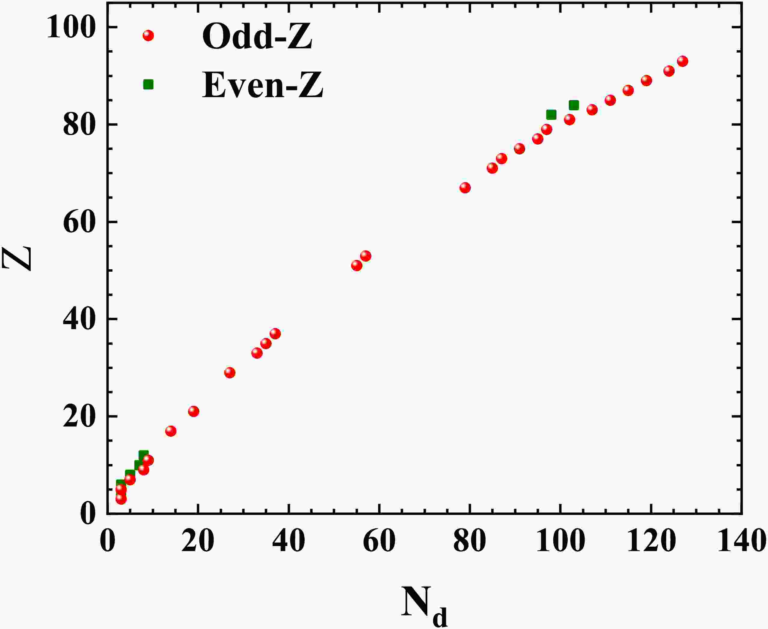
        Fig. 1 illustrates the relationship between proton number and neutron number for proton drip-line nuclei, as determined from the experimental values in the AME2020 [35]. Red dots correspond to drip-line nuclei with odd-Z, while green squares represent those with even-Z. For odd-Z nuclei, the proton drip-line positions are defined by $ S_{{\rm{p}}} $, indicating the nuclei beyond the proton drip-line are unstable to direct proton emission from their ground state. For even-Z nuclei, the drip-line is determined by $ S_{\rm{2p}} $. When $ S_{\rm{2p}} \lt 0 $, the simultaneous emission of two protons is energetically allowed, the nucleus may remain bound to the emission of a single proton due to pairing effects. Thus, the even-Z drip-line is often located one or two protons beyond the odd-Z drip-line. Compared to even-Z isotopes, a larger number of odd-Z isotopes have their proton drip-line positions determined by experimentally measured nuclear masses listed in the AME2020. Therefore, our analysis will focus on the drip-line positions and systematic trends for odd-Z nuclei.
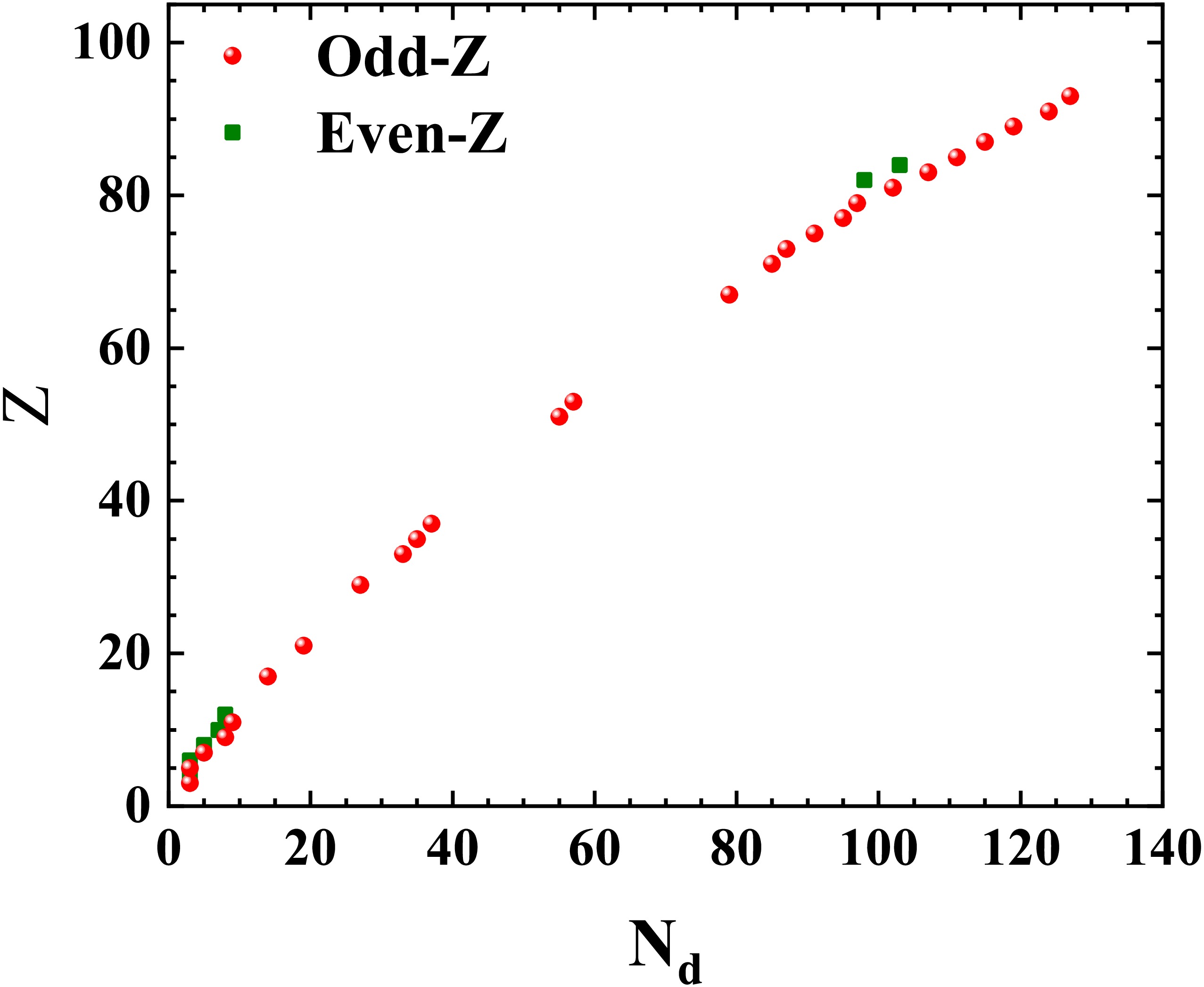
        Figure 1.  (color online) Proton drip-line nuclei determined with the measured nuclear mass dada listed in the AME2020 [35]. The red and green symbles are those for the odd-Z and even-Z isotopes, respectively.

        From the proton drip-line to beyond it, nuclear properties transition from being ”marginally bound” to ”loosely bound” and exhibit significant changes in their dominant decay modes and half-lives. We analyzed the systematic variation of half-lives along odd-Z isotopic chains for both drip-line nuclei with $ Z \leq 81 $, as determined by the AME2020 above, and their first unbound neighbors. The experimental half-life data are taken from Ref. [36], and the logarithms of $ T_{1/2} $ are presented in Fig. 2, in which the upward and downward arrows indicate the lower and upper limits of half-life. We can see that for nuclei with $ Z \lt 50 $, the dominant decay mode shifts from β-decay inside the drip-line to direct proton emission beyond it, potentially leading to an orders-of-magnitude variation in half-lives, except for the cases of copper (Cu) and arsenic (As) which primary decay modes both are β-decay inside and beyond the drip-line. For heavier nuclei with $ Z \gt 50 $, the Coulomb barrier gradually increases and the competition mechanism among various decay modes becomes more complex due to the emergence of α-decay and spontaneous fission. Consequently, the orders-of-magnitude difference in half-lives between bound and unbound nuclei near the drip-line diminishes with increasing proton number Z. Naturally, for odd-Z isotopic chains with $ Z \lt 50 $, we can infer the locations of proton drip-line nuclei, which cannot be directly determined solely by nuclear mass data, by analyzing experimentally observed changes in decay modes and the measured orders-of-magnitude jumps in half-lives.
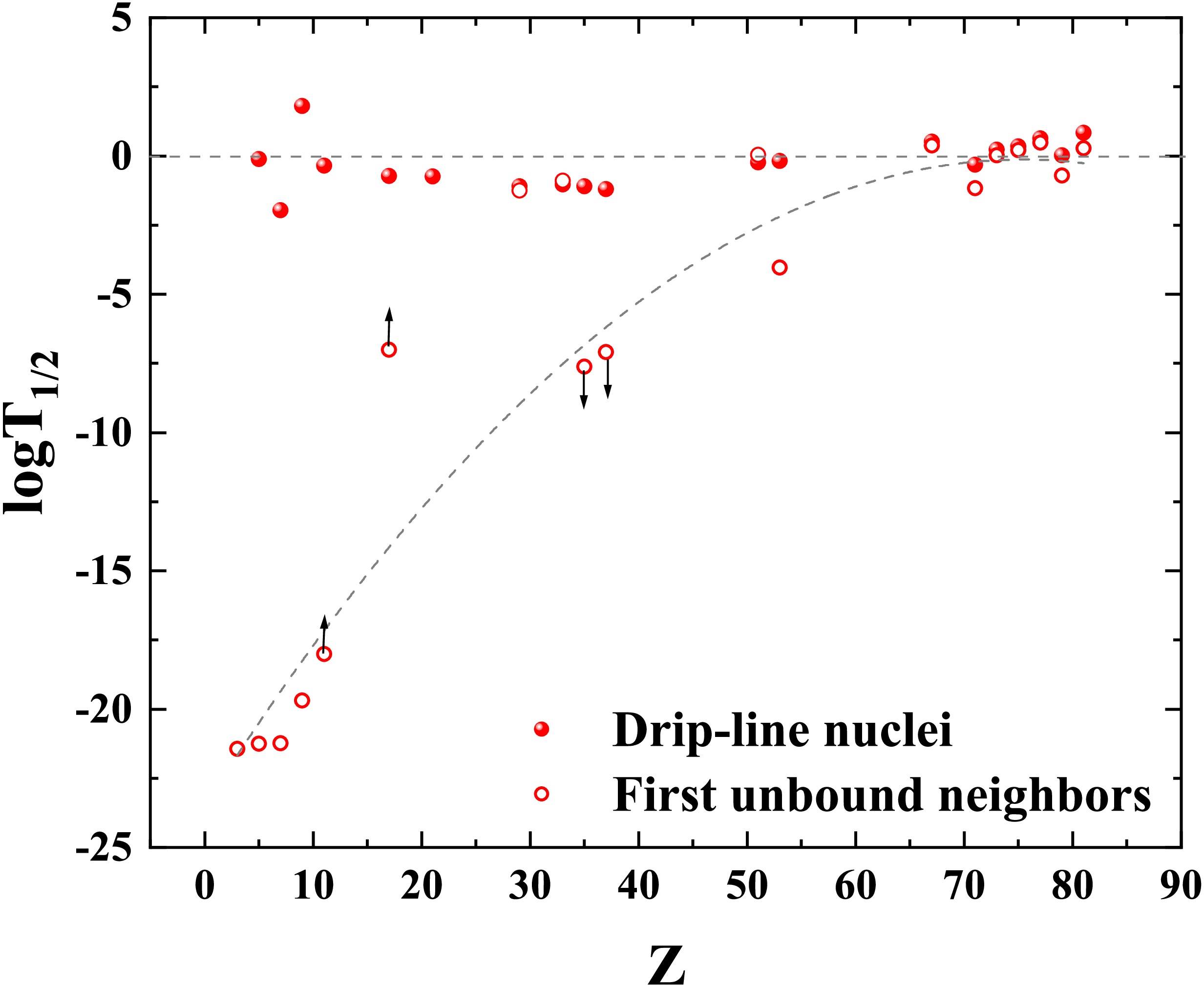
        Figure 2.  (color online) Logarithms of half-lives $ T_{1/2} $ [36] of proton drip-line nuclei for $ Z \leq 81 $ with neutron number $ N_{{\rm{d}}} $ and their first unbound neighbors with $ N_{{\rm{d}}}-1 $ along the isotopic chains. Upward arrows indicate the lower limit of half-life, and downward arrows the upper limit. The dashed curves are to guide to the eyes.

      II.   CRITERION FOR THE PROTON DRIP-LINE
      • Proton drip-line nuclei represent the boundary of nuclides where the one-proton separation energy $ S_{{\rm{p}}} $ approaches zero:

        $ S_{{\rm{p}}}(Z,N) = B(Z,N) - B(Z-1, N) = 0, $

        (1)

        where $ B(Z,N) $ denotes the binding energy of a nucleus with proton number Z and neutron number N. Considering if the two-proton separation energy

        $ S_{\rm{2p}}(Z,N) = B(Z, N)- B(Z-2, N) \lt 0 $

        (2)

        while $ S_{{\rm{p}}} \gt 0 $, the nucleus may undergo two-proton radioactivity. The location of proton drip-line nuclei is defined by the one- and two- proton separation energies. We will determine the proton drip-line by examining nuclei along isotopic chains. For a given number of protons (Z), the proton drip-line nucleus is the one with the lowest number of neutrons (N) that remains bound with respect to the emission of one or two protons. The drip-line nuclei ($ Z,N_{{\rm{d}}} $) are empirically identified where the separation energies $ S_{{\rm{p}}} $ and $ S_{\rm{2p}} $ are positive, meanwhile, one of the $ S_{{\rm{p}}} $ or $ S_{\rm{2p}} $ of the first unbound neighbors ($ Z,N_{{\rm{d}}}-1 $) is negative:

        $ \begin{cases} S_{{\rm{p}}}(Z,N_{{\rm{d}}}) \gt 0 & {\rm{and}}\; \; \; \; S_{\rm{2p}}(Z,N_{{\rm{d}}}) \gt 0 \\ S_{{\rm{p}}}(Z,N_{{\rm{d}}}-1) \lt 0 & {\rm{or}}\; \; \; \; S_{\rm{2p}}(Z,N_{{\rm{d}}}-1) \lt 0 . \end{cases} $

        (3)

        Fig. 1 illustrates the relationship between proton number and neutron number for proton drip-line nuclei, as determined from the experimental values in the AME2020 [35]. Red dots correspond to drip-line nuclei with odd-Z, while green squares represent those with even-Z. For odd-Z nuclei, the proton drip-line positions are defined by $ S_{{\rm{p}}} $, indicating the nuclei beyond the proton drip-line are unstable to direct proton emission from their ground state. For even-Z nuclei, the drip-line is determined by $ S_{\rm{2p}} $. When $ S_{\rm{2p}} \lt 0 $, the simultaneous emission of two protons is energetically allowed, the nucleus may remain bound to the emission of a single proton due to pairing effects. Thus, the even-Z drip-line is often located one or two protons beyond the odd-Z drip-line. Compared to even-Z isotopes, a larger number of odd-Z isotopes have their proton drip-line positions determined by experimentally measured nuclear masses listed in the AME2020. Therefore, our analysis will focus on the drip-line positions and systematic trends for odd-Z nuclei.

        Figure 1.  (color online) Proton drip-line nuclei determined with the measured nuclear mass dada listed in the AME2020 [35]. The red and green symbles are those for the odd-Z and even-Z isotopes, respectively.

        From the proton drip-line to beyond it, nuclear properties transition from being ”marginally bound” to ”loosely bound” and exhibit significant changes in their dominant decay modes and half-lives. We analyzed the systematic variation of half-lives along odd-Z isotopic chains for both drip-line nuclei with $ Z \leq 81 $, as determined by the AME2020 above, and their first unbound neighbors. The experimental half-life data are taken from Ref. [36], and the logarithms of $ T_{1/2} $ are presented in Fig. 2, in which the upward and downward arrows indicate the lower and upper limits of half-life. We can see that for nuclei with $ Z \lt 50 $, the dominant decay mode shifts from β-decay inside the drip-line to direct proton emission beyond it, potentially leading to an orders-of-magnitude variation in half-lives, except for the cases of copper (Cu) and arsenic (As) which primary decay modes both are β-decay inside and beyond the drip-line. For heavier nuclei with $ Z \gt 50 $, the Coulomb barrier gradually increases and the competition mechanism among various decay modes becomes more complex due to the emergence of α-decay and spontaneous fission. Consequently, the orders-of-magnitude difference in half-lives between bound and unbound nuclei near the drip-line diminishes with increasing proton number Z. Naturally, for odd-Z isotopic chains with $ Z \lt 50 $, we can infer the locations of proton drip-line nuclei, which cannot be directly determined solely by nuclear mass data, by analyzing experimentally observed changes in decay modes and the measured orders-of-magnitude jumps in half-lives.

        Figure 2.  (color online) Logarithms of half-lives $ T_{1/2} $ [36] of proton drip-line nuclei for $ Z \leq 81 $ with neutron number $ N_{{\rm{d}}} $ and their first unbound neighbors with $ N_{{\rm{d}}}-1 $ along the isotopic chains. Upward arrows indicate the lower limit of half-life, and downward arrows the upper limit. The dashed curves are to guide to the eyes.

      III.   PROTON DRIP-LINE NUCLEI DEDUSED FROM HALF-LIFE
      • For the odd-Z isotopic chains with $ Z<50 $, if a transition in the dominant decay mode from β decay to one-proton emission is observed toward the neutron-deficient side, the corresponding half-lives may plunge from the millisecond range to the nanosecond scale or even lower, as shown in Fig. 3(a). The red symbols in Fig. 3(a) correspond to the proton drip-line nuclei obtained above and their first proton-emitting neighbors. The blue symbols represent those odd-Z nuclei for which the proton drip-line location has not yet been definitively determined, the solid and hollow symbols corresponding to β-decay nuclei and their first candidate proton emitters respectively. For the first possible one-proton emitter on an isotopic chain, the range of proton emission energy $ Q_{{\rm{p}}} $, can be deduced from its experimentally observed limit of half-life via the quantum tunneling model. A positive $ Q_{{\rm{p}}} $ (indicating $ S_{{\rm{p}}} \lt 0 $) allows the nucleus adjacent to this transition point to be identified as the prospective proton drip-line nucleus, whose $ S_{{\rm{p}}} $ is either measured or predicted to be greater than zero.
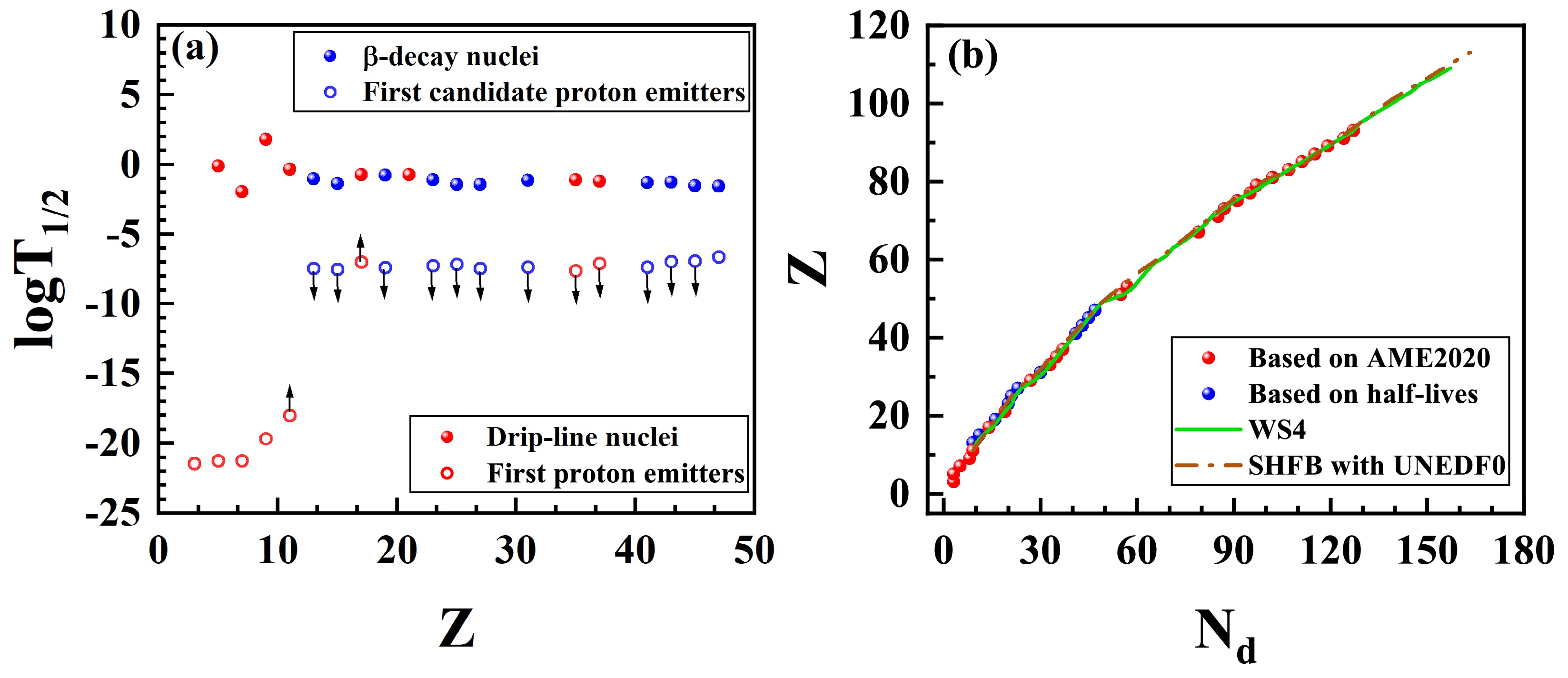
        Figure 3.  (color online) (a). The same as Fig. 2, but for isotopic chains with $ Z<50 $. (b). The same as Fig. 1, but inserting the prospective proton drip-line nuclei with half-life imformation.

        Analogous to α-decay, one-proton emission can be conceptualized as the quantum tunneling of the emitted proton through the potential barrier between itself and the daughter nucleus. The proton emission energy $ Q_{{\rm{p}}} $ can be deduced from the half-life $ T_{1/2}^{{\rm{p}}} $ by using a Gamow-like model[32, 33], originally developed for α-decay. Based on the expression of the proton emission half-life $ T_{1/2}^{{\rm{p}}} $

        $ T_{1/2}^{{\rm{p}}}=\frac{\ln2}{\nu P}, $

        (4)

        one can calculate the value of penetration probability P directely, in which ν is the collision frequency of the emitted proton with the barrier. As an approximation, the harmonic oscillator frequency adopted from Ref.[32] is utilized in our calculations:

        $ h\nu=\hbar \omega \backsimeq \frac{41}{A^{1/3}}\; {\rm{MeV}}, $

        (5)

        where A denotes the mass number of the parent nucleus. Within the framework of the WKB approximation, the penetration probability P can be expressed as

        $ P=\exp\left[-\frac{2}{\hbar}\int_{R}^{R_{c}}\sqrt{2\mu\left[V(r)-Q_{{\rm{p}}}\right]}\; \mathrm{d}r\right]. $

        (6)

        The interaction potential $ V(r) $ between the emitted proton with orbital angular momentum l and the daughter nucleus is given as

        $ V(r)= \begin{cases} -V_0, & 0 \leq r \leq R \\ \frac{1(Z-1) e^2}{4\pi \varepsilon_0 r} + \frac{\hbar^2 l(l+1)}{2\mu r^2}, & r \gt R \end{cases} $

        (7)

        Z is the proton number of the parent nucleus, and $ V_0 $ represents the depth of the nuclear potential well, when $ r \gt R $ the total potential includes contributions from both the Coulomb and the centrifugal parts. In the expressions (6) and (7), $ \mu = m_p m_{A-1}/(m_p + m_{A-1}) $ is the reduced mass of the proton-daughter system and R is the inner classical turning radius, customarily taken as the sum of the radii of the proton and the daughter nucleus $ R = 1.20\left[1^{1/3} + (A-1)^{1/3}\right] {\rm{fm}} $. $ R_c $ denotes the outer classical turning radius which is determined by the condition $ \dfrac{1(Z-1) e^2}{4\pi \varepsilon_0 R_c} + \dfrac{\hbar^2 l(l+1)}{2\mu R_c^2} = Q_{{\rm{p}}} $, and is calculated by

        $ R_c=\frac{R_{c_0}}{2} \left( 1 + \sqrt{1 + \frac{2l(l+1)\hbar^2 }{\mu R_{c_0}^2 Q_{{\rm{p}}}}} \right), $

        (8)

        where $ R_{c_0} = \dfrac{(Z-1)e^2}{4\pi \varepsilon_0 Q_{{\rm{p}}}} $ is the outer classical turning radius for the case of $ l = 0 $. In our calculations, the orbital angular momentum l of the emitted proton is determined by the conservation of parity and angular momentum of the system before and after proton emission. The proton emission energy $ Q_{{\rm{p}}} $ is obtained by integrating expression (6), where the penetration probability P is taken as a known input parameter.

        As a test of our calculations, we compute the $ Q_{{\rm{p}}_{\rm{l}}}^{{\rm{G}}} $ values for proton-emitting nuclei whose half-lives and separation energies have been experimentally measured. A comparison with the experimental results is made, and the corresponding data are listed in Table 1. The experimetal data of $ j^{\pi} $ used to determine the angular momentum l of the emitted proton, $ T_{1/2}^{{\rm{p}}} $ and $ S_{{\rm{p}}} $ are taken from Ref.[35, 36]. For reference, the corresponding results $ Q_{{\rm{p}}_{\rm{l}}}^{\rm{R}} $ calculated via the standard R-matrix expression [11] are also listed in Table 1. Under this method, the value of penetration probability P are obtained by the following expression [11]

        Nuclide $ j^{\pi} $ l Half-life (s) $ S_{{\rm{p}}}\; \; ({\rm{keV}}) $ $ Q_{{\rm{p}}_{\rm{l}}}^{\rm{G}}\; ({\rm{keV}})$ $ Q_{{\rm{p}}_{\rm{l}}}^{\rm{R}} \; ({\rm{keV}})$ $ Q_{{\rm{p}}_0}^{\rm{G}}\; ({\rm{keV}})$ $ Q_{{\rm{p}}_0}^{\rm{R}} \; ({\rm{keV}})$
        $ ^{5} {\rm{Li}}$ $ 3/2^{-} $ 1 $ 3.7\times 10^{-22} $ $ -1960 \pm 50 $ 2081 1207 279 172
        $ ^{7} {\rm{B}}$ $ 3/2^{-} $ 1 $ 5.7\times 10^{-22} $ $ -2013 \pm 26 $ 1905 1359 579 436
        $ ^{9} {\rm{B}}$ $ 3/2^{-} $ 1 $ 8.0\times 10^{-19} $ $ -185.8 \pm 0.9 $ 173 154 92 84
        $ ^{11} {\rm{N}}$ $ 1/2^{+} $ 0 $ 5.85\times 10^{-22} $ $ -1378 \pm 5 $ 972 813 972 813
        $ ^{15} {\rm{F}}$ $ 1/2^{+} $ 0 $ 1.1\times 10^{-21} $ $ -1270 \pm 14 $ 1110 1001 1110 1001
        $ ^{16} {\rm{F}}$ $ 0^{-} $ 0 $ 2.1\times 10^{-20} $ $ -531 \pm 5 $ 538 506 538 506
        $ ^{19} {\rm{N}}{\rm{a}}$ $ 5/2^{+} $ 2 $> 1.0\times 10^{-18} $ $ -323 \pm 11 $ $< 901 $ $< 864 $ $< 403 $ $< 390 $
        $ ^{30} {\rm{Cl}}$ $ 3^{+}\# $ 2 $> 1.0\times 10^{-7} $ $ -480 \pm 20 $ $< 167 $ $< 166 $ $< 133 $ $< 132 $
        $ ^{69} {\rm{B}}{\rm{r}}$ $ 5/2^{-} $ 3 $< 2.4\times 10^{-8} $ $ -640 \pm 40 $ $> 657 $ $> 664 $ $> 508 $ $> 513 $
        $ ^{73} {\rm{Rb}}$ $ 3/2^{-}\# $ 1 $< 8.1\times 10^{-8} $ $ -640 \pm 40 $ $> 552 $ $> 558 $ $> 530 $ $> 535 $
        $ ^{109} {\rm{I}}$ $ 3/2^{+} $ 2 $ 9.28\times 10^{-5} $ $ -820 \pm 4 $ 796 806 737 746
        $ ^{112} {\rm{Cs}}$ $ 1^{+}\# $ 2 $ 4.9\times 10^{-4} $ $ -816 \pm 4 $ 797 808 741 751
        $ ^{113} {\rm{Cs}}$ $ 3/2^{+} $ 2 $ 1.694\times 10^{-5} $ $ -972.8 \pm 2.2 $ 895 908 829 840
        $ ^{117} {\rm{La}}$ $ 3/2^{+} $ 2 0.0217 $ -820 \pm 3 $ 746 755 697 706
        $ ^{121} {\rm{P}}{\rm{r}}$ $ 3/2^{+}\# $ 2 0.012 $ -890 \pm 10 $ 803 813 752 761
        $ ^{131} {\rm{Eu}}$ $ 3/2^{+} $ 2 0.0178 $ -947 \pm 5 $ 875 887 823 834
        $ ^{135} {\rm{Tb}}$ $ 7/2^{-} $ 3 0.00101 $ -1188 \pm 7 $ 1073 1089 948 962
        $ ^{141} {\rm{Ho}}$ $ 7/2^{-} $ 3 0.0041 $ -1177 \pm 7 $ 1072 1088 953 966
        $ ^{145} {\rm{Tm}}$ $ 11/2^{-} $ 5 $ 3.17\times 10^{-6} $ $ -1736 \pm 7 $ 1716 1747 1254 1275
        $ ^{146} {\rm{Tm}}$ $ 1^{+} $ 0 0.155 $ -896 \pm 6 $ 898 910 898 910
        $ ^{147} {\rm{Tm}}$ $ 11/2^{-} $ 5 0.58 $ -1059 \pm 3 $ 1063 1078 822 832
        $ ^{150} {\rm{Lu}}$ $ 10/2^{-} $ 5 0.0045 $ -1269.6 \pm 2.3 $ 1372 1395 1042 1058
        $ ^{155} {\rm{Ta}}$ $ 11/2^{-} $ 5 0.0032 $ -1453 \pm 15 $ 1440 1464 1100 1116
        $ ^{156} {\rm{Ta}}$ $ 2^{-} $ 2 0.106 $ -1020 \pm 4 $ 1037 1052 984 998
        $ ^{157} {\rm{Ta}}$ $ 1/2^{+} $ 0 0.0101 $ -935 \pm 10 $ 965 978 965 978
        $ ^{160} {\rm{Re}}$ $ 4^{-} $ 2 $ 6.11\times 10^{-4} $ $ -1267 \pm 7 $ 1269 1289 1202 1220
        $ ^{161} {\rm{Re}}$ $ 1/2^{+} $ 0 $ 4.4\times 10^{-4} $ $ -1197 \pm 5 $ 1217 1236 1217 1236
        $ ^{166} {\rm{I}}{\rm{r}}$ $ 2^{-} $ 2 0.0105 $ -1152 \pm 8 $ 1125 1142 1071 1086
        $ ^{167} {\rm{I}}{\rm{r}}$ $ 1/2^{+} $ 0 0.0293 $ -1070 \pm 4 $ 1091 1107 1091 1107
        $ ^{170} {\rm{Au}}$ $ 2^{-} $ 2 $ 2.9\times 10^{-4} $ $ -1472 \pm 12 $ 1404 1427 1332 1353
        $ ^{171} {\rm{Au}}$ $ 1/2^{+} $ 0 $ 2.23\times 10^{-5} $ $ -1448 \pm 10 $ 1446 1470 1446 1470
        $ ^{177} {\rm{Tl}}$ $ 1/2^{+} $ 0 0.018 $ -1156 \pm 19 $ 1180 1198 1180 1198

        Table 1.  Comparison of the calculated proton emission energies $ Q_{{\rm{p}}_{\rm{l}}}^{\rm{G}} $ with the measured proton separation energies. For reference, the corresponding results $ Q_{{\rm{p}}_{\rm{l}}}^{\rm{R}} $ calculated via the standard R-matrix method are also listed. The experimetal data of $ j^{\pi} $, $ T_{1/2}^{{\rm{p}}} $ and $ S_{{\rm{p}}} $ are taken from Ref.[35, 36]. $ Q_{{\rm{p}}_0}^{\rm{G}} $ and $ Q_{{\rm{p}}_0}^{\rm{R}} $ are the corresponding results when the angular momentum l is taken as zero.

        $ P = \frac{\mu r_{\rm{ch}}^2 \ln2}{\hbar \theta^2 T_{1/2}^{{\rm{p}}}} $

        (9)

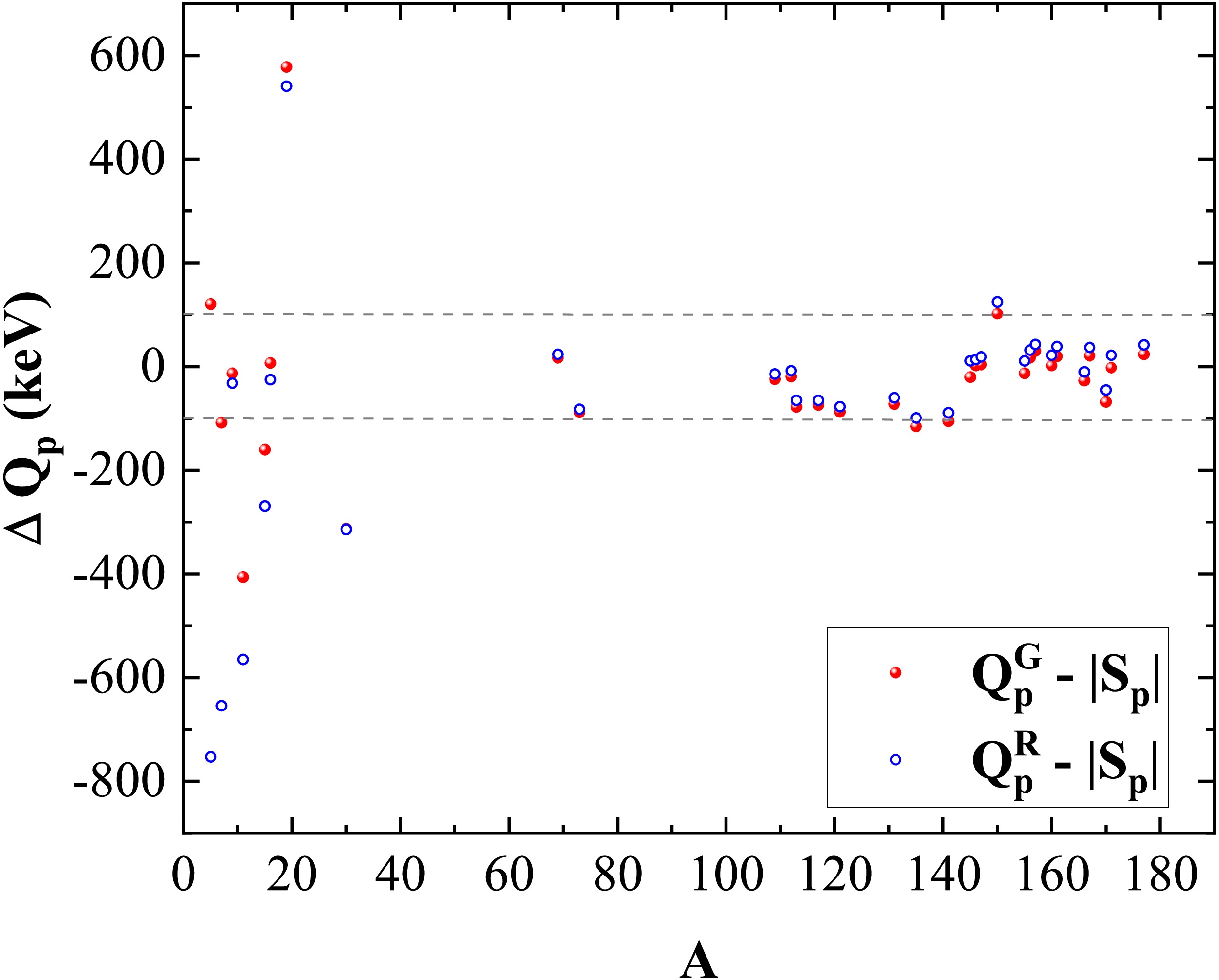
        with $ \theta^2 = 1 $ and $ r_{\rm{ch}} = 1.4 A^{1/3} {\rm{fm}} $. Then, solve for $ Q_{{\rm{p}}_{\rm{l}}}^{\rm{R}} $ by combining equation (9) and equation (6). Fig. 4 shows the deviation between the calculated values $ Q_{{\rm{p}}} $ and the experimentally measured $ S_{{\rm{p}}} $ values $ \Delta Q_{{\rm{p}}} = Q_{{\rm{p}}}^{\rm{G/R}} - |S_{{\rm{p}}}| $. For medium-mass proton emitters, the majority of deviations $ \Delta Q_{{\rm{p}}} $ obtained from both the Gamow-like and R-matrix calculations are within $ 100 $ keV of the experimental values. For light proton emitters with $ A \lt 20 $, the results from the Gamow-like method are in better agreement with the experimental data. Our calculations show that taking the angular momentum l of the emitted proton properly into account leads to a significant improvement in the calculated $ Q_{{\rm{p}}} $ for light proton emitters. As shown in the last two columns of Table 1, $ Q_{{\rm{p}}_0}^{{\rm{G}}} $ and $ Q_{{\rm{p}}_0}^{{\rm{R}}} $ are the calculation results obtained by setting $ l = 0 $. Without the centrifugal barrier, the calculated $ Q_{{\rm{p}}} $ for light nuclei with $ A \lt 20 $ is $ 1 \sim 2 $ MeV lower than the experimentally measured $ |S_{{\rm{p}}}| $. With the inclusion of its contribution, the $ Q_{{\rm{p}}} $ values are significantly increased. This is because light nuclei have a relatively low Coulomb barrier, and the centrifugal contribution significantly raises the effective barrier height that the emitted proton should tunnel through. Furthermore, when the centrifugal term is included, the outer turning radius increases correspondingly, which means the width of the barrier also becomes larger. For a given penetration probability, the proton therefore requires a higher emission energy.

        Figure 4.  (color online) Deviation between the calculated values $ Q_{\rm{p}} $ and the experimentally measured $ S_{\rm{p}} $ values. The two gray dashed lines correspond to $ \Delta Q_{\rm{p}} = \pm 100 $ keV respectively.

        Furthermore, we calculate the lower limit of $ Q_{{\rm{p}}} $ for the nuclei corresponding to the blue hollow circles in Fig. 3(a), i.e., $ ^{21} {\rm{Al}}$, $ ^{25} {\rm{P}}$, $ ^{34} {\rm{K}}$, $ ^{42} {\rm{V}}$, $ ^{45} {\rm{Mn}}$, $ ^{49} {\rm{Co}}$, $ ^{59} {\rm{Ga}}$, $ ^{81} {\rm{Nb}}$, $ ^{85} {\rm{Tc}}$, $ ^{89} {\rm{Rh}}$, $ ^{93} {\rm{Ag}}$. These nuclei represent the first candidate proton emitters along their respective isotopic chains toward the neutron deficient side. The calculation results are presented in Table 2. Due to the lack of measured $ j^{\pi} $, the values of l can only be deduced from the evaluated data in Ref. [36], and are marked with the symbol “#” in the table. Since we are concerned with the lower limit of $ Q_{{\rm{p}}} $ for these nuclei, it is reasonable to set l to zero, obtaining a lower value $ Q_{{\rm{p}}_0} $. In this way the determination of the sign of $ Q_{{\rm{p}}} $ is not affected. The calculation results suggest that these nuclei are unbound, and the nuclides exhibiting a sharp drop in half-life, i.e., $ ^{22} {\rm{Al}}$, $ ^{26} {\rm{P}}$, $ ^{35} {\rm{K}}$, $ ^{43} {\rm{V}}$, $ ^{46} {\rm{Mn}}$, $ ^{50} {\rm{Co}}$, $ ^{60} {\rm{Ga}}$, $ ^{82} {\rm{Nb}}$, $ ^{86} {\rm{Tc}}$, $ ^{90} {\rm{Rh}}$, $ ^{94} {\rm{Ag}}$ are suggested to be the proton drip-line nuclei on their respective isotopic chains, shown in Fig 3(b) with blue dots. For the case of $ ^{35} {\rm{K}}$, $ ^{43} {\rm{V}}$, $ ^{46} {\rm{Mn}}$, $ ^{50} {\rm{Co}}$, the measured proton separation energies $ S_{{\rm{p}}} $ have been pronounced to be posibive in AME2020. Recent nuclear mass measurements reported in Refs. [37] and [38] give the proton separation energies for $ ^{22} {\rm{Al}}$ as $ S_{{\rm{p}}} = 100.4 $ keV and $ S_{{\rm{p}}} = 90 $ keV, respectively. Ref. [38] also reports $ S_{{\rm{p}}} = 118 $ keV for $ ^{26} {\rm{P}}$. Furthermore, the new ground-state mass measurement of $ ^{60} {\rm{Ga}}$ in Ref. [39] yields $ S_{{\rm{p}}} = 108 $ keV. The newly measured mass of $ ^{95} {\rm{Ag}}$ is reported in Ref. [40], yielding a positive $ S_{{\rm{p}}} = 930 $ keV. While no experimental mass has been reported for $ ^{94} {\rm{Ag}}$, the Configuration-Interaction Shell Model (CISM) [41] predicts an increased binding energy for this nucleus due to proton-neutron pairing enhancement. Fig. 3(b) simultaneously presents the proton drip-line obtained from the WS4 nuclear mass model[42] and the Skyrme Hartree-Fock-Bogoliubov method (SHFB) with UNEDF0 interaction [6]. The results of both methods coincide with the positions of the blue points identified through our half-life analysis. An alternative approach to determining the proton drip-line locations for odd-Z nuclei with $ Z \lt 50 $ is to utilize experimentally measured half-lives and decay mode information.

        Nuclide $ j^{\pi}(\#) $ $ l(\#) $ Half-life (s) $ Q_{{\rm{p}}_{\rm{l}}}^{\rm{G}}\; ({\rm{keV}}) $ $ Q_{{\rm{p}}_{\rm{l}}}^{\rm{R}} \; ({\rm{keV}})$ $ Q_{{\rm{p}}_0}^{\rm{G}} \; ({\rm{keV}})$ $ Q_{{\rm{p}}_0}^{\rm{R}}\; ({\rm{keV}}) $
        $ ^{21} {\rm{Al}}$ $ 5/2^{+} $ 2 $< 3.5\times 10^{-8} $ $> 112 $ $> 110 $ $> 83 $ $> 82 $
        $ ^{25} {\rm{P}}$ $ 1/2^{+} $ 0 $< 3.0\times 10^{-8} $ $> 111 $ $> 110 $ $> 111 $ $> 110 $
        $ ^{34} {\rm{K}}$ $ 1^{+} $ 0 $< 4.0\times 10^{-8} $ $> 170 $ $> 170 $ $> 170 $ $> 170 $
        $ ^{42} {\rm{V}}$ $ 2^{-} $ 3 $< 5.5\times 10^{-8} $ $> 341 $ $> 342 $ $> 237 $ $> 238 $
        $ ^{45} {\rm{Mn}}$ $ 5/2^{-} $ 3 $< 7.0\times 10^{-8} $ $> 382 $ $> 383 $ $> 273 $ $> 274 $
        $ ^{49} {\rm{Co}}$ $ 7/2^{-} $ 3 $< 3.5\times 10^{-8} $ $> 444 $ $> 446 $ $> 322 $ $> 324 $
        $ ^{59} {\rm{Ga}}$ $ 3/2^{-} $ 1 $< 4.3\times 10^{-8} $ $> 424 $ $> 428 $ $> 404 $ $> 407 $
        $ ^{81} {\rm{Nb}}$ $ 9/2^{+} $ 4 $< 4.4\times 10^{-8} $ $> 927 $ $> 939 $ $> 644 $ $> 652 $
        $ ^{85} {\rm{Tc}}$ $ 1/2^{-} $ 1 $< 1.1\times 10^{-7} $ $> 695 $ $> 704 $ $> 671 $ $> 679 $
        $ ^{89} {\rm{Rh}}$ $ 9/2^{+} $ 4 $< 1.2\times 10^{-7} $ $> 1001 $ $> 1015 $ $> 720 $ $> 729 $
        $ ^{93} {\rm{Ag}}$ $ 9/2^{+} $ 4 $ 2.28\times 10^{-7} $ $ 1031 $ $ 1046 $ $ 754 $ $ 763 $

        Table 2.  Lower limit of $ Q_{{\rm{p}}} $ for the candidate proton emitters. $ Q_{{\rm{p}}_{\rm{l}}}^{\rm{G/R}} $ denotes the result obtained by including the centrifugal term, whereas$ Q_{{\rm{p}}_0}^{\rm{G/R}} $ corresponds to the case where $ l = 0 $.

        The vast majority of proton drip-line nuclei exhibit odd-odd characteristics. Among the 37 odd-Z proton drip-line nuclei shown in Fig. 3(b), only $ ^{17} {\rm{F}}$, $ ^{31} {\rm{Cl}}$,$ ^{35} {\rm{K}}$, $ ^{43} {\rm{V}}$, $ ^{183} {\rm{Tl}}$, $ ^{215} {\rm{P}}$a are odd-even nuclei. Near the proton drip-line, the interaction between unpaired neutrons and protons may provide extra binding energy to compensate for their weakly bound nature[43, 44], making odd-odd nuclei more likely to become proton drip-line nuclei. Possible explanations for the six nuclei with even neutron numbers, include closed-shell and deformation effects. Specifically, $ ^{17} {\rm{F}}$, and $ ^{43} {\rm{V}}$ reside at the neutron magic numbers $ N=8 $ and $ N=20 $, respectively, while $ ^{215} {\rm{P}}$a is near the $ N=126 $ shell closure. For $ ^{31} {\rm{Cl}}$, the $ 1 {\rm{d}}_{5/2} $ neutron subshell closure is relevant, and for $ ^{35} {\rm{K}}$, the $ 2 {\rm{s}}_{1/2} $ subshell closure may play a role[45]. In the case of $ ^{183} {\rm{Tl}}$, deformation effects likely cause a rearrangement of single-particle levels, leading to a deformed subshell closure at $ N=102 $. The competition between odd-odd and odd-even nuclei along the proton drip-line is governed by a balance between the advantage provided by the p-n interaction and shell effects. The former generally stabilizes odd-odd nuclei, while the latter can favor odd-even nuclei at specific neutron numbers. Fig. 5 displays the relation between the neutron-to-proton ($ N_{{\rm{d}}}/Z $) ratio and proton number Z for odd-Z proton drip-line nuclei. An overall increasing trend of the $ N_{{\rm{d}}}/Z $ ratio with Z is presented. Notably, a plateau at $ N_{{\rm{d}}} = Z $ appears in the region $ 33 \leq Z \leq 47 $, which relevants to the rp process in the mass range $ A = 60 \sim 100 $. This plateau likely arises because the valence protons and neutrons occupy similar orbitals, which further enhances the p-n interaction in these odd-odd nuclei.
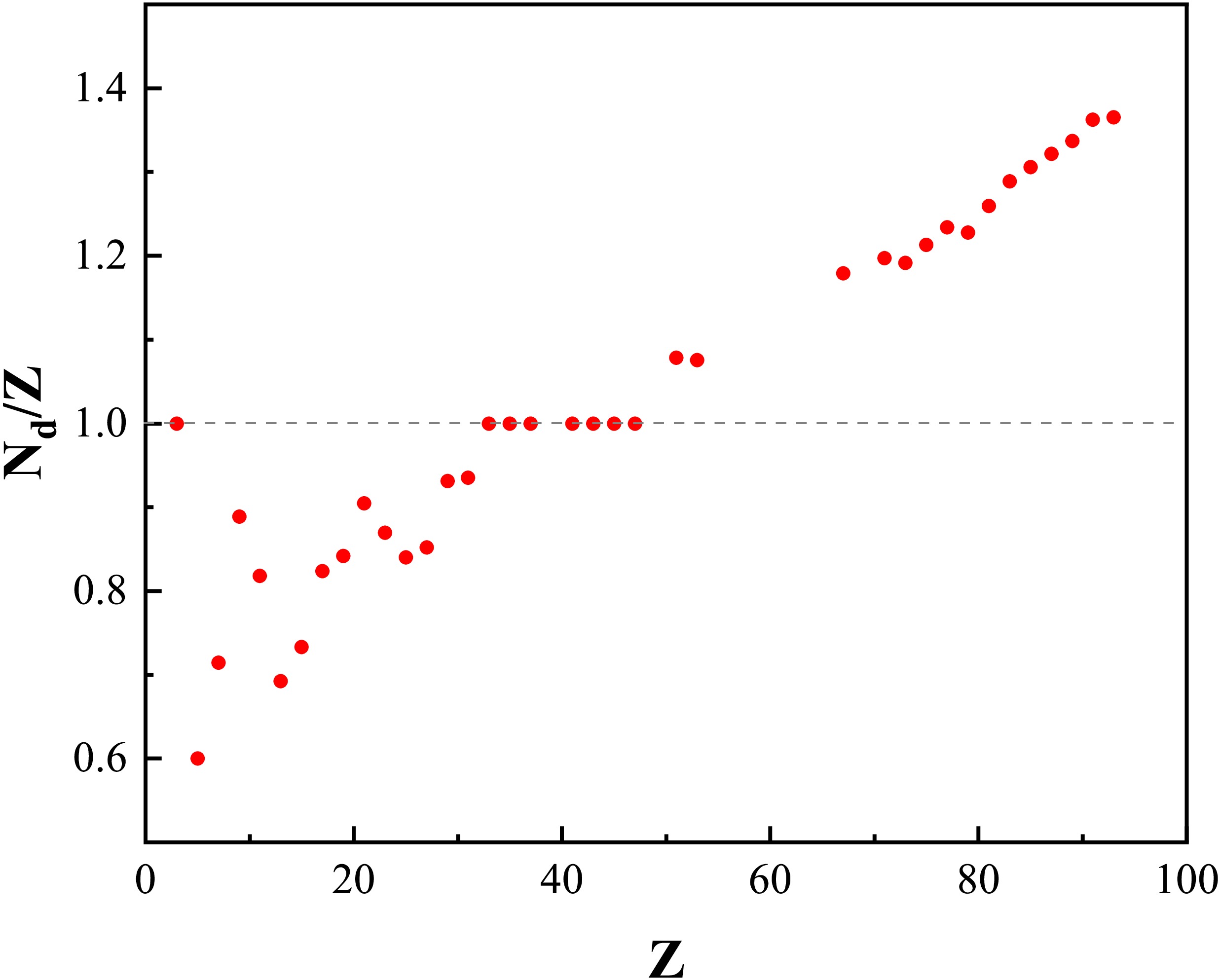
        Figure 5.  (color online) Relation between the neutron-to-proton ($ N_{{\rm{d}}}/Z $) ratio and proton number Z for odd-Z proton drip-line nuclei. The gray dashed line corresponds to the value of $ N_{{\rm{d}}}/Z = 1 $.

      III.   PROTON DRIP-LINE NUCLEI DEDUSED FROM HALF-LIFE
      • For the odd-Z isotopic chains with $ Z<50 $, if a transition in the dominant decay mode from β decay to one-proton emission is observed toward the neutron-deficient side, the corresponding half-lives may plunge from the millisecond range to the nanosecond scale or even lower, as shown in Fig. 3(a). The red symbols in Fig. 3(a) correspond to the proton drip-line nuclei obtained above and their first proton-emitting neighbors. The blue symbols represent those odd-Z nuclei for which the proton drip-line location has not yet been definitively determined, the solid and hollow symbols corresponding to β-decay nuclei and their first candidate proton emitters respectively. For the first possible one-proton emitter on an isotopic chain, the range of proton emission energy $ Q_{{\rm{p}}} $, can be deduced from its experimentally observed limit of half-life via the quantum tunneling model. A positive $ Q_{{\rm{p}}} $ (indicating $ S_{{\rm{p}}} \lt 0 $) allows the nucleus adjacent to this transition point to be identified as the prospective proton drip-line nucleus, whose $ S_{{\rm{p}}} $ is either measured or predicted to be greater than zero.

        Figure 3.  (color online) (a). The same as Fig. 2, but for isotopic chains with $ Z<50 $. (b). The same as Fig. 1, but inserting the prospective proton drip-line nuclei with half-life imformation.

        Analogous to α-decay, one-proton emission can be conceptualized as the quantum tunneling of the emitted proton through the potential barrier between itself and the daughter nucleus. The proton emission energy $ Q_{{\rm{p}}} $ can be deduced from the half-life $ T_{1/2}^{{\rm{p}}} $ by using a Gamow-like model[32, 33], originally developed for α-decay. Based on the expression of the proton emission half-life $ T_{1/2}^{{\rm{p}}} $

        $ T_{1/2}^{{\rm{p}}}=\frac{\ln2}{\nu P}, $

        (4)

        one can calculate the value of penetration probability P directely, in which ν is the collision frequency of the emitted proton with the barrier. As an approximation, the harmonic oscillator frequency adopted from Ref.[32] is utilized in our calculations:

        $ h\nu=\hbar \omega \backsimeq \frac{41}{A^{1/3}}\; {\rm{MeV}}, $

        (5)

        where A denotes the mass number of the parent nucleus. Within the framework of the WKB approximation, the penetration probability P can be expressed as

        $ P=\exp\left[-\frac{2}{\hbar}\int_{R}^{R_{c}}\sqrt{2\mu\left[V(r)-Q_{{\rm{p}}}\right]}\; \mathrm{d}r\right]. $

        (6)

        The interaction potential $ V(r) $ between the emitted proton with orbital angular momentum l and the daughter nucleus is given as

        $ V(r)= \begin{cases} -V_0, & 0 \leq r \leq R \\ \frac{1(Z-1) e^2}{4\pi \varepsilon_0 r} + \frac{\hbar^2 l(l+1)}{2\mu r^2}, & r \gt R \end{cases} $

        (7)

        Z is the proton number of the parent nucleus, and $ V_0 $ represents the depth of the nuclear potential well, when $ r \gt R $ the total potential includes contributions from both the Coulomb and the centrifugal parts. In the expressions (6) and (7), $ \mu = m_p m_{A-1}/(m_p + m_{A-1}) $ is the reduced mass of the proton-daughter system and R is the inner classical turning radius, customarily taken as the sum of the radii of the proton and the daughter nucleus $ R = 1.20\left[1^{1/3} + (A-1)^{1/3}\right] {\rm{fm}} $. $ R_c $ denotes the outer classical turning radius which is determined by the condition $ \dfrac{1(Z-1) e^2}{4\pi \varepsilon_0 R_c} + \dfrac{\hbar^2 l(l+1)}{2\mu R_c^2} = Q_{{\rm{p}}} $, and is calculated by

        $ R_c=\frac{R_{c_0}}{2} \left( 1 + \sqrt{1 + \frac{2l(l+1)\hbar^2 }{\mu R_{c_0}^2 Q_{{\rm{p}}}}} \right), $

        (8)

        where $ R_{c_0} = \dfrac{(Z-1)e^2}{4\pi \varepsilon_0 Q_{{\rm{p}}}} $ is the outer classical turning radius for the case of $ l = 0 $. In our calculations, the orbital angular momentum l of the emitted proton is determined by the conservation of parity and angular momentum of the system before and after proton emission. The proton emission energy $ Q_{{\rm{p}}} $ is obtained by integrating expression (6), where the penetration probability P is taken as a known input parameter.

        As a test of our calculations, we compute the $ Q_{{\rm{p}}_{\rm{l}}}^{{\rm{G}}} $ values for proton-emitting nuclei whose half-lives and separation energies have been experimentally measured. A comparison with the experimental results is made, and the corresponding data are listed in Table 1. The experimetal data of $ j^{\pi} $ used to determine the angular momentum l of the emitted proton, $ T_{1/2}^{{\rm{p}}} $ and $ S_{{\rm{p}}} $ are taken from Ref.[35, 36]. For reference, the corresponding results $ Q_{{\rm{p}}_{\rm{l}}}^{\rm{R}} $ calculated via the standard R-matrix expression [11] are also listed in Table 1. Under this method, the value of penetration probability P are obtained by the following expression [11]

        Nuclide $ j^{\pi} $ l Half-life (s) $ S_{{\rm{p}}}\; \; ({\rm{keV}}) $ $ Q_{{\rm{p}}_{\rm{l}}}^{\rm{G}}\; ({\rm{keV}})$ $ Q_{{\rm{p}}_{\rm{l}}}^{\rm{R}} \; ({\rm{keV}})$ $ Q_{{\rm{p}}_0}^{\rm{G}}\; ({\rm{keV}})$ $ Q_{{\rm{p}}_0}^{\rm{R}} \; ({\rm{keV}})$
        $ ^{5} {\rm{Li}}$ $ 3/2^{-} $ 1 $ 3.7\times 10^{-22} $ $ -1960 \pm 50 $ 2081 1207 279 172
        $ ^{7} {\rm{B}}$ $ 3/2^{-} $ 1 $ 5.7\times 10^{-22} $ $ -2013 \pm 26 $ 1905 1359 579 436
        $ ^{9} {\rm{B}}$ $ 3/2^{-} $ 1 $ 8.0\times 10^{-19} $ $ -185.8 \pm 0.9 $ 173 154 92 84
        $ ^{11} {\rm{N}}$ $ 1/2^{+} $ 0 $ 5.85\times 10^{-22} $ $ -1378 \pm 5 $ 972 813 972 813
        $ ^{15} {\rm{F}}$ $ 1/2^{+} $ 0 $ 1.1\times 10^{-21} $ $ -1270 \pm 14 $ 1110 1001 1110 1001
        $ ^{16} {\rm{F}}$ $ 0^{-} $ 0 $ 2.1\times 10^{-20} $ $ -531 \pm 5 $ 538 506 538 506
        $ ^{19} {\rm{N}}{\rm{a}}$ $ 5/2^{+} $ 2 $> 1.0\times 10^{-18} $ $ -323 \pm 11 $ $< 901 $ $< 864 $ $< 403 $ $< 390 $
        $ ^{30} {\rm{Cl}}$ $ 3^{+}\# $ 2 $> 1.0\times 10^{-7} $ $ -480 \pm 20 $ $< 167 $ $< 166 $ $< 133 $ $< 132 $
        $ ^{69} {\rm{B}}{\rm{r}}$ $ 5/2^{-} $ 3 $< 2.4\times 10^{-8} $ $ -640 \pm 40 $ $> 657 $ $> 664 $ $> 508 $ $> 513 $
        $ ^{73} {\rm{Rb}}$ $ 3/2^{-}\# $ 1 $< 8.1\times 10^{-8} $ $ -640 \pm 40 $ $> 552 $ $> 558 $ $> 530 $ $> 535 $
        $ ^{109} {\rm{I}}$ $ 3/2^{+} $ 2 $ 9.28\times 10^{-5} $ $ -820 \pm 4 $ 796 806 737 746
        $ ^{112} {\rm{Cs}}$ $ 1^{+}\# $ 2 $ 4.9\times 10^{-4} $ $ -816 \pm 4 $ 797 808 741 751
        $ ^{113} {\rm{Cs}}$ $ 3/2^{+} $ 2 $ 1.694\times 10^{-5} $ $ -972.8 \pm 2.2 $ 895 908 829 840
        $ ^{117} {\rm{La}}$ $ 3/2^{+} $ 2 0.0217 $ -820 \pm 3 $ 746 755 697 706
        $ ^{121} {\rm{P}}{\rm{r}}$ $ 3/2^{+}\# $ 2 0.012 $ -890 \pm 10 $ 803 813 752 761
        $ ^{131} {\rm{Eu}}$ $ 3/2^{+} $ 2 0.0178 $ -947 \pm 5 $ 875 887 823 834
        $ ^{135} {\rm{Tb}}$ $ 7/2^{-} $ 3 0.00101 $ -1188 \pm 7 $ 1073 1089 948 962
        $ ^{141} {\rm{Ho}}$ $ 7/2^{-} $ 3 0.0041 $ -1177 \pm 7 $ 1072 1088 953 966
        $ ^{145} {\rm{Tm}}$ $ 11/2^{-} $ 5 $ 3.17\times 10^{-6} $ $ -1736 \pm 7 $ 1716 1747 1254 1275
        $ ^{146} {\rm{Tm}}$ $ 1^{+} $ 0 0.155 $ -896 \pm 6 $ 898 910 898 910
        $ ^{147} {\rm{Tm}}$ $ 11/2^{-} $ 5 0.58 $ -1059 \pm 3 $ 1063 1078 822 832
        $ ^{150} {\rm{Lu}}$ $ 10/2^{-} $ 5 0.0045 $ -1269.6 \pm 2.3 $ 1372 1395 1042 1058
        $ ^{155} {\rm{Ta}}$ $ 11/2^{-} $ 5 0.0032 $ -1453 \pm 15 $ 1440 1464 1100 1116
        $ ^{156} {\rm{Ta}}$ $ 2^{-} $ 2 0.106 $ -1020 \pm 4 $ 1037 1052 984 998
        $ ^{157} {\rm{Ta}}$ $ 1/2^{+} $ 0 0.0101 $ -935 \pm 10 $ 965 978 965 978
        $ ^{160} {\rm{Re}}$ $ 4^{-} $ 2 $ 6.11\times 10^{-4} $ $ -1267 \pm 7 $ 1269 1289 1202 1220
        $ ^{161} {\rm{Re}}$ $ 1/2^{+} $ 0 $ 4.4\times 10^{-4} $ $ -1197 \pm 5 $ 1217 1236 1217 1236
        $ ^{166} {\rm{I}}{\rm{r}}$ $ 2^{-} $ 2 0.0105 $ -1152 \pm 8 $ 1125 1142 1071 1086
        $ ^{167} {\rm{I}}{\rm{r}}$ $ 1/2^{+} $ 0 0.0293 $ -1070 \pm 4 $ 1091 1107 1091 1107
        $ ^{170} {\rm{Au}}$ $ 2^{-} $ 2 $ 2.9\times 10^{-4} $ $ -1472 \pm 12 $ 1404 1427 1332 1353
        $ ^{171} {\rm{Au}}$ $ 1/2^{+} $ 0 $ 2.23\times 10^{-5} $ $ -1448 \pm 10 $ 1446 1470 1446 1470
        $ ^{177} {\rm{Tl}}$ $ 1/2^{+} $ 0 0.018 $ -1156 \pm 19 $ 1180 1198 1180 1198

        Table 1.  Comparison of the calculated proton emission energies $ Q_{{\rm{p}}_{\rm{l}}}^{\rm{G}} $ with the measured proton separation energies. For reference, the corresponding results $ Q_{{\rm{p}}_{\rm{l}}}^{\rm{R}} $ calculated via the standard R-matrix method are also listed. The experimetal data of $ j^{\pi} $, $ T_{1/2}^{{\rm{p}}} $ and $ S_{{\rm{p}}} $ are taken from Ref.[35, 36]. $ Q_{{\rm{p}}_0}^{\rm{G}} $ and $ Q_{{\rm{p}}_0}^{\rm{R}} $ are the corresponding results when the angular momentum l is taken as zero.

        $ P = \frac{\mu r_{\rm{ch}}^2 \ln2}{\hbar \theta^2 T_{1/2}^{{\rm{p}}}} $

        (9)

        with $ \theta^2 = 1 $ and $ r_{\rm{ch}} = 1.4 A^{1/3} {\rm{fm}} $. Then, solve for $ Q_{{\rm{p}}_{\rm{l}}}^{\rm{R}} $ by combining equation (9) and equation (6). Fig. 4 shows the deviation between the calculated values $ Q_{{\rm{p}}} $ and the experimentally measured $ S_{{\rm{p}}} $ values $ \Delta Q_{{\rm{p}}} = Q_{{\rm{p}}}^{\rm{G/R}} - |S_{{\rm{p}}}| $. For medium-mass proton emitters, the majority of deviations $ \Delta Q_{{\rm{p}}} $ obtained from both the Gamow-like and R-matrix calculations are within $ 100 $ keV of the experimental values. For light proton emitters with $ A \lt 20 $, the results from the Gamow-like method are in better agreement with the experimental data. Our calculations show that taking the angular momentum l of the emitted proton properly into account leads to a significant improvement in the calculated $ Q_{{\rm{p}}} $ for light proton emitters. As shown in the last two columns of Table 1, $ Q_{{\rm{p}}_0}^{{\rm{G}}} $ and $ Q_{{\rm{p}}_0}^{{\rm{R}}} $ are the calculation results obtained by setting $ l = 0 $. Without the centrifugal barrier, the calculated $ Q_{{\rm{p}}} $ for light nuclei with $ A \lt 20 $ is $ 1 \sim 2 $ MeV lower than the experimentally measured $ |S_{{\rm{p}}}| $. With the inclusion of its contribution, the $ Q_{{\rm{p}}} $ values are significantly increased. This is because light nuclei have a relatively low Coulomb barrier, and the centrifugal contribution significantly raises the effective barrier height that the emitted proton should tunnel through. Furthermore, when the centrifugal term is included, the outer turning radius increases correspondingly, which means the width of the barrier also becomes larger. For a given penetration probability, the proton therefore requires a higher emission energy.

        Figure 4.  (color online) Deviation between the calculated values $ Q_{\rm{p}} $ and the experimentally measured $ S_{\rm{p}} $ values. The two gray dashed lines correspond to $ \Delta Q_{\rm{p}} = \pm 100 $ keV respectively.

        Furthermore, we calculate the lower limit of $ Q_{{\rm{p}}} $ for the nuclei corresponding to the blue hollow circles in Fig. 3(a), i.e., $ ^{21} {\rm{Al}}$, $ ^{25} {\rm{P}}$, $ ^{34} {\rm{K}}$, $ ^{42} {\rm{V}}$, $ ^{45} {\rm{Mn}}$, $ ^{49} {\rm{Co}}$, $ ^{59} {\rm{Ga}}$, $ ^{81} {\rm{Nb}}$, $ ^{85} {\rm{Tc}}$, $ ^{89} {\rm{Rh}}$, $ ^{93} {\rm{Ag}}$. These nuclei represent the first candidate proton emitters along their respective isotopic chains toward the neutron deficient side. The calculation results are presented in Table 2. Due to the lack of measured $ j^{\pi} $, the values of l can only be deduced from the evaluated data in Ref. [36], and are marked with the symbol “#” in the table. Since we are concerned with the lower limit of $ Q_{{\rm{p}}} $ for these nuclei, it is reasonable to set l to zero, obtaining a lower value $ Q_{{\rm{p}}_0} $. In this way the determination of the sign of $ Q_{{\rm{p}}} $ is not affected. The calculation results suggest that these nuclei are unbound, and the nuclides exhibiting a sharp drop in half-life, i.e., $ ^{22} {\rm{Al}}$, $ ^{26} {\rm{P}}$, $ ^{35} {\rm{K}}$, $ ^{43} {\rm{V}}$, $ ^{46} {\rm{Mn}}$, $ ^{50} {\rm{Co}}$, $ ^{60} {\rm{Ga}}$, $ ^{82} {\rm{Nb}}$, $ ^{86} {\rm{Tc}}$, $ ^{90} {\rm{Rh}}$, $ ^{94} {\rm{Ag}}$ are suggested to be the proton drip-line nuclei on their respective isotopic chains, shown in Fig 3(b) with blue dots. For the case of $ ^{35} {\rm{K}}$, $ ^{43} {\rm{V}}$, $ ^{46} {\rm{Mn}}$, $ ^{50} {\rm{Co}}$, the measured proton separation energies $ S_{{\rm{p}}} $ have been pronounced to be posibive in AME2020. Recent nuclear mass measurements reported in Refs. [37] and [38] give the proton separation energies for $ ^{22} {\rm{Al}}$ as $ S_{{\rm{p}}} = 100.4 $ keV and $ S_{{\rm{p}}} = 90 $ keV, respectively. Ref. [38] also reports $ S_{{\rm{p}}} = 118 $ keV for $ ^{26} {\rm{P}}$. Furthermore, the new ground-state mass measurement of $ ^{60} {\rm{Ga}}$ in Ref. [39] yields $ S_{{\rm{p}}} = 108 $ keV. The newly measured mass of $ ^{95} {\rm{Ag}}$ is reported in Ref. [40], yielding a positive $ S_{{\rm{p}}} = 930 $ keV. While no experimental mass has been reported for $ ^{94} {\rm{Ag}}$, the Configuration-Interaction Shell Model (CISM) [41] predicts an increased binding energy for this nucleus due to proton-neutron pairing enhancement. Fig. 3(b) simultaneously presents the proton drip-line obtained from the WS4 nuclear mass model[42] and the Skyrme Hartree-Fock-Bogoliubov method (SHFB) with UNEDF0 interaction [6]. The results of both methods coincide with the positions of the blue points identified through our half-life analysis. An alternative approach to determining the proton drip-line locations for odd-Z nuclei with $ Z \lt 50 $ is to utilize experimentally measured half-lives and decay mode information.

        Nuclide $ j^{\pi}(\#) $ $ l(\#) $ Half-life (s) $ Q_{{\rm{p}}_{\rm{l}}}^{\rm{G}}\; ({\rm{keV}}) $ $ Q_{{\rm{p}}_{\rm{l}}}^{\rm{R}} \; ({\rm{keV}})$ $ Q_{{\rm{p}}_0}^{\rm{G}} \; ({\rm{keV}})$ $ Q_{{\rm{p}}_0}^{\rm{R}}\; ({\rm{keV}}) $
        $ ^{21} {\rm{Al}}$ $ 5/2^{+} $ 2 $< 3.5\times 10^{-8} $ $> 112 $ $> 110 $ $> 83 $ $> 82 $
        $ ^{25} {\rm{P}}$ $ 1/2^{+} $ 0 $< 3.0\times 10^{-8} $ $> 111 $ $> 110 $ $> 111 $ $> 110 $
        $ ^{34} {\rm{K}}$ $ 1^{+} $ 0 $< 4.0\times 10^{-8} $ $> 170 $ $> 170 $ $> 170 $ $> 170 $
        $ ^{42} {\rm{V}}$ $ 2^{-} $ 3 $< 5.5\times 10^{-8} $ $> 341 $ $> 342 $ $> 237 $ $> 238 $
        $ ^{45} {\rm{Mn}}$ $ 5/2^{-} $ 3 $< 7.0\times 10^{-8} $ $> 382 $ $> 383 $ $> 273 $ $> 274 $
        $ ^{49} {\rm{Co}}$ $ 7/2^{-} $ 3 $< 3.5\times 10^{-8} $ $> 444 $ $> 446 $ $> 322 $ $> 324 $
        $ ^{59} {\rm{Ga}}$ $ 3/2^{-} $ 1 $< 4.3\times 10^{-8} $ $> 424 $ $> 428 $ $> 404 $ $> 407 $
        $ ^{81} {\rm{Nb}}$ $ 9/2^{+} $ 4 $< 4.4\times 10^{-8} $ $> 927 $ $> 939 $ $> 644 $ $> 652 $
        $ ^{85} {\rm{Tc}}$ $ 1/2^{-} $ 1 $< 1.1\times 10^{-7} $ $> 695 $ $> 704 $ $> 671 $ $> 679 $
        $ ^{89} {\rm{Rh}}$ $ 9/2^{+} $ 4 $< 1.2\times 10^{-7} $ $> 1001 $ $> 1015 $ $> 720 $ $> 729 $
        $ ^{93} {\rm{Ag}}$ $ 9/2^{+} $ 4 $ 2.28\times 10^{-7} $ $ 1031 $ $ 1046 $ $ 754 $ $ 763 $

        Table 2.  Lower limit of $ Q_{{\rm{p}}} $ for the candidate proton emitters. $ Q_{{\rm{p}}_{\rm{l}}}^{\rm{G/R}} $ denotes the result obtained by including the centrifugal term, whereas$ Q_{{\rm{p}}_0}^{\rm{G/R}} $ corresponds to the case where $ l = 0 $.

        The vast majority of proton drip-line nuclei exhibit odd-odd characteristics. Among the 37 odd-Z proton drip-line nuclei shown in Fig. 3(b), only $ ^{17} {\rm{F}}$, $ ^{31} {\rm{Cl}}$,$ ^{35} {\rm{K}}$, $ ^{43} {\rm{V}}$, $ ^{183} {\rm{Tl}}$, $ ^{215} {\rm{P}}$a are odd-even nuclei. Near the proton drip-line, the interaction between unpaired neutrons and protons may provide extra binding energy to compensate for their weakly bound nature[43, 44], making odd-odd nuclei more likely to become proton drip-line nuclei. Possible explanations for the six nuclei with even neutron numbers, include closed-shell and deformation effects. Specifically, $ ^{17} {\rm{F}}$, and $ ^{43} {\rm{V}}$ reside at the neutron magic numbers $ N=8 $ and $ N=20 $, respectively, while $ ^{215} {\rm{P}}$a is near the $ N=126 $ shell closure. For $ ^{31} {\rm{Cl}}$, the $ 1 {\rm{d}}_{5/2} $ neutron subshell closure is relevant, and for $ ^{35} {\rm{K}}$, the $ 2 {\rm{s}}_{1/2} $ subshell closure may play a role[45]. In the case of $ ^{183} {\rm{Tl}}$, deformation effects likely cause a rearrangement of single-particle levels, leading to a deformed subshell closure at $ N=102 $. The competition between odd-odd and odd-even nuclei along the proton drip-line is governed by a balance between the advantage provided by the p-n interaction and shell effects. The former generally stabilizes odd-odd nuclei, while the latter can favor odd-even nuclei at specific neutron numbers. Fig. 5 displays the relation between the neutron-to-proton ($ N_{{\rm{d}}}/Z $) ratio and proton number Z for odd-Z proton drip-line nuclei. An overall increasing trend of the $ N_{{\rm{d}}}/Z $ ratio with Z is presented. Notably, a plateau at $ N_{{\rm{d}}} = Z $ appears in the region $ 33 \leq Z \leq 47 $, which relevants to the rp process in the mass range $ A = 60 \sim 100 $. This plateau likely arises because the valence protons and neutrons occupy similar orbitals, which further enhances the p-n interaction in these odd-odd nuclei.

        Figure 5.  (color online) Relation between the neutron-to-proton ($ N_{{\rm{d}}}/Z $) ratio and proton number Z for odd-Z proton drip-line nuclei. The gray dashed line corresponds to the value of $ N_{{\rm{d}}}/Z = 1 $.

      IV.   SUMMARY
      • Based on experimentally measured proton separation energies, as well as decay mode and half-life information, we have determined the proton drip-line locations for odd-Z nuclei. For the odd-Z nuclei with $ Z \lt 50 $, only β-decay and proton emission exist near the drip line. A sharp, orders-of-magnitude decrease in half-life is typically observed immediately beyond the drip-line nucleus along an isotopic chain, corresponding to the transition from β-decay to proton emission. Using the Gamow-like model, we calculate the proton emission energy $ Q_{{\rm{p}}} $ from the proton-emission half-life. This allows us to identify the first candidate proton emitter along an isotopic chain toward the neutron-deficient side and, consequently, to determine the location of the proton drip-line nucleus. $ ^{22} {\rm{Al}}$, $ ^{26} {\rm{P}}$, $ ^{35} {\rm{K}}$, $ ^{43} {\rm{V}}$, $ ^{46} {\rm{Mn}}$, $ ^{50} {\rm{Co}}$, $ ^{60} {\rm{Ga}}$, $ ^{82} {\rm{Nb}}$, $ ^{86} {\rm{Tc}}$, $ ^{90} {\rm{Rh}}$, $ ^{94} {\rm{Ag}}$ are suggested as the proton drip-line nuclei based on the measured half-lives, which coincide with the results of WS4 nuclear mass model and the newly reported mass data of $ ^{22} {\rm{Al}}$, $ ^{26} {\rm{P}}$ and $ ^{60} {\rm{Ga}}$.The odd-odd characteristics and a plateau at $ N_{{\rm{d}}} = Z $ in the region $ 33 \leq Z \leq 47 $ of proton drip-line nuclei are presented. Guided by these two regularities, $ ^{78} {\rm{Y}}$ is likely to be the proton drip-line nucleus for the $ Z = 39 $ isotopic chain. The proton drip-line locations for odd-Z nuclei in the range $ 53 \leq Z \leq 65 $ are not yet definitively established, requiring high-precision experimental measurements or alternative approaches.

        Our calculations indicate that the proper inclusion of the angular momentum l of the emitted proton is essential for accurately calculating the proton emission energy, particularly for light proton emitters. Moreover, we have examined the model dependence by testing two alternative nuclear potentials: the Woods-Saxon potential and the Bass80 potential. Taking $ ^{21} {\rm{Al}}$ as an example, we calculated the penetration probability using the WKB approximation and compared the results with those obtained from the square-well potential. The variation in penetration probability P was found to be within one order of magnitude, and the corresponding change in the extracted $ Q_p $ ​is small.

      IV.   SUMMARY
      • Based on experimentally measured proton separation energies, as well as decay mode and half-life information, we have determined the proton drip-line locations for odd-Z nuclei. For the odd-Z nuclei with $ Z \lt 50 $, only β-decay and proton emission exist near the drip line. A sharp, orders-of-magnitude decrease in half-life is typically observed immediately beyond the drip-line nucleus along an isotopic chain, corresponding to the transition from β-decay to proton emission. Using the Gamow-like model, we calculate the proton emission energy $ Q_{{\rm{p}}} $ from the proton-emission half-life. This allows us to identify the first candidate proton emitter along an isotopic chain toward the neutron-deficient side and, consequently, to determine the location of the proton drip-line nucleus. $ ^{22} {\rm{Al}}$, $ ^{26} {\rm{P}}$, $ ^{35} {\rm{K}}$, $ ^{43} {\rm{V}}$, $ ^{46} {\rm{Mn}}$, $ ^{50} {\rm{Co}}$, $ ^{60} {\rm{Ga}}$, $ ^{82} {\rm{Nb}}$, $ ^{86} {\rm{Tc}}$, $ ^{90} {\rm{Rh}}$, $ ^{94} {\rm{Ag}}$ are suggested as the proton drip-line nuclei based on the measured half-lives, which coincide with the results of WS4 nuclear mass model and the newly reported mass data of $ ^{22} {\rm{Al}}$, $ ^{26} {\rm{P}}$ and $ ^{60} {\rm{Ga}}$.The odd-odd characteristics and a plateau at $ N_{{\rm{d}}} = Z $ in the region $ 33 \leq Z \leq 47 $ of proton drip-line nuclei are presented. Guided by these two regularities, $ ^{78} {\rm{Y}}$ is likely to be the proton drip-line nucleus for the $ Z = 39 $ isotopic chain. The proton drip-line locations for odd-Z nuclei in the range $ 53 \leq Z \leq 65 $ are not yet definitively established, requiring high-precision experimental measurements or alternative approaches.

        Our calculations indicate that the proper inclusion of the angular momentum l of the emitted proton is essential for accurately calculating the proton emission energy, particularly for light proton emitters. Moreover, we have examined the model dependence by testing two alternative nuclear potentials: the Woods-Saxon potential and the Bass80 potential. Taking $ ^{21} {\rm{Al}}$ as an example, we calculated the penetration probability using the WKB approximation and compared the results with those obtained from the square-well potential. The variation in penetration probability P was found to be within one order of magnitude, and the corresponding change in the extracted $ Q_p $ ​is small.

    Reference (45)

目录

/

DownLoad:  Full-Size Img  PowerPoint
Return
Return