


 Abstract
 HTML
HTML Reference
 Related
 PDF
PDF


-
Since the first direct detection of gravitational waves by the Laser Interferometer Gravitational-Wave Observatory (LIGO) in 2015 [1], the field of gravitational-wave astronomy has undergone rapid transformation. This progress is marked by numerous detections, most notably the multi-messenger observation of gravitational and electromagnetic signals from a binary neutron star merger in 2017 [2]. The observational landscape is poised for further expansion with next-generation facilities. Space-based observatories like the Laser Interferometer Space Antenna (LISA) [3] will access new frequency bands with unprecedented sensitivity, enabling the study of previously inaccessible astrophysical and cosmological sources. Concurrently, the nanohertz frequency band is being probed by pulsar timing arrays (PTAs). Major international collaborations, including the Chinese PTA (CPTA) [4], the European PTA (EPTA) in conjunction with the Indian PTA (InPTA) [5, 6], the Parkes PTA (PPTA) [7, 8], and the North American Nanohertz Observatory for Gravitational Waves (NANOGrav) [9, 10], are collectively advancing the detection of low-frequency gravitational waves through precision timing of millisecond pulsars. The EPTA second data release incorporates observations of 25 pulsars over a 24.7-year time span. The PPTA third data release consists of observations of 32 pulsars spanning up to 18 years, while the NANOGrav 15-year dataset includes timing data from 68 pulsars collected over a 16.03-year baseline. Radio telescopes such as the Five-hundred-meter Aperture Spherical Telescope (FAST) [11] and the future Square Kilometre Array (SKA) [12] play crucial supporting roles in this global endeavor, both by discovering and monitoring the pulsars essential for PTAs and by contributing to multi-messenger follow-up observations. The sensitivity curves for FAST and SKA are adopted from [12], assuming 50- and 100-year observational spans with 50 and 100 pulsars, respectively. In both cases, the accessible frequency range extends into the sub-nanohertz regime, with the lowest observable frequency set by the inverse of the total observation time.
The detection of gravitational waves has opened a new observational window in astrophysics and cosmology, providing a powerful tool for probing the early Universe and a wide range of astrophysical phenomena. A key focus of this work involves the study of gravitational waves of primordial origin and those induced by scalar perturbations. Theoretical predictions for primordial gravitational waves in modified gravity models are reviewed, with particular emphasis on phenomenological consequences such as modifications to the graviton mass [13−15] and the propagation speed of gravitational waves [16−21]. Observational searches for these signatures are conducted via measurements of the cosmic microwave background (CMB), pulsar timing arrays, and laser interferometers [22−24]. The connection between such models and the formation mechanisms of primordial black holes is also explored [25]. Primordial tensor modes originate directly from the quantum fluctuations of the gravitational field during inflation. In contrast, scalar-induced gravitational waves are second-order tensor perturbations, generated by the nonlinear coupling of scalar curvature perturbations. A distinct class of stochastic gravitational-wave backgrounds can emerge from such second-order cosmological perturbations, in which scalar modes act as a source for tensor fluctuations, thereby producing a detectable induced gravitational-wave signal [26, 27]. In the radiation-dominated era, the spectral properties of these induced waves have been calculated for various primordial power spectra [28, 29]. Their observable spectra in different inflationary scenarios [30−35], as well as the modulating effects of primordial non-Gaussianity [36, 37], have been actively discussed. While detection is challenging due to their inherently second-order and thus suppressed amplitude, typically scaling as the square of the curvature perturbations, these induced signals can become comparable to or even dominate over the primordial signal if the primordial perturbations are sufficiently enhanced on small scales [38−45]. The detection of scalar-induced gravitational waves holds significant promise: these waves offer a direct observational probe of the final stages of inflation and the state of the very early Universe prior to Big Bang Nucleosynthesis. This potential is underscored by studies that derive constraints on the amplitude of primordial density perturbations from induced gravitational-wave signals [46−48], and by proposals to measure the propagation speed of these waves through observations [49−51]. The propagation speed of gravitational waves is a fundamental question in gravitational theory. According to general relativity, gravitational waves travel at the speed of light. However, alternative theories of gravity propose modifications to general relativity, and deviations from the luminal speed on cosmological scales could signal modified gravity or new underlying physics. Although the propagation speed of primordial gravitational waves has been thoroughly investigated, the corresponding study for scalar-induced gravitational waves remains comparatively sparse and calls for more focused research.
Both primordial gravitational waves and scalar-induced gravitational waves contribute to a stochastic gravitational-wave background spanning a broad spectrum of frequency bands. Importantly, all of these observatories are sensitive to a stochastic gravitational-wave background. Although such a background cannot yet be confidently inferred from current data, here we assume that any putative signal could be explained by a stochastic gravitational-wave background. To achieve tighter constraints on primordial or scalar-induced gravitational waves, it is essential to combine observational datasets spanning different frequency bands. The LIGO and Virgo detectors, for instance, cover the high-frequency range from 20 Hz to 1726 Hz. LISA operates in the frequency range from
$ 10^{-4} $ Hz to$ 1 $ Hz, while PTAs detect signals in the low-frequency range from$ 1.58\times10^{-9} $ Hz to$ 8.27\times10^{-7} $ Hz. Additionally, FAST spans frequencies from$ 6.34\times10^{-10} $ Hz to$ 8.27\times10^{-7} $ Hz, and SKA covers from$ 3.17\times10^{-10} $ Hz to$ 8.27\times10^{-7} $ Hz. Combining data from these different instruments across their respective frequency ranges holds the promise of providing deeper insights into the origins and nature of gravitational waves in our Universe. In our previous study [23], we combined CMB B-mode data from the BICEP2 and Keck Array through the 2015 observing season [52], along with the null results from searches for the stochastic gravitational-wave background by the LIGO and Virgo detectors, to establish constraints on primordial gravitational waves. Additionally, we projected potential improvements using future gravitational-wave experiments such as LISA, PTAs, and FAST by integrating their data with CMB B-mode polarization measurements.In this context, we focus on scalar-induced gravitational waves and assume that the observed stochastic gravitational-wave signal originates from this mechanism. According to observations by the Planck satellite [53] and Baryon Acoustic Oscillation (BAO) measurements [54−56], we assume that the curvature power spectrum can be extrapolated from the CMB to PTA scales without significant running. The fractional energy density of scalar-induced gravitational waves around a frequency of
$ 10^{-10} $ Hz is estimated to be approximately$ 10^{-17} $ . Comparing this estimate with the sensitivity curves in frequency and fractional energy density for detectors such as LIGO, Virgo, and LISA makes it evident that these instruments cannot effectively probe such minuscule scalar-induced gravitational waves. Current PTA observations are also unable to probe such faint signals in the nanohertz regime. However, the sensitivity curves of the radio telescopes FAST and SKA extend into the sub-nanohertz band, making them promising instruments for constraining scalar-induced gravitational waves. This study adopts a sensitivity-driven threshold analysis, in which projected limits on the gravitational-wave energy density from the FAST and SKA sensitivity curves are used as constraints, rather than performing a full Bayesian parameter estimation with a pulsar-timing-array likelihood function. We adopt the sensitivity curves for FAST and SKA from [12], assuming observational time baselines of 50 and 100 years, respectively. These long baselines are considerably extended compared to those in more recent FAST/SKA PTA forecast studies, which assume shorter observational spans and may therefore remain insufficient for detecting the faint scalar-induced gravitational-wave signal. To derive constraints on scalar-induced gravitational waves, we combined CMB data from the Planck satellite [53], the BICEP and Keck Array through the 2018 Observing Season (BK18) [57], and Baryon Acoustic Oscillation (BAO) measurements [54, 55, 56] including the latest DESI Data Release 2 results [58], along with upper or lower limits on the stochastic gravitational-wave background provided by FAST or SKA, to establish constraints on scalar-induced gravitational waves. -
In the conformal Newtonian gauge, the metric perturbations of the Friedmann-Robertson-Walker (FRW) background are typically written as
$ {\rm{d}}s^2=a^2\left\{-(1+2\Phi){\rm{d}}\eta^2+\left[(1-2\Phi)\delta_{ij}+\frac{h_{ij}}{2}\right]{\rm{d}}x^i{\rm{d}}x^j \right\}, $
(1) where η denotes conformal time,
$ a(\eta) $ is the scale factor of the FRW universe, Φ is the scalar perturbation representing the gravitational potential, and$ h_{ij} $ denotes the tensor perturbation, which is transverse and traceless. We neglect vector perturbations, first-order gravitational waves, and anisotropic stress. In Fourier space, the tensor perturbation$ h_{ij} $ is expressed as$ h_{ij}(\eta,{\bf{x}})=\int\frac{{\rm{d}}^3k}{(2\pi)^{3/2}}\Bigg(e_{ij}^+({\bf{k}})h_{{\bf{k}}}^+(\eta)+e_{ij}^\times({\bf{k}})h_{{\bf{k}}}^\times(\eta)\Bigg) {\rm e}^{{\rm i}{\bf{k}}\cdot{\bf{x}}}, $
(2) where the plus and cross polarization tensors are
$\begin{aligned}[b]& e_{ij}^+({\bf{k}})=\frac{1}{\sqrt{2}}\Bigg(e_i({\bf{k}})e_j({\bf{k}})-\bar{e}_i({\bf{k}})\bar{e}_j({\bf{k}})\Bigg),\\& e_{ij}^\times({\bf{k}})=\frac{1}{\sqrt{2}}\Bigg(e_i({\bf{k}})\bar{e}_j({\bf{k}})+\bar{e}_i({\bf{k}})e_j({\bf{k}})\Bigg),\end{aligned} $
(3) The normalized vectors
$ e_i({\bf{k}}) $ and$ \bar{e}_i({\bf{k}}) $ are mutually orthogonal and transverse to$ {\bf{k}} $ . The tensor equation of motion for$ h_{ij} $ can be straightforwardly derived from the perturbed Einstein equations up to second order. Scalar perturbations couple to tensor perturbations in the second-order equation. Within the framework of an FRW universe, we also consider the propagation speed of scalar-induced gravitational waves and assume this speed to be a constant parameter. The equation governing induced gravitational waves, with a source term constructed from$ \Phi_{{\bf{k}}} $ , is given by$ h_{{\bf{k}}}^{"}(\eta)+2{\cal{H}}h_{{\bf{k}}}^{'}(\eta)+c_g^2k^2h_{{\bf{k}}}(\eta)=4S_{{\bf{k}}}(\eta), $
(4) where the prime denotes a derivative with respect to conformal time,
$ {\cal{H}}=a'/a=aH $ represents the conformal Hubble parameter, and$ c_g $ denotes the speed of scalar-induced gravitational waves. In this paper,$ c_g $ is treated as a phenomenological parameterization of the propagation speed, rather than being embedded within a fully specified theoretical framework. The source term is given by$\begin{aligned}[b] S_{{\bf{k}}}=\;&\int\frac{{\rm{d}}^3q}{(2\pi)^{3/2}}e_{ij}({\bf{k}})q_iq_j\Bigg(2\Phi_{{\bf{q}}}\Phi_{{{\bf{k}}-{\bf{q}}}}\\&+\frac{4}{3(1+\omega)}\left({\cal{H}}^{-1}\Phi^{\prime}_{{\bf{q}}}+\Phi_{{\bf{q}}}\right)\left({\cal{H}}^{-1}\Phi^{\prime}_{{{\bf{k}}-{\bf{q}}}}+\Phi_{{{\bf{k}}-{\bf{q}}}}\right)\Bigg).\end{aligned} $
(5) We employ the Green's function method:
$ h_{{\bf{k}}}(\eta)=\frac{4}{a(\eta)}\int^{\eta}{{\rm{d}}}\bar{\eta}G_{{\bf{k}}}(\eta,\bar{\eta})a(\bar{\eta})S_{{\bf{k}}}(\bar{\eta}), $
(6) where
$ G_{{\bf{k}}}(\eta,\bar{\eta}) $ satisfies the equation$ G_{{\bf{k}}}''(\eta,\bar{\eta})+\left(c_g^2k^2-\frac{a''(\eta)}{a(\eta)}\right)G_{{\bf{k}}}(\eta,\bar{\eta})=\delta(\eta-\bar{\eta}). $
(7) In the radiation-dominated Universe, the Green's function solution is
$ G_{{\bf{k}}}(\eta,\bar{\eta})=\frac{1}{c_gk}\sin[c_gk(\eta-\bar{\eta})]\Theta(\eta-\bar{\eta}), $
(8) where Θ is the Heaviside step function.
The power spectrum of scalar-induced gravitational waves is defined as
$ \langle h_{{\bf{k}}}(\eta) h_{{\bf{k}}^{\prime}}(\eta)\rangle=\frac{2\pi^2}{k^3}\delta^{(3)}({\bf{k}}+{\bf{k}}^{\prime}){\cal{P}}_h(\eta, k), $
(9) and the fractional energy density is defined as [59, 60]
$ \Omega_{{\rm{GW}}}(\eta, k)=\frac{1}{\rho_c}\frac{{\rm d} \rho_{{\rm{GW}}}}{{\rm d}\ln k}=\frac{1}{24}\Bigg(\frac{c_gk}{aH}\Bigg)^2\overline{{\cal{P}}_h(\eta, k)}, $
(10) where
$ \rho_{{\rm{GW}}} $ is the energy density of the stochastic gravitational-wave background, and$ \rho_c $ is the critical energy density. After calculation, the power spectrum of scalar-induced gravitational waves takes the form$\begin{aligned}[b] {\cal{P}}_h(\eta, k)=\;&4\int_0^\infty{\rm{d}}v\int_{\vert1-v\vert}^{1+v}{\rm{d}}u\left(\frac{4v^2-(1+v^2-u^2)^2}{4vu}\right)^2\\&\times I^2(v, u, x){\cal{P}}_{\zeta}(kv){\cal{P}}_{\zeta}(ku),\end{aligned} $
(11) where
$ {\cal{P}}_{\zeta}(k) $ is the power spectrum of primordial curvature perturbations,$ x\equiv k\eta $ ,$ u=|{\bf{k}}-\tilde{{\bf{k}}}|/k $ , and$ v=\tilde{k}/k $ . The function$ I(v, u, x) $ is defined by$ I(v, u, x)=\int_0^x{\rm{d}}\bar{x}\frac{a(\bar{\eta})}{a(\eta)}kG_{{\bf{k}}}(\eta, \bar{\eta})f(v, u, \bar{x}), $
(12) where
$ \bar{x}\equiv k\bar{\eta} $ and$ f(v, u, \bar{x}) $ arises from the source term.$ \begin{aligned}[b] f(v, u, \bar{x})=\;&\frac{6(\omega+1)}{3\omega+5}\Phi(v\bar x)\Phi(u\bar x)+\frac{6(1+3\omega)(\omega+1)}{(3\omega+5)^2}\\&\times\Big(\bar x \partial_{\bar{\eta}}\Phi(v\bar x)\Phi(u\bar x)+\bar x \partial_{\bar{\eta}}\Phi(u\bar x)\Phi(v\bar x)\Big) \\ &+\frac{3(1+3\omega)^2(1+\omega)}{(3\omega+5)^2}{\bar x}^2\partial_{\bar{\eta}}\Phi(v\bar x)\partial_{\bar{\eta}}\Phi(u\bar x). \end{aligned} $
(13) In a radiation-dominated universe, the functions
$ f(v, u, \bar{x}) $ and$ I(v, u, x) $ are given in our previous study [50].For a power-law scalar power spectrum, we have
$ \begin{aligned} {\cal{P}}_{\zeta}(k)&=A_s\left(\frac{k}{k_*}\right)^{n_s-1+\frac{1}{2}\alpha_s\ln(k/k_*)+\frac{1}{6}\beta_s(\ln(k/k_*))^2}, \end{aligned} $
(14) The power spectrum of scalar-induced gravitational waves is given by Ref. [50]:
$ \begin{aligned}[b]{\cal{P}}_h(\eta, k)=\;&\frac{24Q(c_g, n_s, \alpha_s, \beta_s, k)}{(k\eta)^2}A^2_s\\&\times\left(\frac{k}{k_*}\right)^{2 \left[ {n_s-1+\frac{1}{2}\alpha_s\ln(k/k_*)+\frac{1}{6}\beta_s(\ln(k/k_*))^2}\right]},\end{aligned} $
(15) where
$ A_s $ denotes the scalar amplitude of the power-law power spectrum at the pivot scale$ k_*=0.05 $ Mpc$ ^{-1} $ ,$ n_s $ is the scalar spectral index,$ \alpha_s\equiv{\rm{d}} n_s/{\rm{d}}\ln k $ is the running of the scalar spectral index,$ \beta_s\equiv{{\rm{d}}^2n_s}/{{\rm{d}}\ln k^2} $ is the running of the running of the scalar spectral index, and$ Q(c_g, n_s, \alpha_s, \beta_s, k) $ denotes the overall coefficients.$ \begin{aligned}[b] Q(c_g, n_s, \alpha_s, \beta_s, k)=&\frac{1}{12}\int_0^\infty{\rm{d}}v\int_{\vert1-v\vert}^{1+v}{\rm{d}}u \Bigg(\frac{4v^2-(1+v^2-u^2)^2}{4vu}\Bigg)^2 \Bigg(\frac{3(u^2+v^2-3c_g^2)}{4u^3v^3}\Bigg)^2 \\ & \times \Bigg(\Big(-4uv+(u^2+v^2-3c_g^2)\log\left|\frac{3c_g^2-(u+v)^2}{3c_g^2-(u-v)^2}\right|\Big)^2+\pi^2(u^2+v^2-3c_g^2)^2\Theta(u+v-\sqrt{3}c_g)\Bigg) \\ & \times \Bigg(\frac{k}{k_*}\Bigg)^{\frac{1}{2}\alpha_s\ln(uv)+\frac{1}{6}\beta_s\Big((\ln{v})^2+2\ln{v}\ln(k/k_*)+(\ln{u})^2+2\ln{u}\ln(k/k_*)\Big)}\Bigg(uv\Bigg)^{n_s-1+\frac{1}{2}\alpha_s\ln(k/k_*)+\frac{1}{6}\beta_s(\ln(k/k_*))^2}\\ & \times v^{\frac{1}{2}\alpha_s\ln{v}+\frac{1}{6}\beta_s\Big((\ln{v})^2+2\ln{v}\ln(k/k_*)\Big)}u^{\frac{1}{2}\alpha_s\ln{u}+\frac{1}{6}\beta_s\Big((\ln{u})^2+2\ln{u}\ln(k/k_*)\Big)}, \end{aligned} $
(16) This quantity is the integral over u and v and depends on
$ c_g $ ,$ n_s $ ,$ \alpha_s $ ,$ \beta_s $ , and k. Numerical values for representative parameter sets are listed in Table 4 of [50]. The connection between the parameters of the power-law spectrum and scalar-induced gravitational waves has been established. The fractional energy density is${ \Omega_{{\rm{GW}}}(\eta, k)=Q(c_g, n_s, \alpha_s, \beta_s, k)A^2_s\left(\dfrac{k}{k_*}\right)^{2 \left[{n_s-1+\frac{1}{2}\alpha_s\ln(k/k_*)+\frac{1}{6}\beta_s(\ln(k/k_*))^2}\right]}.} $
(17) Here, we first investigate scalar-induced gravitational waves that propagate at the speed of light. According to Planck+BAO observations [53], the central values are
$ n_s=0.9647\pm0.0043 $ ,$ \alpha_s=0.009\pm0.012 $ , and$ \beta_s=0.0011\pm 0.0099 $ . Although Planck+BAO data do not directly probe frequencies in the nHz range, we assume that the curvature power spectrum can be extrapolated from the CMB to PTA scales without significant running. The fractional energy density of scalar-induced gravitational waves at a frequency of$ 10^{-10} $ Hz is expected to be of order$ 10^{-17} $ .Gravitational-wave detections also provide sensitivity curves in frequency and
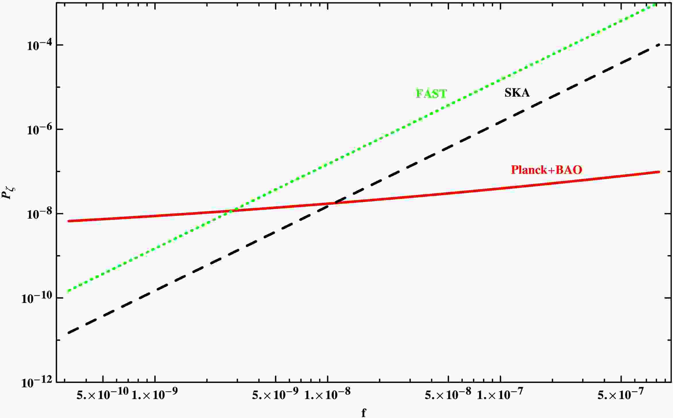
$ \Omega_{{\rm{GW}}} $ over the detectable ranges, which can be used to search for scalar-induced gravitational waves. For a comprehensive forecast, we consider two scenarios at a given frequency: one in which gravitational-wave detectors do not detect scalar-induced gravitational waves, thereby placing an upper limit on the fractional energy density; and another in which they do detect them, thereby placing a lower limit. Combining these limits with Eq. (17), we derive constraints on the power spectrum of primordial curvature perturbations. In comparison with the LIGO, Virgo, LISA, and PTA detectors, the FAST sensitivity curve intersects the scalar-induced gravitational-wave energy-density spectrum$ \Omega_{{\rm{GW}}} $ at$ 3\times10^{-9} $ Hz, as shown in Figure 3 of [42]. This indicates that the FAST detector reaches the region predicted by Planck+BAO observations and splits it into two parts at frequencies below$ 3\times10^{-9} $ Hz, as is also evident in Fig. 1. We plot the power-law scalar power spectrum$ {\cal{P}}_{\zeta} $ from Planck+BAO, FAST, and SKA across all scales relevant for this work and indicate where the additional constraints from FAST and SKA arise. The region above the dashed green curve represents the lower-limit region for FAST, and the region below the dashed green curve represents the upper-limit region. According to the sensitivity curve of FAST [12], these bounds should be achievable.
Figure 1. (color online) The power-law scalar power spectrum
$ {\cal{P}}_{\zeta} $ , as constrained by Planck+BAO, FAST, and SKA, is shown across all scales.$ \begin{aligned} \Omega_{{\rm{GW}}}&=\frac{2\pi^2}{3H_0^2}f^2h_c^2(f),\quad h_c(f)=1.5\times10^{-17}\times\frac{f}{3.17\times10^{-8}}, \end{aligned} $
(18) The fractional energy density of scalar-induced gravitational waves at a frequency of
$ 6.34\times10^{-10} $ Hz is of order$ 10^{-19} $ . Accordingly, at$ 6.34\times10^{-10} $ Hz we adopt an upper limit$ \Omega_{{\rm{GW}}}<10^{-19} $ and a lower limit$ \Omega_{{\rm{GW}}}>10^{-19} $ , which will be used in the following section. Similarly, for SKA,$ \begin{aligned} \Omega_{{\rm{GW}}}&=\frac{2\pi^2}{3H_0^2}f^2h_c^2(f),\quad h_c(f)=1.5\times10^{-18}\times\frac{f}{3.17\times10^{-8}}, \end{aligned} $
(19) The upper limit is
$ \Omega_{{\rm{GW}}}<10^{-22} $ , and the lower limit is$ \Omega_{{\rm{GW}}}>10^{-22} $ at a frequency of$ 3.17\times10^{-10} $ Hz. The values of$ \Omega_{{\rm{GW}}} $ adopted for FAST and SKA are obtained from the corresponding sensitivity curves. Through Eq. (17), the fractional energy density$ \Omega_{{\rm{GW}}} $ is related to the parameters of the power-law spectrum. Since the spectral parameters$ \{A_s, n_s, \alpha_s, \beta_s\} $ influence the fractional energy density, they are sensitive to the upper or lower limits derived from FAST. We therefore expect that the FAST sensitivity curve will yield distinct constraints on the power-law spectral parameters. For FAST and SKA, the accessible frequency range extends down to the sub-nanohertz regime, where the fractional energy density changes markedly. It is therefore anticipated that measurements in this regime will yield characteristically distinct limits on the spectral-index parameters.Recently, the PTA community has achieved significant progress, with multiple collaborations presenting compelling evidence supporting the existence of a stochastic signal in the frequency range of approximately 1–100 nHz. The presence of the currently observed foreground will greatly limit the constraining power of future observations on the subdominant stochastic gravitational-wave background [61]. For FAST and SKA, the observation span is assumed to be 50 years and 100 years, respectively [12]. The accessible frequency range extends below nHz. In this work, we consider upper and lower limits at frequencies below nHz, where no observations are yet available. Currently, we can neglect the impact of possible foregrounds at frequencies below nHz. It will be necessary to account for foreground noise in the future, once observations at frequencies below nHz become available and we search for a subdominant stochastic gravitational-wave background. In the future, when PTA observations are able to detect stochastic signals in the sub-nHz band, a measured energy density significantly higher than
$ 10^{-17} $ could be attributed to non-SIGW origins, as is currently done for existing signals; this aligns with the predictions of this work. If the detected energy density is comparable to the predicted SIGW level, the signal might originate from scalar-induced gravitational waves, a hypothesis that could be tested using the scalar spectral index as a distinguishing indicator. Given that multiple source populations likely contribute to the stochastic background, removing the brighter astrophysical foreground components may reveal a residual compatible with SIGWs. As detector sensitivities improve, a clear SIGW signature is expected to emerge in future data, underscoring the importance of monitoring$ n_s $ as a key diagnostic in separating cosmological from astrophysical gravitational-wave backgrounds. -
In the conformal Newtonian gauge, the metric perturbations of the Friedmann-Robertson-Walker (FRW) background are typically written as
$ {\rm{d}}s^2=a^2\left\{-(1+2\Phi){\rm{d}}\eta^2+\left[(1-2\Phi)\delta_{ij}+\frac{h_{ij}}{2}\right]{\rm{d}}x^i{\rm{d}}x^j \right\}, $
(1) where η denotes conformal time,
$ a(\eta) $ is the scale factor of the FRW universe, Φ is the scalar perturbation representing the gravitational potential, and$ h_{ij} $ denotes the tensor perturbation, which is transverse and traceless. We neglect vector perturbations, first-order gravitational waves, and anisotropic stress. In Fourier space, the tensor perturbation$ h_{ij} $ is expressed as$ h_{ij}(\eta,{\bf{x}})=\int\frac{{\rm{d}}^3k}{(2\pi)^{3/2}}\Bigg(e_{ij}^+({\bf{k}})h_{{\bf{k}}}^+(\eta)+e_{ij}^\times({\bf{k}})h_{{\bf{k}}}^\times(\eta)\Bigg)e^{i{\bf{k}}\cdot{\bf{x}}}, $
(2) where the plus and cross polarization tensors are
$\begin{aligned}[b]& e_{ij}^+({\bf{k}})=\frac{1}{\sqrt{2}}\Bigg(e_i({\bf{k}})e_j({\bf{k}})-\bar{e}_i({\bf{k}})\bar{e}_j({\bf{k}})\Bigg),\\& e_{ij}^\times({\bf{k}})=\frac{1}{\sqrt{2}}\Bigg(e_i({\bf{k}})\bar{e}_j({\bf{k}})+\bar{e}_i({\bf{k}})e_j({\bf{k}})\Bigg),\end{aligned} $
(3) The normalized vectors
$ e_i({\bf{k}}) $ and$ \bar{e}_i({\bf{k}}) $ are mutually orthogonal and transverse to$ {\bf{k}} $ . The tensor equation of motion for$ h_{ij} $ can be straightforwardly derived from the perturbed Einstein equations up to second order. Scalar perturbations couple to tensor perturbations in the second-order equation. Within the framework of an FRW universe, we also consider the propagation speed of scalar-induced gravitational waves and assume this speed to be a constant parameter. The equation governing induced gravitational waves, with a source term constructed from$ \Phi_{{\bf{k}}} $ , is given by$ h_{{\bf{k}}}^{"}(\eta)+2{\cal{H}}h_{{\bf{k}}}^{'}(\eta)+c_g^2k^2h_{{\bf{k}}}(\eta)=4S_{{\bf{k}}}(\eta), $
(4) where the prime denotes a derivative with respect to conformal time,
$ {\cal{H}}=a^{'}/a=aH $ represents the conformal Hubble parameter, and$ c_g $ denotes the speed of scalar-induced gravitational waves. In this paper,$ c_g $ is treated as a phenomenological parameterization of the propagation speed, rather than being embedded within a fully specified theoretical framework. The source term is given by$\begin{aligned}[b] S_{{\bf{k}}}=\;&\int\frac{{\rm{d}}^3q}{(2\pi)^{3/2}}e_{ij}({\bf{k}})q_iq_j\Bigg(2\Phi_{{\bf{q}}}\Phi_{{{\bf{k}}-{\bf{q}}}}\\&+\frac{4}{3(1+\omega)}\left({\cal{H}}^{-1}\Phi^{\prime}_{{\bf{q}}}+\Phi_{{\bf{q}}}\right)\left({\cal{H}}^{-1}\Phi^{\prime}_{{{\bf{k}}-{\bf{q}}}}+\Phi_{{{\bf{k}}-{\bf{q}}}}\right)\Bigg).\end{aligned} $
(5) We employ the Green's function method:
$ h_{{\bf{k}}}(\eta)=\frac{4}{a(\eta)}\int^{\eta}{{\rm{d}}}\bar{\eta}G_{{\bf{k}}}(\eta,\bar{\eta})a(\bar{\eta})S_{{\bf{k}}}(\bar{\eta}), $
(6) where
$ G_{{\bf{k}}}(\eta,\bar{\eta}) $ satisfies the equation$ G_{{\bf{k}}}^{"}(\eta,\bar{\eta})+\left(c_g^2k^2-\frac{a^{"}(\eta)}{a(\eta)}\right)G_{{\bf{k}}}(\eta,\bar{\eta})=\delta(\eta-\bar{\eta}). $
(7) In the radiation-dominated Universe, the Green's function solution is
$ G_{{\bf{k}}}(\eta,\bar{\eta})=\frac{1}{c_gk}\sin[c_gk(\eta-\bar{\eta})]\Theta(\eta-\bar{\eta}), $
(8) where Θ is the Heaviside step function.
The power spectrum of scalar-induced gravitational waves is defined as
$ \langle h_{{\bf{k}}}(\eta) h_{{\bf{k}}^{\prime}}(\eta)\rangle=\frac{2\pi^2}{k^3}\delta^{(3)}({\bf{k}}+{\bf{k}}^{\prime}){\cal{P}}_h(\eta, k), $
(9) and the fractional energy density is defined as [59, 60]
$ \Omega_{{\rm{GW}}}(\eta, k)=\frac{1}{\rho_c}\frac{d\rho_{{\rm{GW}}}}{d\ln k}=\frac{1}{24}\Bigg(\frac{c_gk}{aH}\Bigg)^2\overline{{\cal{P}}_h(\eta, k)}, $
(10) where
$ \rho_{{\rm{GW}}} $ is the energy density of the stochastic gravitational-wave background, and$ \rho_c $ is the critical energy density. After calculation, the power spectrum of scalar-induced gravitational waves takes the form$\begin{aligned}[b] {\cal{P}}_h(\eta, k)=\;&4\int_0^\infty{\rm{d}}v\int_{\vert1-v\vert}^{1+v}{\rm{d}}u\left(\frac{4v^2-(1+v^2-u^2)^2}{4vu}\right)^2\\&\times I^2(v, u, x){\cal{P}}_{\zeta}(kv){\cal{P}}_{\zeta}(ku),\end{aligned} $
(11) where
$ {\cal{P}}_{\zeta}(k) $ is the power spectrum of primordial curvature perturbations,$ x\equiv k\eta $ ,$ u=|{\bf{k}}-\tilde{{\bf{k}}}|/k $ , and$ v=\tilde{k}/k $ . The function$ I(v, u, x) $ is defined by$ I(v, u, x)=\int_0^x{\rm{d}}\bar{x}\frac{a(\bar{\eta})}{a(\eta)}kG_{{\bf{k}}}(\eta, \bar{\eta})f(v, u, \bar{x}), $
(12) where
$ \bar{x}\equiv k\bar{\eta} $ and$ f(v, u, \bar{x}) $ arises from the source term.$ \begin{aligned}[b] f(v, u, \bar{x})=\;&\frac{6(\omega+1)}{3\omega+5}\Phi(v\bar x)\Phi(u\bar x)+\frac{6(1+3\omega)(\omega+1)}{(3\omega+5)^2}\\&\times\Big(\bar x \partial_{\bar{\eta}}\Phi(v\bar x)\Phi(u\bar x)+\bar x \partial_{\bar{\eta}}\Phi(u\bar x)\Phi(v\bar x)\Big) \\ &+\frac{3(1+3\omega)^2(1+\omega)}{(3\omega+5)^2}{\bar x}^2\partial_{\bar{\eta}}\Phi(v\bar x)\partial_{\bar{\eta}}\Phi(u\bar x). \end{aligned} $
(13) In a radiation-dominated universe, the functions
$ f(v, u, \bar{x}) $ and$ I(v, u, x) $ are given in our previous study [50].For a power-law scalar power spectrum, we have
$ \begin{aligned} {\cal{P}}_{\zeta}(k)&=A_s\left(\frac{k}{k_*}\right)^{n_s-1+\frac{1}{2}\alpha_s\ln(k/k_*)+\frac{1}{6}\beta_s(\ln(k/k_*))^2}, \end{aligned} $
(14) The power spectrum of scalar-induced gravitational waves is given by Ref. [50]:
$ \begin{aligned}[b]{\cal{P}}_h(\eta, k)=\;&\frac{24Q(c_g, n_s, \alpha_s, \beta_s, k)}{(k\eta)^2}A^2_s\\&\times\left(\frac{k}{k_*}\right)^{2 \left[ {n_s-1+\frac{1}{2}\alpha_s\ln(k/k_*)+\frac{1}{6}\beta_s(\ln(k/k_*))^2}\right]},\end{aligned} $
(15) where
$ A_s $ denotes the scalar amplitude of the power-law power spectrum at the pivot scale$ k_*=0.05 $ Mpc$ ^{-1} $ ,$ n_s $ is the scalar spectral index,$ \alpha_s\equiv{\rm{d}} n_s/{\rm{d}}\ln k $ is the running of the scalar spectral index,$ \beta_s\equiv{{\rm{d}}^2n_s}/{{\rm{d}}\ln k^2} $ is the running of the running of the scalar spectral index, and$ Q(c_g, n_s, \alpha_s, \beta_s, k) $ denotes the overall coefficients.$ \begin{aligned}[b] Q(c_g, n_s, \alpha_s, \beta_s, k)=&\frac{1}{12}\int_0^\infty{\rm{d}}v\int_{\vert1-v\vert}^{1+v}{\rm{d}}u \Bigg(\frac{4v^2-(1+v^2-u^2)^2}{4vu}\Bigg)^2 \Bigg(\frac{3(u^2+v^2-3c_g^2)}{4u^3v^3}\Bigg)^2 \\ &\Bigg(\Big(-4uv+(u^2+v^2-3c_g^2)\log\left|\frac{3c_g^2-(u+v)^2}{3c_g^2-(u-v)^2}\right|\Big)^2+\pi^2(u^2+v^2-3c_g^2)^2\Theta(u+v-\sqrt{3}c_g)\Bigg) \\ &\Bigg(\frac{k}{k_*}\Bigg)^{\frac{1}{2}\alpha_s\ln(uv)+\frac{1}{6}\beta_s\Big((\ln{v})^2+2\ln{v}\ln(k/k_*)+(\ln{u})^2+2\ln{u}\ln(k/k_*)\Big)}\Bigg(uv\Bigg)^{n_s-1+\frac{1}{2}\alpha_s\ln(k/k_*)+\frac{1}{6}\beta_s(\ln(k/k_*))^2}\\ &v^{\frac{1}{2}\alpha_s\ln{v}+\frac{1}{6}\beta_s\Big((\ln{v})^2+2\ln{v}\ln(k/k_*)\Big)}u^{\frac{1}{2}\alpha_s\ln{u}+\frac{1}{6}\beta_s\Big((\ln{u})^2+2\ln{u}\ln(k/k_*)\Big)}, \end{aligned} $
(16) This quantity is the integral over u and v and depends on
$ c_g $ ,$ n_s $ ,$ \alpha_s $ ,$ \beta_s $ , and k. Numerical values for representative parameter sets are listed in Table 4 of [50]. The connection between the parameters of the power-law spectrum and scalar-induced gravitational waves has been established. The fractional energy density is${ \Omega_{{\rm{GW}}}(\eta, k)=Q(c_g, n_s, \alpha_s, \beta_s, k)A^2_s\left(\dfrac{k}{k_*}\right)^{2 \left[{n_s-1+\frac{1}{2}\alpha_s\ln(k/k_*)+\frac{1}{6}\beta_s(\ln(k/k_*))^2}\right]}.} $
(17) Here, we first investigate scalar-induced gravitational waves that propagate at the speed of light. According to Planck+BAO observations [53], the central values are
$ n_s=0.9647\pm0.0043 $ ,$ \alpha_s=0.009\pm0.012 $ , and$ \beta_s=0.0011\pm0.0099 $ . Although Planck+BAO data do not directly probe frequencies in the nHz range, we assume that the curvature power spectrum can be extrapolated from the CMB to PTA scales without significant running. The fractional energy density of scalar-induced gravitational waves at a frequency of$ 10^{-10} $ Hz is expected to be of order$ 10^{-17} $ .Gravitational-wave detections also provide sensitivity curves in frequency and
$ \Omega_{{\rm{GW}}} $ over the detectable ranges, which can be used to search for scalar-induced gravitational waves. For a comprehensive forecast, we consider two scenarios at a given frequency: one in which gravitational-wave detectors do not detect scalar-induced gravitational waves, thereby placing an upper limit on the fractional energy density; and another in which they do detect them, thereby placing a lower limit. Combining these limits with Eq. (17), we derive constraints on the power spectrum of primordial curvature perturbations. In comparison with the LIGO, Virgo, LISA, and PTA detectors, the FAST sensitivity curve intersects the scalar-induced gravitational-wave energy-density spectrum$ \Omega_{{\rm{GW}}} $ at$ 3\times10^{-9} $ Hz, as shown in Figure 3 of [42]. This indicates that the FAST detector reaches the region predicted by Planck+BAO observations and splits it into two parts at frequencies below$ 3\times10^{-9} $ Hz, as is also evident in Figure 1. We plot the power-law scalar power spectrum$ {\cal{P}}_{\zeta} $ from Planck+BAO, FAST, and SKA across all scales relevant for this work and indicate where the additional constraints from FAST and SKA arise. The region above the dashed green curve represents the lower-limit region for FAST, and the region below the dashed green curve represents the upper-limit region. According to the sensitivity curve of FAST [12], these bounds should be achievable.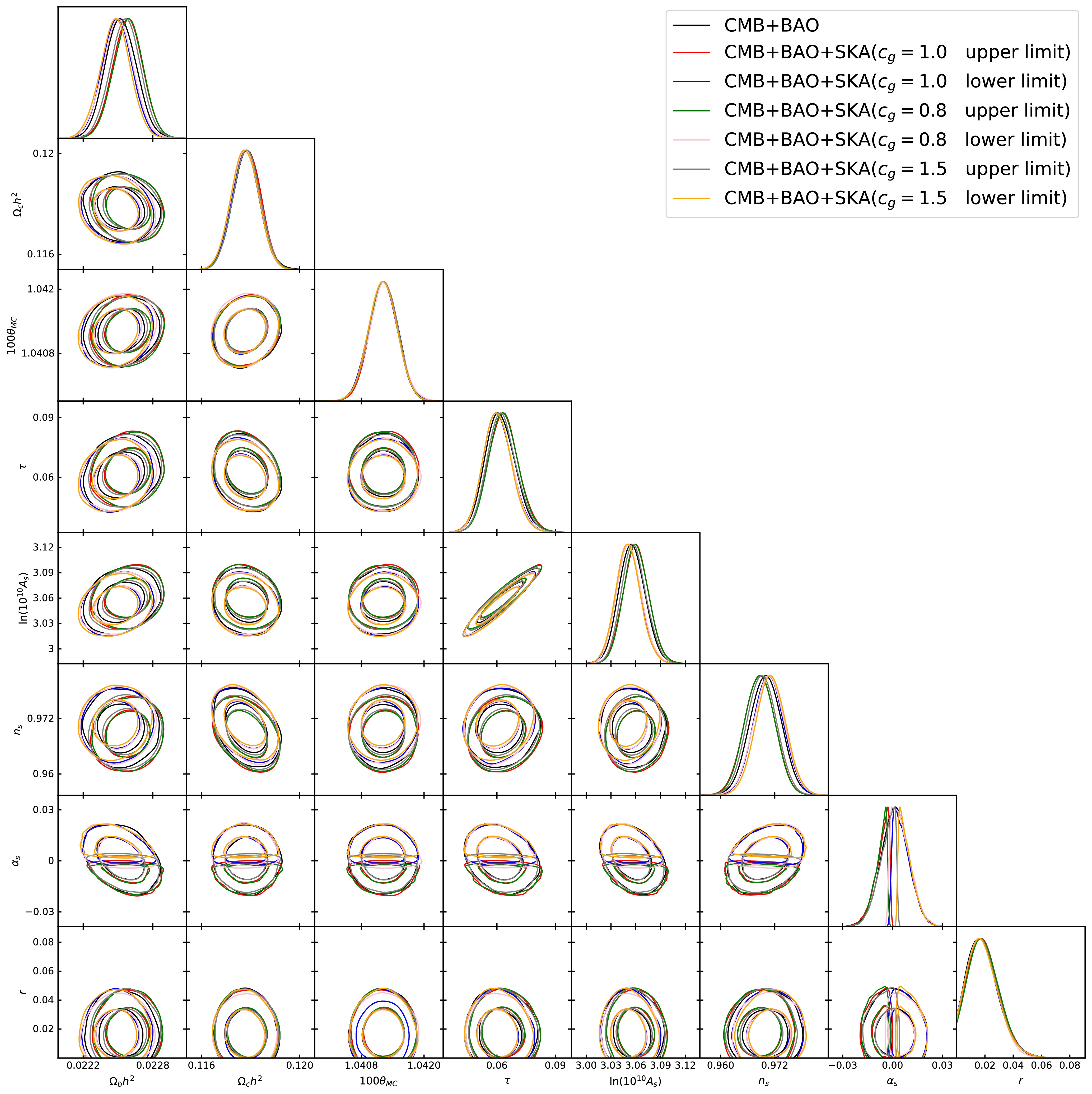
Figure 3. The contour plots and likelihood distributions of cosmological parameters in the ΛCDM+
$ \alpha_s $ +r model are shown at the 68% and 95% confidence levels, derived from the combinations CMB+BAO, CMB+BAO+SKA($ c_g=1.0$ upper limit), CMB+BAO+SKA($ c_g=1.0$ lower limit), CMB+BAO+SKA($ c_g=0.8$ upper limit), CMB+BAO+SKA($ c_g=0.8$ lower limit), CMB+BAO+SKA($ c_g=1.5$ upper limit), and CMB+BAO+SKA($ c_g=1.5$ lower limit). The solid lines in the likelihood distributions represent the constraints from the CMB+BAO+SKA datasets. The dashed lines in the likelihood distributions represent the constraints from the CMB+BAO dataset.
Figure 1. (color online) The power-law scalar power spectrum
$ {\cal{P}}_{\zeta} $ , as constrained by Planck+BAO, FAST, and SKA, is shown across all scales.$ \begin{aligned} \Omega_{{\rm{GW}}}&=\frac{2\pi^2}{3H_0^2}f^2h_c^2(f),\quad h_c(f)=1.5\times10^{-17}\times\frac{f}{3.17\times10^{-8}}, \end{aligned} $
(18) The fractional energy density of scalar-induced gravitational waves at a frequency of
$ 6.34\times10^{-10} $ Hz is of order$ 10^{-19} $ . Accordingly, at$ 6.34\times10^{-10} $ Hz we adopt an upper limit$ \Omega_{{\rm{GW}}}<10^{-19} $ and a lower limit$ \Omega_{{\rm{GW}}}>10^{-19} $ , which will be used in the following section. Similarly, for SKA,$ \begin{aligned} \Omega_{{\rm{GW}}}&=\frac{2\pi^2}{3H_0^2}f^2h_c^2(f),\quad h_c(f)=1.5\times10^{-18}\times\frac{f}{3.17\times10^{-8}}, \end{aligned} $
(19) The upper limit is
$ \Omega_{{\rm{GW}}}<10^{-22} $ , and the lower limit is$ \Omega_{{\rm{GW}}}>10^{-22} $ at a frequency of$ 3.17\times10^{-10} $ Hz. The values of$ \Omega_{{\rm{GW}}} $ adopted for FAST and SKA are obtained from the corresponding sensitivity curves. Through Eq. (17), the fractional energy density$ \Omega_{{\rm{GW}}} $ is related to the parameters of the power-law spectrum. Since the spectral parameters$ \{A_s, n_s, \alpha_s, \beta_s\} $ influence the fractional energy density, they are sensitive to the upper or lower limits derived from FAST. We therefore expect that the FAST sensitivity curve will yield distinct constraints on the power-law spectral parameters. For FAST and SKA, the accessible frequency range extends down to the sub-nanohertz regime, where the fractional energy density changes markedly. It is therefore anticipated that measurements in this regime will yield characteristically distinct limits on the spectral-index parameters.Recently, the PTA community has achieved significant progress, with multiple collaborations presenting compelling evidence supporting the existence of a stochastic signal in the frequency range of approximately 1–100 nHz. The presence of the currently observed foreground will greatly limit the constraining power of future observations on the subdominant stochastic gravitational-wave background [61]. For FAST and SKA, the observation span is assumed to be 50 years and 100 years, respectively [12]. The accessible frequency range extends below nHz. In this work, we consider upper and lower limits at frequencies below nHz, where no observations are yet available. Currently, we can neglect the impact of possible foregrounds at frequencies below nHz. It will be necessary to account for foreground noise in the future, once observations at frequencies below nHz become available and we search for a subdominant stochastic gravitational-wave background. In the future, when PTA observations are able to detect stochastic signals in the sub-nHz band, a measured energy density significantly higher than
$ 10^{-17} $ could be attributed to non-SIGW origins, as is currently done for existing signals; this aligns with the predictions of this work. If the detected energy density is comparable to the predicted SIGW level, the signal might originate from scalar-induced gravitational waves, a hypothesis that could be tested using the scalar spectral index as a distinguishing indicator. Given that multiple source populations likely contribute to the stochastic background, removing the brighter astrophysical foreground components may reveal a residual compatible with SIGWs. As detector sensitivities improve, a clear SIGW signature is expected to emerge in future data, underscoring the importance of monitoring$ n_s $ as a key diagnostic in separating cosmological from astrophysical gravitational-wave backgrounds. -
In the conformal Newtonian gauge, the metric perturbations of the Friedmann-Robertson-Walker (FRW) background are typically written as
$ {\rm{d}}s^2=a^2\left\{-(1+2\Phi){\rm{d}}\eta^2+\left[(1-2\Phi)\delta_{ij}+\frac{h_{ij}}{2}\right]{\rm{d}}x^i{\rm{d}}x^j \right\}, $
(1) where η denotes conformal time,
$ a(\eta) $ is the scale factor of the FRW universe, Φ is the scalar perturbation representing the gravitational potential, and$ h_{ij} $ denotes the tensor perturbation, which is transverse and traceless. We neglect vector perturbations, first-order gravitational waves, and anisotropic stress. In Fourier space, the tensor perturbation$ h_{ij} $ is expressed as$ h_{ij}(\eta,{\bf{x}})=\int\frac{{\rm{d}}^3k}{(2\pi)^{3/2}}\Bigg(e_{ij}^+({\bf{k}})h_{{\bf{k}}}^+(\eta)+e_{ij}^\times({\bf{k}})h_{{\bf{k}}}^\times(\eta)\Bigg) {\rm e}^{{\rm i}{\bf{k}}\cdot{\bf{x}}}, $
(2) where the plus and cross polarization tensors are
$\begin{aligned}[b]& e_{ij}^+({\bf{k}})=\frac{1}{\sqrt{2}}\Bigg(e_i({\bf{k}})e_j({\bf{k}})-\bar{e}_i({\bf{k}})\bar{e}_j({\bf{k}})\Bigg),\\& e_{ij}^\times({\bf{k}})=\frac{1}{\sqrt{2}}\Bigg(e_i({\bf{k}})\bar{e}_j({\bf{k}})+\bar{e}_i({\bf{k}})e_j({\bf{k}})\Bigg),\end{aligned} $
(3) The normalized vectors
$ e_i({\bf{k}}) $ and$ \bar{e}_i({\bf{k}}) $ are mutually orthogonal and transverse to$ {\bf{k}} $ . The tensor equation of motion for$ h_{ij} $ can be straightforwardly derived from the perturbed Einstein equations up to second order. Scalar perturbations couple to tensor perturbations in the second-order equation. Within the framework of an FRW universe, we also consider the propagation speed of scalar-induced gravitational waves and assume this speed to be a constant parameter. The equation governing induced gravitational waves, with a source term constructed from$ \Phi_{{\bf{k}}} $ , is given by$ h_{{\bf{k}}}^{"}(\eta)+2{\cal{H}}h_{{\bf{k}}}^{'}(\eta)+c_g^2k^2h_{{\bf{k}}}(\eta)=4S_{{\bf{k}}}(\eta), $
(4) where the prime denotes a derivative with respect to conformal time,
$ {\cal{H}}=a'/a=aH $ represents the conformal Hubble parameter, and$ c_g $ denotes the speed of scalar-induced gravitational waves. In this paper,$ c_g $ is treated as a phenomenological parameterization of the propagation speed, rather than being embedded within a fully specified theoretical framework. The source term is given by$\begin{aligned}[b] S_{{\bf{k}}}=\;&\int\frac{{\rm{d}}^3q}{(2\pi)^{3/2}}e_{ij}({\bf{k}})q_iq_j\Bigg(2\Phi_{{\bf{q}}}\Phi_{{{\bf{k}}-{\bf{q}}}}\\&+\frac{4}{3(1+\omega)}\left({\cal{H}}^{-1}\Phi^{\prime}_{{\bf{q}}}+\Phi_{{\bf{q}}}\right)\left({\cal{H}}^{-1}\Phi^{\prime}_{{{\bf{k}}-{\bf{q}}}}+\Phi_{{{\bf{k}}-{\bf{q}}}}\right)\Bigg).\end{aligned} $
(5) We employ the Green's function method:
$ h_{{\bf{k}}}(\eta)=\frac{4}{a(\eta)}\int^{\eta}{{\rm{d}}}\bar{\eta}G_{{\bf{k}}}(\eta,\bar{\eta})a(\bar{\eta})S_{{\bf{k}}}(\bar{\eta}), $
(6) where
$ G_{{\bf{k}}}(\eta,\bar{\eta}) $ satisfies the equation$ G_{{\bf{k}}}''(\eta,\bar{\eta})+\left(c_g^2k^2-\frac{a''(\eta)}{a(\eta)}\right)G_{{\bf{k}}}(\eta,\bar{\eta})=\delta(\eta-\bar{\eta}). $
(7) In the radiation-dominated Universe, the Green's function solution is
$ G_{{\bf{k}}}(\eta,\bar{\eta})=\frac{1}{c_gk}\sin[c_gk(\eta-\bar{\eta})]\Theta(\eta-\bar{\eta}), $
(8) where Θ is the Heaviside step function.
The power spectrum of scalar-induced gravitational waves is defined as
$ \langle h_{{\bf{k}}}(\eta) h_{{\bf{k}}^{\prime}}(\eta)\rangle=\frac{2\pi^2}{k^3}\delta^{(3)}({\bf{k}}+{\bf{k}}^{\prime}){\cal{P}}_h(\eta, k), $
(9) and the fractional energy density is defined as [59, 60]
$ \Omega_{{\rm{GW}}}(\eta, k)=\frac{1}{\rho_c}\frac{{\rm d} \rho_{{\rm{GW}}}}{{\rm d}\ln k}=\frac{1}{24}\Bigg(\frac{c_gk}{aH}\Bigg)^2\overline{{\cal{P}}_h(\eta, k)}, $
(10) where
$ \rho_{{\rm{GW}}} $ is the energy density of the stochastic gravitational-wave background, and$ \rho_c $ is the critical energy density. After calculation, the power spectrum of scalar-induced gravitational waves takes the form$\begin{aligned}[b] {\cal{P}}_h(\eta, k)=\;&4\int_0^\infty{\rm{d}}v\int_{\vert1-v\vert}^{1+v}{\rm{d}}u\left(\frac{4v^2-(1+v^2-u^2)^2}{4vu}\right)^2\\&\times I^2(v, u, x){\cal{P}}_{\zeta}(kv){\cal{P}}_{\zeta}(ku),\end{aligned} $
(11) where
$ {\cal{P}}_{\zeta}(k) $ is the power spectrum of primordial curvature perturbations,$ x\equiv k\eta $ ,$ u=|{\bf{k}}-\tilde{{\bf{k}}}|/k $ , and$ v=\tilde{k}/k $ . The function$ I(v, u, x) $ is defined by$ I(v, u, x)=\int_0^x{\rm{d}}\bar{x}\frac{a(\bar{\eta})}{a(\eta)}kG_{{\bf{k}}}(\eta, \bar{\eta})f(v, u, \bar{x}), $
(12) where
$ \bar{x}\equiv k\bar{\eta} $ and$ f(v, u, \bar{x}) $ arises from the source term.$ \begin{aligned}[b] f(v, u, \bar{x})=\;&\frac{6(\omega+1)}{3\omega+5}\Phi(v\bar x)\Phi(u\bar x)+\frac{6(1+3\omega)(\omega+1)}{(3\omega+5)^2}\\&\times\Big(\bar x \partial_{\bar{\eta}}\Phi(v\bar x)\Phi(u\bar x)+\bar x \partial_{\bar{\eta}}\Phi(u\bar x)\Phi(v\bar x)\Big) \\ &+\frac{3(1+3\omega)^2(1+\omega)}{(3\omega+5)^2}{\bar x}^2\partial_{\bar{\eta}}\Phi(v\bar x)\partial_{\bar{\eta}}\Phi(u\bar x). \end{aligned} $
(13) In a radiation-dominated universe, the functions
$ f(v, u, \bar{x}) $ and$ I(v, u, x) $ are given in our previous study [50].For a power-law scalar power spectrum, we have
$ \begin{aligned} {\cal{P}}_{\zeta}(k)&=A_s\left(\frac{k}{k_*}\right)^{n_s-1+\frac{1}{2}\alpha_s\ln(k/k_*)+\frac{1}{6}\beta_s(\ln(k/k_*))^2}, \end{aligned} $
(14) The power spectrum of scalar-induced gravitational waves is given by Ref. [50]:
$ \begin{aligned}[b]{\cal{P}}_h(\eta, k)=\;&\frac{24Q(c_g, n_s, \alpha_s, \beta_s, k)}{(k\eta)^2}A^2_s\\&\times\left(\frac{k}{k_*}\right)^{2 \left[ {n_s-1+\frac{1}{2}\alpha_s\ln(k/k_*)+\frac{1}{6}\beta_s(\ln(k/k_*))^2}\right]},\end{aligned} $
(15) where
$ A_s $ denotes the scalar amplitude of the power-law power spectrum at the pivot scale$ k_*=0.05 $ Mpc$ ^{-1} $ ,$ n_s $ is the scalar spectral index,$ \alpha_s\equiv{\rm{d}} n_s/{\rm{d}}\ln k $ is the running of the scalar spectral index,$ \beta_s\equiv{{\rm{d}}^2n_s}/{{\rm{d}}\ln k^2} $ is the running of the running of the scalar spectral index, and$ Q(c_g, n_s, \alpha_s, \beta_s, k) $ denotes the overall coefficients.$ \begin{aligned}[b] Q(c_g, n_s, \alpha_s, \beta_s, k)=&\frac{1}{12}\int_0^\infty{\rm{d}}v\int_{\vert1-v\vert}^{1+v}{\rm{d}}u \Bigg(\frac{4v^2-(1+v^2-u^2)^2}{4vu}\Bigg)^2 \Bigg(\frac{3(u^2+v^2-3c_g^2)}{4u^3v^3}\Bigg)^2 \\ & \times \Bigg(\Big(-4uv+(u^2+v^2-3c_g^2)\log\left|\frac{3c_g^2-(u+v)^2}{3c_g^2-(u-v)^2}\right|\Big)^2+\pi^2(u^2+v^2-3c_g^2)^2\Theta(u+v-\sqrt{3}c_g)\Bigg) \\ & \times \Bigg(\frac{k}{k_*}\Bigg)^{\frac{1}{2}\alpha_s\ln(uv)+\frac{1}{6}\beta_s\Big((\ln{v})^2+2\ln{v}\ln(k/k_*)+(\ln{u})^2+2\ln{u}\ln(k/k_*)\Big)}\Bigg(uv\Bigg)^{n_s-1+\frac{1}{2}\alpha_s\ln(k/k_*)+\frac{1}{6}\beta_s(\ln(k/k_*))^2}\\ & \times v^{\frac{1}{2}\alpha_s\ln{v}+\frac{1}{6}\beta_s\Big((\ln{v})^2+2\ln{v}\ln(k/k_*)\Big)}u^{\frac{1}{2}\alpha_s\ln{u}+\frac{1}{6}\beta_s\Big((\ln{u})^2+2\ln{u}\ln(k/k_*)\Big)}, \end{aligned} $
(16) This quantity is the integral over u and v and depends on
$ c_g $ ,$ n_s $ ,$ \alpha_s $ ,$ \beta_s $ , and k. Numerical values for representative parameter sets are listed in Table 4 of [50]. The connection between the parameters of the power-law spectrum and scalar-induced gravitational waves has been established. The fractional energy density is${ \Omega_{{\rm{GW}}}(\eta, k)=Q(c_g, n_s, \alpha_s, \beta_s, k)A^2_s\left(\dfrac{k}{k_*}\right)^{2 \left[{n_s-1+\frac{1}{2}\alpha_s\ln(k/k_*)+\frac{1}{6}\beta_s(\ln(k/k_*))^2}\right]}.} $
(17) Here, we first investigate scalar-induced gravitational waves that propagate at the speed of light. According to Planck+BAO observations [53], the central values are
$ n_s=0.9647\pm0.0043 $ ,$ \alpha_s=0.009\pm0.012 $ , and$ \beta_s=0.0011\pm 0.0099 $ . Although Planck+BAO data do not directly probe frequencies in the nHz range, we assume that the curvature power spectrum can be extrapolated from the CMB to PTA scales without significant running. The fractional energy density of scalar-induced gravitational waves at a frequency of$ 10^{-10} $ Hz is expected to be of order$ 10^{-17} $ .Gravitational-wave detections also provide sensitivity curves in frequency and
$ \Omega_{{\rm{GW}}} $ over the detectable ranges, which can be used to search for scalar-induced gravitational waves. For a comprehensive forecast, we consider two scenarios at a given frequency: one in which gravitational-wave detectors do not detect scalar-induced gravitational waves, thereby placing an upper limit on the fractional energy density; and another in which they do detect them, thereby placing a lower limit. Combining these limits with Eq. (17), we derive constraints on the power spectrum of primordial curvature perturbations. In comparison with the LIGO, Virgo, LISA, and PTA detectors, the FAST sensitivity curve intersects the scalar-induced gravitational-wave energy-density spectrum$ \Omega_{{\rm{GW}}} $ at$ 3\times10^{-9} $ Hz, as shown in Figure 3 of [42]. This indicates that the FAST detector reaches the region predicted by Planck+BAO observations and splits it into two parts at frequencies below$ 3\times10^{-9} $ Hz, as is also evident in Fig. 1. We plot the power-law scalar power spectrum$ {\cal{P}}_{\zeta} $ from Planck+BAO, FAST, and SKA across all scales relevant for this work and indicate where the additional constraints from FAST and SKA arise. The region above the dashed green curve represents the lower-limit region for FAST, and the region below the dashed green curve represents the upper-limit region. According to the sensitivity curve of FAST [12], these bounds should be achievable.
Figure 1. (color online) The power-law scalar power spectrum
$ {\cal{P}}_{\zeta} $ , as constrained by Planck+BAO, FAST, and SKA, is shown across all scales.$ \begin{aligned} \Omega_{{\rm{GW}}}&=\frac{2\pi^2}{3H_0^2}f^2h_c^2(f),\quad h_c(f)=1.5\times10^{-17}\times\frac{f}{3.17\times10^{-8}}, \end{aligned} $
(18) The fractional energy density of scalar-induced gravitational waves at a frequency of
$ 6.34\times10^{-10} $ Hz is of order$ 10^{-19} $ . Accordingly, at$ 6.34\times10^{-10} $ Hz we adopt an upper limit$ \Omega_{{\rm{GW}}}<10^{-19} $ and a lower limit$ \Omega_{{\rm{GW}}}>10^{-19} $ , which will be used in the following section. Similarly, for SKA,$ \begin{aligned} \Omega_{{\rm{GW}}}&=\frac{2\pi^2}{3H_0^2}f^2h_c^2(f),\quad h_c(f)=1.5\times10^{-18}\times\frac{f}{3.17\times10^{-8}}, \end{aligned} $
(19) The upper limit is
$ \Omega_{{\rm{GW}}}<10^{-22} $ , and the lower limit is$ \Omega_{{\rm{GW}}}>10^{-22} $ at a frequency of$ 3.17\times10^{-10} $ Hz. The values of$ \Omega_{{\rm{GW}}} $ adopted for FAST and SKA are obtained from the corresponding sensitivity curves. Through Eq. (17), the fractional energy density$ \Omega_{{\rm{GW}}} $ is related to the parameters of the power-law spectrum. Since the spectral parameters$ \{A_s, n_s, \alpha_s, \beta_s\} $ influence the fractional energy density, they are sensitive to the upper or lower limits derived from FAST. We therefore expect that the FAST sensitivity curve will yield distinct constraints on the power-law spectral parameters. For FAST and SKA, the accessible frequency range extends down to the sub-nanohertz regime, where the fractional energy density changes markedly. It is therefore anticipated that measurements in this regime will yield characteristically distinct limits on the spectral-index parameters.Recently, the PTA community has achieved significant progress, with multiple collaborations presenting compelling evidence supporting the existence of a stochastic signal in the frequency range of approximately 1–100 nHz. The presence of the currently observed foreground will greatly limit the constraining power of future observations on the subdominant stochastic gravitational-wave background [61]. For FAST and SKA, the observation span is assumed to be 50 years and 100 years, respectively [12]. The accessible frequency range extends below nHz. In this work, we consider upper and lower limits at frequencies below nHz, where no observations are yet available. Currently, we can neglect the impact of possible foregrounds at frequencies below nHz. It will be necessary to account for foreground noise in the future, once observations at frequencies below nHz become available and we search for a subdominant stochastic gravitational-wave background. In the future, when PTA observations are able to detect stochastic signals in the sub-nHz band, a measured energy density significantly higher than
$ 10^{-17} $ could be attributed to non-SIGW origins, as is currently done for existing signals; this aligns with the predictions of this work. If the detected energy density is comparable to the predicted SIGW level, the signal might originate from scalar-induced gravitational waves, a hypothesis that could be tested using the scalar spectral index as a distinguishing indicator. Given that multiple source populations likely contribute to the stochastic background, removing the brighter astrophysical foreground components may reveal a residual compatible with SIGWs. As detector sensitivities improve, a clear SIGW signature is expected to emerge in future data, underscoring the importance of monitoring$ n_s $ as a key diagnostic in separating cosmological from astrophysical gravitational-wave backgrounds. -
In the standard ΛCDM model, the six parameters are the baryon density parameter
$ \Omega_b h^2 $ , the cold dark matter density$ \Omega_c h^2 $ , the angular size of the horizon at the last scattering surface$ \theta_{\rm{MC}} $ , the optical depth τ, the scalar amplitude$ A_s $ and the scalar spectral index$ n_s $ . In the literature, the tensor-to-scalar ratio r is utilized to quantify the tensor amplitude$ A_t $ relative to the scalar amplitude$ A_s $ at the pivot scale, namely$ r\equiv\frac{A_t}{A_s}. $
(20) We use the publicly available Cosmomc code [62] to extend the standard ΛCDM model by incorporating parameters such as the tensor-to-scalar ratio r, the running of the scalar spectral index
$ \alpha_s $ , and the running of the running of the scalar spectral index$ \beta_s $ . In the ΛCDM+r model, the priors for the seven cosmological parameters are set following the default CosmoMC configuration, while the remaining parameters are assigned the following uniform priors:$ \alpha_s\in[-0.5,0.5] $ and$ \beta_s\in[-0.5, 0.5] $ . These parameters are constrained using the combinations of CMB+BAO, along with the upper or lower limits of the stochastic gravitational wave background provided by FAST or SKA. The likelihood for the combined CMB+ BAO dataset includes Planck TTTEEE+lowE+lensing, BICEP/Keck 2018 (BK18), 6dF Galaxy Survey, MGS, SDSS DR12, and DESI Data Release 2 (DESI DR2). The upper or lower bounds for the stochastic gravitational-wave background from FAST or SKA are implemented in the subroutine SetFast within the file CosmologyParameterizations.f90 in the source directory. The upper limits on the primordial scalar amplitude$ A_s $ inferred from SKA observations at$ 3.17\times10^{-10} $ Hz are sensitive to the assumed propagation speed of gravitational waves$ c_g $ . In the ΛCDM+r framework, the limits read$ \begin{aligned} c_g&=1.0:\quad A_s<11.5\times10^{-10}\times(4.09\times10^6)^{1-n_s}, \end{aligned} $
(21) $ \begin{aligned} c_g&=0.8:\quad A_s<9.8\times10^{-10}\times(4.09\times10^6)^{1-n_s}, \end{aligned} $
(22) $ \begin{aligned} c_g&=1.5:\quad A_s<18.3\times10^{-10}\times(4.09\times10^6)^{1-n_s}. \end{aligned} $
(23) When the running of the scalar spectral index,
$ \alpha_s $ , is included (ΛCDM+$ \alpha_s $ +r), the corresponding expressions take the following form:$ \begin{aligned} c_g&=1.0:\quad A_s<11.64\times10^{-10}\times(4.09\times10^6)^{1-n_s-7.61\alpha_s}, \end{aligned} $
(24) $ \begin{aligned} c_g&=0.8:\quad A_s<9.84\times10^{-10}\times(4.09\times10^6)^{1-n_s-7.61\alpha_s}, \end{aligned} $
(25) $ \begin{aligned} c_g&=1.5:\quad A_s<18.89\times10^{-10}\times(4.09\times10^6)^{1-n_s-7.61\alpha_s}. \end{aligned} $
(26) Finally, within the extended ΛCDM+
$ \alpha_s $ +$ \beta_s $ +r model, the limits derived from the FAST data at$ 6.34\times10^{-10} $ Hz are:$ \begin{aligned} c_g&=1.0:\quad A_s<23.77\times10^{-10}\times(8.18\times10^6)^{1-n_s-7.96\alpha_s-42.23\beta_s}, \end{aligned} $
(27) $ \begin{aligned} c_g&=0.9:\quad A_s<10.61\times10^{-10}\times(8.18\times10^6)^{1-n_s-7.96\alpha_s-42.23\beta_s}, \end{aligned} $
(28) $ \begin{aligned} c_g&=1.2:\quad A_s<12.66\times10^{-10}\times(8.18\times10^6)^{1-n_s-7.96\alpha_s-42.23\beta_s}. \end{aligned} $
(29) In this analysis, SKA data are used to constrain the ΛCDM+r and ΛCDM+
$ \alpha_s $ +r models; in these parameter spaces, the inclusion of FAST data does not provide tighter constraints than those from the CMB+BAO dataset alone. For the extended ΛCDM+$ \alpha_s $ +$ \beta_s $ +r model, FAST data are used, since the corresponding SKA constraints are much stronger than those obtained from CMB+BAO data. The numerical results are presented in Tables 1−6 and Figs. 2−4.Parameter CMB+BAO+SKA CMB+BAO+SKA
($c_g=1.0$ upper limit)CMB+BAO+SKA
($c_g=1.0$ lower limit)$ \Omega_bh^2 $ $ 0.02253\pm0.00012 $ $ 0.02247\pm0.00012 $ $ 0.02253\pm0.00012 $ $ \Omega_ch^2 $ $ 0.11783\pm{0.0006} $ $ 0.11850\pm{0.0005} $ $ 0.11782\pm{0.0006} $ $ 100\theta_{{\rm{MC}}} $ $ 1.04122\pm0.00027 $ $ 1.04117\pm0.00027 $ $ 1.04123\pm0.00027 $ τ $ 0.0619^{+0.0068}_{-0.0079} $ $ 0.0527\pm0.0060 $ $ 0.0616^{+0.0069}_{-0.0081} $ $ \ln(10^{10}A_s) $ $ 3.056^{+0.014}_{-0.016} $ $ 3.039^{+0.013}_{-0.012} $ $ 3.055^{+0.014}_{-0.016} $ $ n_s $ $ 0.9698^{+0.0033}_{-0.0032} $ $ 0.9598^{+0.0013}_{-0.0009} $ $ 0.9697\pm{0.0033} $ $ r_{0.05} $ (95% CL)$<0.039 $ $<0.038 $ $<0.040 $ Table 1. The 68% confidence limits on the cosmological parameters of the ΛCDM+r model are derived from the following dataset combinations: CMB+BAO, CMB+BAO+SKA(
$ c_g=1.0$ upper limit), and CMB+BAO+SKA($ c_g=1.0$ lower limit).Parameter CMB+BAO+SKA
($c_g=0.8 $ upper limit)CMB+BAO+SKA
($c_g=0.8$ lower limit)CMB+BAO+SKA
($c_g=1.5$ upper limit)CMB+BAO+SKA
($c_g=1.5$ lower limit)$ \Omega_bh^2 $ $ 0.02242\pm0.00012 $ $ 0.02253\pm0.00012 $ $ 0.02253\pm0.00012 $ $ 0.02265\pm0.00013 $ $ \Omega_ch^2 $ $ 0.11912\pm0.0005 $ $ 0.11782\pm{0.0006} $ $ 0.11782\pm{0.0006} $ $ 0.11644\pm{0.0005} $ $ 100\theta_{{\rm{MC}}} $ $ 1.04112\pm0.00028 $ $ 1.04122\pm0.00028 $ $ 1.04123\pm0.00027 $ $ 1.04131\pm0.00027 $ τ $ 0.0451^{+0.0070}_{-0.0061} $ $ 0.0621^{+0.0070}_{-0.0080} $ $ 0.0618^{+0.0069}_{-0.0079} $ $ 0.0857^{+0.0076}_{-0.0077} $ $ \ln(10^{10}A_s) $ $ 3.026\pm0.013 $ $ 3.056^{+0.014}_{-0.016} $ $ 3.056^{+0.014}_{-0.016} $ $ 3.099\pm0.015 $ $ n_s $ $ 0.9506\pm{0.0010} $ $ 0.9697\pm{0.0033} $ $ 0.9698\pm0.0033 $ $ 0.9880\pm0.0011 $ $ r_{0.05} $ (95% CL)$<0.036 $ $<0.039 $ $<0.039 $ $<0.040 $ Table 2. The 68% confidence limits on the cosmological parameters of the ΛCDM+r model are obtained from the following dataset combinations: CMB+BAO+SKA (
$ c_g=0.8$ upper limit), CMB+BAO+SKA ($ c_g=0.8$ lower limit), CMB+BAO+SKA ($ c_g=1.5$ upper limit), and CMB+BAO+SKA ($ c_g=1.5$ lower limit).Parameter CMB+BAO CMB+BAO+SKA
($c_g=1.0$ upper limit)CMB+BAO+SKA
($c_g=1.0$ lower limit)$ \Omega_bh^2 $ $ 0.02253\pm0.00014 $ $ 0.02258\pm0.00013 $ $ 0.02249\pm0.00013 $ $ \Omega_ch^2 $ $ 0.11782\pm0.0006 $ $ 0.11784\pm0.0006 $ $ 0.11778\pm0.0006 $ $ 100\theta_{{\rm{MC}}} $ $ 1.04123\pm0.00027 $ $ 1.04123\pm0.00027 $ $ 1.04121^{+0.00027}_{-0.00028} $ τ $ 0.0616^{+0.0071}_{-0.0083} $ $ 0.0635^{+0.0073}_{-0.0084} $ $ 0.0605^{+0.0071}_{-0.0081} $ $ \ln(10^{10}A_s) $ $ 3.055_{-0.017}^{+0.015} $ $ 3.060_{-0.016}^{+0.015} $ $ 3.052\pm0.015 $ $ n_s $ $ 0.9700\pm{0.0034} $ $ 0.9687\pm{0.0034} $ $ 0.9706^{+0.0034}_{-0.0033} $ $ \alpha_s $ $ 0.0013\pm0.0080 $ $ -0.0071_{-0.0024}^{+0.0060} $ $ 0.0063^{+0.0032}_{-0.0071} $ $ r_{0.05} $ (95% CL)$<0.039 $ $<0.039 $ $<0.039 $ Table 3. The 68% confidence limits for the cosmological parameters of the ΛCDM+
$ \alpha_s $ +r model are obtained from the combinations CMB+BAO, CMB+BAO+SKA ($ c_g=1.0$ , upper limit), and CMB+BAO+SKA ($ c_g=1.0$ , lower limit) datasets.Parameter CMB+BAO+SKA
($c_g=0.8 $ upper limit)CMB+BAO+SKA
($c_g=0.8$ lower limit)CMB+BAO+SKA
($c_g=1.5$ upper limit)CMB+BAO+SKA
($c_g=1.5$ lower limit)$ \Omega_bh^2 $ $ 0.02259\pm0.00013 $ $ 0.02250\pm0.00013 $ $ 0.02256\pm0.00013 $ $ 0.02248\pm0.00013 $ $ \Omega_ch^2 $ $ 0.11784\pm0.0006 $ $ 0.11778\pm0.0006 $ $ 0.11784\pm0.0006 $ $ 0.11777\pm0.0006 $ $ 100\theta_{{\rm{MC}}} $ $ 1.04122\pm0.00027 $ $ 1.04123^{+0.00027}_{-0.00028} $ $ 1.04122\pm0.00027 $ $ 1.04121\pm0.00027 $ τ $ 0.0634^{+0.0073}_{-0.0081} $ $ 0.0606^{+0.0070}_{-0.0080} $ $ 0.0626^{+0.0070}_{-0.0082} $ $ 0.0602^{+0.0071}_{-0.0077} $ $ \ln(10^{10}A_s) $ $ 3.061\pm0.015 $ $ 3.052\pm0.015 $ $ 3.058^{+0.014}_{-0.017} $ $ 3.051\pm0.015 $ $ n_s $ $ 0.9687\pm0.0033 $ $ 0.9707\pm0.0034 $ $ 0.9691\pm0.0033 $ $ 0.9711\pm0.0033 $ $ \alpha_s $ $ -0.0078_{-0.0021}^{+0.0053} $ $ 0.0058_{-0.0078}^{+0.0036} $ $ -0.0041^{+0.0069}_{-0.0030} $ $ 0.0088_{-0.0059}^{+0.0024} $ $ r_{0.05} $ (95% CL)$<0.039 $ $<0.037 $ $<0.039 $ $<0.039 $ Table 4. The 68% confidence limits on the cosmological parameters for the ΛCDM+
$ \alpha_s $ +r model are obtained from combinations of the CMB+BAO+SKA datasets with$ c_g=0.8$ upper limit,$ c_g=0.8$ lower limit,$ c_g=1.5$ upper limit, and$ c_g=1.5$ lower limit.Parameter CMB+BAO CMB+BAO+FAST ( $c_g=1.0$ upper limit)CMB+BAO+FAST ( $c_g=1.0$ lower limit)$ \Omega_bh^2 $ $ 0.02254^{+0.00013}_{-0.00014} $ $ 0.02255\pm0.00013 $ $ 0.02251\pm0.00013 $ $ \Omega_ch^2 $ $ 0.11779\pm{0.0006} $ $ 0.11775\pm{0.0006} $ $ 0.11783\pm0.0006 $ $ 100\theta_{{\rm{MC}}} $ $ 1.04121\pm0.00027 $ $ 1.04122\pm0.00027 $ $ 1.04122^{+0.00028}_{-0.00027} $ τ $ 0.0591^{+0.0081}_{-0.0095} $ $ 0.0571^{+0.0072}_{-0.0088} $ $ 0.0642^{+0.0076}_{-0.0087} $ $ \ln(10^{10}A_s) $ $ 3.051^{+0.016}_{-0.019} $ $ 3.047^{+0.015}_{-0.018} $ $ 3.059^{+0.016}_{-0.018} $ $ n_s $ $ 0.9718\pm{0.0047} $ $ 0.9733\pm0.0041 $ $ 0.9679\pm{0.0039} $ $ \alpha_s $ $ -0.0033^{+0.012}_{-0.011} $ $ -0.0068_{-0.009}^{+0.010} $ $ 0.0068\pm{0.009} $ $ \beta_s $ $ -0.0131\pm0.023 $ $ -0.0232^{+0.021}_{-0.010} $ $ 0.0147^{+0.006}_{-0.015} $ $ r_{0.05} $ (95% CL)$<0.039 $ $<0.038 $ $<0.039 $ Table 5. The 68% confidence limits on the cosmological parameters for the ΛCDM+
$ \alpha_s $ +$ \beta_s $ +r model are obtained from combinations of the CMB+BAO, CMB+BAO+FAST ($ c_g=1.0$ upper limit), and CMB+BAO+FAST ($ c_g=1.0$ lower limit) datasets.Parameter CMB+BAO+FAST
($c_g=0.9 $ upper limit)CMB+BAO+FAST
($c_g=0.9$ lower limit)CMB+BAO+FAST
($c_g=1.2$ upper limit)CMB+BAO+FAST
($c_g=1.2$ lower limit)$ \Omega_bh^2 $ $ 0.02254^{+0.00013}_{-0.00014} $ $ 0.02251\pm0.00014 $ $ 0.02254\pm0.00013 $ $ 0.02251\pm0.00013 $ $ \Omega_ch^2 $ $ 0.11777\pm0.0006 $ $ 0.11783\pm{0.0006} $ $ 0.11777\pm0.0006 $ $ 0.11782^{+0.0005}_{-0.0006} $ $ 100\theta_{{\rm{MC}}} $ $ 1.04120\pm0.00027 $ $ 1.04122^{+0.00027}_{-0.00028} $ $ 1.04121\pm0.00027 $ $ 1.04122\pm0.00027 $ τ $ 0.0570_{-0.0088}^{+0.0072} $ $ 0.0642_{-0.0089}^{+0.0078} $ $ 0.0571^{+0.0079}_{-0.0087} $ $ 0.0643^{+0.0075}_{-0.0089} $ $ \ln(10^{10}A_s) $ $ 3.047_{-0.017}^{+0.015} $ $ 3.060_{-0.017}^{+0.016} $ $ 3.047_{-0.017}^{+0.016} $ $ 3.060_{-0.018}^{+0.016} $ $ n_s $ $ 0.9735\pm0.0042 $ $ 0.9680\pm0.0039 $ $ 0.9734\pm0.0042 $ $ 0.9680_{-0.0038}^{+0.0041} $ $ \alpha_s $ $ -0.0073_{-0.009}^{+0.011} $ $ 0.0065_{-0.009}^{+0.008} $ $ -0.0072^{+0.011}_{-0.009} $ $ 0.0065\pm0.009 $ $ \beta_s $ $ -0.0243_{-0.010}^{+0.022} $ $ 0.0144_{-0.015}^{+0.006} $ $ -0.0242^{+0.022}_{-0.010} $ $ 0.0142_{-0.015}^{+0.006} $ $ r_{0.05} $ (95% CL)$<0.038 $ $<0.039 $ $<0.038 $ $<0.039 $ Table 6. The 68% confidence limits on the cosmological parameters for the ΛCDM+
$ \alpha_s $ +$ \beta_s $ +r model are derived from the following dataset combinations: CMB+BAO+FAST ($ c_g=0.9$ upper limit), CMB+BAO+FAST ($ c_g=0.9$ lower limit), CMB+BAO+FAST ($ c_g=1.2$ upper limit), and CMB+BAO+FAST ($ c_g=1.2$ lower limit).
Figure 2. (color online) Contour plots and likelihood distributions of the cosmological parameters in the ΛCDM+r model are shown at the 68% and 95% confidence levels, derived from the following dataset combinations: CMB+BAO; CMB+BAO+SKA(
$ c_g=1.0$ upper limit); CMB+BAO+SKA ($ c_g=1.0$ lower limit); CMB+BAO+SKA ($ c_g=0.8$ upper limit); CMB+BAO+SKA ($ c_g=0.8$ lower limit); CMB+BAO+SKA ($ c_g=1.5$ upper limit); and CMB+BAO+SKA ($ c_g=1.5$ lower limit). Solid lines in the likelihood distributions indicate the constraints from the CMB+BAO+SKA combinations, while dashed lines indicate those from CMB+BAO.
Figure 3. (color online) The contour plots and likelihood distributions of cosmological parameters in the ΛCDM+
$ \alpha_s $ +r model are shown at the 68% and 95% confidence levels, derived from the combinations CMB+BAO, CMB+BAO+SKA ($ c_g=1.0$ upper limit), CMB+BAO+SKA ($ c_g=1.0$ lower limit), CMB+BAO+SKA ($ c_g=0.8$ upper limit), CMB+BAO+SKA ($ c_g=0.8$ lower limit), CMB+BAO+SKA ($ c_g=1.5$ upper limit), and CMB+BAO+SKA ($ c_g=1.5$ lower limit). The solid lines in the likelihood distributions represent the constraints from the CMB+BAO+SKA datasets. The dashed lines in the likelihood distributions represent the constraints from the CMB+BAO dataset.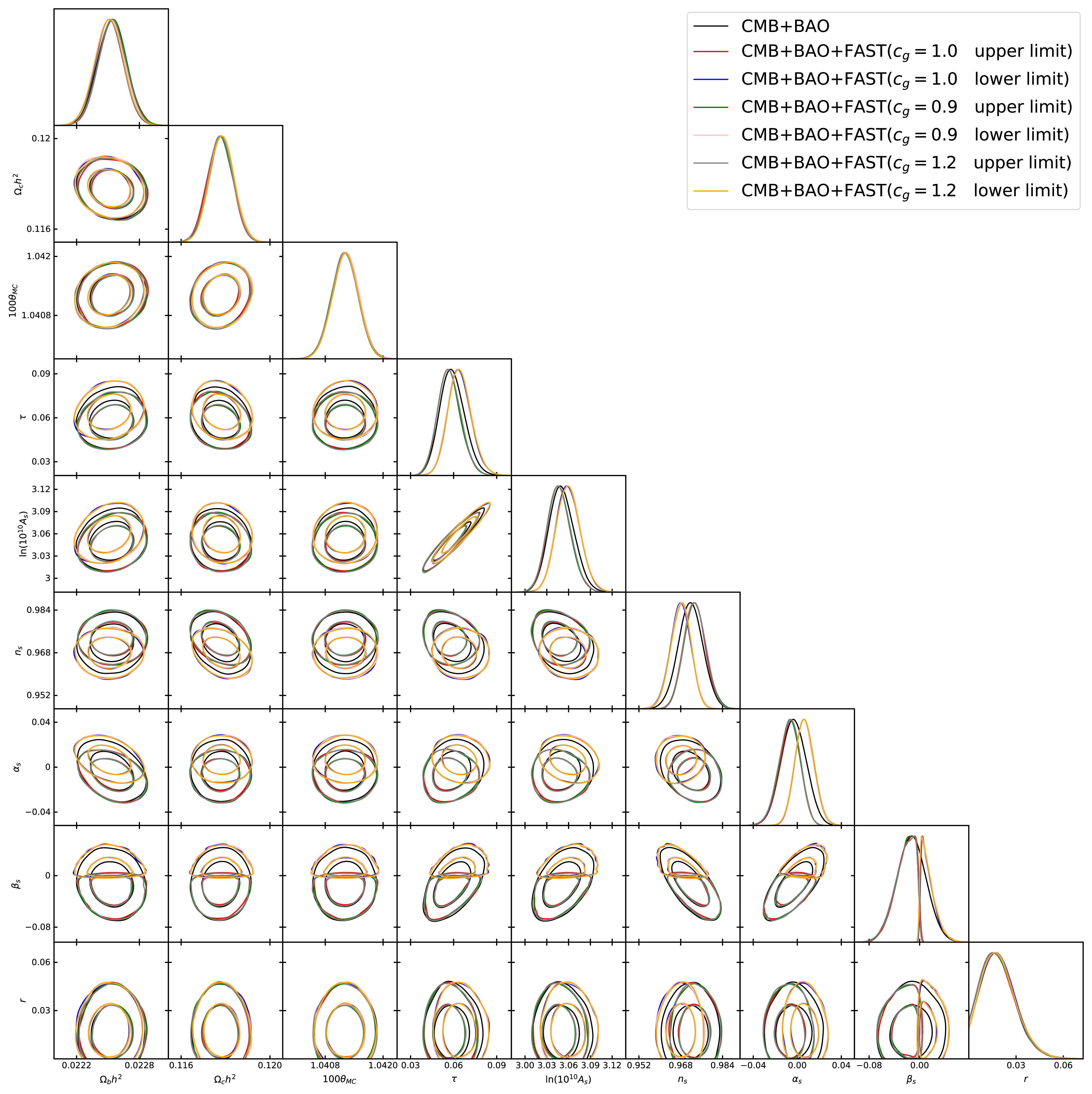
Figure 4. (color online) The contour plots and likelihood distributions for cosmological parameters in the ΛCDM+
$ \alpha_s $ +$ \beta_s $ +r model are shown at the 68% and 95% confidence levels, derived from the following dataset combinations: CMB+BAO; CMB+BAO+FAST ($ c_g=1.0 $ , upper limit); CMB+BAO+FAST ($ c_g=1.0 $ , lower limit); CMB+BAO+FAST ($ c_g=0.9 $ , upper limit); CMB+BAO+FAST ($ c_g=0.9 $ , lower limit); CMB+BAO+FAST ($ c_g=1.2 $ , upper limit); and CMB+BAO+FAST ($ c_g=1.2 $ , lower limit). The solid lines in the likelihood distributions represent the constraints from the CMB+BAO+FAST datasets, while the dashed lines represent the constraints from the CMB+BAO datasets.In the ΛCDM+r model, combining CMB+BAO+ SKA datasets yields a constraint on the scalar spectral index of
$ n_s=0.9598^{+0.0013}_{-0.0009} $ in the upper-limit scenario, in which scalar-induced gravitational waves propagate at the speed of light. This constraint becomes$ n_s =0.9697\pm {0.0033} $ in the lower-limit scenario. Relative to the constraint from CMB+BAO alone, the value of$ n_s $ in the upper-limit scenario exhibits a notable shift, suggesting that$ n_s $ may serve as a diagnostic for the detection of scalar-induced gravitational waves. Detailed values are provided in Table 1. The contour plots and likelihood distributions of cosmological parameters from CMB+BAO+SKA ($ c_g=1.0$ lower limit) remain largely consistent with those derived from CMB+BAO. In contrast, the contour plots and likelihood distributions from CMB+BAO+SKA ($ c_g=1.0$ upper limit) differ noticeably from those of CMB+BAO, as depicted in Fig. 2. Additionally, we consider scalar-induced gravitational waves propagating at speeds different from the speed of light, as shown in Table 2 and Fig. 2. These numerical findings clearly demonstrate the significant influence of the upper and lower limits provided by SKA.In the ΛCDM+
$ \alpha_s $ +r model, the scalar spectral index and the running of the scalar spectral index are constrained to$ n_s=0.9687\pm{0.0034} $ and$ \alpha_s=-0.0071_{-0.0024}^{+0.0060} $ , respectively, from the combination of CMB+BAO+SKA datasets in the upper-limit scenario, in which scalar-induced gravitational waves propagate at the speed of light. The constraints become$ n_s=0.9706^{+0.0034}_{-0.0033} $ and$ \alpha_s= 0.0063^{+0.0032}_{-0.0071} $ in the lower-limit scenario. A comparison with constraints from the CMB+BAO combination reveals notable shifts in$ \alpha_s $ . Detailed values can be found in Table 3. The contour plots and likelihood distributions of$ \alpha_s $ show a preference for positive values in the lower-limit scenario, whereas they favor negative values in the upper-limit scenario, as depicted in Fig. 3. Additionally, we analyze cases in which scalar-induced gravitational waves propagate at speeds different from the speed of light, with results summarized in Table 4 and Fig. 3.In the ΛCDM+
$ \alpha_s $ +$ \beta_s $ +r model, the scalar spectral index, its running, and its running of the running are constrained as follows:$ n_s=0.9733\pm0.0041 $ ,$ \alpha_s= -0.0068_{-0.009}^{+0.010} $ , and$ \beta_s=-0.0232^{+0.021}_{-0.010} $ , derived from the combination of CMB+BAO+FAST datasets in the upper-limit scenario, where scalar-induced gravitational waves propagate at the speed of light. These values shift to$ n_s=0.9679\pm{0.0039} $ ,$ \alpha_s=0.0068\pm{0.009} $ , and$ \beta_s=0.0147^{+0.006}_{-0.015} $ in the lower-limit scenario. A comparison with constraints obtained solely from the CMB+BAO datasets shows significant differences, particularly for$ \alpha_s $ and$ \beta_s $ . Detailed numerical values are summarized in Table 5. The contour plots and likelihood distributions of$ \beta_s $ indicate predominantly positive constraints in the lower-limit scenario, whereas they favor negative values in the upper-limit scenario, as depicted in Fig. 4. Additionally, we consider scalar-induced gravitational waves propagating at speeds different from the speed of light, as shown in Table 6 and Fig. 4. These findings underscore the significant impact of the upper and lower limits provided by FAST. In the ΛCDM+$ \alpha_s $ +r model and the ΛCDM+$ \alpha_s $ +$ \beta_s $ +r model, the running of the scalar spectral index$ \alpha_s $ and the running of the running of the scalar spectral index$ \beta_s $ exhibit notable variations, indicating potential observational insights. -
In the standard ΛCDM model, the six parameters are the baryon density parameter
$ \Omega_b h^2 $ , the cold dark matter density$ \Omega_c h^2 $ , the angular size of the horizon at the last scattering surface$ \theta_{\rm{MC}} $ , the optical depth τ, the scalar amplitude$ A_s $ and the scalar spectral index$ n_s $ . In the literature, the tensor-to-scalar ratio r is utilized to quantify the tensor amplitude$ A_t $ relative to the scalar amplitude$ A_s $ at the pivot scale, namely$ r\equiv\frac{A_t}{A_s}. $
(20) We use the publicly available Cosmomc code [62] to extend the standard ΛCDM model by incorporating parameters such as the tensor-to-scalar ratio r, the running of the scalar spectral index
$ \alpha_s $ , and the running of the running of the scalar spectral index$ \beta_s $ . In the ΛCDM+r model, the priors for the seven cosmological parameters are set following the default CosmoMC configuration, while the remaining parameters are assigned the following uniform priors:$ \alpha_s\in[-0.5,0.5] $ and$ \beta_s\in[-0.5, 0.5] $ . These parameters are constrained using the combinations of CMB+BAO, along with the upper or lower limits of the stochastic gravitational wave background provided by FAST or SKA. The likelihood for the combined CMB+ BAO dataset includes Planck TTTEEE+lowE+lensing, BICEP/Keck 2018 (BK18), 6dF Galaxy Survey, MGS, SDSS DR12, and DESI Data Release 2 (DESI DR2). The upper or lower bounds for the stochastic gravitational-wave background from FAST or SKA are implemented in the subroutine SetFast within the file CosmologyParameterizations.f90 in the source directory. The upper limits on the primordial scalar amplitude$ A_s $ inferred from SKA observations at$ 3.17\times10^{-10} $ Hz are sensitive to the assumed propagation speed of gravitational waves$ c_g $ . In the ΛCDM+r framework, the limits read$ \begin{aligned} c_g&=1.0:\quad A_s<11.5\times10^{-10}\times(4.09\times10^6)^{1-n_s}, \end{aligned} $
(21) $ \begin{aligned} c_g&=0.8:\quad A_s<9.8\times10^{-10}\times(4.09\times10^6)^{1-n_s}, \end{aligned} $
(22) $ \begin{aligned} c_g&=1.5:\quad A_s<18.3\times10^{-10}\times(4.09\times10^6)^{1-n_s}. \end{aligned} $
(23) When the running of the scalar spectral index,
$ \alpha_s $ , is included (ΛCDM+$ \alpha_s $ +r), the corresponding expressions take the following form:$ \begin{aligned} c_g&=1.0:\quad A_s<11.64\times10^{-10}\times(4.09\times10^6)^{1-n_s-7.61\alpha_s}, \end{aligned} $
(24) $ \begin{aligned} c_g&=0.8:\quad A_s<9.84\times10^{-10}\times(4.09\times10^6)^{1-n_s-7.61\alpha_s}, \end{aligned} $
(25) $ \begin{aligned} c_g&=1.5:\quad A_s<18.89\times10^{-10}\times(4.09\times10^6)^{1-n_s-7.61\alpha_s}. \end{aligned} $
(26) Finally, within the extended ΛCDM+
$ \alpha_s $ +$ \beta_s $ +r model, the limits derived from the FAST data at$ 6.34\times10^{-10} $ Hz are:$ \begin{aligned} c_g&=1.0:\quad A_s<23.77\times10^{-10}\times(8.18\times10^6)^{1-n_s-7.96\alpha_s-42.23\beta_s}, \end{aligned} $
(27) $ \begin{aligned} c_g&=0.9:\quad A_s<10.61\times10^{-10}\times(8.18\times10^6)^{1-n_s-7.96\alpha_s-42.23\beta_s}, \end{aligned} $
(28) $ \begin{aligned} c_g&=1.2:\quad A_s<12.66\times10^{-10}\times(8.18\times10^6)^{1-n_s-7.96\alpha_s-42.23\beta_s}. \end{aligned} $
(29) In this analysis, SKA data are used to constrain the ΛCDM+r and ΛCDM+
$ \alpha_s $ +r models; in these parameter spaces, the inclusion of FAST data does not provide tighter constraints than those from the CMB+BAO dataset alone. For the extended ΛCDM+$ \alpha_s $ +$ \beta_s $ +r model, FAST data are used, since the corresponding SKA constraints are much stronger than those obtained from CMB+BAO data. The numerical results are presented in Tables 1 to 6 and Figs. 2 to 4.Parameter CMB+BAO+SKA CMB+BAO+SKA
($c_g=1.0$ upper limit)CMB+BAO+SKA
($c_g=1.0$ lower limit)$ \Omega_bh^2 $ $ 0.02253\pm0.00012 $ $ 0.02247\pm0.00012 $ $ 0.02253\pm0.00012 $ $ \Omega_ch^2 $ $ 0.11783\pm{0.0006} $ $ 0.11850\pm{0.0005} $ $ 0.11782\pm{0.0006} $ $ 100\theta_{{\rm{MC}}} $ $ 1.04122\pm0.00027 $ $ 1.04117\pm0.00027 $ $ 1.04123\pm0.00027 $ τ $ 0.0619^{+0.0068}_{-0.0079} $ $ 0.0527\pm0.0060 $ $ 0.0616^{+0.0069}_{-0.0081} $ $ \ln(10^{10}A_s) $ $ 3.056^{+0.014}_{-0.016} $ $ 3.039^{+0.013}_{-0.012} $ $ 3.055^{+0.014}_{-0.016} $ $ n_s $ $ 0.9698^{+0.0033}_{-0.0032} $ $ 0.9598^{+0.0013}_{-0.0009} $ $ 0.9697\pm{0.0033} $ $ r_{0.05} $ (95% CL)$<0.039 $ $<0.038 $ $<0.040 $ Table 1. The 68% confidence limits on the cosmological parameters of the ΛCDM+r model are derived from the following dataset combinations: CMB+BAO, CMB+BAO+SKA(
$ c_g=1.0$ upper limit), and CMB+BAO+SKA($ c_g=1.0$ lower limit).Parameter CMB+BAO+FAST
($c_g=0.9 $ upper limit)CMB+BAO+FAST
($c_g=0.9$ lower limit)CMB+BAO+FAST
($c_g=1.2$ upper limit)CMB+BAO+FAST
($c_g=1.2$ lower limit)$ \Omega_bh^2 $ $ 0.02254^{+0.00013}_{-0.00014} $ $ 0.02251\pm0.00014 $ $ 0.02254\pm0.00013 $ $ 0.02251\pm0.00013 $ $ \Omega_ch^2 $ $ 0.11777\pm0.0006 $ $ 0.11783\pm{0.0006} $ $ 0.11777\pm0.0006 $ $ 0.11782^{+0.0005}_{-0.0006} $ $ 100\theta_{{\rm{MC}}} $ $ 1.04120\pm0.00027 $ $ 1.04122^{+0.00027}_{-0.00028} $ $ 1.04121\pm0.00027 $ $ 1.04122\pm0.00027 $ τ $ 0.0570_{-0.0088}^{+0.0072} $ $ 0.0642_{-0.0089}^{+0.0078} $ $ 0.0571^{+0.0079}_{-0.0087} $ $ 0.0643^{+0.0075}_{-0.0089} $ $ \ln(10^{10}A_s) $ $ 3.047_{-0.017}^{+0.015} $ $ 3.060_{-0.017}^{+0.016} $ $ 3.047_{-0.017}^{+0.016} $ $ 3.060_{-0.018}^{+0.016} $ $ n_s $ $ 0.9735\pm0.0042 $ $ 0.9680\pm0.0039 $ $ 0.9734\pm0.0042 $ $ 0.9680_{-0.0038}^{+0.0041} $ $ \alpha_s $ $ -0.0073_{-0.009}^{+0.011} $ $ 0.0065_{-0.009}^{+0.008} $ $ -0.0072^{+0.011}_{-0.009} $ $ 0.0065\pm0.009 $ $ \beta_s $ $ -0.0243_{-0.010}^{+0.022} $ $ 0.0144_{-0.015}^{+0.006} $ $ -0.0242^{+0.022}_{-0.010} $ $ 0.0142_{-0.015}^{+0.006} $ $ r_{0.05} $ (95% CL)$<0.038 $ $<0.039 $ $<0.038 $ $<0.039 $ Table 6. The 68% confidence limits on the cosmological parameters for the ΛCDM+
$ \alpha_s $ +$ \beta_s $ +r model are derived from the following dataset combinations: CMB+BAO+FAST ($ c_g=0.9$ upper limit), CMB+BAO+FAST ($ c_g=0.9$ lower limit), CMB+BAO+FAST ($ c_g=1.2$ upper limit), and CMB+BAO+FAST ($ c_g=1.2$ lower limit).
Figure 2. (color online) Contour plots and likelihood distributions of the cosmological parameters in the ΛCDM+r model are shown at the 68% and 95% confidence levels, derived from the following dataset combinations: CMB+BAO; CMB+BAO+SKA(
$ c_g=1.0$ upper limit); CMB+BAO+SKA ($ c_g=1.0$ lower limit); CMB+BAO+SKA ($ c_g=0.8$ upper limit); CMB+BAO+SKA ($ c_g=0.8$ lower limit); CMB+BAO+SKA ($ c_g=1.5$ upper limit); and CMB+BAO+SKA ($ c_g=1.5$ lower limit). Solid lines in the likelihood distributions indicate the constraints from the CMB+BAO+SKA combinations, while dashed lines indicate those from CMB+BAO.
Figure 4. (color online) The contour plots and likelihood distributions for cosmological parameters in the ΛCDM+
$ \alpha_s $ +$ \beta_s $ +r model are shown at the 68% and 95% confidence levels, derived from the following dataset combinations: CMB+BAO; CMB+BAO+FAST ($ c_g=1.0 $ , upper limit); CMB+BAO+FAST ($ c_g=1.0 $ , lower limit); CMB+BAO+FAST ($ c_g=0.9 $ , upper limit); CMB+BAO+FAST ($ c_g=0.9 $ , lower limit); CMB+BAO+FAST ($ c_g=1.2 $ , upper limit); and CMB+BAO+FAST ($ c_g=1.2 $ , lower limit). The solid lines in the likelihood distributions represent the constraints from the CMB+BAO+FAST datasets, while the dashed lines represent the constraints from the CMB+BAO datasets.In the ΛCDM+r model, combining CMB+BAO+ SKA datasets yields a constraint on the scalar spectral index of
$ n_s=0.9598^{+0.0013}_{-0.0009} $ in the upper-limit scenario, in which scalar-induced gravitational waves propagate at the speed of light. This constraint becomes$ n_s =0.9697\pm {0.0033} $ in the lower-limit scenario. Relative to the constraint from CMB+BAO alone, the value of$ n_s $ in the upper-limit scenario exhibits a notable shift, suggesting that$ n_s $ may serve as a diagnostic for the detection of scalar-induced gravitational waves. Detailed values are provided in Table 1. The contour plots and likelihood distributions of cosmological parameters from CMB+BAO+SKA ($ c_g=1.0$ lower limit) remain largely consistent with those derived from CMB+BAO. In contrast, the contour plots and likelihood distributions from CMB+BAO+SKA ($ c_g=1.0$ upper limit) differ noticeably from those of CMB+BAO, as depicted in Fig. 2. Additionally, we consider scalar-induced gravitational waves propagating at speeds different from the speed of light, as shown in Table 2 and Fig. 2. These numerical findings clearly demonstrate the significant influence of the upper and lower limits provided by SKA.Parameter CMB+BAO+SKA
($c_g=0.8 $ upper limit)CMB+BAO+SKA
($c_g=0.8$ lower limit)CMB+BAO+SKA
($c_g=1.5$ upper limit)CMB+BAO+SKA
($c_g=1.5$ lower limit)$ \Omega_bh^2 $ $ 0.02242\pm0.00012 $ $ 0.02253\pm0.00012 $ $ 0.02253\pm0.00012 $ $ 0.02265\pm0.00013 $ $ \Omega_ch^2 $ $ 0.11912\pm0.0005 $ $ 0.11782\pm{0.0006} $ $ 0.11782\pm{0.0006} $ $ 0.11644\pm{0.0005} $ $ 100\theta_{{\rm{MC}}} $ $ 1.04112\pm0.00028 $ $ 1.04122\pm0.00028 $ $ 1.04123\pm0.00027 $ $ 1.04131\pm0.00027 $ τ $ 0.0451^{+0.0070}_{-0.0061} $ $ 0.0621^{+0.0070}_{-0.0080} $ $ 0.0618^{+0.0069}_{-0.0079} $ $ 0.0857^{+0.0076}_{-0.0077} $ $ \ln(10^{10}A_s) $ $ 3.026\pm0.013 $ $ 3.056^{+0.014}_{-0.016} $ $ 3.056^{+0.014}_{-0.016} $ $ 3.099\pm0.015 $ $ n_s $ $ 0.9506\pm{0.0010} $ $ 0.9697\pm{0.0033} $ $ 0.9698\pm0.0033 $ $ 0.9880\pm0.0011 $ $ r_{0.05} $ (95% CL)$<0.036 $ $<0.039 $ $<0.039 $ $<0.040 $ Table 2. The 68% confidence limits on the cosmological parameters of the ΛCDM+r model are obtained from the following dataset combinations: CMB+BAO+SKA (
$ c_g=0.8$ upper limit), CMB+BAO+SKA ($ c_g=0.8$ lower limit), CMB+BAO+SKA ($ c_g=1.5$ upper limit), and CMB+BAO+SKA ($ c_g=1.5$ lower limit).In the ΛCDM+
$ \alpha_s $ +r model, the scalar spectral index and the running of the scalar spectral index are constrained to$ n_s=0.9687\pm{0.0034} $ and$ \alpha_s=-0.0071_{-0.0024}^{+0.0060} $ , respectively, from the combination of CMB+BAO+SKA datasets in the upper-limit scenario, in which scalar-induced gravitational waves propagate at the speed of light. The constraints become$ n_s=0.9706^{+0.0034}_{-0.0033} $ and$ \alpha_s= 0.0063^{+0.0032}_{-0.0071} $ in the lower-limit scenario. A comparison with constraints from the CMB+BAO combination reveals notable shifts in$ \alpha_s $ . Detailed values can be found in Table 3. The contour plots and likelihood distributions of$ \alpha_s $ show a preference for positive values in the lower-limit scenario, whereas they favor negative values in the upper-limit scenario, as depicted in Fig. 3. Additionally, we analyze cases in which scalar-induced gravitational waves propagate at speeds different from the speed of light, with results summarized in Table 4 and Fig. 3.Parameter CMB+BAO CMB+BAO+SKA
($c_g=1.0$ upper limit)CMB+BAO+SKA
($c_g=1.0$ lower limit)$ \Omega_bh^2 $ $ 0.02253\pm0.00014 $ $ 0.02258\pm0.00013 $ $ 0.02249\pm0.00013 $ $ \Omega_ch^2 $ $ 0.11782\pm0.0006 $ $ 0.11784\pm0.0006 $ $ 0.11778\pm0.0006 $ $ 100\theta_{{\rm{MC}}} $ $ 1.04123\pm0.00027 $ $ 1.04123\pm0.00027 $ $ 1.04121^{+0.00027}_{-0.00028} $ τ $ 0.0616^{+0.0071}_{-0.0083} $ $ 0.0635^{+0.0073}_{-0.0084} $ $ 0.0605^{+0.0071}_{-0.0081} $ $ \ln(10^{10}A_s) $ $ 3.055_{-0.017}^{+0.015} $ $ 3.060_{-0.016}^{+0.015} $ $ 3.052\pm0.015 $ $ n_s $ $ 0.9700\pm{0.0034} $ $ 0.9687\pm{0.0034} $ $ 0.9706^{+0.0034}_{-0.0033} $ $ \alpha_s $ $ 0.0013\pm0.0080 $ $ -0.0071_{-0.0024}^{+0.0060} $ $ 0.0063^{+0.0032}_{-0.0071} $ $ r_{0.05} $ (95% CL)$<0.039 $ $<0.039 $ $<0.039 $ Table 3. The 68% confidence limits for the cosmological parameters of the ΛCDM+
$ \alpha_s $ +r model are obtained from the combinations CMB+BAO, CMB+BAO+SKA ($ c_g=1.0$ , upper limit), and CMB+BAO+SKA ($ c_g=1.0$ , lower limit) datasets.Parameter CMB+BAO+SKA
($c_g=0.8 $ upper limit)CMB+BAO+SKA
($c_g=0.8$ lower limit)CMB+BAO+SKA
($c_g=1.5$ upper limit)CMB+BAO+SKA
($c_g=1.5$ lower limit)$ \Omega_bh^2 $ $ 0.02259\pm0.00013 $ $ 0.02250\pm0.00013 $ $ 0.02256\pm0.00013 $ $ 0.02248\pm0.00013 $ $ \Omega_ch^2 $ $ 0.11784\pm0.0006 $ $ 0.11778\pm0.0006 $ $ 0.11784\pm0.0006 $ $ 0.11777\pm0.0006 $ $ 100\theta_{{\rm{MC}}} $ $ 1.04122\pm0.00027 $ $ 1.04123^{+0.00027}_{-0.00028} $ $ 1.04122\pm0.00027 $ $ 1.04121\pm0.00027 $ τ $ 0.0634^{+0.0073}_{-0.0081} $ $ 0.0606^{+0.0070}_{-0.0080} $ $ 0.0626^{+0.0070}_{-0.0082} $ $ 0.0602^{+0.0071}_{-0.0077} $ $ \ln(10^{10}A_s) $ $ 3.061\pm0.015 $ $ 3.052\pm0.015 $ $ 3.058^{+0.014}_{-0.017} $ $ 3.051\pm0.015 $ $ n_s $ $ 0.9687\pm0.0033 $ $ 0.9707\pm0.0034 $ $ 0.9691\pm0.0033 $ $ 0.9711\pm0.0033 $ $ \alpha_s $ $ -0.0078_{-0.0021}^{+0.0053} $ $ 0.0058_{-0.0078}^{+0.0036} $ $ -0.0041^{+0.0069}_{-0.0030} $ $ 0.0088_{-0.0059}^{+0.0024} $ $ r_{0.05} $ (95% CL)$<0.039 $ $<0.037 $ $<0.039 $ $<0.039 $ Table 4. The 68% confidence limits on the cosmological parameters for the ΛCDM+
$ \alpha_s $ +r model are obtained from combinations of the CMB+BAO+SKA datasets with$ c_g=0.8$ upper limit,$ c_g=0.8$ lower limit,$ c_g=1.5$ upper limit, and$ c_g=1.5$ lower limit.
Figure 3. (color online) The contour plots and likelihood distributions of cosmological parameters in the ΛCDM+
$ \alpha_s $ +r model are shown at the 68% and 95% confidence levels, derived from the combinations CMB+BAO, CMB+BAO+SKA ($ c_g=1.0$ upper limit), CMB+BAO+SKA ($ c_g=1.0$ lower limit), CMB+BAO+SKA ($ c_g=0.8$ upper limit), CMB+BAO+SKA ($ c_g=0.8$ lower limit), CMB+BAO+SKA ($ c_g=1.5$ upper limit), and CMB+BAO+SKA ($ c_g=1.5$ lower limit). The solid lines in the likelihood distributions represent the constraints from the CMB+BAO+SKA datasets. The dashed lines in the likelihood distributions represent the constraints from the CMB+BAO dataset.In the ΛCDM+
$ \alpha_s $ +$ \beta_s $ +r model, the scalar spectral index, its running, and its running of the running are constrained as follows:$ n_s=0.9733\pm0.0041 $ ,$ \alpha_s= -0.0068_{-0.009}^{+0.010} $ , and$ \beta_s=-0.0232^{+0.021}_{-0.010} $ , derived from the combination of CMB+BAO+FAST datasets in the upper-limit scenario, where scalar-induced gravitational waves propagate at the speed of light. These values shift to$ n_s=0.9679\pm{0.0039} $ ,$ \alpha_s=0.0068\pm{0.009} $ , and$ \beta_s=0.0147^{+0.006}_{-0.015} $ in the lower-limit scenario. A comparison with constraints obtained solely from the CMB+BAO datasets shows significant differences, particularly for$ \alpha_s $ and$ \beta_s $ . Detailed numerical values are summarized in Table 5. The contour plots and likelihood distributions of$ \beta_s $ indicate predominantly positive constraints in the lower-limit scenario, whereas they favor negative values in the upper-limit scenario, as depicted in Fig. 4. Additionally, we consider scalar-induced gravitational waves propagating at speeds different from the speed of light, as shown in Table 6 and Fig. 4. These findings underscore the significant impact of the upper and lower limits provided by FAST. In the ΛCDM+$ \alpha_s $ +r model and the ΛCDM+$ \alpha_s $ +$ \beta_s $ +r model, the running of the scalar spectral index$ \alpha_s $ and the running of the running of the scalar spectral index$ \beta_s $ exhibit notable variations, indicating potential observational insights.Parameter CMB+BAO CMB+BAO+FAST ( $c_g=1.0$ upper limit)CMB+BAO+FAST ( $c_g=1.0$ lower limit)$ \Omega_bh^2 $ $ 0.02254^{+0.00013}_{-0.00014} $ $ 0.02255\pm0.00013 $ $ 0.02251\pm0.00013 $ $ \Omega_ch^2 $ $ 0.11779\pm{0.0006} $ $ 0.11775\pm{0.0006} $ $ 0.11783\pm0.0006 $ $ 100\theta_{{\rm{MC}}} $ $ 1.04121\pm0.00027 $ $ 1.04122\pm0.00027 $ $ 1.04122^{+0.00028}_{-0.00027} $ τ $ 0.0591^{+0.0081}_{-0.0095} $ $ 0.0571^{+0.0072}_{-0.0088} $ $ 0.0642^{+0.0076}_{-0.0087} $ $ \ln(10^{10}A_s) $ $ 3.051^{+0.016}_{-0.019} $ $ 3.047^{+0.015}_{-0.018} $ $ 3.059^{+0.016}_{-0.018} $ $ n_s $ $ 0.9718\pm{0.0047} $ $ 0.9733\pm0.0041 $ $ 0.9679\pm{0.0039} $ $ \alpha_s $ $ -0.0033^{+0.012}_{-0.011} $ $ -0.0068_{-0.009}^{+0.010} $ $ 0.0068\pm{0.009} $ $ \beta_s $ $ -0.0131\pm0.023 $ $ -0.0232^{+0.021}_{-0.010} $ $ 0.0147^{+0.006}_{-0.015} $ $ r_{0.05} $ (95% CL)$<0.039 $ $<0.038 $ $<0.039 $ Table 5. The 68% confidence limits on the cosmological parameters for the ΛCDM+
$ \alpha_s $ +$ \beta_s $ +r model are obtained from combinations of the CMB+BAO, CMB+BAO+FAST ($ c_g=1.0$ upper limit), and CMB+BAO+FAST ($ c_g=1.0$ lower limit) datasets. -
In the standard ΛCDM model, the six parameters are the baryon density parameter
$ \Omega_b h^2 $ , the cold dark matter density$ \Omega_c h^2 $ , the angular size of the horizon at the last scattering surface$ \theta_{\rm{MC}} $ , the optical depth τ, the scalar amplitude$ A_s $ and the scalar spectral index$ n_s $ . In the literature, the tensor-to-scalar ratio r is utilized to quantify the tensor amplitude$ A_t $ relative to the scalar amplitude$ A_s $ at the pivot scale, namely$ r\equiv\frac{A_t}{A_s}. $
(20) We use the publicly available Cosmomc code [62] to extend the standard ΛCDM model by incorporating parameters such as the tensor-to-scalar ratio r, the running of the scalar spectral index
$ \alpha_s $ , and the running of the running of the scalar spectral index$ \beta_s $ . In the ΛCDM+r model, the priors for the seven cosmological parameters are set following the default CosmoMC configuration, while the remaining parameters are assigned the following uniform priors:$ \alpha_s\in[-0.5,0.5] $ and$ \beta_s\in[-0.5, 0.5] $ . These parameters are constrained using the combinations of CMB+BAO, along with the upper or lower limits of the stochastic gravitational wave background provided by FAST or SKA. The likelihood for the combined CMB+BAO dataset includes Planck TTTEEE+lowE+lensing, BICEP/Keck 2018 (BK18), 6dF Galaxy Survey, MGS, SDSS DR12, and DESI Data Release 2 (DESI DR2). The upper or lower bounds for the stochastic gravitational-wave background from FAST or SKA are implemented in the subroutine SetFast within the file CosmologyParameterizations.f90 in the source directory. The upper limits on the primordial scalar amplitude$ A_s $ inferred from SKA observations at$ 3.17\times10^{-10} $ Hz are sensitive to the assumed propagation speed of gravitational waves$ c_g $ . In the ΛCDM+r framework, the limits read$ \begin{aligned} c_g&=1.0:\quad A_s<11.5\times10^{-10}\times(4.09\times10^6)^{1-n_s}, \end{aligned} $
(21) $ \begin{aligned} c_g&=0.8:\quad A_s<9.8\times10^{-10}\times(4.09\times10^6)^{1-n_s}, \end{aligned} $
(22) $ \begin{aligned} c_g&=1.5:\quad A_s<18.3\times10^{-10}\times(4.09\times10^6)^{1-n_s}. \end{aligned} $
(23) When the running of the scalar spectral index,
$ \alpha_s $ , is included (ΛCDM+$ \alpha_s $ +r), the corresponding expressions take the following form:$ \begin{aligned} c_g&=1.0:\quad A_s<11.64\times10^{-10}\times(4.09\times10^6)^{1-n_s-7.61\alpha_s}, \end{aligned} $
(24) $ \begin{aligned} c_g&=0.8:\quad A_s<9.84\times10^{-10}\times(4.09\times10^6)^{1-n_s-7.61\alpha_s}, \end{aligned} $
(25) $ \begin{aligned} c_g&=1.5:\quad A_s<18.89\times10^{-10}\times(4.09\times10^6)^{1-n_s-7.61\alpha_s}. \end{aligned} $
(26) Finally, within the extended ΛCDM+
$ \alpha_s $ +$ \beta_s $ +r model, the limits derived from the FAST data at$ 6.34\times10^{-10} $ Hz are:$ \begin{aligned} c_g&=1.0:\quad A_s<23.77\times10^{-10}\times(8.18\times10^6)^{1-n_s-7.96\alpha_s-42.23\beta_s}, \end{aligned} $
(27) $ \begin{aligned} c_g&=0.9:\quad A_s<10.61\times10^{-10}\times(8.18\times10^6)^{1-n_s-7.96\alpha_s-42.23\beta_s}, \end{aligned} $
(28) $ \begin{aligned} c_g&=1.2:\quad A_s<12.66\times10^{-10}\times(8.18\times10^6)^{1-n_s-7.96\alpha_s-42.23\beta_s}. \end{aligned} $
(29) In this analysis, SKA data are used to constrain the ΛCDM+r and ΛCDM+
$ \alpha_s $ +r models; in these parameter spaces, the inclusion of FAST data does not provide tighter constraints than those from the CMB+BAO dataset alone. For the extended ΛCDM+$ \alpha_s $ +$ \beta_s $ +r model, FAST data are used, since the corresponding SKA constraints are much stronger than those obtained from CMB+BAO data. The numerical results are presented in Tables 1 to 6 and Figures 2 to 4.Parameter CMB+BAO CMB+BAO+SKA
($c_g=1.0$ upper limit)CMB+BAO+SKA
($c_g=1.0$ lower limit)$ \Omega_bh^2 $ $ 0.02253\pm0.00012 $ $ 0.02247\pm0.00012 $ $ 0.02253\pm0.00012 $ $ \Omega_ch^2 $ $ 0.11783\pm{0.0006} $ $ 0.11850\pm{0.0005} $ $ 0.11782\pm{0.0006} $ $ 100\theta_{{\rm{MC}}} $ $ 1.04122\pm0.00027 $ $ 1.04117\pm0.00027 $ $ 1.04123\pm0.00027 $ τ $ 0.0619^{+0.0068}_{-0.0079} $ $ 0.0527\pm0.0060 $ $ 0.0616^{+0.0069}_{-0.0081} $ $ \ln(10^{10}A_s) $ $ 3.056^{+0.014}_{-0.016} $ $ 3.039^{+0.013}_{-0.012} $ $ 3.055^{+0.014}_{-0.016} $ $ n_s $ $ 0.9698^{+0.0033}_{-0.0032} $ $ 0.9598^{+0.0013}_{-0.0009} $ $ 0.9697\pm{0.0033} $ $ r_{0.05} $ (95% CL)$<0.039 $ $<0.038 $ $<0.040 $ Table 1. The 68% confidence limits on the cosmological parameters of the ΛCDM+r model are derived from the following dataset combinations: CMB+BAO, CMB+BAO+SKA(
$ c_g=1.0$ upper limit), and CMB+BAO+SKA($ c_g=1.0$ lower limit).Parameter CMB+BAO CMB+BAO+SKA ( $c_g=1.0$ upper limit)CMB+BAO+SKA ( $c_g=1.0$ lower limit)CMB+BAO+SKA ( $c_g=0.8$ upper limit)$ \Omega_bh^2 $ $ 0.02254^{+0.00013}_{-0.00014} $ $ 0.02251\pm0.00014 $ $ 0.02254\pm0.00013 $ $ 0.02251\pm0.00013 $ $ \Omega_ch^2 $ $ 0.11777\pm0.0006 $ $ 0.11783\pm{0.0006} $ $ 0.11777\pm0.0006 $ $ 0.11782^{+0.0005}_{-0.0006} $ $ 100\theta_{{\rm{MC}}} $ $ 1.04120\pm0.00027 $ $ 1.04122^{+0.00027}_{-0.00028} $ $ 1.04121\pm0.00027 $ $ 1.04122\pm0.00027 $ τ $ 0.0570_{-0.0088}^{+0.0072} $ $ 0.0642_{-0.0089}^{+0.0078} $ $ 0.0571^{+0.0079}_{-0.0087} $ $ 0.0643^{+0.0075}_{-0.0089} $ $ \ln(10^{10}A_s) $ $ 3.047_{-0.017}^{+0.015} $ $ 3.060_{-0.017}^{+0.016} $ $ 3.047_{-0.017}^{+0.016} $ $ 3.060_{-0.018}^{+0.016} $ $ n_s $ $ 0.9735\pm0.0042 $ $ 0.9680\pm0.0039 $ $ 0.9734\pm0.0042 $ $ 0.9680_{-0.0038}^{+0.0041} $ $ \alpha_s $ $ -0.0073_{-0.009}^{+0.011} $ $ 0.0065_{-0.009}^{+0.008} $ $ -0.0072^{+0.011}_{-0.009} $ $ 0.0065\pm0.009 $ $ \beta_s $ $ -0.0243_{-0.010}^{+0.022} $ $ 0.0144_{-0.015}^{+0.006} $ $ -0.0242^{+0.022}_{-0.010} $ $ 0.0142_{-0.015}^{+0.006} $ $ r_{0.05} $ (95% CL)$<0.038 $ $<0.039 $ $<0.038 $ $<0.039 $ Table 6. The 68% confidence limits on the cosmological parameters for the ΛCDM+
$ \alpha_s $ +$ \beta_s $ +r model are derived from the following dataset combinations: CMB+BAO+FAST($ c_g=0.9$ upper limit), CMB+BAO+FAST($ c_g=0.9$ lower limit), CMB+BAO+FAST($ c_g=1.2$ upper limit), and CMB+BAO+FAST($ c_g=1.2$ lower limit).
Figure 2. Contour plots and likelihood distributions of the cosmological parameters in the ΛCDM+r model are shown at the 68% and 95% confidence levels, derived from the following dataset combinations: CMB+BAO; CMB+BAO+SKA(
$ c_g=1.0$ upper limit); CMB+BAO+SKA($ c_g=1.0$ lower limit); CMB+BAO+SKA($ c_g=0.8$ upper limit); CMB+BAO+SKA($ c_g=0.8$ lower limit); CMB+BAO+SKA($ c_g=1.5$ upper limit); and CMB+BAO+SKA($ c_g=1.5$ lower limit). Solid lines in the likelihood distributions indicate the constraints from the CMB+BAO+SKA combinations, while dashed lines indicate those from CMB+BAO.
Figure 4. The contour plots and likelihood distributions for cosmological parameters in the ΛCDM+
$ \alpha_s $ +$ \beta_s $ +r model are shown at the 68% and 95% confidence levels, derived from the following dataset combinations: CMB+BAO; CMB+BAO+FAST ($ c_g=1.0 $ , upper limit); CMB+BAO+FAST ($ c_g=1.0 $ , lower limit); CMB+BAO+FAST ($ c_g=0.9 $ , upper limit); CMB+BAO+FAST ($ c_g=0.9 $ , lower limit); CMB+BAO+FAST ($ c_g=1.2 $ , upper limit); and CMB+BAO+FAST ($ c_g=1.2 $ , lower limit). The solid lines in the likelihood distributions represent the constraints from the CMB+BAO+FAST datasets, while the dashed lines represent the constraints from the CMB+BAO datasets.In the ΛCDM+r model, combining CMB+BAO+SKA datasets yields a constraint on the scalar spectral index of
$ n_s=0.9598^{+0.0013}_{-0.0009} $ in the upper-limit scenario, in which scalar-induced gravitational waves propagate at the speed of light. This constraint becomes$ n_s =0.9697\pm{0.0033} $ in the lower-limit scenario. Relative to the constraint from CMB+BAO alone, the value of$ n_s $ in the upper-limit scenario exhibits a notable shift, suggesting that$ n_s $ may serve as a diagnostic for the detection of scalar-induced gravitational waves. Detailed values are provided in Table 1. The contour plots and likelihood distributions of cosmological parameters from CMB+BAO+SKA($ c_g=1.0$ lower limit) remain largely consistent with those derived from CMB+BAO. In contrast, the contour plots and likelihood distributions from CMB+BAO+SKA($ c_g=1.0$ upper limit) differ noticeably from those of CMB+BAO, as depicted in Figure 2. Additionally, we consider scalar-induced gravitational waves propagating at speeds different from the speed of light, as shown in Table 2 and Figure 2. These numerical findings clearly demonstrate the significant influence of the upper and lower limits provided by SKA.Parameter CMB+BAO CMB+BAO+SKA
($c_g=1.0$ upper limit)CMB+BAO+SKA
($c_g=1.0$ lower limit)CMB+BAO+SKA
($c_g=0.8$ upper limit)$ \Omega_bh^2 $ $ 0.02242\pm0.00012 $ $ 0.02253\pm0.00012 $ $ 0.02253\pm0.00012 $ $ 0.02265\pm0.00013 $ $ \Omega_ch^2 $ $ 0.11912\pm0.0005 $ $ 0.11782\pm{0.0006} $ $ 0.11782\pm{0.0006} $ $ 0.11644\pm{0.0005} $ $ 100\theta_{{\rm{MC}}} $ $ 1.04112\pm0.00028 $ $ 1.04122\pm0.00028 $ $ 1.04123\pm0.00027 $ $ 1.04131\pm0.00027 $ τ $ 0.0451^{+0.0070}_{-0.0061} $ $ 0.0621^{+0.0070}_{-0.0080} $ $ 0.0618^{+0.0069}_{-0.0079} $ $ 0.0857^{+0.0076}_{-0.0077} $ $ \ln(10^{10}A_s) $ $ 3.026\pm0.013 $ $ 3.056^{+0.014}_{-0.016} $ $ 3.056^{+0.014}_{-0.016} $ $ 3.099\pm0.015 $ $ n_s $ $ 0.9506\pm{0.0010} $ $ 0.9697\pm{0.0033} $ $ 0.9698\pm0.0033 $ $ 0.9880\pm0.0011 $ $ r_{0.05} $ (95% CL)$<0.036 $ $<0.039 $ $<0.039 $ $<0.040 $ Table 2. The 68% confidence limits on the cosmological parameters of the ΛCDM+r model are obtained from the following dataset combinations: CMB+BAO+SKA (
$ c_g=0.8$ upper limit), CMB+BAO+SKA ($ c_g=0.8$ lower limit), CMB+BAO+SKA ($ c_g=1.5$ upper limit), and CMB+BAO+SKA ($ c_g=1.5$ lower limit).In the ΛCDM+
$ \alpha_s $ +r model, the scalar spectral index and the running of the scalar spectral index are constrained to$ n_s=0.9687\pm{0.0034} $ and$ \alpha_s=-0.0071_{-0.0024}^{+0.0060} $ , respectively, from the combination of CMB+BAO+SKA datasets in the upper-limit scenario, in which scalar-induced gravitational waves propagate at the speed of light. The constraints become$ n_s=0.9706^{+0.0034}_{-0.0033} $ and$ \alpha_s=0.0063^{+0.0032}_{-0.0071} $ in the lower-limit scenario. A comparison with constraints from the CMB+BAO combination reveals notable shifts in$ \alpha_s $ . Detailed values can be found in Table 3. The contour plots and likelihood distributions of$ \alpha_s $ show a preference for positive values in the lower-limit scenario, whereas they favor negative values in the upper-limit scenario, as depicted in Figure 3. Additionally, we analyze cases in which scalar-induced gravitational waves propagate at speeds different from the speed of light, with results summarized in Table 4 and Figure 3.Parameter CMB+BAO CMB+BAO+SKA
($c_g=1.0$ upper limit)CMB+BAO+SKA
($c_g=1.0$ lower limit)$ \Omega_bh^2 $ $ 0.02253\pm0.00014 $ $ 0.02258\pm0.00013 $ $ 0.02249\pm0.00013 $ $ \Omega_ch^2 $ $ 0.11782\pm0.0006 $ $ 0.11784\pm0.0006 $ $ 0.11778\pm0.0006 $ $ 100\theta_{{\rm{MC}}} $ $ 1.04123\pm0.00027 $ $ 1.04123\pm0.00027 $ $ 1.04121^{+0.00027}_{-0.00028} $ τ $ 0.0616^{+0.0071}_{-0.0083} $ $ 0.0635^{+0.0073}_{-0.0084} $ $ 0.0605^{+0.0071}_{-0.0081} $ $ \ln(10^{10}A_s) $ $ 3.055_{-0.017}^{+0.015} $ $ 3.060_{-0.016}^{+0.015} $ $ 3.052\pm0.015 $ $ n_s $ $ 0.9700\pm{0.0034} $ $ 0.9687\pm{0.0034} $ $ 0.9706^{+0.0034}_{-0.0033} $ $ \alpha_s $ $ 0.0013\pm0.0080 $ $ -0.0071_{-0.0024}^{+0.0060} $ $ 0.0063^{+0.0032}_{-0.0071} $ $ r_{0.05} $ (95% CL)$<0.039 $ $<0.039 $ $<0.039 $ Table 3. The 68% confidence limits for the cosmological parameters of the ΛCDM+
$ \alpha_s $ +r model are obtained from the combinations CMB+BAO, CMB+BAO+SKA ($ c_g=1.0$ , upper limit), and CMB+BAO+SKA ($ c_g=1.0$ , lower limit) datasets.Parameter CMB+BAO CMB+BAO+SKA ( $c_g=1.0$ upper limit)CMB+BAO+SKA ( $c_g=1.0$ lower limit)CMB+BAO+SKA ( $c_g=0.8$ upper limit)$ \Omega_bh^2 $ $ 0.02259\pm0.00013 $ $ 0.02250\pm0.00013 $ $ 0.02256\pm0.00013 $ $ 0.02248\pm0.00013 $ $ \Omega_ch^2 $ $ 0.11784\pm0.0006 $ $ 0.11778\pm0.0006 $ $ 0.11784\pm0.0006 $ $ 0.11777\pm0.0006 $ $ 100\theta_{{\rm{MC}}} $ $ 1.04122\pm0.00027 $ $ 1.04123^{+0.00027}_{-0.00028} $ $ 1.04122\pm0.00027 $ $ 1.04121\pm0.00027 $ τ $ 0.0634^{+0.0073}_{-0.0081} $ $ 0.0606^{+0.0070}_{-0.0080} $ $ 0.0626^{+0.0070}_{-0.0082} $ $ 0.0602^{+0.0071}_{-0.0077} $ $ \ln(10^{10}A_s) $ $ 3.061\pm0.015 $ $ 3.052\pm0.015 $ $ 3.058^{+0.014}_{-0.017} $ $ 3.051\pm0.015 $ $ n_s $ $ 0.9687\pm0.0033 $ $ 0.9707\pm0.0034 $ $ 0.9691\pm0.0033 $ $ 0.9711\pm0.0033 $ $ \alpha_s $ $ -0.0078_{-0.0021}^{+0.0053} $ $ 0.0058_{-0.0078}^{+0.0036} $ $ -0.0041^{+0.0069}_{-0.0030} $ $ 0.0088_{-0.0059}^{+0.0024} $ $ r_{0.05} $ (95% CL)$<0.039 $ $<0.037 $ $<0.039 $ $<0.039 $ Table 4. The 68% confidence limits on the cosmological parameters for the ΛCDM+
$ \alpha_s $ +r model are obtained from combinations of the CMB+BAO+SKA datasets with$ c_g=0.8$ upper limit,$ c_g=0.8$ lower limit,$ c_g=1.5$ upper limit, and$ c_g=1.5$ lower limit.In the ΛCDM+
$ \alpha_s $ +$ \beta_s $ +r model, the scalar spectral index, its running, and its running of the running are constrained as follows:$ n_s=0.9733\pm0.0041 $ ,$ \alpha_s=-0.0068_{-0.009}^{+0.010} $ , and$ \beta_s=-0.0232^{+0.021}_{-0.010} $ , derived from the combination of CMB+BAO+FAST datasets in the upper-limit scenario, where scalar-induced gravitational waves propagate at the speed of light. These values shift to$ n_s=0.9679\pm{0.0039} $ ,$ \alpha_s=0.0068\pm{0.009} $ , and$ \beta_s=0.0147^{+0.006}_{-0.015} $ in the lower-limit scenario. A comparison with constraints obtained solely from the CMB+BAO datasets shows significant differences, particularly for$ \alpha_s $ and$ \beta_s $ . Detailed numerical values are summarized in Table 5. The contour plots and likelihood distributions of$ \beta_s $ indicate predominantly positive constraints in the lower-limit scenario, whereas they favor negative values in the upper-limit scenario, as depicted in Figure 4. Additionally, we consider scalar-induced gravitational waves propagating at speeds different from the speed of light, as shown in Table 6 and Figure 4. These findings underscore the significant impact of the upper and lower limits provided by FAST. In the ΛCDM+$ \alpha_s $ +r model and the ΛCDM+$ \alpha_s $ +$ \beta_s $ +r model, the running of the scalar spectral index$ \alpha_s $ and the running of the running of the scalar spectral index$ \beta_s $ exhibit notable variations, indicating potential observational insights.Parameter CMB+BAO CMB+BAO+SKA ( $c_g=1.0$ upper limit)CMB+BAO+SKA ( $c_g=1.0$ lower limit)$ \Omega_bh^2 $ $ 0.02254^{+0.00013}_{-0.00014} $ $ 0.02255\pm0.00013 $ $ 0.02251\pm0.00013 $ $ \Omega_ch^2 $ $ 0.11779\pm{0.0006} $ $ 0.11775\pm{0.0006} $ $ 0.11783\pm0.0006 $ $ 100\theta_{{\rm{MC}}} $ $ 1.04121\pm0.00027 $ $ 1.04122\pm0.00027 $ $ 1.04122^{+0.00028}_{-0.00027} $ τ $ 0.0591^{+0.0081}_{-0.0095} $ $ 0.0571^{+0.0072}_{-0.0088} $ $ 0.0642^{+0.0076}_{-0.0087} $ $ \ln(10^{10}A_s) $ $ 3.051^{+0.016}_{-0.019} $ $ 3.047^{+0.015}_{-0.018} $ $ 3.059^{+0.016}_{-0.018} $ $ n_s $ $ 0.9718\pm{0.0047} $ $ 0.9733\pm0.0041 $ $ 0.9679\pm{0.0039} $ $ \alpha_s $ $ -0.0033^{+0.012}_{-0.011} $ $ -0.0068_{-0.009}^{+0.010} $ $ 0.0068\pm{0.009} $ $ \beta_s $ $ -0.0131\pm0.023 $ $ -0.0232^{+0.021}_{-0.010} $ $ 0.0147^{+0.006}_{-0.015} $ $ r_{0.05} $ (95% CL)$<0.039 $ $<0.038 $ $<0.039 $ Table 5. The 68% confidence limits on the cosmological parameters for the ΛCDM+
$ \alpha_s $ +$ \beta_s $ +r model are obtained from combinations of the CMB+BAO, CMB+BAO+FAST($ c_g=1.0$ upper limit), and CMB+BAO+FAST($ c_g=1.0$ lower limit) datasets. -
Scalar-induced gravitational waves from the early universe are a key prediction of various inflationary models, in which quantum fluctuations during inflation generate a stochastic gravitational-wave background. These waves imprint specific signatures in the polarization of the CMB and in the large-scale structure of the universe. Such signatures offer complementary observational avenues to confirm their existence and investigate their properties. Detecting scalar-induced gravitational waves requires highly sensitive instruments capable of measuring minute distortions of spacetime.
In this paper, we combine CMB+BAO datasets with upper or lower limits on the stochastic gravitational-wave background provided by FAST or SKA to constrain scalar-induced gravitational waves. In the ΛCDM+r model, the scalar spectral index of the power-law power spectrum is constrained to
$ n_s=0.9598^{+0.0013}_{-0.0009} $ in the upper-limit scenario, derived from the combined CMB+BAO+SKA datasets and assuming that scalar-induced gravitational waves propagate at the speed of light. In the lower-limit scenario, this constraint shifts to$ n_s = 0.9697\pm{0.0033} $ . The constraints in the upper-limit scenario represent significant deviations from those obtained using CMB+BAO datasets alone, suggesting that$ n_s $ may serve as a potential indicator for detecting scalar-induced gravitational waves. In the ΛCDM+$ \alpha_s $ +r model and the ΛCDM+$ \alpha_s $ +$ \beta_s $ +r model, the running of the scalar spectral index$ \alpha_s $ and the running of the running of the scalar spectral index$ \beta_s $ also exhibit notable variations. These parameters further underscore the sensitivity of cosmological constraints to gravitational-wave signatures, particularly as informed by the upper and lower limits provided by facilities like FAST or SKA. These results emphasize the critical role of future observatories in refining our understanding of early-universe physics through precise measurements of$ n_s $ ,$ \alpha_s $ , and$ \beta_s $ from combined datasets. Such advancements promise to deepen our insights into the origin and evolution of the cosmos. -
Scalar-induced gravitational waves from the early universe are a key prediction of various inflationary models, in which quantum fluctuations during inflation generate a stochastic gravitational-wave background. These waves imprint specific signatures in the polarization of the CMB and in the large-scale structure of the universe. Such signatures offer complementary observational avenues to confirm their existence and investigate their properties. Detecting scalar-induced gravitational waves requires highly sensitive instruments capable of measuring minute distortions of spacetime.
In this paper, we combine CMB+BAO datasets with upper or lower limits on the stochastic gravitational-wave background provided by FAST or SKA to constrain scalar-induced gravitational waves. In the ΛCDM+r model, the scalar spectral index of the power-law power spectrum is constrained to
$ n_s=0.9598^{+0.0013}_{-0.0009} $ in the upper-limit scenario, derived from the combined CMB+BAO+SKA datasets and assuming that scalar-induced gravitational waves propagate at the speed of light. In the lower-limit scenario, this constraint shifts to$ n_s = 0.9697\pm{0.0033} $ . The constraints in the upper-limit scenario represent significant deviations from those obtained using CMB+BAO datasets alone, suggesting that$ n_s $ may serve as a potential indicator for detecting scalar-induced gravitational waves. In the ΛCDM+$ \alpha_s $ +r model and the ΛCDM+$ \alpha_s $ +$ \beta_s $ +r model, the running of the scalar spectral index$ \alpha_s $ and the running of the running of the scalar spectral index$ \beta_s $ also exhibit notable variations. These parameters further underscore the sensitivity of cosmological constraints to gravitational-wave signatures, particularly as informed by the upper and lower limits provided by facilities like FAST or SKA. These results emphasize the critical role of future observatories in refining our understanding of early-universe physics through precise measurements of$ n_s $ ,$ \alpha_s $ , and$ \beta_s $ from combined datasets. Such advancements promise to deepen our insights into the origin and evolution of the cosmos.
Probing the scalar-induced gravitational waves with the Five-hundred-meter Aperture Spherical radio Telescope and the Square Kilometer Array
- Received Date: 2026-02-14
- Available Online: 2026-07-15
Abstract: Gravitational-wave astronomy offers a promising opportunity to directly observe scalar-induced gravitational waves originating from the early universe. Experiments—including ground-based interferometers such as LIGO and Virgo, and pulsar timing arrays (PTAs) based on facilities such as FAST and SKA—are poised to significantly enhance sensitivity to these signals. In this paper, we combine Cosmic Microwave Background (CMB) and Baryon Acoustic Oscillation (BAO) datasets with upper or lower limits on the stochastic gravitational-wave background provided by FAST or SKA to constrain scalar-induced gravitational waves. To provide a comprehensive forecast, we consider two scenarios at a given frequency: one in which FAST or SKA does not detect scalar-induced gravitational waves, thereby setting an upper limit on the fractional energy density; and another in which these waves are detected, thus establishing a lower limit. In the ΛCDM+r model, the scalar spectral index of the power-law power spectrum is constrained to $ n_s=0.9598^{+0.0013}_{-0.0009} $ from the combination of CMB+BAO+SKA datasets in the upper-limit scenario where scalar-induced gravitational waves propagate at the speed of light. The constraint shifts to $ n_s = 0.9697\pm{0.0033} $ in the lower-limit scenario. Compared with the constraint from the combination of CMB+BAO datasets, the scalar spectral index $ n_s $ in the upper-limit scenario exhibits significant changes, which could serve as an indicator of scalar-induced gravitational waves. In the ΛCDM+$ \alpha_s $+r and ΛCDM+$ \alpha_s $+$ \beta_s $+r models, the running of the scalar spectral index $ \alpha_s $ and the running of the running $ \beta_s $ also show notable variations, suggesting potential indicators. The numerical findings clearly demonstrate the impact of the upper and lower limits provided by FAST or SKA.


 DownLoad: