The shadows and photon rings of two minimal deformations of Schwarzschild black holes

In 1915, Albert Einstein proposed General Relativity (GR). In 1916, Karl Schwarzschild derived the first exact solution to Einstein's equations, known as the Schwarzschild (SC) solution [1]. Later, it was recognized as a black hole (BH) solution [2, 3], which has since attracted extensive attention. In 2015, the Laser Interferometer Gravitational Wave Observatory (LIGO) successfully detected gravitational wave signals radiated by the merger of binary BHs. The discovery of stellar-BH binary systems through radial velocity measurements indirectly confirmed the existence of BHs in the Universe [4−7]. More direct evidence for the existence of BHs come from the ultra-high angular resolution images of M87* and Sgr A* released by the Event Horizon Telescope Collaboration (EHT) [8−24]. Due to the gravitational lensing effect [25−28], light is deflected near BHs, leading to a decrease in the observed intensity within the boundary. Therefore, a region with lower brightness, known as the BH shadow, can be observed on the distant observation plane. The shadow boundary is defined by escaping photons, not the event horizon itself. Consequently, the observed shadow exceeds the event horizon in size. Furthermore, the BH shadow is closely related to spacetime geometry, and thus serves as a powerful tool for estimating BH parameters [29−32] and testing GR or other modified gravity theories [33−39].

In recent years, this research field has been further expanded to a series of important frontier topics, including the multi-photon sphere structures of BHs [40], the influence of magnetic field effects on the morphology and observational features of BH shadows [41], and the constraints on compact extra dimension theories from BH shadow observations [42]. These studies further enrich the physical connotation of BH shadow observations, and provide more abundant theoretical tools for testing gravitational theories in the strong-field regime.

In astrophysics, most BHs are rotating because they form at the final stage of the collapse of massive stars. Bardeen was the first to analytically obtain the shadow of the Kerr BH and demonstrated that it is D-shaped [43]. The shadows of rotating BHs, as well as the relationships between shadow shapes, spin parameters, and observation angles, were further studied [44, 45]. In addition, the shadows of rotating BHs in modified gravity theories have also attracted public attention [46, 47]. In the theory of Einstein-Maxwell-Dilation (EMD) gravity, Chen et al. explored the shadows of rotating EMD BHs at different inclination angles [48]. It should be emphasized that the rotational energy of a rotating BH can be extracted from the ergosphere through the Penrose process or the Blandford and Znajek mechanism, leading to the degradation of the rotating BH into a non-rotating one [49, 50]. It can also be demonstrated that the influence of spin on the BH shadow radius is minimal [39], especially at low spin values. Therefore, the shadows and optical images of static spherically symmetric BHs likewise require detailed investigation to explore their fundamental properties.

In studies on static spherical BH imaging, Bambi investigated the apparent images of SC BHs and static wormholes illuminated by optically thin spherical accretion flows. He pointed out that based on the shadow images, the former can be relatively easily distinguished from the latter [51]. Other researchers have also discussed the differences in shadows between non-rotating BHs and wormholes under spherical accretion conditions [52]. Narayan et al. studied the observed shadows of spherically accreting SC BHs and argued that the shadow radius is independent of the details of spherical accretion [53]. Wu et al. obtained more comprehensive observed shadows of SC BHs using analytical methods [54]. Zeng et al. investigated the shadows and photon rings of four-dimensional (4D) Gauss-Bonnet BHs, proposing that changes in the spherical accretion model or the emissivity profile do not alter the shadow size but significantly affect its luminosity [55].

In the study of BH images, spherical accretion provides an idealized model for the accretion mechanism near astrophysical BHs. Due to the strong gravity near BHs, matter in the universe is captured and forms a huge disk-like accretion flow around them. For distant observers, radiation from the accretion disk illuminates the spacetime around the BH, enabling the observation of its shadow. Building on Luminet's foundational study of rotating, geometrically thick accretion disks [56], Gralla et al. conducted the first systematic analysis of the shadow cast by a SC BH surrounded by an optically and geometrically thin accretion disk. They specifically demonstrated that such shadows exhibit not only a photon ring but also a lensed ring structure. However, due to the insufficient angular resolution of the EHT, these two rings have almost no observational effect under the specific emission profile of the accretion disk [57]. Since then, more and more researchers have started to focus on the influence of thin accretion disks on the observed BH shadows [58−61].

A minimal deformation of the SC BH refers to modifying the metric of the classical SC BH in the minimal way, while preserving its core geometric and physical properties, such as spherical symmetry, asymptotic flatness, and features of the event horizon, but also introducing new physical features. When the deformation parameter is set to zero, the solution reverts to the SC metric [39]. Such deformations can, to some extent, be used to construct regular BHs that overcome issues like the singularity problem. This paper studies two minimal deformations of the SC BH: the Kazakov–Solodukhin (KS) BH originating from quantum-corrections [62], and the Ghosh–Kumar (GK) BH arising from nonlinear electrodynamics (NED) [63]. In both cases, a minimal deformation of the SC BH is achieved through a simple algebraic replacement of the radial coordinate in the metric function. In this way, a deformation "hair" parameter is introduced into the SC BH for each case. Interestingly, such deformation ensures the removal of the central singularity of the SC BH. To distant observers, the KS BH and GK BH closely resemble the SC BH, sharing the same ADM mass and having nearly identical event horizon positions. It is worth noting that the expressions for the event horizons of the KS BH and the GK BH are remarkably similar, differing only in sign (see Eqs. (20) and (21)). This implies that the two hair parameters influence the deformation of the BH through formally similar mechanisms.

Compared to the SC BH, quantum-corrected BHs generally possess larger event horizons, photon spheres, and photon ring radii, along with lower effective potentials for photons. This is a widely held conjecture in the community [47, 64, 65]. In contrast, typical BHs in NED theories exhibit the opposite characteristics relative to the SC BH: their event horizons, photon spheres, and photon ring radii are all smaller, while the effective potentials for photons are higher [39, 66, 67]. Existing studies predominantly address the optical characteristics of quantum-corrected BHs or NED BH in isolation. Few works have conducted a precise, one-to-one comparative study under identical accretion models and observational frameworks for the two classes of SC type minimally deformed BHs that exhibit symmetric forms but possess completely opposite physical origins. The similarity between the KS BH and the GK BH offers a natural opportunity to compare these two opposing theoretical properties. The core objective of this paper is to elucidate the opposing regulatory mechanisms of quantum-corrections and NED effects on BH shadows and photon rings, using the representative pair of minimally deformed models, KS and GK. Based on this objective, this study selects this highly representative pair of models to perform quantitative investigations within a unified ray-tracing, radiative transfer, and imaging framework, aiming to provide observable criteria for distinguishing between these two classes of BH deformations originating from different physics. We conjecture that this contrast manifests as opposite behaviors in the characteristic parameters of the shadow images for the two BHs. In fact, the event horizon behavior described above serves as an initial example supporting our conjecture. This difference can also be reflected in the asymptotic behaviors of the metric functions at large r when the second order terms are considered (see the opposite signs of the third terms in Eqs. (10) and (18)).

Bolokhov et al. first investigated the outburst of overtones and Hawking evaporation of KS BHs, showing that for sufficiently small BHs, the changes in Hawking radiation and its Quasi-Normal modes (QNMs) overtone frequencies are more pronounced in the final stage of BH evaporation [68]. Separately, Konoplya studied the basic geometric features of KS BHs, including QNMs, scattering, and shadows, and found that the shadow radius decreases [69]. Peng et al. discovered that KS BHs violate the universal inequalities proven for asymptotically-flat BHs satisfying the null energy condition in Einstein gravity. They also studied the shadows, lensed rings, and photon rings of KS BHs [47]. Guo et al. investigated the impact of quantum-corrections on polarization information in KS BHs, demonstrating that larger quantum deformations lead to the expansion of the polarized region and a reduction in polarization intensity [70]. Furthermore, Huang et al. showed that the observable properties of KS BHs depend not only on the accretion disk shape but also on spacetime characteristics and the observer's inclination angle. Moreover, these properties differ between BHs surrounded by optically thick and thin accretion disks [71]. Moreover, Karmakar compared the behavior of GK BHs and Kerr-Newman (KN) BHs under scalar field scattering [72]. Yang et al. revealed that the Einstein ring of GK BHs exhibits a transition from an axisymmetric closed circle to an arc shape, inducing deformations in the shadow's morphology [73].

However, these studies have focused on inclined disks and rotational profiles of KS and GK BH shadows, whereas the influence of spherical accretion and face-on thin disks remains unclear. Since accretion flows play a crucial role in BH shadow observations, we primarily investigate the radiation intensity and optical images of BHs under two distinct accretion models: spherical accretion and face-on disk accretion. By analyzing the shadows and observational characteristics of three different BHs and leveraging the interaction of different BH parameters, we provide a method to distinguish between KS, GK, and SC BHs. Furthermore, through BH images, the present study also validates the aforementioned conjecture regarding quantum-corrections and NED BHs, revealing the influence mechanisms of different types of minimal deformations on BH shadows. Moreover, our findings confirm the similarity in how KS BHs and GK BHs affect BH shadows, offering new perspectives on understanding the role of BH hair in shaping shadow characteristics. Therefore, investigating such BHs is of great significance for understanding the universe.

This paper is organized as follows. In Sec. II, we derive the metrics for the two minimal deformations of the SC BH from their respective theoretical actions. In Sec. III, we study the light deflection and critical impact parameters for KS and GK BHs by analyzing the null geodesics and effective potentials. We also present the constraints on the BH parameters derived from EHT observational data. In Sec. IV, we explore the specific intensities and optical appearances of KS and GK BHs under two spherical accretion models: static and infalling. In Sec. V, we then investigate the observational signatures of these two BHs surrounded by optically and geometrically thin accretion disks. Finally, we summarize and discuss our results in Sec. VI. In this paper, we adopt geometric units, i.e., $ c=G=1 $.

Consider the following form of a static, spherically symmetric metric, to which all subsequent metric solutions conform:

with $ f(r) $ being the metric function.

The Kazakov–Solodukhin (KS) metric is a spherically symmetric deformation of the Schwarzschild black hole (SC BH) arising from quantum-fluctuation corrections. Kazakov and Solodukhin showed in Ref. [62] that, when one considers spherically symmetric quantum fluctuations of the SC BH, the Einstein–Hilbert action

It can be reduced to a two-dimensional effective dilaton action by integrating out the two angular coordinates.

where $ \xi=r/\sqrt{G} $ is the dimensionless radial coordinate, $ R^{(2)} $ is the 2D Ricci scalar, G is Newton's constant, and $ U(\xi) $ is the 2D dilaton potential. The detailed derivation is provided in Appendix A, from Eq. (A1) to Eq. (A8). Variation of the action (2) with respect to the 2D metric $ g^{(2)\alpha\beta} $ and ξ yields the field equations

Following the derivation from Eq. (A9) to Eq. (A14) in Appendix A, the solution to this field equation is

where the integral is taken to be indefinite, without an integration constant, and M denotes the BH mass. It is straightforward to see that when $ U(r)=1 $ the metric (1) reduces to the SC metric.

Assuming the absence of non-spherical metric deformations, Kazakov and Solodukhin proposed a potential function $ U(r) $ [62] that allows an analytical solution to the field equations and ensures the renormalizability of the 2D dilaton theory. This function satisfies the renormalization group equation

where $ c=\ln(\mu/\mu_0) $, with μ a scale parameter, and $ \psi=\xi^2/8 $. The general solution of the renormalization group equation that satisfies the "initial" condition $ U(\psi,c=0)=1 $ is

where $ g(\psi-2c) $ is an arbitrary function determined by the initial condition. Note that the region under consideration is $ \{\psi\geqslant 0,c\geqslant 0\} $. Given the "initial" condition $ U(\psi, c=0)=1 $ and the boundary condition $ U(\psi=0,c)=0 $, we obtain $ g(\psi)=1/\sqrt{\psi} $. Thus, it is straightforward to verify that the solution of Eq. (5) has the form

Substituting $ \psi=r^2/8G $ into Eq. (7) yields:

Setting $ a^{{\rm{KS}}}=4\sqrt{cG} $ and substituting Eq. (8) into Eq. (4) yields the expression for the KS metric function (we use geometric units with $ G=1 $).

where $ r\geqslant a^{\rm{KS}} $. Compared with the SC BH, quantum deformation shifts the central singularity to a finite radius and endows it with a universal "hair" structure [39]. From a physical perspective, the singularity is smeared over a two-dimensional sphere. The asymptotic behavior of the expression above at large r is given by

We now introduce another minimal deformation of the SC BH arising from the minimal coupling of GR to NED [63]. The action for the NED theory is given by

where R denotes the Ricci scalar and g the determinant of the metric tensor. $ \mathscr{L}(F) $ is the Lagrangian density of NED with

where $ F_{\mu\nu}=\partial_{\mu}A_{\nu}-\partial_{\nu}A_{\mu} $ is the field-strength tensor. Varying the action (11) yields the field equations as

where ^* denotes the Hodge dual. We consider the field strength tensor defined as

Substitution into $ \nabla_\mu(^*F^{\mu\nu})=0 $ in Eq. (13) then yields:

Thus, $ a(r)\equiv a^{{\rm{GK}}}={\rm{const}} $, $ F_{\theta\varphi}=a^{{\rm{GK}}} \sin{\theta} $, and $ F=(a^{{\rm{GK}}})^2/ 2r^4 $, where $ a^{{\rm{GK}}} $ denotes the magnetic charge. We adopt the Lagrangian density proposed by Ghosh and Walia [63].

Analogously, M denotes the BH mass. The field equations (13) provide the GK BH metric function.

It should be emphasized that the regularity of this BH warrants careful clarification. The metric function of the GK BH is regular, smooth, and nonsingular throughout spacetime for $ r>0 $, including at the event horizon, thereby resolving the coordinate singularity of the classical SC BH at the horizon. For this reason, this solution is widely referred to as a regular BH solution with minimal deformation of the SC BH in the existing literature [39]. However, it must be stressed that the GK BH is not globally regular in the strict curvature sense: there remains a scalar polynomial curvature singularity at the origin $ r=0 $, as can be verified by computing the Kretschmann and Ricci scalars of the spacetime. In addition, this spacetime exhibits an $ r\to-r $ reflection symmetry [39, 63]. The asymptotic behavior of the above expression at large r is given by

It is worth noting that for vanishing deformation parameter and magnetic charge, namely $ a^{{\rm{KS}}}\to0 $ and $ a^{{\rm{GK}}}\to0 $, both metrics reduce to the SC metric. In this limit, the fundamental properties of the SC solution are preserved, including spherical symmetry (in the absence of rotation) and asymptotic flatness. Therefore, they can be viewed as minimal deformations of the SC BH [39].

To explore the optical properties of these BHs and to investigate how different deformation-induced hair parameters and their interactions with spacetime affect the resulting images, we treat the key parameters in each metric, namely, the deformation parameter $ a^{{\rm{KS}}} $ for the KS BH and the magnetic charge $ a^{{\rm{GK}}} $ for the GK BH, as distinct forms of BH hair.

It should be noted in particular that, although both $ a^{{\rm{KS}}} $ in the KS BH and $ a^{{\rm{GK}}} $ in the GK BH parameterize minimal deformations of the SC spacetime, they have entirely independent physical origins. The former arises from quantum renormalization corrections in the 2D dilaton theory obtained via dimensional reduction of the 4D Einstein-Hilbert action, serving as a deformation parameter that characterizes quantum fluctuations of spacetime. The latter originates from minimally coupling GR to NED and represents the intrinsic magnetic charge of the BH. Their symmetric minimal-deformation character is reflected only in the algebraic form of the metrics; it has no counterpart in their physical meaning.

For the SC, KS, and GK BHs, the metric functions $ f(r) $ in the metric (1) were given in Sec. II. The event horizons of these three BHs are given by

● SC BH

● KS BH

● GK BH

For the KS BH, an event horizon always exists for any value of the parameter $ a^{\rm{KS}} $, with the horizon radius satisfying $ r^{{\rm{KS}}}_{h}>r^{{\rm{SC}}}_{h} $. For the GK BH, when $ (a^{\rm{GK}})^2 \geqslant 4M^2 $, the event horizon disappears. Specifically, when $ (a^{\rm{GK}})^2 = 4M^2 $, the GK BH is extremal, and when $ (a^{\rm{GK}})^2 \gt 4M^2 $, it becomes a naked singularity. An event horizon satisfying $ r^{{\rm{GK}}}_{h}<r^{{\rm{SC}}}_{h} $ is only possible when $ {(a^{{\rm{GK}}})^2}<4M $. It is important to emphasize that, in static spherically symmetric spacetimes—whether for extremal BHs, naked singularities, or even wormholes and boson stars—the presence of a photon sphere determines the resulting shadow image [37]. Thus, as long as the mass of a celestial body is sufficient to generate a photon sphere, a shadow can be observed. In the following, we primarily discuss the non-extremal GK BH case.

Our analysis centers on light-ray trajectories and therefore requires examination of null geodesics originating from BH accretion flows. Without loss of generality, we consider photon geodesics in the equatorial plane, i.e., take $ \theta=\pi/2 $. For the spherically symmetric metric in Eq. (1), there are two Killing vector fields $ \xi_1^\mu $ and $ \xi_2^\mu $, given by

Let the photon's four-momentum be $ K^\mu={\rm{d}}x^\mu/{\rm{d}}\lambda $. Along the null geodesic, two quantities are conserved: the photon's energy, E, and its angular momentum, L.

The 4-momentum of the photon also satisfies $ g_{\mu\nu}K^\mu K^\nu=0 $; therefore, the components of the photon's 4-momentum are

where the positive sign corresponds to motion away from the BH and the negative sign to motion toward the BH. Meanwhile, the differential equation for the radial coordinate with respect to the affine parameter is given by

The impact parameter and effective potential for photons are defined as

Next, we analyze the effective potential for circular orbits. For a circular orbit, $ {\rm{d}} r/{\rm{d}} \lambda = 0 $. Substituting this condition into Eq. (25), we obtain

For the three metrics under consideration, the effective potentials are, respectively:

● SC BH

● KS BH

● GK BH

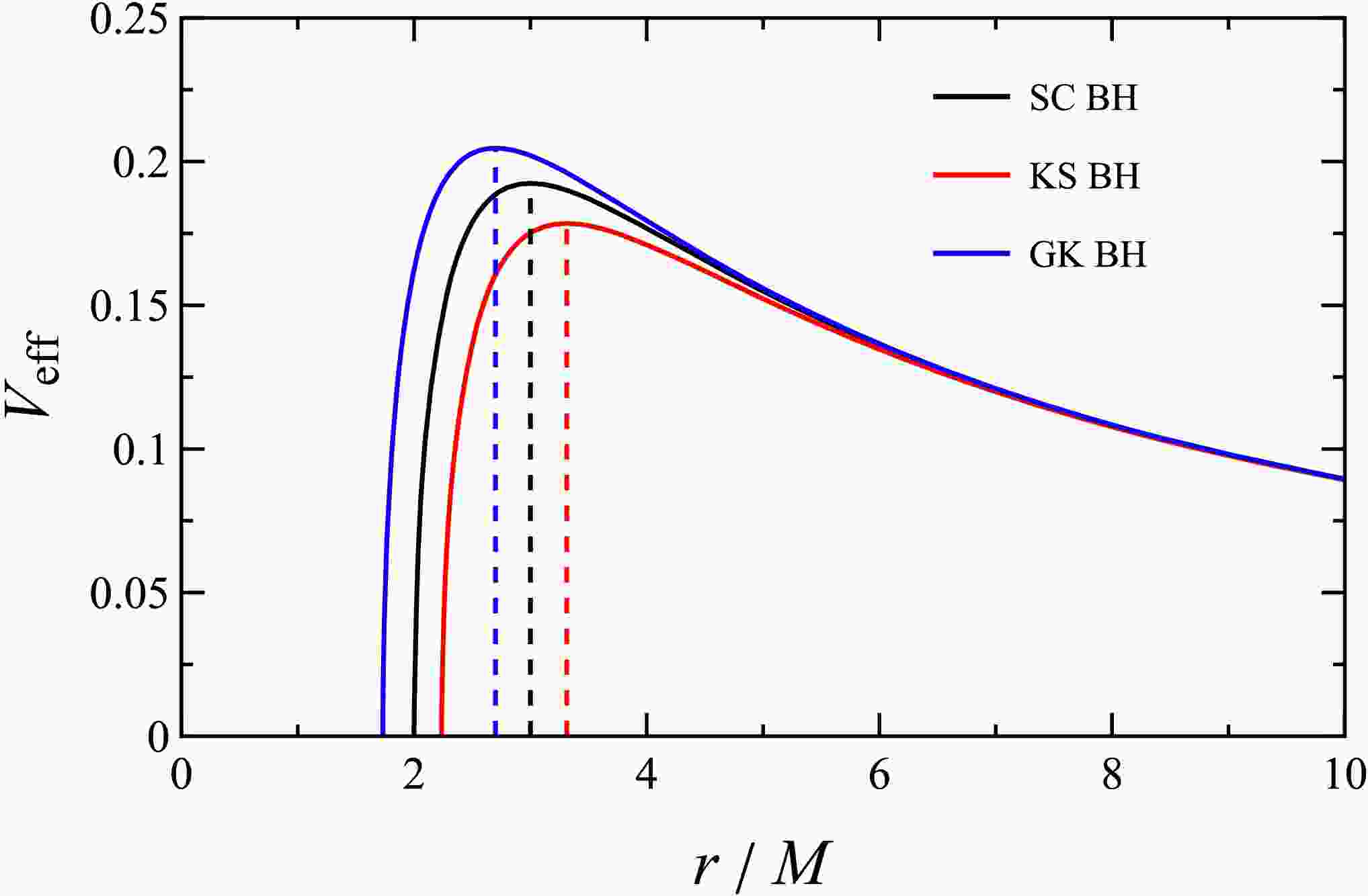
Fig. 1 depicts the effective potentials for the SC BH, as well as the KS BH with $ a^{{\rm{KS}}}/M=1 $ and GK BH with $ a^{{\rm{GK}}}/M=1 $. As shown in the figure, the three effective potentials start from zero at the event horizon ($ f(r_{h}) = 0 $), increase rapidly to a maximum as r increases, and then gradually decrease, approaching the same asymptotic value. Relative to the SC BH, the parameter $ a^{{\rm{KS}}} $ lowers the effective potential of the KS BH, indicating that photons require less energy to escape the BH. In contrast, the parameter $ a^{{\rm{GK}}} $ raises the potential for the GK BH, implying that photons need more energy to escape the BH. At the extrema $ r_p $ of the effective potential, the KS BH has a larger $ r_p $ than the SC BH, whereas the GK BH has a smaller $ r_p $. The extremum $ r_p $ of the effective potential $ V_{{\rm{eff}}} $ gives the radius of the photon sphere. The photon-sphere radius of the BH can be obtained by setting $ \partial V_{{\rm{eff}}}/\partial r=0 $. To investigate the effects of the "hair" parameters of various minimally deformed SC BHs on photon spheres and shadows, we set the BH mass to $ M=1 $. The corresponding photon-sphere radii for the three BHs are thus: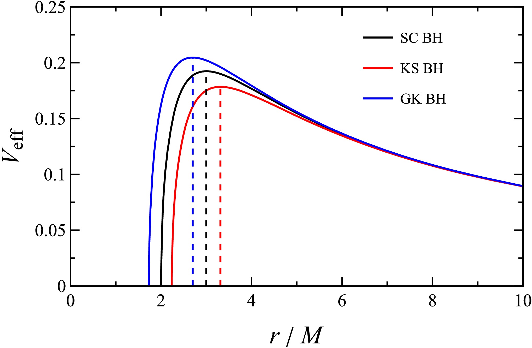

Figure 1.  (color online) The effective potential $ V_{{\rm{eff}}} $ is shown as a function of the radial coordinate r for three BHs. The black, red, and blue solid lines correspond, respectively, to the SC BH, the KS BH with $ {a^{{\rm{KS}}}}/M=1 $, and the GK BH with $ {a^{{\rm{GK}}}}/M=1 $.

● SC BH

● KS BH

● GK BH

where

Substituting Eqs. (31), (32), and (33) into $ b_p=1/ $ $ V_{{\rm{eff}}}(r_p) $ yields the critical impact parameters $ b_p $ for the three BHs as follows:

● SC BH

● KS BH

● GK BH

Fig. 2 presents the dependence of the photon sphere radius $ r_p $ and the critical impact parameter $ b_p $ on the minimum deformation parameters $ {a^{{\rm{KS}}}/M} $ and $ {a^{{\rm{GK}}}/M} $ for the two deformations of the SC BH. In the left panel, as either $ {a^{{\rm{KS}}}/M} $ or $ {a^{{\rm{GK}}}/M} $ increases from 0, the photon sphere radius of the KS BH increases rapidly relative to that of the SC BH, whereas that of the GK BH decreases, vanishing at $ {a^{\rm{GK}}/M=2} $. This indicates that increasing the magnetic charge $ {a^{{\rm{GK}}}/M} $ in the GK BH produces extremal BHs or naked singularities, which do not support photon spheres and thus cast no shadows. In the right panel, the latest EHT observations of Sgr A* [22, 39] constrain the parameters of the KS and GK BHs. The constraints from Keck and VLTI are as follows: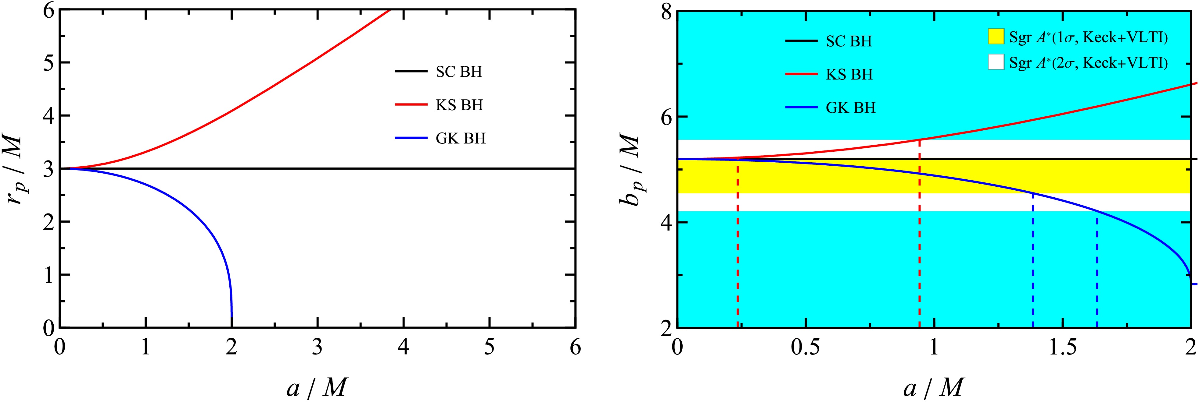

Figure 2.  (color online) Left panel: Dependence of the photon sphere radius $ r_p/M $ on the BH hair $ {a^{{\rm{KS}}}/M} $ and $ {a^{{\rm{GK}}}/M} $. As the parameters $ {a^{{\rm{KS}}}/M} $ and $ {a^{{\rm{GK}}}/M} $ increase, the photon sphere radius of the KS BH increases rapidly, whereas that of the GK BH decreases more rapidly, with the photon sphere disappearing at $ {a^{{\rm{GK}}}}=2M $. Right panel: Dependence of the critical impact parameter $ b_p/M $ on the BH hair $ {a^{{\rm{KS}}}/M} $ and $ {a^{{\rm{GK}}}/M} $. Using the average of the Keck and VLTI mass-to-distance ratio priors for Sgr A*, the yellow and white regions are consistent with the EHT angular size images of Sgr A* at the $ 1\sigma $ and $ 2\sigma $ levels, respectively. In contrast, the cyan region is excluded by the same observations at more than $ 2\sigma $ significance.

This yields the upper limits $ {a^{\rm{KS}}}/M\lesssim0.23 $ ($ 1\sigma $) and $ {a^{\rm{KS}}}/M\lesssim0.94 $ ($ 2\sigma $) for the KS BH, and $ {a^{\rm{GK}}}/M\lesssim1.38 $ ($ 1\sigma $) and $ {a^{\rm{GK}}}/M\lesssim1.63 $ ($ 2\sigma $) for the GK BH. Consistently, the EHT data strongly constrain theories in which the critical impact parameters increase with $ {a^{{\rm{KS}}}/M} $ and $ {a^{{\rm{GK}}}/M} $ [39]. It should be emphasized that the constrained upper limits on $ a^{\rm{GK}}/M $ are significantly lower than the extremal limit of the GK BH solution ($ a^{\rm{GK}}/M=2 $). All parameter values within the $ 1\sigma $ and $ 2\sigma $ constrained ranges admit complete event horizons, are physically self-consistent, and do not degenerate into extremal BHs or naked singularities. This ensures that all the solutions studied in this paper satisfy the physical premise of BH shadow formation.

Given the monotonic relationships between event horizons, photon-sphere radii, critical impact parameters, and BH "hair" parameters for KS and GK BHs, we fix $ {a^{{\rm{KS}}}/M=1} $ and $ {a^{{\rm{GK}}}/M=1} $ in both hairy BHs to explore their physical differences from the SC BH.

We then focus on photon trajectories. Taking the square root of Eq. (25) and multiplying by $ {\rm{d}}\lambda/{\rm{d}}\varphi $, we obtain the ray-trajectory equation

The positive or negative sign in the equation above depends on both the direction of light deflection and the variation of the radial coordinate. By introducing the new variable $ u\equiv1/r $, Eq. (37) can be transformed into

where the negative (positive) sign in this equation corresponds to the positive (negative) sign in Eq. (37). For the three BHs under consideration, the differential equations governing the ray trajectories are:

● SC BH

● KS BH

● GK BH

Fig. 3 shows ray trajectories, computed with a ray-tracing code, for the SC BH, the KS BH with $ {a^{{\rm{KS}}}}/M=1 $, and the GK BH with $ {a^{{\rm{GK}}}}/M=1 $. It is evident that even a minimal deviation from the SC BH endows the BH with "hair," thereby modifying the event horizon and photon sphere. As concluded previously, relative to the SC BH, the event-horizon and photon-sphere radii increase for the KS BH, but decrease for the GK BH. The weaker gravitational field of the KS BH results in smaller light deflection, whereas the magnetic charge of the GK BH strengthens the field, yielding more pronounced light deflection.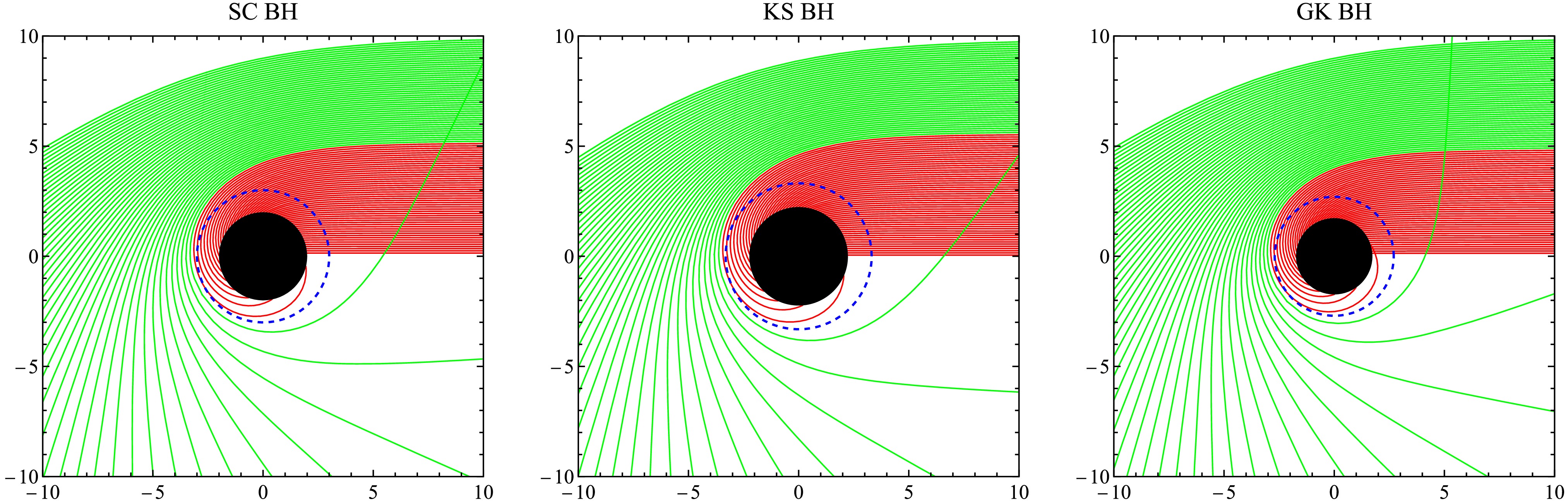

Figure 3.  (color online) Photon trajectories in the equatorial plane for three BHs. From left to right: SC BH, KS BH with $ {a^{{\rm{KS}}}}/M=1 $, and GK BH with $ {a^{{\rm{GK}}}}/M=1 $. In each panel, the red and green lines represent light rays with $ b<b_p $ and $ b>b_p $, respectively, while the blue dashed line denotes the photon sphere. Each BH is depicted as a black disk. Coordinates are scaled by M.

According to the no-hair theorem, black hole (BH) properties are uniquely determined by mass, charge, and angular momentum [74, 75]. However, the regular KS and GK BHs violate the dominant energy condition, placing them beyond the scope of the classical no-hair theorem. These solutions not only resolve the central singularity but also demonstrate that BH shadow formation depends sensitively on the "hair" parameters $ {a^{{\rm{KS}}}} $ and $ {a^{{\rm{GK}}}} $. In particular, the KS BH's shadow expands due to enhanced photon capture, whereas the GK BH's shadow contracts under the same conditions.

Matter in the universe, including plasmas, gases, and dust, generally moves freely. As it approaches a BH, this matter is drawn in by gravity and gradually accretes, forming an accretion flow. The accreting matter emits radiation, enabling observers to detect optical phenomena such as BH shadows and photon rings. By examining the characteristics of BH shadows and photon rings for different types of spherical accretion (static and infalling), we aim to gain a deeper understanding of how accretion influences the optical manifestations of BHs and to further explore BH properties. In this section, assuming luminous matter permeates the universe, we analyze how BH shadow size, brightness, and photon ring morphology depend on BH type and on the kinematic properties of the accreting matter under these scenarios.

We consider an optically thin, spherically symmetric accretion flow outside the BH event horizon, either statically distributed or infalling. The specific intensity $ I_{{\rm{obs}}}(b, \nu_o) $ measured by an observer at frequency $ \nu_{o} $ can be written as [51, 76−78]

Here, g denotes the ratio of the photon frequency measured by an observer at infinity, $ \nu_o $, to that measured by a static observer at the accretion region, $ \nu_e $ (i.e., $ g:=\nu_o/\nu_e $), and is referred to as the redshift factor. Moreover, $ j(\nu_{e}) $ is the emissivity per unit volume at frequency $ \nu_e $ as measured by a static observer at the location of the accreting matter, and $ {\rm{d}}l $ is the proper distance along the null geodesic in the accretion flow's reference frame. Finally, since the accretion flow extends to infinity, the integration path "ray" denotes the entire trajectory of light. The integrated intensity is obtained by integrating the specific intensity over all frequencies [57, 79].

We consider a simplified monochromatic emission scenario, as in Ref. [51], in which the emissivity follows a $ 1/r^2 $ radial profile and the rest-frame frequency is ν, i.e.,

Let $ Z^\mu $ denote the four-velocity of the accreting matter, and let $ U^\mu=(1,0,0,0) $ denote that of a static observer at infinity. In the case of static accretion, one finds

Thus, imposing the constraint $ g_{\mu\nu}Z^\mu Z^\nu=-1 $ on the 4-velocity of the accreting matter in the free-fall case, we obtain

where the negative sign of the radial coordinate in the above equation reflects that the accreting matter is approaching the BH. Here, $ \mathscr{E} $ is the conserved energy along the geodesic of the accreting matter, given by $ \mathscr{E}=-g_{\mu\nu}Z^\mu \xi_1^\nu $, and is determined by the initial rest position at the onset of infall. If the accreting matter begins to fall from rest at $ r = r_f $, the components of $ Z^\mu $ at that instant are $ (1/\sqrt{f(r_f)},0,0,0) $, so that $ \mathscr{E}=\sqrt{f(r_f)} $. The redshift factor g can be expressed as

Here, the subscript "obs" denotes the observation point in spacetime, whereas "em" denotes the photon-emission point in the accreting matter. Finally, the proper distance $ {\rm{d}}l $ is defined as [54, 76, 77]

Using Eqs. (24), (42), (43), (44), (45), (47), and (48), the integrated intensity in static spherical accretion is given by:

The integrated intensities for the three BHs are as follows.

● SC BH

● KS BH

● GK BH

Fig. 4 shows the distribution of the integrated intensity $ F_{{\rm{obs}}} $ versus the impact parameter b for three BHs, where the parameters of both KS and GK BHs are $ a^{\rm{KS}}/M=1 $ and $ a^{\rm{GK}}/M=1 $. It can be seen that the integrated intensities for all three BHs rise rapidly from a finite value, indicating that the shadow possesses nonzero intensity. Upon reaching the extremum, the intensities suddenly drop and then slowly decrease, tending toward the same value. Compared with the SC BH, the impact parameter corresponding to the peak integrated intensity of the KS BH is larger than the critical impact parameter of the SC BH. On the left, the integrated intensity is generally smaller than that of the SC BH, whereas on the right it is initially larger than that of the SC BH and finally tends toward the same value. In contrast, the impact parameter corresponding to the peak integrated intensity of the GK BH is smaller than that of the SC BH. On the left, the integrated intensity is larger than that of the SC BH, but on the right it is initially smaller than that of the SC BH and finally tends toward the same value. Crucially, the impact parameter that maximizes the integrated intensity always coincides with the critical impact parameter $ b_p $, implying that the photon ring radius equals $ b_p $.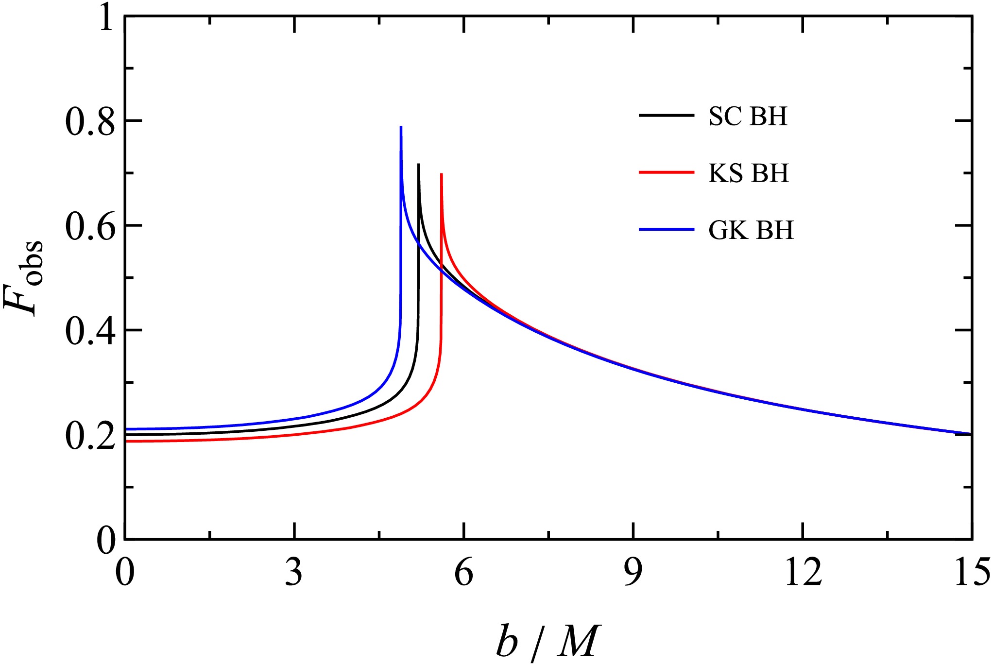

Figure 4.  (color online) The distribution of the integrated intensity $ F_{{\rm{obs}}} $ as a function of the impact parameter b is shown for three BHs undergoing static spherical accretion. The black, red, and blue solid lines correspond, respectively, to the SC BH; the KS BH with $ {a^{\rm{KS}}}/M=1 $; and the GK BH with $ {a^{\rm{GK}}}/M=1 $. For each BH, the integrated intensity attains its maximum at the critical impact parameter $ b_p $.

It is not difficult to understand the cause of this behavior. As is well known, the shadow of the GK BH contracts as magnetic charge increases, a consequence of the strengthened gravitational field. For small $ b/M $, gravitational lensing near the BH produces multiple light paths, enhancing the integrated intensity. At large $ b/M $, however, the strengthened gravitational field reduces the photon-sphere radius $ r_p $, thereby shrinking the angular size of the shadow. Consequently, a fixed impact parameter $ b/M $ corresponds to a larger angular offset from the shadow edge, placing the region farther from the strong-lensing zone and thus reducing the integrated intensity. For the same reason, quantum corrections cause the KS BH to exhibit the opposite trend to the GK BH.

Based on the integrated intensity distribution in Fig. 4, Fig. 5 displays optical images of the SC BH, the KS BH with $ {a^{\rm{KS}}}/M=1 $, and the GK BH with $ {a^{\rm{GK}}}/M=1 $. Compared with the SC BH, the KS BH exhibits a larger photon-ring radius and a lower shadow intensity, whereas the GK BH exhibits a smaller photon-ring radius and a higher shadow intensity. The origins of these imaging differences have been carefully analyzed in the preceding sections.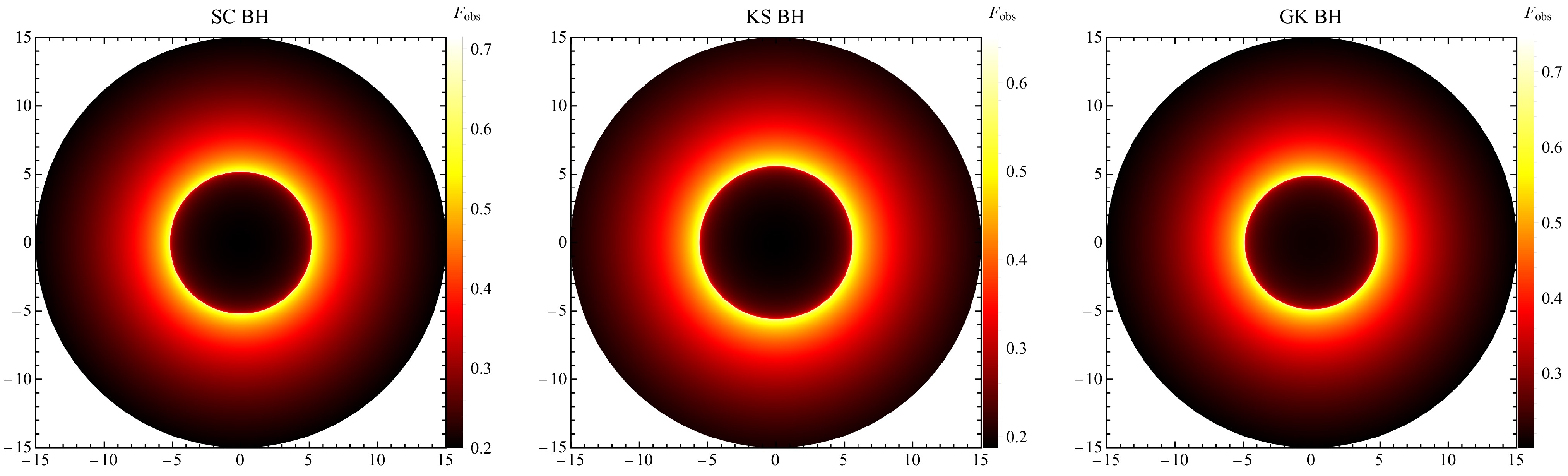

Figure 5.  (color online) Optical images of BHs under steady, spherically symmetric accretion. From left to right are the SC BH, the KS BH with $ {a^{\rm{KS}}}/M=1 $, and the GK BH with $ {a^{\rm{GK}}}/M=1 $. The integrated intensity for each color is shown by the color bar on the right of each panel, and the coordinate axes are labeled in units of the impact parameter $ b/M $.

By combining Eqs. (46) and (47) and imposing the condition $ \mathscr{E}=1 $ for matter radially infalling from infinity, we obtain an expression for the redshift factor for spherically symmetric radial infall.

In the equation above, the "+" sign denotes light rays moving away from the BH, whereas the "-" sign denotes light rays moving toward the BH. For the three BH types under discussion, the expressions for $ g_\pm $ are as follows:

● SC BH

● KS BH

● GK BH

Using Eqs. (24), (42), (43), (44), and (48), the integrated intensity for infalling spherical accretion can be derived as follows:

Substituting Eqs. (54), (55), and (56) into Eq. (57) yields the integrated intensity for infalling spherical accretion. Fig. 6 shows the dependence of the integrated intensity $ F_{{\rm{obs}}} $ on the impact parameter b for three BHs undergoing infalling spherical accretion. Compared with Fig. 4, the trends of the integrated intensity in the infalling and static accretion cases are similar, but the shadow intensity is significantly lower in the infalling case. The extremum of each curve likewise occurs at the critical impact parameter $ b=b_p $. The integrated intensities of the three BHs converge to similar values on the left side of $ b_p $. Compared with the static model, the integrated intensity in the infalling accretion model rises more rapidly to its maximum near $ b_p $. This implies a greater intensity contrast across the shadow boundary in the infalling accretion model than in the static accretion model. Similarly, relative to the SC BH, the KS BH has a larger photon ring, whereas the GK BH has a smaller one.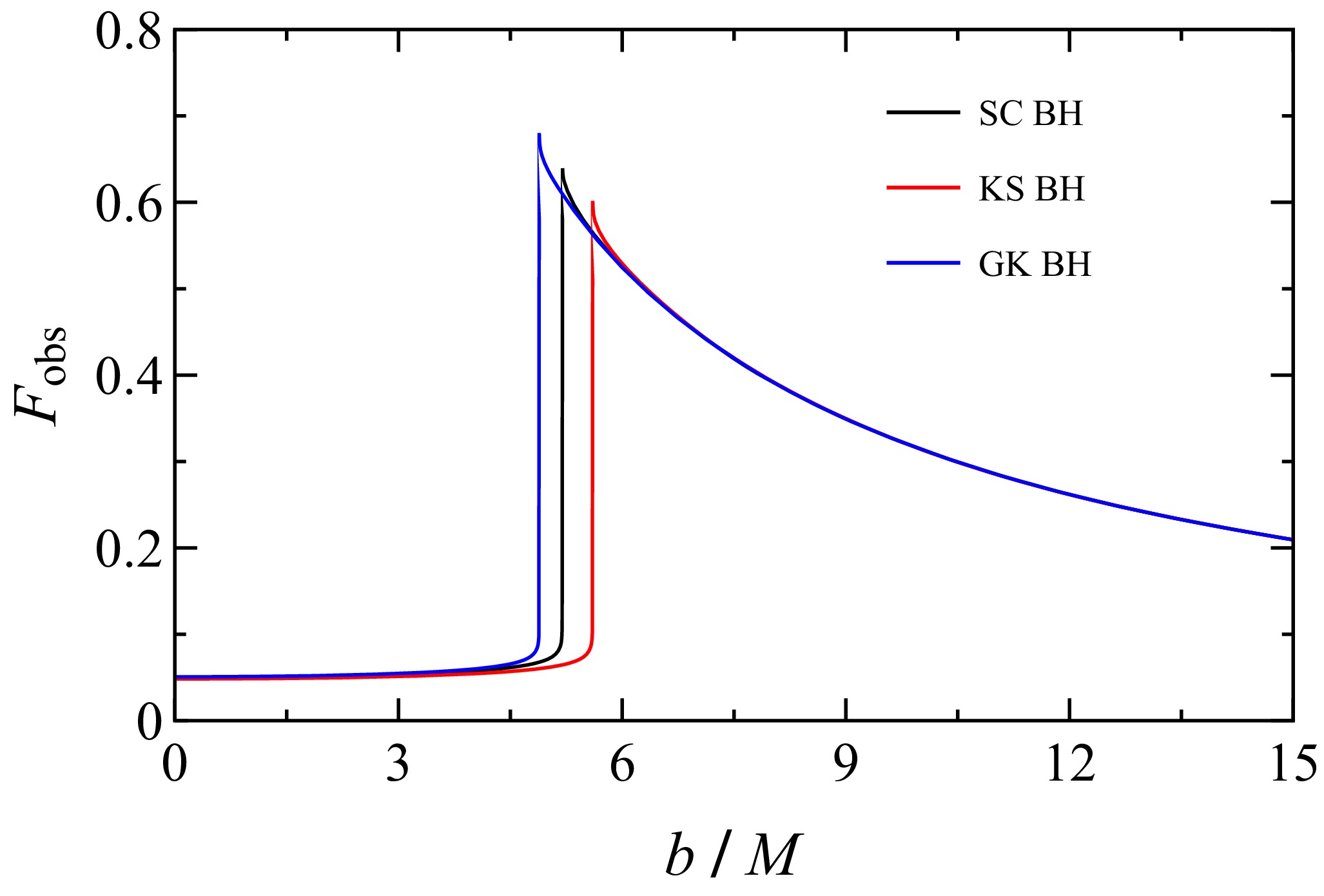

Figure 6.  (color online) Shown are the distributions of the integrated intensity $ F_{{\rm{obs}}} $ as a function of the impact parameter b for three BHs undergoing spherical infall accretion. The black, red, and blue solid lines correspond, respectively, to the SC BH, the KS BH with $ {a^{\rm{KS}}}/M=1 $, and the GK BH with $ {a^{\rm{GK}}}/M=1 $. For each BH, the maximum value of $ F_{{\rm{obs}}} $ occurs at the critical impact parameter $ b_p $.

Analogously to Fig. 6, the optical images of the SC BH, the KS BH with $ {a^{\rm{KS}}}/M=1 $, and the GK BH with $ {a^{\rm{GK}}}/M=1 $ are shown in Fig. 7. Clearly, the central low-intensity region corresponds to the shadow, surrounded by a bright photon ring. As previously discussed, for BHs with identical parameters, the integrated intensity at the shadow in the static-accretion case is significantly higher than in the infalling-accretion case, making the latter shadow darker. This behavior arises from Doppler redshift: the bulk infall velocity of the accreting matter is antiparallel to the photon propagation direction. Furthermore, for both minimal deformations of the SC BH, the shadow radius under spherical accretion equals the critical impact parameter $ b_p $, indicating that the observed shadow size is independent of the details of spherical accretion flows and is governed solely by the spacetime geometry.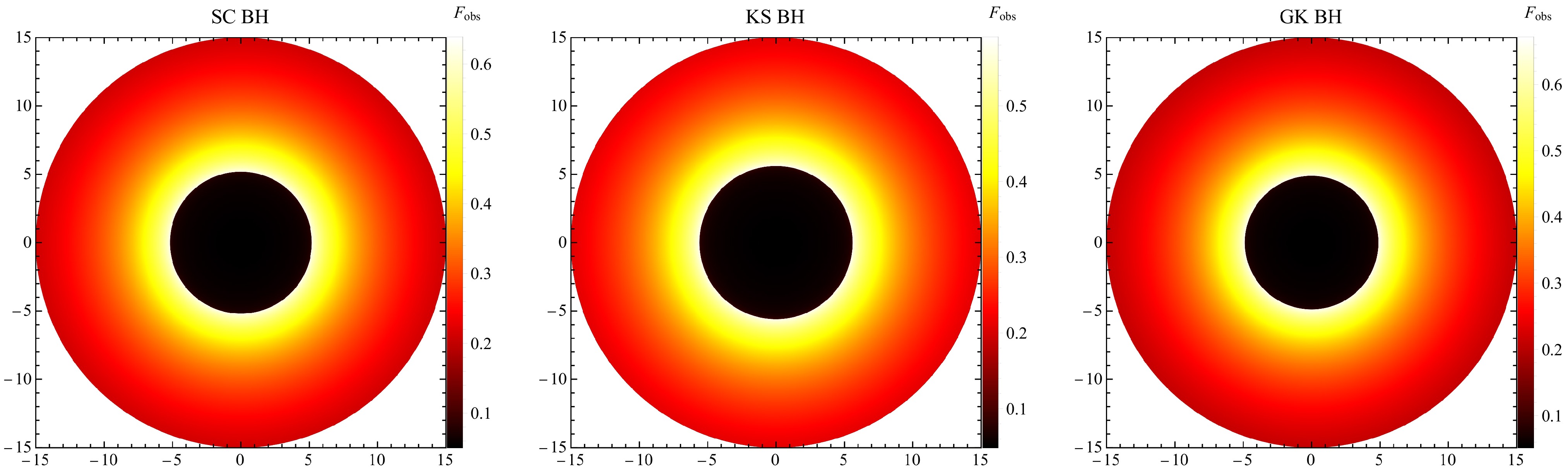

Figure 7.  (color online) Optical images of three BHs with spherically infalling accretion. From left to right, the panels show the SC BH, the KS BH with $ {a^{\rm{KS}}}/M=1 $, and the GK BH with $ {a^{\rm{GK}}}/M=1 $. The color scale at the right of each panel indicates the integrated intensity, and the axes are labeled by the impact parameter $ b/M $.

In this section, we discuss disk accretion, which is ubiquitous in the universe. In this framework, the disk-like accretion flow serves as the light source for the BH. We consider a static, optically thin, geometrically thin accretion disk in the equatorial plane, with the observer located directly above the disk. We will then discuss, in turn, the classification of light trajectories, the transfer function, and three specific thin-disk models to reveal the optical images of the thin disk for minimal deformations of the SC BH.

Light rays emitted by the disk-like accretion flow are deflected by the black hole (BH) due to its strong gravity, ultimately either being captured by the BH or escaping to infinity. Before reaching the observer, a ray may intersect the accretion disk multiple times. For a ray that intersects the disk k times, the azimuthal angle is $ \varphi=\pi/2+(k-1)\pi $. Therefore, the total number of photon orbits is

Building upon the classification framework pioneered by Gralla et al. [57], we adapt their criterion to categorize photons emitted from the thin accretion disk into three observable types according to the orbit number n, with specific modifications to the direct-emission classification. Specifically,

● When $ 0.25<n<0.75 $, the light ray intersects the accretion disk exactly once, which corresponds to direct emission.

● When $ 0.75<n<1.25 $, the light ray intersects the accretion disk twice, resulting in lensed ring emission.

● For $ n>1.25 $, a light ray intersects the accretion disk at least three times, indicating photon ring emission.

Fig. 8 shows the relation between the total number of photon orbits, n, and the impact parameter, b, for the SC BH, the KS BH with $ {a^{\rm{KS}}}/M=1 $, and the GK BH with $ {a^{\rm{GK}}}/M=1 $. In each panel, the red, green, and blue lines correspond to direct emission, lensed ring emission, and photon ring emission, respectively. The critical impact parameter $ b_p $ corresponds to the peak of n: at this value, light rays pass closest to the photon sphere, where unstable circular orbits allow photons to complete multiple rotations around the BH. As the impact parameter increases from zero, the total number of orbits increases for $ b<b_p $, peaks at $ b=b_p $, and then decreases monotonically for $ b>b_p $, asymptotically approaching a constant value. Examining the ranges of b for direct emission, lensed-ring emission, and photon-ring emission listed in Table 1 shows that the widths of the lensed-ring and photon-ring emissions for the KS BH are slightly smaller than those for the SC BH, whereas those for the GK BH are slightly larger.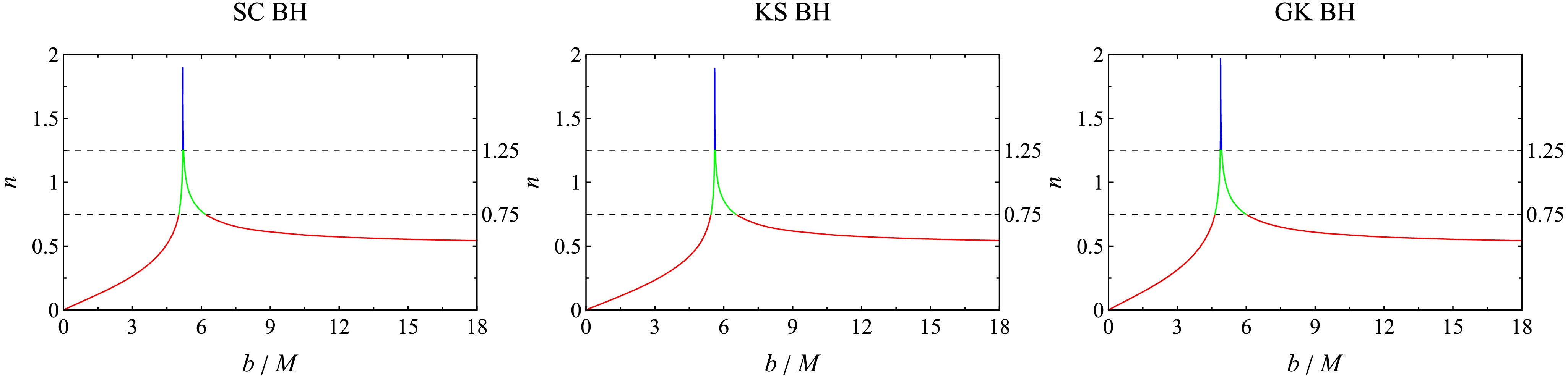

Figure 8.  (color online) Shown from left to right is the dependence of the total number of photon trajectories, n, on the impact parameter, b, for the SC BH, the KS BH with $ {a^{\rm{KS}}}/M=1 $, and the GK BH with $ {a^{\rm{GK}}}/M=1 $. The red, green, and blue lines correspond to direct emission, lensed-ring emission, and photon-ring emission, respectively.

Fig. 9 plots the light trajectories corresponding to different emission types for the SC BH, the KS BH with $ {a^{\rm{KS}}}/M=1 $, and the GK BH with $ {a^{\rm{GK}}}/M=1 $. Different colors denote distinct emission types. It should be noted that Fig. 9 is a refinement of Fig. 3. As shown, the KS BH exhibits a narrower range of lensed and photon rings, whereas the GK BH exhibits a broader range of such rings.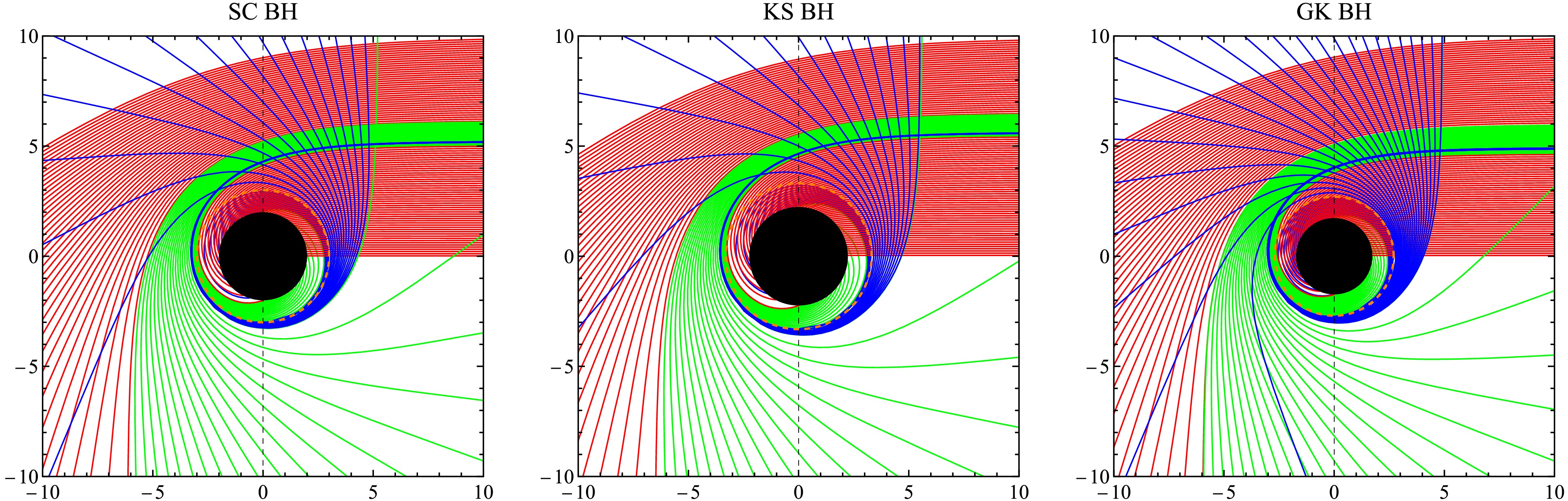

Figure 9.  (color online) From left to right, the behavior of different emission components of light around the SC BH, the KS BH with $ {a^{\rm{KS}}}/M=1 $, and the GK BH with $ {a^{\rm{GK}}}/M=1 $ is shown. Red lines correspond to direct emission, green to lensed-ring emission, and blue to photon-ring emission. The orange dashed line and the black disk denote the photon sphere and the BH, respectively, while the accretion disk is indicated by a black dashed line. Coordinates are scaled by M.

These results are intuitive. As discussed in Sec. III, introducing a magnetic charge endows the GK BH with a stronger gravitational field than the SC BH. Consequently, more light rays with impact parameters near the critical value $ b_p $ undergo larger deflections, producing broader lensed and photon rings. Conversely, due to quantum deformation, the KS BH exhibits a weaker gravitational field, resulting in fewer light rays experiencing large deflection angles near $ b_p $ and, hence, in narrower lensed and photon rings.

Let the specific intensity and frequency of the light emitted by the accretion flow be $ I_e(r) $ and $ \nu_e $, respectively. According to Liouville's theorem, $ I_e(r)/\nu_e^3 $ is conserved along the entire light path, so that $ I_e(r)/\nu_e^3=I_o(r)/\nu_o^3 $, where $ I_o(r) $ and $ \nu_o $ denote the specific intensity and frequency of the observed light, respectively. Using Eqs. (45) and (47), we obtain

To derive the integrated intensity, we integrate the observed specific intensity $ I_o(r) $ over the entire range of the photon frequency $ \nu_o $.

where $ I_{{\rm{emit}}} $ denotes the emitted specific intensity, defined as:

In the optically thin model, each intersection of a light ray with the accretion disk contributes to the specific intensity. Therefore, the integrated intensity, which is the sum of the incremental intensities accrued each time the light ray passes through the accretion disk, should be rewritten as

where $ r_k(b) $ denotes the transfer function [57], which relates the photon's impact parameter to the radial coordinate of the k-th intersection of the light ray with the accretion disk. This relation can be derived by integrating Eq. (38)

The slope of the transfer function, $ {\rm{d}}r_k(b)/{\rm{d}}b=\varGamma $, serves as the magnification factor and governs the angular demagnification. Fig. 10 shows the first three transfer functions for the SC BH, the KS BH with $ {a^{\rm{KS}}}/M=1 $, and the GK BH with $ {a^{\rm{GK}}}/M=1 $. The red line denotes the $ k=1 $ transfer function, corresponding to direct emission from the accretion disk. It is evident that the $ k=1 $ transfer functions for all three approximately follow a linear relationship with the impact parameter b ($ \varGamma\approx1 $), indicating that the direct emission traces the profile of a gravitationally redshifted source. Consistent with this, Fig. 10 shows that direct emission is the dominant component of the integrated intensity, accounting for the largest fraction of the radiation.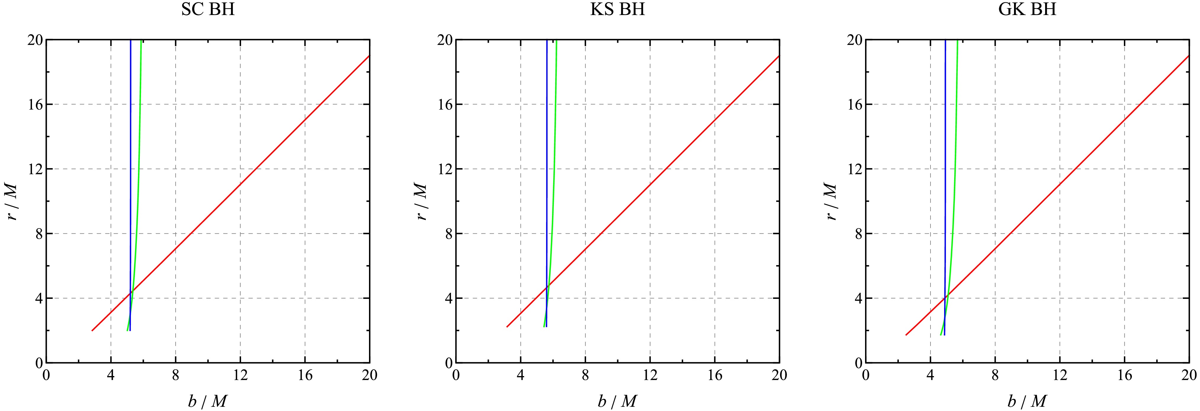

Figure 10.  (color online) Shown from left to right are the first three transfer functions for the SC BH, the KS BH with $ {a^{\rm{KS}}}/M=1 $, and the GK BH with $ {a^{\rm{GK}}}/M=1 $. The red, green, and blue solid lines represent the first, second, and third transfer functions, corresponding to direct emission, lensed ring emission, and photon ring emission, respectively.

The green line denotes the $ k=2 $ transfer function, corresponding to lensed-ring emission. Note that, regardless of whether the BH has 'hair', the slope of the second transfer function is extremely steep, indicating that the lensed image is highly demagnified. Finally, the blue line near $ b=b_p $ denotes the $ k=3 $ transfer function, corresponding to photon-ring emission. The slope of the third transfer function tends to infinity, implying that the photon-ring image is infinitely demagnified, rendering its flux effectively negligible.

We find that the shadow boundaries of all three BHs are determined by direct emission rather than by photon-ring or lensed-ring emission. In practice, only the first three transfer functions need to be considered, as higher-order emissions ($ k>3 $) contribute negligibly. These results are consistent with the discussion at the end of subsection 5.1. Notably, our findings are consistent with those reported by Gralla et al. [57].

In the thin-disk model, the accretion disk serves as the primary radiation source illuminating the BH. The emitted specific intensity of the accretion disk, $ I_{{\rm{emit}}}(r) $, depends not only on the radial emissivity profile but also on the location of the disk's inner edge, $ r_{{\rm{in}}} $. In this subsection, we analyze the optical properties of KS and GK BHs for three accretion disk emission profiles. For simplicity, we continue to assume monochromatic radiation.

● Model I: Starting from the Innermost Stable Circular Orbit

In the first model, the emission source region of the accretion disk begins at the radius of the innermost stable circular orbit (ISCO) for massive particles ($ r_{\rm{in}}=r_{\rm{ISCO}} $), and the emitted specific intensity is given by

where the radius of the ISCO, $ r_{{\rm{ISCO}}} $, is given by:

Here, $ f'(r) $ and $ f''(r) $ denote the first and second derivatives of $ f(r) $ with respect to r.

Fig. 11 shows the emitted specific intensity from the thin disk (first row), the integrated intensity (second row), and the corresponding BH images (third row) for the SC BH, the KS BH with $ {a^{\rm{KS}}}/M=1 $, and the GK BH with $ {a^{\rm{GK}}}/M=1 $ in the first model. It is evident that, compared with the SC BH, the ISCO radius $ r_{\rm{ISCO}} $ of the KS BH increases due to the presence of the parameter $ a^{\rm{KS}} $, whereas that of the GK BH decreases due to $ a^{\rm{GK}} $.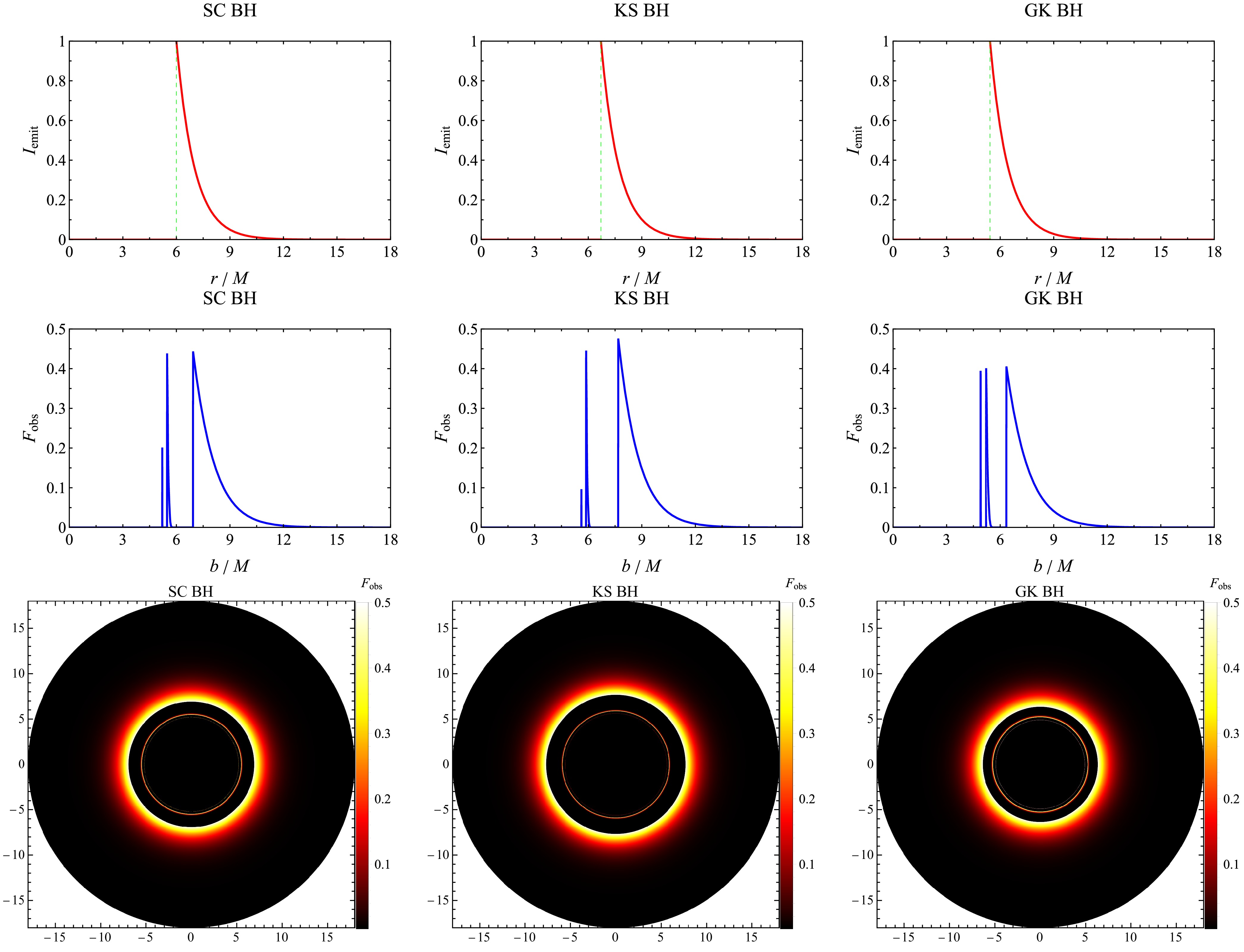

Figure 11.  (color online) In the first model, $ r_{{\rm{in}}} = r_{{\rm{ISCO}}} $. The first row shows the emitted specific intensity $ I_{\rm{emit}} $ of the thin accretion disk as a function of the radial coordinate r, the second row shows the observed integrated intensity $ I_{\rm{obs}} $ as a function of the impact parameter b, and the third row shows the optical appearance of the BH. From left to right, the columns correspond to the SC BH, the KS BH with $ {a^{\rm{KS}}}/M=1 $, and the GK BH with $ {a^{\rm{GK}}}/M=1 $. The coordinate axes are labeled by the impact parameter $ b/M $.

From the integrated intensity profiles of the three BHs, each exhibits three peaks. The first peak arises from photon-ring emission. Notably, the photon-ring intensity of the KS BH is lower ($ I_{\rm{obs}}\approx0.1 $), approximately half that of the SC BH, whereas the GK BH has a relatively higher photon-ring intensity, about twice that of the SC BH. The second peak in integrated intensity is produced by lensed-ring emission and shows little variation among the three, although that of the GK BH is clearly smaller than the other two. The third peak and the subsequent region are due to direct emission, which decays as b increases, following a trend similar to the emitted specific intensity $ I_{\rm{emit}} $. It is evident that the direct-emission peak of the KS BH is higher than that of the SC BH, while that of the GK BH is lower. These features are reflected in the images of the BHs in the third row. Moving from the outside to the inside of the black disk, a thin ring corresponds to the lensed ring. The photon ring appears inside the lensed ring but is nearly invisible because its extremely narrow width yields an extremely low flux (detectable only under strong magnification). With current observational capabilities, both the photon ring and the lensed ring are difficult to detect, so the observed shadow radius is primarily determined by direct emission.

In fact, due to the influence of different BH "hairs", the emission features of the three models are shifted relative to the SC BH: the KS BH shifts to the right (toward larger b), increasing the starting positions of the photon ring, lensed ring, and direct emission, whereas the GK BH shifts to the left (toward smaller b), decreasing the starting positions of the photon ring and lensed ring. Table 2 lists the initial positions of the photon ring, lensed ring, and direct emission for the three BHs in Model 1. From these data, the separations between the lensed ring and photon ring are similar among the three, but the separations from the photon ring to the onset of direct emission differ significantly. Thus, taking the distance between the lensed ring and photon ring $ B=b_{{\rm{L}}}-b_{{\rm{P}}} $ as a basic unit, the distance from the lensed ring to the onset of direct emission $ {\rm{\Delta}}b=b_{\rm{D}}-b_{{\rm{L}}} $ can be used to distinguish different types of BHs. Specifically, this method yields $ {\rm{\Delta}} b/B\approx5.41 $ for the SC BH, $ {\rm{\Delta}} b/B\approx6.92 $ for the KS BH, and $ {\rm{\Delta}} b/B\approx3.65 $ for the GK BH. These results show that $ {\rm{\Delta}} b/B $ is larger for the KS BH and smaller for the GK BH than for the SC BH.

In addition, it should be emphasized that this discriminant is established strictly at the theoretical level and depends on a specific accretion disk model. Given the angular resolution and observational uncertainties of the current EHT, the fine relative structure among the photon ring, lensed ring, and direct emission required by this method cannot yet be resolved in actual observations. This does not contradict the Kerr hypothesis supported by current EHT data. At the EHT’s observational precision, the detailed features of the lensed ring and photon ring are effectively lost, and the BH shadow is instead determined by direct emission.

● Model II: starting from the photon sphere

In the second model, the emission from the accretion disk begins at the radius of the unstable circular photon orbit ($ r_{\rm{in}}=r_p $), and the emitted specific intensity is given by

Analogously, Fig. 12 presents the observational features of the three BHs in the second model. As with $ r_{\rm{ISCO}} $, the $ r_p $ for the KS BH increases in the presence of the hair parameters $ a^{\rm{KS}} $ and $ a^{\rm{GK}} $, whereas that for the GK BH decreases, relative to the SC BH. The integrated intensity distributions of the three BHs consistently exhibit double-peaked profiles. The first peak arises from direct emission, and the second from the superposition of lensed-ring and photon-ring emissions, with little difference among the three. Relative to the SC BH, the KS BH shows higher intensity, whereas the GK BH shows lower intensity. In the BH images in the third row, the two brightest rings are visible: the innermost is produced by direct emission, and the outermost by the combination of lensed-ring and photon-ring emissions, which are difficult to distinguish in the figure. Regarding the shadow radius, that of the KS BH is larger than that of the SC BH; conversely, that of the GK BH is smaller. More importantly, the shadow radius in the second model is significantly smaller than in the first model, indicating that, in the thin-disk accretion model, the shadow radius is closely related to the details of the accretion flow.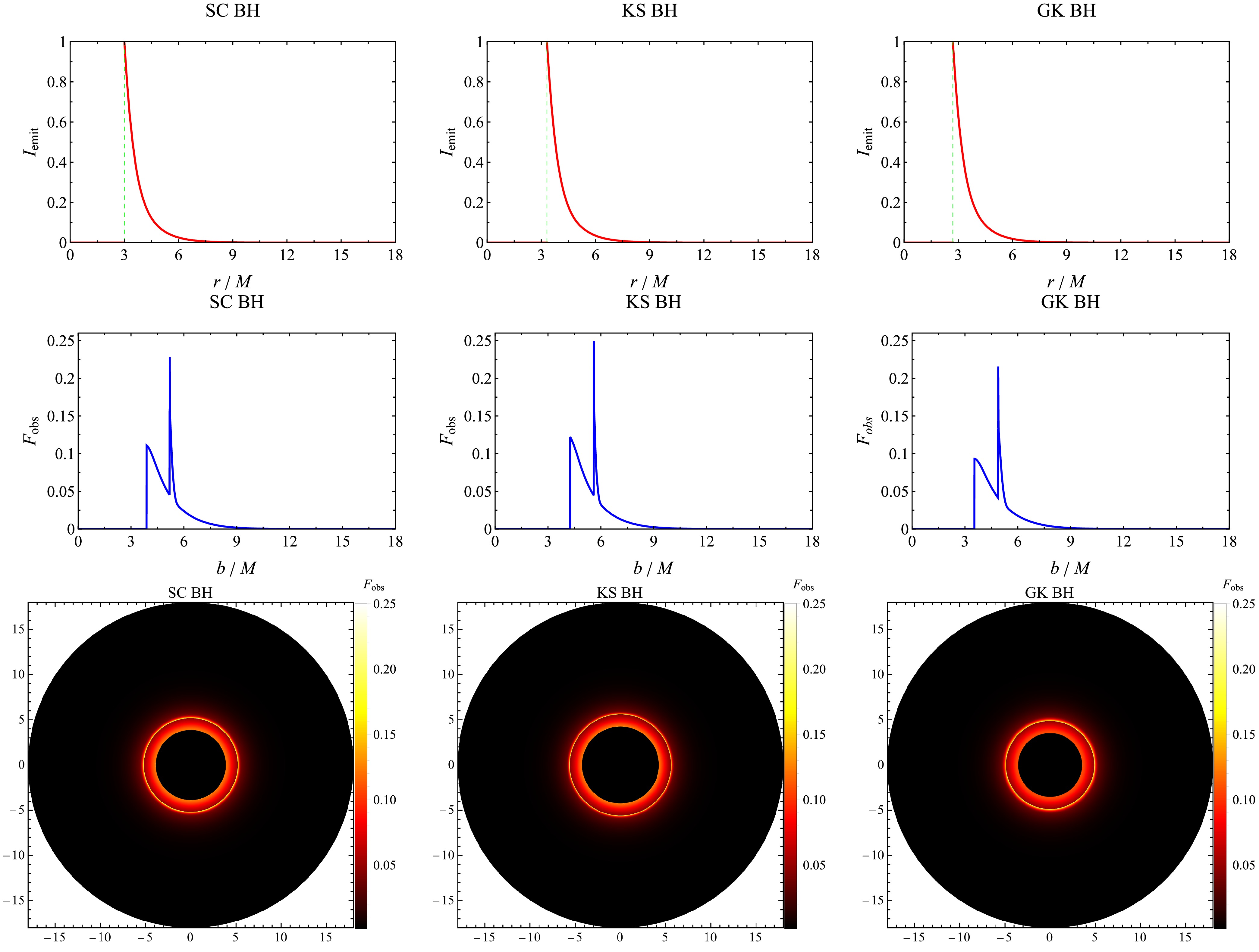

Figure 12.  (color online) As in Fig. 11, we use the second model ($ r_{\rm{in}}=r_p $).

● Model III: Starting from the Event Horizon

Finally, we consider a model in which the emitted specific intensity decays more gradually than in the first two models. The accretion-disk radiation originates at the event horizon $ r_h $, and its expression is given by

Fig. 13 presents the observational signatures of the different BHs in the third model. As with the ISCO ($ r_{\rm{ISCO}} $) and the radius of the unstable photon circular orbit ($ r_p $), the event-horizon radius ($ r_h $) of the KS BH increases relative to the SC BH owing to the hair parameter, whereas that of the GK BH decreases. In the integrated-intensity profiles (second row), all three BHs exhibit two closely spaced peaks. The first peak is primarily due to photon-ring emission. Although it coincides with the location of the maximum integrated intensity for all three BHs, its flux is much smaller than that in the neighboring regions dominated by lensed-ring and direct emission. The photon ring of the KS BH is brighter, while that of the GK BH is dimmer. The second peak arises primarily from the lensed ring. Overall, the KS BH is brighter than the SC BH, whereas the GK BH is dimmer. In the images shown in the third row, the shadow radius $ b_p $ for all three BHs slightly exceeds the critical impact parameter corresponding to the event horizon ($ b=r_h $). The bright ring outside the shadow contains contributions from both the photon ring and the lensed ring, which are difficult to distinguish because of their close proximity. The moderately bright region between the photon ring and the shadow arises from direct emission, indicating that, in this case, the shadow boundary is set by direct emission. Consequently, the shadow radius is smaller in this model.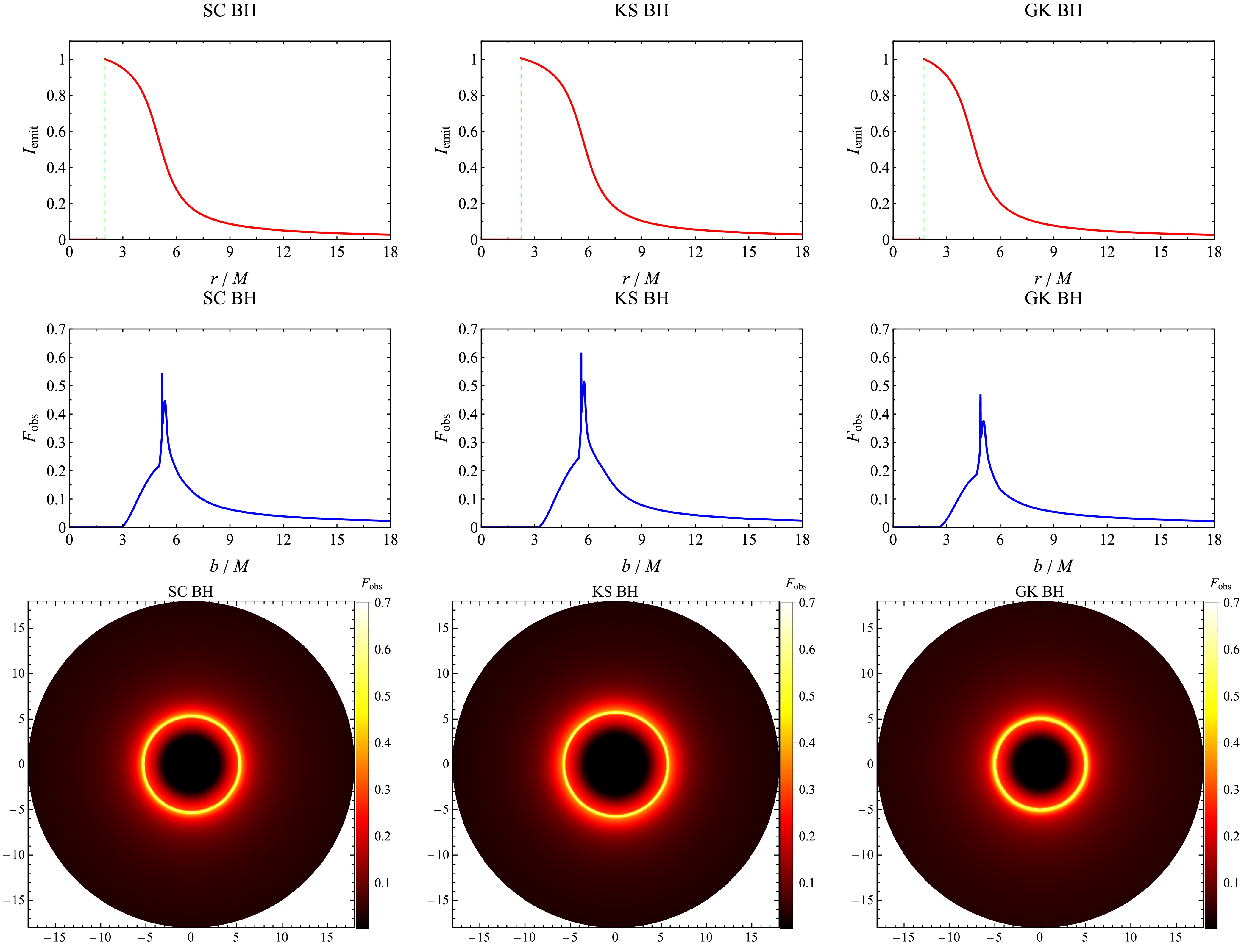

Figure 13.  (color online) As in Fig. 11, we adopt the third model ($ r_{\rm{in}}=r_h $).

Across the three models above, the contributions from photon-ring and lensed-ring emission are much smaller than those from direct emission; thus, direct emission dominates the total radiation intensity. In Sec. IV, we concluded that the observed shadow size is independent of the spherical accretion flow model; however, in disk models, different accretion prescriptions yield different shadow sizes. Specifically, from the first to the third models discussed in this subsection, the shadow radius decreases monotonically. The closer the accretion disk is to the BH, the smaller the onset radius of direct emission, and the smaller the shadow radius. In thin-disk models, the reason that the shadow sizes of different BHs within the same model differ is the same as in the spherical accretion model, and the spherical-accretion discussion applies directly to the thin-disk case.

This paper mainly studies the light trajectories, light intensity distributions, and optical appearances of two minimal deformations of the SC BH with spherical accretion and thin disk accretion, namely the KS BH and the GK BH, and discusses the deviations of them compared with the SC BH. Due to the minimal deformations, the radii of the event horizons, photon spheres, and shadows of the hairy BHs differ from those of the SC BH. Specifically, the KS BH has larger radius, but the GK BH has smaller radius. These results arise because the parameters of hairy BHs alter the gravitational effects of the BHs. Based on the shadow radius estimated by EHT, we obtained constraints on the hair parameter $ a^{\rm{KS}} $ and $ a^{\rm{GK}} $ for the two BHs. For the KS BH, the $ 1\sigma $ upper limit of the deformation radius $ a^{{\rm{KS}}} $ is approximately 0.23, and the $ 2\sigma $ upper limit is approximately 0.94. For the GK BH, the $ 1\sigma $ upper limit of the magnetic charge $ a^{{\rm{GK}}} $ is approximately 1.38, and the $ 2\sigma $ upper limit is approximately 1.63. These results can be employed to constrain the parameter selection of quantum deformations and the NED theory.

In the scenarios of two spherical accretion models, we obtain the distributions of integrated intensity for the two hairy BHs. The results show that, compared with SC BH, KS BH leads to shadow expansion and weakens the gravitational field due to quantum-corrections, but GK BH results in shadow contraction and strengthens the gravitational field due to the introduction of magnetic charge. Whether considering static spherical accretion or infalling spherical accretion, a stronger gravitational field leads to a brighter shadow. It is worth noting that the details of the two spherical accretion flows do not affect the shadow radius, but they have a significant impact on the integrated intensity of the shadow. Thus, the shadow radius is only related to the spacetime structure. Due to the Doppler effect, the shadow in the infalling spherical accretion scenario is obviously dimmer than that in the static spherical accretion scenario, and the intensity difference between the inside and outside of the shadow is larger.

In the three models of optically and geometrically thin accretion disks, we systematically investigated the observational features of these three types of BHs (SC, KS, and GK BHs). These results show that the optical appearances of all three BHs exhibit narrow photon rings, and that lensed rings exist outside the photon rings. Compared with the SC BH, the widths of the lensed and photon rings for the KS BH are narrower due to quantum-corrections, while those for the GK BH are broader due to the introduction of magnetic charge. In addition, the dominant contribution to the observed integrated intensity originates from direct emission, with negligible contributions from photon and lensed rings. Notably, distinct from spherical accretion, the boundary of the observed BH shadow in disk accretion is not determined by the critical impact parameter, photon ring, or lensed ring, but by direct emission. Overall, among the three models, the KS BH exhibits the highest brightness, but the GK BH exhibits the lowest dimness. In the first model, we propose a method to distinguish among the three BHs, which can aid in testing GR and other gravitational theories.

It should be emphasized that the research in this paper still has certain limitations in the context of current astronomical observations. On the one hand, the current EHT observations of Sgr A* and M87* strongly support the Kerr hypothesis, that is, the observed supermassive BHs can be fully described by the Kerr solution (SC solution for the spinless case) within the observational uncertainty. When the deformation parameters $ a^{\rm{KS}} $ and $ a^{\rm{GK}} $ are within the $ 1\sigma $ constraint range given by EHT in this paper, the shadow radius of KS and GK BHs are highly consistent with that of the SC BH, showing significant parameter degeneracy. On the other hand, the discrimination method for different BHs proposed in this paper relies on the measurement of the relative position of the photon ring and lensed ring, whose angular scale is far below the angular resolution limit of the current EHT. Therefore, this method is only theoretically feasible at present, and cannot be directly applied to actual astronomical observations with existing equipment.

Nevertheless, the theoretical discrimination criterion proposed in this paper still has important scientific value. With the upgrading of the next-generation EHT and the development of space very long baseline interferometry technology, the angular resolution of BH imaging will be greatly improved in the future. At that time, the method proposed in this paper can be used to test the general relativity, and search for the quantum correction effects or nonlinear electrodynamics effects in the strong gravitational field of BHs.

The conclusions of this paper are in good agreement with existing similar studies: For other quantum-corrected BHs such as 4D Gauss-Bonnet [55] (all of which are well-defined higher-derivative gravity theories that naturally emerge in UV-complete quantum gravity like string theory), they generally possess larger horizons and photon sphere radii than SC BHs, with an expanding trend in shadow size and higher shadow intensity in accretion disk models, consistent with the behavior of KS BHs in this paper. In contrast, Bardeen BH, Hayward BH [66], and Ayón-Beato-García BH coupled with a cloud of strings [80], those NED BHs carrying magnetic charge, exhibit smaller horizons and photon sphere radii than SC BHs, along with shrinking shadows and lower shadow intensity in disk models, aligning with the features of GK BHs discussed herein. The unified imaging framework established in this work can be directly extended to comparative studies of the aforementioned analogous BHs, which is one of the core directions of our subsequent research. In fact, we have already found that when only scale factors (e.g., event horizon, photon sphere, and photon ring radii) are considered, Einstein cubic gravity [81] and Einstein quartic gravity [82] yield results identical to KS BHs in this paper, while the standalone Ayón-Beato-García BH [83] and other NED [84] BHs also conform to the discussion of GK BHs here. Therefore, one of our future works is to demonstrate that these BHs are consistent with the results of this paper in terms of shadow intensity as well.

Code and software generated and/or analysed during the current study are available from the corresponding author upon reasonable request.

In Ref. [62], Kazakov and Solodukhin provided a detailed derivation of the reduction from the 4D Einstein–Hilbert action to the 2D effective dilaton action. We review this procedure in Appendix A. Kazakov and Solodukhin considered a decomposition of the metric $ g_{\mu\nu} $ into a spherically symmetric part $ g_{\mu\nu}^{{\rm{sph}}} $ and a non-spherical quantum fluctuation $ h_{\mu\nu} $, i.e.,

At leading order, the non-spherical fluctuations $ h_{\mu\nu} $ may be treated as classical fields.

The Einstein-Hilbert action is given by:

where G denotes Newton's gravitational constant (we refrain from using geometric units here) and g is the determinant of the metric $ g_{\mu\nu} $. We assume that, to leading order, both the 4D metric $ g_{\mu\nu} $ and the matter fields are spherically symmetric. Applying the coordinate transformation $ (t,r,\theta,\varphi)\mapsto(z^+,z^-,\theta,\varphi) $ to Eq. (1) yields

In the SC metric, $ z^+ $ and $ z^- $ serve as Kruskal coordinates. It can be shown that the Ricci scalar

has as its first term the Ricci scalar $ R^{(2)} $ of the 2D metric

namely,

where $ (\nabla r)^2=g^{(2)\alpha\beta}(\nabla_\alpha r)\nabla_\beta r $, $ \square=g^{(2)\alpha\beta}\nabla_\alpha\nabla_\beta $, and the indices $ \alpha,\beta $ take values 0 and 1. Here $ g^{(2)}_{\alpha\beta} $ is the 2D metric determined by $ ({\rm{d}}s^2)^{(2)} $. From Eq. (A3), we find $ g=({\rm{e}}^{2\sigma}r^4\sin^2\theta)/4 $, and thus the action can be rewritten as

where $ {\rm{d}}^2z={\rm{d}}z^+{\rm{d}}z^- $, and we have omitted the boundary term $ \square r^2 $.

Note that Eq. (A6) is a special case of 2D dilaton gravity [85−88]. By introducing the dilaton field $ \phi=\ln(r^2/G) $, Eq. (A6) can be cast into the form of a dilaton gravity action.

where $ U(\phi)=2/G $. Recognizing that quantum corrections will alter the form of the potential $ U(\phi) $, we introduce the dimensionless variable $ \xi=r/\sqrt{G} $ and generalize the preceding expression to an arbitrary dilaton potential, resulting in the generalized action

Equation (2) is presented below.

Varying the action with respect to the two-dimensional metric $ g^{(2)\alpha\beta} $ and the field ξ yields the equations of motion shown in Eq. (3).

Eq. (A9) implies the existence of a two-dimensional Killing vector field $ \xi_\alpha=\varepsilon_{\alpha\beta}\nabla^\beta\xi $ (where $ \varepsilon_{\alpha\beta} $ denotes the two-dimensional Levi-Civita symbol) that satisfies the Killing equation.

Thus, the field ξ may be chosen as a spacelike coordinate, thereby allowing $ ({\rm{d}}s^2)^{(2)} $ to be written as

This form satisfies the relations

where $ g^{(2)} $ denotes the determinant of the metric $ g^{(2)}_{\mu\nu} $. Substituting Eq. (A12) into Eq. (A9) yields

where the integral is taken to be indefinite, and the integration constant is omitted. Finally, reverting ξ to r and employing geometric units ($ G=1 $) gives

This is Eq. (9) in subsection II A; substituting it into Eq. (1) yields the 4D metric.