Solving the Inverse Source Problem in Femtoscopy with a Toy Model

As a residual force of QCD, hadron-hadron interactions play a significant role across various domains of particle physics, ranging from hadron structure and strong decays to weak decays of heavy-flavored hadrons. Recent studies on exotic states further highlight the importance of hadron-hadron interactions in understanding their properties, suggesting substantial molecular-hadronic components. Theoretical predictions for the ratios of strong decays $ {\cal{B}}[\psi(2S) \to \rho \pi] / {\cal{B}}[\psi(1S) \to \rho \pi] $ exhibit notable discrepancies with experimental data, a long-standing issue known as the "ρ–π puzzle" [1]. A conventional explanation attributes this puzzle to final-state interactions (FSIs), i.e., hadron-hadron interactions, considered essential for resolving the observed discrepancy [2−5]. FSIs also play a crucial role in the weak decays of heavy hadrons, significantly enhancing the branching fractions of nonfactorizable decays [6−12] and giving rise to substantial CP violation signals in these processes [13, 14]. Therefore, hadron-hadron interactions are an essential input for phenomenological studies across particle physics, crucial for addressing problems associated with non-perturbative effects.

Currently, advances in lattice QCD have enabled detailed investigations of hadron–hadron interactions directly from first principles of QCD. In recent years, lattice QCD has successfully reproduced the nucleon–nucleon potential [15], demonstrating its capability to explore interactions between hadrons. Furthermore, invariant mass distributions are effective experimental observables for extracting information about hadron–hadron interactions. Cabibbo proposes a notable example to determine the $ \pi\pi $ scattering length from the $ \pi^0\pi^0 $ invariant mass distribution in the decay $ K^+ \to \pi^+\pi^0\pi^0 $ [16]. This is a method for determining dominant hadron-hadron interactions. Meanwhile, discoveries of exotic states in invariant-mass distributions shed light on interactions between nearby hadron pairs. Recently, femtoscopy, a technique that analyzes momentum correlations between particles produced in high-energy collisions, has emerged as a powerful alternative method for probing the strong interaction [17]. By measuring momentum-correlation functions (CFs), femtoscopy provides valuable insights into hadronic interactions. A particular strength of this approach lies in its ability to investigate hadron-hadron interactions involving unstable hadrons, which are not accessible via conventional scattering experiments [18−23]. This unique capability has stimulated significant theoretical developments [24−33].

The momentum CFs are described by the Koonin-Pratt (KP) formula [34, 35], which incorporates two essential components: 1) a particle-emitting source, characterizing the spatial distribution of hadron emission in relativistic heavy-ion collisions; 2) the scattering wave function, encoding the final-state interactions between hadron pairs. In general, the hadron-hadron interaction can be extracted from CFs using a known source function. Therefore, a precise source function is crucial for precisely extracting these interactions. The discussions on the particle-emitting source have been intensive [36−40]. Sources are often modeled as Gaussian functions. In this case, the characteristic source size produced in proton-proton collisions at LHC energies is about $ 1 $ fm [22], while $ 3-5 $ fm in nucleus-nucleus central collisions [18]. It is worth noting that an effective Gaussian source has been successfully applied in various experimental analyses [21, 22]. Alternatively, a Cauchy source has also been employed to characterize source functions. In a recent study, Wang et al. employed machine learning to extract the source function of the proton–proton system, using precise wave functions and experimental data [40]. However, the so-determined source function deviates from a Gaussian form. Indeed, the task of reconstructing source functions from experimental correlation data falls within the category of an "inverse problem", offering a novel perspective on extracting source functions.

The theory of inverse problems, a cornerstone of applied mathematics, provides a rigorous framework for reconstructing unknown quantities from indirect measurements and has been extensively applied in fields such as geophysical exploration and medical imaging [41]. The reconstruction of source distributions from measured correlation functions was pioneered by Brown and Danielewicz through the so-called image technique [42, 43]. This method employs optimized discretization to address the inherent instability of the inverse problem. The fundamental principle of the optimized discretization approach is to adjust the sizes of the radial bins $ r_{j} $ in order to minimize the relative error in the reconstructed source. Then motivated by the problem in optical imaging, Danielewicz et al., treat the imaging problem as an Optical Deblurring Problem solved via Bayesian Iteration [44, 45]. This iterative Bayesian method leverages the natural positivity of both the source and the kernel, and successfully incorporates detector resolution effects through convolution. While both methods have proven powerful, they rely on either optimized discretization strategies or iterative Bayesian frameworks. In this work, we explore an alternative path: we formulate the source reconstruction as a classical inverse problem and employ Tikhonov regularization, a mathematically rigorous technique that stabilizes the inversion through a penalty term ¹

This paper is structured as follows. Following the methodology of Ref. [64], we first generate momentum correlation functions from wave functions derived from a square-well potential with four distinct interaction strengths—repulsive, weakly attractive, moderately attractive, and strongly attractive. These are combined with Gaussian-type source functions and their mixtures. Subsequently, we attempt to reconstruct these source functions by solving the inverse problem, using the resampled correlation functions (with 1% and 10% uncertainties) along with the corresponding wave functions. Section II introduces the formalism for computing correlation functions using both a square-well potential and a Gaussian-type source function, as well as the approach to the inverse problem. Our numerical results and a detailed discussion are presented in Section III. Finally, we provide a summary and outlook in the last section.

Because current parameterizations of source functions rely on specific assumptions, it is essential to develop a model-independent approach to determine them. In this work, we propose a rigorous mathematical framework for computing source functions. Given momentum CFs and scattering wave functions, the source function can be reconstructed through an inverse problem. This section provides a concise introduction to the theoretical framework for momentum CFs and the inverse-problem approach.

The two-hadron momentum correlation functions (CFs) are computed using the KP formula [34, 35, 65].

where $ S_{12}(r) $ denotes the source function and $ \Psi^{(-)}(r,k) $ denotes the relative wave function, defined in the center-of-mass frame with relative coordinate r and relative momentum $ k=(m_2 p_1-m_1 p_2)/(m_1+m_2) $. The source function characterizes the spatial distribution of the emission source, and the wave function describes the final-state hadron-hadron interactions.

In what follows, we adopt a Gaussian form to represent the source function,

where R is the effective radius of the source.

The outgoing wave function of an S-wave interaction is generally expressed as [26]

where the Bessel function $ j_0 $ represents the $ l=0 $ orbital-angular-momentum component of the free wave function, whereas $ \psi_0 $ denotes the S-wave scattering wave function after the final-state-interaction correction. The scattering wave function has the following asymptotic behavior,

where δ denotes the phase shift. Finally, the momentum CFs are given by

In general, the scattering wave function can be obtained by solving the Schrödinger equation in coordinate space or the Lippmann-Schwinger equation in momentum space [24, 27, 66]. In what follows, we employ the Schrödinger equation to compute the scattering wave function. As indicated in Ref. [67], the off-shell ambiguity in strong interactions is generally associated with the short-distance behavior of relative wave functions, which can introduce theoretical uncertainties into calculations of CFs. Nevertheless, such off-shell ambiguities are not expected to be particularly significant in practice. Quantitative studies have shown that off-shell effects remain relatively mild in realistic interaction models of the two-body problem [68, 69]. Hence, while the off-shell ambiguity certainly exists, its impact on two-body systems is likely small. In our toy model, we assume the wave function is known a priori, so the issue raised in Ref. [67] does not arise.

Before detailing the methodology for inverse problems, it is useful to recall the notion of a forward problem. A forward problem consists of predicting outcomes from known causes using a given model. In contrast, an inverse problem aims to infer the causes from observed results and the model. As an illustration, the KP formula represents a forward problem: given the wave function and the source function, the correlation function is obtained via direct integration, which is generally straightforward. Conversely, the inverse problem of reconstructing the source function from the measured correlation function and the wave function is often challenging because it is typically ill-posed.

A central aspect of treating inverse problems is the study of their ill-posedness. Mathematically, a problem is termed well-posed if it satisfies three conditions simultaneously: existence, uniqueness, and stability of the solution [50, 51]. Existence requires at least one solution; uniqueness ensures at most one solution; and stability means that the solution depends continuously on the input data. If any of these three conditions is violated, the problem is ill-posed.

For a deterministic system in which the wave function is known precisely (e.g., the proton-proton system with accurately prescribed interactions), the inverse problem of extracting the source function from an experimentally measured correlation function is ill-posed. Specifically, it fails to satisfy the stability condition: an arbitrarily small perturbation in the input can produce arbitrarily large changes in the reconstructed source. To trace the origin of this instability, we discretize the KP equation using a rectangular quadrature rule, which leads to a linear algebraic system.

where the matrix $ K_{m\times n} $ is constructed from the values of $ \left| \Psi^{(-)} (r_i, k_j) \right|^2 $, and $ S_n $ and $ C_m $ denote the discretized source and correlation vectors, respectively. Here, n and m are the dimensions of these vectors. Performing a singular value decomposition (SVD) yields

where $ U = [u_1, \ldots, u_n] \in \mathbb{R}^{m \times n} $ and $ V = [v_1, \ldots, v_n] \in \mathbb{R}^{n \times n} $ contain orthonormal singular vectors ($ U^T U = V^T V = I_n $). The diagonal matrix $ \Sigma = {\rm{diag}}(\sigma_1, \ldots, \sigma_n) $ contains the singular values, ordered such that $ \sigma_1 \geq \cdots \geq \sigma_n \geq 0 $ [70]. The formal solution to $ C=KS $ is then

which is unique regardless of the relative sizes of m and n [70]. The numerical stability of the inversion is governed by the condition number $ \kappa(K)=\sigma_1/\sigma_n $. When $ \sigma_1 $ and $ \sigma_n $ differ by many orders of magnitude, the large condition number leads to severe numerical instability: high-frequency noise in the data is dramatically amplified in the reconstructed solution. Such ill-conditioning is inherent to the discretization of integral equations with smooth kernels: the resulting matrix K has rows (or columns) that are nearly linearly dependent, and this near-linear dependence forces the singular values to decay rapidly. Moreover, using SVD analysis, we quantify this instability.

where C denotes the exact data, $ S_t $ the corresponding true source function, and $ C^\epsilon=C+\epsilon $ the measured correlation function with error level $ \epsilon $. Here, $ \| \cdot \|_{l^2} $ is the standard $ l^2 $ norm on the sequence space, and $ S^\epsilon $ is the solution obtained from the noisy data. As the discretization is refined, the inverses of the singular values $ \sigma_i $ become unbounded.

The existence of a solution is often taken for granted based on the underlying physical picture. A rigorous uniqueness analysis of the inverse problem associated with the KP equation would require a functional-analytic framework, relying on an analytic kernel and continuous, noise-free data—conditions that are rarely met in practice. In particular, the matrix K may have a nontrivial null space, implying that certain components of the source function cannot be recovered without additional assumptions. Therefore, strict uniqueness cannot be guaranteed in the present setting. Nevertheless, it is common to assume that the corresponding continuous problem admits a unique solution [68, 69]. In this work, our goal is not to establish uniqueness rigorously, but to demonstrate the practical feasibility of reconstructing the source function from finite and noisy data [71, 72]. As shown in Sec. III, the reconstructed solutions capture the essential features of the exact source, indicating that the method is effective in practice even without guaranteed uniqueness. Thus, uniqueness is not the central limitation; rather, the main challenge is numerical instability, which persists even with large datasets or when the correlation function is treated as continuous.

To address this ill-posedness, regularization methods are employed. In mathematics, regularization refers to a family of techniques that transform an originally ill-posed problem into an approximately well-posed one, thereby ensuring the existence, uniqueness, and stability of an approximate solution [50, 51]. Although the use of "regularization" in physics—such as in the removal of divergences in loop integrals—differs in context from its mathematical counterpart for ill-posed inverse problems, both share the same essential objective: to achieve a well-defined and numerically stable formulation.

In this work, we employ the Tikhonov regularization scheme, a well-established approach that provides a rigorous framework for solving ill-posed inverse problems. The regularized solution $ S_\alpha^\epsilon $ is obtained by minimizing the Tikhonov functional

where $ \alpha>0 $ is the regularization parameter. This method, pioneered by Tikhonov, stabilizes the inversion by penalizing large oscillations in the solution. It underlies many contemporary regularization techniques used across diverse fields; see [54]. The first term enforces fidelity to the data $ C^\epsilon $, while the second term penalizes oscillations to stabilize the solution [56−58]. The matrix L encodes prior constraints on the solution, such as smoothness, positivity, or normalization; here, for simplicity, we choose a first-derivative operator to enforce smoothness, which suffices for the present analysis. Its discrete $ (n-1)\times n $ form is

Taking the variation of the Tikhonov functional yields

where $ \mathsf{T} $ denotes the matrix transpose. Eq. (12) illustrates how Tikhonov regularization stabilizes the inversion: the addition of $ \alpha L^\mathsf{T}L $ effectively reduces the condition number of the system. In particular, the regularized system maps $ \sigma_i $ to $ \sigma_i + \alpha $ (for an appropriate L), so that the original condition number $ \sigma_1/\sigma_n $ becomes $ (\sigma_1+\alpha)/(\sigma_n+\alpha) $.

This suppresses the amplification of noise in the small-singular-value directions and renders the problem well-posed.

A crucial aspect of Tikhonov regularization is the choice of the regularization parameter α. The Tikhonov functional makes explicit that the choice of α governs the trade-off between the fidelity term and the regularization term. If α is excessively large, the regularization term dominates, forcing the solution toward zero. Conversely, if α is too small, the fidelity term prevails and the inherent ill-posedness of the inverse problem re-emerges. Empirically, there is often a broad plateau with respect to α that aids robust selection. Numerous methods have been developed in inverse problems for determining the regularization parameter, including the L-curve criterion, the quasi-optimality criterion, and the discrepancy principle, among others [50, 51]. In this work, we employ the widely used L-curve criterion [73, 74], which exploits the trade-off between the residual $ \|K S_\alpha^\epsilon - C^\epsilon\|_{l^2} $ and the penalty $ \| L S_\alpha^\epsilon \|_{l^2} $: as α decreases, the residual decreases while the penalty increases. The L-curve is a log–log plot of these two quantities, and the optimal α is identified at its characteristic corner. This approach is fully deterministic and ensures that the inversion procedure involves no arbitrarily tuned parameters.

The reconstruction of the source function via Tikhonov regularization is governed by a rigorous mathematical framework that establishes two fundamental properties: numerical stability (well-posedness) and theoretical convergence. Specifically, as the noise level in the data tends to zero, the regularized solution $ S_\alpha^\epsilon $ converges to the true solution $ S_t $. This result can be stated as follows:

For a comprehensive theoretical treatment, including proofs of well-posedness and convergence, see Refs. [50−54].

In this section, we assess the performance of Tikhonov regularization for the inverse source problem in Femtoscopy using a toy model. We consider four distinct potential strengths and compute the corresponding wave functions by solving the Schrödinger equation. The true source functions $ S_t(r) $ are modeled in both single- and mixed-Gaussian forms. Using these wave functions and source functions, we calculate the correlation functions (CFs) $ C_t(k) $ via the Koonin-Pratt (KP) formula. Perturbed CFs $ C^\epsilon(k) $ are obtained by adding 10% and 1% random errors to $ C_t(k) $ to simulate realistic experimental uncertainties. This noisy $ C^\epsilon(k) $ then serves as input to Tikhonov regularization, which yields the reconstructed source function $ S^\epsilon_\alpha(r) $. Comparing $ S^\epsilon_\alpha(r) $ with the benchmark $ S_t(r) $ enables us to evaluate the effectiveness of Tikhonov regularization.

We now outline the potentials and source functions used in this work. We employ a square-well potential, chosen for its analytic wave function and its ability to capture generic features of the interaction through parameter adjustments. The potential is defined as:

where $ V_0 $ and d denote the strength and range of the potential, respectively. Following Ref. [64], we set the range parameter to $ d=2.5 {\rm{fm}} $ and take $ V_0 = 25, -10, -25, -75 {\rm{MeV}} $, corresponding to repulsive, weakly attractive, moderately attractive, and strongly attractive potentials, respectively.

The source functions fall into four types: the first two are single Gaussians, and the remaining two are Gaussian mixtures. This selection allows us to study both standard and more general source shapes. Explicitly, the sources are $ S_1(r,R) $ and $ S_2(r,R) $ (single Gaussians), and $ S_3(r,R) $ and $ S_4(r,R) $ (Gaussian mixtures of the form $ wS(r,R_1)+(1-w)S(r,R_2) $, where w is a weighting factor). The relevant parameter values are summarized in Table 1.

To numerically illustrate the inherent ill-posedness of reconstructing the source function from CFs, we begin by applying the standard SVD method given by Eq. (8) without regularization. As a representative case, we consider the potential $ V_0=-10 {\rm{MeV}} $ with a 1% uncertainty. Performing an SVD on the corresponding kernel matrix K yields the singular values

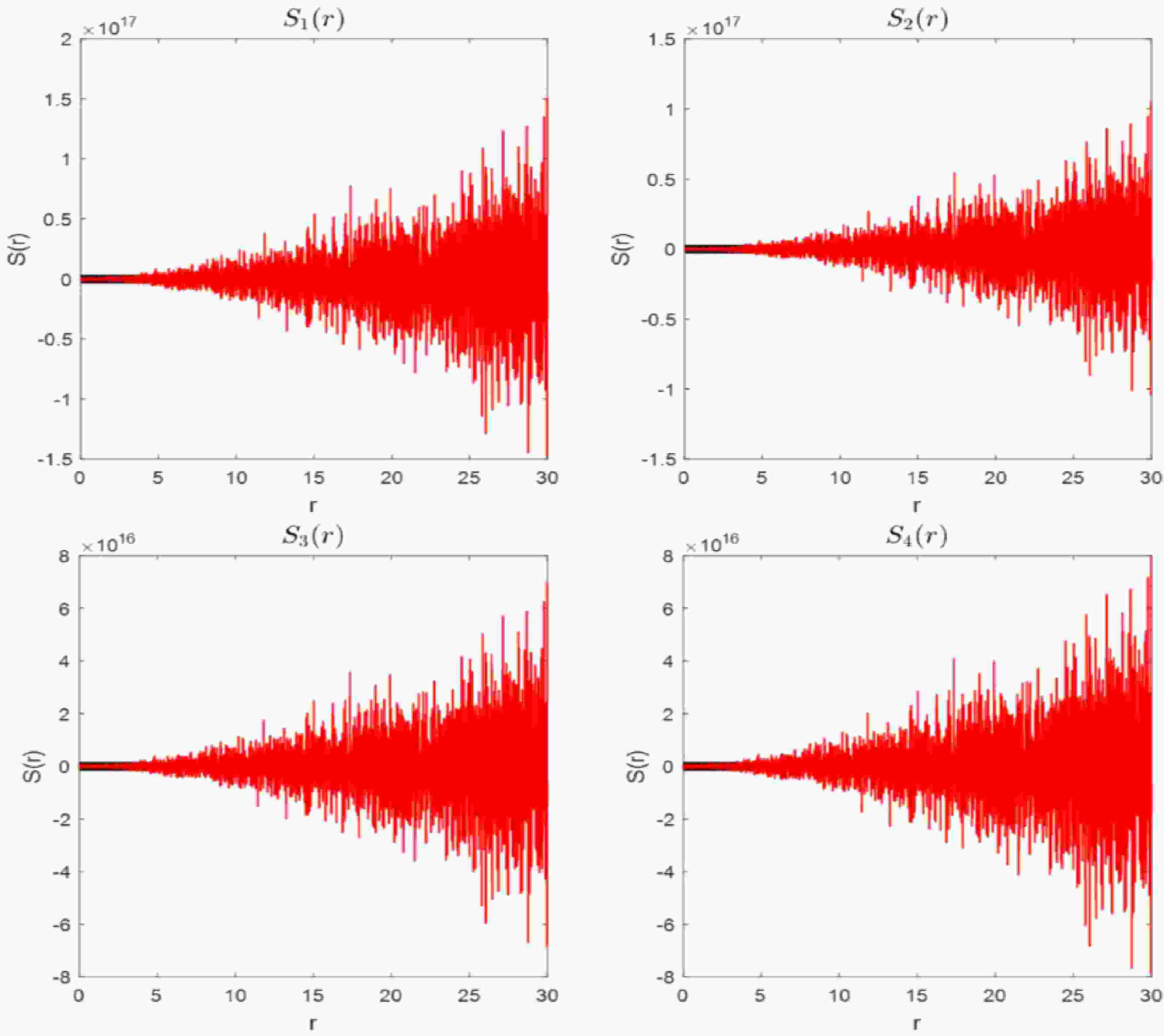
They span more than 15 orders of magnitude. The resulting condition number of K is therefore extremely large, confirming that the underlying inverse problem is severely ill-conditioned. As shown in Fig. 1, the unregularized reconstructions (red curve) exhibit pronounced, unphysical oscillations and deviate significantly from the benchmark (black curve). This oscillatory behavior provides direct numerical evidence of the ill-posedness of the inverse problem, indicating that even minor input perturbations can induce substantial instabilities in the solution. Critically, this instability is fundamental: it arises irrespective of whether the number of data points is larger, smaller, or equal to that of the source degrees of freedom, and it persists even with continuous input data [50, 51]. These results underscore the need to employ Tikhonov regularization to mitigate numerical artifacts.

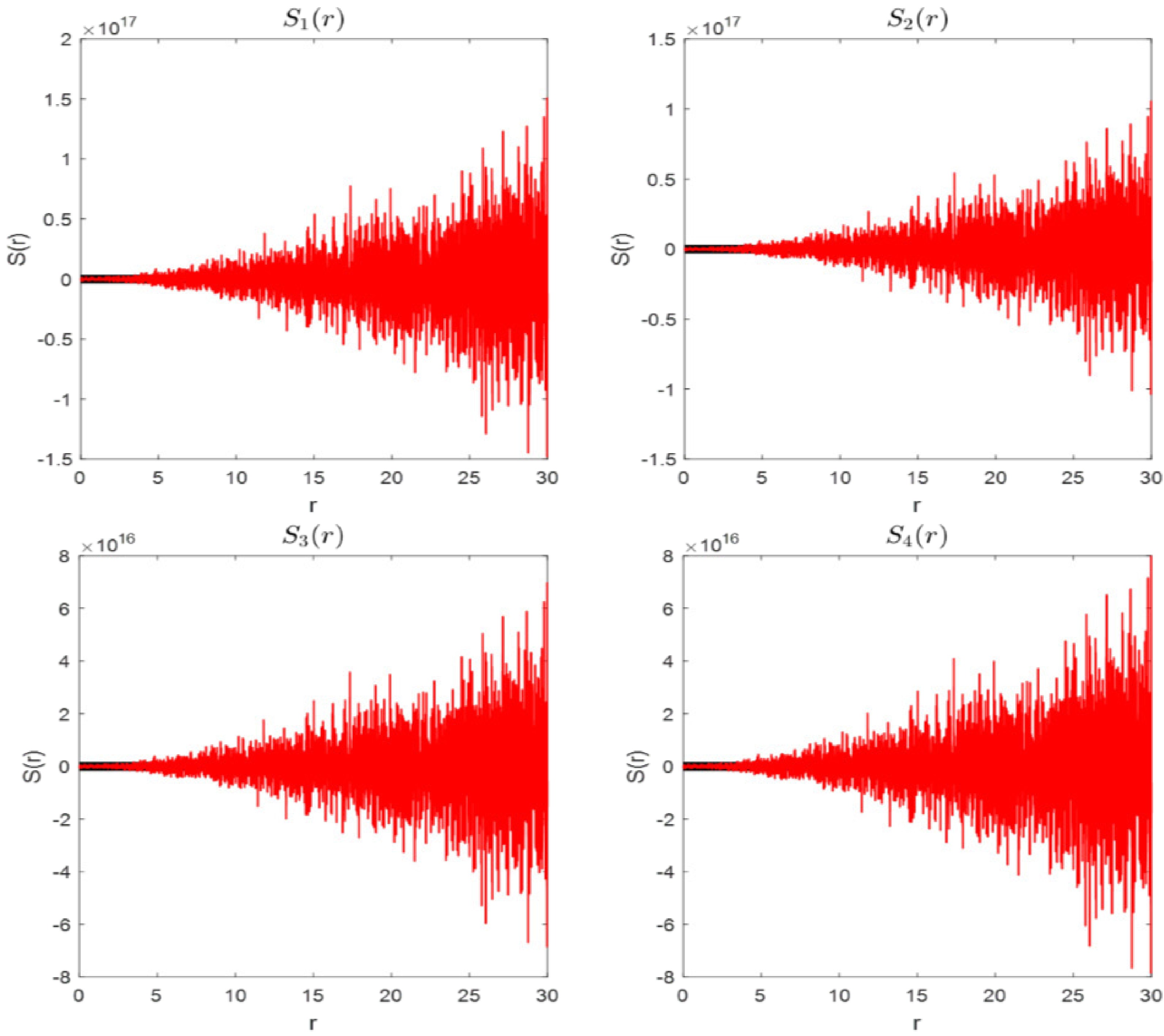
Figure 1.  (color online) The unregularized solutions (red curves) for the four sources exhibit unstable reconstructions that deviate from the benchmark solutions (black curves) by 17–18 orders of magnitude.

We now present reconstruction results using the Tikhonov regularization given by Eq. (12). The reconstructed source functions for the potential $ V_0=-10 {\rm{MeV}} $ are shown in Fig. 2 and Fig. 3, corresponding to 1% and 10% uncertainties, respectively. In each subfigure, the black curve denotes the benchmark source $ S_t $, the red curve represents the central reconstructed solution $ S_\alpha^\epsilon $, and the pink shaded region indicates the associated error band. This band quantifies the uncertainty estimated by generating multiple datasets through random sampling within the experimental error margins, inverting each independently, and computing one standard deviation around the mean of the resulting ensemble of source functions. With 1% uncertainty, the reconstructed solutions for both single- and mixed-Gaussian sources agree well with the benchmark. Notably, the retrieved $ S^\epsilon_\alpha $ naturally satisfies the normalization condition, with the integral approximately equal to unity. However, slight oscillations appear at large radii, as shown in Fig. 2. These oscillations are attributed to the rapid decay of the wave function in that region, which reduces the identifiability of the source. Although they lead to unphysical negative values in the reconstructed source, such artifacts are not a major concern here, as our primary focus is on the small-radius behavior, where the reconstruction is reliable. In future work, these issues could be further mitigated by incorporating additional prior information, such as non-negativity constraints.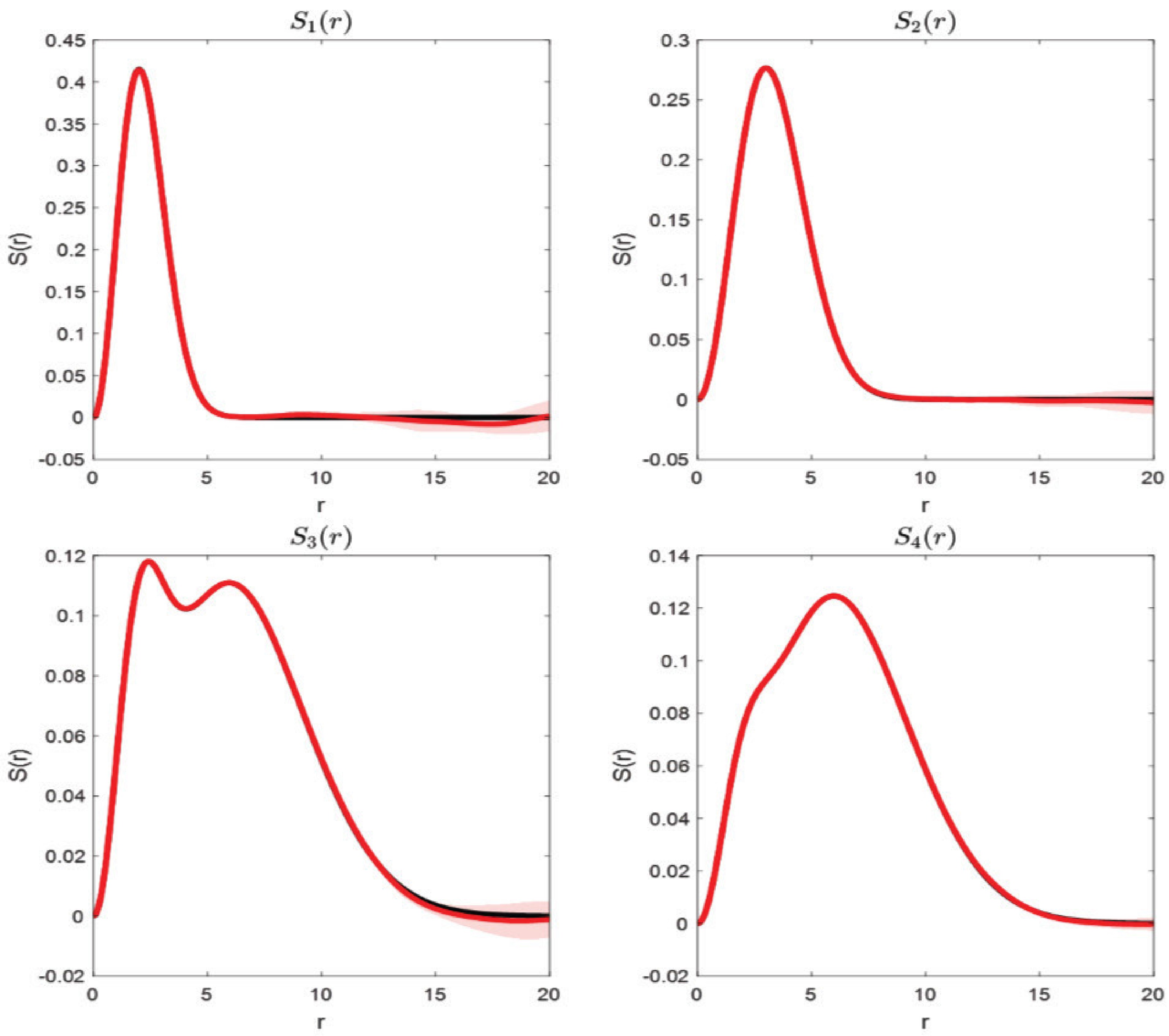

Figure 2.  (color online) The reconstructed solutions $ S_\alpha^\epsilon $ (red lines) and their associated error bands (pink shaded areas) for $ V_0=-10 {\rm{MeV}} $ with 1% uncertainty are compared to the benchmark $ S_t $ (black line).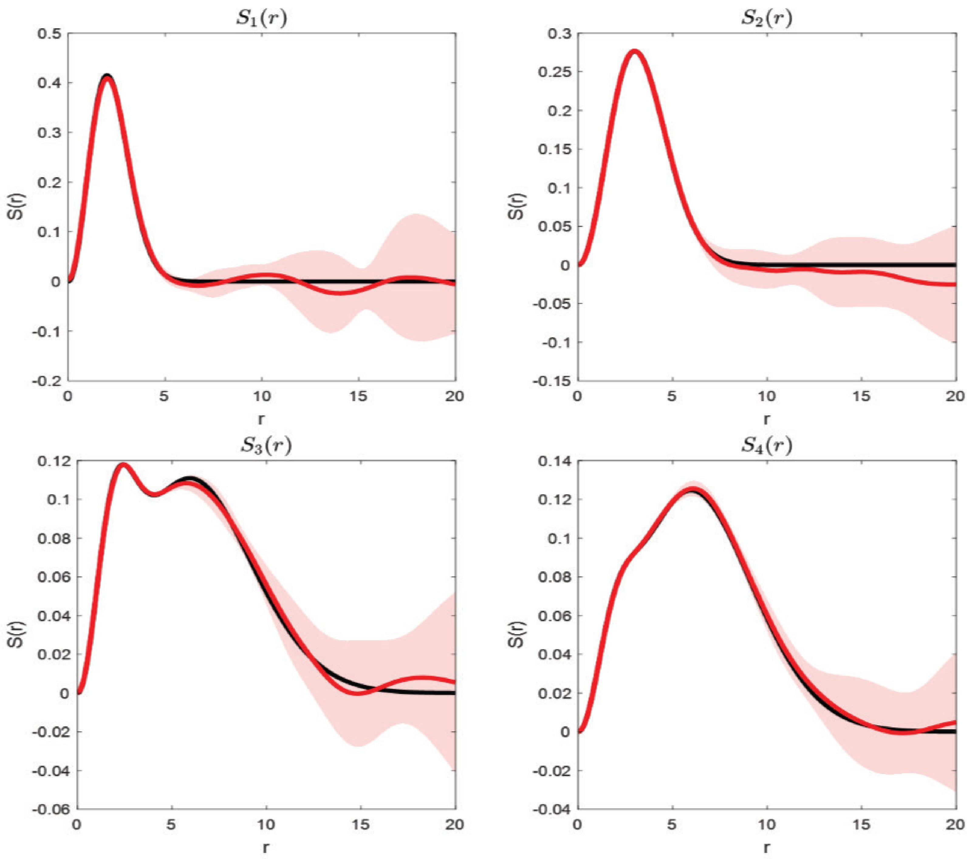

Figure 3.  (color online) Shown are the reconstructed solutions $ S_\alpha^\epsilon $ (red lines) and their associated error bands (pink shaded areas) for $ V_0=-10 {\rm{MeV}} $ with 10% uncertainty, compared with the benchmark $ S_t $ (black line).

In realistic experiments, CF uncertainties often exceed 1%. We therefore also consider the case with 10% uncertainty. As illustrated in Fig. 3, the reconstructed single-Gaussian source still matches the benchmark well near the peak, whereas some deviations occur for the mixed-Gaussian source. This suggests that sources with multiple peaks pose greater challenges for the method. Furthermore, the results indicate that reconstruction accuracy depends on the precision of the CFs. This behavior aligns with the theoretical foundation of Tikhonov regularization, as expressed in Eq. (14): as the input error decreases, the regularized solution converges to the true solution. To further validate our approach, we compute CFs using the reconstructed sources and the corresponding wave functions. For a representative case ($ V_0=-10\; {\rm{MeV}} $), we compare these with the true input CFs. As shown in Fig. 4, the CFs obtained from the central values of the reconstructed sources, combined with the associated wave functions (black curves), closely match the true input CFs (red curves). This agreement confirms the stability and reliability of our inverse approach.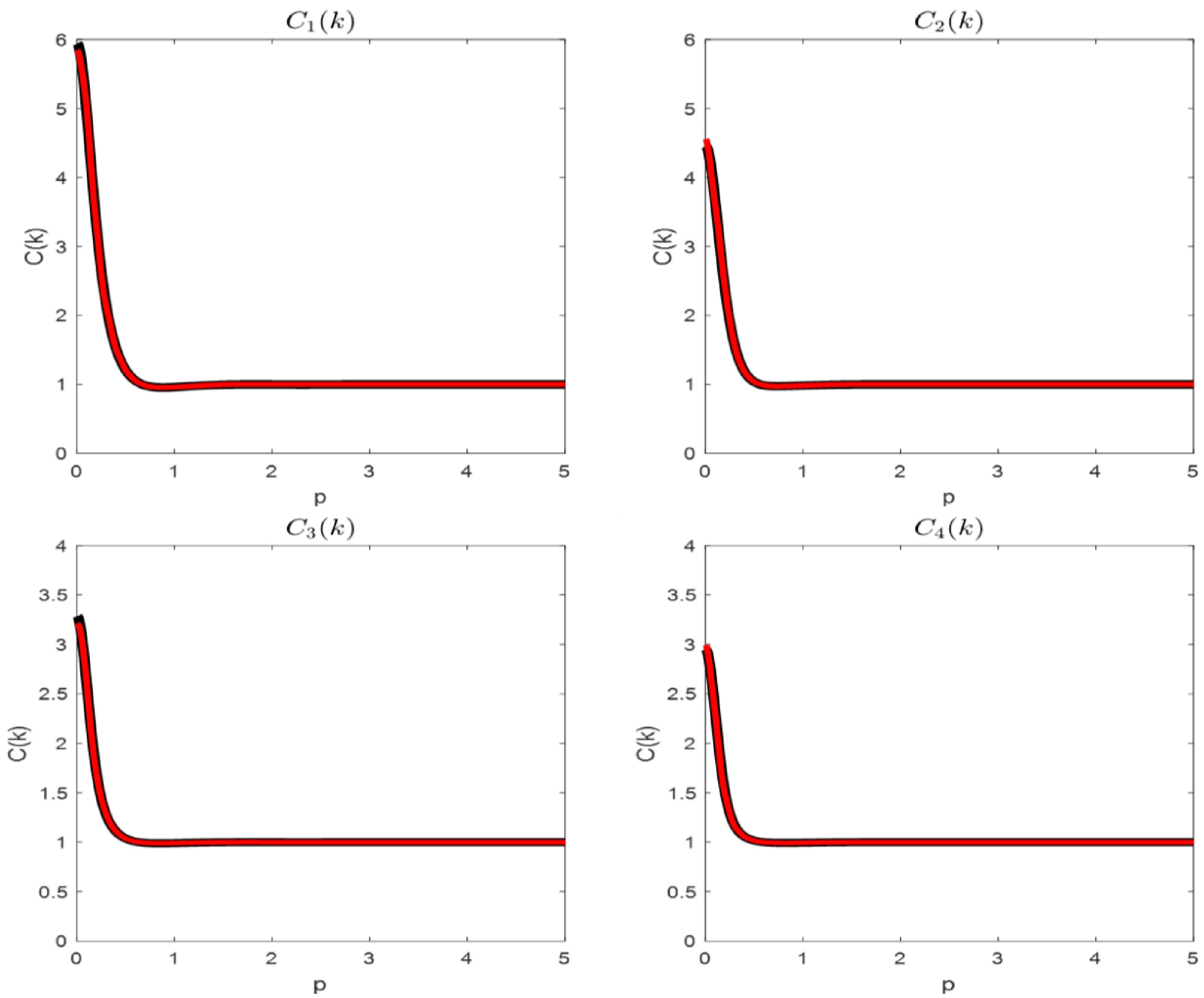

Figure 4.  (color online) Using the KP formula and taking $ V_0=-10 {\rm{MeV}} $ with a 10% uncertainty, we compare the correlation function computed from the central value of the reconstructed source, $ S_\alpha^\epsilon $, via the wave-function integral (red curve), with that derived from the benchmark source, $ S_t $ (black curve).

To investigate the general behavior under varying potential strengths, we reconstruct the source $ S_3(r,R) $ for three potentials: $ 25 $, $ -25 $, and $ -75 $ MeV. As shown in Fig. 3, the behavior of the mixed source $ S_3 $ is more complex than that of the other sources, making it a particularly stringent test for Tikhonov regularization. In Fig. 5, the reconstruction results under 10% and 1% uncertainties are presented in the top and bottom panels, respectively. In all scenarios, the reconstructed sources (red curves) align closely with the benchmark solutions (black curves). These findings affirm the effectiveness and versatility of the Tikhonov regularization approach in reconstructing different source functions across a range of interaction potentials. In short, the method achieves consistent accuracy whether the true source is a single Gaussian or a mixture of Gaussians, demonstrating reliable reconstruction of source functions with complex structures.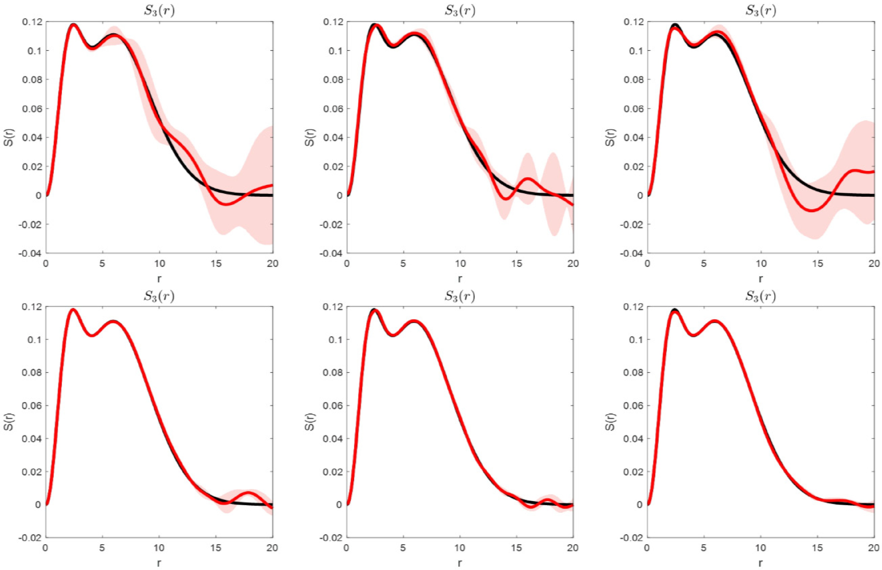

Figure 5.  (color online) Reconstruction of the source $ S_3 $ is shown under three potentials, 25,-25 and -75 MeV, with uncertainties of 10% (top row) and 1% (bottom row). The reconstructed solutions $ S_\alpha^\epsilon $ (red lines) and their associated error bands (pink shaded areas) are compared with the benchmark $ S_t $ (black line).

Momentum CFs are a well-established observable for probing hadron–hadron interactions. Conventional approaches often assume a Gaussian parameterization of the source function to infer these interactions from CFs, yet the exact form of the source function is not known a priori. Reconstructing the source function from known momentum CFs is an inverse problem. In this study, we introduce a mathematically rigorous approach to solve this inverse problem. In our calculations, we employ square-well potentials with four different strengths (repulsive, weakly attractive, moderately attractive, and deeply attractive) to derive analytic wave functions by solving the Schrödinger equation. Using these wave functions together with Gaussian and mixed-Gaussian source functions, we generate the corresponding momentum CFs. We then reconstruct the source functions from the momentum CFs using Tikhonov regularization.

Our results show that the source functions for all four scenarios are accurately reproduced. Both single- and mixed-Gaussian source functions are well recovered. We resampled the momentum CFs by introducing errors of 1% and 10%, revealing that the accuracy of the reconstructed source functions depends on the precision of the input CFs; as the uncertainties in the CFs increase, the fidelity of the reconstructed source functions degrades. Our results confirm that source functions can be reliably reconstructed using Tikhonov regularization when both wave functions and momentum CFs are known. This approach paves the way for extracting realistic source functions for various hadron pairs (meson–meson, meson–baryon, and baryon–baryon) as precise hadron–hadron interactions and experimental momentum CFs become available. Such source functions will be crucial for uncovering underlying physical properties and will, in turn, substantially improve the accuracy of hadron–hadron interactions extracted from momentum CFs.