


 Abstract
 HTML
HTML Reference
 Related
 PDF
PDF


-
Since the LHCb Collaboration found the strange-charm four-quark state candidate
$ X_{0,(1)}(2900) $ and$ T_{c\bar{s}}^{0(++)}(2900) $ [1−4], the open-charmed four-quark states have attracted increasing attention [5−19]. Subsequently, the doubly charmed four-quark state candidate$ T_{cc}^{+}(3875) $ , with the mass near$ (D^{+}D^0) $ threshold, [20–21] was reported in 2021. In the case of the fully charmed four-quark states, LHCb observed the broad candidate structure that ranged from 6.2 to 6.8 GeV and a narrow one located around 6.9 GeV in the$ J/\psi J/\psi $ channel [22]. These discoveries suggest that the heaviest open-charm four-quark state with triply charmed flavor should be possible. Although there is not yet sufficient experimental evidence for the existence, it has been many preliminary theoretical research to explore the properties of the exotic state at present [23−31]. In particular, regarding the mass spectrum of triply charmed four-quark states, Ref. [28] employed a quark-based model in conjunction with the Gaussian Expansion Method (GEM) and the Complex Scaling Method (CSM) to identify a triply heavy tetraquark state within the energy range of 5.6−5.9 GeV. In Ref.[26], the authors estimate the mass of the$ cc\bar{c}\bar{q} $ tetraquark state with quantum numbers$ J^{P} = 1^{+} $ to be$ 5.1\pm0.2 $ GeV using the operator product expansion (OPE). Furthermore, regarding the internal structure of states containing three heavy quarks, analogous to fully charmed four-quark states, conventional analyses disfavor a molecular configuration because the exchange of a single long-range light meson between two charmonium is suppressed. However, using heavy meson exchange forces [32, 33] or two light mesons exchange force [34], the authors considered the possibility of fully heavy four-quark molecular states. If such interactions do play an important role, the triply charmed four-quark molecular states should also be possible. Nevertheless, whether a stable or resonant triple charm four-quark state exists, and if so, whether its properties manifest as those of a compact tetraquark or an extended hadronic molecule, remains an open and fundamental question in hadron physics. Regardless of the ongoing theoretical debate, there is strong motivation for a systematic investigation of its potential phenomenological signatures, which can yield concrete theoretical predictions to provide direct guidance for experimental searches.We focus on the production and decay properties of the molecular states
$ cc\bar c\bar q $ in the phenomenological analysis and effective Lagrangian approach. The SU(3) flavor symmetry analysis [35−42] and the effective Lagrangian approach [43−47], which have been successfully applied to heavy meson and baryon systems, can accordingly be used to investigate the molecular states$ cc\bar c\bar q $ . With the assumption of molecular state, then the discussion of dynamics is possible. The hypothesis of hadronic molecule is popular, such as the four-quark candidate ψ(4040) is considered as$ D^{*} $ $ D^{*} $ hadronic molecule [48, 49]. The$ Y(4220) $ ,$ Z_c(3900) $ , and$ X(3872) $ states are interpreted as$ {\bar D}_1 D $ ,$ {\bar D}^* D $ , and$ {\bar D}^* D $ molecular states respectively [50, 51]. Moreover, the open-charm four-quark candidate$ T_{cc}^{+}(3875) $ is discussed under the molecular state$ (D^{+}D^{*0}) $ [21, 19]. Accordingly, in this work we adopt the generic schemes for the triply charmed molecule with$ J^P = 1^+ $ , pseudoscalar-vector$ \eta_c D^{*} $ ($ PV $ ) and vector-vector$ {J/\psi D^{*}} $ ($ VV $ ) configurations. The work proceeds following the standard procedure of the effective Lagrangian approach. We firstly establish a gauge invariant phenomenological Lagrangian to describe the interactions between molecular states and their components, whose associated coupling constants can be determined by the bare compositeness condition. A direct calculation depending on the Lagrangian at the hadronic level can then be carried out. To facilitate the calculation, we primarily consider the leading order triangle diagram contribution to the strong decay process involving$ c\bar c $ annihilation in$ J/\psi D^* $ or$ \eta_c D^* $ systems, as this process is suppressed by the OZI rule and the heavy charm quark mass.This paper is organized as follows. In Sec. II, we concisely analyze the properties of the molecular states
$ {{\eta}_cD^*} $ and$ {J/\psi D^*} $ , including their production and decay processes. The numerical results and corresponding discussions are presented in Sec. III. A summary of the work is provided in the final section. -
Since the LHCb Collaboration found the strange-charm four-quark state candidate
$ X_{0,(1)}(2900) $ and$ T_{c\bar{s}}^{0(++)}(2900) $ [1−4], the open-charmed four-quark states have attracted increasing attention [5−11, 13−19, 52]. Subsequently, the doubly charmed four-quark state candidate$ T_{cc}^{+}(3875) $ , with the mass near$ (D^{+}D^0) $ threshold, [20, 21] was reported in 2021. In the case of the fully charmed four-quark states, LHCb observed the broad candidate structure that ranged from 6.2 to 6.8 GeV and a narrow one located around 6.9 GeV in the$ J/\Psi J/\Psi $ channel [22]. These discoveries suggest that the heaviest open-charm four-quark state with triply charmed flavor should be possible. Although there is not yet sufficient experimental evidence for the existence, it has been many preliminary theoretical research to explore the properties of the exotic state at present [24−32]. In particular, regarding the mass spectrum of triply charmed four-quark states, Ref. [29] employed a quark-based model in conjunction with the Gaussian Expansion Method (GEM) and the Complex Scaling Method (CSM) to identify a triply heavy tetraquark state within the energy range of 5.6-5.9 GeV. In Ref.[27], the authors estimate the mass of the$ cc\bar{c}\bar{q} $ tetraquark state with quantum numbers$ J^{P} = 1^{+} $ to be$ 5.1\pm0.2 $ GeV using the operator product expansion (OPE). Furthermore, regarding the internal structure of states containing three heavy quarks, analogous to fully charmed four-quark states, conventional analyses disfavor a molecular configuration because the exchange of a single long-range light meson between two charmonium is suppressed. However, using heavy meson exchange forces [36, 37] or two light mesons exchange force [38], the authors considered the possibility of fully heavy four-quark molecular states. If such interactions do play an important role, the triply charmed four-quark molecular states should also be possible. Nevertheless, whether a stable or resonant triple charm four-quark state exists, and if so, whether its properties manifest as those of a compact tetraquark or an extended hadronic molecule, remains an open and fundamental question in hadron physics. Regardless of the ongoing theoretical debate, there is strong motivation for a systematic investigation of its potential phenomenological signatures, which can yield concrete theoretical predictions to provide direct guidance for experimental searches.We focus on the production and decay properties of the molecular states
$ cc\bar c\bar q $ in the phenomenological analysis and effective Lagrangian approach. The SU(3) flavor symmetry analysis [39−46] and the effective Lagrangian approach [47−51], which have been successfully applied to heavy meson and baryon systems, can accordingly be used to investigate the molecular states$ cc\bar c\bar q $ . With the assumption of molecular state, then the discussion of dynamics is possible. The hypothesis of hadronic molecule is popular, such as the four-quark candidate ψ(4040) is considered as$ D^{*} $ $ D^{*} $ hadronic molecule [33, 34]. The$ Y(4220) $ ,$ Z_c(3900) $ , and$ X(3872) $ states are interpreted as$ {\bar D}_1 D $ ,$ {\bar D}^* D $ , and$ {\bar D}^* D $ molecular states respectively [23, 35]. Moreover, the open-charm four-quark candidate$ T_{cc}^{+}(3875) $ is discussed under the molecular state$ (D^{+}D^{*0}) $ [21, 52]. Accordingly, in this work we adopt the generic schemes for the triply charmed molecule with$ J^P = 1^+ $ , pseudoscalar-vector$ \eta_c D^{*} $ ($ PV $ ) and vector-vector$ {J/\psi D^{*}} $ ($ VV $ ) configurations. The work proceeds following the standard procedure of the effective Lagrangian approach. We firstly establish a gauge invariant phenomenological Lagrangian to describe the interactions between molecular states and their components, whose associated coupling constants can be determined by the bare compositeness condition. A direct calculation depending on the Lagrangian at the hadronic level can then be carried out. To facilitate the calculation, we primarily consider the leading order triangle diagram contribution to the strong decay process involving$ c\bar c $ annihilation in$ J/\Psi D^* $ or$ \eta_c D^* $ systems, as this process is suppressed by the OZI rule and the heavy charm quark mass.This paper is organized as follows. In Sec. II, we concisely analyze the properties of the molecular states
$ {{\eta}_cD^*} $ and$ {J/\psi D^*} $ , including their production and decay processes. The numerical results and corresponding discussions are presented in Sec. III. A summary of the work is provided in the final section. -
Since the LHCb Collaboration found the strange-charm four-quark state candidate
$ X_{0,(1)}(2900) $ and$ T_{c\bar{s}}^{0(++)}(2900) $ [1−4], the open-charmed four-quark states have attracted increasing attention [5−19]. Subsequently, the doubly charmed four-quark state candidate$ T_{cc}^{+}(3875) $ , with the mass near$ (D^{+}D^0) $ threshold, [20–21] was reported in 2021. In the case of the fully charmed four-quark states, LHCb observed the broad candidate structure that ranged from 6.2 to 6.8 GeV and a narrow one located around 6.9 GeV in the$ J/\psi J/\psi $ channel [22]. These discoveries suggest that the heaviest open-charm four-quark state with triply charmed flavor should be possible. Although there is not yet sufficient experimental evidence for the existence, it has been many preliminary theoretical research to explore the properties of the exotic state at present [23−31]. In particular, regarding the mass spectrum of triply charmed four-quark states, Ref. [28] employed a quark-based model in conjunction with the Gaussian Expansion Method (GEM) and the Complex Scaling Method (CSM) to identify a triply heavy tetraquark state within the energy range of 5.6−5.9 GeV. In Ref.[26], the authors estimate the mass of the$ cc\bar{c}\bar{q} $ tetraquark state with quantum numbers$ J^{P} = 1^{+} $ to be$ 5.1\pm0.2 $ GeV using the operator product expansion (OPE). Furthermore, regarding the internal structure of states containing three heavy quarks, analogous to fully charmed four-quark states, conventional analyses disfavor a molecular configuration because the exchange of a single long-range light meson between two charmonium is suppressed. However, using heavy meson exchange forces [32, 33] or two light mesons exchange force [34], the authors considered the possibility of fully heavy four-quark molecular states. If such interactions do play an important role, the triply charmed four-quark molecular states should also be possible. Nevertheless, whether a stable or resonant triple charm four-quark state exists, and if so, whether its properties manifest as those of a compact tetraquark or an extended hadronic molecule, remains an open and fundamental question in hadron physics. Regardless of the ongoing theoretical debate, there is strong motivation for a systematic investigation of its potential phenomenological signatures, which can yield concrete theoretical predictions to provide direct guidance for experimental searches.We focus on the production and decay properties of the molecular states
$ cc\bar c\bar q $ in the phenomenological analysis and effective Lagrangian approach. The SU(3) flavor symmetry analysis [35−42] and the effective Lagrangian approach [43−47], which have been successfully applied to heavy meson and baryon systems, can accordingly be used to investigate the molecular states$ cc\bar c\bar q $ . With the assumption of molecular state, then the discussion of dynamics is possible. The hypothesis of hadronic molecule is popular, such as the four-quark candidate ψ(4040) is considered as$ D^{*} $ $ D^{*} $ hadronic molecule [48, 49]. The$ Y(4220) $ ,$ Z_c(3900) $ , and$ X(3872) $ states are interpreted as$ {\bar D}_1 D $ ,$ {\bar D}^* D $ , and$ {\bar D}^* D $ molecular states respectively [50, 51]. Moreover, the open-charm four-quark candidate$ T_{cc}^{+}(3875) $ is discussed under the molecular state$ (D^{+}D^{*0}) $ [21, 19]. Accordingly, in this work we adopt the generic schemes for the triply charmed molecule with$ J^P = 1^+ $ , pseudoscalar-vector$ \eta_c D^{*} $ ($ PV $ ) and vector-vector$ {J/\psi D^{*}} $ ($ VV $ ) configurations. The work proceeds following the standard procedure of the effective Lagrangian approach. We firstly establish a gauge invariant phenomenological Lagrangian to describe the interactions between molecular states and their components, whose associated coupling constants can be determined by the bare compositeness condition. A direct calculation depending on the Lagrangian at the hadronic level can then be carried out. To facilitate the calculation, we primarily consider the leading order triangle diagram contribution to the strong decay process involving$ c\bar c $ annihilation in$ J/\psi D^* $ or$ \eta_c D^* $ systems, as this process is suppressed by the OZI rule and the heavy charm quark mass.This paper is organized as follows. In Sec. II, we concisely analyze the properties of the molecular states
$ {{\eta}_cD^*} $ and$ {J/\psi D^*} $ , including their production and decay processes. The numerical results and corresponding discussions are presented in Sec. III. A summary of the work is provided in the final section. -
We focus on possible S-wave molecular configurations with
$ J^P = 1^+ $ of the four-quark state$ T_{cc\bar{c}\bar{q}} $ . The possible molecular states can be either vector-vector configurations,$ T_{J/\psi D^{*}} $ ($ VV $ ), or vector-pseudoscalar configurations,$ T_{\eta_c D^{*}} $ ($ PV $ ). The effective Lagrangian that describes the couplings between a molecular state and its constituents is given in Ref. [53].$ \begin{aligned}[b] {\cal L}_{T_{{ \eta_c D ^*}}} (x) =\;& g_{{ T_{{ \eta_c D^*}}}} \, T_{\eta_c D^*}^{\mu}(x) \int dy \, \Phi(y^2) \, \eta_c(x+{\omega}_1 y) \, D^*_{\mu}(x-{\omega}_2 y),\,\\ {\cal L}_{T_{{ {J/\psi D^*}}}}(x) =\;& ig_{{ T_{{ {J/\psi D^*}}}}} \, \varepsilon_{\mu \nu \alpha \beta} \partial^{\mu}T_{J/\psi D^*}^{\nu}(x)\\&\times \int dy \, \Phi(y^2) \, J/\psi^{\alpha}(x+{\omega}_1 y) \, {D^*}^{\beta}(x-{\omega}_2 y).\, \end{aligned} $
(1) Among these, the Fourier transform of the correlation function is defined as [44, 54]:
$ \Phi(y^2) \, = \, \int \frac{d^4p}{(2\pi)^4} \, e^{-ip y} \, {\widetilde{\Phi}}(-p^2) \;\; \text{with}\;\; \widetilde\Phi(p_E^2) \doteq \exp( - p_E^2/\Lambda_{T}^2). $
(2) The coupling constants can be further obtained through renormalization of the mass operator, as depicted by the self-energy diagram in Fig. 1A.
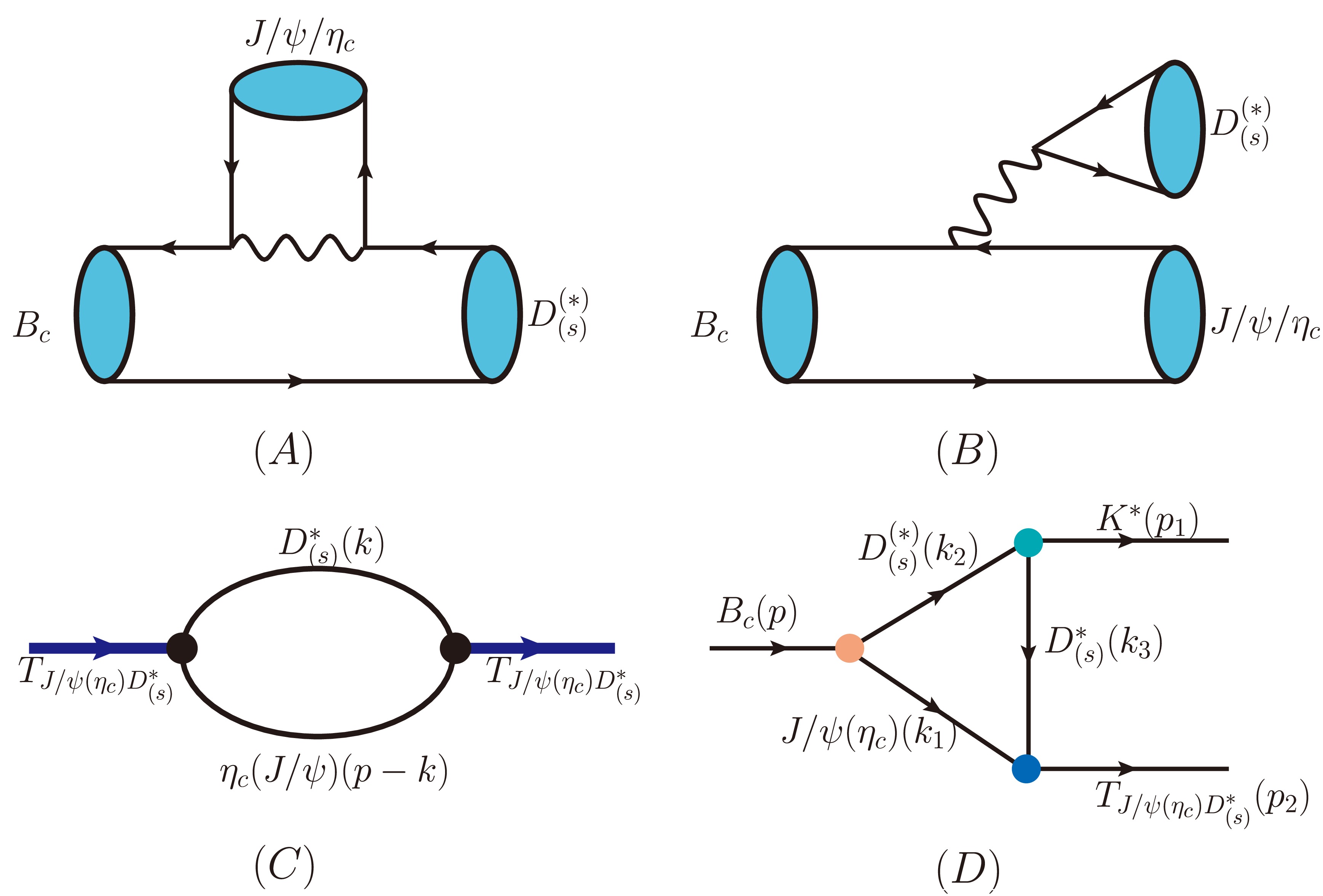
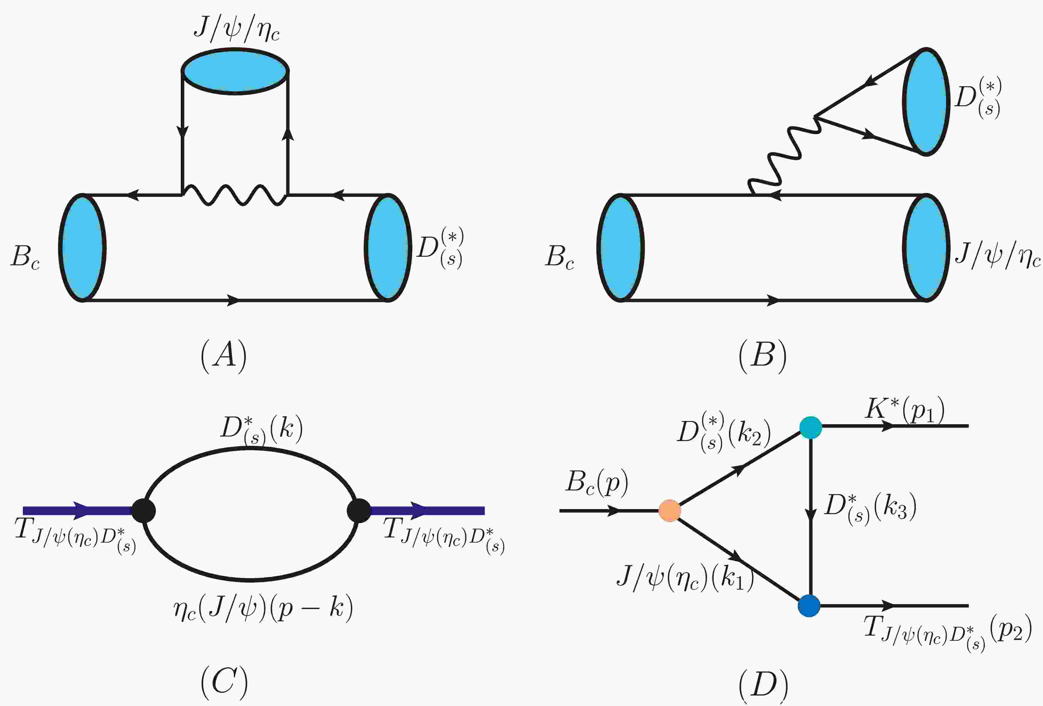
Figure 1. (color online) The internal W-emission (A) and external W-emission (B) diagrams represent the weak production of the molecular states
$ T_{\eta_c D^*} $ and$ T_{J/\psi D^*} $ in$ B_c $ meson decays. Diagrams (C) and (D) depict, respectively, the self-energy and production-triangle processes of the molecular states$ T_{J/\psi D^*} $ and$ T_{\eta_c D^*} $ .$ \begin{aligned}[b] \Sigma_{T}(p^2) =\;& \frac{g^2_{T_{{{{\eta_c D^*}}}}}}{3} \int \frac{{{\rm{d}}^{4}}k}{(2{\pi})^4i}\,\widetilde\Phi^2(-(k-pw)^2)\\&\frac{-3+\dfrac{k^2}{m^2_{D^*}}-\dfrac{(k\cdot p)^2}{m^2_{T_{\eta_c D^*}}}}{(k^2-m^2_{D^*})((p-k)^2-m^2_{\eta_c})},\\ \Sigma^{\prime}_{T}(p^2) =\;& \frac{g^2_{T_{{{J/\psi D^*}}}}}{3} \int \frac{{{\rm{d}}^{4}}k}{(2{\pi})^4i}\,\widetilde\Phi^2(-(k-pw)^2)\\&\frac{{{\cal{A}}}}{(k^2-m^2_{J/\psi })((p-k)^2-m^2_{ D^*})}, \end{aligned} $
(3) where
$ \begin{aligned}[b] {{\cal{A}}} =\;& \frac{(-2k \cdot p+k^2+p^2)(k \cdot p)^2}{{m^2_{J/\psi}}{m^2_{D^*}}}-\frac{2(k \cdot p)^2}{{m^2_{J/\psi}}} \\&-\frac{2(k \cdot p-k^2)(p^2-k \cdot p)(k \cdot p)}{{m^2_{J/\psi}}{m^2_{D^*}}}+\frac{k^2(p^2-k \cdot p)^2}{{m^2_{J/\psi}}{m^2_{D^*}}}\\&-6 p^2 + \frac{p^2(k \cdot p-k^2)^2}{{m^2_{J/\psi}}{m^2_{D^*}}} -\frac{k^2 p^2(k^2-2k \cdot p+p^2)}{{m^2_{J/\psi}}{m^2_{D^*}}}\\&+\frac{2 k^2 p^2}{{{m^2_{J/\psi}}}} - \frac{2(p^2-k \cdot p)^2}{{m^2_{D^*}}}+\frac{2 p^2(k^2-2k \cdot p+p^2)}{{m^2_{D^*}}}. \end{aligned} $
(4) We use the Weinberg compositeness condition [55].
$ Z_{T} = 1 - \frac{d\Sigma^{(\prime)}_{T}}{dp^2}\bigg|_{p^2 = m^2_{T}} = 0 \,. $
(5) We derive expressions for the coupling constants
$ g_{T_{\eta_c D^*}} $ and$ g_{T_{J/\psi D^*}} $ , and adopt$ \Lambda_T $ in the range 0.8 to 1.2 GeV in the numerical analysis. These expressions are provided in Appendix A. -
We focus on possible S-wave molecular configurations with
$ J^P = 1^+ $ of the four-quark state$ T_{cc\bar{c}\bar{q}} $ . The possible molecular states can be either vector-vector configurations,$ T_{J/\psi D^{*}} $ ($ VV $ ), or vector-pseudoscalar configurations,$ T_{\eta_c D^{*}} $ ($ PV $ ). The effective Lagrangian that describes the couplings between a molecular state and its constituents is given in Ref. [52].$ \begin{aligned}[b] {\cal L}_{T_{{ \eta_c D ^*}}} (x) =\;& g_{{ T_{{ \eta_c D^*}}}} \, T_{\eta_c D^*}^{\mu}(x) \int {\rm d}y \, \Phi(y^2) \, \eta_c(x+{\omega}_1 y) \, D^*_{\mu}(x-{\omega}_2 y),\,\\ {\cal L}_{T_{{ {J/\psi D^*}}}}(x) =\;& {\rm i} g_{{ T_{{ {J/\psi D^*}}}}} \, \varepsilon_{\mu \nu \alpha \beta} \partial^{\mu}T_{J/\psi D^*}^{\nu}(x)\\&\times \int {\rm d}y \, \Phi(y^2) \, J/\psi^{\alpha}(x+{\omega}_1 y) \, {D^*}^{\beta}(x-{\omega}_2 y).\, \end{aligned} $
(1) Among these, the Fourier transform of the correlation function is defined as [40, 53]:
$ \Phi(y^2) \, = \, \int \frac{{\rm d}^4p}{(2\pi)^4} \, {\rm e}^{-{\rm i}p y} \, {\widetilde{\Phi}}(-p^2) \;\; \text{with}\;\; \widetilde\Phi(p_E^2) \doteq \exp( - p_E^2/\Lambda_{T}^2). $
(2) The coupling constants can be further obtained through renormalization of the mass operator, as depicted by the self-energy diagram in Fig. 1(A).
Figure 1. (color online) The internal W-emission (A) and external W-emission (B) diagrams represent the weak production of the molecular states
$ T_{\eta_c D^*} $ and$ T_{J/\psi D^*} $ in$ B_c $ meson decays. Diagrams (C) and (D) depict, respectively, the self-energy and production-triangle processes of the molecular states$ T_{J/\psi D^*} $ and$ T_{\eta_c D^*} $ .$ \begin{aligned}[b] \Sigma_{T}(p^2) =\;& \frac{g^2_{T_{{{{\eta_c D^*}}}}}}{3} \int \frac{{{\rm{d}}^{4}}k}{(2{\pi})^4{\rm i}}\,\widetilde\Phi^2(-(k-pw)^2)\\& \times \frac{-3+\dfrac{k^2}{m^2_{D^*}}-\dfrac{(k\cdot p)^2}{m^2_{T_{\eta_c D^*}}}}{(k^2-m^2_{D^*})((p-k)^2-m^2_{\eta_c})},\\ \Sigma^{\prime}_{T}(p^2) =\;& \frac{g^2_{T_{{{J/\psi D^*}}}}}{3} \int \frac{{{\rm{d}}^{4}}k}{(2{\pi})^4{\rm i}}\,\widetilde\Phi^2(-(k-pw)^2)\\& \times \frac{{{\cal{A}}}}{(k^2-m^2_{J/\psi })((p-k)^2-m^2_{ D^*})}, \end{aligned} $
(3) where
$ \begin{aligned}[b] {{\cal{A}}} =\;& \frac{(-2k \cdot p+k^2+p^2)(k \cdot p)^2}{{m^2_{J/\psi}}{m^2_{D^*}}}-\frac{2(k \cdot p)^2}{{m^2_{J/\psi}}} \\&-\frac{2(k \cdot p-k^2)(p^2-k \cdot p)(k \cdot p)}{{m^2_{J/\psi}}{m^2_{D^*}}}+\frac{k^2(p^2-k \cdot p)^2}{{m^2_{J/\psi}}{m^2_{D^*}}}\\&-6 p^2 + \frac{p^2(k \cdot p-k^2)^2}{{m^2_{J/\psi}}{m^2_{D^*}}} -\frac{k^2 p^2(k^2-2k \cdot p+p^2)}{{m^2_{J/\psi}}{m^2_{D^*}}}\\&+\frac{2 k^2 p^2}{{{m^2_{J/\psi}}}} - \frac{2(p^2-k \cdot p)^2}{{m^2_{D^*}}}+\frac{2 p^2(k^2-2k \cdot p+p^2)}{{m^2_{D^*}}}. \end{aligned} $
(4) We use the Weinberg compositeness condition [54].
$ Z_{T} = 1 - \frac{{\rm d}\Sigma^{(\prime)}_{T}}{{\rm d}p^2}\bigg|_{p^2 = m^2_{T}} = 0 \,. $
(5) We derive expressions for the coupling constants
$ g_{T_{\eta_c D^*}} $ and$ g_{T_{J/\psi D^*}} $ , and adopt$ \Lambda_T $ in the range 0.8 to 1.2 GeV in the numerical analysis. These expressions are provided in Appendix A. -
In this section, we first employ a phenomenological analysis to investigate the production and decay of these molecular states. A convenient phenomenological tool is an SU(3) flavor-symmetric analysis. In flavor space, the light mesons can be grouped into an SU(3) octet, and the triple-charm molecular states form an SU(3) triplet, which can be represented as
$ T_{cc\bar c \bar q} = \left( T^{0}_{cc \bar c \bar u} , T^{+}_{cc \bar c \bar d} , T^{+}_{cc \bar c \bar s} \right) $ . Similarly, the charmed mesons form a triplet$ D = ( D^0 , D^+ , D_s^+) $ . Production from the$ B_c $ meson must proceed via the weak transitions$ \bar b\to c\bar c \bar s/\bar d $ . Within the framework of an SU(3) flavor-symmetric analysis, the effective Hamiltonian can be written as:$ {\cal{H}} = a_{1}{B}_{c}(H_{3})^{i}({T_{cc\bar c\bar q}})_{j}{V}^{j}_{i}, \ \text{with}\ (H_{3})^{2} = V_{cd}^{*}, (H_{3})^{3} = V_{cs}^{*}. $
(6) Here, V denotes the vector meson field, the coefficient
$ a_{1} $ parameterizes nonperturbative effects, and$ (H_3)^i $ represents the weak transition vertex. Expanding this Hamiltonian yields all possible production processes, which are listed in Table A1 in Appendix A. Taking into account the CKM matrix elements and the experimental detection efficiency, we select three golden channels:channel amplitude channel amplitude $ B_c^+\to \rho^0 T_{cc\bar c\bar d}^{+} $ $ \frac{-a_1 V^*_{\text{cd}}}{\sqrt{2}} $ $ B_c^+\to K^{*+} T_{cc\bar c\bar u}^{0} $ $ a_1 V^*_{\text{cs}} $ $ B_c^+\to \overline{K}^{*0} T_{cc\bar c\bar d}^{+} $ $ a_1 V^*_{\text{cs}} $ $ B_c^+\to \overline{K}^{*0} T_{cc\bar c\bar s}^{+} $ $ a_1 V^*_{\text{cd}} $ $ B_c^+\to \rho^+ T_{cc\bar c\bar u}^{0} $ $ a_1 V^*_{\text{cd}} $ $ B_c^+\to \phi T_{cc\bar c\bar s}^{+} $ $ a_1 V^*_{\text{cs}} $ Table A1. The production of the molecular states
$ T_{cc\bar c\bar q} $ from$ B_c $ mesons. The state$ T_{cc\bar c\bar q} $ can be realized as the molecules$ T_{\eta_c D^*} $ and$ T_{J/\psi D^*} $ .$ B_c^+\to {{\overline K}^{*0}} T_{cc\bar c\bar s}^+ , \,\,\, B_c^+\to {K^{*+}} T_{cc\bar c \bar u}^{0} , \,\,\, B_c^+\to {K^{*0}} T_{cc\bar c\bar d}^+ . $
(7) Neglecting phase-space effects leads to simplified relations among the different channels.
$ \frac{\Gamma(B_c^+\to K^{*+} T_{cc\bar c\bar u}^{0})}{\Gamma(B_c^+\to \overline{K}^{*0} T_{cc\bar c\bar s}^+)} = \frac{\Gamma(B_c^+\to K^{*0} T_{cc\bar c\bar d}^+)}{\Gamma(B_c^+\to \overline{K}^{*0} T_{cc\bar c\bar s}^+)} = \frac{|V_{cs}|^2}{|V_{cd}|^2}.\,\, $
(8) It should be noted that
$ T_{cc\bar c\bar q} $ can be the molecular states$ T_{J/\psi D^*} $ and$ T_{\eta_c D^*} $ in production processes. However, in the strong decays of the four-quark molecular state, the phenomenology of$ T_{cc\bar{c}\bar{q}} $ may differ significantly between the two molecular configurations due to phase-space effects. Therefore, we write the Hamiltonians for the two-body and three-body decays, respectively.$ \begin{aligned}[b] {\cal{H}} =\;& b_{1}({T}_{{{J/\psi D^*}}})_i D^{i}J/\psi+b_{2}({T}_{{{J/\psi D^*}}})_i{D^*}^{i}\eta_c\\& +c_{1}({T}_{{{J/\psi D^*}}})_i \eta_c {D}^{j}{P}^i_j+c_{2}({T}_{{{J/\psi D^*}}})_i J/\psi {D}^{j}{M}^i_j\\ & + b^{\prime}_1({T}_{{{\eta_c D^*}}})_i D^{i}J/\psi +c^{\prime}_{1}({T}_{\eta_c D^*})_i \eta_c {D}^{j}{P}^i_j, \end{aligned} $
(9) where P denotes a pseudoscalar meson. Accordingly, we derive all possible decay processes (summarized in Table A2) and the relations among different decay channels (listed in Table 1).
$ \Gamma(T^0_{\eta_c D^{*}}\to J / \psi D^0) $ $ = \Gamma(T^+_{\eta_c D^{*}}\to J / \psi D^{+}) $ $ \Gamma(T^+_{\eta_c D^*}\to D^0 \eta_c \pi^+) $ $ =2\Gamma(T^+_{\eta_c D^*}\to D^+ \eta_c \pi^0 ) $ $ =\Gamma(T^{+}_{\eta_c D_s^*}\to \eta_c D^{*+}_s) $ $ =2\Gamma(T^0_{\eta_c D^*}\to D^0 \eta_c \pi^0 ) $ $ \Gamma(T_{J / \psi D^*}^{0}\to J / \psi D^0) $ $ =\Gamma(T_{J / \psi D^*}^{+}\to J / \psi D^+) $ $ \Gamma(T^+_{J / \psi D^*}\to D^0 J / \psi \pi^+ ) $ $ =2\Gamma(T^0_{J / \psi D^*}\to D^0 J / \psi \pi^0 ) $ $ =\Gamma(T_{J / \psi D_s^*}^{+}\to J / \psi D^+_s) $ =2 $ \Gamma(T^+_{J / \psi D^*}\to D^+ J / \psi \pi^0 ) $ $ \Gamma(T_{J / \psi D^*}^{0}\to \eta_c D^{*0}) $ $ =\Gamma(T_{J / \psi D^*}^{+}\to \eta_c D^{*+}) $ $ \Gamma(T^0_{J / \psi D^*}\to D^+ \eta_c \pi^- ) $ $ =\Gamma(T^+_{J/\psi D^*}\to D^0 \eta_c \pi^+ ) $ $ =\Gamma(T_{J / \psi D_s^*}^{+}\to \eta_c D^{*+}_s) $ $ =2\Gamma(T^0_{J / \psi D^*}\to D^0 \eta_c \pi^0 ) $ $ =2\Gamma(T^+_{J / \psi D^*}\to D^+ \eta_c \pi^0 ) $ Table 1. Decay relations among different channels for the possible four-quark molecular states
$ T_{J/\psi D^*} $ and$ T_{\eta_c D^*} $ .channel amplitude channel amplitude channel amplitude $ T_{J/\psi D^*}^{0}\to J/\psi D^0 $ $ \frac{b_1}{3} $ $ T_{J/\psi D^*}^{+}\to J/\psi D^+ $ $ \frac{b_1}{3} $ $ T_{J/\psi D_s^*}^{+}\to J/\psi D^+_s $ $ \frac{b_1}{3} $ $ T_{J/\psi D^*}^{0}\to \eta_c D^{*0} $ $ \frac{b_2}{3} $ $ T_{J/\psi D^*}^{+}\to \eta_c D^{*+} $ $ \frac{b_2}{3} $ $ T_{J/\psi D_s^*}^{+}\to \eta_c D^{*+}_s $ $ \frac{b_2}{3} $ $ T_{\eta_c D^*}^{0}\to J/\psi D^0 $ $ \frac{b_1^{\prime}}{3} $ $ T_{\eta_c D^*}^{+}\to J/\psi D^+ $ $ \frac{b_1^{\prime}}{3} $ $ T_{\eta_c D_s^*}^{+}\to J/\psi D^+_s $ $ \frac{b_1^{\prime}}{3} $ $ T_{J/\psi D^*}^{0}\to D^0 J/\psi \pi^0 $ $ \frac{c_1}{\sqrt{2}} $ $ T_{J/\psi D^*}^{0}\to D^0 J/\psi \eta_q $ $ \frac{c_1}{\sqrt{6}} $ $ T_{J/\psi D^*}^{0}\to D^+ J/\psi \pi^- $ $ c_1 $ $ T_{J/\psi D^*}^{0}\to D^+_s J/\psi K^- $ $ c_1 $ $ T_{J/\psi D^*}^{+}\to D^0 J/\psi \pi^+ $ $ c_1 $ $ T_{J/\psi D^*}^{+}\to D^+ J/\psi \pi^0 $ $ -\frac{c_1}{\sqrt{2}} $ $ T_{J/\psi D^*}^{+}\to D^+ J/\psi \eta_q $ $ \frac{c_1}{\sqrt{6}} $ $ T_{J/\psi D^*}^{+}\to D^+_s J/\psi \overline K^0 $ $ c_1 $ $ T_{J/\psi D_s^*}^{+}\to D^0 J/\psi K^+ $ $ c_1 $ $ T_{J/\psi D_s^*}^{+}\to D^+ J/\psi K^0 $ $ c_1 $ $ T_{J/\psi D_s^*}^{+}\to D^+_s J/\psi \eta_q $ $ -\sqrt{\frac{2}{3}} c_1 $ $ T_{J/\psi D^*}^{0}\to D^0 \eta_c \pi^0 $ $ \frac{c_2}{\sqrt{2}} $ $ T_{J/\psi D^*}^{0}\to D^0 \eta_c \eta_q $ $ \frac{c_2}{\sqrt{6}} $ $ T_{J/\psi D^*}^{0}\to D^+ \eta_c \pi^- $ $ c_2 $ $ T_{J/\psi D^*}^{0}\to D^+_s \eta_c K^- $ $ c_2 $ $ T_{J/\psi D^*}^{+}\to D^0 \eta_c \pi^+ $ $ c_2 $ $ T_{J/\psi D^*}^{+}\to D^+ \eta_c \pi^0 $ $ -\frac{c_2}{\sqrt{2}} $ $ T_{J/\psi D^*}^{+}\to D^+ \eta_c \eta_q $ $ \frac{c_2}{\sqrt{6}} $ $ T_{J/\psi D^*}^{+}\to D^+_s \eta_c \overline K^0 $ $ c_2 $ $ T_{J/\psi D_s^*}^{+}\to D^0 \eta_c K^+ $ $ c_2 $ $ T_{J/\psi D_s^*}^{+}\to D^+ \eta_c K^0 $ $ c_2 $ $ T_{J/\psi D_s^*}^{+}\to D^+_s \eta_c \eta_q $ $ -\sqrt{\frac{2}{3}} c_2 $ $ T_{\eta_c D_s^*}^{0}\to D^0 \eta_c \eta_q $ $ \frac{c_1^{\prime}}{\sqrt{6}} $ $ T_{\eta_c D^*}^{0}\to D^+ \eta_c \pi^- $ $ c_1^{\prime} $ $ T_{\eta_c D^*}^{0}\to D^+_s \eta_c K^- $ $ c_1^{\prime} $ $ T_{\eta_c D^*}^{+}\to D^0 \eta_c \pi^+ $ $ c_1^{\prime} $ $ T_{\eta_c D^*}^{+}\to D^+ \eta_c \pi^0 $ $ -\frac{c_1^{\prime}}{\sqrt{2}} $ $ T_{\eta_c D^*}^{+}\to D^+ \eta_c \eta_q $ $ \frac{c_1^{\prime}}{\sqrt{6}} $ $ T_{\eta_c D^*}^{+}\to D^+_s \eta_c \overline K^0 $ $ c_1^{\prime} $ $ T_{\eta_c D_s^*}^{+}\to D^0 \eta_c K^+ $ $ c_1^{\prime} $ $ T_{\eta_c D_s^*}^{+}\to D^+ \eta_c K^0 $ $ c_1^{\prime} $ $ T_{\eta_c D_s^*}^{0}\to D^0 \eta_c \pi^0 $ $ \frac{c_1^{\prime}}{\sqrt{2}} $ $ T_{\eta_c D_s^*}^{+}\to D^+_s \eta_c \eta_q $ $ -\sqrt{\frac{2}{3}} c_1^{\prime} $ Table A2. Two- and three-body decay processes of
$ T_{J/\psi D^*} $ and$ T_{\eta_c D^*} $ . -
In this section, we first employ a phenomenological analysis to investigate the production and decay of these molecular states. A convenient phenomenological tool is an SU(3) flavor-symmetric analysis. In flavor space, the light mesons can be grouped into an SU(3) octet, and the triple-charm molecular states form an SU(3) triplet, which can be represented as
$ T_{cc\bar c \bar q} = \left( T^{0}_{cc \bar c \bar u} , T^{+}_{cc \bar c \bar d} , T^{+}_{cc \bar c \bar s} \right) $ . Similarly, the charmed mesons form a triplet$ D = ( D^0 , D^+ , D_s^+) $ . Production from the$ B_c $ meson must proceed via the weak transitions$ \bar b\to c\bar c \bar s/\bar d $ . Within the framework of an SU(3) flavor-symmetric analysis, the effective Hamiltonian can be written as:$ {\cal{H}} = a_{1}{B}_{c}(H_{3})^{i}({T_{cc\bar c\bar q}})_{j}{V}^{j}_{i}, \ \text{with}\ (H_{3})^{2} = V_{cd}^{*}, (H_{3})^{3} = V_{cs}^{*}. $
(6) Here, V denotes the vector meson field, the coefficient
$ a_{1} $ parameterizes nonperturbative effects, and$ (H_3)^i $ represents the weak transition vertex. Expanding this Hamiltonian yields all possible production processes, which are listed in Table A1 in Appendix A. Taking into account the CKM matrix elements and the experimental detection efficiency, we select three golden channels:channel amplitude channel amplitude $ B_c^+\to \rho^0 T_{cc\bar c\bar d}^{+} $ $ \frac{-a_1 V^*_{\text{cd}}}{\sqrt{2}} $ $ B_c^+\to K^{*+} T_{cc\bar c\bar u}^{0} $ $ a_1 V^*_{\text{cs}} $ $ B_c^+\to \overline{K}^{*0} T_{cc\bar c\bar d}^{+} $ $ a_1 V^*_{\text{cs}} $ $ B_c^+\to \overline{K}^{*0} T_{cc\bar c\bar s}^{+} $ $ a_1 V^*_{\text{cd}} $ $ B_c^+\to \rho^+ T_{cc\bar c\bar u}^{0} $ $ a_1 V^*_{\text{cd}} $ $ B_c^+\to \phi T_{cc\bar c\bar s}^{+} $ $ a_1 V^*_{\text{cs}} $ Table A1. The production of the molecular states
$ T_{cc\bar c\bar q} $ from$ B_c $ mesons. The state$ T_{cc\bar c\bar q} $ can be realized as the molecules$ T_{\eta_c D^*} $ and$ T_{J/\psi D^*} $ .$ B_c^+\to {{\overline K}^{*0}} T_{cc\bar c\bar s}^+ , \,\,\, B_c^+\to {K^{*+}} T_{cc\bar c \bar u}^{0} , \,\,\, B_c^+\to {K^{*0}} T_{cc\bar c\bar d}^+ . $
(7) Neglecting phase-space effects leads to simplified relations among the different channels.
$ \frac{\Gamma(B_c^+\to K^{*+} T_{cc\bar c\bar u}^{0})}{\Gamma(B_c^+\to \overline{K}^{*0} T_{cc\bar c\bar s}^+)} = \frac{\Gamma(B_c^+\to K^{*0} T_{cc\bar c\bar d}^+)}{\Gamma(B_c^+\to \overline{K}^{*0} T_{cc\bar c\bar s}^+)} = \frac{|V_{cs}|^2}{|V_{cd}|^2}.\,\, $
(8) It should be noted that
$ T_{cc\bar c\bar q} $ can be the molecular states$ T_{J/\psi D^*} $ and$ T_{\eta_c D^*} $ in production processes. However, in the strong decays of the four-quark molecular state, the phenomenology of$ T_{cc\bar{c}\bar{q}} $ may differ significantly between the two molecular configurations due to phase-space effects. Therefore, we write the Hamiltonians for the two-body and three-body decays, respectively.$ \begin{aligned}[b] {\cal{H}} =\;& b_{1}({T}_{{{J/\psi D^*}}})_i D^{i}J/\psi+b_{2}({T}_{{{J/\psi D^*}}})_i{D^*}^{i}\eta_c\\& +c_{1}({T}_{{{J/\psi D^*}}})_i \eta_c {D}^{j}{P}^i_j+c_{2}({T}_{{{J/\psi D^*}}})_i J/\psi {D}^{j}{M}^i_j\\ & + b^{\prime}_1({T}_{{{\eta_c D^*}}})_i D^{i}J/\psi +c^{\prime}_{1}({T}_{\eta_c D^*})_i \eta_c {D}^{j}{P}^i_j, \end{aligned} $
(9) where P denotes a pseudoscalar meson. Accordingly, we derive all possible decay processes (summarized in Table A2) and the relations among different decay channels (listed in Table 1).
$ \Gamma(T^0_{\eta_c D^{*}}\to J / \psi D^0) = \Gamma(T^+_{\eta_c D^{*}}\to J / \psi D^{+}) =\Gamma(T^{+}_{\eta_c D_s^*}\to \eta_c D^{*+}_s)$ $ \Gamma(T^+_{\eta_c D^*}\to D^0 \eta_c \pi^+) =2\Gamma(T^+_{\eta_c D^*}\to D^+ \eta_c \pi^0 ) =2\Gamma(T^0_{\eta_c D^*}\to D^0 \eta_c \pi^0 )$ $ \Gamma(T_{J / \psi D^*}^{0}\to J / \psi D^0) =\Gamma(T_{J / \psi D^*}^{+}\to J / \psi D^+)=\Gamma(T_{J / \psi D_s^*}^{+}\to J / \psi D^+_s)$ $ \Gamma(T^+_{J / \psi D^*}\to D^0 J / \psi \pi^+ )=2\Gamma(T^0_{J / \psi D^*}\to D^0 J / \psi \pi^0 ) =2\Gamma(T^+_{J / \psi D^*}\to D^+ J / \psi \pi^0 )$ $ \Gamma(T_{J / \psi D^*}^{0}\to \eta_c D^{*0}) =\Gamma(T_{J / \psi D^*}^{+}\to \eta_c D^{*+})=\Gamma(T_{J / \psi D_s^*}^{+}\to \eta_c D^{*+}_s) $ $\begin{aligned}[b] \Gamma(T_{J / \psi D^*}^{0}\to D^+ \eta _c\pi^-) =\;&\Gamma(T^+_{J/\psi D^*}\to D^0 \eta_c \pi^+ ) =2\Gamma(T^0_{J / \psi D^*}\to D^0 \eta_c \pi^0 )\\=\;&2\Gamma(T^+_{J / \psi D^*}\to D^+ \eta_c \pi^0 )\end{aligned}$ Table 1. Decay relations among different channels for the possible four-quark molecular states
$ T_{J/\psi D^*} $ and$ T_{\eta_c D^*} $ .channel amplitude channel amplitude channel amplitude $ T_{J/\psi D^*}^{0}\to J/\psi D^0 $ $ \frac{b_1}{3} $ $ T_{J/\psi D^*}^{+}\to J/\psi D^+ $ $ \frac{b_1}{3} $ $ T_{J/\psi D_s^*}^{+}\to J/\psi D^+_s $ $ \frac{b_1}{3} $ $ T_{J/\psi D^*}^{0}\to \eta_c D^{*0} $ $ \frac{b_2}{3} $ $ T_{J/\psi D^*}^{+}\to \eta_c D^{*+} $ $ \frac{b_2}{3} $ $ T_{J/\psi D_s^*}^{+}\to \eta_c D^{*+}_s $ $ \frac{b_2}{3} $ $ T_{\eta_c D^*}^{0}\to J/\psi D^0 $ $ \frac{b_1^{\prime}}{3} $ $ T_{\eta_c D^*}^{+}\to J/\psi D^+ $ $ \frac{b_1^{\prime}}{3} $ $ T_{\eta_c D_s^*}^{+}\to J/\psi D^+_s $ $ \frac{b_1^{\prime}}{3} $ $ T_{J/\psi D^*}^{0}\to D^0 J/\psi \pi^0 $ $ \frac{c_1}{\sqrt{2}} $ $ T_{J/\psi D^*}^{0}\to D^0 J/\psi \eta_q $ $ \frac{c_1}{\sqrt{6}} $ $ T_{J/\psi D^*}^{0}\to D^+ J/\psi \pi^- $ $ c_1 $ $ T_{J/\psi D^*}^{0}\to D^+_s J/\psi K^- $ $ c_1 $ $ T_{J/\psi D^*}^{+}\to D^0 J/\psi \pi^+ $ $ c_1 $ $ T_{J/\psi D^*}^{+}\to D^+ J/\psi \pi^0 $ $ -\frac{c_1}{\sqrt{2}} $ $ T_{J/\psi D^*}^{+}\to D^+ J/\psi \eta_q $ $ \frac{c_1}{\sqrt{6}} $ $ T_{J/\psi D^*}^{+}\to D^+_s J/\psi \overline K^0 $ $ c_1 $ $ T_{J/\psi D_s^*}^{+}\to D^0 J/\psi K^+ $ $ c_1 $ $ T_{J/\psi D_s^*}^{+}\to D^+ J/\psi K^0 $ $ c_1 $ $ T_{J/\psi D_s^*}^{+}\to D^+_s J/\psi \eta_q $ $ -\sqrt{\frac{2}{3}} c_1 $ $ T_{J/\psi D^*}^{0}\to D^0 \eta_c \pi^0 $ $ \frac{c_2}{\sqrt{2}} $ $ T_{J/\psi D^*}^{0}\to D^0 \eta_c \eta_q $ $ \frac{c_2}{\sqrt{6}} $ $ T_{J/\psi D^*}^{0}\to D^+ \eta_c \pi^- $ $ c_2 $ $ T_{J/\psi D^*}^{0}\to D^+_s \eta_c K^- $ $ c_2 $ $ T_{J/\psi D^*}^{+}\to D^0 \eta_c \pi^+ $ $ c_2 $ $ T_{J/\psi D^*}^{+}\to D^+ \eta_c \pi^0 $ $ -\frac{c_2}{\sqrt{2}} $ $ T_{J/\psi D^*}^{+}\to D^+ \eta_c \eta_q $ $ \frac{c_2}{\sqrt{6}} $ $ T_{J/\psi D^*}^{+}\to D^+_s \eta_c \overline K^0 $ $ c_2 $ $ T_{J/\psi D_s^*}^{+}\to D^0 \eta_c K^+ $ $ c_2 $ $ T_{J/\psi D_s^*}^{+}\to D^+ \eta_c K^0 $ $ c_2 $ $ T_{J/\psi D_s^*}^{+}\to D^+_s \eta_c \eta_q $ $ -\sqrt{\frac{2}{3}} c_2 $ $ T_{\eta_c D_s^*}^{0}\to D^0 \eta_c \eta_q $ $ \frac{c_1^{\prime}}{\sqrt{6}} $ $ T_{\eta_c D^*}^{0}\to D^+ \eta_c \pi^- $ $ c_1^{\prime} $ $ T_{\eta_c D^*}^{0}\to D^+_s \eta_c K^- $ $ c_1^{\prime} $ $ T_{\eta_c D^*}^{+}\to D^0 \eta_c \pi^+ $ $ c_1^{\prime} $ $ T_{\eta_c D^*}^{+}\to D^+ \eta_c \pi^0 $ $ -\frac{c_1^{\prime}}{\sqrt{2}} $ $ T_{\eta_c D^*}^{+}\to D^+ \eta_c \eta_q $ $ \frac{c_1^{\prime}}{\sqrt{6}} $ $ T_{\eta_c D^*}^{+}\to D^+_s \eta_c \overline K^0 $ $ c_1^{\prime} $ $ T_{\eta_c D_s^*}^{+}\to D^0 \eta_c K^+ $ $ c_1^{\prime} $ $ T_{\eta_c D_s^*}^{+}\to D^+ \eta_c K^0 $ $ c_1^{\prime} $ $ T_{\eta_c D_s^*}^{0}\to D^0 \eta_c \pi^0 $ $ \frac{c_1^{\prime}}{\sqrt{2}} $ $ T_{\eta_c D_s^*}^{+}\to D^+_s \eta_c \eta_q $ $ -\sqrt{\frac{2}{3}} c_1^{\prime} $ Table A2. Two- and three-body decay processes of
$ T_{J/\psi D^*} $ and$ T_{\eta_c D^*} $ . -
Building on the SU(3) flavor-symmetry analysis, we proceed to investigate the dynamics of the molecular states
$ T_{J/\psi D^*} $ and$ T_{\eta_c D^*} $ within the effective Lagrangian approach. The production processes for these molecular states are depicted by the triangle diagram shown in Fig. 1(D). The corresponding amplitude can be expressed as:$\begin{aligned}[b]& \langle K^*T_{J/\psi(/\eta_c) D^*}|{\cal{H}}_{eff}| B_c\rangle \\=\;& \sum\limits_{\lambda}\langle K^*T_{J/\psi(/\eta_c) D^*}|{\cal{H}}_{\lambda}|M_1M_2\rangle\langle M_1M_2|{\cal{H}}_{eff}| B_c\rangle, \end{aligned}$
(10) Here,
$ \langle M_1M_2|{\cal{H}}_{eff}| B_c\rangle $ is the short-distance weak-decay matrix element;$ M_1 M_2 $ denote the possible final states of the$ B_c $ weak decay, and$ H_{eff} $ denotes the corresponding weak-decay Hamiltonian. In this process, the W-emission diagrams shown in Fig. 1(A,B) dominate the weak decay. The matrix element$ \langle K^*T_{J/\psi(/\eta_c) D^*}|{\cal{H}}_{\lambda}|M_1M_2\rangle $ describes the long-distance strong-coupling process, and$ {\cal{H}}_{\lambda} $ denotes the corresponding effective strong-interaction Hamiltonian. We write the effective weak-decay Hamiltonian as follows:$\begin{aligned}[b] {\cal{H}}_{eff} =\;& \frac{G_F}{\sqrt{2}} V_{cb}^*V_{cq} (C_1(\mu) (\bar b_{\alpha} c_{\beta})_{V-A}(\bar c_{\beta}q_{\alpha})_{V-A}\\&+C_2(\mu) (\bar b_{\alpha} c_{\alpha})_{V-A}(\bar c_{\beta}q_{\beta})_{V-A})+h.c. \,,\end{aligned} $
(11) where
$ G_F $ and$ C_{1,2}(\mu) $ are the Fermi constant and Wilson coefficients, respectively. The weak decay amplitude can be factorized into the product of the Wilson coefficients, the nonperturbative form factor, and the decay constant.$ \begin{aligned}[b]&{\cal{M}}( B_c \to J/\psi D(D^*)) \\=\;& \frac{G_F}{\sqrt{2}} V_{cb}^* V_{cs} a_{1,2} \langle J/\psi|(\bar b c)_{V-A} | B_c\rangle \langle D(D^*)|(\bar cq)_{V-A} |0\rangle \,,\end{aligned} $
(12) $\begin{aligned}[b]& {\cal{M}}( B_c \to \eta_c D(D^*)) \\=\;& \frac{G_F}{\sqrt{2}} V_{cb}^* V_{cs} a_{1,2} \langle \eta_c|(\bar b c)_{V-A} | B_c\rangle \langle D(D^*)|(\bar cq)_{V-A} |0\rangle \,, \end{aligned}$
(13) Here,
$ a_{1} $ and$ a_{2} $ denote the effective Wilson coefficients, with$ a_{1} = C_{1} + C_{2}/N_{c} $ and$ a_{2} = C_{2} + C_{1}/N_{c} $ . The parameter$ N_{c} $ denotes the number of colors. The form factors are defined as follows [56]:$ \begin{aligned}[b]& \langle J / \psi(p_{ { J / \psi}})|(\bar b c)_{V-A} | B_c(p_{{ B_c}})\rangle \\=\;& \frac{2}{m_{B_c}+m_V}\varepsilon_{\mu\nu\rho\sigma}\varepsilon^{*\nu}p_{{ B_c}}^{\rho} p_{ { J / \psi}}^{\sigma} A_0(q^2)+i\varepsilon_{\mu}^*(m_{B_c}+m_V)A_1(q^2)\\ & -i\frac{\varepsilon^*\cdot q}{m_{B_c}+m_V}(p_{{ B_c}}+p_{{ J/\psi}})_{\mu} A_2(q^2)-i \frac{\varepsilon^*\cdot q}{ q^2} 2 m_V {q}_{\mu} A_3(q^2) \\& +i \frac{\varepsilon^*\cdot {q}}{{q^2}} 2m_V {k_2}_{\mu} A_4(q^2) \,,\end{aligned} $
(14) $ \begin{aligned}[b]& \langle \eta_c(p_{{ \eta_c}})|(\bar b c)_{V-A} | B_c(p_{{ B_c}})\rangle\\ =\;& (p_{{ B_c}}+p_{{ \eta_c}}-\frac{m_{B_c}^2-m_P^2}{q^2}q)_{\mu} F_1(k^2_2)\\&+\frac{m_{B_c}^2-m_{\eta_c}^2}{q^2}{q}_{\mu} F_0(q^2). \end{aligned} $
(15) Here,
$ \varepsilon_{\mu} $ denotes the polarization vector of the$ J/\psi $ , and the transition momentum is defined as$ q_{\mu}\equiv(p_{B_c}-p_{J/\psi})_{\mu} $ . The matrix elements between the$ D^{(*)} $ meson and the vacuum are defined as [57]$ \langle D|(\bar c q)_{V-A} |0\rangle = i f_{D} \, q_{\mu} \,, \qquad \langle D^*| (\bar cq)_{V-A}|0 \rangle = m f_{D^*} \varepsilon^*_{\mu} \,, $
(16) where
$ f_{D^{(*)}} $ is the decay constant of the$ D^{(*)} $ meson, and$ \varepsilon_{\mu} $ denotes the polarization vector of the$ D^* $ meson.To address the long-distance strong-coupling matrix element, we introduce the following strong-interaction effective Lagrangian [58]:
$ \begin{aligned}[b] {\cal{L}}_{V P_1 P_2} =\;& i g_{V P_1 P_2}^{} \left( V_{\mu} \partial^{\mu} P_1 P_2 - V_{\mu} \partial^{\mu} P_2 P_1\right),\\ {\cal{L}}_{V_1 V_2 P} =\;& -g_{V_1 V_2 P}^{} \ \varepsilon^{\mu \nu \alpha \beta} \left(\partial_{\mu} V_{1 \nu} \partial_{\alpha} V_{2 \beta}\right) P,\\ {\cal{L}}_{D^* D^* J/\psi} =\;& -i g_{D^* D^* J/\psi}^{} \Bigl\{ {D^*}^{\mu}\left(\partial_{\mu} {D^*}^{\nu} {J/\psi} _{\nu} - {D^*}^{\nu} \partial_{\mu} {J/\psi} _{\nu}\right) \\&+ \left(\partial_{\mu}{D_{ \nu}^*} {D^*}^{\nu} - {D_{ \nu}^*} \partial_{\mu}{D^*}^{\nu} \right){J/\psi}^{\mu} \\ &+ {D^*}^{\mu}\left({D^*}^{\nu} \partial_{\mu} {J/\psi}_{ \nu} - \partial_{\mu} {D_{ \nu}^*}{J/\psi}^{\nu}\right) \Bigr\}, \end{aligned} $
(17) where
$ V_i $ and$ P_i $ denote the vector and pseudoscalar mesons, respectively.Using the effective Lagrangian and form factors, the amplitudes for
$ B_{c}\to K^*T_{J/\psi(/\eta_c) D^*} $ shown in Fig. 1(D) are given below:$ {\cal{M}}_{{T_{J/\psi D^*}}} = g_{{ T_{J/\psi D^*}}}\int\frac{d^4k_3}{(2\pi)^4}{\cal{F}}_2(k_3^2)\Big(\frac{2}{m_{B_c}+m_{J/\psi}} \varepsilon_{\varphi \nu \rho \sigma} p^{\rho} k_1^\sigma A_0(k_2^2)+i g_{\nu \varphi} A_1(k_2^2) (m_{B_c}+m_{J/\psi})-\frac{i {k_2}_{\nu}}{m_{B_c}+m_{J/\psi}}(p+k_1)_{\varphi} A_2(k_2^2) $
$ \begin{aligned}[b]&-2 i m_{J / \psi} \frac{{k_2}_{\nu} {k_2}_{\varphi}}{k_2^2} A_3(k_2^2) +2 i \frac{{k_2}_{\nu} k_{2\varphi}}{k_2^2} m_{J / \psi} A_4(k_2^2)\Big)(-g^{\nu\beta_1}+\frac{k_1^{\nu}k_1^{\beta_1}}{m_{J/\psi}^2})(-g^{\alpha_1\beta}+\frac{k_3^{\alpha_1}k_3^{\beta}}{m_{D^*}})p_2^\mu \varepsilon^{*\nu_1}(p_2)\varepsilon^{* n}(p_1)\\ &\times \Big\{\frac{if_{D_s}g_{{ D_sD^*K^*}} k_3^{\alpha}k_2^{\varphi} \varepsilon_{mn\alpha \beta} p_1^m }{(k_1^2-m_{J/\psi}^2)(k_3^2-m_{D^*}^2)(k_2^2-m_{D_s}^2)}+\frac{m_{D_s^*}f_{D_s^*}g_{{D_s^*D^*K^*}}(-g^{\varphi m}+\frac{k_2^{\varphi}k_2^{m}}{m_{D^*_s}})}{(k_1^2-m_{J/\psi}^2)(k_2^2-m_{D_s^*}^2)(k_3^2-m_{D^*}^2)}\\ & \varepsilon_{\mu \nu_1 \alpha_1 \beta_1} (i {k_2}_{n} g_{a m}-i {k_2}_{a} g_{n m}-i {k_3}_{m} g_{n a}+i {k_2}_{n} g_{\beta m}-i {p_1}_{ \beta} g_{n m}+i {p_1}_{ m} g_{n \beta})\Big\},\\ {\cal{M}}_{{T_{\eta_c D^*}}} =\;& \int \frac{d^4k_{{ 3}}}{(2\pi)^4}\Big(\frac{m_{B_c}^2-m_{\eta_c}^2}{k_2^2} {k_2}_{\rho}F_0(k_2^2)+(p+k_1-\frac{m_{B_c}^2-m_{\eta_c}^2}{k_2^2} k_2)_{\rho}{F}_1(k_2^2)\Big)\varepsilon^*_{\mu}(p_2)\varepsilon^{*n}(p_1)\\& g_{{ T_{\eta_c D^*}}}{\cal{F}}_2(k_3^2)(-g^{\beta \mu}+\frac{{k^\beta_3}{k^\mu_3}}{m_{D^*}^2}) \Big\{\frac{-g_{{ D_sD^*K^* }}\varepsilon_{m n \alpha \beta}p^{m}_1 k_3^\alpha k_2^\rho i f_{D_s}}{(k_{{ 1}}^2-m_{{ \eta_c}}^2)\ (k_{{ 2}}^2-m_{{ D_s}}^2)\ (k_{{ 3}}^2-m_{{ D^*}}^2)}({k_2}_{\beta} g_{n m}- {k_2}_{n} g_{\beta m}\\ &- {k_2}_{n} g_{m \beta}+ {p_1}_{ \beta} g_{n m}- {p_1}_{ m} g_{n \beta})+\frac{i{m_{D_s^*}f_{D_s^*}g_{D_s^*D^*K^*}(-g^{\rho m}+\frac{k_2^{\rho}k_2^{m}}{m_{D^*_s}})}}{(k_{{ 1}}^2-m_{{ J/\psi}}^2)\ (k_{{ 2}}^2-m_{{ D^*_s}}^2)\ (k_{{ 3}}^2-m_{{ D^*}}^2)} \Big\}. \end{aligned} $
(18) In addition, to remove ultraviolet divergences in the amplitudes, we introduce the form factor
$ {\cal{F}}_2(k_3^2) $ [59].$ {\cal{F}}_2(k_3^2) = \Big(\frac{m_{D^*}^2-\Lambda_{D^*}^2}{k_3^2-\Lambda_{D^*}^2}\Big)^2, $
(19) where
$ m_{D^{{*}}} $ and$ k_3 $ denote the mass and momentum of the exchanged meson$ D^{{*}} $ in the triangle diagrams. The cutoff parameter$ \Lambda_{D^*} = m_{D^{{*}}}+\alpha_m $ (with$ \alpha_m = \alpha \Lambda_{QCD} \approx $ 0.4 GeV)[35] is used to suppress contributions from hadrons at short distances. -
Building on the SU(3) flavor-symmetry analysis, we proceed to investigate the dynamics of the molecular states
$ T_{J/\psi D^*} $ and$ T_{\eta_c D^*} $ within the effective Lagrangian approach. The production processes for these molecular states are depicted by the triangle diagram shown in Fig. 1(D). The corresponding amplitude can be expressed as:$\begin{aligned}[b]& \langle K^*T_{J/\psi(/\eta_c) D^*}|{\cal{H}}_{\rm eff}| B_c\rangle \\=\;& \sum\limits_{\lambda}\langle K^*T_{J/\psi(/\eta_c) D^*}|{\cal{H}}_{\lambda}|M_1M_2\rangle\langle M_1M_2|{\cal{H}}_{\rm eff}| B_c\rangle. \end{aligned}$
(10) Here,
$\langle M_1M_2|{\cal{H}}_{\rm eff}| B_c\rangle$ is the short-distance weak-decay matrix element;$ M_1 M_2 $ denote the possible final states of the$ B_c $ weak decay, and$H_{\rm eff}$ denotes the corresponding weak-decay Hamiltonian. In this process, the W-emission diagrams shown in Fig. 1(A,B) dominate the weak decay. The matrix element$ \langle K^*T_{J/\psi(/\eta_c) D^*}|{\cal{H}}_{\lambda}|M_1M_2\rangle $ describes the long-distance strong-coupling process, and$ {\cal{H}}_{\lambda} $ denotes the corresponding effective strong-interaction Hamiltonian. We write the effective weak-decay Hamiltonian as follows:$\begin{aligned}[b] {\cal{H}}_{\rm eff} =\;& \frac{G_F}{\sqrt{2}} V_{cb}^*V_{cq} (C_1(\mu) (\bar b_{\alpha} c_{\beta})_{V-A}(\bar c_{\beta}q_{\alpha})_{V-A}\\&+C_2(\mu) (\bar b_{\alpha} c_{\alpha})_{V-A}(\bar c_{\beta}q_{\beta})_{V-A})+{\rm h.c.} \,,\end{aligned} $
(11) where
$ G_F $ and$ C_{1,2}(\mu) $ are the Fermi constant and Wilson coefficients, respectively. The weak decay amplitude can be factorized into the product of the Wilson coefficients, the nonperturbative form factor, and the decay constant.$ \begin{aligned}[b]&{\cal{M}}( B_c \to J/\psi D(D^*)) \\=\;& \frac{G_F}{\sqrt{2}} V_{cb}^* V_{cs} a_{1,2} \langle J/\psi|(\bar b c)_{V-A} | B_c\rangle \langle D(D^*)|(\bar cq)_{V-A} |0\rangle \,,\end{aligned} $
(12) $\begin{aligned}[b]& {\cal{M}}( B_c \to \eta_c D(D^*)) \\=\;& \frac{G_F}{\sqrt{2}} V_{cb}^* V_{cs} a_{1,2} \langle \eta_c|(\bar b c)_{V-A} | B_c\rangle \langle D(D^*)|(\bar cq)_{V-A} |0\rangle \,, \end{aligned}$
(13) Here,
$ a_{1} $ and$ a_{2} $ denote the effective Wilson coefficients, with$ a_{1} = C_{1} + C_{2}/N_{c} $ and$ a_{2} = C_{2} + C_{1}/N_{c} $ . The parameter$ N_{c} $ denotes the number of colors. The form factors are defined as follows [55]:$ \begin{aligned}[b]& \langle J / \psi(p_{ { J / \psi}})|(\bar b c)_{V-A} | B_c(p_{{ B_c}})\rangle \\=\;& \frac{2}{m_{B_c}+m_V}\varepsilon_{\mu\nu\rho\sigma}\varepsilon^{*\nu}p_{{ B_c}}^{\rho} p_{ { J / \psi}}^{\sigma} A_0(q^2)+ {\rm i}\varepsilon_{\mu}^*(m_{B_c}+m_V)A_1(q^2)\\ & -{\rm i}\frac{\varepsilon^*\cdot q}{m_{B_c}+m_V}(p_{{ B_c}}+p_{{ J/\psi}})_{\mu} A_2(q^2)- {\rm i} \frac{\varepsilon^*\cdot q}{ q^2} 2 m_V {q}_{\mu} A_3(q^2) \\& + {\rm i} \frac{\varepsilon^*\cdot {q}}{{q^2}} 2m_V {k_2}_{\mu} A_4(q^2) \,,\end{aligned} $
(14) $ \begin{aligned}[b]& \langle \eta_c(p_{{ \eta_c}})|(\bar b c)_{V-A} | B_c(p_{{ B_c}})\rangle\\ =\;& (p_{{ B_c}}+p_{{ \eta_c}}-\frac{m_{B_c}^2-m_P^2}{q^2}q)_{\mu} F_1(k^2_2)\\&+\frac{m_{B_c}^2-m_{\eta_c}^2}{q^2}{q}_{\mu} F_0(q^2). \end{aligned} $
(15) Here,
$ \varepsilon_{\mu} $ denotes the polarization vector of the$ J/\psi $ , and the transition momentum is defined as$ q_{\mu}\equiv(p_{B_c}-p_{J/\psi})_{\mu} $ . The matrix elements between the$ D^{(*)} $ meson and the vacuum are defined as [56]$ \langle D|(\bar c q)_{V-A} |0\rangle = {\rm i} f_{D} \, q_{\mu} \,, \qquad \langle D^*| (\bar cq)_{V-A}|0 \rangle = m f_{D^*} \varepsilon^*_{\mu} \,, $
(16) where
$ f_{D^{(*)}} $ is the decay constant of the$ D^{(*)} $ meson, and$ \varepsilon_{\mu} $ denotes the polarization vector of the$ D^* $ meson.To address the long-distance strong-coupling matrix element, we introduce the following strong-interaction effective Lagrangian [57]:
$ \begin{aligned}[b] {\cal{L}}_{V P_1 P_2} =\;& {\rm i} g_{V P_1 P_2}^{} \left( V_{\mu} \partial^{\mu} P_1 P_2 - V_{\mu} \partial^{\mu} P_2 P_1\right),\\ {\cal{L}}_{V_1 V_2 P} =\;& -g_{V_1 V_2 P}^{} \ \varepsilon^{\mu \nu \alpha \beta} \left(\partial_{\mu} V_{1 \nu} \partial_{\alpha} V_{2 \beta}\right) P,\\ {\cal{L}}_{D^* D^* J/\psi} =\;& - {\rm i} g_{D^* D^* J/\psi}^{} \Bigl\{ {D^*}^{\mu}\left(\partial_{\mu} {D^*}^{\nu} {J/\psi} _{\nu} - {D^*}^{\nu} \partial_{\mu} {J/\psi} _{\nu}\right) \\&+ \left(\partial_{\mu}{D_{ \nu}^*} {D^*}^{\nu} - {D_{ \nu}^*} \partial_{\mu}{D^*}^{\nu} \right){J/\psi}^{\mu} \\ &+ {D^*}^{\mu}\left({D^*}^{\nu} \partial_{\mu} {J/\psi}_{ \nu} - \partial_{\mu} {D_{ \nu}^*}{J/\psi}^{\nu}\right) \Bigr\}, \end{aligned} $
(17) where
$ V_i $ and$ P_i $ denote the vector and pseudoscalar mesons, respectively.Using the effective Lagrangian and form factors, the amplitudes for
$ B_{c}\to K^*T_{J/\psi(/\eta_c) D^*} $ shown in Fig. 1(D) are given below:$ {\cal{M}}_{{T_{J/\psi D^*}}} = g_{{ T_{J/\psi D^*}}}\int\frac{{\rm d}^4k_3}{(2\pi)^4}{\cal{F}}_2(k_3^2)\bigg(\frac{2}{m_{B_c}+m_{J/\psi}} \varepsilon_{\varphi \nu \rho \sigma} p^{\rho} k_1^\sigma A_0(k_2^2)+ {\rm i} g_{\nu \varphi} A_1(k_2^2) (m_{B_c}+m_{J/\psi})-\frac{{\rm i} {k_2}_{\nu}}{m_{B_c}+m_{J/\psi}}(p+k_1)_{\varphi} A_2(k_2^2) $
$ \begin{aligned}[b]&-2 {\rm i} m_{J / \psi} \frac{{k_2}_{\nu} {k_2}_{\varphi}}{k_2^2} A_3(k_2^2) +2{\rm i} \frac{{k_2}_{\nu} k_{2\varphi}}{k_2^2} m_{J / \psi} A_4(k_2^2)\bigg) \bigg(-g^{\nu\beta_1}+\frac{k_1^{\nu}k_1^{\beta_1}}{m_{J/\psi}^2}\bigg)\bigg(-g^{\alpha_1\beta}+\frac{k_3^{\alpha_1}k_3^{\beta}}{m_{D^*}}\bigg)p_2^\mu \varepsilon^{*\nu_1}(p_2)\varepsilon^{* n}(p_1)\\ &\times \bigg\{\frac{{\rm i}f_{D_s}g_{{ D_sD^*K^*}} k_3^{\alpha}k_2^{\varphi} \varepsilon_{mn\alpha \beta} p_1^m }{(k_1^2-m_{J/\psi}^2)(k_3^2-m_{D^*}^2)(k_2^2-m_{D_s}^2)}+\frac{m_{D_s^*}f_{D_s^*}g_{{D_s^*D^*K^*}}(-g^{\varphi m}+\frac{k_2^{\varphi}k_2^{m}}{m_{D^*_s}})}{(k_1^2-m_{J/\psi}^2)(k_2^2-m_{D_s^*}^2)(k_3^2-m_{D^*}^2)}\\ & \times \varepsilon_{\mu \nu_1 \alpha_1 \beta_1} ({\rm i} {k_2}_{n} g_{a m}- {\rm i} {k_2}_{a} g_{n m}- {\rm i} {k_3}_{m} g_{n a}+ {\rm i} {k_2}_{n} g_{\beta m}- {\rm i} {p_1}_{ \beta} g_{n m}+ {\rm i} {p_1}_{ m} g_{n \beta})\bigg\},\\ {\cal{M}}_{{T_{\eta_c D^*}}} =\;& \int \frac{{\rm d}^4k_{{ 3}}}{(2\pi)^4}\bigg(\frac{m_{B_c}^2-m_{\eta_c}^2}{k_2^2} {k_2}_{\rho}F_0(k_2^2)+(p+k_1-\frac{m_{B_c}^2-m_{\eta_c}^2}{k_2^2} k_2)_{\rho}{F}_1(k_2^2)\bigg)\varepsilon^*_{\mu}(p_2)\varepsilon^{*n}(p_1)\\& \times g_{{ T_{\eta_c D^*}}}{\cal{F}}_2(k_3^2)(-g^{\beta \mu}+\frac{{k^\beta_3}{k^\mu_3}}{m_{D^*}^2}) \bigg\{\frac{-g_{{ D_sD^*K^* }}\varepsilon_{m n \alpha \beta}p^{m}_1 k_3^\alpha k_2^\rho {\rm i} f_{D_s}}{(k_{{ 1}}^2-m_{{ \eta_c}}^2)\ (k_{{ 2}}^2-m_{{ D_s}}^2)\ (k_{{ 3}}^2-m_{{ D^*}}^2)}({k_2}_{\beta} g_{n m}- {k_2}_{n} g_{\beta m}\\ &- {k_2}_{n} g_{m \beta}+ {p_1}_{ \beta} g_{n m}- {p_1}_{ m} g_{n \beta})+\frac{{\rm i}{m_{D_s^*}f_{D_s^*}g_{D_s^*D^*K^*}(-g^{\rho m}+\frac{k_2^{\rho}k_2^{m}}{m_{D^*_s}})}}{(k_{{ 1}}^2-m_{{ J/\psi}}^2)\ (k_{{ 2}}^2-m_{{ D^*_s}}^2)\ (k_{{ 3}}^2-m_{{ D^*}}^2)} \bigg\}. \end{aligned} $
(18) In addition, to remove ultraviolet divergences in the amplitudes, we introduce the form factor
$ {\cal{F}}_2(k_3^2) $ [58].$ {\cal{F}}_2(k_3^2) = \Big(\frac{m_{D^*}^2-\Lambda_{D^*}^2}{k_3^2-\Lambda_{D^*}^2}\Big)^2, $
(19) where
$ m_{D^{{*}}} $ and$ k_3 $ denote the mass and momentum of the exchanged meson$ D^{{*}} $ in the triangle diagrams. The cutoff parameter$ \Lambda_{D^*} = m_{D^{{*}}}+\alpha_m $ (with$ \alpha_m = \alpha \Lambda_{\rm QCD} \approx $ 0.4 GeV) [51] is used to suppress contributions from hadrons at short distances. -
Within the effective Lagrangian framework, we derive the decay processes of the molecular states
$ \eta_c D^* $ and$ J/\psi D^* $ ; the corresponding diagrams are presented in Fig. 2. In addition to the conventional two-body decays, we also investigate possible three-body decays, whose representative diagrams are also shown in Fig. 2. In this work, we discuss the contributions of three-body decays arising at one loop. The decay amplitudes$ {\cal{M}}^{\prime} $ for the molecular states$ T_{J/\psi D^*} $ and$ T_{\eta_c D^*} $ are given as follows: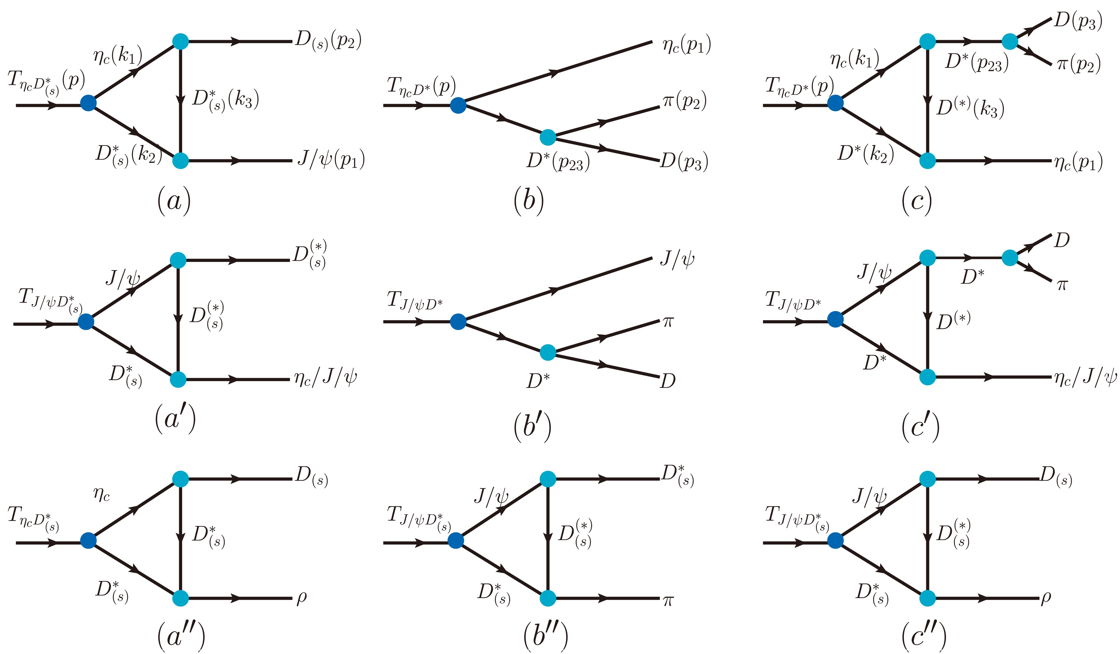
Figure 2. (color online) Diagrams (a,
$ a^\prime $ ,$ a^{\prime \prime} $ ,$ b^{\prime \prime} $ ,$ c^{\prime \prime} $ ) represent two-body decays of the molecular states$ T_{\eta_c D^*} $ and$ T_{J/\psi D^*} $ . Among them, the decay processes depicted in diagrams (a,$ a^\prime $ ) are dominant and are the primary focus of this paper, whereas those in diagrams ($ a^{\prime \prime} $ ,$ b^{\prime \prime} $ ,$ c^{\prime \prime} $ ) are suppressed. Diagrams (b,$ b^\prime $ ) and (c,$ c^\prime $ ) depict tree-level and one-loop three-body decays of the molecular states ($ T_{\eta_c D^*} $ and$ T_{J/\psi D^*} $ ), respectively.$\begin{aligned}[b] {{\cal{M}}^{\prime}}^{a}_{T_{\eta_c D^*}\to{J/\psi} D} =\;& \int \frac{{\rm d}^4k_{{ 3}}}{(2\pi)^4}g_{{ \eta_cD^*D }}g_{{ T_{\eta_c D^*}}}g_{{ J/\psi D^*D^* }}\frac{(-g^{m \mu}+\dfrac{k_3^m k_2^\mu}{m^2_{D^*}})(-g^{n \rho}+\dfrac{k_2^n k_2^\rho}{m_{D^*}^2}) \varepsilon_{\rho}(p) \varepsilon^{* a}(p_1)}{-(k_{{ 1}}^2-m_{{ \eta_c}}^2)\ (k_{{ 2}}^2-m_{{ D^*}}^2)\ (k_{{ 3}}^2-m_{{ D^*}}^2)}{\cal{F}}_2(k_3^2) \\& \times {(k_1+p_2)}_{\mu}(-{\rm i} {k_2}_{n} g_{am}+ {\rm i} k_{3a} g_{m n}- {\rm i} {k_2}_{m} g_{an}- {\rm i} {k_2}_{n} g_{m a}+ {\rm i} {p_1}_{a} g_{n m}- {\rm i} {p_1}_{ m} g_{n a}), \\ {{\cal{M}}^{\prime}}^{a^\prime}_{T_{J/\psi D^*}\to{J/\psi} D} =\;& \int \frac{{\rm d}^4k_{{ 3}}}{(2\pi)^4}g_{{ T_{J/\psi D^*}}}\Bigg\{g_{{ D^*D^* J/\psi }}g_{{ J/\psi D^*D }}\frac{(-g^{\beta m}+\dfrac{k_3^\beta k_3^m}{m_{D^*}^2})(-g^{\xi n}+\dfrac{k_2^n k_2^{\xi}}{m_{D^*}^2})(-g^{\rho \nu}+\dfrac{k_1^\rho k_1^\nu}{m_{J/\psi}^{2}})}{(k_{{ 1}}^2-m_{{ J/\psi}}^2)\ (k_{{ 2}}^2-m_{{ D^*}}^2)\ (k_{{ 3}}^2-m_{{ D}}^2)}\\ & \times (-{k_2}_{n} g_{a m}+{k_3}_{a}g_{m n}-k_{2 m} g_{a n}+{k_2}_{n} g_{m a}+{p_1}_{a} g_{n m}-{p_1}_{ m} g_{n a}){\cal{F}}_2(k_3^2)\varepsilon_{\mu \nu \alpha \beta} \varepsilon_{\gamma\sigma\rho\xi} \varepsilon^{\sigma}(p)\varepsilon^{* a}(p_1) k_1^\mu k_3^\alpha p^\gamma \\& +g_{{ \eta_cD^*D }}g_{{ J/\psi DD }}\varepsilon^{* \nu} (p_1){\cal{F}}_2(k_3^2) \frac{(-g^{\beta \xi}+\dfrac{k_2^\beta k_2^\xi}{m^2_{D^*}})(-g^{\mu \rho}+\dfrac{k_1^\mu k_1^\rho}{m_{J/\psi}^2})}{(k_{{ 1}}^2-m_{{ J/\psi}}^2)\ (k_{{ 2}}^2-m_{{ D^*}}^2)\ (k_{{ 3}}^2-m_{{ D}}^2)} p_1^\mu k_2^\alpha \varepsilon^\sigma(p) \varepsilon_{\gamma \sigma \rho \xi} \varepsilon_{\mu \nu \alpha \beta}{(k_3-p_2)}_ {\mu} p^\gamma\Bigg\},\\ {{\cal{M}}^{\prime}}^{a^\prime}_{T_{J/\psi D^*}\to{\eta_c D^*}}=\;& \int \frac{{\rm d}^4k_{{ 3}}}{(2\pi)^4}g_{{ T_{J/\psi D^*}}}\Bigg\{g_{{ \eta_cD^*D }}g_{{ J/\psi DD }}\frac{(-g_{\mu \rho}+\dfrac{k_2^\mu k_2^p}{m_{D^*}^2})(-i p^\sigma) \varepsilon_{\sigma \nu \alpha \rho}(-g^{\alpha \gamma}+\dfrac{k_1^\alpha k_1^\gamma}{m_{J/\psi}^2})}{(k_{{ 1}}^2-m_{{ J/\psi}}^2)\ (k_{{ 2}}^2-m_{{ D^*}}^2)\ (k_{{ 3}}^2-m_{{ D}}^2)}{\cal{F}}_2(k_3^2) \\ & \times {(p_2+k_3)}_{\mu} k_1^m p_1^n \varepsilon^\nu(p) \varepsilon_{m A x} \varepsilon_{n \xi m \gamma} \varepsilon^{* \xi}(p_2)+ g_{{ \eta_cD^*D^* }}g_{{ J/\psi D^*D }}\varepsilon^{* n}(p_1){\cal{F}}_2(k_3^2)\\ & \times \frac{(-g_{a \xi}+ \dfrac{{k_3}_{a}{k_3}_{\xi}}{m^2_{D^*}})(-g_{\sigma \beta}+\dfrac{{k_2}_{\beta} {k_2}_{\sigma}}{m^2_{D^*}})(-g_{\rho m}+\dfrac{{k_1}_{\rho}k_{1 m}}{m_{J/\psi}^2}) } {{\rm i}(k_{{ 1}}^2-m_{{ J/\psi}}^2)\ (k_{{ 2}}^2-m_{{ D^*}}^2)\ (k_{{ 3}}^2-m_{{ D}}^2)} \varepsilon^{\mu \nu \alpha \beta} \varepsilon^{\gamma \xi \rho \sigma} p_\gamma {k_3}_{\gamma} {k_2}_{\alpha}\\ & \times (- {k_1}_{n} g^{a m}+ k_1^a g_n^m+ k_3^m g_n^a- {k_2}_{n} g^{a m}+ p_2^a g_n^m- p_2^m g_n^a)\Bigg\} , \\ {{\cal{M}}^{\prime}}^{b^{\prime}+c^{\prime}}_{T_{\eta_c D^*}\to \eta_c D\pi} =\;& g_{{ T_{\eta_c D^*}}}g_{{ D^* D\pi}} \frac{\varepsilon^{\mu}(p)\left(-g_{\mu \nu}+\dfrac{{p_{23}}_\mu{p_{23}}_{\nu}}{m^2_{D^*}}\right)\left(p_2-p_3\right)^\nu}{\left(p_{23}^2-m_{D^*}^2\right)} + \int \frac{d^4k_{{ 3}}}{(2\pi)^4}g_{{ T_{\eta_c D^*}}}\\ & \times \Bigg\{g^2_{{ \eta_c D^*D^*}}g_{{ D^* D \pi }}\varepsilon_n(p){\cal{F}}_2(k_3^2)\frac{ (-g^{\mu \nu}+\dfrac{p_{23}^\nu p_{23}^\mu}{m^2_{D^*}})(-g^{m n}+\dfrac{k_2^m k_2^n}{m_{D^*}^2})}{i(k_{{ 1}}^2-m_{{ \eta_c}}^2)\ (k_{{ 2}}^2-m_{{ D^*}}^2)\ (k_{{ 3}}^2-m_{{ D}}^2)} {( p_{2 }- p_{3})}_{\nu}{(k_1-k_3 )}_{\mu}){(k_{3 }-p_{1 })}_m \\&+ g^2_{{ \eta_c D^*D}}g_{{ D^* D \pi }}\varepsilon_{\sigma}(p)\varepsilon_{\xi n m \gamma} k_2^{\xi} k_3^m (p_2-p_3)_{\rho}{\cal{F}}_2(k_3^2)\varepsilon_{\mu\nu\alpha\beta}k_3^{\mu}p_{23}^{\alpha}\frac{ (-g^{\sigma n}+\dfrac{k_{2}^{\sigma}k_{2}^{n}}{m_{D^{*}}^2})(-g^{\nu \gamma}+\dfrac{k_{3}^{\nu} k_{3}^{\gamma}}{m_{D^{*}}^2}) (-g^{\beta \rho}+\dfrac{p_{23}^{\beta} p_{23}^{\rho}}{m_{D^{*}}^2})}{(k_{{ 1}}^2-m_{{ \eta_c }}^2)\ (k_{{ 2}}^2-m_{{ D^*}}^2)\ (k_{{ 3}}^2-m_{{ D^*}}^2)}\Bigg\}\,,\\ {{\cal{M}}^{\prime}}^{b+c}_{T_{J/\psi D^*}\to J/\psi D\pi} =\;& g_{{ T_{J/\psi D^*}}}g_{{ D^*D \pi }}\frac{\varepsilon^{\mu\nu\alpha\beta}\varepsilon_{\nu}(p)\varepsilon^{*}_{\alpha}(p_1)(-g_{\beta m}+\dfrac{{P_23}_{\beta} {P_23}_{m} }{m^2_{D^*}})p_\mu{(p_2-p_3)}^m}{\left(p_{23}^2-m_{D^*}^2\right)}\\ & + \int \frac{{\rm d}^4k_{{ 3}}}{(2\pi)^4}g_{{ T_{J/\psi D^*}}}\Bigg\{g_{{ J/\psi D^*D^*}}g_{{ \eta_c D^*D^*}}g_{{ D^* D \pi }} \varepsilon_{\alpha\beta \rho \sigma} p^{\alpha} \varepsilon ^ { \beta } ( p ) \varepsilon ^ { * a }({p_1}) (-g^{\rho \mu}+ \frac{k_1^{\rho}k_1^{\mu}}{m_{J/\psi}^2})\\ & \times (p_2-p_3)_{ \nu}{\cal{F}}_2(k_3^2)(-g^{\sigma n}+\dfrac{k_2^{\sigma} k_2^{n}}{m_{D^{*}}^2})\frac{ (-g^{\gamma \nu}+\dfrac{p_{23}^{\gamma}p_{23}^{\nu}}{m_{D^{*}}^2}) (-g^{m \xi}+\dfrac{k_{3}^{m}k_{3}^{\xi}}{m_{D^{*}}^2})} {{\rm i} (k_1^2-m_{J/\psi}^2)(k_2^2-m_{D^{*}}^2)(k_3^2-m_{D^{*}}^2)} ( {k_2}_{n} g_{a m}- {k_3}_{a}g_{m n}+{k_2}_{m} g_{a n}+ {k_2}_{n} g_{m a} \\& - {p_1}_{a}g_{n m}+ {p_1}_{m} g_{n a})((p _1+k_3)_{\gamma} g_{\xi \mu}-{(p_1+k_3)}_{\xi} g_{\gamma \mu}-{k_3}_{\mu} g_{\xi \gamma}+ {k_3}_{\gamma} g_{\xi \mu}- {p_1}_{\xi} g_{\gamma \mu}-{p_1}_{\mu} g_{\gamma \xi})+g_{{ J/\psi D^*D^*}}g_{{ \eta_c D^*D^*}}\\ & \times g_{{ D^* D \pi }} \varepsilon_{\alpha\beta \rho \sigma}\varepsilon_{n a m \mu} \varepsilon_{\zeta \xi r \gamma } p^{\alpha} \varepsilon ^ { \beta } ( p ) \varepsilon ^ { * a } ( p_{ 1 } )p^n_1 k^m_2\varepsilon ^ { * a } ( p_{ 1 } ) k^{\zeta}_1 p^r_{23} {(p_2-p_3)}_{\nu}{\cal{F}}^2(k_3^2)\\ \end{aligned} $
$ \begin{aligned}[b] & \times (-g^{\rho \xi}+ \frac{k_1^{\rho}k_1^{\xi}}{m_{J/\psi}^2})\frac{ (-g^{\sigma \mu}+\frac{k_2^{\sigma} k_2^{\nu}}{m_{D^{*}}^2})(-g^{\gamma \nu}+\frac{p_{23}^{\gamma}p_{23}^{\nu}}{m_{D^{*}}^2}) } {(k_1^2-m_{J/\psi}^2)(k_2^2-m_{D^{*}}^2)(k_3^2-m_{D}^2)}\Bigg\},\\ {{\cal{M}}^{\prime}}^{c^{\prime}}_{T_{J/\psi D^*}\to \eta_c D\pi} =\;& \int \frac{{\rm d}^4k_{{ 3}}}{(2\pi)^4}g_{{ T_{J/\psi D^*}}}g_{{ D^* D \pi }}\Bigg\{g_{{ J/\psi D^*D^*}}g_{{ \eta_c D^*D^*}}\frac{{\rm i}\varepsilon_{\xi \zeta \rho\sigma}\varepsilon^{\xi}(p)p^{\zeta}(-g^{\rho m}+\dfrac{k_1^{\rho}k_1^m}{m_{J/\psi}^2})}{(k_{{ 1}}^2-m_{{ J/\psi}}^2)\ (k_{{ 2}}^2-m_{{ D^*}}^2)\ (k_{{ 3}}^2-m_{{ D^*}}^2)}(-g^{\sigma \beta}+\frac{k_2^{\sigma}k_2^{\beta}}{m_{D^{*}}^2}){\cal{F}}_2(k_3^2) ((p_1+k_3)_{n} g_{am}\\&-(p_1+k_3)_{a} g_{n m} -{k_3}_{m} g_{n a}+ {k_2}_{n} g_{a m}- {p_1}_{a} g_{n m}-{p_1}_{ m} g_{n a})\varepsilon_{\mu\nu\alpha\beta}k_3^{\mu}k_2^{\alpha}(-g^{\nu a}+\frac{k_3^{\nu}k_3^{a}}{m_{D^{*}}^2})(-g^{n \gamma }+\frac{p_{23}^{n}p_{23}^{\gamma}}{m_{D^{*}}^2})(p_{23}-p_{3})_{\gamma})\\&+g_{{ J/\psi DD^*}}g_{{ \eta_c DD^*}}\varepsilon_{\rho\nu\alpha\beta}p_{23}^{\rho}k_1^{\alpha} {\cal{F}}_2(k_3^2){(p_{2}-p_{3})}_{\gamma} (p_1+k_3)_\mu \varepsilon_{m n \xi \sigma} \varepsilon^n(p) p^m \\& \times \frac{(-g^{\gamma\nu}+\dfrac{p_{23}^{\gamma}p_{23}^{\nu}}{m_{D^{*}}^2})(-g^{\beta \xi}+\dfrac{k_1^{\beta}k_1^{\xi}}{m_{J/\psi}^2})(-g^{\mu \sigma}+\dfrac{k_2^\mu k_2^\sigma}{m_{D^{*}}^2})}{i(k_{{ 1}}^2-m_{{ J/\psi}}^2)\ (k_{{ 2}}^2-m_{{ D^*}}^2)\ (k_{{ 3}}^2-m_{{ D}}^2)}\Bigg\}. \end{aligned} $
(20) The momentum conventions are illustrated in Fig. 2. Here,
$ p_{23} = p_2 + p_3 $ , and$ k_3 $ denotes the momentum of the exchanged particle. The partial decay width for the three-body process$ T_{J/\psi(/\eta_c) D^*} \to J/\psi(/\eta_c) D \pi $ is given by [59]:$ {\rm d} \Gamma = \frac{1}{(2 \pi)^3} \frac{1}{32 m^3_{{ T}}} \overline{|{\cal{M}}^{\prime}|^2} {\rm d} m_{12}^2 {\rm d} m_{23}^2. $
(21) $ {\cal{M}}^{\prime} $ denotes the decay amplitudes;$ m_{12} $ and$ m_{23} $ represent the invariant masses of the final-state$ J/\psi \pi $ (or$ \eta_c \pi $ ) and$ D \pi $ systems, respectively, defined as$ m^2_{12} = (p_1+p_2)^2 $ and$ m^2_{23} = (p_2+p_3)^2 $ . The limits for the outer integration variables$m_{23}^2 $ and$m_{12}^2 $ are given by:$ \begin{array}{l} (m_{23}^2)_{\min} = (m_2 + m_3)^2, \quad (m_{23}^2)_{\max} = (M - m_1)^2,\\ (m_{12}^2)_{\max} = (E_1^* + E_2^*)^2 - \left( \sqrt{{E_1^*}^2 - m_1^2} - \sqrt{{E_2^*}^2 - m_2^2} \right)^2,\\ (m_{12}^2)_{\min} = (E_1^* + E_2^*)^2 - \left( \sqrt{{E_1^*}^2 - m_1^2} + \sqrt{{E_2^*}^2 - m_2^2} \right)^2, \end{array} $
(22) where
$ E_1^* = ({M^2 - m_{23}^2 - m_1^2})/{2m_{23}} $ and$ E_2^* = (m_{23}^2 - m_3^2 + m_2^2)/{2m_{23}} $ , with$E_1^* $ and$E_2^* $ denoting the energies of the$ J/\psi $ (or$ \eta_c $ ) and the π, respectively, in the rest frame of the system with invariant mass$ m_{23} $ . -
Within the effective Lagrangian framework, we derive the decay processes of the molecular states
$ \eta_c D^* $ and$ J/\psi D^* $ ; the corresponding diagrams are presented in Fig. 2. In addition to the conventional two-body decays, we also investigate possible three-body decays, whose representative diagrams are also shown in Fig. 2. In this work, we discuss the contributions of three-body decays arising at one loop. The decay amplitudes$ {\cal{M}}^{\prime} $ for the molecular states$ T_{J/\psi D^*} $ and$ T_{\eta_c D^*} $ are given as follows:
Figure 2. (color online) Diagrams (a,
$ a^\prime $ ,$ a^{\prime \prime} $ ,$ b^{\prime \prime} $ ,$ c^{\prime \prime} $ ) represent two-body decays of the molecular states$ T_{\eta_c D^*} $ and$ T_{J/\psi D^*} $ . Among them, the decay processes depicted in diagrams (a,$ a^\prime $ ) are dominant and are the primary focus of this paper, whereas those in diagrams ($ a^{\prime \prime} $ ,$ b^{\prime \prime} $ ,$ c^{\prime \prime} $ ) are suppressed. Diagrams (b,$ b^\prime $ ) and (c,$ c^\prime $ ) depict tree-level and one-loop three-body decays of the molecular states ($ T_{\eta_c D^*} $ and$ T_{J/\psi D^*} $ ), respectively.$\begin{aligned}[b] {{\cal{M}}^{\prime}}^{a}_{T_{\eta_c D^*}\to{J/\psi} D} =\;& \int \frac{d^4k_{{ 3}}}{(2\pi)^4}g_{{ \eta_cD^*D }}g_{{ T_{\eta_c D^*}}}g_{{ J/\psi D^*D^* }}\frac{(-g^{m \mu}+\dfrac{k_3^m k_2^\mu}{m^2_{D^*}})(-g^{n \rho}+\dfrac{k_2^n k_2^\rho}{m_{D^*}^2}) \varepsilon_{\rho}(p) \varepsilon^{* a}(p_1)}{-(k_{{ 1}}^2-m_{{ \eta_c}}^2)\ (k_{{ 2}}^2-m_{{ D^*}}^2)\ (k_{{ 3}}^2-m_{{ D^*}}^2)}{\cal{F}}_2(k_3^2) \\& {(k_1+p_2)}_{\mu}(-i {k_2}_{n} g_{am}+i k_{3a} g_{m n}-i{k_2}_{m} g_{an}-i {k_2}_{n} g_{m a}+i {p_1}_{a} g_{n m}-i {p_1}_{ m} g_{n a}), \\ {{\cal{M}}^{\prime}}^{a^\prime}_{T_{J/\psi D^*}\to{J/\psi} D} =\;& \int \frac{d^4k_{{ 3}}}{(2\pi)^4}g_{{ T_{J/\psi D^*}}}\Big\{g_{{ D^*D^* J/\psi }}g_{{ J/\psi D^*D }}\frac{(-g^{\beta m}+\dfrac{k_3^\beta k_3^m}{m_{D^*}^2})(-g^{\xi n}+\dfrac{k_2^n k_2^{\xi}}{m_{D^*}^2})(-g^{\rho \nu}+\dfrac{k_1^\rho k_1^\nu}{m_{J/\psi}^{2}})}{(k_{{ 1}}^2-m_{{ J/\psi}}^2)\ (k_{{ 2}}^2-m_{{ D^*}}^2)\ (k_{{ 3}}^2-m_{{ D}}^2)}\\ & (-{k_2}_{n} g_{a m}+{k_3}_{a}g_{m n}-k_{2 m} g_{a n}+{k_2}_{n} g_{m a}+{p_1}_{a} g_{n m}-{p_1}_{ m} g_{n a}){\cal{F}}_2(k_3^2)\varepsilon_{\mu \nu \alpha \beta} \varepsilon_{\gamma\sigma\rho\xi} \varepsilon^{\sigma}(p)\varepsilon^{* a}(p_1) k_1^\mu k_3^\alpha p^\gamma \\& +g_{{ \eta_cD^*D }}g_{{ J/\psi DD }}\varepsilon^{* \nu} (p_1){\cal{F}}_2(k_3^2) \frac{(-g^{\beta \xi}+\dfrac{k_2^\beta k_2^\xi}{m^2_{D^*}})(-g^{\mu \rho}+\dfrac{k_1^\mu k_1^\rho}{m_{J/\psi}^2})}{(k_{{ 1}}^2-m_{{ J/\psi}}^2)\ (k_{{ 2}}^2-m_{{ D^*}}^2)\ (k_{{ 3}}^2-m_{{ D}}^2)} p_1^\mu k_2^\alpha \varepsilon^\sigma(p) \varepsilon_{\gamma \sigma \rho \xi} \varepsilon_{\mu \nu \alpha \beta}{(k_3-p_2)}_ {\mu} p^\gamma\Big\},\\ {{\cal{M}}^{\prime}}^{a^\prime}_{T_{J/\psi D^*}\to{\eta_c D^*}}=\;& \int \frac{d^4k_{{ 3}}}{(2\pi)^4}g_{{ T_{J/\psi D^*}}}\Big\{g_{{ \eta_cD^*D }}g_{{ J/\psi DD }}\frac{(-g_{\mu \rho}+\dfrac{k_2^\mu k_2^p}{m_{D^*}^2})(-i p^\sigma) \varepsilon_{\sigma \nu \alpha \rho}(-g^{\alpha \gamma}+\dfrac{k_1^\alpha k_1^\gamma}{m_{J/\psi}^2})}{(k_{{ 1}}^2-m_{{ J/\psi}}^2)\ (k_{{ 2}}^2-m_{{ D^*}}^2)\ (k_{{ 3}}^2-m_{{ D}}^2)}{\cal{F}}_2(k_3^2) \\ & {(p_2+k_3)}_{\mu} k_1^m p_1^n \varepsilon^\nu(p) \varepsilon_{m A x} \varepsilon_{n \xi m \gamma} \varepsilon^{* \xi}(p_2)+ g_{{ \eta_cD^*D^* }}g_{{ J/\psi D^*D }}\varepsilon^{* n}(p_1){\cal{F}}_2(k_3^2)\\ & \frac{(-g_{a \xi}+ \dfrac{{k_3}_{a}{k_3}_{\xi}}{m^2_{D^*}})(-g_{\sigma \beta}+\dfrac{{k_2}_{\beta} {k_2}_{\sigma}}{m^2_{D^*}})(-g_{\rho m}+\dfrac{{k_1}_{\rho}k_{1 m}}{m_{J/\psi}^2}) } {i(k_{{ 1}}^2-m_{{ J/\psi}}^2)\ (k_{{ 2}}^2-m_{{ D^*}}^2)\ (k_{{ 3}}^2-m_{{ D}}^2)} \varepsilon^{\mu \nu \alpha \beta} \varepsilon^{\gamma \xi \rho \sigma} p_\gamma {k_3}_{\gamma} {k_2}_{\alpha}\\ & (- {k_1}_{n} g^{a m}+ k_1^a g_n^m+ k_3^m g_n^a- {k_2}_{n} g^{a m}+ p_2^a g_n^m- p_2^m g_n^a)\Big\} , \\ {{\cal{M}}^{\prime}}^{b^{\prime}+c^{\prime}}_{T_{\eta_c D^*}\to \eta_c D\pi} =\;& g_{{ T_{\eta_c D^*}}}g_{{ D^* D\pi}} \frac{\varepsilon^{\mu}(p)\left(-g_{\mu \nu}+\dfrac{{p_{23}}_\mu{p_{23}}_{\nu}}{m^2_{D^*}}\right)\left(p_2-p_3\right)^\nu}{\left(p_{23}^2-m_{D^*}^2\right)} + \int \frac{d^4k_{{ 3}}}{(2\pi)^4}g_{{ T_{\eta_c D^*}}}\\ & \Bigg\{g^2_{{ \eta_c D^*D^*}}g_{{ D^* D \pi }}\varepsilon_n(p){\cal{F}}_2(k_3^2)\frac{ (-g^{\mu \nu}+\dfrac{p_{23}^\nu p_{23}^\mu}{m^2_{D^*}})(-g^{m n}+\dfrac{k_2^m k_2^n}{m_{D^*}^2})}{i(k_{{ 1}}^2-m_{{ \eta_c}}^2)\ (k_{{ 2}}^2-m_{{ D^*}}^2)\ (k_{{ 3}}^2-m_{{ D}}^2)} {( p_{2 }- p_{3})}_{\nu}{(k_1-k_3 )}_{\mu}){(k_{3 }-p_{1 })}_m \\&+ g^2_{{ \eta_c D^*D}}g_{{ D^* D \pi }}\varepsilon_{\sigma}(p)\varepsilon_{\xi n m \gamma} k_2^{\xi} k_3^m (p_2-p_3)_{\rho}{\cal{F}}_2(k_3^2)\varepsilon_{\mu\nu\alpha\beta}k_3^{\mu}p_{23}^{\alpha}\frac{ (-g^{\sigma n}+\dfrac{k_{2}^{\sigma}k_{2}^{n}}{m_{D^{*}}^2})(-g^{\nu \gamma}+\dfrac{k_{3}^{\nu} k_{3}^{\gamma}}{m_{D^{*}}^2}) (-g^{\beta \rho}+\dfrac{p_{23}^{\beta} p_{23}^{\rho}}{m_{D^{*}}^2})}{(k_{{ 1}}^2-m_{{ \eta_c }}^2)\ (k_{{ 2}}^2-m_{{ D^*}}^2)\ (k_{{ 3}}^2-m_{{ D^*}}^2)}\Bigg\}\,,\\ {{\cal{M}}^{\prime}}^{b+c}_{T_{J/\psi D^*}\to J/\psi D\pi} =\;& g_{{ T_{J/\psi D^*}}}g_{{ D^*D \pi }}\frac{\varepsilon^{\mu\nu\alpha\beta}\varepsilon_{\nu}(p)\varepsilon^{*}_{\alpha}(p_1)(-g_{\beta m}+\dfrac{{P_23}_{\beta} {P_23}_{m} }{m^2_{D^*}})p_\mu{(p_2-p_3)}^m}{\left(p_{23}^2-m_{D^*}^2\right)}\\ & + \int \frac{d^4k_{{ 3}}}{(2\pi)^4}g_{{ T_{J/\psi D^*}}}\Bigg\{g_{{ J/\psi D^*D^*}}g_{{ \eta_c D^*D^*}}g_{{ D^* D \pi }} \varepsilon_{\alpha\beta \rho \sigma} p^{\alpha} \varepsilon ^ { \beta } ( p ) \varepsilon ^ { * a }({p_1}) (-g^{\rho \mu}+ \frac{k_1^{\rho}k_1^{\mu}}{m_{J/\psi}^2})\\ &(p_2-p_3)_{ \nu}{\cal{F}}_2(k_3^2)(-g^{\sigma n}+\dfrac{k_2^{\sigma} k_2^{n}}{m_{D^{*}}^2})\frac{ (-g^{\gamma \nu}+\dfrac{p_{23}^{\gamma}p_{23}^{\nu}}{m_{D^{*}}^2}) (-g^{m \xi}+\dfrac{k_{3}^{m}k_{3}^{\xi}}{m_{D^{*}}^2})} {i(k_1^2-m_{J/\psi}^2)(k_2^2-m_{D^{*}}^2)(k_3^2-m_{D^{*}}^2)} ( {k_2}_{n} g_{a m}- {k_3}_{a}g_{m n}+{k_2}_{m} g_{a n}+ {k_2}_{n} g_{m a} \\& - {p_1}_{a}g_{n m}+ {p_1}_{m} g_{n a})((p _1+k_3)_{\gamma} g_{\xi \mu}-{(p_1+k_3)}_{\xi} g_{\gamma \mu}-{k_3}_{\mu} g_{\xi \gamma}+ {k_3}_{\gamma} g_{\xi \mu}- {p_1}_{\xi} g_{\gamma \mu}-{p_1}_{\mu} g_{\gamma \xi})+g_{{ J/\psi D^*D^*}}g_{{ \eta_c D^*D^*}}\\ & g_{{ D^* D \pi }} \varepsilon_{\alpha\beta \rho \sigma}\varepsilon_{n a m \mu} \varepsilon_{\zeta \xi r \gamma } p^{\alpha} \varepsilon ^ { \beta } ( p ) \varepsilon ^ { * a } ( p_{ 1 } )p^n_1 k^m_2\varepsilon ^ { * a } ( p_{ 1 } ) k^{\zeta}_1 p^r_{23} {(p_2-p_3)}_{\nu}{\cal{F}}^2(k_3^2)\\ \end{aligned} $
$ \begin{aligned}[b] & (-g^{\rho \xi}+ \frac{k_1^{\rho}k_1^{\xi}}{m_{J/\psi}^2})\frac{ (-g^{\sigma \mu}+\frac{k_2^{\sigma} k_2^{\nu}}{m_{D^{*}}^2})(-g^{\gamma \nu}+\frac{p_{23}^{\gamma}p_{23}^{\nu}}{m_{D^{*}}^2}) } {(k_1^2-m_{J/\psi}^2)(k_2^2-m_{D^{*}}^2)(k_3^2-m_{D}^2)}\Bigg\},\\ {{\cal{M}}^{\prime}}^{c^{\prime}}_{T_{J/\psi D^*}\to \eta_c D\pi} =\;& \int \frac{d^4k_{{ 3}}}{(2\pi)^4}g_{{ T_{J/\psi D^*}}}g_{{ D^* D \pi }}\Bigg\{g_{{ J/\psi D^*D^*}}g_{{ \eta_c D^*D^*}}\frac{i\varepsilon_{\xi \zeta \rho\sigma}\varepsilon^{\xi}(p)p^{\zeta}(-g^{\rho m}+\dfrac{k_1^{\rho}k_1^m}{m_{J/\psi}^2})}{(k_{{ 1}}^2-m_{{ J/\psi}}^2)\ (k_{{ 2}}^2-m_{{ D^*}}^2)\ (k_{{ 3}}^2-m_{{ D^*}}^2)}(-g^{\sigma \beta}+\frac{k_2^{\sigma}k_2^{\beta}}{m_{D^{*}}^2}){\cal{F}}_2(k_3^2) ((p_1+k_3)_{n} g_{am}\\&-(p_1+k_3)_{a} g_{n m} -{k_3}_{m} g_{n a}+ {k_2}_{n} g_{a m}- {p_1}_{a} g_{n m}-{p_1}_{ m} g_{n a})\varepsilon_{\mu\nu\alpha\beta}k_3^{\mu}k_2^{\alpha}(-g^{\nu a}+\frac{k_3^{\nu}k_3^{a}}{m_{D^{*}}^2})(-g^{n \gamma }+\frac{p_{23}^{n}p_{23}^{\gamma}}{m_{D^{*}}^2})(p_{23}-p_{3})_{\gamma})\\&+g_{{ J/\psi DD^*}}g_{{ \eta_c DD^*}}\varepsilon_{\rho\nu\alpha\beta}p_{23}^{\rho}k_1^{\alpha} {\cal{F}}_2(k_3^2){(p_{2}-p_{3})}_{\gamma} (p_1+k_3)_\mu \varepsilon_{m n \xi \sigma} \varepsilon^n(p) p^m \\&\frac{(-g^{\gamma\nu}+\dfrac{p_{23}^{\gamma}p_{23}^{\nu}}{m_{D^{*}}^2})(-g^{\beta \xi}+\dfrac{k_1^{\beta}k_1^{\xi}}{m_{J/\psi}^2})(-g^{\mu \sigma}+\dfrac{k_2^\mu k_2^\sigma}{m_{D^{*}}^2})}{i(k_{{ 1}}^2-m_{{ J/\psi}}^2)\ (k_{{ 2}}^2-m_{{ D^*}}^2)\ (k_{{ 3}}^2-m_{{ D}}^2)}\Bigg\}. \end{aligned} $
(20) The momentum conventions are illustrated in Fig. 2. Here,
$ p_{23} = p_2 + p_3 $ , and$ k_3 $ denotes the momentum of the exchanged particle. The partial decay width for the three-body process$ T_{J/\psi(/\eta_c) D^*} \to J/\psi(/\eta_c) D \pi $ is given by [60]:$ d \Gamma = \frac{1}{(2 \pi)^3} \frac{1}{32 m^3_{{ T}}} \overline{|{\cal{M}}^{\prime}|^2} d m_{12}^2 d m_{23}^2. $
(21) $ {\cal{M}}^{\prime} $ denotes the decay amplitudes;$ m_{12} $ and$ m_{23} $ represent the invariant masses of the final-state$ J/\psi \pi $ (or$ \eta_c \pi $ ) and$ D \pi $ systems, respectively, defined as$ m^2_{12} = (p_1+p_2)^2 $ and$ m^2_{23} = (p_2+p_3)^2 $ . The limits for the outer integration variables$m_{23}^2 $ and$m_{12}^2 $ are given by:$ \begin{array}{l} (m_{23}^2)_{\min} = (m_2 + m_3)^2, \quad (m_{23}^2)_{\max} = (M - m_1)^2,\\ (m_{12}^2)_{\max} = (E_1^* + E_2^*)^2 - \left( \sqrt{{E_1^*}^2 - m_1^2} - \sqrt{{E_2^*}^2 - m_2^2} \right)^2,\\ (m_{12}^2)_{\min} = (E_1^* + E_2^*)^2 - \left( \sqrt{{E_1^*}^2 - m_1^2} + \sqrt{{E_2^*}^2 - m_2^2} \right)^2, \end{array} $
(22) where
$ E_1^* = ({M^2 - m_{23}^2 - m_1^2})/{2m_{23}} $ and$ E_2^* = (m_{23}^2 - m_3^2 + m_2^2)/{2m_{23}} $ , with$E_1^* $ and$E_2^* $ denoting the energies of the$ J/\psi $ (or$ \eta_c $ ) and the π, respectively, in the rest frame of the system with invariant mass$ m_{23} $ . -
Within the effective Lagrangian framework, we derive the decay processes of the molecular states
$ \eta_c D^* $ and$ J/\psi D^* $ ; the corresponding diagrams are presented in Fig. 2. In addition to the conventional two-body decays, we also investigate possible three-body decays, whose representative diagrams are also shown in Fig. 2. In this work, we discuss the contributions of three-body decays arising at one loop. The decay amplitudes$ {\cal{M}}^{\prime} $ for the molecular states$ T_{J/\psi D^*} $ and$ T_{\eta_c D^*} $ are given as follows:
Figure 2. (color online) Diagrams (a,
$ a^\prime $ ,$ a^{\prime \prime} $ ,$ b^{\prime \prime} $ ,$ c^{\prime \prime} $ ) represent two-body decays of the molecular states$ T_{\eta_c D^*} $ and$ T_{J/\psi D^*} $ . Among them, the decay processes depicted in diagrams (a,$ a^\prime $ ) are dominant and are the primary focus of this paper, whereas those in diagrams ($ a^{\prime \prime} $ ,$ b^{\prime \prime} $ ,$ c^{\prime \prime} $ ) are suppressed. Diagrams (b,$ b^\prime $ ) and (c,$ c^\prime $ ) depict tree-level and one-loop three-body decays of the molecular states ($ T_{\eta_c D^*} $ and$ T_{J/\psi D^*} $ ), respectively.$\begin{aligned}[b] {{\cal{M}}^{\prime}}^{a}_{T_{\eta_c D^*}\to{J/\psi} D} =\;& \int \frac{{\rm d}^4k_{{ 3}}}{(2\pi)^4}g_{{ \eta_cD^*D }}g_{{ T_{\eta_c D^*}}}g_{{ J/\psi D^*D^* }}\frac{(-g^{m \mu}+\dfrac{k_3^m k_2^\mu}{m^2_{D^*}})(-g^{n \rho}+\dfrac{k_2^n k_2^\rho}{m_{D^*}^2}) \varepsilon_{\rho}(p) \varepsilon^{* a}(p_1)}{-(k_{{ 1}}^2-m_{{ \eta_c}}^2)\ (k_{{ 2}}^2-m_{{ D^*}}^2)\ (k_{{ 3}}^2-m_{{ D^*}}^2)}{\cal{F}}_2(k_3^2) \\& \times {(k_1+p_2)}_{\mu}(-{\rm i} {k_2}_{n} g_{am}+ {\rm i} k_{3a} g_{m n}- {\rm i} {k_2}_{m} g_{an}- {\rm i} {k_2}_{n} g_{m a}+ {\rm i} {p_1}_{a} g_{n m}- {\rm i} {p_1}_{ m} g_{n a}), \\ {{\cal{M}}^{\prime}}^{a^\prime}_{T_{J/\psi D^*}\to{J/\psi} D} =\;& \int \frac{{\rm d}^4k_{{ 3}}}{(2\pi)^4}g_{{ T_{J/\psi D^*}}}\Bigg\{g_{{ D^*D^* J/\psi }}g_{{ J/\psi D^*D }}\frac{(-g^{\beta m}+\dfrac{k_3^\beta k_3^m}{m_{D^*}^2})(-g^{\xi n}+\dfrac{k_2^n k_2^{\xi}}{m_{D^*}^2})(-g^{\rho \nu}+\dfrac{k_1^\rho k_1^\nu}{m_{J/\psi}^{2}})}{(k_{{ 1}}^2-m_{{ J/\psi}}^2)\ (k_{{ 2}}^2-m_{{ D^*}}^2)\ (k_{{ 3}}^2-m_{{ D}}^2)}\\ & \times (-{k_2}_{n} g_{a m}+{k_3}_{a}g_{m n}-k_{2 m} g_{a n}+{k_2}_{n} g_{m a}+{p_1}_{a} g_{n m}-{p_1}_{ m} g_{n a}){\cal{F}}_2(k_3^2)\varepsilon_{\mu \nu \alpha \beta} \varepsilon_{\gamma\sigma\rho\xi} \varepsilon^{\sigma}(p)\varepsilon^{* a}(p_1) k_1^\mu k_3^\alpha p^\gamma \\& +g_{{ \eta_cD^*D }}g_{{ J/\psi DD }}\varepsilon^{* \nu} (p_1){\cal{F}}_2(k_3^2) \frac{(-g^{\beta \xi}+\dfrac{k_2^\beta k_2^\xi}{m^2_{D^*}})(-g^{\mu \rho}+\dfrac{k_1^\mu k_1^\rho}{m_{J/\psi}^2})}{(k_{{ 1}}^2-m_{{ J/\psi}}^2)\ (k_{{ 2}}^2-m_{{ D^*}}^2)\ (k_{{ 3}}^2-m_{{ D}}^2)} p_1^\mu k_2^\alpha \varepsilon^\sigma(p) \varepsilon_{\gamma \sigma \rho \xi} \varepsilon_{\mu \nu \alpha \beta}{(k_3-p_2)}_ {\mu} p^\gamma\Bigg\},\\ {{\cal{M}}^{\prime}}^{a^\prime}_{T_{J/\psi D^*}\to{\eta_c D^*}}=\;& \int \frac{{\rm d}^4k_{{ 3}}}{(2\pi)^4}g_{{ T_{J/\psi D^*}}}\Bigg\{g_{{ \eta_cD^*D }}g_{{ J/\psi DD }}\frac{(-g_{\mu \rho}+\dfrac{k_2^\mu k_2^p}{m_{D^*}^2})(-i p^\sigma) \varepsilon_{\sigma \nu \alpha \rho}(-g^{\alpha \gamma}+\dfrac{k_1^\alpha k_1^\gamma}{m_{J/\psi}^2})}{(k_{{ 1}}^2-m_{{ J/\psi}}^2)\ (k_{{ 2}}^2-m_{{ D^*}}^2)\ (k_{{ 3}}^2-m_{{ D}}^2)}{\cal{F}}_2(k_3^2) \\ & \times {(p_2+k_3)}_{\mu} k_1^m p_1^n \varepsilon^\nu(p) \varepsilon_{m A x} \varepsilon_{n \xi m \gamma} \varepsilon^{* \xi}(p_2)+ g_{{ \eta_cD^*D^* }}g_{{ J/\psi D^*D }}\varepsilon^{* n}(p_1){\cal{F}}_2(k_3^2)\\ & \times \frac{(-g_{a \xi}+ \dfrac{{k_3}_{a}{k_3}_{\xi}}{m^2_{D^*}})(-g_{\sigma \beta}+\dfrac{{k_2}_{\beta} {k_2}_{\sigma}}{m^2_{D^*}})(-g_{\rho m}+\dfrac{{k_1}_{\rho}k_{1 m}}{m_{J/\psi}^2}) } {{\rm i}(k_{{ 1}}^2-m_{{ J/\psi}}^2)\ (k_{{ 2}}^2-m_{{ D^*}}^2)\ (k_{{ 3}}^2-m_{{ D}}^2)} \varepsilon^{\mu \nu \alpha \beta} \varepsilon^{\gamma \xi \rho \sigma} p_\gamma {k_3}_{\gamma} {k_2}_{\alpha}\\ & \times (- {k_1}_{n} g^{a m}+ k_1^a g_n^m+ k_3^m g_n^a- {k_2}_{n} g^{a m}+ p_2^a g_n^m- p_2^m g_n^a)\Bigg\} , \\ {{\cal{M}}^{\prime}}^{b^{\prime}+c^{\prime}}_{T_{\eta_c D^*}\to \eta_c D\pi} =\;& g_{{ T_{\eta_c D^*}}}g_{{ D^* D\pi}} \frac{\varepsilon^{\mu}(p)\left(-g_{\mu \nu}+\dfrac{{p_{23}}_\mu{p_{23}}_{\nu}}{m^2_{D^*}}\right)\left(p_2-p_3\right)^\nu}{\left(p_{23}^2-m_{D^*}^2\right)} + \int \frac{d^4k_{{ 3}}}{(2\pi)^4}g_{{ T_{\eta_c D^*}}}\\ & \times \Bigg\{g^2_{{ \eta_c D^*D^*}}g_{{ D^* D \pi }}\varepsilon_n(p){\cal{F}}_2(k_3^2)\frac{ (-g^{\mu \nu}+\dfrac{p_{23}^\nu p_{23}^\mu}{m^2_{D^*}})(-g^{m n}+\dfrac{k_2^m k_2^n}{m_{D^*}^2})}{i(k_{{ 1}}^2-m_{{ \eta_c}}^2)\ (k_{{ 2}}^2-m_{{ D^*}}^2)\ (k_{{ 3}}^2-m_{{ D}}^2)} {( p_{2 }- p_{3})}_{\nu}{(k_1-k_3 )}_{\mu}){(k_{3 }-p_{1 })}_m \\&+ g^2_{{ \eta_c D^*D}}g_{{ D^* D \pi }}\varepsilon_{\sigma}(p)\varepsilon_{\xi n m \gamma} k_2^{\xi} k_3^m (p_2-p_3)_{\rho}{\cal{F}}_2(k_3^2)\varepsilon_{\mu\nu\alpha\beta}k_3^{\mu}p_{23}^{\alpha}\frac{ (-g^{\sigma n}+\dfrac{k_{2}^{\sigma}k_{2}^{n}}{m_{D^{*}}^2})(-g^{\nu \gamma}+\dfrac{k_{3}^{\nu} k_{3}^{\gamma}}{m_{D^{*}}^2}) (-g^{\beta \rho}+\dfrac{p_{23}^{\beta} p_{23}^{\rho}}{m_{D^{*}}^2})}{(k_{{ 1}}^2-m_{{ \eta_c }}^2)\ (k_{{ 2}}^2-m_{{ D^*}}^2)\ (k_{{ 3}}^2-m_{{ D^*}}^2)}\Bigg\}\,,\\ {{\cal{M}}^{\prime}}^{b+c}_{T_{J/\psi D^*}\to J/\psi D\pi} =\;& g_{{ T_{J/\psi D^*}}}g_{{ D^*D \pi }}\frac{\varepsilon^{\mu\nu\alpha\beta}\varepsilon_{\nu}(p)\varepsilon^{*}_{\alpha}(p_1)(-g_{\beta m}+\dfrac{{P_23}_{\beta} {P_23}_{m} }{m^2_{D^*}})p_\mu{(p_2-p_3)}^m}{\left(p_{23}^2-m_{D^*}^2\right)}\\ & + \int \frac{{\rm d}^4k_{{ 3}}}{(2\pi)^4}g_{{ T_{J/\psi D^*}}}\Bigg\{g_{{ J/\psi D^*D^*}}g_{{ \eta_c D^*D^*}}g_{{ D^* D \pi }} \varepsilon_{\alpha\beta \rho \sigma} p^{\alpha} \varepsilon ^ { \beta } ( p ) \varepsilon ^ { * a }({p_1}) (-g^{\rho \mu}+ \frac{k_1^{\rho}k_1^{\mu}}{m_{J/\psi}^2})\\ & \times (p_2-p_3)_{ \nu}{\cal{F}}_2(k_3^2)(-g^{\sigma n}+\dfrac{k_2^{\sigma} k_2^{n}}{m_{D^{*}}^2})\frac{ (-g^{\gamma \nu}+\dfrac{p_{23}^{\gamma}p_{23}^{\nu}}{m_{D^{*}}^2}) (-g^{m \xi}+\dfrac{k_{3}^{m}k_{3}^{\xi}}{m_{D^{*}}^2})} {{\rm i} (k_1^2-m_{J/\psi}^2)(k_2^2-m_{D^{*}}^2)(k_3^2-m_{D^{*}}^2)} ( {k_2}_{n} g_{a m}- {k_3}_{a}g_{m n}+{k_2}_{m} g_{a n}+ {k_2}_{n} g_{m a} \\& - {p_1}_{a}g_{n m}+ {p_1}_{m} g_{n a})((p _1+k_3)_{\gamma} g_{\xi \mu}-{(p_1+k_3)}_{\xi} g_{\gamma \mu}-{k_3}_{\mu} g_{\xi \gamma}+ {k_3}_{\gamma} g_{\xi \mu}- {p_1}_{\xi} g_{\gamma \mu}-{p_1}_{\mu} g_{\gamma \xi})+g_{{ J/\psi D^*D^*}}g_{{ \eta_c D^*D^*}}\\ & \times g_{{ D^* D \pi }} \varepsilon_{\alpha\beta \rho \sigma}\varepsilon_{n a m \mu} \varepsilon_{\zeta \xi r \gamma } p^{\alpha} \varepsilon ^ { \beta } ( p ) \varepsilon ^ { * a } ( p_{ 1 } )p^n_1 k^m_2\varepsilon ^ { * a } ( p_{ 1 } ) k^{\zeta}_1 p^r_{23} {(p_2-p_3)}_{\nu}{\cal{F}}^2(k_3^2)\\ \end{aligned} $
$ \begin{aligned}[b] & \times (-g^{\rho \xi}+ \frac{k_1^{\rho}k_1^{\xi}}{m_{J/\psi}^2})\frac{ (-g^{\sigma \mu}+\frac{k_2^{\sigma} k_2^{\nu}}{m_{D^{*}}^2})(-g^{\gamma \nu}+\frac{p_{23}^{\gamma}p_{23}^{\nu}}{m_{D^{*}}^2}) } {(k_1^2-m_{J/\psi}^2)(k_2^2-m_{D^{*}}^2)(k_3^2-m_{D}^2)}\Bigg\},\\ {{\cal{M}}^{\prime}}^{c^{\prime}}_{T_{J/\psi D^*}\to \eta_c D\pi} =\;& \int \frac{{\rm d}^4k_{{ 3}}}{(2\pi)^4}g_{{ T_{J/\psi D^*}}}g_{{ D^* D \pi }}\Bigg\{g_{{ J/\psi D^*D^*}}g_{{ \eta_c D^*D^*}}\frac{{\rm i}\varepsilon_{\xi \zeta \rho\sigma}\varepsilon^{\xi}(p)p^{\zeta}(-g^{\rho m}+\dfrac{k_1^{\rho}k_1^m}{m_{J/\psi}^2})}{(k_{{ 1}}^2-m_{{ J/\psi}}^2)\ (k_{{ 2}}^2-m_{{ D^*}}^2)\ (k_{{ 3}}^2-m_{{ D^*}}^2)}(-g^{\sigma \beta}+\frac{k_2^{\sigma}k_2^{\beta}}{m_{D^{*}}^2}){\cal{F}}_2(k_3^2) ((p_1+k_3)_{n} g_{am}\\&-(p_1+k_3)_{a} g_{n m} -{k_3}_{m} g_{n a}+ {k_2}_{n} g_{a m}- {p_1}_{a} g_{n m}-{p_1}_{ m} g_{n a})\varepsilon_{\mu\nu\alpha\beta}k_3^{\mu}k_2^{\alpha}(-g^{\nu a}+\frac{k_3^{\nu}k_3^{a}}{m_{D^{*}}^2})(-g^{n \gamma }+\frac{p_{23}^{n}p_{23}^{\gamma}}{m_{D^{*}}^2})(p_{23}-p_{3})_{\gamma})\\&+g_{{ J/\psi DD^*}}g_{{ \eta_c DD^*}}\varepsilon_{\rho\nu\alpha\beta}p_{23}^{\rho}k_1^{\alpha} {\cal{F}}_2(k_3^2){(p_{2}-p_{3})}_{\gamma} (p_1+k_3)_\mu \varepsilon_{m n \xi \sigma} \varepsilon^n(p) p^m \\& \times \frac{(-g^{\gamma\nu}+\dfrac{p_{23}^{\gamma}p_{23}^{\nu}}{m_{D^{*}}^2})(-g^{\beta \xi}+\dfrac{k_1^{\beta}k_1^{\xi}}{m_{J/\psi}^2})(-g^{\mu \sigma}+\dfrac{k_2^\mu k_2^\sigma}{m_{D^{*}}^2})}{i(k_{{ 1}}^2-m_{{ J/\psi}}^2)\ (k_{{ 2}}^2-m_{{ D^*}}^2)\ (k_{{ 3}}^2-m_{{ D}}^2)}\Bigg\}. \end{aligned} $
(20) The momentum conventions are illustrated in Fig. 2. Here,
$ p_{23} = p_2 + p_3 $ , and$ k_3 $ denotes the momentum of the exchanged particle. The partial decay width for the three-body process$ T_{J/\psi(/\eta_c) D^*} \to J/\psi(/\eta_c) D \pi $ is given by [59]:$ {\rm d} \Gamma = \frac{1}{(2 \pi)^3} \frac{1}{32 m^3_{{ T}}} \overline{|{\cal{M}}^{\prime}|^2} {\rm d} m_{12}^2 {\rm d} m_{23}^2. $
(21) $ {\cal{M}}^{\prime} $ denotes the decay amplitudes;$ m_{12} $ and$ m_{23} $ represent the invariant masses of the final-state$ J/\psi \pi $ (or$ \eta_c \pi $ ) and$ D \pi $ systems, respectively, defined as$ m^2_{12} = (p_1+p_2)^2 $ and$ m^2_{23} = (p_2+p_3)^2 $ . The limits for the outer integration variables$m_{23}^2 $ and$m_{12}^2 $ are given by:$ \begin{array}{l} (m_{23}^2)_{\min} = (m_2 + m_3)^2, \quad (m_{23}^2)_{\max} = (M - m_1)^2,\\ (m_{12}^2)_{\max} = (E_1^* + E_2^*)^2 - \left( \sqrt{{E_1^*}^2 - m_1^2} - \sqrt{{E_2^*}^2 - m_2^2} \right)^2,\\ (m_{12}^2)_{\min} = (E_1^* + E_2^*)^2 - \left( \sqrt{{E_1^*}^2 - m_1^2} + \sqrt{{E_2^*}^2 - m_2^2} \right)^2, \end{array} $
(22) where
$ E_1^* = ({M^2 - m_{23}^2 - m_1^2})/{2m_{23}} $ and$ E_2^* = (m_{23}^2 - m_3^2 + m_2^2)/{2m_{23}} $ , with$E_1^* $ and$E_2^* $ denoting the energies of the$ J/\psi $ (or$ \eta_c $ ) and the π, respectively, in the rest frame of the system with invariant mass$ m_{23} $ . -
Within the effective Lagrangian framework, we derive the decay processes of the molecular states
$ \eta_c D^* $ and$ J/\psi D^* $ ; the corresponding diagrams are presented in Fig. 2. In addition to the conventional two-body decays, we also investigate possible three-body decays, whose representative diagrams are also shown in Fig. 2. In this work, we discuss the contributions of three-body decays arising at one loop. The decay amplitudes$ {\cal{M}}^{\prime} $ for the molecular states$ T_{J/\psi D^*} $ and$ T_{\eta_c D^*} $ are given as follows:
Figure 2. (color online) Diagrams (a,
$ a^\prime $ ,$ a^{\prime \prime} $ ,$ b^{\prime \prime} $ ,$ c^{\prime \prime} $ ) represent two-body decays of the molecular states$ T_{\eta_c D^*} $ and$ T_{J/\psi D^*} $ . Among them, the decay processes depicted in diagrams (a,$ a^\prime $ ) are dominant and are the primary focus of this paper, whereas those in diagrams ($ a^{\prime \prime} $ ,$ b^{\prime \prime} $ ,$ c^{\prime \prime} $ ) are suppressed. Diagrams (b,$ b^\prime $ ) and (c,$ c^\prime $ ) depict tree-level and one-loop three-body decays of the molecular states ($ T_{\eta_c D^*} $ and$ T_{J/\psi D^*} $ ), respectively.$\begin{aligned}[b] {{\cal{M}}^{\prime}}^{a}_{T_{\eta_c D^*}\to{J/\psi} D} =\;& \int \frac{{\rm d}^4k_{{ 3}}}{(2\pi)^4}g_{{ \eta_cD^*D }}g_{{ T_{\eta_c D^*}}}g_{{ J/\psi D^*D^* }}\frac{(-g^{m \mu}+\dfrac{k_3^m k_2^\mu}{m^2_{D^*}})(-g^{n \rho}+\dfrac{k_2^n k_2^\rho}{m_{D^*}^2}) \varepsilon_{\rho}(p) \varepsilon^{* a}(p_1)}{-(k_{{ 1}}^2-m_{{ \eta_c}}^2)\ (k_{{ 2}}^2-m_{{ D^*}}^2)\ (k_{{ 3}}^2-m_{{ D^*}}^2)}{\cal{F}}_2(k_3^2) \\& \times {(k_1+p_2)}_{\mu}(-{\rm i} {k_2}_{n} g_{am}+ {\rm i} k_{3a} g_{m n}- {\rm i} {k_2}_{m} g_{an}- {\rm i} {k_2}_{n} g_{m a}+ {\rm i} {p_1}_{a} g_{n m}- {\rm i} {p_1}_{ m} g_{n a}), \\ {{\cal{M}}^{\prime}}^{a^\prime}_{T_{J/\psi D^*}\to{J/\psi} D} =\;& \int \frac{{\rm d}^4k_{{ 3}}}{(2\pi)^4}g_{{ T_{J/\psi D^*}}}\Bigg\{g_{{ D^*D^* J/\psi }}g_{{ J/\psi D^*D }}\frac{(-g^{\beta m}+\dfrac{k_3^\beta k_3^m}{m_{D^*}^2})(-g^{\xi n}+\dfrac{k_2^n k_2^{\xi}}{m_{D^*}^2})(-g^{\rho \nu}+\dfrac{k_1^\rho k_1^\nu}{m_{J/\psi}^{2}})}{(k_{{ 1}}^2-m_{{ J/\psi}}^2)\ (k_{{ 2}}^2-m_{{ D^*}}^2)\ (k_{{ 3}}^2-m_{{ D}}^2)}\\ & \times (-{k_2}_{n} g_{a m}+{k_3}_{a}g_{m n}-k_{2 m} g_{a n}+{k_2}_{n} g_{m a}+{p_1}_{a} g_{n m}-{p_1}_{ m} g_{n a}){\cal{F}}_2(k_3^2)\varepsilon_{\mu \nu \alpha \beta} \varepsilon_{\gamma\sigma\rho\xi} \varepsilon^{\sigma}(p)\varepsilon^{* a}(p_1) k_1^\mu k_3^\alpha p^\gamma \\& +g_{{ \eta_cD^*D }}g_{{ J/\psi DD }}\varepsilon^{* \nu} (p_1){\cal{F}}_2(k_3^2) \frac{(-g^{\beta \xi}+\dfrac{k_2^\beta k_2^\xi}{m^2_{D^*}})(-g^{\mu \rho}+\dfrac{k_1^\mu k_1^\rho}{m_{J/\psi}^2})}{(k_{{ 1}}^2-m_{{ J/\psi}}^2)\ (k_{{ 2}}^2-m_{{ D^*}}^2)\ (k_{{ 3}}^2-m_{{ D}}^2)} p_1^\mu k_2^\alpha \varepsilon^\sigma(p) \varepsilon_{\gamma \sigma \rho \xi} \varepsilon_{\mu \nu \alpha \beta}{(k_3-p_2)}_ {\mu} p^\gamma\Bigg\},\\ {{\cal{M}}^{\prime}}^{a^\prime}_{T_{J/\psi D^*}\to{\eta_c D^*}}=\;& \int \frac{{\rm d}^4k_{{ 3}}}{(2\pi)^4}g_{{ T_{J/\psi D^*}}}\Bigg\{g_{{ \eta_cD^*D }}g_{{ J/\psi DD }}\frac{(-g_{\mu \rho}+\dfrac{k_2^\mu k_2^p}{m_{D^*}^2})(-i p^\sigma) \varepsilon_{\sigma \nu \alpha \rho}(-g^{\alpha \gamma}+\dfrac{k_1^\alpha k_1^\gamma}{m_{J/\psi}^2})}{(k_{{ 1}}^2-m_{{ J/\psi}}^2)\ (k_{{ 2}}^2-m_{{ D^*}}^2)\ (k_{{ 3}}^2-m_{{ D}}^2)}{\cal{F}}_2(k_3^2) \\ & \times {(p_2+k_3)}_{\mu} k_1^m p_1^n \varepsilon^\nu(p) \varepsilon_{m A x} \varepsilon_{n \xi m \gamma} \varepsilon^{* \xi}(p_2)+ g_{{ \eta_cD^*D^* }}g_{{ J/\psi D^*D }}\varepsilon^{* n}(p_1){\cal{F}}_2(k_3^2)\\ & \times \frac{(-g_{a \xi}+ \dfrac{{k_3}_{a}{k_3}_{\xi}}{m^2_{D^*}})(-g_{\sigma \beta}+\dfrac{{k_2}_{\beta} {k_2}_{\sigma}}{m^2_{D^*}})(-g_{\rho m}+\dfrac{{k_1}_{\rho}k_{1 m}}{m_{J/\psi}^2}) } {{\rm i}(k_{{ 1}}^2-m_{{ J/\psi}}^2)\ (k_{{ 2}}^2-m_{{ D^*}}^2)\ (k_{{ 3}}^2-m_{{ D}}^2)} \varepsilon^{\mu \nu \alpha \beta} \varepsilon^{\gamma \xi \rho \sigma} p_\gamma {k_3}_{\gamma} {k_2}_{\alpha}\\ & \times (- {k_1}_{n} g^{a m}+ k_1^a g_n^m+ k_3^m g_n^a- {k_2}_{n} g^{a m}+ p_2^a g_n^m- p_2^m g_n^a)\Bigg\} , \\ {{\cal{M}}^{\prime}}^{b^{\prime}+c^{\prime}}_{T_{\eta_c D^*}\to \eta_c D\pi} =\;& g_{{ T_{\eta_c D^*}}}g_{{ D^* D\pi}} \frac{\varepsilon^{\mu}(p)\left(-g_{\mu \nu}+\dfrac{{p_{23}}_\mu{p_{23}}_{\nu}}{m^2_{D^*}}\right)\left(p_2-p_3\right)^\nu}{\left(p_{23}^2-m_{D^*}^2\right)} + \int \frac{d^4k_{{ 3}}}{(2\pi)^4}g_{{ T_{\eta_c D^*}}}\\ & \times \Bigg\{g^2_{{ \eta_c D^*D^*}}g_{{ D^* D \pi }}\varepsilon_n(p){\cal{F}}_2(k_3^2)\frac{ (-g^{\mu \nu}+\dfrac{p_{23}^\nu p_{23}^\mu}{m^2_{D^*}})(-g^{m n}+\dfrac{k_2^m k_2^n}{m_{D^*}^2})}{i(k_{{ 1}}^2-m_{{ \eta_c}}^2)\ (k_{{ 2}}^2-m_{{ D^*}}^2)\ (k_{{ 3}}^2-m_{{ D}}^2)} {( p_{2 }- p_{3})}_{\nu}{(k_1-k_3 )}_{\mu}){(k_{3 }-p_{1 })}_m \\&+ g^2_{{ \eta_c D^*D}}g_{{ D^* D \pi }}\varepsilon_{\sigma}(p)\varepsilon_{\xi n m \gamma} k_2^{\xi} k_3^m (p_2-p_3)_{\rho}{\cal{F}}_2(k_3^2)\varepsilon_{\mu\nu\alpha\beta}k_3^{\mu}p_{23}^{\alpha}\frac{ (-g^{\sigma n}+\dfrac{k_{2}^{\sigma}k_{2}^{n}}{m_{D^{*}}^2})(-g^{\nu \gamma}+\dfrac{k_{3}^{\nu} k_{3}^{\gamma}}{m_{D^{*}}^2}) (-g^{\beta \rho}+\dfrac{p_{23}^{\beta} p_{23}^{\rho}}{m_{D^{*}}^2})}{(k_{{ 1}}^2-m_{{ \eta_c }}^2)\ (k_{{ 2}}^2-m_{{ D^*}}^2)\ (k_{{ 3}}^2-m_{{ D^*}}^2)}\Bigg\}\,,\\ {{\cal{M}}^{\prime}}^{b+c}_{T_{J/\psi D^*}\to J/\psi D\pi} =\;& g_{{ T_{J/\psi D^*}}}g_{{ D^*D \pi }}\frac{\varepsilon^{\mu\nu\alpha\beta}\varepsilon_{\nu}(p)\varepsilon^{*}_{\alpha}(p_1)(-g_{\beta m}+\dfrac{{P_23}_{\beta} {P_23}_{m} }{m^2_{D^*}})p_\mu{(p_2-p_3)}^m}{\left(p_{23}^2-m_{D^*}^2\right)}\\ & + \int \frac{{\rm d}^4k_{{ 3}}}{(2\pi)^4}g_{{ T_{J/\psi D^*}}}\Bigg\{g_{{ J/\psi D^*D^*}}g_{{ \eta_c D^*D^*}}g_{{ D^* D \pi }} \varepsilon_{\alpha\beta \rho \sigma} p^{\alpha} \varepsilon ^ { \beta } ( p ) \varepsilon ^ { * a }({p_1}) (-g^{\rho \mu}+ \frac{k_1^{\rho}k_1^{\mu}}{m_{J/\psi}^2})\\ & \times (p_2-p_3)_{ \nu}{\cal{F}}_2(k_3^2)(-g^{\sigma n}+\dfrac{k_2^{\sigma} k_2^{n}}{m_{D^{*}}^2})\frac{ (-g^{\gamma \nu}+\dfrac{p_{23}^{\gamma}p_{23}^{\nu}}{m_{D^{*}}^2}) (-g^{m \xi}+\dfrac{k_{3}^{m}k_{3}^{\xi}}{m_{D^{*}}^2})} {{\rm i} (k_1^2-m_{J/\psi}^2)(k_2^2-m_{D^{*}}^2)(k_3^2-m_{D^{*}}^2)} ( {k_2}_{n} g_{a m}- {k_3}_{a}g_{m n}+{k_2}_{m} g_{a n}+ {k_2}_{n} g_{m a} \\& - {p_1}_{a}g_{n m}+ {p_1}_{m} g_{n a})((p _1+k_3)_{\gamma} g_{\xi \mu}-{(p_1+k_3)}_{\xi} g_{\gamma \mu}-{k_3}_{\mu} g_{\xi \gamma}+ {k_3}_{\gamma} g_{\xi \mu}- {p_1}_{\xi} g_{\gamma \mu}-{p_1}_{\mu} g_{\gamma \xi})+g_{{ J/\psi D^*D^*}}g_{{ \eta_c D^*D^*}}\\ & \times g_{{ D^* D \pi }} \varepsilon_{\alpha\beta \rho \sigma}\varepsilon_{n a m \mu} \varepsilon_{\zeta \xi r \gamma } p^{\alpha} \varepsilon ^ { \beta } ( p ) \varepsilon ^ { * a } ( p_{ 1 } )p^n_1 k^m_2\varepsilon ^ { * a } ( p_{ 1 } ) k^{\zeta}_1 p^r_{23} {(p_2-p_3)}_{\nu}{\cal{F}}^2(k_3^2)\\ \end{aligned} $
$ \begin{aligned}[b] & \times (-g^{\rho \xi}+ \frac{k_1^{\rho}k_1^{\xi}}{m_{J/\psi}^2})\frac{ (-g^{\sigma \mu}+\frac{k_2^{\sigma} k_2^{\nu}}{m_{D^{*}}^2})(-g^{\gamma \nu}+\frac{p_{23}^{\gamma}p_{23}^{\nu}}{m_{D^{*}}^2}) } {(k_1^2-m_{J/\psi}^2)(k_2^2-m_{D^{*}}^2)(k_3^2-m_{D}^2)}\Bigg\},\\ {{\cal{M}}^{\prime}}^{c^{\prime}}_{T_{J/\psi D^*}\to \eta_c D\pi} =\;& \int \frac{{\rm d}^4k_{{ 3}}}{(2\pi)^4}g_{{ T_{J/\psi D^*}}}g_{{ D^* D \pi }}\Bigg\{g_{{ J/\psi D^*D^*}}g_{{ \eta_c D^*D^*}}\frac{{\rm i}\varepsilon_{\xi \zeta \rho\sigma}\varepsilon^{\xi}(p)p^{\zeta}(-g^{\rho m}+\dfrac{k_1^{\rho}k_1^m}{m_{J/\psi}^2})}{(k_{{ 1}}^2-m_{{ J/\psi}}^2)\ (k_{{ 2}}^2-m_{{ D^*}}^2)\ (k_{{ 3}}^2-m_{{ D^*}}^2)}(-g^{\sigma \beta}+\frac{k_2^{\sigma}k_2^{\beta}}{m_{D^{*}}^2}){\cal{F}}_2(k_3^2) ((p_1+k_3)_{n} g_{am}\\&-(p_1+k_3)_{a} g_{n m} -{k_3}_{m} g_{n a}+ {k_2}_{n} g_{a m}- {p_1}_{a} g_{n m}-{p_1}_{ m} g_{n a})\varepsilon_{\mu\nu\alpha\beta}k_3^{\mu}k_2^{\alpha}(-g^{\nu a}+\frac{k_3^{\nu}k_3^{a}}{m_{D^{*}}^2})(-g^{n \gamma }+\frac{p_{23}^{n}p_{23}^{\gamma}}{m_{D^{*}}^2})(p_{23}-p_{3})_{\gamma})\\&+g_{{ J/\psi DD^*}}g_{{ \eta_c DD^*}}\varepsilon_{\rho\nu\alpha\beta}p_{23}^{\rho}k_1^{\alpha} {\cal{F}}_2(k_3^2){(p_{2}-p_{3})}_{\gamma} (p_1+k_3)_\mu \varepsilon_{m n \xi \sigma} \varepsilon^n(p) p^m \\& \times \frac{(-g^{\gamma\nu}+\dfrac{p_{23}^{\gamma}p_{23}^{\nu}}{m_{D^{*}}^2})(-g^{\beta \xi}+\dfrac{k_1^{\beta}k_1^{\xi}}{m_{J/\psi}^2})(-g^{\mu \sigma}+\dfrac{k_2^\mu k_2^\sigma}{m_{D^{*}}^2})}{i(k_{{ 1}}^2-m_{{ J/\psi}}^2)\ (k_{{ 2}}^2-m_{{ D^*}}^2)\ (k_{{ 3}}^2-m_{{ D}}^2)}\Bigg\}. \end{aligned} $
(20) The momentum conventions are illustrated in Fig. 2. Here,
$ p_{23} = p_2 + p_3 $ , and$ k_3 $ denotes the momentum of the exchanged particle. The partial decay width for the three-body process$ T_{J/\psi(/\eta_c) D^*} \to J/\psi(/\eta_c) D \pi $ is given by [59]:$ {\rm d} \Gamma = \frac{1}{(2 \pi)^3} \frac{1}{32 m^3_{{ T}}} \overline{|{\cal{M}}^{\prime}|^2} {\rm d} m_{12}^2 {\rm d} m_{23}^2. $
(21) $ {\cal{M}}^{\prime} $ denotes the decay amplitudes;$ m_{12} $ and$ m_{23} $ represent the invariant masses of the final-state$ J/\psi \pi $ (or$ \eta_c \pi $ ) and$ D \pi $ systems, respectively, defined as$ m^2_{12} = (p_1+p_2)^2 $ and$ m^2_{23} = (p_2+p_3)^2 $ . The limits for the outer integration variables$m_{23}^2 $ and$m_{12}^2 $ are given by:$ \begin{array}{l} (m_{23}^2)_{\min} = (m_2 + m_3)^2, \quad (m_{23}^2)_{\max} = (M - m_1)^2,\\ (m_{12}^2)_{\max} = (E_1^* + E_2^*)^2 - \left( \sqrt{{E_1^*}^2 - m_1^2} - \sqrt{{E_2^*}^2 - m_2^2} \right)^2,\\ (m_{12}^2)_{\min} = (E_1^* + E_2^*)^2 - \left( \sqrt{{E_1^*}^2 - m_1^2} + \sqrt{{E_2^*}^2 - m_2^2} \right)^2, \end{array} $
(22) where
$ E_1^* = ({M^2 - m_{23}^2 - m_1^2})/{2m_{23}} $ and$ E_2^* = (m_{23}^2 - m_3^2 + m_2^2)/{2m_{23}} $ , with$E_1^* $ and$E_2^* $ denoting the energies of the$ J/\psi $ (or$ \eta_c $ ) and the π, respectively, in the rest frame of the system with invariant mass$ m_{23} $ . -
The form factors in Eqs. (14) and (15) can be parameterized over the physical region.
$ f(q^2) = \alpha_1 +\alpha_2 q^2+\frac{\alpha_3 q^4}{m_{B_c}^2-q^2} \,, $
where the fitted parameters
$ \alpha_{1,2,3} $ are taken from reference [61]. The decay constants, coupling constants and Wilson coefficient$ a_1 $ are collected into Table 2. The coupling constants$ g_{{ T_{{ \eta_c D^*}} }} $ and$ g_{{ T_{{ J/\psi D^*}} }} $ between the molecular states$ cc\bar c\bar q $ state and their constituent can be obtained by Eq. (5). The couplings does not vary significantly with the scale parameter$ \Lambda_T $ . We take$ \Lambda_T $ from 0.8 to 1.2 GeV, the variation in the strong coupling constant is less than 6%. The three-meson strong couplings constants are derived from the SU(4) flavor symmetry analysis. It should be emphasized that incorporating$ \text{SU}(4) $ flavor symmetry breaking effects into our calculation is challenging, as this symmetry serves as the foundation of the hadronic effective Lagrangian we employ. Nevertheless, to assess how potential uncertainties in these parameters, we varied the coupling constants by$ \pm 10 $ % in the numerical analysis.$ f_{D}=0.200 $ GeV,$ f_{D_s}=0.241 $ GeV,$ f_{D^*}=0.200 $ GeV,$ f_{D^*_s}=0.241 $ GeV,$ a_{1}=1.07 $ ,$ a_2=-0.017 $ ,$ g_{K^*D^*D}=-7.07 $ ,$ g_{D^*D^*J/\psi}=2.298 $ ,$ g_{D^*D^*K^*}=-2.298 $ ,$ g_{D^{*+}D^0\pi^+}=16.818 $ ,$ g_{D^{*0}D^0\pi^0}=11.688 $ ,$ g_{\eta_c DD^*}=-4.271 $ ,$ g_{D^*D^*\eta_c}=-7.07 $ ,$ g_{J/\psi D^*D}=-7.07 $ ,$ g_{T_{J/\psi D^*}}=1.223^{+0.045}_{-0.024} $ ,$ g_{T_{\eta_c D^*}}=16.065^{+0.935}_{-0.605} $ In the schemes of molecular states
$ T_{J/\psi D^*} $ and$ T_{\eta_c D^*} $ , the production branching ratios from$ B_c $ meson are listed in Table 3, where we take cutoff parameter$ \alpha_m = 0.4 $ GeV and binding energy$ \epsilon = 5, 10, 20 $ MeV. Besides, the decay widths are obtained in Table 4, in which the results not provided are mainly forbidden by the effect of phase space. For completeness, the dependence of the production branching ratios and the two-body decay widths of the four-quark states on the cutoff parameter$ \alpha_m $ are shown in Fig. 3 and Fig. 4, respectively, with$ \alpha_m $ varying in the range of$ 100-450 $ MeV [59]. Note that the widths of three-body decays are generally small, especially for processes with only loop-diagram contributions, and they depend very weakly on$ \alpha_m $ , though a slight increasing trend is observed as$ \alpha_m $ increases.$ \eta_c D^* $ branching ratio ( $ \times 10^{-5} $ )$ J/\psi D^* $ branching ratio ( $ \times 10^{-5} $ )$ \epsilon=5 $ $ \epsilon=10 $ $ \epsilon=20 $ $ \epsilon=5 $ $ \epsilon=10 $ $ \epsilon=20 $ $ B_c^+ $ $ \to \overline K^{*0} T_{\eta_c D^*}^{+} $ 4.649 $ 6.198 $ 11.272 $ B_c^+ $ $ \to \overline K^{*0} T_{J/\psi D^*}^{+} $ 0.245 $ 0.422 $ 0.816 $ \to K^{*+} T_{\eta_c D^*}^{0} $ 4.798 $ 6.393 $ 11.621 $ \to K^{*+} T_{J/\psi D^*}^{0} $ 0.253 $ 0.435 $ 0.840 $ \to K^{*0} T_{\eta_c D_s^*}^{+} $ 0.093 $ 0.125 $ 0.229 $ \to K^{*0} T_{J/\psi D_s^*}^{+} $ 0.005 $ 0.009 $ 0.020 Table 3. The production branching ratios (
$ \times 10^{-5} $ ) for the molecular states$ cc\bar c\bar q $ with binding energies$ \epsilon=5,10,20 $ MeV.process widths $ /MeV $ process widths $ /MeV $ $ \epsilon=5 $ $ \epsilon=10 $ $ \epsilon=20 $ $ \epsilon=5 $ $ \epsilon=10 $ $ \epsilon=20 $ $ T^+_{\eta_c D^*} $ $ \to J/\psi D^+ $ 3.491 4.093 $ 4.385 $ $ T^0_{\eta_c D^*} $ $ \to J/\psi D^0 $ 3.621 4.477 $ 4.583 $ $ \to D^+ \eta_c \pi^0 $ 0.998 − − $ \to D^0 \eta_c \pi^0 $ 0.964 − − $ \to D^0 \eta_c \pi^+ $ 2.290 − − $ T^+_{\eta_c D_s^*} $ $ \to J/\psi D^+_s $ 2.293 $ 3.757 $ 3.854 $ T^+_{J/\psi D^*} $ $ \to J/\psi D^+ $ 0.070 $ 0.122 $ 0.238 $ T^0_{J/\psi D^*} $ $ \to J/\psi D^0 $ 0.070 $ 0.123 $ 0.239 $ \to \eta_c {D^*}^+ $ 0.045 $ 0.076 $ 0.141 $ \to \eta_c {D^*}^0 $ 0.045 $ 0.077 $ 0.142 $ \to D^+ J/\psi \pi^0 $ $ 0.015 $ − − $ \to D^0 J/\psi \pi^0 $ $ 0.019 $ − − $ \to D^0 J/\psi \pi^+ $ 0.025 − − $ \to D^0 \eta_c \pi^0 $ $ 1.8\times10^{-4} $ $ 3.2\times10^{-4} $ $ 6.5\times10^{-4} $ $ \to D^+ \eta_c \pi^0 $ $ 1.9\times10^{-4} $ $ 3.5\times10^{-4} $ $ 7.0\times10^{-4} $ $ T^+_{J/\psi D_s^*} $ $ \to J/\psi D^+_s $ 0.076 $ 0.136 $ 0.267 $ \to D^0 \eta_c \pi^+ $ $ 2.4\times10^{-4} $ $ 4.3\times10^{-4} $ $ 8.6\times10^{-4} $ $ \to \eta_c {D_s^*}^+ $ 0.047 $ 0.083 $ 0.163 Table 4. Partial decay widths (in units of
$ MeV $ ) for the two- and three-body decays of the four-quark molecular states$ T_{J/\psi D^*} $ and$ T_{\eta_c D^*} $ .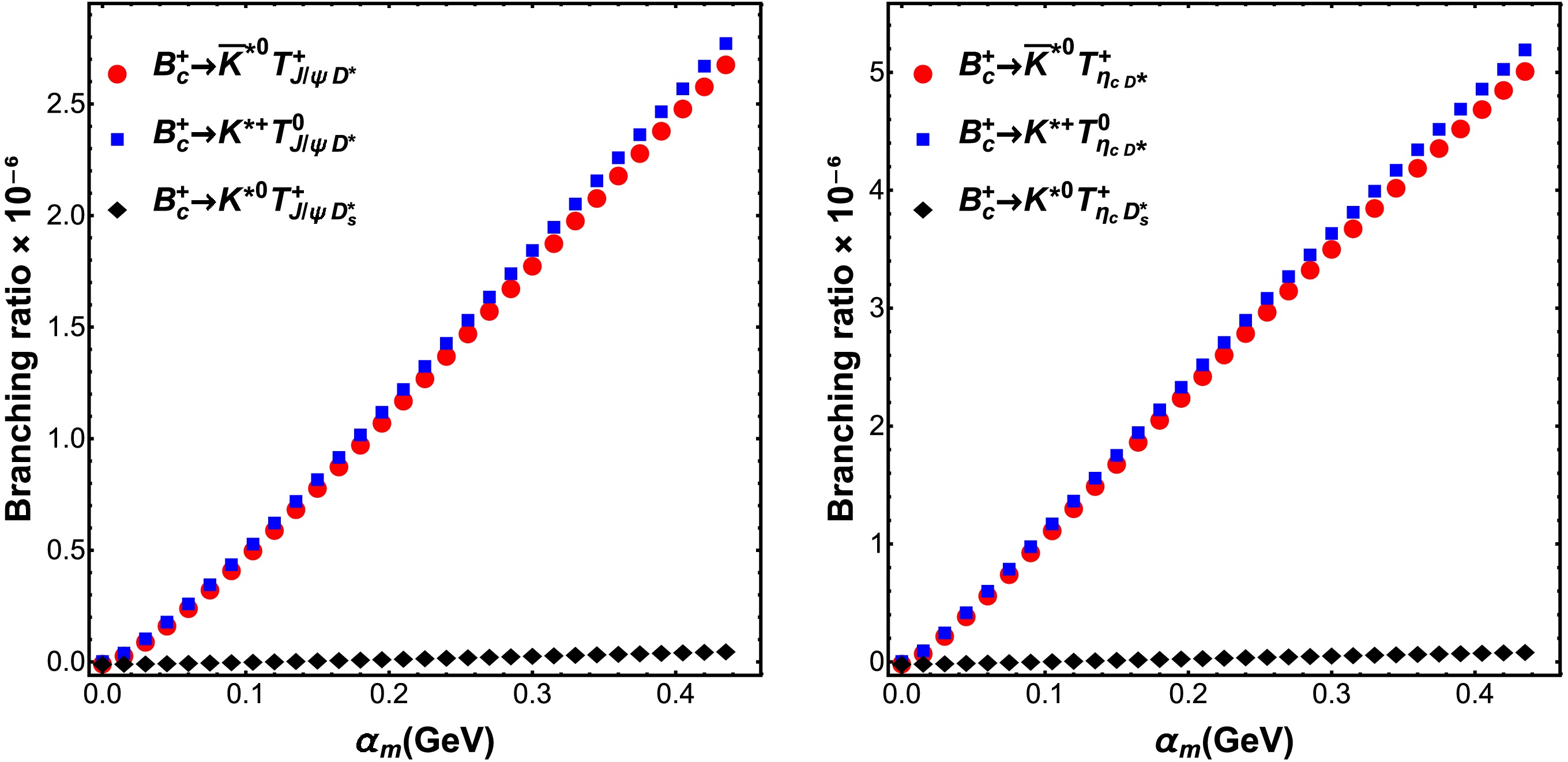
Figure 3. (color online) At the binding energy
$ \varepsilon = 5\ \text{MeV} $ , the branching ratios for$ B^+_c \to K^* T_{cc\bar c \bar q} $ vary with the scale parameter$ \alpha_m $ (GeV). The panels correspond to the$ J/\psi D^* $ molecular configuration (left) and the$ \eta_c D^* $ molecular configuration (right).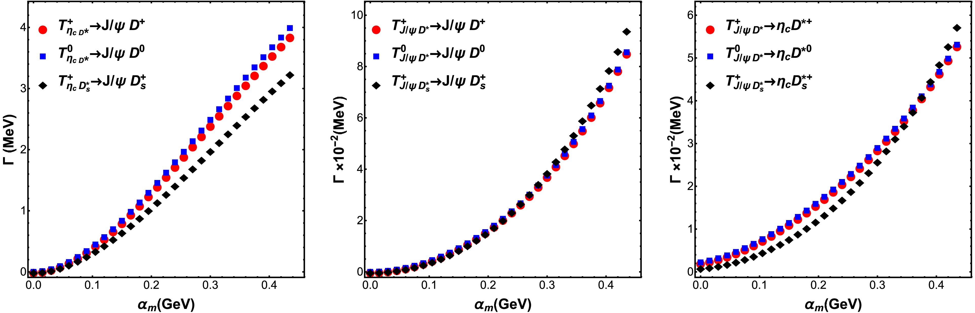
Figure 4. (color online) At the binding energy
$ \varepsilon = 5\ \text{MeV} $ , the two-body decay widths of$ T_{cc\bar c \bar q} $ vary with the scale parameter$ \alpha_m $ (GeV). The panels correspond to the decays$ T_{\eta_c D^*} \to J/\psi D $ (left),$ T_{J/\psi D^*} \to J/\psi D $ (middle), and$ T_{J/\psi D^*} \to \eta_c D^* $ (right).● In general, the production branching ratios for the
$ T_{\eta_c D^*} $ molecular configuration are larger than those for the$ T_{J/\psi D^*} $ molecule. Specifically, the branching ratios for the two Cabibbo-allowed processes$ B_c^+ \to \overline K^{*0} T_{\eta_c D^* }^{+} $ and$ B_c^+ \to K^{*+} T_{\eta_c D^*}^{0} $ can be of order$ 10^{-4} $ .$ \begin{aligned}[b]& Br(B_c^+ \to \overline K^{*0} T_{\eta_c D^*}^+) = 1.127\times10^{-4},\\& Br(B_c^+ \to K^{*+} T_{\eta_c D^*}^{0}) = 1.162\times10^{-4},\\& Br(B_c^+ \to \overline K^{*0} T_{J/\psi D^*}^+) = 8.160\times10^{-6},\\& Br(B_c^+ \to K^{*+} T_{J/\psi D^*}^{0}) = 8.400\times10^{-6}. \end{aligned} $
(23) ● We define two ratios,
$ R_1 $ and$ R_2 $ , for the production processes:$\begin{aligned}[b]& R_1 = \frac{{\Gamma(B_c^+\to K^{*+} T_{J/\psi D^*}^{0})}}{\Gamma(B_c^+\to \overline{K}^{*0} T_{J/\psi D_s^*}^+)}\approx 42,\\& R_2 = \frac{\Gamma(B_c^+\to \overline{K}^{*0} T_{\eta_c D^*}^+)}{\Gamma(B_c^+\to \overline{K}^{*0} T_{\eta_c D_s^*}^+)}\approx 50.7,\end{aligned} $
(24) These values differ from the SU(3)-symmetric prediction
$ R_{1,2} = |V_{cs}|^2/|V_{cd}|^2 \approx 19.9 $ given in Eq. (8). These results indicate that the two processes exhibit significant SU(3) flavor-symmetry breaking effects. Phase-space effects and the dynamics of loop diagrams are likely the primary mechanisms responsible for these deviations. In the loop and phase-space integrals, the propagator of the exchanged particle$ {\cal{S}}_{ex}(k_3) $ in the triangle diagram and the strong form factors$ {\cal{F}}_2(k_3^2) $ at the vertices lead to final-state dynamical effects that deviate significantly from the SU(3)-symmetry expectation, owing to differences in the masses, decay constants, and coupling constants of the D and$ D_s $ mesons.● Note that the leading-order contributions to some three-body processes arise from tree-level hadronic diagrams, such as the processes
$ T^+_{\eta_c D^*} \to D^0 \eta_c \pi^+ $ and$ T^+_{J/\psi D^*} \to D^0 J/\psi \pi^+ $ ; the calculations begin with the triangle diagrams shown in Fig. 2(b,$ b^\prime $ ).● In addition to the cutoff parameter
$ \alpha_m $ and the binding energy ϵ, the uncertainties in the production and decay processes primarily arise from the strong coupling constants associated with the$ T_{\eta_c D^*} $ and$ T_{J/\Psi D^*} $ states, as well as from the three-meson interactions. Specifically, variations in the former lead to a 12% change in the production branching fraction and an 8% change in the decay width, respectively. When a$ \pm10$ % variation in the three-meson coupling constants, arising from SU(4) flavor symmetry breaking, is further taken into account, the production branching fraction and decay width exhibit changes of 20% and 32%, respectively. Combining both sources of uncertainty, the overall production branching fraction and decay width are modified by 24% and 26%, respectively.● Summing over all possible two-body and three-body processes, we derive the total decay widths of the molecular states
$ T_{\eta_c D^*} $ and$ T_{J/\Psi D^*} $ with$ J^P = 1^+ $ for the cutoff parameter$ \alpha = 0.4 $ GeV and the binding energy$ \epsilon = 5 $ MeV.$ \Gamma(T^+_{\eta_c D^*}) = 6.8 \text{MeV},\quad \Gamma(T^+_{J/\psi D^*}) = 0.16 \text{MeV}, $
(25) Given existing studies based on different methodologies and internal structure models, we perform a direct comparison. Our results are consistent with those calculated using the Gaussian Expansion Method (GEM) [29], in which the authors predict a narrow resonance in a fully coupled-channel calculation with a total width of approximately
$ \Gamma(cc\bar c\bar q) = 3.0 $ MeV.For comparison, the compact tetraquark scheme within the constituent quark model [64] yields a relatively large decay width,
$ \Gamma(cc\bar c\bar q) = 240.8 $ MeV, with significant contributions coming from the decay modes$ J/\psi D^* $ ,$ J/\psi D $ , and$ \eta_c D^* $ . The relative decay widths are approximately$ \Gamma(J/\Psi D^*):\Gamma(\eta_c D^*):\Gamma(J/\Psi D) = 0.004:1.3:1 $ [26, 64] for the lowest$ J^P = 1^+ $ compact tetraquark states.● For completeness, we further analyze decays into final states containing light mesons, such as
$ D\rho $ and$ D^*\pi $ . These decay channels involve annihilation of the$ c\overline{c} $ component and creation of light quark pairs, and are subject to both OZI- and$ \alpha_s $ -order suppressions. In addition, they require the exchange of hard gluons and therefore suffer dynamical suppression due to the large charm-quark mass. Nevertheless, we employ the effective Lagrangian approach to compute these processes. The triangle diagrams are shown in Fig 2 ($ a^{\prime \prime} $ ,$ b^{\prime \prime} $ ,$ c^{\prime \prime} $ ). For$ T^+_{\eta_c D^*} $ and$ T^+_{J/\psi D^*} $ configurations, the decay widths with$ \epsilon = 20 $ MeV are$\begin{aligned}[b]& \Gamma(T^+_{\eta_c D^*} \to \rho^0 D^+) = 0.537\ \text{MeV},\\& \Gamma(T^+_{\eta_c D^*} \to D^{*+}\pi^0) = 0.290\ \text{MeV},\end{aligned} $
(26) $\begin{aligned}[b]& \Gamma(T_{J/\psi D^*}^+ \to \rho^0 D^+) = 0.0038\ \text{MeV},\\& \Gamma(T_{J/\psi D^*}^+ \to D^{*+}\pi^0) = 0.0038\ \text{MeV}.\end{aligned} $
(27) They are about one to two orders of magnitude smaller than the two-body decay widths listed in Table 4. Therefore, such
$ c\bar c $ annihilation decay processes do not constitute the dominant contribution. For brevity, we do not provide a detailed discussion of these processes in the present paper. -
The form factors in Eqs. (14) and (15) can be parameterized over the physical region.
$ f(q^2) = \alpha_1 +\alpha_2 q^2+\frac{\alpha_3 q^4}{m_{B_c}^2-q^2} \,, $
where the fitted parameters
$ \alpha_{1,2,3} $ are taken from reference [60]. The decay constants, coupling constants and Wilson coefficient$ a_1 $ are collected into Table 2. The coupling constants$ g_{{ T_{{ \eta_c D^*}} }} $ and$ g_{{ T_{{ J/\psi D^*}} }} $ between the molecular states$ cc\bar c\bar q $ state and their constituent can be obtained by Eq. (5). The couplings does not vary significantly with the scale parameter$ \Lambda_T $ . We take$ \Lambda_T $ from 0.8 to 1.2 GeV, the variation in the strong coupling constant is less than 6%. The three-meson strong couplings constants are derived from the SU(4) flavor symmetry analysis. It should be emphasized that incorporating${S U}(4)$ flavor symmetry breaking effects into our calculation is challenging, as this symmetry serves as the foundation of the hadronic effective Lagrangian we employ. Nevertheless, to assess how potential uncertainties in these parameters, we varied the coupling constants by$ \pm 10 $ % in the numerical analysis.$ f_{D}=0.200 $ GeV,$\quad f_{D_s}=0.241 $ GeV,$\quad f_{D^*}=0.200 $ GeV,$\quad f_{D^*_s}=0.241 $ GeV,$\quad a_{1}=1.07 $ ,$ a_2=-0.017 $ ,$\quad g_{K^*D^*D}=-7.07 $ ,$\quad g_{D^*D^*J/\psi}=2.298 $ ,$\quad g_{D^*D^*K^*}=-2.298 $ ,$ g_{D^{*+}D^0\pi^+}=16.818 $ ,$\quad g_{D^{*0}D^0\pi^0}=11.688 $ ,$\quad g_{\eta_c DD^*}=-4.271 $ ,$\quad g_{D^*D^*\eta_c}=-7.07 $ ,$ g_{J/\psi D^*D}=-7.07 $ ,$\quad g_{T_{J/\psi D^*}}=1.223^{+0.045}_{-0.024} $ ,$\quad g_{T_{\eta_c D^*}}=16.065^{+0.935}_{-0.605} $ In the schemes of molecular states
$ T_{J/\psi D^*} $ and$ T_{\eta_c D^*} $ , the production branching ratios from$ B_c $ meson are listed in Table 3, where we take cutoff parameter$ \alpha_m = 0.4 $ GeV and binding energy$ \epsilon = $ 5, 10, 20 MeV. Besides, the decay widths are obtained in Table 4, in which the results not provided are mainly forbidden by the effect of phase space. For completeness, the dependence of the production branching ratios and the two-body decay widths of the four-quark states on the cutoff parameter$ \alpha_m $ are shown in Fig. 3 and Fig. 4, respectively, with$ \alpha_m $ varying in the range of$ 100-450 $ MeV [58]. Note that the widths of three-body decays are generally small, especially for processes with only loop-diagram contributions, and they depend very weakly on$ \alpha_m $ , though a slight increasing trend is observed as$ \alpha_m $ increases.$ \eta_c D^* $ branching ratio ( $ \times 10^{-5} $ )$ J/\psi D^* $ branching ratio ( $ \times 10^{-5} $ )$ \epsilon=5 $ $ \epsilon=10 $ $ \epsilon=20 $ $ \epsilon=5 $ $ \epsilon=10 $ $ \epsilon=20 $ $B_c^+ \to \overline K^{*0} T_{\eta_c D^*}^{+} $ 4.649 $ 6.198 $ 11.272 $ B_c^+ \to \overline K^{*0} T_{J/\psi D^*}^{+} $ 0.245 $ 0.422 $ 0.816 $\quad\; \to K^{*+} T_{\eta_c D^*}^{0} $ 4.798 $ 6.393 $ 11.621 $\quad\; \to K^{*+} T_{J/\psi D^*}^{0} $ 0.253 $ 0.435 $ 0.840 $ \quad\; \to K^{*0} T_{\eta_c D_s^*}^{+} $ 0.093 $ 0.125 $ 0.229 $\quad\; \to K^{*0} T_{J/\psi D_s^*}^{+} $ 0.005 $ 0.009 $ 0.020 Table 3. The production branching ratios (
$ \times 10^{-5} $ ) for the molecular states$ cc\bar c\bar q $ with binding energies$ \epsilon=5,10,20 $ MeV.process widths $\rm /MeV$ process widths $\rm /MeV$ $ \epsilon=5 $ $ \epsilon=10 $ $ \epsilon=20 $ $ \epsilon=5 $ $ \epsilon=10 $ $ \epsilon=20 $ $ T^+_{\eta_c D^*} $ $ \to J/\psi D^+ $ 3.491 4.093 $ 4.385 $ $ T^0_{\eta_c D^*} $ $ \to J/\psi D^0 $ 3.621 4.477 $ 4.583 $ $ \to D^+ \eta_c \pi^0 $ 0.998 − − $ \to D^0 \eta_c \pi^0 $ 0.964 − − $ \to D^0 \eta_c \pi^+ $ 2.290 − − $ T^+_{\eta_c D_s^*} $ $ \to J/\psi D^+_s $ 2.293 $ 3.757 $ 3.854 $ T^+_{J/\psi D^*} $ $ \to J/\psi D^+ $ 0.070 $ 0.122 $ 0.238 $ T^0_{J/\psi D^*} $ $ \to J/\psi D^0 $ 0.070 $ 0.123 $ 0.239 $ \to \eta_c {D^*}^+ $ 0.045 $ 0.076 $ 0.141 $ \to \eta_c {D^*}^0 $ 0.045 $ 0.077 $ 0.142 $ \to D^+ J/\psi \pi^0 $ $ 0.015 $ − − $ \to D^0 J/\psi \pi^0 $ $ 0.019 $ − − $ \to D^0 J/\psi \pi^+ $ 0.025 − − $ \to D^0 \eta_c \pi^0 $ $ 1.8\times10^{-4} $ $ 3.2\times10^{-4} $ $ 6.5\times10^{-4} $ $ \to D^+ \eta_c \pi^0 $ $ 1.9\times10^{-4} $ $ 3.5\times10^{-4} $ $ 7.0\times10^{-4} $ $ T^+_{J/\psi D_s^*} $ $ \to J/\psi D^+_s $ 0.076 $ 0.136 $ 0.267 $ \to D^0 \eta_c \pi^+ $ $ 2.4\times10^{-4} $ $ 4.3\times10^{-4} $ $ 8.6\times10^{-4} $ $ \to \eta_c {D_s^*}^+ $ 0.047 $ 0.083 $ 0.163 Table 4. Partial decay widths (in units of
$\rm MeV$ ) for the two- and three-body decays of the four-quark molecular states$ T_{J/\psi D^*} $ and$ T_{\eta_c D^*} $ .
Figure 3. (color online) At the binding energy
$ \varepsilon = 5\ \text{MeV} $ , the branching ratios for$ B^+_c \to K^* T_{cc\bar c \bar q} $ vary with the scale parameter$ \alpha_m $ (GeV). The panels correspond to the$ J/\psi D^* $ molecular configuration (left) and the$ \eta_c D^* $ molecular configuration (right).
Figure 4. (color online) At the binding energy
$ \varepsilon = 5\ \text{MeV} $ , the two-body decay widths of$ T_{cc\bar c \bar q} $ vary with the scale parameter$ \alpha_m $ (GeV). The panels correspond to the decays$ T_{\eta_c D^*} \to J/\psi D $ (left),$ T_{J/\psi D^*} \to J/\psi D $ (middle), and$ T_{J/\psi D^*} \to \eta_c D^* $ (right).● In general, the production branching ratios for the
$ T_{\eta_c D^*} $ molecular configuration are larger than those for the$ T_{J/\psi D^*} $ molecule. Specifically, the branching ratios for the two Cabibbo-allowed processes$ B_c^+ \to \overline K^{*0} T_{\eta_c D^* }^{+} $ and$ B_c^+ \to K^{*+} T_{\eta_c D^*}^{0} $ can be of order$ 10^{-4} $ .$ \begin{aligned}[b]& {\rm Br}(B_c^+ \to \overline K^{*0} T_{\eta_c D^*}^+) = 1.127\times10^{-4},\\& {\rm Br}(B_c^+ \to K^{*+} T_{\eta_c D^*}^{0}) = 1.162\times10^{-4},\\& {\rm Br}(B_c^+ \to \overline K^{*0} T_{J/\psi D^*}^+) = 8.160\times10^{-6},\\& {\rm Br}(B_c^+ \to K^{*+} T_{J/\psi D^*}^{0}) = 8.400\times10^{-6}. \end{aligned} $
(23) ● We define two ratios,
$ R_1 $ and$ R_2 $ , for the production processes:$\begin{aligned}[b]& R_1 = \frac{{\Gamma(B_c^+\to K^{*+} T_{J/\psi D^*}^{0})}}{\Gamma(B_c^+\to \overline{K}^{*0} T_{J/\psi D_s^*}^+)}\approx 42,\\& R_2 = \frac{\Gamma(B_c^+\to \overline{K}^{*0} T_{\eta_c D^*}^+)}{\Gamma(B_c^+\to \overline{K}^{*0} T_{\eta_c D_s^*}^+)}\approx 50.7.\end{aligned} $
(24) These values differ from the SU(3)-symmetric prediction
$ R_{1,2} = |V_{cs}|^2/|V_{cd}|^2 \approx 19.9 $ given in Eq. (8). These results indicate that the two processes exhibit significant SU(3) flavor-symmetry breaking effects. Phase-space effects and the dynamics of loop diagrams are likely the primary mechanisms responsible for these deviations. In the loop and phase-space integrals, the propagator of the exchanged particle$ {\cal{S}}_{ex}(k_3) $ in the triangle diagram and the strong form factors$ {\cal{F}}_2(k_3^2) $ at the vertices lead to final-state dynamical effects that deviate significantly from the SU(3)-symmetry expectation, owing to differences in the masses, decay constants, and coupling constants of the D and$ D_s $ mesons.● Note that the leading-order contributions to some three-body processes arise from tree-level hadronic diagrams, such as the processes
$ T^+_{\eta_c D^*} \to D^0 \eta_c \pi^+ $ and$ T^+_{J/\psi D^*} \to D^0 J/\psi \pi^+ $ ; the calculations begin with the triangle diagrams shown in Fig. 2(b,$ b^\prime $ ).● In addition to the cutoff parameter
$ \alpha_m $ and the binding energy ϵ, the uncertainties in the production and decay processes primarily arise from the strong coupling constants associated with the$ T_{\eta_c D^*} $ and$ T_{J/\psi D^*} $ states, as well as from the three-meson interactions. Specifically, variations in the former lead to a 12% change in the production branching fraction and an 8% change in the decay width, respectively. When a$ \pm10$ % variation in the three-meson coupling constants, arising from SU(4) flavor symmetry breaking, is further taken into account, the production branching fraction and decay width exhibit changes of 20% and 32%, respectively. Combining both sources of uncertainty, the overall production branching fraction and decay width are modified by 24% and 26%, respectively.● Summing over all possible two-body and three-body processes, we derive the total decay widths of the molecular states
$ T_{\eta_c D^*} $ and$ T_{J/\psi D^*} $ with$ J^P = 1^+ $ for the cutoff parameter$ \alpha = 0.4 $ GeV and the binding energy$ \epsilon = 5 $ MeV.$ \Gamma(T^+_{\eta_c D^*}) = 6.8 \;\text{MeV},\quad \Gamma(T^+_{J/\psi D^*}) = 0.16 \;\text{MeV}. $
(25) Given existing studies based on different methodologies and internal structure models, we perform a direct comparison. Our results are consistent with those calculated using the Gaussian Expansion Method (GEM) [28], in which the authors predict a narrow resonance in a fully coupled-channel calculation with a total width of approximately
$ \Gamma(cc\bar c\bar q) = 3.0 $ MeV.For comparison, the compact tetraquark scheme within the constituent quark model [63] yields a relatively large decay width,
$ \Gamma(cc\bar c\bar q) = 240.8 $ MeV, with significant contributions coming from the decay modes$ J/\psi D^* $ ,$ J/\psi D $ , and$ \eta_c D^* $ . The relative decay widths are approximately$ \Gamma(J/\psi D^*):\Gamma(\eta_c D^*):\Gamma(J/\psi D) = 0.004:1.3:1 $ [25, 63] for the lowest$ J^P = 1^+ $ compact tetraquark states.● For completeness, we further analyze decays into final states containing light mesons, such as
$ D\rho $ and$ D^*\pi $ . These decay channels involve annihilation of the$ c\overline{c} $ component and creation of light quark pairs, and are subject to both OZI- and$ \alpha_s $ -order suppressions. In addition, they require the exchange of hard gluons and therefore suffer dynamical suppression due to the large charm-quark mass. Nevertheless, we employ the effective Lagrangian approach to compute these processes. The triangle diagrams are shown in Fig 2 ($ a^{\prime \prime} $ ,$ b^{\prime \prime} $ ,$ c^{\prime \prime} $ ). For$ T^+_{\eta_c D^*} $ and$ T^+_{J/\psi D^*} $ configurations, the decay widths with$ \epsilon = 20 $ MeV are$\begin{aligned}[b]& \Gamma(T^+_{\eta_c D^*} \to \rho^0 D^+) = 0.537\ \text{MeV},\\& \Gamma(T^+_{\eta_c D^*} \to D^{*+}\pi^0) = 0.290\ \text{MeV},\end{aligned} $
(26) $\begin{aligned}[b]& \Gamma(T_{J/\psi D^*}^+ \to \rho^0 D^+) = 0.0038\ \text{MeV},\\& \Gamma(T_{J/\psi D^*}^+ \to D^{*+}\pi^0) = 0.0038\ \text{MeV}.\end{aligned} $
(27) They are about one to two orders of magnitude smaller than the two-body decay widths listed in Table 4. Therefore, such
$ c\bar c $ annihilation decay processes do not constitute the dominant contribution. For brevity, we do not provide a detailed discussion of these processes in the present paper. -
In this work, we investigate the production of the molecular states
$ T_{J/\psi D^*} $ and$ T_{\eta_c D^*} $ in$ B_c $ meson decays, as well as their two-body and three-body strong decays. Starting from an SU(3)-symmetric phenomenological analysis, we identify several golden channels for the production and decay of these four-quark molecular states. Using the effective Lagrangian approach, we compute the decay widths and production branching ratios. We find that the production branching ratios increase with both the cutoff parameter$ \alpha_m $ and the binding energy ϵ. For the$ T_{\eta_c D^*} $ configuration, the branching ratios can reach the order of$ 10^{-4} $ . Furthermore, the predicted strong-decay widths of both$ T_{\eta_c D^*} $ and$ T_{J/\psi D^*} $ are modest, of order MeV. -
We thank Prof. LiSheng Geng for the meaningful discussion remarks and useful comments.
-
We thank Prof. LiSheng Geng for the meaningful discussion remarks and useful comments.
-
We thank Prof. LiSheng Geng for the meaningful discussion remarks and useful comments.
-
We thank Prof. LiSheng Geng for the meaningful discussion remarks and useful comments.
-
The coupling constants
$ {g^2_{T_{{ {\eta_c D^*} }}}} $ and$ {g^2_{T_{{ {J/\psi D^*} }}}} $ can be deduced as follows:$ \begin{aligned}[b] \dfrac{1}{{g^2_{T_{{{\eta_c D^*}}}}} } =\;& 3 \int_{0}^{1}{\rm d}\alpha\int_{0}^{\infty}{\rm d}\beta\dfrac{\beta}{16\pi^{2}} \dfrac{\partial^2}{\partial p^2} \Big( \dfrac{-3\Phi^2(\Delta)}{(1+\beta)^2}+\dfrac{\Lambda_T^{2}\Phi^2(\Delta)}{2{m^2_{{D^*}}}}\Big(\dfrac{2}{(-1-\beta)^3}+\dfrac{1}{(1+\beta)^4}\times\dfrac{p^{2}}{2\Lambda_T^{2}} \times(2(1-\alpha)\beta-\dfrac{-2{m_{{D^*}}}}{{m_{{\eta_c}}}+{m_{{D^*}}}})^2p^2\Big) \\ &-\dfrac{\Lambda_T^4\Phi^2(\Delta)}{4m_{T_{{\eta_c D^*}}}^2{m_{{D^*}}}^2}\Big(\dfrac{1}{(1+\beta)^4}\dfrac{p^4}{4\Lambda_T^4}\times(4(\alpha-1)\beta +2\dfrac{-2m_{{D^*}}}{m_{\eta_c}+m_{{D^*}}})^2+\dfrac{1}{(-1-\beta)^3}\times\dfrac{p^2}{\Lambda_T^2}\Big)\Big), \\ \dfrac{1}{g^2_{T_{{{J/\psi D^*}}}}} =\;& 3 \int_{0}^{1}{\rm d}\alpha\int_{0}^{\infty}{\rm d}\beta\dfrac{\beta}{16\pi^{2}}\dfrac{\partial^2}{\partial p^2}\Big( \dfrac{-\Lambda_T^4\Delta_5}{2{m^2_{{J/\psi}}}}-\dfrac{6p^2}{(-1-\beta)^2} \Phi^2(\Delta)+\dfrac{\Lambda_T^2p^2\Delta_1 }{m^2_{{J/\psi}}} +\dfrac{p^2}{{m^2_{{{{ D^*}}}}}{m^2_{{{{J/\psi}}}}}}\dfrac{\Lambda_T^4}{4} (\Delta_3-2\Delta_4+\Delta_5)\\ &+\dfrac{1}{{m^2_{{{{ D^*}}}}}{m^2_{{{{J/\psi}}}}}}(\dfrac{\Lambda_T^6\Delta_6-2\Lambda_T^6 \Delta_7+2{\Lambda_T^4}}{8})+(\dfrac{\Lambda_T^2}{2}\Delta_1-\Lambda_T^2\Delta_2 +p^2)\dfrac{2p^2}{{m^2_{{D_{(s)}^*}}}}-\dfrac{p^4 \Delta_5}{{m^2_{{{{ D^*}}}}}{m^2_{{{{J/\psi}}}}}}(\dfrac{\Lambda_T^4 \Delta_3-2{\Lambda_T^4 \Delta_4}+2{\Lambda_T^2\Delta_1p^2}}{4})\\ &-\dfrac{2}{m^2_{{J/\psi}}}(\dfrac{\Lambda_T^4 \Delta_5}{4}+p^4 -\Lambda_T^2\Delta_2p^2)-\dfrac{1}{{m^2_{{{{ D^*}}}}}{m^2_{{{{J/\psi}}}}}} (\dfrac{\Lambda_T^6 \Delta_6}{4}-\dfrac{\Lambda_T^4 \Delta_4p^2}{2}+\dfrac{\Lambda_T^4 \Delta_5 p^2}{2}-\dfrac{\Lambda_T^6 \Delta_7}{4}) \\ &+\dfrac{1}{{m^2_{{{{ D^*}}}}}{m^2_{{{{J/\psi}}}}}} (\dfrac{\Lambda_T^6 \Delta_6}{8} - \dfrac{\Lambda_T^4 \Delta_4p^2}{2}+\dfrac{\Lambda_T^2 \Delta_1p^4}{2})\Big), \end{aligned} $
(A1) where
$ \Delta = \dfrac{-m_{D^*}}{m_{\eta_c}+m_{D^*}}p^2+\alpha\beta m_{D^*}^2+(1-\alpha)\beta( p^2- m_{\eta_c}^2)-\dfrac{1}{4}\dfrac{(2(1-\alpha)\beta-\dfrac{2m_{D^*}}{m_{\eta_c}+m_{D^*}})^2}{-1-\beta}p^2 $ . Throughout this work, we take$ \Lambda_T = 1 $ GeV.$ \begin{aligned}[b] \Delta^{\prime} =\;& -\dfrac{m^2_{{D^*}}}{m_{{J/\psi}}+m_{{D^*}}}p^2+\alpha\beta m_{{D^*}}^2-(1-\alpha)\beta p^2+(1-\alpha)\beta m_{{J/\psi}}^2+\dfrac{\Big(2(1-\alpha)\beta-\dfrac{-2m_{{D^*}}}{m_{{J/\psi}}+m_{{D^*}}}\Big)^2}{4(1+\beta)}p^2,\\ \Delta_1 =\;& \dfrac{\left(2 \times(1-\alpha) \beta+\dfrac{2 m_{{D^*}}}{m_{{J/\psi}}+m_{{D^*}}}\right)^2 \Phi^2({\Delta^{\prime}})}{2(-\beta-1)^4 \Lambda_T^2}, \quad\Delta_2 = \dfrac{\left(-4 \times(1-\alpha) \beta-\dfrac{4 m_{{D^*}}}{m_{{J/\psi}}+m_{{D^*}}}\right) \Phi^2(\Delta^{\prime})}{2(-\beta-1)^3 \Lambda_T^2}, \end{aligned} $
$ \begin{aligned}[b] \Delta_3 =\;& \Phi^2(\Delta^{\prime})\Big(\dfrac{3(2(1-\alpha)\beta+\dfrac{2m_{{D^*}}}{m_{{J/\psi}}+m_{{D^*}}})^2 }{(-\beta-1)^5\Lambda_T^2}+\dfrac{p^2(2(1-\alpha)\beta+\dfrac{2m_{{D^*}}}{m_{{J/\psi}}+m_{{D^*}}})^4 }{2(-\beta-1)^6\Lambda_T^4}\Big),\\ \Delta_4 =\;& \Phi^2(\Delta^{\prime})\Big(\dfrac{3(4 \beta(\alpha-1) -\dfrac{4 m_{{D^*}}}{m_{{J/\psi}}+m_{{D^*}}}) }{2(\beta+1)^4 \Lambda_T^2}+\dfrac{p^2(4 (\alpha-1) \beta-\dfrac{4 m_{{D^*}}}{m_{{J/\psi}}+m_{{D^*}}})(2 \beta(1-\alpha)+\dfrac{2 m_{{D^*}}}{m_{{J/\psi}}+m_{{D^*}}})^2 }{2(-\beta-1)^5 \Lambda_T^4}\Big),\\ \Delta_5 =\;& \Phi^2(\Delta^{\prime})\Big(\dfrac{-4 \times(1-\alpha) \beta-\dfrac{4 m_{{D^*}}}{m_{{J/\psi}}+m_{{D^*}}} }{(-\beta-1)^3 \Lambda_T^2}+\dfrac{p^2(-4 \times(1-\alpha) \beta-\dfrac{4 m_{{D^*}}}{m_{{J/\psi}}+m_{{D^*}}}) }{2(\beta+1)^4 \Lambda_T^4}\Big),\\ \Delta_6 =\;& \Phi^2(\Delta^{\prime})\Big(\dfrac{3}{(-\beta-1)^4 \Lambda_T^2}+\dfrac{2 p^2(-4 \times(1-\alpha) \beta-\dfrac{4 m_{V_1}}{m_{{J/\psi}}+m_{V_1}})^2 }{(-\beta-1)^5 \Lambda_T^4} + \dfrac{p^2(2 \times(1-\alpha) \beta+\dfrac{2m_{V_1}}{m_{{J/\psi}}+m_{V_1}})^2 }{(-\beta-1)^5 \Lambda_T^4}, \\&+\dfrac{3 p^4(4 \times(\alpha-1) \beta-\dfrac{4 m_{{D^*}}}{m_{{J/\psi}}+m_{{D^*}}})^2(2 \times(1-\alpha) \beta+\dfrac{2 m_{{D^*}}}{m_{{J/\psi}}+m_{{D^*}}})^2 }{8(\beta+1)^6 \Lambda_T^6}\Big ),\\ \Delta_7 =\;& \Phi^2(\Delta^{\prime})\Big( \dfrac{12p^2\alpha \beta-12p^2 \beta-12p^2 \dfrac{m_{{D^*}}}{m_{{J/\psi}}+m_{{D^*}}}}{(\beta+1)^4 \Lambda_T^4}+\dfrac{3p^4((\alpha-1) \beta-\dfrac{ m_{{D^*}}}{m_{{J/\psi}}+m_{{D^*}}})^3 }{2(-\beta-1)^5\Lambda_T^6}\Big). \end{aligned} $
(A2) The full set of production and decay channels for four-quark molecular states is collected in Table A1 and Table A2. In addition, the complete relations among different production processes are listed.
$ \begin{aligned}[b]& \Gamma(B_c^+\to \rho^0 T_{J/\psi D^*}^+) = \frac{1}{2}\Gamma(B_c^+\to \rho^+ T_{J/\psi D^*}^{0}) = \frac{1}{2}\Gamma(B_c^+\to \overline{K}^{*0} T_{J/\psi D_s^*}^+), \\& \Gamma(B_c^+\to K^{*+} T_{J/\psi D^*}^{0}) = \Gamma(B_c^+\to K^{*0} T_{J/\psi D^*}^+) = \Gamma(B_c^+\to \phi T_{J/\psi D_s^*}^+),\\& \Gamma(B_c^+\to \rho^0 T_{\eta_c D^*}^+) = \frac{1}{2}\Gamma(B_c^+\to \rho^+ T_{\eta_c D^*}^{0}) = \frac{1}{2}\Gamma(B_c^+\to \overline{K}^{*0} T_{\eta_c D_s^*}^+),\\& \Gamma(B_c^+\to K^{*+} T_{\eta_c D^*}^{0}) = \Gamma(B_c^+\to K^{*0} T_{\eta_c D^*}^+) = \Gamma(B_c^+\to \phi T_{\eta_c D_s^*}^+). \end{aligned} $
(A3) The relations among different decay channels are given by:
$ \begin{aligned}[b]& \Gamma(T_{J/\psi D^*}^{0}\to \eta_c D^{*0}) = \Gamma(T_{J/\psi D^*}^+\to \eta_c D^{*+}) = \Gamma(T^+_{J/\psi D_s^*}\to \eta_c D^{*+}_s),\,\,\,\\& \Gamma(T_{J/\psi D^*}^{0}\to J/\psi D^0) = \Gamma(T_{J/\psi D^*}^+\to J/\psi D^+) = \Gamma(T_{J/\psi D_s^*}^+\to J/\psi D^+_s),\,\,\,\\& \Gamma(T^0_{\eta_c D^{*0}}\to J/\psi D^0) = \Gamma(T^+_{\eta_c D^{*0}}\to J/\psi D^+) = \Gamma(T_{\eta_c D_s^*}^+\to \eta_c D^{*+}_s),\,\,\, \\& \Gamma(T_{J/\psi D^*}^{0}\to D^+ J/\psi \pi^- ) = \Gamma(T_{J/\psi D^*}^{0}\to D^+_s J/\psi K^- ) = \Gamma(T_{J/\psi D^*}^+\to D^0 J/\psi \pi^+ )\\& = \Gamma(T_{J/\psi D^*}^+\to D^+_s J/\psi \overline K^0) = \Gamma(T_{J/\psi D_s^*}^+\to D^0 J/\psi K^+ ) = \Gamma(T_{J/\psi D_s^*}^+\to D^+ J/\psi K^0) \\& = 2\Gamma(T_{J/\psi D^*}^{0}\to D^0 J/\psi \pi^0 ) = 2\Gamma(T_{J/\psi D^*}^+\to D^+ J/\psi \pi^0) = 6\Gamma(T_{J/\psi D^*}^{0}\to D^0 J/\psi \eta_q )\\& = 6\Gamma(T_{J/\psi D^*}^+\to D^+ J/\psi \eta_q ) = \frac{3}{2}\Gamma(T_{J/\psi D_s^*}^+\to D^+_s J/\psi \eta_q ),\,\,\,\Gamma(T_{J/\psi D^*}^{0}\to D^+ \eta_c \pi^- )\\ &= \Gamma(T_{J/\psi D^*}^{0}\to D^+_s \eta_c K^- ) = \Gamma(T_{J/\psi D^*}^+\to D^0 \eta_c \pi^+ ) = \Gamma(T_{J/\psi D^*}^+\to D^+_s \eta_c \overline K^0) \\& = \Gamma(T_{J/\psi D_s^*}^+\to D^0 \eta_c K^+ ) = \Gamma(T_{J/\psi D_s^*}^+\to D^+ \eta_c K^0) = 2\Gamma(T_{J/\psi D^*}^{0}\to D^0 \eta_c \pi^0 )\\& = 2\Gamma(T_{J/\psi D^*}^+\to D^+ \eta_c \pi^0) = 6\Gamma(T_{J/\psi D^*}^{0}\to D^0 \eta_c \eta_q ) = 6\Gamma(T_{J/\psi D^*}^+\to D^+ \eta_c \eta_q )\\ &= \frac{3}{2}\Gamma(T_{J/\psi D_s^*}^+\to D^+_s \eta_c \eta_q ),\,\,\,\Gamma(T_{J/\psi D^*}^{0}\to D^+ \eta_c \pi^- ) = \Gamma(T_{J/\psi D^*}^{0}\to D^+_s \eta_c K^- )\\& = \Gamma(T_{J/\psi D^*}^+\to D^0 \eta_c \pi^+ ) = \Gamma(T_{J/\psi D^*}^+\to D^+_s \eta_c \overline K^0) = \Gamma(T_{J/\psi D_s^*}^+\to D^0 \eta_c K^+ )\\& = \Gamma(T_{J/\psi D_s^*}^+\to D^+ \eta_c K^0) = 2\Gamma(T_{J/\psi D^*}^{0}\to D^0 \eta_c \pi^0 ) = 2\Gamma(T_{J/\psi D^*}^+\to D^+ \eta_c \pi^0)\\& = 6\Gamma(T_{J/\psi D^*}^{0}\to D^0 \eta_c \eta_q ) = 6\Gamma(T_{J/\psi D^*}^+\to D^+ \eta_c \eta_q ) = \frac{3}{2}\Gamma(T_{J/\psi D_s^*}^+\to D^+_s \eta_c \eta_q ). \end{aligned} $
(A4) -
The coupling constants
$ {g^2_{T_{{ {\eta_c D^*} }}}} $ and$ {g^2_{T_{{ {J/\psi D^*} }}}} $ can be deduced as follows:$ \begin{aligned}[b] \dfrac{1}{{g^2_{T_{{{\eta_c D^*}}}}} } =\;& 3 \int_{0}^{1}d\alpha\int_{0}^{\infty}d\beta\dfrac{\beta}{16\pi^{2}} \dfrac{\partial^2}{\partial p^2} \Big( \dfrac{-3\Phi^2(\Delta)}{(1+\beta)^2}+\dfrac{\Lambda_T^{2}\Phi^2(\Delta)}{2{m^2_{{D^*}}}}\Big(\dfrac{2}{(-1-\beta)^3}+\dfrac{1}{(1+\beta)^4}\times\dfrac{p^{2}}{2\Lambda_T^{2}} \times(2(1-\alpha)\beta-\dfrac{-2{m_{{D^*}}}}{{m_{{\eta_c}}}+{m_{{D^*}}}})^2p^2\Big) \\ &-\dfrac{\Lambda_T^4\Phi^2(\Delta)}{4m_{T_{{\eta_c D^*}}}^2{m_{{D^*}}}^2}\Big(\dfrac{1}{(1+\beta)^4}\dfrac{p^4}{4\Lambda_T^4}\times(4(\alpha-1)\beta +2\dfrac{-2m_{{D^*}}}{m_{\eta_c}+m_{{D^*}}})^2+\dfrac{1}{(-1-\beta)^3}\times\dfrac{p^2}{\Lambda_T^2}\Big)\Big), \\ \dfrac{1}{g^2_{T_{{{J/\psi D^*}}}}} =\;& 3 \int_{0}^{1}d\alpha\int_{0}^{\infty}d\beta\dfrac{\beta}{16\pi^{2}}\dfrac{\partial^2}{\partial p^2}\Big( \dfrac{-\Lambda_T^4\Delta_5}{2{m^2_{{J/\psi}}}}-\dfrac{6p^2}{(-1-\beta)^2} \Phi^2(\Delta)+\dfrac{\Lambda_T^2p^2\Delta_1 }{m^2_{{J/\psi}}} +\dfrac{p^2}{{m^2_{{{{ D^*}}}}}{m^2_{{{{J/\psi}}}}}}\dfrac{\Lambda_T^4}{4} (\Delta_3-2\Delta_4+\Delta_5)\\ &+\dfrac{1}{{m^2_{{{{ D^*}}}}}{m^2_{{{{J/\psi}}}}}}(\dfrac{\Lambda_T^6\Delta_6-2\Lambda_T^6 \Delta_7+2{\Lambda_T^4}}{8})+(\dfrac{\Lambda_T^2}{2}\Delta_1-\Lambda_T^2\Delta_2 +p^2)\dfrac{2p^2}{{m^2_{{D_{(s)}^*}}}}-\dfrac{p^4 \Delta_5}{{m^2_{{{{ D^*}}}}}{m^2_{{{{J/\psi}}}}}}(\dfrac{\Lambda_T^4 \Delta_3-2{\Lambda_T^4 \Delta_4}+2{\Lambda_T^2\Delta_1p^2}}{4})\\ &-\dfrac{2}{m^2_{{J/\psi}}}(\dfrac{\Lambda_T^4 \Delta_5}{4}+p^4 -\Lambda_T^2\Delta_2p^2)-\dfrac{1}{{m^2_{{{{ D^*}}}}}{m^2_{{{{J/\psi}}}}}} (\dfrac{\Lambda_T^6 \Delta_6}{4}-\dfrac{\Lambda_T^4 \Delta_4p^2}{2}+\dfrac{\Lambda_T^4 \Delta_5 p^2}{2}-\dfrac{\Lambda_T^6 \Delta_7}{4}) \\ &+\dfrac{1}{{m^2_{{{{ D^*}}}}}{m^2_{{{{J/\psi}}}}}} (\dfrac{\Lambda_T^6 \Delta_6}{8} - \dfrac{\Lambda_T^4 \Delta_4p^2}{2}+\dfrac{\Lambda_T^2 \Delta_1p^4}{2})\Big), \end{aligned} $
(A1) where
$ \Delta = \dfrac{-m_{D^*}}{m_{\eta_c}+m_{D^*}}p^2+\alpha\beta m_{D^*}^2+(1-\alpha)\beta( p^2- m_{\eta_c}^2)-\dfrac{1}{4}\dfrac{(2(1-\alpha)\beta-\dfrac{2m_{D^*}}{m_{\eta_c}+m_{D^*}})^2}{-1-\beta}p^2 $ . Throughout this work, we take$ \Lambda_T = 1 $ GeV.$ \begin{aligned}[b] \Delta^{\prime} =\;& -\dfrac{m^2_{{D^*}}}{m_{{J/\psi}}+m_{{D^*}}}p^2+\alpha\beta m_{{D^*}}^2-(1-\alpha)\beta p^2+(1-\alpha)\beta m_{{J/\psi}}^2+\dfrac{\Big(2(1-\alpha)\beta-\dfrac{-2m_{{D^*}}}{m_{{J/\psi}}+m_{{D^*}}}\Big)^2}{4(1+\beta)}p^2,\\ \Delta_1 =\;& \dfrac{\left(2 \times(1-\alpha) \beta+\dfrac{2 m_{{D^*}}}{m_{{J/\psi}}+m_{{D^*}}}\right)^2 \Phi^2({\Delta^{\prime}})}{2(-\beta-1)^4 \Lambda_T^2}, \quad\Delta_2 = \dfrac{\left(-4 \times(1-\alpha) \beta-\dfrac{4 m_{{D^*}}}{m_{{J/\psi}}+m_{{D^*}}}\right) \Phi^2(\Delta^{\prime})}{2(-\beta-1)^3 \Lambda_T^2}, \end{aligned} $
$ \begin{aligned}[b] \Delta_3 =\;& \Phi^2(\Delta^{\prime})\Big(\dfrac{3(2(1-\alpha)\beta+\dfrac{2m_{{D^*}}}{m_{{J/\psi}}+m_{{D^*}}})^2 }{(-\beta-1)^5\Lambda_T^2}+\dfrac{p^2(2(1-\alpha)\beta+\dfrac{2m_{{D^*}}}{m_{{J/\psi}}+m_{{D^*}}})^4 }{2(-\beta-1)^6\Lambda_T^4}\Big),\\ \Delta_4 =\;& \Phi^2(\Delta^{\prime})\Big(\dfrac{3(4 \beta(\alpha-1) -\dfrac{4 m_{{D^*}}}{m_{{J/\psi}}+m_{{D^*}}}) }{2(\beta+1)^4 \Lambda_T^2}+\dfrac{p^2(4 (\alpha-1) \beta-\dfrac{4 m_{{D^*}}}{m_{{J/\psi}}+m_{{D^*}}})(2 \beta(1-\alpha)+\dfrac{2 m_{{D^*}}}{m_{{J/\psi}}+m_{{D^*}}})^2 }{2(-\beta-1)^5 \Lambda_T^4}\Big),\\ \Delta_5 =\;& \Phi^2(\Delta^{\prime})\Big(\dfrac{(-4 \times(1-\alpha) \beta-\dfrac{4 m_{{D^*}}}{m_{{J/\psi}}+m_{{D^*}}}) }{(-\beta-1)^3 \Lambda_T^2}+\dfrac{p^2(-4 \times(1-\alpha) \beta-\dfrac{4 m_{{D^*}}}{m_{{J/\psi}}+m_{{D^*}}}) }{2(\beta+1)^4 \Lambda_T^4}\Big),\\ \Delta_6 =\;& \Phi^2(\Delta^{\prime})\Big(\dfrac{3}{(-\beta-1)^4 \Lambda_T^2}+\dfrac{2 p^2(-4 \times(1-\alpha) \beta-\dfrac{4 m_{V_1}}{m_{{J/\psi}}+m_{V_1}})^2 }{(-\beta-1)^5 \Lambda_T^4} + \dfrac{p^2(2 \times(1-\alpha) \beta+\dfrac{2m_{V_1}}{m_{{J/\psi}}+m_{V_1}})^2 }{(-\beta-1)^5 \Lambda_T^4}, \\&+\dfrac{3 p^4(4 \times(\alpha-1) \beta-\dfrac{4 m_{{D^*}}}{m_{{J/\psi}}+m_{{D^*}}})^2(2 \times(1-\alpha) \beta+\dfrac{2 m_{{D^*}}}{m_{{J/\psi}}+m_{{D^*}}})^2 }{8(\beta+1)^6 \Lambda_T^6}\Big ),\\ \Delta_7 =\;& \Phi^2(\Delta^{\prime})\Big( \dfrac{12p^2\alpha \beta-12p^2 \beta-12p^2 \dfrac{m_{{D^*}}}{m_{{J/\psi}}+m_{{D^*}}})}{(\beta+1)^4 \Lambda_T^4}+\dfrac{3p^4((\alpha-1) \beta-\dfrac{ m_{{D^*}}}{m_{{J/\psi}}+m_{{D^*}}})^3 }{2(-\beta-1)^5\Lambda_T^6}\Big). \end{aligned} $
(A2) The full set of production and decay channels for four-quark molecular states is collected in Table A1 and Table A2. In addition, the complete relations among different production processes are listed.
$ \begin{aligned}[b]& \Gamma(B_c^+\to \rho^0 T_{J/\psi D^*}^+) = \frac{1}{2}\Gamma(B_c^+\to \rho^+ T_{J/\psi D^*}^{0}) = \frac{1}{2}\Gamma(B_c^+\to \overline{K}^{*0} T_{J/\psi D_s^*}^+), \\& \Gamma(B_c^+\to K^{*+} T_{J/\psi D^*}^{0}) = \Gamma(B_c^+\to K^{*0} T_{J/\psi D^*}^+) = \Gamma(B_c^+\to \phi T_{J/\psi D_s^*}^+),\\& \Gamma(B_c^+\to \rho^0 T_{\eta_c D^*}^+) = \frac{1}{2}\Gamma(B_c^+\to \rho^+ T_{\eta_c D^*}^{0}) = \frac{1}{2}\Gamma(B_c^+\to \overline{K}^{*0} T_{\eta_c D_s^*}^+),\\& \Gamma(B_c^+\to K^{*+} T_{\eta_c D^*}^{0}) = \Gamma(B_c^+\to K^{*0} T_{\eta_c D^*}^+) = \Gamma(B_c^+\to \phi T_{\eta_c D_s^*}^+). \end{aligned} $
(A3) The relations among different decay channels are given by:
$ \begin{aligned}[b]& \Gamma(T_{J/\psi D^*}^{0}\to \eta_c D^{*0}) = \Gamma(T_{J/\psi D^*}^+\to \eta_c D^{*+}) = \Gamma(T^+_{J/\psi D_s^*}\to \eta_c D^{*+}_s),\,\,\,\\& \Gamma(T_{J/\psi D^*}^{0}\to J/\psi D^0) = \Gamma(T_{J/\psi D^*}^+\to J/\psi D^+) = \Gamma(T_{J/\psi D_s^*}^+\to J/\psi D^+_s),\,\,\,\\& \Gamma(T^0_{\eta_c D^{*0}}\to J/\psi D^0) = \Gamma(T^+_{\eta_c D^{*0}}\to J/\psi D^+) = \Gamma(T_{\eta_c D_s^*}^+\to \eta_c D^{*+}_s),\,\,\, \\& \Gamma(T_{J/\psi D^*}^{0}\to D^+ J/\psi \pi^- ) = \Gamma(T_{J/\psi D^*}^{0}\to D^+_s J/\psi K^- ) = \Gamma(T_{J/\psi D^*}^+\to D^0 J/\psi \pi^+ )\\& = \Gamma(T_{J/\psi D^*}^+\to D^+_s J/\psi \overline K^0) = \Gamma(T_{J/\psi D_s^*}^+\to D^0 J/\psi K^+ ) = \Gamma(T_{J/\psi D_s^*}^+\to D^+ J/\psi K^0) \\& = 2\Gamma(T_{J/\psi D^*}^{0}\to D^0 J/\psi \pi^0 ) = 2\Gamma(T_{J/\psi D^*}^+\to D^+ J/\psi \pi^0) = 6\Gamma(T_{J/\psi D^*}^{0}\to D^0 J/\psi \eta_q )\\& = 6\Gamma(T_{J/\psi D^*}^+\to D^+ J/\psi \eta_q ) = \frac{3}{2}\Gamma(T_{J/\psi D_s^*}^+\to D^+_s J/\psi \eta_q ),\,\,\,\Gamma(T_{J/\psi D^*}^{0}\to D^+ \eta_c \pi^- )\\ &= \Gamma(T_{J/\psi D^*}^{0}\to D^+_s \eta_c K^- ) = \Gamma(T_{J/\psi D^*}^+\to D^0 \eta_c \pi^+ ) = \Gamma(T_{J/\psi D^*}^+\to D^+_s \eta_c \overline K^0) \\& = \Gamma(T_{J/\psi D_s^*}^+\to D^0 \eta_c K^+ ) = \Gamma(T_{J/\psi D_s^*}^+\to D^+ \eta_c K^0) = 2\Gamma(T_{J/\psi D^*}^{0}\to D^0 \eta_c \pi^0 )\\& = 2\Gamma(T_{J/\psi D^*}^+\to D^+ \eta_c \pi^0) = 6\Gamma(T_{J/\psi D^*}^{0}\to D^0 \eta_c \eta_q ) = 6\Gamma(T_{J/\psi D^*}^+\to D^+ \eta_c \eta_q )\\ &= \frac{3}{2}\Gamma(T_{J/\psi D_s^*}^+\to D^+_s \eta_c \eta_q ),\,\,\,\Gamma(T_{J/\psi D^*}^{0}\to D^+ \eta_c \pi^- ) = \Gamma(T_{J/\psi D^*}^{0}\to D^+_s \eta_c K^- )\\& = \Gamma(T_{J/\psi D^*}^+\to D^0 \eta_c \pi^+ ) = \Gamma(T_{J/\psi D^*}^+\to D^+_s \eta_c \overline K^0) = \Gamma(T_{J/\psi D_s^*}^+\to D^0 \eta_c K^+ )\\& = \Gamma(T_{J/\psi D_s^*}^+\to D^+ \eta_c K^0) = 2\Gamma(T_{J/\psi D^*}^{0}\to D^0 \eta_c \pi^0 ) = 2\Gamma(T_{J/\psi D^*}^+\to D^+ \eta_c \pi^0)\\& = 6\Gamma(T_{J/\psi D^*}^{0}\to D^0 \eta_c \eta_q ) = 6\Gamma(T_{J/\psi D^*}^+\to D^+ \eta_c \eta_q ) = \frac{3}{2}\Gamma(T_{J/\psi D_s^*}^+\to D^+_s \eta_c \eta_q ). \end{aligned} $
(A4) -
The coupling constants
$ {g^2_{T_{{ {\eta_c D^*} }}}} $ and$ {g^2_{T_{{ {J/\psi D^*} }}}} $ can be deduced as follows:$ \begin{aligned}[b] \dfrac{1}{{g^2_{T_{{{\eta_c D^*}}}}} } =\;& 3 \int_{0}^{1}{\rm d}\alpha\int_{0}^{\infty}{\rm d}\beta\dfrac{\beta}{16\pi^{2}} \dfrac{\partial^2}{\partial p^2} \Big( \dfrac{-3\Phi^2(\Delta)}{(1+\beta)^2}+\dfrac{\Lambda_T^{2}\Phi^2(\Delta)}{2{m^2_{{D^*}}}}\Big(\dfrac{2}{(-1-\beta)^3}+\dfrac{1}{(1+\beta)^4}\times\dfrac{p^{2}}{2\Lambda_T^{2}} \times(2(1-\alpha)\beta-\dfrac{-2{m_{{D^*}}}}{{m_{{\eta_c}}}+{m_{{D^*}}}})^2p^2\Big) \\ &-\dfrac{\Lambda_T^4\Phi^2(\Delta)}{4m_{T_{{\eta_c D^*}}}^2{m_{{D^*}}}^2}\Big(\dfrac{1}{(1+\beta)^4}\dfrac{p^4}{4\Lambda_T^4}\times(4(\alpha-1)\beta +2\dfrac{-2m_{{D^*}}}{m_{\eta_c}+m_{{D^*}}})^2+\dfrac{1}{(-1-\beta)^3}\times\dfrac{p^2}{\Lambda_T^2}\Big)\Big), \\ \dfrac{1}{g^2_{T_{{{J/\psi D^*}}}}} =\;& 3 \int_{0}^{1}{\rm d}\alpha\int_{0}^{\infty}{\rm d}\beta\dfrac{\beta}{16\pi^{2}}\dfrac{\partial^2}{\partial p^2}\Big( \dfrac{-\Lambda_T^4\Delta_5}{2{m^2_{{J/\psi}}}}-\dfrac{6p^2}{(-1-\beta)^2} \Phi^2(\Delta)+\dfrac{\Lambda_T^2p^2\Delta_1 }{m^2_{{J/\psi}}} +\dfrac{p^2}{{m^2_{{{{ D^*}}}}}{m^2_{{{{J/\psi}}}}}}\dfrac{\Lambda_T^4}{4} (\Delta_3-2\Delta_4+\Delta_5)\\ &+\dfrac{1}{{m^2_{{{{ D^*}}}}}{m^2_{{{{J/\psi}}}}}}(\dfrac{\Lambda_T^6\Delta_6-2\Lambda_T^6 \Delta_7+2{\Lambda_T^4}}{8})+(\dfrac{\Lambda_T^2}{2}\Delta_1-\Lambda_T^2\Delta_2 +p^2)\dfrac{2p^2}{{m^2_{{D_{(s)}^*}}}}-\dfrac{p^4 \Delta_5}{{m^2_{{{{ D^*}}}}}{m^2_{{{{J/\psi}}}}}}(\dfrac{\Lambda_T^4 \Delta_3-2{\Lambda_T^4 \Delta_4}+2{\Lambda_T^2\Delta_1p^2}}{4})\\ &-\dfrac{2}{m^2_{{J/\psi}}}(\dfrac{\Lambda_T^4 \Delta_5}{4}+p^4 -\Lambda_T^2\Delta_2p^2)-\dfrac{1}{{m^2_{{{{ D^*}}}}}{m^2_{{{{J/\psi}}}}}} (\dfrac{\Lambda_T^6 \Delta_6}{4}-\dfrac{\Lambda_T^4 \Delta_4p^2}{2}+\dfrac{\Lambda_T^4 \Delta_5 p^2}{2}-\dfrac{\Lambda_T^6 \Delta_7}{4}) \\ &+\dfrac{1}{{m^2_{{{{ D^*}}}}}{m^2_{{{{J/\psi}}}}}} (\dfrac{\Lambda_T^6 \Delta_6}{8} - \dfrac{\Lambda_T^4 \Delta_4p^2}{2}+\dfrac{\Lambda_T^2 \Delta_1p^4}{2})\Big), \end{aligned} $
(A1) where
$ \Delta = \dfrac{-m_{D^*}}{m_{\eta_c}+m_{D^*}}p^2+\alpha\beta m_{D^*}^2+(1-\alpha)\beta( p^2- m_{\eta_c}^2)-\dfrac{1}{4}\dfrac{(2(1-\alpha)\beta-\dfrac{2m_{D^*}}{m_{\eta_c}+m_{D^*}})^2}{-1-\beta}p^2 $ . Throughout this work, we take$ \Lambda_T = 1 $ GeV.$ \begin{aligned}[b] \Delta^{\prime} =\;& -\dfrac{m^2_{{D^*}}}{m_{{J/\psi}}+m_{{D^*}}}p^2+\alpha\beta m_{{D^*}}^2-(1-\alpha)\beta p^2+(1-\alpha)\beta m_{{J/\psi}}^2+\dfrac{\Big(2(1-\alpha)\beta-\dfrac{-2m_{{D^*}}}{m_{{J/\psi}}+m_{{D^*}}}\Big)^2}{4(1+\beta)}p^2,\\ \Delta_1 =\;& \dfrac{\left(2 \times(1-\alpha) \beta+\dfrac{2 m_{{D^*}}}{m_{{J/\psi}}+m_{{D^*}}}\right)^2 \Phi^2({\Delta^{\prime}})}{2(-\beta-1)^4 \Lambda_T^2}, \quad\Delta_2 = \dfrac{\left(-4 \times(1-\alpha) \beta-\dfrac{4 m_{{D^*}}}{m_{{J/\psi}}+m_{{D^*}}}\right) \Phi^2(\Delta^{\prime})}{2(-\beta-1)^3 \Lambda_T^2}, \end{aligned} $
$ \begin{aligned}[b] \Delta_3 =\;& \Phi^2(\Delta^{\prime})\Big(\dfrac{3(2(1-\alpha)\beta+\dfrac{2m_{{D^*}}}{m_{{J/\psi}}+m_{{D^*}}})^2 }{(-\beta-1)^5\Lambda_T^2}+\dfrac{p^2(2(1-\alpha)\beta+\dfrac{2m_{{D^*}}}{m_{{J/\psi}}+m_{{D^*}}})^4 }{2(-\beta-1)^6\Lambda_T^4}\Big),\\ \Delta_4 =\;& \Phi^2(\Delta^{\prime})\Big(\dfrac{3(4 \beta(\alpha-1) -\dfrac{4 m_{{D^*}}}{m_{{J/\psi}}+m_{{D^*}}}) }{2(\beta+1)^4 \Lambda_T^2}+\dfrac{p^2(4 (\alpha-1) \beta-\dfrac{4 m_{{D^*}}}{m_{{J/\psi}}+m_{{D^*}}})(2 \beta(1-\alpha)+\dfrac{2 m_{{D^*}}}{m_{{J/\psi}}+m_{{D^*}}})^2 }{2(-\beta-1)^5 \Lambda_T^4}\Big),\\ \Delta_5 =\;& \Phi^2(\Delta^{\prime})\Big(\dfrac{-4 \times(1-\alpha) \beta-\dfrac{4 m_{{D^*}}}{m_{{J/\psi}}+m_{{D^*}}} }{(-\beta-1)^3 \Lambda_T^2}+\dfrac{p^2(-4 \times(1-\alpha) \beta-\dfrac{4 m_{{D^*}}}{m_{{J/\psi}}+m_{{D^*}}}) }{2(\beta+1)^4 \Lambda_T^4}\Big),\\ \Delta_6 =\;& \Phi^2(\Delta^{\prime})\Big(\dfrac{3}{(-\beta-1)^4 \Lambda_T^2}+\dfrac{2 p^2(-4 \times(1-\alpha) \beta-\dfrac{4 m_{V_1}}{m_{{J/\psi}}+m_{V_1}})^2 }{(-\beta-1)^5 \Lambda_T^4} + \dfrac{p^2(2 \times(1-\alpha) \beta+\dfrac{2m_{V_1}}{m_{{J/\psi}}+m_{V_1}})^2 }{(-\beta-1)^5 \Lambda_T^4}, \\&+\dfrac{3 p^4(4 \times(\alpha-1) \beta-\dfrac{4 m_{{D^*}}}{m_{{J/\psi}}+m_{{D^*}}})^2(2 \times(1-\alpha) \beta+\dfrac{2 m_{{D^*}}}{m_{{J/\psi}}+m_{{D^*}}})^2 }{8(\beta+1)^6 \Lambda_T^6}\Big ),\\ \Delta_7 =\;& \Phi^2(\Delta^{\prime})\Big( \dfrac{12p^2\alpha \beta-12p^2 \beta-12p^2 \dfrac{m_{{D^*}}}{m_{{J/\psi}}+m_{{D^*}}}}{(\beta+1)^4 \Lambda_T^4}+\dfrac{3p^4((\alpha-1) \beta-\dfrac{ m_{{D^*}}}{m_{{J/\psi}}+m_{{D^*}}})^3 }{2(-\beta-1)^5\Lambda_T^6}\Big). \end{aligned} $
(A2) The full set of production and decay channels for four-quark molecular states is collected in Table A1 and Table A2. In addition, the complete relations among different production processes are listed.
$ \begin{aligned}[b]& \Gamma(B_c^+\to \rho^0 T_{J/\psi D^*}^+) = \frac{1}{2}\Gamma(B_c^+\to \rho^+ T_{J/\psi D^*}^{0}) = \frac{1}{2}\Gamma(B_c^+\to \overline{K}^{*0} T_{J/\psi D_s^*}^+), \\& \Gamma(B_c^+\to K^{*+} T_{J/\psi D^*}^{0}) = \Gamma(B_c^+\to K^{*0} T_{J/\psi D^*}^+) = \Gamma(B_c^+\to \phi T_{J/\psi D_s^*}^+),\\& \Gamma(B_c^+\to \rho^0 T_{\eta_c D^*}^+) = \frac{1}{2}\Gamma(B_c^+\to \rho^+ T_{\eta_c D^*}^{0}) = \frac{1}{2}\Gamma(B_c^+\to \overline{K}^{*0} T_{\eta_c D_s^*}^+),\\& \Gamma(B_c^+\to K^{*+} T_{\eta_c D^*}^{0}) = \Gamma(B_c^+\to K^{*0} T_{\eta_c D^*}^+) = \Gamma(B_c^+\to \phi T_{\eta_c D_s^*}^+). \end{aligned} $
(A3) The relations among different decay channels are given by:
$ \begin{aligned}[b]& \Gamma(T_{J/\psi D^*}^{0}\to \eta_c D^{*0}) = \Gamma(T_{J/\psi D^*}^+\to \eta_c D^{*+}) = \Gamma(T^+_{J/\psi D_s^*}\to \eta_c D^{*+}_s),\,\,\,\\& \Gamma(T_{J/\psi D^*}^{0}\to J/\psi D^0) = \Gamma(T_{J/\psi D^*}^+\to J/\psi D^+) = \Gamma(T_{J/\psi D_s^*}^+\to J/\psi D^+_s),\,\,\,\\& \Gamma(T^0_{\eta_c D^{*0}}\to J/\psi D^0) = \Gamma(T^+_{\eta_c D^{*0}}\to J/\psi D^+) = \Gamma(T_{\eta_c D_s^*}^+\to \eta_c D^{*+}_s),\,\,\, \\& \Gamma(T_{J/\psi D^*}^{0}\to D^+ J/\psi \pi^- ) = \Gamma(T_{J/\psi D^*}^{0}\to D^+_s J/\psi K^- ) = \Gamma(T_{J/\psi D^*}^+\to D^0 J/\psi \pi^+ )\\& = \Gamma(T_{J/\psi D^*}^+\to D^+_s J/\psi \overline K^0) = \Gamma(T_{J/\psi D_s^*}^+\to D^0 J/\psi K^+ ) = \Gamma(T_{J/\psi D_s^*}^+\to D^+ J/\psi K^0) \\& = 2\Gamma(T_{J/\psi D^*}^{0}\to D^0 J/\psi \pi^0 ) = 2\Gamma(T_{J/\psi D^*}^+\to D^+ J/\psi \pi^0) = 6\Gamma(T_{J/\psi D^*}^{0}\to D^0 J/\psi \eta_q )\\& = 6\Gamma(T_{J/\psi D^*}^+\to D^+ J/\psi \eta_q ) = \frac{3}{2}\Gamma(T_{J/\psi D_s^*}^+\to D^+_s J/\psi \eta_q ),\,\,\,\Gamma(T_{J/\psi D^*}^{0}\to D^+ \eta_c \pi^- )\\ &= \Gamma(T_{J/\psi D^*}^{0}\to D^+_s \eta_c K^- ) = \Gamma(T_{J/\psi D^*}^+\to D^0 \eta_c \pi^+ ) = \Gamma(T_{J/\psi D^*}^+\to D^+_s \eta_c \overline K^0) \\& = \Gamma(T_{J/\psi D_s^*}^+\to D^0 \eta_c K^+ ) = \Gamma(T_{J/\psi D_s^*}^+\to D^+ \eta_c K^0) = 2\Gamma(T_{J/\psi D^*}^{0}\to D^0 \eta_c \pi^0 )\\& = 2\Gamma(T_{J/\psi D^*}^+\to D^+ \eta_c \pi^0) = 6\Gamma(T_{J/\psi D^*}^{0}\to D^0 \eta_c \eta_q ) = 6\Gamma(T_{J/\psi D^*}^+\to D^+ \eta_c \eta_q )\\ &= \frac{3}{2}\Gamma(T_{J/\psi D_s^*}^+\to D^+_s \eta_c \eta_q ),\,\,\,\Gamma(T_{J/\psi D^*}^{0}\to D^+ \eta_c \pi^- ) = \Gamma(T_{J/\psi D^*}^{0}\to D^+_s \eta_c K^- )\\& = \Gamma(T_{J/\psi D^*}^+\to D^0 \eta_c \pi^+ ) = \Gamma(T_{J/\psi D^*}^+\to D^+_s \eta_c \overline K^0) = \Gamma(T_{J/\psi D_s^*}^+\to D^0 \eta_c K^+ )\\& = \Gamma(T_{J/\psi D_s^*}^+\to D^+ \eta_c K^0) = 2\Gamma(T_{J/\psi D^*}^{0}\to D^0 \eta_c \pi^0 ) = 2\Gamma(T_{J/\psi D^*}^+\to D^+ \eta_c \pi^0)\\& = 6\Gamma(T_{J/\psi D^*}^{0}\to D^0 \eta_c \eta_q ) = 6\Gamma(T_{J/\psi D^*}^+\to D^+ \eta_c \eta_q ) = \frac{3}{2}\Gamma(T_{J/\psi D_s^*}^+\to D^+_s \eta_c \eta_q ). \end{aligned} $
(A4) -
The coupling constants
$ {g^2_{T_{{ {\eta_c D^*} }}}} $ and$ {g^2_{T_{{ {J/\psi D^*} }}}} $ can be deduced as follows:$ \begin{aligned}[b] \dfrac{1}{{g^2_{T_{{{\eta_c D^*}}}}} } =\;& 3 \int_{0}^{1}{\rm d}\alpha\int_{0}^{\infty}{\rm d}\beta\dfrac{\beta}{16\pi^{2}} \dfrac{\partial^2}{\partial p^2} \Big( \dfrac{-3\Phi^2(\Delta)}{(1+\beta)^2}+\dfrac{\Lambda_T^{2}\Phi^2(\Delta)}{2{m^2_{{D^*}}}}\Big(\dfrac{2}{(-1-\beta)^3}+\dfrac{1}{(1+\beta)^4}\times\dfrac{p^{2}}{2\Lambda_T^{2}} \times(2(1-\alpha)\beta-\dfrac{-2{m_{{D^*}}}}{{m_{{\eta_c}}}+{m_{{D^*}}}})^2p^2\Big) \\ &-\dfrac{\Lambda_T^4\Phi^2(\Delta)}{4m_{T_{{\eta_c D^*}}}^2{m_{{D^*}}}^2}\Big(\dfrac{1}{(1+\beta)^4}\dfrac{p^4}{4\Lambda_T^4}\times(4(\alpha-1)\beta +2\dfrac{-2m_{{D^*}}}{m_{\eta_c}+m_{{D^*}}})^2+\dfrac{1}{(-1-\beta)^3}\times\dfrac{p^2}{\Lambda_T^2}\Big)\Big), \\ \dfrac{1}{g^2_{T_{{{J/\psi D^*}}}}} =\;& 3 \int_{0}^{1}{\rm d}\alpha\int_{0}^{\infty}{\rm d}\beta\dfrac{\beta}{16\pi^{2}}\dfrac{\partial^2}{\partial p^2}\Big( \dfrac{-\Lambda_T^4\Delta_5}{2{m^2_{{J/\psi}}}}-\dfrac{6p^2}{(-1-\beta)^2} \Phi^2(\Delta)+\dfrac{\Lambda_T^2p^2\Delta_1 }{m^2_{{J/\psi}}} +\dfrac{p^2}{{m^2_{{{{ D^*}}}}}{m^2_{{{{J/\psi}}}}}}\dfrac{\Lambda_T^4}{4} (\Delta_3-2\Delta_4+\Delta_5)\\ &+\dfrac{1}{{m^2_{{{{ D^*}}}}}{m^2_{{{{J/\psi}}}}}}(\dfrac{\Lambda_T^6\Delta_6-2\Lambda_T^6 \Delta_7+2{\Lambda_T^4}}{8})+(\dfrac{\Lambda_T^2}{2}\Delta_1-\Lambda_T^2\Delta_2 +p^2)\dfrac{2p^2}{{m^2_{{D_{(s)}^*}}}}-\dfrac{p^4 \Delta_5}{{m^2_{{{{ D^*}}}}}{m^2_{{{{J/\psi}}}}}}(\dfrac{\Lambda_T^4 \Delta_3-2{\Lambda_T^4 \Delta_4}+2{\Lambda_T^2\Delta_1p^2}}{4})\\ &-\dfrac{2}{m^2_{{J/\psi}}}(\dfrac{\Lambda_T^4 \Delta_5}{4}+p^4 -\Lambda_T^2\Delta_2p^2)-\dfrac{1}{{m^2_{{{{ D^*}}}}}{m^2_{{{{J/\psi}}}}}} (\dfrac{\Lambda_T^6 \Delta_6}{4}-\dfrac{\Lambda_T^4 \Delta_4p^2}{2}+\dfrac{\Lambda_T^4 \Delta_5 p^2}{2}-\dfrac{\Lambda_T^6 \Delta_7}{4}) \\ &+\dfrac{1}{{m^2_{{{{ D^*}}}}}{m^2_{{{{J/\psi}}}}}} (\dfrac{\Lambda_T^6 \Delta_6}{8} - \dfrac{\Lambda_T^4 \Delta_4p^2}{2}+\dfrac{\Lambda_T^2 \Delta_1p^4}{2})\Big), \end{aligned} $
(A1) where
$ \Delta = \dfrac{-m_{D^*}}{m_{\eta_c}+m_{D^*}}p^2+\alpha\beta m_{D^*}^2+(1-\alpha)\beta( p^2- m_{\eta_c}^2)-\dfrac{1}{4}\dfrac{(2(1-\alpha)\beta-\dfrac{2m_{D^*}}{m_{\eta_c}+m_{D^*}})^2}{-1-\beta}p^2 $ . Throughout this work, we take$ \Lambda_T = 1 $ GeV.$ \begin{aligned}[b] \Delta^{\prime} =\;& -\dfrac{m^2_{{D^*}}}{m_{{J/\psi}}+m_{{D^*}}}p^2+\alpha\beta m_{{D^*}}^2-(1-\alpha)\beta p^2+(1-\alpha)\beta m_{{J/\psi}}^2+\dfrac{\Big(2(1-\alpha)\beta-\dfrac{-2m_{{D^*}}}{m_{{J/\psi}}+m_{{D^*}}}\Big)^2}{4(1+\beta)}p^2,\\ \Delta_1 =\;& \dfrac{\left(2 \times(1-\alpha) \beta+\dfrac{2 m_{{D^*}}}{m_{{J/\psi}}+m_{{D^*}}}\right)^2 \Phi^2({\Delta^{\prime}})}{2(-\beta-1)^4 \Lambda_T^2}, \quad\Delta_2 = \dfrac{\left(-4 \times(1-\alpha) \beta-\dfrac{4 m_{{D^*}}}{m_{{J/\psi}}+m_{{D^*}}}\right) \Phi^2(\Delta^{\prime})}{2(-\beta-1)^3 \Lambda_T^2}, \end{aligned} $
$ \begin{aligned}[b] \Delta_3 =\;& \Phi^2(\Delta^{\prime})\Big(\dfrac{3(2(1-\alpha)\beta+\dfrac{2m_{{D^*}}}{m_{{J/\psi}}+m_{{D^*}}})^2 }{(-\beta-1)^5\Lambda_T^2}+\dfrac{p^2(2(1-\alpha)\beta+\dfrac{2m_{{D^*}}}{m_{{J/\psi}}+m_{{D^*}}})^4 }{2(-\beta-1)^6\Lambda_T^4}\Big),\\ \Delta_4 =\;& \Phi^2(\Delta^{\prime})\Big(\dfrac{3(4 \beta(\alpha-1) -\dfrac{4 m_{{D^*}}}{m_{{J/\psi}}+m_{{D^*}}}) }{2(\beta+1)^4 \Lambda_T^2}+\dfrac{p^2(4 (\alpha-1) \beta-\dfrac{4 m_{{D^*}}}{m_{{J/\psi}}+m_{{D^*}}})(2 \beta(1-\alpha)+\dfrac{2 m_{{D^*}}}{m_{{J/\psi}}+m_{{D^*}}})^2 }{2(-\beta-1)^5 \Lambda_T^4}\Big),\\ \Delta_5 =\;& \Phi^2(\Delta^{\prime})\Big(\dfrac{-4 \times(1-\alpha) \beta-\dfrac{4 m_{{D^*}}}{m_{{J/\psi}}+m_{{D^*}}} }{(-\beta-1)^3 \Lambda_T^2}+\dfrac{p^2(-4 \times(1-\alpha) \beta-\dfrac{4 m_{{D^*}}}{m_{{J/\psi}}+m_{{D^*}}}) }{2(\beta+1)^4 \Lambda_T^4}\Big),\\ \Delta_6 =\;& \Phi^2(\Delta^{\prime})\Big(\dfrac{3}{(-\beta-1)^4 \Lambda_T^2}+\dfrac{2 p^2(-4 \times(1-\alpha) \beta-\dfrac{4 m_{V_1}}{m_{{J/\psi}}+m_{V_1}})^2 }{(-\beta-1)^5 \Lambda_T^4} + \dfrac{p^2(2 \times(1-\alpha) \beta+\dfrac{2m_{V_1}}{m_{{J/\psi}}+m_{V_1}})^2 }{(-\beta-1)^5 \Lambda_T^4}, \\&+\dfrac{3 p^4(4 \times(\alpha-1) \beta-\dfrac{4 m_{{D^*}}}{m_{{J/\psi}}+m_{{D^*}}})^2(2 \times(1-\alpha) \beta+\dfrac{2 m_{{D^*}}}{m_{{J/\psi}}+m_{{D^*}}})^2 }{8(\beta+1)^6 \Lambda_T^6}\Big ),\\ \Delta_7 =\;& \Phi^2(\Delta^{\prime})\Big( \dfrac{12p^2\alpha \beta-12p^2 \beta-12p^2 \dfrac{m_{{D^*}}}{m_{{J/\psi}}+m_{{D^*}}}}{(\beta+1)^4 \Lambda_T^4}+\dfrac{3p^4((\alpha-1) \beta-\dfrac{ m_{{D^*}}}{m_{{J/\psi}}+m_{{D^*}}})^3 }{2(-\beta-1)^5\Lambda_T^6}\Big). \end{aligned} $
(A2) The full set of production and decay channels for four-quark molecular states is collected in Table A1 and Table A2. In addition, the complete relations among different production processes are listed.
$ \begin{aligned}[b]& \Gamma(B_c^+\to \rho^0 T_{J/\psi D^*}^+) = \frac{1}{2}\Gamma(B_c^+\to \rho^+ T_{J/\psi D^*}^{0}) = \frac{1}{2}\Gamma(B_c^+\to \overline{K}^{*0} T_{J/\psi D_s^*}^+), \\& \Gamma(B_c^+\to K^{*+} T_{J/\psi D^*}^{0}) = \Gamma(B_c^+\to K^{*0} T_{J/\psi D^*}^+) = \Gamma(B_c^+\to \phi T_{J/\psi D_s^*}^+),\\& \Gamma(B_c^+\to \rho^0 T_{\eta_c D^*}^+) = \frac{1}{2}\Gamma(B_c^+\to \rho^+ T_{\eta_c D^*}^{0}) = \frac{1}{2}\Gamma(B_c^+\to \overline{K}^{*0} T_{\eta_c D_s^*}^+),\\& \Gamma(B_c^+\to K^{*+} T_{\eta_c D^*}^{0}) = \Gamma(B_c^+\to K^{*0} T_{\eta_c D^*}^+) = \Gamma(B_c^+\to \phi T_{\eta_c D_s^*}^+). \end{aligned} $
(A3) The relations among different decay channels are given by:
$ \begin{aligned}[b]& \Gamma(T_{J/\psi D^*}^{0}\to \eta_c D^{*0}) = \Gamma(T_{J/\psi D^*}^+\to \eta_c D^{*+}) = \Gamma(T^+_{J/\psi D_s^*}\to \eta_c D^{*+}_s),\,\,\,\\& \Gamma(T_{J/\psi D^*}^{0}\to J/\psi D^0) = \Gamma(T_{J/\psi D^*}^+\to J/\psi D^+) = \Gamma(T_{J/\psi D_s^*}^+\to J/\psi D^+_s),\,\,\,\\& \Gamma(T^0_{\eta_c D^{*0}}\to J/\psi D^0) = \Gamma(T^+_{\eta_c D^{*0}}\to J/\psi D^+) = \Gamma(T_{\eta_c D_s^*}^+\to \eta_c D^{*+}_s),\,\,\, \\& \Gamma(T_{J/\psi D^*}^{0}\to D^+ J/\psi \pi^- ) = \Gamma(T_{J/\psi D^*}^{0}\to D^+_s J/\psi K^- ) = \Gamma(T_{J/\psi D^*}^+\to D^0 J/\psi \pi^+ )\\& = \Gamma(T_{J/\psi D^*}^+\to D^+_s J/\psi \overline K^0) = \Gamma(T_{J/\psi D_s^*}^+\to D^0 J/\psi K^+ ) = \Gamma(T_{J/\psi D_s^*}^+\to D^+ J/\psi K^0) \\& = 2\Gamma(T_{J/\psi D^*}^{0}\to D^0 J/\psi \pi^0 ) = 2\Gamma(T_{J/\psi D^*}^+\to D^+ J/\psi \pi^0) = 6\Gamma(T_{J/\psi D^*}^{0}\to D^0 J/\psi \eta_q )\\& = 6\Gamma(T_{J/\psi D^*}^+\to D^+ J/\psi \eta_q ) = \frac{3}{2}\Gamma(T_{J/\psi D_s^*}^+\to D^+_s J/\psi \eta_q ),\,\,\,\Gamma(T_{J/\psi D^*}^{0}\to D^+ \eta_c \pi^- )\\ &= \Gamma(T_{J/\psi D^*}^{0}\to D^+_s \eta_c K^- ) = \Gamma(T_{J/\psi D^*}^+\to D^0 \eta_c \pi^+ ) = \Gamma(T_{J/\psi D^*}^+\to D^+_s \eta_c \overline K^0) \\& = \Gamma(T_{J/\psi D_s^*}^+\to D^0 \eta_c K^+ ) = \Gamma(T_{J/\psi D_s^*}^+\to D^+ \eta_c K^0) = 2\Gamma(T_{J/\psi D^*}^{0}\to D^0 \eta_c \pi^0 )\\& = 2\Gamma(T_{J/\psi D^*}^+\to D^+ \eta_c \pi^0) = 6\Gamma(T_{J/\psi D^*}^{0}\to D^0 \eta_c \eta_q ) = 6\Gamma(T_{J/\psi D^*}^+\to D^+ \eta_c \eta_q )\\ &= \frac{3}{2}\Gamma(T_{J/\psi D_s^*}^+\to D^+_s \eta_c \eta_q ),\,\,\,\Gamma(T_{J/\psi D^*}^{0}\to D^+ \eta_c \pi^- ) = \Gamma(T_{J/\psi D^*}^{0}\to D^+_s \eta_c K^- )\\& = \Gamma(T_{J/\psi D^*}^+\to D^0 \eta_c \pi^+ ) = \Gamma(T_{J/\psi D^*}^+\to D^+_s \eta_c \overline K^0) = \Gamma(T_{J/\psi D_s^*}^+\to D^0 \eta_c K^+ )\\& = \Gamma(T_{J/\psi D_s^*}^+\to D^+ \eta_c K^0) = 2\Gamma(T_{J/\psi D^*}^{0}\to D^0 \eta_c \pi^0 ) = 2\Gamma(T_{J/\psi D^*}^+\to D^+ \eta_c \pi^0)\\& = 6\Gamma(T_{J/\psi D^*}^{0}\to D^0 \eta_c \eta_q ) = 6\Gamma(T_{J/\psi D^*}^+\to D^+ \eta_c \eta_q ) = \frac{3}{2}\Gamma(T_{J/\psi D_s^*}^+\to D^+_s \eta_c \eta_q ). \end{aligned} $
(A4)
Analysis of molecular state ηcD* and J/ψD* in the effective Lagrangian approach
- Received Date: 2026-01-12
- Available Online: 2026-07-15
Abstract: In this work, we investigate the production and decay of molecular states with quark content $cc\bar c\bar q$ and $J^P=1^+$ using a phenomenological analysis and an effective Lagrangian approach. Based on an SU(3) flavor-symmetry analysis to identify golden channels, we further explore the dynamics of these processes under the molecular assumptions of ${\eta_c D^*}$ and ${J/\psi D^*}$. Our results indicate that the production branching ratio in $B_c$ decays is sizable: it can be of order $10^{-4}$ for the molecular configuration ${{\eta}_cD^*}$ and $10^{-5}$ for the molecule ${J/\psi D^*}$. In addition, we find that the decay widths of the two molecular configurations ${{\eta}_cD^*}$ and ${J/\psi D^*}$ are not significant, at the level of ${\cal{O}}$($\text{MeV}$).


 DownLoad: