


 Abstract
 HTML
HTML Reference
 Related
 PDF
PDF


-
Since the discovery of a new scalar particle with a mass of about 125 GeV by the ATLAS and CMS collaborations at the Large Hadron Collider (LHC) in 2012 [1−3], its observed properties have been consistent, within current theoretical and experimental uncertainties, with expectations for the Standard Model (SM) Higgs boson. Nevertheless, such a state can also be accommodated in a wide range of theories beyond the Standard Model (BSM). Although no direct evidence of BSM physics has yet emerged at the LHC, the precision of Higgs coupling measurements and the constraints from searches for new resonances still leave substantial parameter space for new physics (NP) interpretations. Many BSM scenarios predict an extended Higgs sector, making it an essential task for LHC Run 3 and future experiments to determine whether the discovered scalar boson is part of a richer Higgs structure. Notably, these extended frameworks may feature not only heavier Higgs resonances but also lighter scalar states. The search for such light additional Higgs bosons is therefore of great importance for uncovering the underlying mechanism of electroweak symmetry breaking and for revealing possible signs of NP.
The current mass measurement of the 125 GeV Higgs boson is
$ 125.20 \pm 0.11 $ GeV [4]. To investigate its properties in detail and to assess whether it is the only fundamental scalar, the LHC has performed precision measurements across multiple decay channels. In particular, the ATLAS and CMS collaborations have observed the Higgs boson in various bosonic and fermionic modes [3−6], establishing its spin-parity quantum numbers and measuring its production cross sections. In the SM, the Higgs couples directly to W and Z bosons and indirectly to photons via loop effects, making the$ \gamma\gamma $ ,$ WW^* $ , and$ ZZ^* $ channels particularly sensitive for experimental studies. The measured signal strengths in these channels are [3, 5−8]$\begin{aligned}[b]& \mu_{\gamma\gamma}^{\rm exp}(125) = 1.10 \pm 0.06, \quad \mu_{WW^*}^{\rm exp}(125) = 1.00 \pm 0.08, \\& \mu_{ZZ^*}^{\rm exp}(125) = 1.02 \pm 0.08.\end{aligned} $
(1) Owing to the Yukawa interactions, the Higgs boson couples most strongly to third-generation fermions, leading to dominant decays into
$ b\bar b $ and$ \tau\bar\tau $ . The corresponding measured signal strengths are reported in [3, 6, 7, 9−11].$ \mu_{b\bar b}^{\rm exp}(125) = 0.99 \pm 0.12, \quad \mu_{\tau\bar\tau}^{\rm exp}(125) = 0.91 \pm 0.09. $
(2) In addition to the established Higgs boson at 125 GeV, several experimental studies have pointed to the possibility of a lighter scalar resonance near 95 GeV, renewing interest in extended Higgs sectors. Searches for additional low-mass Higgs states have been carried out at LEP [12−14], the Tevatron [15], and the LHC [16−22]. In such searches, the experimental signal strength μ is defined relative to that of a hypothetical SM Higgs boson of the same mass, even if no SM Higgs exists at that mass. Specifically, the experimental signal strengths at
$ m_\phi = 95.4\; {\rm{GeV}} $ are:$ \begin{aligned}[b]& \mu_{\gamma\gamma}^{\rm exp} = \frac{\sigma^{\rm exp}(gg\to\phi\to\gamma\gamma)}{\sigma^{\rm SM}(gg\to H_{\rm SM}\to\gamma\gamma)},\\& \mu_{b\bar b}^{\rm exp} = \frac{\sigma^{\rm exp}(e^+e^-\to Z\phi\to Zb\bar b)}{\sigma^{\rm SM}(e^+e^-\to Z H_{\rm SM}\to Zb\bar b)}, \end{aligned} $
(3) where ϕ denotes a hypothetical BSM scalar, and
$ \sigma^{\rm SM} $ is the cross section for a SM-like Higgs of the same mass [23, 24].Analyses by the CMS Collaboration in the diphoton channel at
$ \sqrt{s}=8 $ and 13 TeV, using datasets of 19.7 fb$ ^{-1} $ and 35.9 fb$ ^{-1} $ , revealed a local excess near 95.3 GeV with a significance of approximately 2.8σ [16, 17]. Using the full Run 2 dataset and improved event classification, a more recent CMS study reports a local excess at 95.4 GeV with a significance of 2.9σ [22], which is broadly compatible with ATLAS results based on 80 fb$ ^{-1} $ of data [19]. The combined ATLAS+CMS signal strength can be expressed as$ \mu_{\gamma\gamma}^{\rm exp}(95) = 0.24^{+0.09}_{-0.08}. $
(4) Furthermore, LEP reported a 2.3σ local excess in the
$ e^+e^-\to Z(H\to b\bar b) $ channel, consistent with a scalar particle with a mass of approximately 95 GeV [13]. The corresponding signal strength is$ \mu_{b\bar b}^{\rm exp}(95) = 0.117 \pm 0.057. $
(5) From a theoretical perspective, various BSM frameworks have been proposed to account for the observed excesses near 95 GeV [25−29]. Previous studies [30, 31] have shown that the diphoton rate can be several times larger than the SM prediction for a scalar of the same mass in the Next-to-Minimal Supersymmetric Standard Model (NMSSM). Similarly, the Two-Higgs-Doublet Model extended with an additional real singlet (N2HDM) has been extensively explored as a possible explanation for the CMS and LEP excesses [32, 33]. Other scenarios, such as the
$ \mu\nu $ SSM with CP conservation or violation [34−36], singlet-extended or radiative Higgs models [37], and gauge-extended frameworks like the$ U(1)_X $ model [38], have also been investigated as viable possibilities.Despite the success of the SM in describing particle interactions, it still leaves several fundamental questions unanswered, such as the nature of dark matter, the origin of neutrino masses, and the hierarchy problem. These open issues have long motivated the exploration of BSM physics. Supersymmetry (SUSY), once regarded as one of the most elegant and theoretically appealing extensions, offers a natural framework to address these problems through its fermion–boson symmetry. However, the persistent null results in supersymmetric particle searches over the past few decades have substantially reduced its experimental viability. The reported 750 GeV excess in 2015 initially generated considerable excitement as a potential signal of new physics (NP), but the 2016 data did not confirm this excess [39, 40], further decreasing overall interest in supersymmetric frameworks. Meanwhile, attention shifted toward dark matter, another compelling aspect of NP. Although significant progress has been made in dark matter searches, stringent direct-detection limits have excluded most of the viable parameter space [41, 42], leaving only narrow regions open for exploration. Consequently, interest has increasingly turned to non-supersymmetric extensions, which can offer simpler and more economical explanations. Specifically, the observation of a scalar lighter than 125 GeV would not necessarily point to a supersymmetric origin but could instead arise naturally in certain non-supersymmetric gauge extensions.
In the
$ U(1)_X $ VLFM, the right-handed and left-handed fields of vector-like fermions have the same transformation properties under the gauge group of the SM, allowing them to acquire gauge-invariant mass terms [43]. Consequently, they can evade constraints from Higgs production cross sections and from direct searches at the LHC. The mixing between vector-like fermions and SM fermions induces corrections to the couplings of fermions to the W, Z, and Higgs bosons [44]. As a result, the Glashow–Iliopoulos–Maiani (GIM) mechanism is generically violated, leading to flavor-changing neutral currents (FCNCs) at tree level. Moreover, vector-like fermions can introduce new CP-violating sources, contributing to the electric dipole moments (EDMs) of leptons, quarks, and the neutron [45]. Finally, the introduced vector-like quarks can help alleviate the gauge hierarchy problem in the SM. The$ U(1)_X $ VLFM accordingly offers rich phenomenology.The remainder of this paper is organized as follows. In Sec. II.A, we introduce the main components of the
$ U(1)_X $ VLFM, while Sec. II.B presents the relevant formulae and mass matrices required for the one-loop corrections to the CP-even Higgs mass-squared matrix. In Sec. III, we derive the decay widths and corresponding signal strengths of the SM-like Higgs boson with a mass around 125 GeV, including the channels$ h_{2} \to\gamma\gamma $ ,$ h_{2} \to VV^*\; (V=Z,W) $ , and$ h_{2} \to f\bar f\; (f=b,\tau) $ . Sec. IV is devoted to the analysis of a lighter Higgs-like scalar near 95 GeV, where we present its dominant decay modes$ h_{1} \to\gamma\gamma $ and$ h_{1} \to b\bar b $ together with the corresponding signal strengths. In Sec. V, we present a numerical analysis over the relevant parameter space, and Sec. VI summarizes our main results and conclusions. For completeness, some lengthy analytical expressions are collected in Appendix A. -
Since the discovery of a new scalar particle with a mass of about 125 GeV by the ATLAS and CMS collaborations at the Large Hadron Collider (LHC) in 2012 [1−3], its observed properties have been consistent, within current theoretical and experimental uncertainties, with expectations for the Standard Model (SM) Higgs boson. Nevertheless, such a state can also be accommodated in a wide range of theories beyond the Standard Model (BSM). Although no direct evidence of BSM physics has yet emerged at the LHC, the precision of Higgs coupling measurements and the constraints from searches for new resonances still leave substantial parameter space for new physics (NP) interpretations. Many BSM scenarios predict an extended Higgs sector, making it an essential task for LHC Run 3 and future experiments to determine whether the discovered scalar boson is part of a richer Higgs structure. Notably, these extended frameworks may feature not only heavier Higgs resonances but also lighter scalar states. The search for such light additional Higgs bosons is therefore of great importance for uncovering the underlying mechanism of electroweak symmetry breaking and for revealing possible signs of NP.
The current mass measurement of the 125 GeV Higgs boson is
$ 125.20 \pm 0.11 $ GeV [4]. To investigate its properties in detail and to assess whether it is the only fundamental scalar, the LHC has performed precision measurements across multiple decay channels. In particular, the ATLAS and CMS collaborations have observed the Higgs boson in various bosonic and fermionic modes [3−6], establishing its spin-parity quantum numbers and measuring its production cross sections. In the SM, the Higgs couples directly to W and Z bosons and indirectly to photons via loop effects, making the$ \gamma\gamma $ ,$ WW^* $ , and$ ZZ^* $ channels particularly sensitive for experimental studies. The measured signal strengths in these channels are [3, 5−8]$\begin{aligned}[b]& \mu_{\gamma\gamma}^{exp}(125) = 1.10 \pm 0.06, \quad \mu_{WW^*}^{exp}(125) = 1.00 \pm 0.08, \\& \mu_{ZZ^*}^{exp}(125) = 1.02 \pm 0.08.\end{aligned} $
(1) Owing to the Yukawa interactions, the Higgs boson couples most strongly to third-generation fermions, leading to dominant decays into
$ b\bar b $ and$ \tau\bar\tau $ . The corresponding measured signal strengths are reported in [3, 6, 7, 9−11].$ \mu_{b\bar b}^{exp}(125) = 0.99 \pm 0.12, \quad \mu_{\tau\bar\tau}^{exp}(125) = 0.91 \pm 0.09. $
(2) In addition to the established Higgs boson at 125 GeV, several experimental studies have pointed to the possibility of a lighter scalar resonance near 95 GeV, renewing interest in extended Higgs sectors. Searches for additional low-mass Higgs states have been carried out at LEP [12−14], the Tevatron [15], and the LHC [16−22]. In such searches, the experimental signal strength μ is defined relative to that of a hypothetical SM Higgs boson of the same mass, even if no SM Higgs exists at that mass. Specifically, the experimental signal strengths at
$ m_\phi = 95.4\; {\rm{GeV}} $ are:$ \begin{aligned}[b]& \mu_{\gamma\gamma}^{\rm exp} = \frac{\sigma^{\rm exp}(gg\to\phi\to\gamma\gamma)}{\sigma^{\rm SM}(gg\to H_{\rm SM}\to\gamma\gamma)},\\& \mu_{b\bar b}^{\rm exp} = \frac{\sigma^{\rm exp}(e^+e^-\to Z\phi\to Zb\bar b)}{\sigma^{\rm SM}(e^+e^-\to Z H_{\rm SM}\to Zb\bar b)}, \end{aligned} $
(3) where ϕ denotes a hypothetical BSM scalar, and
$ \sigma^{\rm SM} $ is the cross section for a SM-like Higgs of the same mass [23, 24].Analyses by the CMS Collaboration in the diphoton channel at
$ \sqrt{s}=8 $ and 13 TeV, using datasets of 19.7 fb$ ^{-1} $ and 35.9 fb$ ^{-1} $ , revealed a local excess near 95.3 GeV with a significance of approximately 2.8σ [16, 17]. Using the full Run 2 dataset and improved event classification, a more recent CMS study reports a local excess at 95.4 GeV with a significance of 2.9σ [22], which is broadly compatible with ATLAS results based on 80 fb$ ^{-1} $ of data [19]. The combined ATLAS+CMS signal strength can be expressed as$ \mu_{\gamma\gamma}^{exp}(95) = 0.24^{+0.09}_{-0.08}. $
(4) Furthermore, LEP reported a 2.3σ local excess in the
$ e^+e^-\to Z(H\to b\bar b) $ channel, consistent with a scalar particle with a mass of approximately 95 GeV [13]. The corresponding signal strength is$ \mu_{b\bar b}^{exp}(95) = 0.117 \pm 0.057. $
(5) From a theoretical perspective, various BSM frameworks have been proposed to account for the observed excesses near 95 GeV. Previous studies [25, 26] have shown that the diphoton rate can be several times larger than the SM prediction for a scalar of the same mass in the Next-to-Minimal Supersymmetric Standard Model (NMSSM). Similarly, the Two-Higgs-Doublet Model extended with an additional real singlet (N2HDM) has been extensively explored as a possible explanation for the CMS and LEP excesses [27, 28]. Other scenarios, such as the
$ \mu\nu $ SSM with CP conservation or violation [29−31], singlet-extended or radiative Higgs models [32], and gauge-extended frameworks like the$ U(1)_X $ model [33], have also been investigated as viable possibilities.Despite the success of the SM in describing particle interactions, it still leaves several fundamental questions unanswered, such as the nature of dark matter, the origin of neutrino masses, and the hierarchy problem. These open issues have long motivated the exploration of BSM physics. Supersymmetry (SUSY), once regarded as one of the most elegant and theoretically appealing extensions, offers a natural framework to address these problems through its fermion–boson symmetry. However, the persistent null results in supersymmetric particle searches over the past few decades have substantially reduced its experimental viability. The reported 750 GeV excess in 2015 initially generated considerable excitement as a potential signal of new physics (NP), but the 2016 data did not confirm this excess [34, 35], further decreasing overall interest in supersymmetric frameworks. Meanwhile, attention shifted toward dark matter, another compelling aspect of NP. Although significant progress has been made in dark matter searches, stringent direct-detection limits have excluded most of the viable parameter space [36, 37], leaving only narrow regions open for exploration. Consequently, interest has increasingly turned to non-supersymmetric extensions, which can offer simpler and more economical explanations. Specifically, the observation of a scalar lighter than 125 GeV would not necessarily point to a supersymmetric origin but could instead arise naturally in certain non-supersymmetric gauge extensions.
In the
$ U(1)_X $ VLFM, the right-handed and left-handed fields of vector-like fermions have the same transformation properties under the gauge group of the SM, allowing them to acquire gauge-invariant mass terms [38]. Consequently, they can evade constraints from Higgs production cross sections and from direct searches at the LHC. The mixing between vector-like fermions and SM fermions induces corrections to the couplings of fermions to the W, Z, and Higgs bosons [39]. As a result, the Glashow–Iliopoulos–Maiani (GIM) mechanism is generically violated, leading to flavor-changing neutral currents (FCNCs) at tree level. Moreover, vector-like fermions can introduce new CP-violating sources, contributing to the electric dipole moments (EDMs) of leptons, quarks, and the neutron [40]. Finally, the introduced vector-like quarks can help alleviate the gauge hierarchy problem in the SM. The$ U(1)_X $ VLFM accordingly offers rich phenomenology.The remainder of this paper is organized as follows. In Sec. II A, we introduce the main components of the
$ U(1)_X $ VLFM, while Sec. II B presents the relevant formulae and mass matrices required for the one-loop corrections to the CP-even Higgs mass-squared matrix. In Sec. III, we derive the decay widths and corresponding signal strengths of the SM-like Higgs boson with a mass around 125 GeV, including the channels$ h_{2} \to\gamma\gamma $ ,$ h_{2} \to VV^*\; (V=Z,W) $ , and$ h_{2} \to f\bar f\; (f=b,\tau) $ . Sec. IV is devoted to the analysis of a lighter Higgs-like scalar near 95 GeV, where we present its dominant decay modes$ h_{1} \to\gamma\gamma $ and$ h_{1} \to b\bar b $ together with the corresponding signal strengths. In Sec. V, we present a numerical analysis over the relevant parameter space, and Sec. VI summarizes our main results and conclusions. For completeness, some lengthy analytical expressions are collected in Appendix A. -
Since the discovery of a new scalar particle with a mass of about 125 GeV by the ATLAS and CMS collaborations at the Large Hadron Collider (LHC) in 2012 [1−3], its observed properties have been consistent, within current theoretical and experimental uncertainties, with expectations for the Standard Model (SM) Higgs boson. Nevertheless, such a state can also be accommodated in a wide range of theories beyond the Standard Model (BSM). Although no direct evidence of BSM physics has yet emerged at the LHC, the precision of Higgs coupling measurements and the constraints from searches for new resonances still leave substantial parameter space for new physics (NP) interpretations. Many BSM scenarios predict an extended Higgs sector, making it an essential task for LHC Run 3 and future experiments to determine whether the discovered scalar boson is part of a richer Higgs structure. Notably, these extended frameworks may feature not only heavier Higgs resonances but also lighter scalar states. The search for such light additional Higgs bosons is therefore of great importance for uncovering the underlying mechanism of electroweak symmetry breaking and for revealing possible signs of NP.
The current mass measurement of the 125 GeV Higgs boson is
$ 125.20 \pm 0.11 $ GeV [4]. To investigate its properties in detail and to assess whether it is the only fundamental scalar, the LHC has performed precision measurements across multiple decay channels. In particular, the ATLAS and CMS collaborations have observed the Higgs boson in various bosonic and fermionic modes [3−6], establishing its spin-parity quantum numbers and measuring its production cross sections. In the SM, the Higgs couples directly to W and Z bosons and indirectly to photons via loop effects, making the$ \gamma\gamma $ ,$ WW^* $ , and$ ZZ^* $ channels particularly sensitive for experimental studies. The measured signal strengths in these channels are [3, 5−8]$\begin{aligned}[b]& \mu_{\gamma\gamma}^{\rm exp}(125) = 1.10 \pm 0.06, \quad \mu_{WW^*}^{\rm exp}(125) = 1.00 \pm 0.08, \\& \mu_{ZZ^*}^{\rm exp}(125) = 1.02 \pm 0.08.\end{aligned} $
(1) Owing to the Yukawa interactions, the Higgs boson couples most strongly to third-generation fermions, leading to dominant decays into
$ b\bar b $ and$ \tau\bar\tau $ . The corresponding measured signal strengths are reported in [3, 6, 7, 9−11].$ \mu_{b\bar b}^{\rm exp}(125) = 0.99 \pm 0.12, \quad \mu_{\tau\bar\tau}^{\rm exp}(125) = 0.91 \pm 0.09. $
(2) In addition to the established Higgs boson at 125 GeV, several experimental studies have pointed to the possibility of a lighter scalar resonance near 95 GeV, renewing interest in extended Higgs sectors. Searches for additional low-mass Higgs states have been carried out at LEP [12−14], the Tevatron [15], and the LHC [16−22]. In such searches, the experimental signal strength μ is defined relative to that of a hypothetical SM Higgs boson of the same mass, even if no SM Higgs exists at that mass. Specifically, the experimental signal strengths at
$ m_\phi = 95.4\; {\rm{GeV}} $ are:$ \begin{aligned}[b]& \mu_{\gamma\gamma}^{\rm exp} = \frac{\sigma^{\rm exp}(gg\to\phi\to\gamma\gamma)}{\sigma^{\rm SM}(gg\to H_{\rm SM}\to\gamma\gamma)},\\& \mu_{b\bar b}^{\rm exp} = \frac{\sigma^{\rm exp}(e^+e^-\to Z\phi\to Zb\bar b)}{\sigma^{\rm SM}(e^+e^-\to Z H_{\rm SM}\to Zb\bar b)}, \end{aligned} $
(3) where ϕ denotes a hypothetical BSM scalar, and
$ \sigma^{\rm SM} $ is the cross section for a SM-like Higgs of the same mass [23, 24].Analyses by the CMS Collaboration in the diphoton channel at
$ \sqrt{s}=8 $ and 13 TeV, using datasets of 19.7 fb$ ^{-1} $ and 35.9 fb$ ^{-1} $ , revealed a local excess near 95.3 GeV with a significance of approximately 2.8σ [16, 17]. Using the full Run 2 dataset and improved event classification, a more recent CMS study reports a local excess at 95.4 GeV with a significance of 2.9σ [22], which is broadly compatible with ATLAS results based on 80 fb$ ^{-1} $ of data [19]. The combined ATLAS+CMS signal strength can be expressed as$ \mu_{\gamma\gamma}^{\rm exp}(95) = 0.24^{+0.09}_{-0.08}. $
(4) Furthermore, LEP reported a 2.3σ local excess in the
$ e^+e^-\to Z(H\to b\bar b) $ channel, consistent with a scalar particle with a mass of approximately 95 GeV [13]. The corresponding signal strength is$ \mu_{b\bar b}^{\rm exp}(95) = 0.117 \pm 0.057. $
(5) From a theoretical perspective, various BSM frameworks have been proposed to account for the observed excesses near 95 GeV [25−29]. Previous studies [30, 31] have shown that the diphoton rate can be several times larger than the SM prediction for a scalar of the same mass in the Next-to-Minimal Supersymmetric Standard Model (NMSSM). Similarly, the Two-Higgs-Doublet Model extended with an additional real singlet (N2HDM) has been extensively explored as a possible explanation for the CMS and LEP excesses [32, 33]. Other scenarios, such as the
$ \mu\nu $ SSM with CP conservation or violation [34−36], singlet-extended or radiative Higgs models [37], and gauge-extended frameworks like the$ U(1)_X $ model [38], have also been investigated as viable possibilities.Despite the success of the SM in describing particle interactions, it still leaves several fundamental questions unanswered, such as the nature of dark matter, the origin of neutrino masses, and the hierarchy problem. These open issues have long motivated the exploration of BSM physics. Supersymmetry (SUSY), once regarded as one of the most elegant and theoretically appealing extensions, offers a natural framework to address these problems through its fermion–boson symmetry. However, the persistent null results in supersymmetric particle searches over the past few decades have substantially reduced its experimental viability. The reported 750 GeV excess in 2015 initially generated considerable excitement as a potential signal of new physics (NP), but the 2016 data did not confirm this excess [39, 40], further decreasing overall interest in supersymmetric frameworks. Meanwhile, attention shifted toward dark matter, another compelling aspect of NP. Although significant progress has been made in dark matter searches, stringent direct-detection limits have excluded most of the viable parameter space [41, 42], leaving only narrow regions open for exploration. Consequently, interest has increasingly turned to non-supersymmetric extensions, which can offer simpler and more economical explanations. Specifically, the observation of a scalar lighter than 125 GeV would not necessarily point to a supersymmetric origin but could instead arise naturally in certain non-supersymmetric gauge extensions.
In the
$ U(1)_X $ VLFM, the right-handed and left-handed fields of vector-like fermions have the same transformation properties under the gauge group of the SM, allowing them to acquire gauge-invariant mass terms [43]. Consequently, they can evade constraints from Higgs production cross sections and from direct searches at the LHC. The mixing between vector-like fermions and SM fermions induces corrections to the couplings of fermions to the W, Z, and Higgs bosons [44]. As a result, the Glashow–Iliopoulos–Maiani (GIM) mechanism is generically violated, leading to flavor-changing neutral currents (FCNCs) at tree level. Moreover, vector-like fermions can introduce new CP-violating sources, contributing to the electric dipole moments (EDMs) of leptons, quarks, and the neutron [45]. Finally, the introduced vector-like quarks can help alleviate the gauge hierarchy problem in the SM. The$ U(1)_X $ VLFM accordingly offers rich phenomenology.The remainder of this paper is organized as follows. In Sec. II.A, we introduce the main components of the
$ U(1)_X $ VLFM, while Sec. II.B presents the relevant formulae and mass matrices required for the one-loop corrections to the CP-even Higgs mass-squared matrix. In Sec. III, we derive the decay widths and corresponding signal strengths of the SM-like Higgs boson with a mass around 125 GeV, including the channels$ h_{2} \to\gamma\gamma $ ,$ h_{2} \to VV^*\; (V=Z,W) $ , and$ h_{2} \to f\bar f\; (f=b,\tau) $ . Sec. IV is devoted to the analysis of a lighter Higgs-like scalar near 95 GeV, where we present its dominant decay modes$ h_{1} \to\gamma\gamma $ and$ h_{1} \to b\bar b $ together with the corresponding signal strengths. In Sec. V, we present a numerical analysis over the relevant parameter space, and Sec. VI summarizes our main results and conclusions. For completeness, some lengthy analytical expressions are collected in Appendix A. -
Since the discovery of a new scalar particle with a mass of about 125 GeV by the ATLAS and CMS collaborations at the Large Hadron Collider (LHC) in 2012 [1−3], its observed properties have been consistent, within current theoretical and experimental uncertainties, with expectations for the Standard Model (SM) Higgs boson. Nevertheless, such a state can also be accommodated in a wide range of theories beyond the Standard Model (BSM). Although no direct evidence of BSM physics has yet emerged at the LHC, the precision of Higgs coupling measurements and the constraints from searches for new resonances still leave substantial parameter space for new physics (NP) interpretations. Many BSM scenarios predict an extended Higgs sector, making it an essential task for LHC Run 3 and future experiments to determine whether the discovered scalar boson is part of a richer Higgs structure. Notably, these extended frameworks may feature not only heavier Higgs resonances but also lighter scalar states. The search for such light additional Higgs bosons is therefore of great importance for uncovering the underlying mechanism of electroweak symmetry breaking and for revealing possible signs of NP.
The current mass measurement of the 125 GeV Higgs boson is
$ 125.20 \pm 0.11 $ GeV [4]. To investigate its properties in detail and to assess whether it is the only fundamental scalar, the LHC has performed precision measurements across multiple decay channels. In particular, the ATLAS and CMS collaborations have observed the Higgs boson in various bosonic and fermionic modes [3−6], establishing its spin-parity quantum numbers and measuring its production cross sections. In the SM, the Higgs couples directly to W and Z bosons and indirectly to photons via loop effects, making the$ \gamma\gamma $ ,$ WW^* $ , and$ ZZ^* $ channels particularly sensitive for experimental studies. The measured signal strengths in these channels are [3, 5−8]$\begin{aligned}[b]& \mu_{\gamma\gamma}^{\rm exp}(125) = 1.10 \pm 0.06, \quad \mu_{WW^*}^{\rm exp}(125) = 1.00 \pm 0.08, \\& \mu_{ZZ^*}^{\rm exp}(125) = 1.02 \pm 0.08.\end{aligned} $
(1) Owing to the Yukawa interactions, the Higgs boson couples most strongly to third-generation fermions, leading to dominant decays into
$ b\bar b $ and$ \tau\bar\tau $ . The corresponding measured signal strengths are reported in [3, 6, 7, 9−11].$ \mu_{b\bar b}^{\rm exp}(125) = 0.99 \pm 0.12, \quad \mu_{\tau\bar\tau}^{\rm exp}(125) = 0.91 \pm 0.09. $
(2) In addition to the established Higgs boson at 125 GeV, several experimental studies have pointed to the possibility of a lighter scalar resonance near 95 GeV, renewing interest in extended Higgs sectors. Searches for additional low-mass Higgs states have been carried out at LEP [12−14], the Tevatron [15], and the LHC [16−22]. In such searches, the experimental signal strength μ is defined relative to that of a hypothetical SM Higgs boson of the same mass, even if no SM Higgs exists at that mass. Specifically, the experimental signal strengths at
$ m_\phi = 95.4\; {\rm{GeV}} $ are:$ \begin{aligned}[b]& \mu_{\gamma\gamma}^{\rm exp} = \frac{\sigma^{\rm exp}(gg\to\phi\to\gamma\gamma)}{\sigma^{\rm SM}(gg\to H_{\rm SM}\to\gamma\gamma)},\\& \mu_{b\bar b}^{\rm exp} = \frac{\sigma^{\rm exp}(e^+e^-\to Z\phi\to Zb\bar b)}{\sigma^{\rm SM}(e^+e^-\to Z H_{\rm SM}\to Zb\bar b)}, \end{aligned} $
(3) where ϕ denotes a hypothetical BSM scalar, and
$ \sigma^{\rm SM} $ is the cross section for a SM-like Higgs of the same mass [23, 24].Analyses by the CMS Collaboration in the diphoton channel at
$ \sqrt{s}=8 $ and 13 TeV, using datasets of 19.7 fb$ ^{-1} $ and 35.9 fb$ ^{-1} $ , revealed a local excess near 95.3 GeV with a significance of approximately 2.8σ [16, 17]. Using the full Run 2 dataset and improved event classification, a more recent CMS study reports a local excess at 95.4 GeV with a significance of 2.9σ [22], which is broadly compatible with ATLAS results based on 80 fb$ ^{-1} $ of data [19]. The combined ATLAS+CMS signal strength can be expressed as$ \mu_{\gamma\gamma}^{\rm exp}(95) = 0.24^{+0.09}_{-0.08}. $
(4) Furthermore, LEP reported a 2.3σ local excess in the
$ e^+e^-\to Z(H\to b\bar b) $ channel, consistent with a scalar particle with a mass of approximately 95 GeV [13]. The corresponding signal strength is$ \mu_{b\bar b}^{\rm exp}(95) = 0.117 \pm 0.057. $
(5) From a theoretical perspective, various BSM frameworks have been proposed to account for the observed excesses near 95 GeV [25−29]. Previous studies [30, 31] have shown that the diphoton rate can be several times larger than the SM prediction for a scalar of the same mass in the Next-to-Minimal Supersymmetric Standard Model (NMSSM). Similarly, the Two-Higgs-Doublet Model extended with an additional real singlet (N2HDM) has been extensively explored as a possible explanation for the CMS and LEP excesses [32, 33]. Other scenarios, such as the
$ \mu\nu $ SSM with CP conservation or violation [34−36], singlet-extended or radiative Higgs models [37], and gauge-extended frameworks like the$ U(1)_X $ model [38], have also been investigated as viable possibilities.Despite the success of the SM in describing particle interactions, it still leaves several fundamental questions unanswered, such as the nature of dark matter, the origin of neutrino masses, and the hierarchy problem. These open issues have long motivated the exploration of BSM physics. Supersymmetry (SUSY), once regarded as one of the most elegant and theoretically appealing extensions, offers a natural framework to address these problems through its fermion–boson symmetry. However, the persistent null results in supersymmetric particle searches over the past few decades have substantially reduced its experimental viability. The reported 750 GeV excess in 2015 initially generated considerable excitement as a potential signal of new physics (NP), but the 2016 data did not confirm this excess [39, 40], further decreasing overall interest in supersymmetric frameworks. Meanwhile, attention shifted toward dark matter, another compelling aspect of NP. Although significant progress has been made in dark matter searches, stringent direct-detection limits have excluded most of the viable parameter space [41, 42], leaving only narrow regions open for exploration. Consequently, interest has increasingly turned to non-supersymmetric extensions, which can offer simpler and more economical explanations. Specifically, the observation of a scalar lighter than 125 GeV would not necessarily point to a supersymmetric origin but could instead arise naturally in certain non-supersymmetric gauge extensions.
In the
$ U(1)_X $ VLFM, the right-handed and left-handed fields of vector-like fermions have the same transformation properties under the gauge group of the SM, allowing them to acquire gauge-invariant mass terms [43]. Consequently, they can evade constraints from Higgs production cross sections and from direct searches at the LHC. The mixing between vector-like fermions and SM fermions induces corrections to the couplings of fermions to the W, Z, and Higgs bosons [44]. As a result, the Glashow–Iliopoulos–Maiani (GIM) mechanism is generically violated, leading to flavor-changing neutral currents (FCNCs) at tree level. Moreover, vector-like fermions can introduce new CP-violating sources, contributing to the electric dipole moments (EDMs) of leptons, quarks, and the neutron [45]. Finally, the introduced vector-like quarks can help alleviate the gauge hierarchy problem in the SM. The$ U(1)_X $ VLFM accordingly offers rich phenomenology.The remainder of this paper is organized as follows. In Sec. II.A, we introduce the main components of the
$ U(1)_X $ VLFM, while Sec. II.B presents the relevant formulae and mass matrices required for the one-loop corrections to the CP-even Higgs mass-squared matrix. In Sec. III, we derive the decay widths and corresponding signal strengths of the SM-like Higgs boson with a mass around 125 GeV, including the channels$ h_{2} \to\gamma\gamma $ ,$ h_{2} \to VV^*\; (V=Z,W) $ , and$ h_{2} \to f\bar f\; (f=b,\tau) $ . Sec. IV is devoted to the analysis of a lighter Higgs-like scalar near 95 GeV, where we present its dominant decay modes$ h_{1} \to\gamma\gamma $ and$ h_{1} \to b\bar b $ together with the corresponding signal strengths. In Sec. V, we present a numerical analysis over the relevant parameter space, and Sec. VI summarizes our main results and conclusions. For completeness, some lengthy analytical expressions are collected in Appendix A. -
The gauge group of the
$ U(1)_X $ VLFM is$ S U(3)_C \otimes S U(2)_L \otimes U(1)_Y \otimes U(1)_X $ . To construct the$ U(1)_X $ VLFM, the field content of the SM is extended to include three generations of right-handed neutrino fields$ \nu_R $ , two singlet Higgs fields ϕ and S, and one generation of vector-like quark, lepton, and neutrino fields. The singlet Higgs fields ϕ and S are responsible for the spontaneous breaking of the additional$ U(1)_X $ gauge symmetry and for generating the masses of the vector-like fermions. The inclusion of right-handed neutrinos allows light neutrino masses to be generated at tree level via the seesaw mechanism. After spontaneous symmetry breaking, the neutral CP-even components of$ H,\; \phi $ , and S mix, forming a$ 3\times3 $ mass-squared matrix in the scalar sector. Loop corrections from the vector-like fermions can modify the scalar mass spectrum, allowing the model to accommodate both the SM-like Higgs boson at 125 GeV and a lighter scalar state near 95 GeV.The scalar sector of the
$ U(1)_X $ VLFM consists of one$ S U(2)_L $ Higgs doublet H and two singlet Higgs fields ϕ and S. Their explicit forms are given below:$ \begin{aligned}[b]& H=\left(\begin{array}{c}H^0\\H^-\end{array}\right), \; \; \; \; \; \; H^0={1\over\sqrt{2}}\Big(v+\phi_H+{\rm i}\sigma_H\Big), \\& \phi={1\over\sqrt{2}}\Big(v_P+\phi_P+{\rm i}\sigma_P\Big),\; \; \; \; \; \; S={1\over\sqrt{2}}\Big(v_S+\phi_S+{\rm i}\sigma_S\Big), \end{aligned} $
(6) where v,
$ v_P $ , and$ v_S $ denote the vacuum expectation values (VEVs) of the Higgs superfields H, ϕ, and S, respectively.The two scalars play distinct roles in fermion mass generation: the VEV
$ v_P $ of ϕ primarily generates the masses of vector-like fermions, while the VEV$ v_S $ of S governs the mixing between third-generation SM fermions and their vector-like counterparts. In the neutrino sector, both$ v_P $ and$ v_S $ contribute to neutrino masses via a seesaw mechanism. Therefore, two$ U(1)_X $ Higgs scalars are required to obtain a realistic fermion mass spectrum and mixing structure. Introducing two singlet scalars also enlarges the parameter space, providing sufficient flexibility to simultaneously accommodate the 95 GeV and 125 GeV scalar states and to achieve a good fit to experimental data.Although not required for anomaly cancellation, right-handed neutrinos are included to generate neutrino masses. Their contribution to the 95 GeV scalar signal is subleading, entering only through loop corrections to the scalar effective potential. Hence, their primary role is to provide a viable mechanism for light neutrino masses.
The scalar potential and Yukawa interactions relevant to the Higgs and vector-like fermion sectors can be expressed as
$ \begin{aligned}[b] {\cal{L}}=\;&-\mu^2_H H^\dagger H-\mu^2_P |\phi|^2 -\mu^2_X |S|^2+\lambda_H(H^\dagger H)^2+\lambda_P |\phi|^4 +\lambda_X |S|^4\\& +\lambda_{HP}(H^\dagger H)|\phi|^2+\lambda_{HX}(H^\dagger H)|S|^2+\lambda_{PX}|S|^2|\phi|^2\\&-S d^*_{XL,k}Y^*_{XD,jk}d_{R,j}-S u^*_{R,j}Y_{XU,jk}u_{XL,k}-S e^*_{XL,k}Y^*_{XE,jk}e_{R,j}\\&-S \nu^*_{R,j}Y_{XN,jk}\nu_{XL,k}-{\rm h.c.}\\ & -\phi d^*_{XL,k}Y^*_{PD,jk}d_{XR,j}-\phi u^*_{XR,j}Y_{PU,jk}u_{XL,k}-\phi e^*_{XL,k}Y^*_{PE,jk}e_{XR,j}\\ & -\phi \nu^*_{XR,j}Y_{PN,jk}\nu_{XL,k}-{\rm h.c.}\\ & -Y^*_{u,jk}\bar q_{L,k}H u_{R,j}+Y^*_{d,jk}\bar q_{L,k}\tilde{H} d_{R,j}+Y^*_{e,jk}\bar l_{k}\tilde{H} e_{R,j}+{\rm h.c.} \end{aligned} $
(7) The field content beyond the SM and the charge assignments of the
$ U(1)_X $ VLFM are presented in Table 1, where$ Y^Y $ and$ Y^X $ denote the$ U(1)_Y $ and$ U(1)_X $ gauge charges, respectively. As discussed in Ref. [46], the SM is free of gauge anomalies. In the extended$ U(1)_X $ VLFM, a single generation of vector-like fermions is introduced to preserve this anomaly-free structure. The corresponding anomaly-cancellation conditions can be verified as follows:Field $ S U(3)_C $ $ S U(2)_L $ $ U(1)_Y $ $ U(1)_X $ ϕ 1 1 0 $ Q_a+Q_b $ S 1 1 0 $ Q_a $ $ \nu_R $ 1 1 0 0 $ d_{XL} $ 3 1 –1/3 $ Q_a $ $ u_{XL} $ 3 1 2/3 $ -Q_a $ $ d_{XR} $ $ \bar{3} $ 1 1/3 $ Q_b $ $ u_{XR} $ $ \bar{3} $ 1 –2/3 $ -Q_b $ $ e_{XL} $ 1 1 –1 $ Q_a $ $ \nu_{XL} $ 1 1 0 $ -Q_a $ $ e_{XR} $ 1 1 1 $ Q_b $ $ \nu_{XR} $ 1 1 0 - $ Q_b $ Table 1. Properties of the new particles introduced in the model.
1. Pure gauge anomalies involving three
$ S U(3)_C $ or three$ S U(2)_L $ gauge bosons vanish exactly as in the SM.2. Mixed anomalies that contain one
$ S U(3)_C $ or one$ S U(2)_L $ gauge boson are proportional to the traces$ {\rm Tr}[t^a]=0 $ or$ {\rm Tr}[\tau^a]=0 $ and hence also vanish.3. The mixed anomalies with one
$ U(1)_Y $ or$ U(1)_X $ gauge boson and two$ S U(3)_C $ bosons are proportional to the group-theoretical factors$ {\rm Tr}[t^at^bY^Y]=\dfrac{1}{2}\delta^{ab}\sum_q Y^Y_q $ or${\rm Tr}[t^at^bY^X]=\dfrac{1}{2}\delta^{ab}\sum_q Y^X_q $ .4. Similarly, the mixed anomalies involving one
$ U(1)_Y $ or$ U(1)_X $ gauge boson and two$ S U(2)_L $ bosons are proportional to$ {\rm Tr}[\tau^a\tau^bY^Y]=\dfrac{1}{2}\delta^{ab}\sum_{L} Y^Y_{L} $ or${\rm Tr}[\tau^a\tau^bY^X]= \dfrac{1}{2}\delta^{ab}\sum_{L} Y^X_{L} $ .5. The pure Abelian anomalies containing three
$ U(1) $ gauge bosons can be categorized into four types:$ \begin{array}{l} {\rm Tr}[Y^YY^YY^Y]=\sum\limits_n(Y^Y_n)^3,\; \; \; \; \; \; \; \; \; \; \; {\rm Tr}[Y^XY^XY^X]=\sum\limits_n(Y^X_n)^3,\\ {\rm Tr}[Y^XY^YY^Y]=\sum\limits_nY^X_n(Y^Y_n)^2,\; \; \; \; \; \; {\rm Tr}[Y^YY^XY^X]=\sum\limits_nY^Y_n(Y^X_n)^2. \end{array} $
(8) 6. Mixed gravitational anomalies involving a single
$ U(1) $ gauge boson are proportional to${\rm Tr}[Y^Y]=\sum_n Y_n^Y $ or$ {\rm Tr}[Y^X]=\sum_n Y_n^X $ .Anomaly structures that do not involve the
$ U(1)_X $ gauge group are identical to those in the SM and are automatically consistent. For the anomaly terms associated with the additional$ U(1)_X $ gauge symmetry, the inclusion of one generation of vector-like fermions ensures their complete cancellation. Therefore, all gauge and mixed gravitational anomalies are successfully canceled in the$ U(1)_X $ VLFM, confirming the theoretical consistency of the model.The coexistence of two Abelian gauge groups,
$ U(1)_Y $ and$ U(1)_X $ , in the$ U(1)_X $ VLFM introduces a feature absent in the SM with a single$ U(1)_Y $ : gauge-kinetic mixing. Even if this mixing is set to zero at$ M_{\rm GUT} $ , it can be radiatively generated through RGEs.The covariant derivative of this model takes the general form:
$ D_\mu=\partial_\mu- {\rm i} \left(\begin{array}{cc}Y^Y,&Y^X\end{array}\right) \left(\begin{array}{cc}g_{Y},&g{'}_{{YX}}\\g{'}_{{XY}},&g{'}_{{X}}\end{array}\right) \left(\begin{array}{c}A_{\mu}^{\prime Y} \\ A_{\mu}^{\prime X}\end{array}\right)\;, $
(9) we redefine the gauge fields as
$ B_\mu = g_Y A_\mu^{'Y} + g'_{YX} A_\mu^{'X}, \quad B'_\mu = g'_{XY} A_\mu^{'Y} + g'_X A_\mu^{'X}. $
(10) The gauge fields
$ B_\mu $ and$ B_\mu' $ have canonical kinetic terms.$ \begin{aligned}[b]& -\frac{1}{4} B_{\mu\nu} B^{\mu\nu} - \frac{1}{4} B'_{\mu\nu} B^{\prime\mu\nu}.\\& B_{\mu \nu} = \partial_\mu B_\nu - \partial_\nu B_\mu, \quad B'_{\mu \nu} = \partial'_\mu B_\nu - \partial'_\nu B_\mu. \end{aligned} $
(11) By substituting these redefinitions into the kinetic terms and expanding them, one obtains the standard form.
$ \begin{aligned}[b]& {\cal{L}}_{\text{kin}} = -\frac{1}{4} F_{\mu\nu} F^{\mu\nu} - \frac{1}{4} F'_{\mu\nu} F'^{\mu\nu} - \frac{\epsilon}{4} F_{\mu\nu} F'^{\mu\nu}\\& F_{\mu \nu} = \partial_\mu A_\nu^{'Y} - \partial_\nu A_\mu^{'Y}, \quad F'_{\mu \nu} = \partial_\mu A_\nu^{'X} - \partial_\nu A_\mu^{'X}. \end{aligned} $
(12) where the kinetic-mixing parameter ϵ is given by:
$ \epsilon = \frac{2\bigl(g'_X g'_{YX} + g'_{XY} g_Y\bigr)} {\sqrt{\bigl(g_X'^2 + g_{XY}'^2 \bigr)\bigl(g_Y^2 + g_{YX}'^2 \bigr)}}. $
(13) This expression gives the explicit relationship between
$ g'_{YX} $ ,$ g'_{XY} $ , and the kinetic-mixing parameter ϵ.$ A_{\mu}^{\prime Y} $ and$ A_{\mu}^{\prime X} $ denote the gauge fields associated with$ U(1)_Y $ and$ U(1)_X $ , while$ Y^Y $ and$ Y^X $ denote the corresponding charges. In the unbroken phase, an appropriate basis rotation can be performed in gauge-field space. Introducing a transformation matrix R, the gauge-coupling matrix can be brought into an upper-triangular form:$ \left(\begin{array}{cc}g_{Y},&g{'}_{{YX}}\\g{'}_{{XY}},&g{'}_{{X}}\end{array}\right) R^T=\left(\begin{array}{cc}g_{1},&g_{{YX}}\\0,&g_{{X}}\end{array}\right)\;. $
(14) Consequently, the
$ U(1) $ gauge fields are redefined as follows:$ R\left(\begin{array}{c}A_{\mu}^{\prime Y} \\ A_{\mu}^{\prime X}\end{array}\right) =\left(\begin{array}{c}A_{\mu}^{Y} \\ A_{\mu}^{X}\end{array}\right)\;. $
(15) At tree level, the neutral gauge bosons
$ A^Y_\mu $ ,$ V^3_\mu $ , and$ A^X_\mu $ mix, resulting in a nondiagonal mass matrix in the basis$ (A^Y_\mu, V^3_\mu, A^X_\mu) $ , which can be written as$ \left(\begin{array}{*{20}{c}} \dfrac{1}{4}g_{1}^2 v^2 &\; \; -\dfrac{1}{4}g_{1}g_{2} v^2 & \; \; \dfrac{1}{4}g_{1}g_{{YX}} v^2 \\ -\dfrac{1}{4}g_{1}g_{2} v^2 &\; \; \dfrac{1}{4}g_{2}^2 v^2 & \; \; -\dfrac{1}{4}g_{2}g_{{YX}} v^2\\ \dfrac{1}{4}g_{1}g_{{YX}} v^2 &\; \; -\dfrac{1}{4}g_{2}g_{{YX}} v^2 &\; \; \dfrac{1}{4}g_{{YX}}^2 v^2+\dfrac{1}{4}g_{{X}}^2\xi^2 \end{array}\right). $
(16) Here,
$ \xi^2=4(Q_a + Q_b)^2 v^2_P+ 4Q^2_a v^2_S $ . The diagonalization of the matrix above can be achieved through a rotation involving the weak mixing angle$ \theta_W $ and an additional angle$ \theta_W' $ .$\begin{aligned}[b] \left(\begin{array}{*{20}{c}} \gamma_\mu\\ Z_\mu\\ Z'_\mu \end{array}\right)=\;& \left( \begin{array}{*{20}{c}} \cos\theta_{W} & \sin\theta_{W} & 0 \\ -\sin\theta_{W}\cos\theta_{W}' & \cos\theta_{W}\cos\theta_{W}' & \sin\theta_{W}' \\ \sin\theta_{W}\sin\theta_{W}' & -\cos\theta_{W}'\sin\theta_{W}' & \cos\theta_{W}' \end{array}\right)\\& \times\left(\begin{array}{*{20}{c}} A^Y_\mu\\ V^3_\mu\\ A^{X}_\mu \end{array}\right).\end{aligned} $
(17) The explicit expression for
$ \sin^2\theta_W' $ is given by$\begin{aligned}[b]& \sin^2\theta_{W}'=\frac{1}{2}\\&-\frac{(g_{{YX}}^2-g_{1}^2-g_{2}^2)v^2+ g_{X}^2\xi^2}{2\sqrt{(g_{{YX}}^2+g_{1}^2+g_{2}^2)^2v^4+2g_{X}^2(g_{{YX}}^2-g_{1}^2-g_{2}^2)v^2\xi^2+g_{X}^4\xi^4}},\end{aligned} $
(18) where
$ \sin\theta_W' $ is of order$ {\cal{O}}(10^{-3}) $ [47−49].The new mixing angle
$ \theta_{W}^\prime $ appears in the couplings involving Z and$ Z^{\prime} $ . The exact eigenvalues of Eq. (16) are given by$ \begin{aligned}[b]& m_\gamma^2=0,\\ &m_{Z,{Z^{'}}}^2=\frac{1}{8}\Big((g_{1}^2+g_2^2+g_{YX}^2)v^2+g_{X}^2 \xi^2 \\& \qquad\;\ \ \ \mp\sqrt{[(g_{1}^2+g_2^2+g_{YX}^2)v^2+g_{X}^2 \xi^2]^2-4(g^2_1+g^2_2)g^2_X v^2 \xi^2}\Big). \end{aligned} $
(19) In our model, the mixing between the Z boson and the TeV-scale
$ Z' $ induces corrections to the Z boson mass. Expanding the exact expression in Eq. (19) in the limit$ v^2 \ll \xi^2 $ , we obtain:$ m^2_Z\approx \frac{(g_1^2 + g_2^2)v^2}{4} - \frac{(g_1^2 + g_2^2) g_{YX}^2}{4 g_X^2} \cdot \frac{v^4}{\xi^2}, $
(20) where
$ \xi^2 = 4(Q_a+Q_b)^2 v_P^2 + 4Q_a^2 v_S^2 $ , with$ Q_a=Q_b=1 $ .The leading term reproduces the SM result; a further estimate yields
$ \frac{\delta m^2_Z}{m^2_Z} \sim \frac{g_{YX}^2}{g_X^2} \cdot \frac{v^2}{\xi^2} =\frac{g_{YX}^2}{g_X^2} \cdot \frac{v^2}{16 v_P^2 + 4 v_S^2} \sim{\cal{O}}(10^{-5}). $
(21) For the W-boson mass, because the new scalar fields are singlets under
$ S U(2)_L $ and there are no charged scalar states (such as$ H^{\pm} $ ), the W boson does not mix with them. Furthermore, electroweak symmetry breaking is dominated by the SM Higgs doublet; therefore, scalar mixing does not introduce additional corrections to the W mass. Its tree-level mass expression remains unchanged$ m_W^2 = \frac{g_2^2 v^2}{4}. $
(22) It is not affected by the mixing effects discussed above in this model.
Based on the above analysis, within the parameter regions considered in the numerical figures, the corrections to
$ m_Z $ and$ m_W $ are negligible; thus, they are not included in the fit. -
The gauge group of the
$ U(1)_X $ VLFM is$ SU(3)_C \otimes SU(2)_L \otimes U(1)_Y \otimes U(1)_X $ . To construct the$ U(1)_X $ VLFM, the field content of the SM is extended to include three generations of right-handed neutrino fields$ \nu_R $ , two singlet Higgs fields ϕ and S, and one generation of vector-like quark, lepton, and neutrino fields. The singlet Higgs fields ϕ and S are responsible for the spontaneous breaking of the additional$ U(1)_X $ gauge symmetry and for generating the masses of the vector-like fermions. The inclusion of right-handed neutrinos allows light neutrino masses to be generated at tree level via the seesaw mechanism. After spontaneous symmetry breaking, the neutral CP-even components of$ H,\; \phi $ , and S mix, forming a$ 3\times3 $ mass-squared matrix in the scalar sector. Loop corrections from the vector-like fermions can modify the scalar mass spectrum, allowing the model to accommodate both the SM-like Higgs boson at 125 GeV and a lighter scalar state near 95 GeV.The scalar sector of the
$ U(1)_X $ VLFM consists of one$ SU(2)_L $ Higgs doublet H and two singlet Higgs fields ϕ and S. Their explicit forms are given below:$ \begin{aligned}[b]& H=\left(\begin{array}{c}H^0\\H^-\end{array}\right), \; \; \; \; \; \; H^0={1\over\sqrt{2}}\Big(v+\phi_H+i\sigma_H\Big), \\& \phi={1\over\sqrt{2}}\Big(v_P+\phi_P+i\sigma_P\Big),\; \; \; \; \; \; S={1\over\sqrt{2}}\Big(v_S+\phi_S+i\sigma_S\Big). \end{aligned} $
(6) where v,
$ v_P $ , and$ v_S $ denote the vacuum expectation values (VEVs) of the Higgs superfields H, ϕ, and S, respectively.The two scalars play distinct roles in fermion mass generation: the VEV
$ v_P $ of ϕ primarily generates the masses of vector-like fermions, while the VEV$ v_S $ of S governs the mixing between third-generation SM fermions and their vector-like counterparts. In the neutrino sector, both$ v_P $ and$ v_S $ contribute to neutrino masses via a seesaw mechanism. Therefore, two$ U(1)_X $ Higgs scalars are required to obtain a realistic fermion mass spectrum and mixing structure. Introducing two singlet scalars also enlarges the parameter space, providing sufficient flexibility to simultaneously accommodate the 95 GeV and 125 GeV scalar states and to achieve a good fit to experimental data.Although not required for anomaly cancellation, right-handed neutrinos are included to generate neutrino masses. Their contribution to the 95 GeV scalar signal is subleading, entering only through loop corrections to the scalar effective potential. Hence, their primary role is to provide a viable mechanism for light neutrino masses.
The scalar potential and Yukawa interactions relevant to the Higgs and vector-like fermion sectors can be expressed as
$ \begin{aligned}[b] {\cal{L}}=\;&-\mu^2_H H^\dagger H-\mu^2_P |\phi|^2 -\mu^2_X |S|^2+\lambda_H(H^\dagger H)^2+\lambda_P |\phi|^4 +\lambda_X |S|^4\\& +\lambda_{HP}(H^\dagger H)|\phi|^2+\lambda_{HX}(H^\dagger H)|S|^2+\lambda_{PX}|S|^2|\phi|^2\\&-S d^*_{XL,k}Y^*_{XD,jk}d_{R,j}-S u^*_{R,j}Y_{XU,jk}u_{XL,k}-S e^*_{XL,k}Y^*_{XE,jk}e_{R,j}\\&-S \nu^*_{R,j}Y_{XN,jk}\nu_{XL,k}-h.c.\\ & -\phi d^*_{XL,k}Y^*_{PD,jk}d_{XR,j}-\phi u^*_{XR,j}Y_{PU,jk}u_{XL,k}-\phi e^*_{XL,k}Y^*_{PE,jk}e_{XR,j}\\ & -\phi \nu^*_{XR,j}Y_{PN,jk}\nu_{XL,k}-h.c.\\ & -Y^*_{u,jk}\bar q_{L,k}H u_{R,j}+Y^*_{d,jk}\bar q_{L,k}\tilde{H} d_{R,j}+Y^*_{e,jk}\bar l_{k}\tilde{H} e_{R,j}+h.c. \end{aligned} $
(7) The field content beyond the SM and the charge assignments of the
$ U(1)_X $ VLFM are presented in Table 1, where$ Y^Y $ and$ Y^X $ denote the$ U(1)_Y $ and$ U(1)_X $ gauge charges, respectively. As discussed in Ref. [41], the SM is free of gauge anomalies. In the extended$ U(1)_X $ VLFM, a single generation of vector-like fermions is introduced to preserve this anomaly-free structure. The corresponding anomaly-cancellation conditions can be verified as follows:Field $ SU(3)_C $ $ SU(2)_L $ $ U(1)_Y $ $ U(1)_X $ ϕ 1 1 0 $ Q_a+Q_b $ S 1 1 0 $ Q_a $ $ \nu_R $ 1 1 0 0 $ d_{XL} $ 3 1 -1/3 $ Q_a $ $ u_{XL} $ 3 1 2/3 - $ Q_a $ $ d_{XR} $ $ \bar{3} $ 1 1/3 $ Q_b $ $ u_{XR} $ $ \bar{3} $ 1 -2/3 - $ Q_b $ $ e_{XL} $ 1 1 -1 $ Q_a $ $ \nu_{XL} $ 1 1 0 - $ Q_a $ $ e_{XR} $ 1 1 1 $ Q_b $ $ \nu_{XR} $ 1 1 0 - $ Q_b $ Table 1. Properties of the new particles introduced in the model
1. Pure gauge anomalies involving three
$ SU(3)_C $ or three$ SU(2)_L $ gauge bosons vanish exactly as in the SM.2. Mixed anomalies that contain one
$ SU(3)_C $ or one$ SU(2)_L $ gauge boson are proportional to the traces$ Tr[t^a]=0 $ or$ Tr[\tau^a]=0 $ and hence also vanish.3. The mixed anomalies with one
$ U(1)_Y $ or$ U(1)_X $ gauge boson and two$ SU(3)_C $ bosons are proportional to the group-theoretical factors$ Tr[t^at^bY^Y]=\dfrac{1}{2}\delta^{ab}\sum_q Y^Y_q $ or$ Tr[t^at^bY^X]=\dfrac{1}{2}\delta^{ab}\sum_q Y^X_q $ .4. Similarly, the mixed anomalies involving one
$ U(1)_Y $ or$ U(1)_X $ gauge boson and two$ SU(2)_L $ bosons are proportional to$ Tr[\tau^a\tau^bY^Y]=\dfrac{1}{2}\delta^{ab}\sum_{L} Y^Y_{L} $ or$ Tr[\tau^a\tau^bY^X]=\dfrac{1}{2}\delta^{ab}\sum_{L} Y^X_{L} $ .5. The pure Abelian anomalies containing three
$ U(1) $ gauge bosons can be categorized into four types:$ \begin{array}{l} Tr[Y^YY^YY^Y]=\sum\limits_n(Y^Y_n)^3,\; \; \; \; \; \; \; \; \; \; \; Tr[Y^XY^XY^X]=\sum\limits_n(Y^X_n)^3,\\ Tr[Y^XY^YY^Y]=\sum\limits_nY^X_n(Y^Y_n)^2,\; \; \; \; \; \; Tr[Y^YY^XY^X]=\sum\limits_nY^Y_n(Y^X_n)^2. \end{array} $
(8) 6. Mixed gravitational anomalies involving a single
$ U(1) $ gauge boson are proportional to$ Tr[Y^Y]=\sum_n Y_n^Y $ or$ Tr[Y^X]=\sum_n Y_n^X $ .Anomaly structures that do not involve the
$ U(1)_X $ gauge group are identical to those in the SM and are automatically consistent. For the anomaly terms associated with the additional$ U(1)_X $ gauge symmetry, the inclusion of one generation of vector-like fermions ensures their complete cancellation. Therefore, all gauge and mixed gravitational anomalies are successfully canceled in the$ U(1)_X $ VLFM, confirming the theoretical consistency of the model.The coexistence of two Abelian gauge groups,
$ U(1)_Y $ and$ U(1)_X $ , in the$ U(1)_X $ VLFM introduces a feature absent in the SM with a single$ U(1)_Y $ : gauge-kinetic mixing. Even if this mixing is set to zero at$ M_{GUT} $ , it can be radiatively generated through RGEs.The covariant derivative of this model takes the general form:
$ D_\mu=\partial_\mu-i\left(\begin{array}{cc}Y^Y,&Y^X\end{array}\right) \left(\begin{array}{cc}g_{Y},&g{'}_{{YX}}\\g{'}_{{XY}},&g{'}_{{X}}\end{array}\right) \left(\begin{array}{c}A_{\mu}^{\prime Y} \\ A_{\mu}^{\prime X}\end{array}\right)\;, $
(9) we redefine the gauge fields as
$ B_\mu = g_Y A_\mu^{'Y} + g'_{YX} A_\mu^{'X}, \quad B'_\mu = g'_{XY} A_\mu^{'Y} + g'_X A_\mu^{'X}. $
(10) The gauge fields
$ B_\mu $ and$ B_\mu' $ have canonical kinetic terms.$ \begin{aligned}[b]& -\frac{1}{4} B_{\mu\nu} B^{\mu\nu} - \frac{1}{4} B'_{\mu\nu} B^{\prime\mu\nu}.\\& B_{\mu \nu} = \partial_\mu B_\nu - \partial_\nu B_\mu, \quad B'_{\mu \nu} = \partial'_\mu B_\nu - \partial'_\nu B_\mu. \end{aligned} $
(11) By substituting these redefinitions into the kinetic terms and expanding them, one obtains the standard form.
$ \begin{aligned}[b]& {\cal{L}}_{\text{kin}} = -\frac{1}{4} F_{\mu\nu} F^{\mu\nu} - \frac{1}{4} F'_{\mu\nu} F'^{\mu\nu} - \frac{\epsilon}{4} F_{\mu\nu} F'^{\mu\nu}\\& F_{\mu \nu} = \partial_\mu A_\nu^{'Y} - \partial_\nu A_\mu^{'Y}, \quad F'_{\mu \nu} = \partial_\mu A_\nu^{'X} - \partial_\nu A_\mu^{'X}. \end{aligned} $
(12) where the kinetic-mixing parameter ϵ is given by:
$ \epsilon = \frac{2\bigl(g'_X g'_{YX} + g'_{XY} g_Y\bigr)} {\sqrt{\bigl(g_X'^2 + g_{XY}'^2 \bigr)\bigl(g_Y^2 + g_{YX}'^2 \bigr)}}. $
(13) This expression gives the explicit relationship between
$ g'_{YX} $ ,$ g'_{XY} $ , and the kinetic-mixing parameter ϵ.$ A_{\mu}^{\prime Y} $ and$ A_{\mu}^{\prime X} $ denote the gauge fields associated with$ U(1)_Y $ and$ U(1)_X $ , while$ Y^Y $ and$ Y^X $ denote the corresponding charges. In the unbroken phase, an appropriate basis rotation can be performed in gauge-field space. Introducing a transformation matrix R, the gauge-coupling matrix can be brought into an upper-triangular form:$ \left(\begin{array}{cc}g_{Y},&g{'}_{{YX}}\\g{'}_{{XY}},&g{'}_{{X}}\end{array}\right) R^T=\left(\begin{array}{cc}g_{1},&g_{{YX}}\\0,&g_{{X}}\end{array}\right)\;. $
(14) Consequently, the
$ U(1) $ gauge fields are redefined as follows:$ R\left(\begin{array}{c}A_{\mu}^{\prime Y} \\ A_{\mu}^{\prime X}\end{array}\right) =\left(\begin{array}{c}A_{\mu}^{Y} \\ A_{\mu}^{X}\end{array}\right)\;. $
(15) At tree level, the neutral gauge bosons
$ A^Y_\mu $ ,$ V^3_\mu $ , and$ A^X_\mu $ mix, resulting in a nondiagonal mass matrix in the basis$ (A^Y_\mu, V^3_\mu, A^X_\mu) $ , which can be written as$ \left(\begin{array}{*{20}{c}} \frac{1}{4}g_{1}^2 v^2 &\; \; -\frac{1}{4}g_{1}g_{2} v^2 & \; \; \frac{1}{4}g_{1}g_{{YX}} v^2 \\ -\frac{1}{4}g_{1}g_{2} v^2 &\; \; \frac{1}{4}g_{2}^2 v^2 & \; \; -\frac{1}{4}g_{2}g_{{YX}} v^2\\ \frac{1}{4}g_{1}g_{{YX}} v^2 &\; \; -\frac{1}{4}g_{2}g_{{YX}} v^2 &\; \; \frac{1}{4}g_{{YX}}^2 v^2+\frac{1}{4}g_{{X}}^2\xi^2 \end{array}\right) $
(16) Here,
$ \xi^2=4(Q_a + Q_b)^2 v^2_P+ 4Q^2_a v^2_S $ . The diagonalization of the matrix above can be achieved through a rotation involving the weak mixing angle$ \theta_W $ and an additional angle$ \theta_W' $ .$\begin{aligned}[b] \left(\begin{array}{*{20}{c}} \gamma_\mu\\ Z_\mu\\ Z'_\mu \end{array}\right)=\;& \left( \begin{array}{*{20}{c}} \cos\theta_{W} & \sin\theta_{W} & 0 \\ -\sin\theta_{W}\cos\theta_{W}' & \cos\theta_{W}\cos\theta_{W}' & \sin\theta_{W}' \\ \sin\theta_{W}\sin\theta_{W}' & -\cos\theta_{W}'\sin\theta_{W}' & \cos\theta_{W}' \end{array}\right)\\& \left(\begin{array}{*{20}{c}} A^Y_\mu\\ V^3_\mu\\ A^{X}_\mu \end{array}\right).\end{aligned} $
(17) The explicit expression for
$ \sin^2\theta_W' $ is given by$\begin{aligned}[b]& sin^2\theta_{W}'=\frac{1}{2}\\&-\frac{(g_{{YX}}^2-g_{1}^2-g_{2}^2)v^2+ g_{X}^2\xi^2}{2\sqrt{(g_{{YX}}^2+g_{1}^2+g_{2}^2)^2v^4+2g_{X}^2(g_{{YX}}^2-g_{1}^2-g_{2}^2)v^2\xi^2+g_{X}^4\xi^4}}.\end{aligned} $
(18) where
$ \sin\theta_W' $ is of order$ {\cal{O}}(10^{-3}) $ [42−44].The new mixing angle
$ \theta_{W}^\prime $ appears in the couplings involving Z and$ Z^{\prime} $ . The exact eigenvalues of Eq. (16) are given by$ \begin{aligned}[b]& m_\gamma^2=0,\\ &m_{Z,{Z^{'}}}^2=\frac{1}{8}\Big((g_{1}^2+g_2^2+g_{YX}^2)v^2+g_{X}^2 \xi^2 \\& \qquad\;\ \ \ \mp\sqrt{[(g_{1}^2+g_2^2+g_{YX}^2)v^2+g_{X}^2 \xi^2]^2-4(g^2_1+g^2_2)g^2_X v^2 \xi^2}\Big). \end{aligned} $
(19) In our model, the mixing between the Z boson and the TeV-scale
$ Z' $ induces corrections to the Z boson mass. Expanding the exact expression in Eq. 19 in the limit$ v^2 \ll \xi^2 $ , we obtain:$ m^2_Z\approx \frac{(g_1^2 + g_2^2)v^2}{4} - \frac{(g_1^2 + g_2^2) g_{YX}^2}{4 g_X^2} \cdot \frac{v^4}{\xi^2}, $
(20) where
$ \xi^2 = 4(Q_a+Q_b)^2 v_P^2 + 4Q_a^2 v_S^2 $ , with$ Q_a=Q_b=1 $ .The leading term reproduces the SM result; a further estimate yields
$ \frac{\delta m^2_Z}{m^2_Z} \sim \frac{g_{YX}^2}{g_X^2} \cdot \frac{v^2}{\xi^2} =\frac{g_{YX}^2}{g_X^2} \cdot \frac{v^2}{16 v_P^2 + 4 v_S^2} \sim{\cal{O}}(10^{-5}). $
(21) For the W-boson mass, because the new scalar fields are singlets under
$ SU(2)_L $ and there are no charged scalar states (such as$ H^{\pm} $ ), the W boson does not mix with them. Furthermore, electroweak symmetry breaking is dominated by the SM Higgs doublet; therefore, scalar mixing does not introduce additional corrections to the W mass. Its tree-level mass expression remains unchanged$ m_W^2 = \frac{g_2^2 v^2}{4}, $
(22) It is not affected by the mixing effects discussed above in this model.
Based on the above analysis, within the parameter regions considered in Figs. 4 and 5, the corrections to
$ m_Z $ and$ m_W $ are negligible; thus, they are not included in the fit.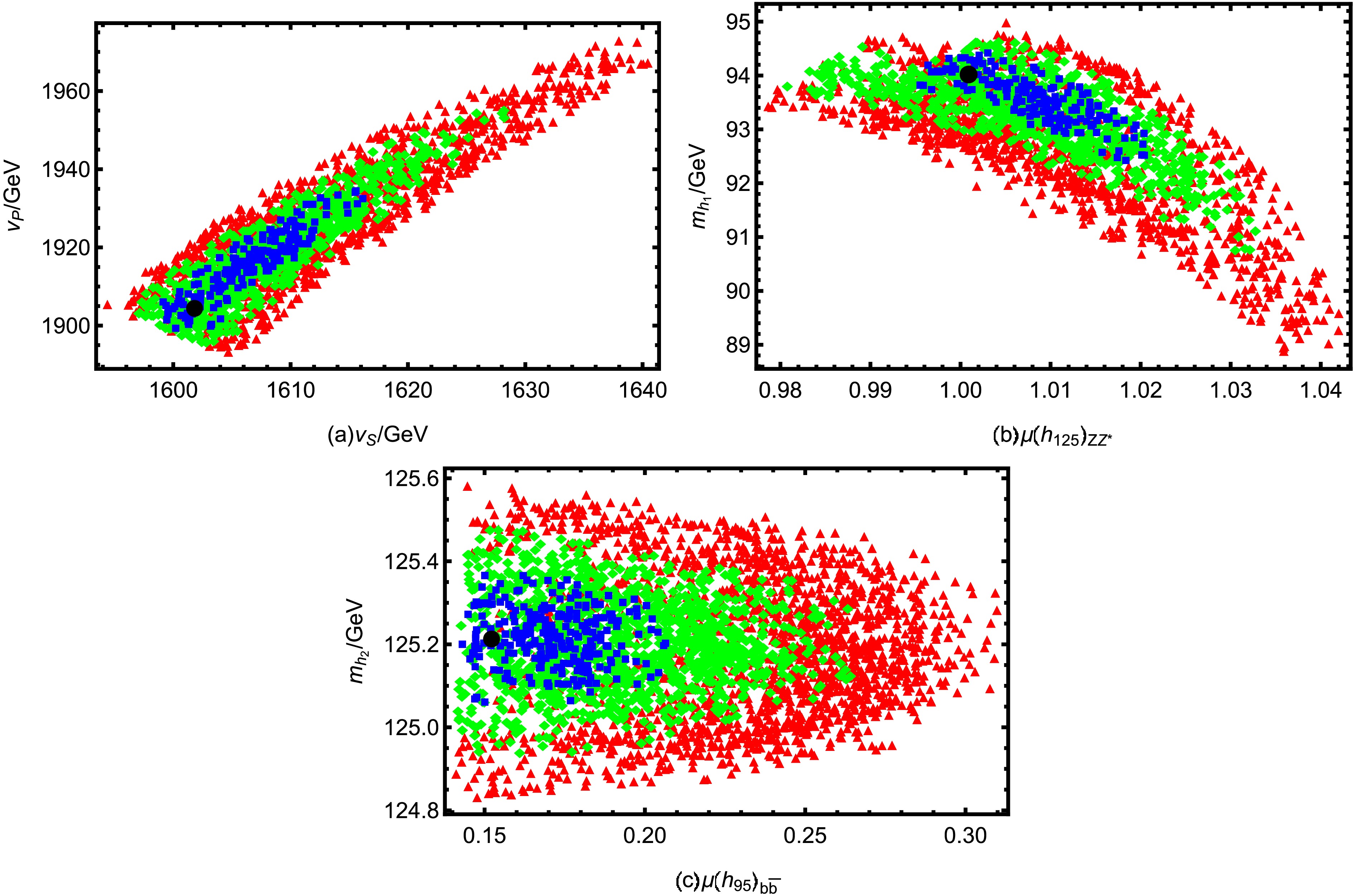
Figure 4. The symbols denote the
$ \chi^2 $ confidence regions: • marks the best-fit point ($ \chi^2_{\rm{min}} = 4.39 $ ), ■ the$ 1\sigma $ region ($ \chi^2 \leq 6.69 $ ), ♦ the$ 1 $ -$ 2\sigma $ region ($ 6.69 \lt \chi^2 \leq 10.57 $ ), and ▲ the$ 2 $ -$ 3\sigma $ region ($ 10.57 \lt \chi^2 \leq 16.22 $ ).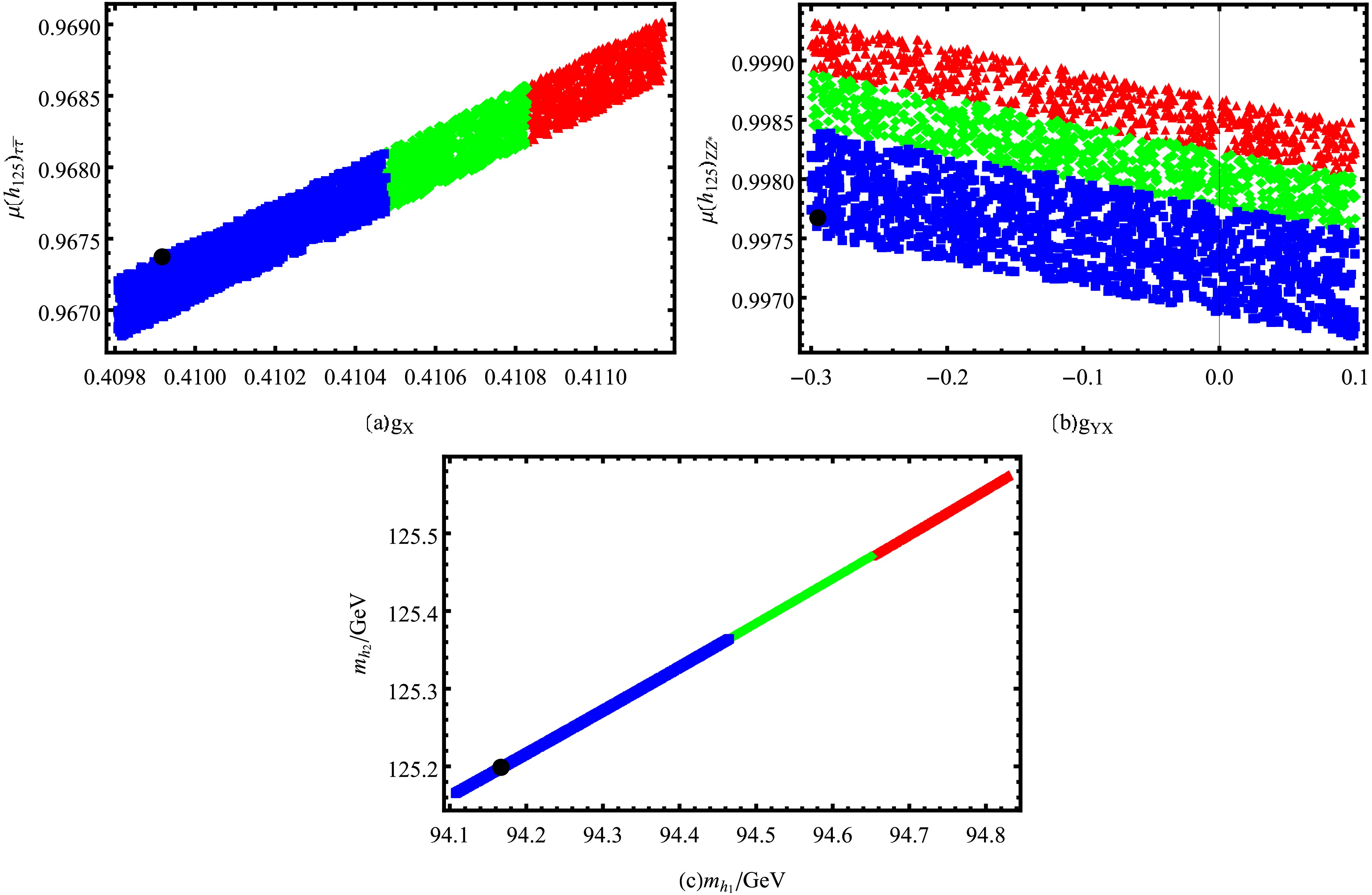
Figure 5. The symbols denote the
$ \chi^2 $ confidence regions: • marks the best-fit point ($ \chi^2_{\rm{min}} = 4.41 $ ); ■ the$ 1\sigma $ region ($ \chi^2 \leq 6.71 $ ); ♦ the$ 1 $ -$ 2\sigma $ region ($ 6.71 \lt \chi^2 \leq 10.59 $ ); and ▲ the$ 2 $ -$ 3\sigma $ region ($ 10.59 \lt \chi^2 \leq 16.24 $ ). -
The gauge group of the
$ U(1)_X $ VLFM is$ S U(3)_C \otimes S U(2)_L \otimes U(1)_Y \otimes U(1)_X $ . To construct the$ U(1)_X $ VLFM, the field content of the SM is extended to include three generations of right-handed neutrino fields$ \nu_R $ , two singlet Higgs fields ϕ and S, and one generation of vector-like quark, lepton, and neutrino fields. The singlet Higgs fields ϕ and S are responsible for the spontaneous breaking of the additional$ U(1)_X $ gauge symmetry and for generating the masses of the vector-like fermions. The inclusion of right-handed neutrinos allows light neutrino masses to be generated at tree level via the seesaw mechanism. After spontaneous symmetry breaking, the neutral CP-even components of$ H,\; \phi $ , and S mix, forming a$ 3\times3 $ mass-squared matrix in the scalar sector. Loop corrections from the vector-like fermions can modify the scalar mass spectrum, allowing the model to accommodate both the SM-like Higgs boson at 125 GeV and a lighter scalar state near 95 GeV.The scalar sector of the
$ U(1)_X $ VLFM consists of one$ S U(2)_L $ Higgs doublet H and two singlet Higgs fields ϕ and S. Their explicit forms are given below:$ \begin{aligned}[b]& H=\left(\begin{array}{c}H^0\\H^-\end{array}\right), \; \; \; \; \; \; H^0={1\over\sqrt{2}}\Big(v+\phi_H+{\rm i}\sigma_H\Big), \\& \phi={1\over\sqrt{2}}\Big(v_P+\phi_P+{\rm i}\sigma_P\Big),\; \; \; \; \; \; S={1\over\sqrt{2}}\Big(v_S+\phi_S+{\rm i}\sigma_S\Big), \end{aligned} $
(6) where v,
$ v_P $ , and$ v_S $ denote the vacuum expectation values (VEVs) of the Higgs superfields H, ϕ, and S, respectively.The two scalars play distinct roles in fermion mass generation: the VEV
$ v_P $ of ϕ primarily generates the masses of vector-like fermions, while the VEV$ v_S $ of S governs the mixing between third-generation SM fermions and their vector-like counterparts. In the neutrino sector, both$ v_P $ and$ v_S $ contribute to neutrino masses via a seesaw mechanism. Therefore, two$ U(1)_X $ Higgs scalars are required to obtain a realistic fermion mass spectrum and mixing structure. Introducing two singlet scalars also enlarges the parameter space, providing sufficient flexibility to simultaneously accommodate the 95 GeV and 125 GeV scalar states and to achieve a good fit to experimental data.Although not required for anomaly cancellation, right-handed neutrinos are included to generate neutrino masses. Their contribution to the 95 GeV scalar signal is subleading, entering only through loop corrections to the scalar effective potential. Hence, their primary role is to provide a viable mechanism for light neutrino masses.
The scalar potential and Yukawa interactions relevant to the Higgs and vector-like fermion sectors can be expressed as
$ \begin{aligned}[b] {\cal{L}}=\;&-\mu^2_H H^\dagger H-\mu^2_P |\phi|^2 -\mu^2_X |S|^2+\lambda_H(H^\dagger H)^2+\lambda_P |\phi|^4 +\lambda_X |S|^4\\& +\lambda_{HP}(H^\dagger H)|\phi|^2+\lambda_{HX}(H^\dagger H)|S|^2+\lambda_{PX}|S|^2|\phi|^2\\&-S d^*_{XL,k}Y^*_{XD,jk}d_{R,j}-S u^*_{R,j}Y_{XU,jk}u_{XL,k}-S e^*_{XL,k}Y^*_{XE,jk}e_{R,j}\\&-S \nu^*_{R,j}Y_{XN,jk}\nu_{XL,k}-{\rm h.c.}\\ & -\phi d^*_{XL,k}Y^*_{PD,jk}d_{XR,j}-\phi u^*_{XR,j}Y_{PU,jk}u_{XL,k}-\phi e^*_{XL,k}Y^*_{PE,jk}e_{XR,j}\\ & -\phi \nu^*_{XR,j}Y_{PN,jk}\nu_{XL,k}-{\rm h.c.}\\ & -Y^*_{u,jk}\bar q_{L,k}H u_{R,j}+Y^*_{d,jk}\bar q_{L,k}\tilde{H} d_{R,j}+Y^*_{e,jk}\bar l_{k}\tilde{H} e_{R,j}+{\rm h.c.} \end{aligned} $
(7) The field content beyond the SM and the charge assignments of the
$ U(1)_X $ VLFM are presented in Table 1, where$ Y^Y $ and$ Y^X $ denote the$ U(1)_Y $ and$ U(1)_X $ gauge charges, respectively. As discussed in Ref. [46], the SM is free of gauge anomalies. In the extended$ U(1)_X $ VLFM, a single generation of vector-like fermions is introduced to preserve this anomaly-free structure. The corresponding anomaly-cancellation conditions can be verified as follows:Field $ S U(3)_C $ $ S U(2)_L $ $ U(1)_Y $ $ U(1)_X $ ϕ 1 1 0 $ Q_a+Q_b $ S 1 1 0 $ Q_a $ $ \nu_R $ 1 1 0 0 $ d_{XL} $ 3 1 –1/3 $ Q_a $ $ u_{XL} $ 3 1 2/3 $ -Q_a $ $ d_{XR} $ $ \bar{3} $ 1 1/3 $ Q_b $ $ u_{XR} $ $ \bar{3} $ 1 –2/3 $ -Q_b $ $ e_{XL} $ 1 1 –1 $ Q_a $ $ \nu_{XL} $ 1 1 0 $ -Q_a $ $ e_{XR} $ 1 1 1 $ Q_b $ $ \nu_{XR} $ 1 1 0 - $ Q_b $ Table 1. Properties of the new particles introduced in the model.
1. Pure gauge anomalies involving three
$ S U(3)_C $ or three$ S U(2)_L $ gauge bosons vanish exactly as in the SM.2. Mixed anomalies that contain one
$ S U(3)_C $ or one$ S U(2)_L $ gauge boson are proportional to the traces$ {\rm Tr}[t^a]=0 $ or$ {\rm Tr}[\tau^a]=0 $ and hence also vanish.3. The mixed anomalies with one
$ U(1)_Y $ or$ U(1)_X $ gauge boson and two$ S U(3)_C $ bosons are proportional to the group-theoretical factors$ {\rm Tr}[t^at^bY^Y]=\dfrac{1}{2}\delta^{ab}\sum_q Y^Y_q $ or${\rm Tr}[t^at^bY^X]=\dfrac{1}{2}\delta^{ab}\sum_q Y^X_q $ .4. Similarly, the mixed anomalies involving one
$ U(1)_Y $ or$ U(1)_X $ gauge boson and two$ S U(2)_L $ bosons are proportional to$ {\rm Tr}[\tau^a\tau^bY^Y]=\dfrac{1}{2}\delta^{ab}\sum_{L} Y^Y_{L} $ or${\rm Tr}[\tau^a\tau^bY^X]= \dfrac{1}{2}\delta^{ab}\sum_{L} Y^X_{L} $ .5. The pure Abelian anomalies containing three
$ U(1) $ gauge bosons can be categorized into four types:$ \begin{array}{l} {\rm Tr}[Y^YY^YY^Y]=\sum\limits_n(Y^Y_n)^3,\; \; \; \; \; \; \; \; \; \; \; {\rm Tr}[Y^XY^XY^X]=\sum\limits_n(Y^X_n)^3,\\ {\rm Tr}[Y^XY^YY^Y]=\sum\limits_nY^X_n(Y^Y_n)^2,\; \; \; \; \; \; {\rm Tr}[Y^YY^XY^X]=\sum\limits_nY^Y_n(Y^X_n)^2. \end{array} $
(8) 6. Mixed gravitational anomalies involving a single
$ U(1) $ gauge boson are proportional to${\rm Tr}[Y^Y]=\sum_n Y_n^Y $ or$ {\rm Tr}[Y^X]=\sum_n Y_n^X $ .Anomaly structures that do not involve the
$ U(1)_X $ gauge group are identical to those in the SM and are automatically consistent. For the anomaly terms associated with the additional$ U(1)_X $ gauge symmetry, the inclusion of one generation of vector-like fermions ensures their complete cancellation. Therefore, all gauge and mixed gravitational anomalies are successfully canceled in the$ U(1)_X $ VLFM, confirming the theoretical consistency of the model.The coexistence of two Abelian gauge groups,
$ U(1)_Y $ and$ U(1)_X $ , in the$ U(1)_X $ VLFM introduces a feature absent in the SM with a single$ U(1)_Y $ : gauge-kinetic mixing. Even if this mixing is set to zero at$ M_{\rm GUT} $ , it can be radiatively generated through RGEs.The covariant derivative of this model takes the general form:
$ D_\mu=\partial_\mu- {\rm i} \left(\begin{array}{cc}Y^Y,&Y^X\end{array}\right) \left(\begin{array}{cc}g_{Y},&g{'}_{{YX}}\\g{'}_{{XY}},&g{'}_{{X}}\end{array}\right) \left(\begin{array}{c}A_{\mu}^{\prime Y} \\ A_{\mu}^{\prime X}\end{array}\right)\;, $
(9) we redefine the gauge fields as
$ B_\mu = g_Y A_\mu^{'Y} + g'_{YX} A_\mu^{'X}, \quad B'_\mu = g'_{XY} A_\mu^{'Y} + g'_X A_\mu^{'X}. $
(10) The gauge fields
$ B_\mu $ and$ B_\mu' $ have canonical kinetic terms.$ \begin{aligned}[b]& -\frac{1}{4} B_{\mu\nu} B^{\mu\nu} - \frac{1}{4} B'_{\mu\nu} B^{\prime\mu\nu}.\\& B_{\mu \nu} = \partial_\mu B_\nu - \partial_\nu B_\mu, \quad B'_{\mu \nu} = \partial'_\mu B_\nu - \partial'_\nu B_\mu. \end{aligned} $
(11) By substituting these redefinitions into the kinetic terms and expanding them, one obtains the standard form.
$ \begin{aligned}[b]& {\cal{L}}_{\text{kin}} = -\frac{1}{4} F_{\mu\nu} F^{\mu\nu} - \frac{1}{4} F'_{\mu\nu} F'^{\mu\nu} - \frac{\epsilon}{4} F_{\mu\nu} F'^{\mu\nu}\\& F_{\mu \nu} = \partial_\mu A_\nu^{'Y} - \partial_\nu A_\mu^{'Y}, \quad F'_{\mu \nu} = \partial_\mu A_\nu^{'X} - \partial_\nu A_\mu^{'X}. \end{aligned} $
(12) where the kinetic-mixing parameter ϵ is given by:
$ \epsilon = \frac{2\bigl(g'_X g'_{YX} + g'_{XY} g_Y\bigr)} {\sqrt{\bigl(g_X'^2 + g_{XY}'^2 \bigr)\bigl(g_Y^2 + g_{YX}'^2 \bigr)}}. $
(13) This expression gives the explicit relationship between
$ g'_{YX} $ ,$ g'_{XY} $ , and the kinetic-mixing parameter ϵ.$ A_{\mu}^{\prime Y} $ and$ A_{\mu}^{\prime X} $ denote the gauge fields associated with$ U(1)_Y $ and$ U(1)_X $ , while$ Y^Y $ and$ Y^X $ denote the corresponding charges. In the unbroken phase, an appropriate basis rotation can be performed in gauge-field space. Introducing a transformation matrix R, the gauge-coupling matrix can be brought into an upper-triangular form:$ \left(\begin{array}{cc}g_{Y},&g{'}_{{YX}}\\g{'}_{{XY}},&g{'}_{{X}}\end{array}\right) R^T=\left(\begin{array}{cc}g_{1},&g_{{YX}}\\0,&g_{{X}}\end{array}\right)\;. $
(14) Consequently, the
$ U(1) $ gauge fields are redefined as follows:$ R\left(\begin{array}{c}A_{\mu}^{\prime Y} \\ A_{\mu}^{\prime X}\end{array}\right) =\left(\begin{array}{c}A_{\mu}^{Y} \\ A_{\mu}^{X}\end{array}\right)\;. $
(15) At tree level, the neutral gauge bosons
$ A^Y_\mu $ ,$ V^3_\mu $ , and$ A^X_\mu $ mix, resulting in a nondiagonal mass matrix in the basis$ (A^Y_\mu, V^3_\mu, A^X_\mu) $ , which can be written as$ \left(\begin{array}{*{20}{c}} \dfrac{1}{4}g_{1}^2 v^2 &\; \; -\dfrac{1}{4}g_{1}g_{2} v^2 & \; \; \dfrac{1}{4}g_{1}g_{{YX}} v^2 \\ -\dfrac{1}{4}g_{1}g_{2} v^2 &\; \; \dfrac{1}{4}g_{2}^2 v^2 & \; \; -\dfrac{1}{4}g_{2}g_{{YX}} v^2\\ \dfrac{1}{4}g_{1}g_{{YX}} v^2 &\; \; -\dfrac{1}{4}g_{2}g_{{YX}} v^2 &\; \; \dfrac{1}{4}g_{{YX}}^2 v^2+\dfrac{1}{4}g_{{X}}^2\xi^2 \end{array}\right). $
(16) Here,
$ \xi^2=4(Q_a + Q_b)^2 v^2_P+ 4Q^2_a v^2_S $ . The diagonalization of the matrix above can be achieved through a rotation involving the weak mixing angle$ \theta_W $ and an additional angle$ \theta_W' $ .$\begin{aligned}[b] \left(\begin{array}{*{20}{c}} \gamma_\mu\\ Z_\mu\\ Z'_\mu \end{array}\right)=\;& \left( \begin{array}{*{20}{c}} \cos\theta_{W} & \sin\theta_{W} & 0 \\ -\sin\theta_{W}\cos\theta_{W}' & \cos\theta_{W}\cos\theta_{W}' & \sin\theta_{W}' \\ \sin\theta_{W}\sin\theta_{W}' & -\cos\theta_{W}'\sin\theta_{W}' & \cos\theta_{W}' \end{array}\right)\\& \times\left(\begin{array}{*{20}{c}} A^Y_\mu\\ V^3_\mu\\ A^{X}_\mu \end{array}\right).\end{aligned} $
(17) The explicit expression for
$ \sin^2\theta_W' $ is given by$\begin{aligned}[b]& \sin^2\theta_{W}'=\frac{1}{2}\\&-\frac{(g_{{YX}}^2-g_{1}^2-g_{2}^2)v^2+ g_{X}^2\xi^2}{2\sqrt{(g_{{YX}}^2+g_{1}^2+g_{2}^2)^2v^4+2g_{X}^2(g_{{YX}}^2-g_{1}^2-g_{2}^2)v^2\xi^2+g_{X}^4\xi^4}},\end{aligned} $
(18) where
$ \sin\theta_W' $ is of order$ {\cal{O}}(10^{-3}) $ [47−49].The new mixing angle
$ \theta_{W}^\prime $ appears in the couplings involving Z and$ Z^{\prime} $ . The exact eigenvalues of Eq. (16) are given by$ \begin{aligned}[b]& m_\gamma^2=0,\\ &m_{Z,{Z^{'}}}^2=\frac{1}{8}\Big((g_{1}^2+g_2^2+g_{YX}^2)v^2+g_{X}^2 \xi^2 \\& \qquad\;\ \ \ \mp\sqrt{[(g_{1}^2+g_2^2+g_{YX}^2)v^2+g_{X}^2 \xi^2]^2-4(g^2_1+g^2_2)g^2_X v^2 \xi^2}\Big). \end{aligned} $
(19) In our model, the mixing between the Z boson and the TeV-scale
$ Z' $ induces corrections to the Z boson mass. Expanding the exact expression in Eq. (19) in the limit$ v^2 \ll \xi^2 $ , we obtain:$ m^2_Z\approx \frac{(g_1^2 + g_2^2)v^2}{4} - \frac{(g_1^2 + g_2^2) g_{YX}^2}{4 g_X^2} \cdot \frac{v^4}{\xi^2}, $
(20) where
$ \xi^2 = 4(Q_a+Q_b)^2 v_P^2 + 4Q_a^2 v_S^2 $ , with$ Q_a=Q_b=1 $ .The leading term reproduces the SM result; a further estimate yields
$ \frac{\delta m^2_Z}{m^2_Z} \sim \frac{g_{YX}^2}{g_X^2} \cdot \frac{v^2}{\xi^2} =\frac{g_{YX}^2}{g_X^2} \cdot \frac{v^2}{16 v_P^2 + 4 v_S^2} \sim{\cal{O}}(10^{-5}). $
(21) For the W-boson mass, because the new scalar fields are singlets under
$ S U(2)_L $ and there are no charged scalar states (such as$ H^{\pm} $ ), the W boson does not mix with them. Furthermore, electroweak symmetry breaking is dominated by the SM Higgs doublet; therefore, scalar mixing does not introduce additional corrections to the W mass. Its tree-level mass expression remains unchanged$ m_W^2 = \frac{g_2^2 v^2}{4}. $
(22) It is not affected by the mixing effects discussed above in this model.
Based on the above analysis, within the parameter regions considered in the numerical figures, the corrections to
$ m_Z $ and$ m_W $ are negligible; thus, they are not included in the fit. -
The one-loop effective potential can be expressed as follows:
$ V_{\rm Total}=V_{\rm Tree}+\Delta V. $
(23) Here,
$ V_{\rm Tree} $ denotes the tree-level potential, whereas$ \Delta V $ represents the one-loop correction.The simplified Higgs potential at tree level is given as follows:
$ \begin{aligned}[b] V_{\rm Tree}=\;&\mu^2_H H^\dagger H+\mu^2_P |\phi|^2 +\mu^2_X |S|^2-\lambda_H(H^\dagger H)^2\\&-\lambda_P |\phi|^4 -\lambda_X |S|^4 -\lambda_{HP}(H^\dagger H)|\phi|^2\\&-\lambda_{HX}(H^\dagger H)|S|^2-\lambda_{PX}|S|^2|\phi|^2. \end{aligned} $
(24) We also derive the corresponding tadpole equations at tree level.
$ 2\lambda_H v^2-2\mu^2_H +\lambda_{HP} v^2_P+\lambda_{HX} v^2_S=0, $
(25) $ 2\lambda_X v^2_S-2\mu^2_X +\lambda_{HX} v^2+\lambda_{PX} v^2_P=0, $
(26) $ 2\lambda_P v^2_P-2\mu^2_P +\lambda_{HP} v^2+\lambda_{PX} v^2_S=0. $
(27) In addition, the tree-level mass-squared matrix for the CP-even Higgs fields
$ ({\phi}_{H}, {\phi}_{S}, {\phi}_{P}) $ is presented$ M^2_{h,\rm tree} = \left( \begin{array}{ccc} m_{{\phi}_{H}{\phi}_{H}} &-\lambda_{HX}v v_S &-\lambda_{HP}v v_P \\ -\lambda_{HX}v v_S &m_{{\phi}_{S}{\phi}_{S}} &-\lambda_{PX}v_P v_S \\ -\lambda_{HP}v v_P &-\lambda_{PX}v_P v_S &m_{{\phi}_{P}{\phi}_{P}} \end{array} \right), $
(28) with the diagonal entries defined as
$ m_{\phi_{H}\phi_{H}}=\frac{1}{2}\Big(-6\lambda_H v^2-\lambda_{HP}v^2_P-\lambda_{HX}v^2_S\Big)+\mu^2_H, $
(29) $ m_{\phi_{S}\phi_{S}} = \frac{1}{2}\Big(-6\lambda_X v^2_S-\lambda_{HX}v^2-\lambda_{PX}v^2_P\Big)+\mu^2_X, $
(30) $ m_{\phi_{P}\phi_{P}} = \frac{1}{2}\Big(-6\lambda_P v_P^2-\lambda_{HP}v^2-\lambda_{PX}v^2_S\Big)+\mu^2_P. $
(31) Within dimensional regularization and the
$ \overline{\text{MS}} $ renormalization scheme in the Landau gauge, the effective Higgs potential acquires one-loop corrections, with$ \Delta V $ given by the Coleman-Weinberg form [50−52]$ \Delta V=\sum\limits_i\frac{n_i}{64\pi^2}m_i^4(\phi_H,\phi_S,\phi_P)\bigg( \log\frac{m_i^2(\phi_H,\phi_S,\phi_P)}{Q^2}-\frac{3}{2}\bigg). $
(32) The renormalization scale Q is chosen to be of order TeV. The degrees of freedom
$ n_i $ for each mass eigenstate are assigned as follows: –12 for quarks, –4 for charged leptons, –2 for neutrinos, 6 for the W boson, 3 for the Z boson, and, similarly, for the$ Z^\prime $ boson. The explicit form of the one-loop correction to the potential reads$ \Delta V = \sum\limits_{f=t,b,\tau} V_f + \sum\limits_{F=t',b',\tau'} V_F +V_{\nu'}+ V_W + V_Z + V_{Z'}. $
(33) Here,
$ V_f $ ($ f=t,b,\tau $ ) and$ V_F $ ($ F=t',b',\tau' $ ) denote the one-loop effective potential contributions from the SM fermions and the vector-like fermions, respectively.$ V_{\nu'} $ represents the contribution from the heavy neutrino sector.$ V_W $ ,$ V_Z $ , and$ V_{Z'} $ correspond to the contributions from the W boson, Z boson, and the$ Z^\prime $ boson.In the
$ U(1)_X $ VLFM, the fermion mass matrices arise from Yukawa interactions and are defined in the gauge-eigenstate basis. For instance, the down-type quarks are written in the bases$ (d_L, d_{XL}) $ and$ (d^*_R, d^*_{XR}) $ , leading to the mass matrix$ m_d = \left( \begin{array}{cc} \dfrac{1}{\sqrt{2}}v Y^T_d &0\\ \dfrac{1}{\sqrt{2}}v_S Y^T_{XD} &\dfrac{1}{\sqrt{2}}v_P Y^T_{PD}\end{array} \right). $
(34) Similarly, the up-type quarks and the charged leptons are expressed in the corresponding bases
$ (u_L, u_{XL}), (u^*_R, u^*_{XR}) $ and$ (e_L, e_{XL}), (e^*_R, e^*_{XR}) $ , respectively, with mass matrices:$ \begin{aligned}[b]& m_u = \left( \begin{array}{cc} \dfrac{1}{\sqrt{2}}v Y^T_u &0\\ \dfrac{1}{\sqrt{2}}v_S Y^T_{XU} &\dfrac{1}{\sqrt{2}}v_P Y^T_{PU}\end{array}\right),\\& m_e = \left( \begin{array}{cc} \dfrac{1}{\sqrt{2}}v Y^T_e &0\\ \dfrac{1}{\sqrt{2}}v_S Y^T_{XE} &\dfrac{1}{\sqrt{2}}v_P Y^T_{PE}\end{array} \right).\end{aligned} $
(35) These Dirac-type mass matrices are diagonalized by bi-unitary transformations.
$ U_L^{f,*}\, m_f \, U_R^{f,\dagger} = m_f^{\text{diag}}, \qquad f = d,u,e, $
(36) where
$ U_L^f $ and$ U_R^f $ are unitary matrices acting on the left- and right-handed fermion fields, respectively.The neutrino sector, in the basis
$ (\nu_L, \nu^*_R, \nu_{XL}, \nu^*_{XR}) $ , has the mass matrix:$ m_{\nu} = \left( \begin{array}{cccc} 0 &\dfrac{1}{\sqrt 2}v Y^T_v & 0 &0 \\ \dfrac{1}{\sqrt 2}v Y_v &0& \dfrac{1}{\sqrt 2}v_S Y_{XN} &0 \\ 0 &\dfrac{1}{\sqrt 2}v_S Y^T_{XN}& 0 &\dfrac{1}{\sqrt 2}v_P Y^T_{PN}\\ 0 &0& \dfrac{1}{\sqrt 2}v_P Y_{PN} &0\end{array} \right). $
(37) Being of Majorana type, the neutrino mass matrix is diagonalized by a single unitary matrix
$ U^V $ as$ U^{V,*} m_\nu U^{V,\dagger} = m_\nu^{\text{diag}}. $
(38) The one-loop minimization conditions for the total effective potential
$ V_{\rm Total} $ within the$ U(1)_X $ VLFM are given by:$ \left \langle \frac{\partial V_{\rm Total}}{\partial \phi_H} \right \rangle= \left \langle \frac{\partial V_{\rm Total}}{\partial \phi_S} \right \rangle= \left \langle \frac{\partial V_{\rm Total}}{\partial \phi_P} \right \rangle=0. $
(39) Because the analytic forms of these conditions are cumbersome, we solve them numerically. Explicit expressions for the down-type quark sector are provided in Appendix A for reference.
The one-loop contributions to the effective potential
$ V_{\rm Total} $ give rise to radiative corrections in the mass-squared matrix of the CP-even Higgs sector$ M^2_{{\rm Total},h}=M^2_{{\rm Tree},h}+\Delta M^2_h. $
(40) The elements of the corrected mass-squared matrix
$ M^2_{{\rm Total},h,ij} $ are obtained from the second derivatives of the effective potential$ V_{{\rm Total}} $ .$ M^2_{{\rm Total},h,ij}=\Big\langle\frac{\partial^2V_{\rm Total}}{\partial \phi_i \partial \phi_j}\Big|_{\phi_i,\phi_j=\phi_H,\phi_S,\phi_P}\Big\rangle. $
(41) Diagonalization of
$ M^2_{{\rm Total},h} $ yields the squares of the mass eigenvalues$ m_{{h_n}} $ ($ n=1,2,3 $ ), which we order as$ m_{{h_1}} \lt m_{{h_2}} \lt m_{{h_3}} $ . In this work we identify the lightest eigenstate,$ h_1 $ , with the Higgs-like excess observed near 95 GeV, and the next-to-lightest eigenstate,$ h_2 $ , with the SM-like Higgs boson at 125 GeV. -
The one-loop effective potential can be expressed as follows:
$ V_{Total}=V_{Tree}+\Delta V. $
(23) Here,
$ V_{Tree} $ denotes the tree-level potential, whereas$ \Delta V $ represents the one-loop correction.The simplified Higgs potential at tree level is given as follows:
$ \begin{aligned}[b] V_{Tree}=\;&\mu^2_H H^\dagger H+\mu^2_P |\phi|^2 +\mu^2_X |S|^2-\lambda_H(H^\dagger H)^2\\&-\lambda_P |\phi|^4 -\lambda_X |S|^4 -\lambda_{HP}(H^\dagger H)|\phi|^2\\&-\lambda_{HX}(H^\dagger H)|S|^2-\lambda_{PX}|S|^2|\phi|^2. \end{aligned} $
(24) We also derive the corresponding tadpole equations at tree level.
$ 2\lambda_H v^2-2\mu^2_H +\lambda_{HP} v^2_P+\lambda_{HX} v^2_S=0, $
(25) $ 2\lambda_X v^2_S-2\mu^2_X +\lambda_{HX} v^2+\lambda_{PX} v^2_P=0, $
(26) $ 2\lambda_P v^2_P-2\mu^2_P +\lambda_{HP} v^2+\lambda_{PX} v^2_S=0. $
(27) In addition, the tree-level mass-squared matrix for the CP-even Higgs fields
$ ({\phi}_{H}, {\phi}_{S}, {\phi}_{P}) $ is presented.$ M^2_{h,tree} = \left( \begin{array}{ccc} m_{{\phi}_{H}{\phi}_{H}} &-\lambda_{HX}v v_S &-\lambda_{HP}v v_P \\ -\lambda_{HX}v v_S &m_{{\phi}_{S}{\phi}_{S}} &-\lambda_{PX}v_P v_S \\ -\lambda_{HP}v v_P &-\lambda_{PX}v_P v_S &m_{{\phi}_{P}{\phi}_{P}} \end{array} \right), $
(28) with the diagonal entries defined as
$ m_{\phi_{H}\phi_{H}}=\frac{1}{2}\Big(-6\lambda_H v^2-\lambda_{HP}v^2_P-\lambda_{HX}v^2_S\Big)+\mu^2_H, $
(29) $ m_{\phi_{S}\phi_{S}} = \frac{1}{2}\Big(-6\lambda_X v^2_S-\lambda_{HX}v^2-\lambda_{PX}v^2_P\Big)+\mu^2_X, $
(30) $ m_{\phi_{P}\phi_{P}} = \frac{1}{2}\Big(-6\lambda_P v_P^2-\lambda_{HP}v^2-\lambda_{PX}v^2_S\Big)+\mu^2_P. $
(31) Within dimensional regularization and the
$ \overline{\text{MS}} $ renormalization scheme in the Landau gauge, the effective Higgs potential acquires one-loop corrections, with$ \Delta V $ given by the Coleman-Weinberg form [45−47]$ \Delta V=\sum\limits_i\frac{n_i}{64\pi^2}m_i^4(\phi_H,\phi_S,\phi_P)\Big( \log\frac{m_i^2(\phi_H,\phi_S,\phi_P)}{Q^2}-\frac{3}{2}\Big). $
(32) The renormalization scale Q is chosen to be of order TeV. The degrees of freedom
$ n_i $ for each mass eigenstate are assigned as follows: -12 for quarks, -4 for charged leptons, -2 for neutrinos, 6 for the W boson, 3 for the Z boson, and, similarly, for the$ Z^\prime $ boson. The explicit form of the one-loop correction to the potential reads$ \Delta V = \sum\limits_{f=t,b,\tau} V_f + \sum\limits_{F=t',b',\tau'} V_F +V_{\nu'}+ V_W + V_Z + V_{Z'}. $
(33) Here,
$ V_f $ ($ f=t,b,\tau $ ) and$ V_F $ ($ F=t',b',\tau' $ ) denote the one-loop effective potential contributions from the SM fermions and the vector-like fermions, respectively.$ V_{\nu'} $ represents the contribution from the heavy neutrino sector.$ V_W $ ,$ V_Z $ , and$ V_{Z'} $ correspond to the contributions from the W boson, Z boson, and the$ Z^\prime $ boson.In the
$ U(1)_X $ VLFM, the fermion mass matrices arise from Yukawa interactions and are defined in the gauge-eigenstate basis. For instance, the down-type quarks are written in the bases$ (d_L, d_{XL}) $ and$ (d^*_R, d^*_{XR}) $ , leading to the mass matrix$ m_d = \left( \begin{array}{cc} \dfrac{1}{\sqrt{2}}v Y^T_d &0\\ \dfrac{1}{\sqrt{2}}v_S Y^T_{XD} &\dfrac{1}{\sqrt{2}}v_P Y^T_{PD}\end{array} \right). $
(34) Similarly, the up-type quarks and the charged leptons are expressed in the corresponding bases
$ (u_L, u_{XL}), (u^*_R, u^*_{XR}) $ and$ (e_L, e_{XL}), (e^*_R, e^*_{XR}) $ , respectively, with mass matrices:$ \begin{aligned}[b]& m_u = \left( \begin{array}{cc} \dfrac{1}{\sqrt{2}}v Y^T_u &0\\ \dfrac{1}{\sqrt{2}}v_S Y^T_{XU} &\dfrac{1}{\sqrt{2}}v_P Y^T_{PU}\end{array}\right),\\& m_e = \left( \begin{array}{cc} \dfrac{1}{\sqrt{2}}v Y^T_e &0\\ \dfrac{1}{\sqrt{2}}v_S Y^T_{XE} &\dfrac{1}{\sqrt{2}}v_P Y^T_{PE}\end{array} \right).\end{aligned} $
(35) These Dirac-type mass matrices are diagonalized by bi-unitary transformations.
$ U_L^{f,*}\, m_f \, U_R^{f,\dagger} = m_f^{\text{diag}}, \qquad f = d,u,e, $
(36) where
$ U_L^f $ and$ U_R^f $ are unitary matrices acting on the left- and right-handed fermion fields, respectively.The neutrino sector, in the basis
$ (\nu_L, \nu^*_R, \nu_{XL}, \nu^*_{XR}) $ , has the mass matrix:$ m_{\nu} = \left( \begin{array}{cccc} 0 &\dfrac{1}{\sqrt 2}v Y^T_v & 0 &0 \\ \dfrac{1}{\sqrt 2}v Y_v &0& \dfrac{1}{\sqrt 2}v_S Y_{XN} &0 \\ 0 &\dfrac{1}{\sqrt 2}v_S Y^T_{XN}& 0 &\dfrac{1}{\sqrt 2}v_P Y^T_{PN}\\ 0 &0& \dfrac{1}{\sqrt 2}v_P Y_{PN} &0\end{array} \right). $
(37) Being of Majorana type, the neutrino mass matrix is diagonalized by a single unitary matrix
$ U^V $ as$ U^{V,*} m_\nu U^{V,\dagger} = m_\nu^{\text{diag}}. $
(38) The one-loop minimization conditions for the total effective potential
$ V_{Total} $ within the$ U(1)_X $ VLFM are given by:$ \left \langle \frac{\partial V_{Total}}{\partial \phi_H} \right \rangle= \left \langle \frac{\partial V_{Total}}{\partial \phi_S} \right \rangle= \left \langle \frac{\partial V_{Total}}{\partial \phi_P} \right \rangle=0, $
(39) Because the analytic forms of these conditions are cumbersome, we solve them numerically. Explicit expressions for the down-type quark sector are provided in Appendix A for reference.
The one-loop contributions to the effective potential
$ V_{Total} $ give rise to radiative corrections in the mass-squared matrix of the CP-even Higgs sector.$ M^2_{Total,h}=M^2_{Tree,h}+\Delta M^2_h, $
(40) The elements of the corrected mass-squared matrix
$ M^2_{Total,h,ij} $ are obtained from the second derivatives of the effective potential$ V_{{Total}} $ .$ M^2_{Total,h,ij}=\Big\langle\frac{\partial^2V_{Total}}{\partial \phi_i \partial \phi_j}\Big|_{\phi_i,\phi_j=\phi_H,\phi_S,\phi_P}\Big\rangle. $
(41) Diagonalization of
$ M^2_{Total,h} $ yields the squares of the mass eigenvalues$ m_{{h_n}} $ ($ n=1,2,3 $ ), which we order as$ m_{{h_1}} \lt m_{{h_2}} \lt m_{{h_3}} $ . In this work we identify the lightest eigenstate,$ h_1 $ , with the Higgs-like excess observed near 95 GeV, and the next-to-lightest eigenstate,$ h_2 $ , with the SM-like Higgs boson at 125 GeV. -
The one-loop effective potential can be expressed as follows:
$ V_{\rm Total}=V_{\rm Tree}+\Delta V. $
(23) Here,
$ V_{\rm Tree} $ denotes the tree-level potential, whereas$ \Delta V $ represents the one-loop correction.The simplified Higgs potential at tree level is given as follows:
$ \begin{aligned}[b] V_{\rm Tree}=\;&\mu^2_H H^\dagger H+\mu^2_P |\phi|^2 +\mu^2_X |S|^2-\lambda_H(H^\dagger H)^2\\&-\lambda_P |\phi|^4 -\lambda_X |S|^4 -\lambda_{HP}(H^\dagger H)|\phi|^2\\&-\lambda_{HX}(H^\dagger H)|S|^2-\lambda_{PX}|S|^2|\phi|^2. \end{aligned} $
(24) We also derive the corresponding tadpole equations at tree level.
$ 2\lambda_H v^2-2\mu^2_H +\lambda_{HP} v^2_P+\lambda_{HX} v^2_S=0, $
(25) $ 2\lambda_X v^2_S-2\mu^2_X +\lambda_{HX} v^2+\lambda_{PX} v^2_P=0, $
(26) $ 2\lambda_P v^2_P-2\mu^2_P +\lambda_{HP} v^2+\lambda_{PX} v^2_S=0. $
(27) In addition, the tree-level mass-squared matrix for the CP-even Higgs fields
$ ({\phi}_{H}, {\phi}_{S}, {\phi}_{P}) $ is presented$ M^2_{h,\rm tree} = \left( \begin{array}{ccc} m_{{\phi}_{H}{\phi}_{H}} &-\lambda_{HX}v v_S &-\lambda_{HP}v v_P \\ -\lambda_{HX}v v_S &m_{{\phi}_{S}{\phi}_{S}} &-\lambda_{PX}v_P v_S \\ -\lambda_{HP}v v_P &-\lambda_{PX}v_P v_S &m_{{\phi}_{P}{\phi}_{P}} \end{array} \right), $
(28) with the diagonal entries defined as
$ m_{\phi_{H}\phi_{H}}=\frac{1}{2}\Big(-6\lambda_H v^2-\lambda_{HP}v^2_P-\lambda_{HX}v^2_S\Big)+\mu^2_H, $
(29) $ m_{\phi_{S}\phi_{S}} = \frac{1}{2}\Big(-6\lambda_X v^2_S-\lambda_{HX}v^2-\lambda_{PX}v^2_P\Big)+\mu^2_X, $
(30) $ m_{\phi_{P}\phi_{P}} = \frac{1}{2}\Big(-6\lambda_P v_P^2-\lambda_{HP}v^2-\lambda_{PX}v^2_S\Big)+\mu^2_P. $
(31) Within dimensional regularization and the
$ \overline{\text{MS}} $ renormalization scheme in the Landau gauge, the effective Higgs potential acquires one-loop corrections, with$ \Delta V $ given by the Coleman-Weinberg form [50−52]$ \Delta V=\sum\limits_i\frac{n_i}{64\pi^2}m_i^4(\phi_H,\phi_S,\phi_P)\bigg( \log\frac{m_i^2(\phi_H,\phi_S,\phi_P)}{Q^2}-\frac{3}{2}\bigg). $
(32) The renormalization scale Q is chosen to be of order TeV. The degrees of freedom
$ n_i $ for each mass eigenstate are assigned as follows: –12 for quarks, –4 for charged leptons, –2 for neutrinos, 6 for the W boson, 3 for the Z boson, and, similarly, for the$ Z^\prime $ boson. The explicit form of the one-loop correction to the potential reads$ \Delta V = \sum\limits_{f=t,b,\tau} V_f + \sum\limits_{F=t',b',\tau'} V_F +V_{\nu'}+ V_W + V_Z + V_{Z'}. $
(33) Here,
$ V_f $ ($ f=t,b,\tau $ ) and$ V_F $ ($ F=t',b',\tau' $ ) denote the one-loop effective potential contributions from the SM fermions and the vector-like fermions, respectively.$ V_{\nu'} $ represents the contribution from the heavy neutrino sector.$ V_W $ ,$ V_Z $ , and$ V_{Z'} $ correspond to the contributions from the W boson, Z boson, and the$ Z^\prime $ boson.In the
$ U(1)_X $ VLFM, the fermion mass matrices arise from Yukawa interactions and are defined in the gauge-eigenstate basis. For instance, the down-type quarks are written in the bases$ (d_L, d_{XL}) $ and$ (d^*_R, d^*_{XR}) $ , leading to the mass matrix$ m_d = \left( \begin{array}{cc} \dfrac{1}{\sqrt{2}}v Y^T_d &0\\ \dfrac{1}{\sqrt{2}}v_S Y^T_{XD} &\dfrac{1}{\sqrt{2}}v_P Y^T_{PD}\end{array} \right). $
(34) Similarly, the up-type quarks and the charged leptons are expressed in the corresponding bases
$ (u_L, u_{XL}), (u^*_R, u^*_{XR}) $ and$ (e_L, e_{XL}), (e^*_R, e^*_{XR}) $ , respectively, with mass matrices:$ \begin{aligned}[b]& m_u = \left( \begin{array}{cc} \dfrac{1}{\sqrt{2}}v Y^T_u &0\\ \dfrac{1}{\sqrt{2}}v_S Y^T_{XU} &\dfrac{1}{\sqrt{2}}v_P Y^T_{PU}\end{array}\right),\\& m_e = \left( \begin{array}{cc} \dfrac{1}{\sqrt{2}}v Y^T_e &0\\ \dfrac{1}{\sqrt{2}}v_S Y^T_{XE} &\dfrac{1}{\sqrt{2}}v_P Y^T_{PE}\end{array} \right).\end{aligned} $
(35) These Dirac-type mass matrices are diagonalized by bi-unitary transformations.
$ U_L^{f,*}\, m_f \, U_R^{f,\dagger} = m_f^{\text{diag}}, \qquad f = d,u,e, $
(36) where
$ U_L^f $ and$ U_R^f $ are unitary matrices acting on the left- and right-handed fermion fields, respectively.The neutrino sector, in the basis
$ (\nu_L, \nu^*_R, \nu_{XL}, \nu^*_{XR}) $ , has the mass matrix:$ m_{\nu} = \left( \begin{array}{cccc} 0 &\dfrac{1}{\sqrt 2}v Y^T_v & 0 &0 \\ \dfrac{1}{\sqrt 2}v Y_v &0& \dfrac{1}{\sqrt 2}v_S Y_{XN} &0 \\ 0 &\dfrac{1}{\sqrt 2}v_S Y^T_{XN}& 0 &\dfrac{1}{\sqrt 2}v_P Y^T_{PN}\\ 0 &0& \dfrac{1}{\sqrt 2}v_P Y_{PN} &0\end{array} \right). $
(37) Being of Majorana type, the neutrino mass matrix is diagonalized by a single unitary matrix
$ U^V $ as$ U^{V,*} m_\nu U^{V,\dagger} = m_\nu^{\text{diag}}. $
(38) The one-loop minimization conditions for the total effective potential
$ V_{\rm Total} $ within the$ U(1)_X $ VLFM are given by:$ \left \langle \frac{\partial V_{\rm Total}}{\partial \phi_H} \right \rangle= \left \langle \frac{\partial V_{\rm Total}}{\partial \phi_S} \right \rangle= \left \langle \frac{\partial V_{\rm Total}}{\partial \phi_P} \right \rangle=0. $
(39) Because the analytic forms of these conditions are cumbersome, we solve them numerically. Explicit expressions for the down-type quark sector are provided in Appendix A for reference.
The one-loop contributions to the effective potential
$ V_{\rm Total} $ give rise to radiative corrections in the mass-squared matrix of the CP-even Higgs sector$ M^2_{{\rm Total},h}=M^2_{{\rm Tree},h}+\Delta M^2_h. $
(40) The elements of the corrected mass-squared matrix
$ M^2_{{\rm Total},h,ij} $ are obtained from the second derivatives of the effective potential$ V_{{\rm Total}} $ .$ M^2_{{\rm Total},h,ij}=\Big\langle\frac{\partial^2V_{\rm Total}}{\partial \phi_i \partial \phi_j}\Big|_{\phi_i,\phi_j=\phi_H,\phi_S,\phi_P}\Big\rangle. $
(41) Diagonalization of
$ M^2_{{\rm Total},h} $ yields the squares of the mass eigenvalues$ m_{{h_n}} $ ($ n=1,2,3 $ ), which we order as$ m_{{h_1}} \lt m_{{h_2}} \lt m_{{h_3}} $ . In this work we identify the lightest eigenstate,$ h_1 $ , with the Higgs-like excess observed near 95 GeV, and the next-to-lightest eigenstate,$ h_2 $ , with the SM-like Higgs boson at 125 GeV. -
The one-loop effective potential can be expressed as follows:
$ V_{\rm Total}=V_{\rm Tree}+\Delta V. $
(23) Here,
$ V_{\rm Tree} $ denotes the tree-level potential, whereas$ \Delta V $ represents the one-loop correction.The simplified Higgs potential at tree level is given as follows:
$ \begin{aligned}[b] V_{\rm Tree}=\;&\mu^2_H H^\dagger H+\mu^2_P |\phi|^2 +\mu^2_X |S|^2-\lambda_H(H^\dagger H)^2\\&-\lambda_P |\phi|^4 -\lambda_X |S|^4 -\lambda_{HP}(H^\dagger H)|\phi|^2\\&-\lambda_{HX}(H^\dagger H)|S|^2-\lambda_{PX}|S|^2|\phi|^2. \end{aligned} $
(24) We also derive the corresponding tadpole equations at tree level.
$ 2\lambda_H v^2-2\mu^2_H +\lambda_{HP} v^2_P+\lambda_{HX} v^2_S=0, $
(25) $ 2\lambda_X v^2_S-2\mu^2_X +\lambda_{HX} v^2+\lambda_{PX} v^2_P=0, $
(26) $ 2\lambda_P v^2_P-2\mu^2_P +\lambda_{HP} v^2+\lambda_{PX} v^2_S=0. $
(27) In addition, the tree-level mass-squared matrix for the CP-even Higgs fields
$ ({\phi}_{H}, {\phi}_{S}, {\phi}_{P}) $ is presented$ M^2_{h,\rm tree} = \left( \begin{array}{ccc} m_{{\phi}_{H}{\phi}_{H}} &-\lambda_{HX}v v_S &-\lambda_{HP}v v_P \\ -\lambda_{HX}v v_S &m_{{\phi}_{S}{\phi}_{S}} &-\lambda_{PX}v_P v_S \\ -\lambda_{HP}v v_P &-\lambda_{PX}v_P v_S &m_{{\phi}_{P}{\phi}_{P}} \end{array} \right), $
(28) with the diagonal entries defined as
$ m_{\phi_{H}\phi_{H}}=\frac{1}{2}\Big(-6\lambda_H v^2-\lambda_{HP}v^2_P-\lambda_{HX}v^2_S\Big)+\mu^2_H, $
(29) $ m_{\phi_{S}\phi_{S}} = \frac{1}{2}\Big(-6\lambda_X v^2_S-\lambda_{HX}v^2-\lambda_{PX}v^2_P\Big)+\mu^2_X, $
(30) $ m_{\phi_{P}\phi_{P}} = \frac{1}{2}\Big(-6\lambda_P v_P^2-\lambda_{HP}v^2-\lambda_{PX}v^2_S\Big)+\mu^2_P. $
(31) Within dimensional regularization and the
$ \overline{\text{MS}} $ renormalization scheme in the Landau gauge, the effective Higgs potential acquires one-loop corrections, with$ \Delta V $ given by the Coleman-Weinberg form [50−52]$ \Delta V=\sum\limits_i\frac{n_i}{64\pi^2}m_i^4(\phi_H,\phi_S,\phi_P)\bigg( \log\frac{m_i^2(\phi_H,\phi_S,\phi_P)}{Q^2}-\frac{3}{2}\bigg). $
(32) The renormalization scale Q is chosen to be of order TeV. The degrees of freedom
$ n_i $ for each mass eigenstate are assigned as follows: –12 for quarks, –4 for charged leptons, –2 for neutrinos, 6 for the W boson, 3 for the Z boson, and, similarly, for the$ Z^\prime $ boson. The explicit form of the one-loop correction to the potential reads$ \Delta V = \sum\limits_{f=t,b,\tau} V_f + \sum\limits_{F=t',b',\tau'} V_F +V_{\nu'}+ V_W + V_Z + V_{Z'}. $
(33) Here,
$ V_f $ ($ f=t,b,\tau $ ) and$ V_F $ ($ F=t',b',\tau' $ ) denote the one-loop effective potential contributions from the SM fermions and the vector-like fermions, respectively.$ V_{\nu'} $ represents the contribution from the heavy neutrino sector.$ V_W $ ,$ V_Z $ , and$ V_{Z'} $ correspond to the contributions from the W boson, Z boson, and the$ Z^\prime $ boson.In the
$ U(1)_X $ VLFM, the fermion mass matrices arise from Yukawa interactions and are defined in the gauge-eigenstate basis. For instance, the down-type quarks are written in the bases$ (d_L, d_{XL}) $ and$ (d^*_R, d^*_{XR}) $ , leading to the mass matrix$ m_d = \left( \begin{array}{cc} \dfrac{1}{\sqrt{2}}v Y^T_d &0\\ \dfrac{1}{\sqrt{2}}v_S Y^T_{XD} &\dfrac{1}{\sqrt{2}}v_P Y^T_{PD}\end{array} \right). $
(34) Similarly, the up-type quarks and the charged leptons are expressed in the corresponding bases
$ (u_L, u_{XL}), (u^*_R, u^*_{XR}) $ and$ (e_L, e_{XL}), (e^*_R, e^*_{XR}) $ , respectively, with mass matrices:$ \begin{aligned}[b]& m_u = \left( \begin{array}{cc} \dfrac{1}{\sqrt{2}}v Y^T_u &0\\ \dfrac{1}{\sqrt{2}}v_S Y^T_{XU} &\dfrac{1}{\sqrt{2}}v_P Y^T_{PU}\end{array}\right),\\& m_e = \left( \begin{array}{cc} \dfrac{1}{\sqrt{2}}v Y^T_e &0\\ \dfrac{1}{\sqrt{2}}v_S Y^T_{XE} &\dfrac{1}{\sqrt{2}}v_P Y^T_{PE}\end{array} \right).\end{aligned} $
(35) These Dirac-type mass matrices are diagonalized by bi-unitary transformations.
$ U_L^{f,*}\, m_f \, U_R^{f,\dagger} = m_f^{\text{diag}}, \qquad f = d,u,e, $
(36) where
$ U_L^f $ and$ U_R^f $ are unitary matrices acting on the left- and right-handed fermion fields, respectively.The neutrino sector, in the basis
$ (\nu_L, \nu^*_R, \nu_{XL}, \nu^*_{XR}) $ , has the mass matrix:$ m_{\nu} = \left( \begin{array}{cccc} 0 &\dfrac{1}{\sqrt 2}v Y^T_v & 0 &0 \\ \dfrac{1}{\sqrt 2}v Y_v &0& \dfrac{1}{\sqrt 2}v_S Y_{XN} &0 \\ 0 &\dfrac{1}{\sqrt 2}v_S Y^T_{XN}& 0 &\dfrac{1}{\sqrt 2}v_P Y^T_{PN}\\ 0 &0& \dfrac{1}{\sqrt 2}v_P Y_{PN} &0\end{array} \right). $
(37) Being of Majorana type, the neutrino mass matrix is diagonalized by a single unitary matrix
$ U^V $ as$ U^{V,*} m_\nu U^{V,\dagger} = m_\nu^{\text{diag}}. $
(38) The one-loop minimization conditions for the total effective potential
$ V_{\rm Total} $ within the$ U(1)_X $ VLFM are given by:$ \left \langle \frac{\partial V_{\rm Total}}{\partial \phi_H} \right \rangle= \left \langle \frac{\partial V_{\rm Total}}{\partial \phi_S} \right \rangle= \left \langle \frac{\partial V_{\rm Total}}{\partial \phi_P} \right \rangle=0. $
(39) Because the analytic forms of these conditions are cumbersome, we solve them numerically. Explicit expressions for the down-type quark sector are provided in Appendix A for reference.
The one-loop contributions to the effective potential
$ V_{\rm Total} $ give rise to radiative corrections in the mass-squared matrix of the CP-even Higgs sector$ M^2_{{\rm Total},h}=M^2_{{\rm Tree},h}+\Delta M^2_h. $
(40) The elements of the corrected mass-squared matrix
$ M^2_{{\rm Total},h,ij} $ are obtained from the second derivatives of the effective potential$ V_{{\rm Total}} $ .$ M^2_{{\rm Total},h,ij}=\Big\langle\frac{\partial^2V_{\rm Total}}{\partial \phi_i \partial \phi_j}\Big|_{\phi_i,\phi_j=\phi_H,\phi_S,\phi_P}\Big\rangle. $
(41) Diagonalization of
$ M^2_{{\rm Total},h} $ yields the squares of the mass eigenvalues$ m_{{h_n}} $ ($ n=1,2,3 $ ), which we order as$ m_{{h_1}} \lt m_{{h_2}} \lt m_{{h_3}} $ . In this work we identify the lightest eigenstate,$ h_1 $ , with the Higgs-like excess observed near 95 GeV, and the next-to-lightest eigenstate,$ h_2 $ , with the SM-like Higgs boson at 125 GeV. -
At the LHC, the dominant production mode of the Higgs boson is gluon fusion. In the SM, this process proceeds at leading order (LO) via a one-loop diagram involving virtual top quarks, while subleading contributions from bottom quarks are strongly suppressed. The inclusive cross section has been computed up to next-to-next-to-leading order (NNLO) in QCD [53], which increases the LO prediction by about 80-100%. Because the gluon-fusion rate is loop-induced, it is highly sensitive to new physics (NP): any heavy particle that couples significantly to the Higgs can modify the amplitude and hence the production rate. In the
$ U(1)_X $ VLFM, the LO decay width for the process$ h_2\rightarrow gg $ is given by [54−59]$ \Gamma_{_{\rm NP}}(h_2\rightarrow gg)={G_{_F}\alpha_s^2m_{_{h_2}}^3\over64\sqrt{2}\pi^3} \Big|\sum\limits_{q=t,b,t',b'}g_{_{h_2qq}}A_{1/2}(x_q)\Big|^2, $
(42) where
$ x_a = m^2_{h_{n}} / (4m_a^2) $ . The explicit expressions for the Yukawa couplings$ g_{h u u} $ and$ g_{h d d} $ are given by$ \begin{aligned}[b] g_{h_{n} u_j u_j}=\;&- \frac{v}{m_{u_j}} \Big[-\frac{1}{\sqrt 2} \Big(\sum\limits_{a,b=1}^3Y^*_{u, a b}U^u_{R,ja}U^u_{L,jb}Z^H_{n1}\\ &+\sum\limits_{a}^3Y^*_{XU,a 1}U^u_{R,ja}U^u_{L,j4}Z^H_{n2}+Y^*_{PU}U^u_{R,j4} U^u_{L,j4}Z^H_{n3}\Big)\Big],\\& (j=1,\dots,4), \end{aligned} $
$ \begin{aligned}[b] g_{h_{n} d_j d_j}=\;&-\frac{v}{m_{d_j}}\Big[-\frac{1}{\sqrt 2}\Big(\sum\limits_{a,b=1}^3Y^*_{d,ab}U^d_{R,ja}U^d_{L,jb}Z^H_{n1}\\& +\sum\limits_{a=1}^3Y^*_{XD,a1}U^d_{R,ja}U^d_{L,j4}Z^H_{n2}+Y^*_{PD}U^d_{R,j4}U^d_{L,j4}Z^H_{n3}\Big)\Big],\\& (j=1,\dots,4),\\[-10pt] \end{aligned} $
(43) with
$ Y^*_{XU,a 1} = \left( \begin{array}{c} 0\\ 0\\ Y_{XU}\end{array} \right)\; \; \; \; \text{and}\; \; \; \; \; Y^*_{XD,a 1} = \left( \begin{array}{c} 0\\ 0\\ Y_{XD}\end{array} \right). $
(44) Here,
$ j=1,2,3 $ label the SM up- and down-type quark generations,$ (u,c,t) $ and$ (d,s,b) $ , respectively, while$ j=4 $ labels the vector-like quarks$ (t',b') $ introduced in the$ U(1)_X $ VLFM extension.$ Z^H $ denotes the Higgs mixing matrix. The Yukawa couplings$ Y_{XU,XD} $ and$ Y_{PU,PD} $ describe the Higgs interactions with the vector-like fermions, which induce mixing with the SM quarks.The form factor
$ A_{1/2} $ in Eq. (42) is defined as$ A_{1/2}(x)=2\Big[x+(x-1)g(x)\Big]/x^2, $
(45) with
$ g(x)=\left\{\begin{array}{l}\arcsin^2\sqrt{x},\;x\leqslant 1\\ -\dfrac{1}{4}\bigg[\ln\dfrac{1+\sqrt{1-1/x}}{1-\sqrt{1-1/x}}-{\rm i}\pi\bigg]^2,\;x>1\;.\end{array}\right. $
(46) The Higgs diphoton decay is mediated by loop diagrams. In the SM, the leading-order (LO) contributions arise from loops of charged gauge bosons,
$ W^\pm $ , and top quarks. Within the$ U(1)_X $ -VLFM framework, additional effects are induced by the vector-like fermions$ t' $ ,$ b' $ , and$ \tau' $ that mix with the third-generation fermions. The decay width can be written as$\begin{aligned}[b] \Gamma_{_{NP}}(h_2\rightarrow \gamma\gamma)=\;&{G_{_F}\alpha^2m_{_{h_2}}^3\over128\sqrt{2}\pi^3} \\&\times\Big|\sum\limits_fN_cQ_{f}^2g_{_{h_2ff}}A_{1/2}(x_f)+g_{_{h_2WW}}A_1(x_{_{\rm W}}) \Big|^2\;,\end{aligned} $
(47) where the sum runs over the charged fermions
$ f = t, b, \tau, t', b', \tau' $ . Here,$ N_c $ denotes the color factor ($ N_c = 3 $ for quarks,$ N_c = 1 $ for leptons), and$ Q_f $ is the corresponding electric charge.The Higgs-fermion couplings,
$ g_{h_{n} f f} $ , are obtained by diagonalizing the extended fermion mass matrices. In the leptonic sector, the coupling to the mass eigenstate$ l_j $ is$ \begin{aligned}[b] g_{h_{n} l_j l_j}=\;&-\frac{v}{m_{l_j}}\Big[-\frac{1}{\sqrt 2}\Big(\sum\limits_{a,b=1}^3 Y^*_{e, a b}U^e_{R,ja}U^e_{L,jb}Z^H_{n1}\\& +\sum\limits_{a}^3 Y^*_{XE,a 1}U^e_{R,ja}U^e_{L,j4}Z^H_{n2}+Y^*_{PE}U^e_{R,j4}U^e_{L,j4}Z^H_{n3}\Big)\Big],\\& (j=1,\dots,4),\\[-12pt] \end{aligned} $
(48) with
$ Y^*_{XE,a 1} = \left( \begin{array}{c} 0\\ 0\\ Y_{XE}\end{array} \right). $
(49) The coupling of the Higgs boson to W bosons is determined by the Higgs mixing matrix.
$ g_{h_{n} W W}=Z^H_{n1}\;. $
(50) The loop function for spin-1 particles is given by:
$ A_1(x)=-\Big[2x^2+3x+3(2x-1)g(x)\Big]/x^2\;. $
(51) For the neutral CP-even Higgs boson with a mass of approximately
$ 125\; {\rm{GeV}} $ , the decay modes$ h_{2} \rightarrow ZZ^* $ and$ h_{2} \rightarrow WW^* $ are kinematically allowed. After summing over all kinematically accessible final states of the off-shell vector bosons, the corresponding partial decay widths are given by [60−63].$ \begin{aligned}[b] \Gamma(h_{2} \rightarrow WW^*)=\;&{3e^4m_{_{h_{2} }}\over512\pi^3s_{_{\rm W}}^4}|g_{_{h_2WW}}|^2 F\left({m_{_{\rm W}}\over m_{_{h_{2} }}}\right),\;\\ \Gamma(h_{2} \rightarrow ZZ^*)=\;&{e^4m_{_{h_{2}}}\over2048\pi^3s_{_{\rm W}}^4c_{_{\rm W}}^4}|g_{_{h_{2} ZZ}}|^2 \\&\times\Big(7-{40\over3}s_{_{\rm W}}^2+{160\over9}s_{_{\rm W}}^4\Big)F\left({m_{_{\rm Z}}\over m_{_{h_{2} }}}\right).\; \end{aligned} $
(52) Throughout, we adopt the abbreviations
$ c_{_{\rm W}}=\cos\theta_{_{\rm W}} $ and$ s_{_{\rm W}}=\sin\theta_{_{\rm W}} $ , with$ \theta_{_{\rm W}} $ denoting the Weinberg angle. Furthermore, e denotes the electromagnetic coupling constant.The
$ \rm Higgs-Z-Z $ coupling is:$ \begin{aligned}[b] g_{h_{n} Z Z}=\;&\frac{v}{2m^2_{Z}}\Bigg[\frac{1}{2}\Big(v\Big(g_1\cos\theta'_W\sin\theta_W\\&+g_2\cos\theta_W\cos\theta'_W-g_{YX}\sin\theta'_W\Big)^2Z^H_{n1}\\ & +\Big(-2g_X\sin\theta'_W\Big)^2 \Big(Q_a^2 v_S Z^H_{n2}+\Big(Q_a+Q_b\Big)^2v_P Z^H_{n3}\Big)\Big)\Bigg], \end{aligned} $
(53) and the form factor
$ F(x) $ is given as$ \begin{aligned}[b] F(x)=\;&-(1-x^2)\Big({47\over2}x^2-{13\over2}+{1\over x^2}\Big)\\&-3(1-6x^2+4x^4)\ln x \\ & +{3(1-8x^2+20x^4)\over\sqrt{4x^2-1}}\cos^{-1}\Big({3x^2-1\over2x^3}\Big)\;.\\ \end{aligned} $
(54) The partial decay width of the neutral CP-even Higgs boson of mass
$ 125\; {\rm{GeV}} $ into a fermion pair is given at LO by [64, 65]$ \Gamma_{{\rm{NP}}}(h_2 \rightarrow f\bar{f})=N_c {G_{F} m_{f}^2 m_{h_{2} } \over 4\sqrt{2}\pi}|g_{{h_{2} ff}}|^2 \left(1-\frac{4m_f^2}{m^2_{h_{2} }}\right)^{3/2} \;(f=b,\tau). $
(55) Both ATLAS and CMS have observed a mild excess in Higgs-boson production with decay to the diphoton channel, relative to the SM expectation. The signal strength for a given production mode and decay channel, normalized to the corresponding SM prediction, is defined as [66]:
$ \begin{aligned}[b]& \mu_{\gamma\gamma,VV^*}^{{\rm{ggF}}}(125)={ \sigma_{{\rm{NP}}}({\rm{ggF}})\over \sigma_{{\rm{SM}}}({\rm{ggF}})}\:{{\rm{BR}}_{{\rm{NP}}}(h_{2} \rightarrow \gamma\gamma,VV^*)\over {\rm{BR}}_{{\rm{SM}}}(h_{2} \rightarrow \gamma\gamma,VV^*)} \;\; (V=Z,W), \\& \mu_{f\bar{f}}^{{\rm{VBF}}}(125)={ \sigma_{{\rm{NP}}}({\rm{VBF}})\over \sigma_{{\rm{SM}}}({\rm{VBF}})}\:{{\rm{BR}}_{{\rm{NP}}}(h_{2} \rightarrow {f\bar{f}})\over {\rm{BR}}_{{\rm{SM}}}(h_{2} \rightarrow {f\bar{f}})} \qquad (f=b,\tau), \end{aligned} $
(56) where ggF and VBF denote gluon-gluon fusion and vector-boson fusion, respectively. When normalized to their SM values, the NP-to-SM ratios of the Higgs production cross sections are given by the corresponding ratios of the relevant partial and total decay widths.
$ \begin{aligned}[b] {\sigma_{{\rm{NP}}}({\rm{ggF}})\over \sigma_{{\rm{SM}}}({\rm{ggF}})} \approx\;& {\Gamma_{{\rm{NP}}}(h_{2} \rightarrow gg) \over \Gamma_{{\rm{SM}}}(h_{2} \rightarrow gg)} = {\Gamma_{{\rm{NP}}}^{h_{2} }\over \Gamma_{{\rm{SM}}}^{h_{2} }}\: {\Gamma_{{\rm{NP}}}(h_{2} \rightarrow gg)/\Gamma_{{\rm{NP}}}^{h_{2} } \over \Gamma_{{\rm{SM}}}(h_{2} \rightarrow gg)/\Gamma_{{\rm{SM}}}^{h_{2} }}\\ =\;&{\Gamma_{{\rm{NP}}}^{h_{2} }\over \Gamma_{{\rm{SM}}}^{h_{2}}}\: {{\rm{BR}}_{{\rm{NP}}}(h_{2} \rightarrow gg)\over {\rm{BR}}_{{\rm{SM}}}(h_{2} \rightarrow gg)},\\ {\sigma_{{\rm{NP}}}({\rm{VBF}})\over \sigma_{{\rm{SM}}}({\rm{VBF}})} \approx\;& {\Gamma_{{\rm{NP}}}(h_{2} \rightarrow {VV^*}) \over \Gamma_{{\rm{SM}}}(h_{2} \rightarrow {VV^*})} ={\Gamma_{{\rm{NP}}}^{h_{2} }\over \Gamma_{{\rm{SM}}}^{h_{2}} }\: {\Gamma_{{\rm{NP}}}(h_{2} \rightarrow {VV^*})/\Gamma_{{\rm{NP}}}^{h_{2} } \over \Gamma_{{\rm{SM}}}(h_{2} \rightarrow {VV^*})/\Gamma_{{\rm{SM}}}^{h_{2} }}\\ =\;&{\Gamma_{{\rm{NP}}}^{h_{2} }\over \Gamma_{{\rm{SM}}}^{h_{2}}}\: {{\rm{BR}}_{{\rm{NP}}}(h_{2} \rightarrow {VV^*})\over {\rm{BR}}_{{\rm{SM}}}(h_{2} \rightarrow {VV^*})}. \end{aligned} $
(57) Here, the total decay width of the 125 GeV Higgs boson within the NP framework is given by
$ \begin{aligned}[b] \Gamma_{{\rm{NP}}}^{h_{2} }=\;&\sum\limits_{f=b,\tau,c,s} \Gamma_{{\rm{NP}}}(h_{2} \rightarrow f\bar{f})+ \sum\limits_{V=Z,W} \Gamma_{{\rm{NP}}}(h_{2} \rightarrow VV^*) \\ & +\: \Gamma_{{\rm{NP}}}(h_{2} \rightarrow gg) +\Gamma_{{\rm{NP}}}(h_{2} \rightarrow \gamma\gamma), \end{aligned} $
(58) where contributions from rare or invisible decay channels are neglected, and
$ \Gamma_{{\rm{SM}}}^{h_{2} } $ denotes the total decay width of the SM Higgs boson. Using Eqs. (56) and (57), the signal strengths for the Higgs decay channels in the$ U(1)_X $ VLFM can be expressed as$ \begin{aligned}[b] \mu_{\gamma\gamma}^{{\rm{ggF}}}(125)\approx\;& {\Gamma_{{\rm{NP}}}(h_{2} \rightarrow gg) \over \Gamma_{{\rm{SM}}}(h_{2} \rightarrow gg)} \:{\Gamma_{{\rm{NP}}}(h_{2} \rightarrow \gamma\gamma)/\Gamma_{{\rm{NP}}}^{h_{2} }\over \Gamma_{{\rm{SM}}}(h_{2} \rightarrow \gamma\gamma)/\Gamma_{{\rm{SM}}}^{h_{2}}} \\ =\;&{\Gamma_{{\rm{SM}}}^{h_{2} }\over \Gamma_{{\rm{NP}}}^{h_{2} }}\:{\Gamma_{{\rm{NP}}}(h_{2} \rightarrow gg) \over \Gamma_{{\rm{SM}}}(h_{2} \rightarrow gg)}\:{\Gamma_{{\rm{NP}}}(h_{2} \rightarrow \gamma\gamma)\over \Gamma_{{\rm{SM}}}(h_{2} \rightarrow \gamma\gamma)}, \\ \mu_{VV^*}^{{\rm{ggF}}}(125)\approx\;& {\Gamma_{{\rm{NP}}}(h_{2} \rightarrow gg)\over \Gamma_{{\rm{SM}}}(h_{2} \rightarrow gg)} \:{\Gamma_{{\rm{NP}}}(h_{2} \rightarrow VV^*) /\Gamma_{{\rm{NP}}}^{h_{2}} \over \Gamma_{{\rm{SM}}}(h_{2} \rightarrow VV^*) /\Gamma_{{\rm{SM}}}^{h_{2}}} \\ =\;&{\Gamma_{{\rm{SM}}}^{h_{2}}\over \Gamma_{{\rm{NP}}}^{h_{2} }}\:{\Gamma_{{\rm{NP}}}(h_{2} \rightarrow gg) \over \Gamma_{{\rm{SM}}}(h_{2} \rightarrow gg)} \: |g_{{h_{2} VV}}|^2,\\ \mu_{f\bar{f}}^{{\rm{VBF}}}(125) \approx\;& {\Gamma_{{\rm{NP}}}(h_{2} \rightarrow {VV^*}) \over \Gamma_{{\rm{SM}}}(h_{2} \rightarrow {VV^*})} \:{\Gamma_{{\rm{NP}}}(h_{2} \rightarrow f\bar{f}) /\Gamma_{{\rm{NP}}}^{h_{2}} \over \Gamma_{{\rm{SM}}}(h_{2} \rightarrow f\bar{f}) /\Gamma_{{\rm{SM}}}^{h_{2}}} \\ =\;&{\Gamma_{{\rm{SM}}}^{h_{2}}\over \Gamma_{{\rm{NP}}}^{h_{2}}}\: |g_{{h_{2} VV}}|^2 \: |g_{{h_{2}ff}}|^2\qquad (V=Z,W;\; f=b,\tau), \end{aligned} $
(59) with
$ {\Gamma_{{\rm{NP}}}(h_{2} \rightarrow {VV^*}) \over \Gamma_{{\rm{SM}}}(h_{2} \rightarrow {VV^*})} = |g_{{h_{2} VV}}|^2 $ and$ {\Gamma_{{\rm{NP}}}(h_{2} \rightarrow f\bar{f}) \over \Gamma_{{\rm{SM}}}(h_{2} \rightarrow f\bar{f}) } =|g_{{h_{2} ff}}|^2 $ . -
At the LHC, the dominant production mode of the Higgs boson is gluon fusion. In the SM, this process proceeds at leading order (LO) via a one-loop diagram involving virtual top quarks, while subleading contributions from bottom quarks are strongly suppressed. The inclusive cross section has been computed up to next-to-next-to-leading order (NNLO) in QCD [48], which increases the LO prediction by about 80-100%. Because the gluon-fusion rate is loop-induced, it is highly sensitive to new physics (NP): any heavy particle that couples significantly to the Higgs can modify the amplitude and hence the production rate. In the
$ U(1)_X $ VLFM, the LO decay width for the process$ h_2\rightarrow gg $ is given by [49−54]$ \Gamma_{_{NP}}(h_2\rightarrow gg)={G_{_F}\alpha_s^2m_{_{h_2}}^3\over64\sqrt{2}\pi^3} \Big|\sum\limits_{q=t,b,t',b'}g_{_{h_2qq}}A_{1/2}(x_q)\Big|^2, $
(42) where
$ x_a = m^2_{h_{n}} / (4m_a^2) $ . The explicit expressions for the Yukawa couplings$ g_{h u u} $ and$ g_{h d d} $ are given by$ \begin{aligned}[b] g_{h_{n} u_j u_j}=\;&- \frac{v}{m_{u_j}} \Big[-\frac{1}{\sqrt 2} \Big(\sum\limits_{a,b=1}^3Y^*_{u, a b}U^u_{R,ja}U^u_{L,jb}Z^H_{n1}\\ &+\sum\limits_{a}^3Y^*_{XU,a 1}U^u_{R,ja}U^u_{L,j4}Z^H_{n2}+Y^*_{PU}U^u_{R,j4} U^u_{L,j4}Z^H_{n3}\Big)\Big],\\& (j=1,\dots,4), \\ g_{h_{n} d_j d_j}=\;&-\frac{v}{m_{d_j}}\Big[-\frac{1}{\sqrt 2}\Big(\sum\limits_{a,b=1}^3Y^*_{d,ab}U^d_{R,ja}U^d_{L,jb}Z^H_{n1}\\& +\sum\limits_{a=1}^3Y^*_{XD,a1}U^d_{R,ja}U^d_{L,j4}Z^H_{n2}+Y^*_{PD}U^d_{R,j4}U^d_{L,j4}Z^H_{n3}\Big)\Big],\\& (j=1,\dots,4),\\[-10pt] \end{aligned} $
(43) with
$ Y^*_{XU,a 1} = \left( \begin{array}{c} 0\\ 0\\ Y_{XU}\end{array} \right)\; \; \; \; \text{and}\; \; \; \; \; Y^*_{XD,a 1} = \left( \begin{array}{c} 0\\ 0\\ Y_{XD}\end{array} \right). $
(44) Here,
$ j=1,2,3 $ label the SM up- and down-type quark generations,$ (u,c,t) $ and$ (d,s,b) $ , respectively, while$ j=4 $ labels the vector-like quarks$ (t',b') $ introduced in the$ U(1)_X $ VLFM extension.$ Z^H $ denotes the Higgs mixing matrix. The Yukawa couplings$ Y_{XU,XD} $ and$ Y_{PU,PD} $ describe the Higgs interactions with the vector-like fermions, which induce mixing with the SM quarks.The form factor
$ A_{1/2} $ in Eq. (42) is defined as$ A_{1/2}(x)=2\Big[x+(x-1)g(x)\Big]/x^2, $
(45) with
$ g(x)=\left\{\begin{array}{l}\arcsin^2\sqrt{x},\;x\leqslant 1\\ -\dfrac{1}{4}\Big[\ln\dfrac{1+\sqrt{1-1/x}}{1-\sqrt{1-1/x}}-i\pi\Big]^2,\;x>1\;.\end{array}\right. $
(46) The Higgs diphoton decay is mediated by loop diagrams. In the SM, the leading-order (LO) contributions arise from loops of charged gauge bosons,
$ W^\pm $ , and top quarks. Within the$ U(1)_X $ -VLFM framework, additional effects are induced by the vector-like fermions$ t' $ ,$ b' $ , and$ \tau' $ that mix with the third-generation fermions. The decay width can be written as$\begin{aligned}[b] \Gamma_{_{NP}}(h_2\rightarrow \gamma\gamma)=\;&{G_{_F}\alpha^2m_{_{h_2}}^3\over128\sqrt{2}\pi^3} \\&\times\Big|\sum\limits_fN_cQ_{f}^2g_{_{h_2ff}}A_{1/2}(x_f)+g_{_{h_2WW}}A_1(x_{_{\rm W}}) \Big|^2\;,\end{aligned} $
(47) where the sum runs over the charged fermions
$ f = t, b, \tau, t', b', \tau' $ . Here,$ N_c $ denotes the color factor ($ N_c = 3 $ for quarks,$ N_c = 1 $ for leptons), and$ Q_f $ is the corresponding electric charge.The Higgs-fermion couplings,
$ g_{h_{n} f f} $ , are obtained by diagonalizing the extended fermion mass matrices. In the leptonic sector, the coupling to the mass eigenstate$ l_j $ is$ \begin{aligned}[b] g_{h_{n} l_j l_j}=\;&-\frac{v}{m_{l_j}}\Big[-\frac{1}{\sqrt 2}\Big(\sum\limits_{a,b=1}^3 Y^*_{e, a b}U^e_{R,ja}U^e_{L,jb}Z^H_{n1}\\& +\sum\limits_{a}^3 Y^*_{XE,a 1}U^e_{R,ja}U^e_{L,j4}Z^H_{n2}+Y^*_{PE}U^e_{R,j4}U^e_{L,j4}Z^H_{n3}\Big)\Big],\\& (j=1,\dots,4),\\[-12pt] \end{aligned} $
(48) with
$ Y^*_{XE,a 1} = \left( \begin{array}{c} 0\\ 0\\ Y_{XE}\end{array} \right). $
(49) The coupling of the Higgs boson to W bosons is determined by the Higgs mixing matrix.
$ g_{h_{n} W W}=Z^H_{n1}\;. $
(50) The loop function for spin-1 particles is given by:
$ A_1(x)=-\Big[2x^2+3x+3(2x-1)g(x)\Big]/x^2\;. $
(51) For the neutral CP-even Higgs boson with a mass of approximately
$ 125\; {\rm{GeV}} $ , the decay modes$ h_{2} \rightarrow ZZ^* $ and$ h_{2} \rightarrow WW^* $ are kinematically allowed. After summing over all kinematically accessible final states of the off-shell vector bosons, the corresponding partial decay widths are given by [55−58].$ \begin{aligned}[b] \Gamma(h_{2} \rightarrow WW^*)=\;&{3e^4m_{_{h_{2} }}\over512\pi^3s_{_{\rm W}}^4}|g_{_{h_2WW}}|^2 F\left({m_{_{\rm W}}\over m_{_{h_{2} }}}\right),\;\\ \Gamma(h_{2} \rightarrow ZZ^*)=\;&{e^4m_{_{h_{2}}}\over2048\pi^3s_{_{\rm W}}^4c_{_{\rm W}}^4}|g_{_{h_{2} ZZ}}|^2 \\&\times\Big(7-{40\over3}s_{_{\rm W}}^2+{160\over9}s_{_{\rm W}}^4\Big)F\left({m_{_{\rm Z}}\over m_{_{h_{2} }}}\right).\; \end{aligned} $
(52) Throughout, we adopt the abbreviations
$ c_{_{\rm W}}=\cos\theta_{_{\rm W}} $ and$ s_{_{\rm W}}=\sin\theta_{_{\rm W}} $ , with$ \theta_{_{\rm W}} $ denoting the Weinberg angle. Furthermore, e denotes the electromagnetic coupling constant.The
$ \rm Higgs-Z-Z $ coupling is:$ \begin{aligned}[b] g_{h_{n} Z Z}=\;&\frac{v}{2m^2_{Z}}\Bigg[\frac{1}{2}\Big(v\Big(g_1\cos\theta'_W\sin\theta_W\\&+g_2\cos\theta_W\cos\theta'_W-g_{YX}\sin\theta'_W\Big)^2Z^H_{n1}\\ & +\Big(-2g_X\sin\theta'_W\Big)^2 \Big(Q_a^2 v_S Z^H_{n2}+\Big(Q_a+Q_b\Big)^2v_P Z^H_{n3}\Big)\Big)\Bigg], \end{aligned} $
(53) and the form factor
$ F(x) $ is given as$ \begin{aligned}[b] F(x)=\;&-(1-x^2)\Big({47\over2}x^2-{13\over2}+{1\over x^2}\Big)\\&-3(1-6x^2+4x^4)\ln x \\ & +{3(1-8x^2+20x^4)\over\sqrt{4x^2-1}}\cos^{-1}\Big({3x^2-1\over2x^3}\Big)\;.\\ \end{aligned} $
(54) The partial decay width of the neutral CP-even Higgs boson of mass
$ 125\; {\rm{GeV}} $ into a fermion pair is given at LO by [59, 60]$ \Gamma_{{\rm{NP}}}(h_2 \rightarrow f\bar{f})=N_c {G_{F} m_{f}^2 m_{h_{2} } \over 4\sqrt{2}\pi}|g_{{h_{2} ff}}|^2 \left(1-\frac{4m_f^2}{m^2_{h_{2} }}\right)^{3/2} \;(f=b,\tau). $
(55) Both ATLAS and CMS have observed a mild excess in Higgs-boson production with decay to the diphoton channel, relative to the SM expectation. The signal strength for a given production mode and decay channel, normalized to the corresponding SM prediction, is defined as [61]:
$ \begin{aligned}[b]& \mu_{\gamma\gamma,VV^*}^{{\rm{ggF}}}(125)={ \sigma_{{\rm{NP}}}({\rm{ggF}})\over \sigma_{{\rm{SM}}}({\rm{ggF}})}\:{{\rm{BR}}_{{\rm{NP}}}(h_{2} \rightarrow \gamma\gamma,VV^*)\over {\rm{BR}}_{{\rm{SM}}}(h_{2} \rightarrow \gamma\gamma,VV^*)} \;\; (V=Z,W), \\& \mu_{f\bar{f}}^{{\rm{VBF}}}(125)={ \sigma_{{\rm{NP}}}({\rm{VBF}})\over \sigma_{{\rm{SM}}}({\rm{VBF}})}\:{{\rm{BR}}_{{\rm{NP}}}(h_{2} \rightarrow {f\bar{f}})\over {\rm{BR}}_{{\rm{SM}}}(h_{2} \rightarrow {f\bar{f}})} \qquad (f=b,\tau), \end{aligned} $
(56) where ggF and VBF denote gluon-gluon fusion and vector-boson fusion, respectively. When normalized to their SM values, the NP-to-SM ratios of the Higgs production cross sections are given by the corresponding ratios of the relevant partial and total decay widths.
$ \begin{aligned}[b] {\sigma_{{\rm{NP}}}({\rm{ggF}})\over \sigma_{{\rm{SM}}}({\rm{ggF}})} \approx\;& {\Gamma_{{\rm{NP}}}(h_{2} \rightarrow gg) \over \Gamma_{{\rm{SM}}}(h_{2} \rightarrow gg)} = {\Gamma_{{\rm{NP}}}^{h_{2} }\over \Gamma_{{\rm{SM}}}^{h_{2} }}\: {\Gamma_{{\rm{NP}}}(h_{2} \rightarrow gg)/\Gamma_{{\rm{NP}}}^{h_{2} } \over \Gamma_{{\rm{SM}}}(h_{2} \rightarrow gg)/\Gamma_{{\rm{SM}}}^{h_{2} }}\\ =\;&{\Gamma_{{\rm{NP}}}^{h_{2} }\over \Gamma_{{\rm{SM}}}^{h_{2}}}\: {{\rm{BR}}_{{\rm{NP}}}(h_{2} \rightarrow gg)\over {\rm{BR}}_{{\rm{SM}}}(h_{2} \rightarrow gg)},\\ {\sigma_{{\rm{NP}}}({\rm{VBF}})\over \sigma_{{\rm{SM}}}({\rm{VBF}})} \approx\;& {\Gamma_{{\rm{NP}}}(h_{2} \rightarrow {VV^*}) \over \Gamma_{{\rm{SM}}}(h_{2} \rightarrow {VV^*})} ={\Gamma_{{\rm{NP}}}^{h_{2} }\over \Gamma_{{\rm{SM}}}^{h_{2}} }\: {\Gamma_{{\rm{NP}}}(h_{2} \rightarrow {VV^*})/\Gamma_{{\rm{NP}}}^{h_{2} } \over \Gamma_{{\rm{SM}}}(h_{2} \rightarrow {VV^*})/\Gamma_{{\rm{SM}}}^{h_{2} }}\\ =\;&{\Gamma_{{\rm{NP}}}^{h_{2} }\over \Gamma_{{\rm{SM}}}^{h_{2}}}\: {{\rm{BR}}_{{\rm{NP}}}(h_{2} \rightarrow {VV^*})\over {\rm{BR}}_{{\rm{SM}}}(h_{2} \rightarrow {VV^*})}. \end{aligned} $
(57) Here, the total decay width of the 125 GeV Higgs boson within the NP framework is given by
$ \begin{array}{l} \Gamma_{{\rm{NP}}}^{h_{2} }=\sum\limits_{f=b,\tau,c,s} \Gamma_{{\rm{NP}}}(h_{2} \rightarrow f\bar{f})+ \sum\limits_{V=Z,W} \Gamma_{{\rm{NP}}}(h_{2} \rightarrow VV^*) \\ \qquad\quad +\: \Gamma_{{\rm{NP}}}(h_{2} \rightarrow gg) +\Gamma_{{\rm{NP}}}(h_{2} \rightarrow \gamma\gamma), \end{array} $
(58) where contributions from rare or invisible decay channels are neglected, and
$ \Gamma_{{\rm{SM}}}^{h_{2} } $ denotes the total decay width of the SM Higgs boson. Using Eqs. (56) and (57), the signal strengths for the Higgs decay channels in the$ U(1)_X $ VLFM can be expressed as$ \begin{aligned}[b] \mu_{\gamma\gamma}^{{\rm{ggF}}}(125)\approx\;& {\Gamma_{{\rm{NP}}}(h_{2} \rightarrow gg) \over \Gamma_{{\rm{SM}}}(h_{2} \rightarrow gg)} \:{\Gamma_{{\rm{NP}}}(h_{2} \rightarrow \gamma\gamma)/\Gamma_{{\rm{NP}}}^{h_{2} }\over \Gamma_{{\rm{SM}}}(h_{2} \rightarrow \gamma\gamma)/\Gamma_{{\rm{SM}}}^{h_{2}}} \\ =\;&{\Gamma_{{\rm{SM}}}^{h_{2} }\over \Gamma_{{\rm{NP}}}^{h_{2} }}\:{\Gamma_{{\rm{NP}}}(h_{2} \rightarrow gg) \over \Gamma_{{\rm{SM}}}(h_{2} \rightarrow gg)}\:{\Gamma_{{\rm{NP}}}(h_{2} \rightarrow \gamma\gamma)\over \Gamma_{{\rm{SM}}}(h_{2} \rightarrow \gamma\gamma)}, \\ \mu_{VV^*}^{{\rm{ggF}}}(125)\approx\;& {\Gamma_{{\rm{NP}}}(h_{2} \rightarrow gg)\over \Gamma_{{\rm{SM}}}(h_{2} \rightarrow gg)} \:{\Gamma_{{\rm{NP}}}(h_{2} \rightarrow VV^*) /\Gamma_{{\rm{NP}}}^{h_{2}} \over \Gamma_{{\rm{SM}}}(h_{2} \rightarrow VV^*) /\Gamma_{{\rm{SM}}}^{h_{2}}} \\ =\;&{\Gamma_{{\rm{SM}}}^{h_{2}}\over \Gamma_{{\rm{NP}}}^{h_{2} }}\:{\Gamma_{{\rm{NP}}}(h_{2} \rightarrow gg) \over \Gamma_{{\rm{SM}}}(h_{2} \rightarrow gg)} \: |g_{{h_{2} VV}}|^2,\\ \mu_{f\bar{f}}^{{\rm{VBF}}}(125) \approx\;& {\Gamma_{{\rm{NP}}}(h_{2} \rightarrow {VV^*}) \over \Gamma_{{\rm{SM}}}(h_{2} \rightarrow {VV^*})} \:{\Gamma_{{\rm{NP}}}(h_{2} \rightarrow f\bar{f}) /\Gamma_{{\rm{NP}}}^{h_{2}} \over \Gamma_{{\rm{SM}}}(h_{2} \rightarrow f\bar{f}) /\Gamma_{{\rm{SM}}}^{h_{2}}} \\ =\;&{\Gamma_{{\rm{SM}}}^{h_{2}}\over \Gamma_{{\rm{NP}}}^{h_{2}}}\: |g_{{h_{2} VV}}|^2 \: |g_{{h_{2}ff}}|^2\qquad (V=Z,W;\; f=b,\tau), \end{aligned} $
(59) With
$ {\Gamma_{{\rm{NP}}}(h_{2} \rightarrow {VV^*}) \over \Gamma_{{\rm{SM}}}(h_{2} \rightarrow {VV^*})} = |g_{{h_{2} VV}}|^2 $ and$ {\Gamma_{{\rm{NP}}}(h_{2} \rightarrow f\bar{f}) \over \Gamma_{{\rm{SM}}}(h_{2} \rightarrow f\bar{f}) } =|g_{{h_{2} ff}}|^2 $ . -
At the LHC, the dominant production mode of the Higgs boson is gluon fusion. In the SM, this process proceeds at leading order (LO) via a one-loop diagram involving virtual top quarks, while subleading contributions from bottom quarks are strongly suppressed. The inclusive cross section has been computed up to next-to-next-to-leading order (NNLO) in QCD [53], which increases the LO prediction by about 80-100%. Because the gluon-fusion rate is loop-induced, it is highly sensitive to new physics (NP): any heavy particle that couples significantly to the Higgs can modify the amplitude and hence the production rate. In the
$ U(1)_X $ VLFM, the LO decay width for the process$ h_2\rightarrow gg $ is given by [54−59]$ \Gamma_{_{\rm NP}}(h_2\rightarrow gg)={G_{_F}\alpha_s^2m_{_{h_2}}^3\over64\sqrt{2}\pi^3} \Big|\sum\limits_{q=t,b,t',b'}g_{_{h_2qq}}A_{1/2}(x_q)\Big|^2, $
(42) where
$ x_a = m^2_{h_{n}} / (4m_a^2) $ . The explicit expressions for the Yukawa couplings$ g_{h u u} $ and$ g_{h d d} $ are given by$ \begin{aligned}[b] g_{h_{n} u_j u_j}=\;&- \frac{v}{m_{u_j}} \Big[-\frac{1}{\sqrt 2} \Big(\sum\limits_{a,b=1}^3Y^*_{u, a b}U^u_{R,ja}U^u_{L,jb}Z^H_{n1}\\ &+\sum\limits_{a}^3Y^*_{XU,a 1}U^u_{R,ja}U^u_{L,j4}Z^H_{n2}+Y^*_{PU}U^u_{R,j4} U^u_{L,j4}Z^H_{n3}\Big)\Big],\\& (j=1,\dots,4), \end{aligned} $
$ \begin{aligned}[b] g_{h_{n} d_j d_j}=\;&-\frac{v}{m_{d_j}}\Big[-\frac{1}{\sqrt 2}\Big(\sum\limits_{a,b=1}^3Y^*_{d,ab}U^d_{R,ja}U^d_{L,jb}Z^H_{n1}\\& +\sum\limits_{a=1}^3Y^*_{XD,a1}U^d_{R,ja}U^d_{L,j4}Z^H_{n2}+Y^*_{PD}U^d_{R,j4}U^d_{L,j4}Z^H_{n3}\Big)\Big],\\& (j=1,\dots,4),\\[-10pt] \end{aligned} $
(43) with
$ Y^*_{XU,a 1} = \left( \begin{array}{c} 0\\ 0\\ Y_{XU}\end{array} \right)\; \; \; \; \text{and}\; \; \; \; \; Y^*_{XD,a 1} = \left( \begin{array}{c} 0\\ 0\\ Y_{XD}\end{array} \right). $
(44) Here,
$ j=1,2,3 $ label the SM up- and down-type quark generations,$ (u,c,t) $ and$ (d,s,b) $ , respectively, while$ j=4 $ labels the vector-like quarks$ (t',b') $ introduced in the$ U(1)_X $ VLFM extension.$ Z^H $ denotes the Higgs mixing matrix. The Yukawa couplings$ Y_{XU,XD} $ and$ Y_{PU,PD} $ describe the Higgs interactions with the vector-like fermions, which induce mixing with the SM quarks.The form factor
$ A_{1/2} $ in Eq. (42) is defined as$ A_{1/2}(x)=2\Big[x+(x-1)g(x)\Big]/x^2, $
(45) with
$ g(x)=\left\{\begin{array}{l}\arcsin^2\sqrt{x},\;x\leqslant 1\\ -\dfrac{1}{4}\bigg[\ln\dfrac{1+\sqrt{1-1/x}}{1-\sqrt{1-1/x}}-{\rm i}\pi\bigg]^2,\;x>1\;.\end{array}\right. $
(46) The Higgs diphoton decay is mediated by loop diagrams. In the SM, the leading-order (LO) contributions arise from loops of charged gauge bosons,
$ W^\pm $ , and top quarks. Within the$ U(1)_X $ -VLFM framework, additional effects are induced by the vector-like fermions$ t' $ ,$ b' $ , and$ \tau' $ that mix with the third-generation fermions. The decay width can be written as$\begin{aligned}[b] \Gamma_{_{NP}}(h_2\rightarrow \gamma\gamma)=\;&{G_{_F}\alpha^2m_{_{h_2}}^3\over128\sqrt{2}\pi^3} \\&\times\Big|\sum\limits_fN_cQ_{f}^2g_{_{h_2ff}}A_{1/2}(x_f)+g_{_{h_2WW}}A_1(x_{_{\rm W}}) \Big|^2\;,\end{aligned} $
(47) where the sum runs over the charged fermions
$ f = t, b, \tau, t', b', \tau' $ . Here,$ N_c $ denotes the color factor ($ N_c = 3 $ for quarks,$ N_c = 1 $ for leptons), and$ Q_f $ is the corresponding electric charge.The Higgs-fermion couplings,
$ g_{h_{n} f f} $ , are obtained by diagonalizing the extended fermion mass matrices. In the leptonic sector, the coupling to the mass eigenstate$ l_j $ is$ \begin{aligned}[b] g_{h_{n} l_j l_j}=\;&-\frac{v}{m_{l_j}}\Big[-\frac{1}{\sqrt 2}\Big(\sum\limits_{a,b=1}^3 Y^*_{e, a b}U^e_{R,ja}U^e_{L,jb}Z^H_{n1}\\& +\sum\limits_{a}^3 Y^*_{XE,a 1}U^e_{R,ja}U^e_{L,j4}Z^H_{n2}+Y^*_{PE}U^e_{R,j4}U^e_{L,j4}Z^H_{n3}\Big)\Big],\\& (j=1,\dots,4),\\[-12pt] \end{aligned} $
(48) with
$ Y^*_{XE,a 1} = \left( \begin{array}{c} 0\\ 0\\ Y_{XE}\end{array} \right). $
(49) The coupling of the Higgs boson to W bosons is determined by the Higgs mixing matrix.
$ g_{h_{n} W W}=Z^H_{n1}\;. $
(50) The loop function for spin-1 particles is given by:
$ A_1(x)=-\Big[2x^2+3x+3(2x-1)g(x)\Big]/x^2\;. $
(51) For the neutral CP-even Higgs boson with a mass of approximately
$ 125\; {\rm{GeV}} $ , the decay modes$ h_{2} \rightarrow ZZ^* $ and$ h_{2} \rightarrow WW^* $ are kinematically allowed. After summing over all kinematically accessible final states of the off-shell vector bosons, the corresponding partial decay widths are given by [60−63].$ \begin{aligned}[b] \Gamma(h_{2} \rightarrow WW^*)=\;&{3e^4m_{_{h_{2} }}\over512\pi^3s_{_{\rm W}}^4}|g_{_{h_2WW}}|^2 F\left({m_{_{\rm W}}\over m_{_{h_{2} }}}\right),\;\\ \Gamma(h_{2} \rightarrow ZZ^*)=\;&{e^4m_{_{h_{2}}}\over2048\pi^3s_{_{\rm W}}^4c_{_{\rm W}}^4}|g_{_{h_{2} ZZ}}|^2 \\&\times\Big(7-{40\over3}s_{_{\rm W}}^2+{160\over9}s_{_{\rm W}}^4\Big)F\left({m_{_{\rm Z}}\over m_{_{h_{2} }}}\right).\; \end{aligned} $
(52) Throughout, we adopt the abbreviations
$ c_{_{\rm W}}=\cos\theta_{_{\rm W}} $ and$ s_{_{\rm W}}=\sin\theta_{_{\rm W}} $ , with$ \theta_{_{\rm W}} $ denoting the Weinberg angle. Furthermore, e denotes the electromagnetic coupling constant.The
$ \rm Higgs-Z-Z $ coupling is:$ \begin{aligned}[b] g_{h_{n} Z Z}=\;&\frac{v}{2m^2_{Z}}\Bigg[\frac{1}{2}\Big(v\Big(g_1\cos\theta'_W\sin\theta_W\\&+g_2\cos\theta_W\cos\theta'_W-g_{YX}\sin\theta'_W\Big)^2Z^H_{n1}\\ & +\Big(-2g_X\sin\theta'_W\Big)^2 \Big(Q_a^2 v_S Z^H_{n2}+\Big(Q_a+Q_b\Big)^2v_P Z^H_{n3}\Big)\Big)\Bigg], \end{aligned} $
(53) and the form factor
$ F(x) $ is given as$ \begin{aligned}[b] F(x)=\;&-(1-x^2)\Big({47\over2}x^2-{13\over2}+{1\over x^2}\Big)\\&-3(1-6x^2+4x^4)\ln x \\ & +{3(1-8x^2+20x^4)\over\sqrt{4x^2-1}}\cos^{-1}\Big({3x^2-1\over2x^3}\Big)\;.\\ \end{aligned} $
(54) The partial decay width of the neutral CP-even Higgs boson of mass
$ 125\; {\rm{GeV}} $ into a fermion pair is given at LO by [64, 65]$ \Gamma_{{\rm{NP}}}(h_2 \rightarrow f\bar{f})=N_c {G_{F} m_{f}^2 m_{h_{2} } \over 4\sqrt{2}\pi}|g_{{h_{2} ff}}|^2 \left(1-\frac{4m_f^2}{m^2_{h_{2} }}\right)^{3/2} \;(f=b,\tau). $
(55) Both ATLAS and CMS have observed a mild excess in Higgs-boson production with decay to the diphoton channel, relative to the SM expectation. The signal strength for a given production mode and decay channel, normalized to the corresponding SM prediction, is defined as [66]:
$ \begin{aligned}[b]& \mu_{\gamma\gamma,VV^*}^{{\rm{ggF}}}(125)={ \sigma_{{\rm{NP}}}({\rm{ggF}})\over \sigma_{{\rm{SM}}}({\rm{ggF}})}\:{{\rm{BR}}_{{\rm{NP}}}(h_{2} \rightarrow \gamma\gamma,VV^*)\over {\rm{BR}}_{{\rm{SM}}}(h_{2} \rightarrow \gamma\gamma,VV^*)} \;\; (V=Z,W), \\& \mu_{f\bar{f}}^{{\rm{VBF}}}(125)={ \sigma_{{\rm{NP}}}({\rm{VBF}})\over \sigma_{{\rm{SM}}}({\rm{VBF}})}\:{{\rm{BR}}_{{\rm{NP}}}(h_{2} \rightarrow {f\bar{f}})\over {\rm{BR}}_{{\rm{SM}}}(h_{2} \rightarrow {f\bar{f}})} \qquad (f=b,\tau), \end{aligned} $
(56) where ggF and VBF denote gluon-gluon fusion and vector-boson fusion, respectively. When normalized to their SM values, the NP-to-SM ratios of the Higgs production cross sections are given by the corresponding ratios of the relevant partial and total decay widths.
$ \begin{aligned}[b] {\sigma_{{\rm{NP}}}({\rm{ggF}})\over \sigma_{{\rm{SM}}}({\rm{ggF}})} \approx\;& {\Gamma_{{\rm{NP}}}(h_{2} \rightarrow gg) \over \Gamma_{{\rm{SM}}}(h_{2} \rightarrow gg)} = {\Gamma_{{\rm{NP}}}^{h_{2} }\over \Gamma_{{\rm{SM}}}^{h_{2} }}\: {\Gamma_{{\rm{NP}}}(h_{2} \rightarrow gg)/\Gamma_{{\rm{NP}}}^{h_{2} } \over \Gamma_{{\rm{SM}}}(h_{2} \rightarrow gg)/\Gamma_{{\rm{SM}}}^{h_{2} }}\\ =\;&{\Gamma_{{\rm{NP}}}^{h_{2} }\over \Gamma_{{\rm{SM}}}^{h_{2}}}\: {{\rm{BR}}_{{\rm{NP}}}(h_{2} \rightarrow gg)\over {\rm{BR}}_{{\rm{SM}}}(h_{2} \rightarrow gg)},\\ {\sigma_{{\rm{NP}}}({\rm{VBF}})\over \sigma_{{\rm{SM}}}({\rm{VBF}})} \approx\;& {\Gamma_{{\rm{NP}}}(h_{2} \rightarrow {VV^*}) \over \Gamma_{{\rm{SM}}}(h_{2} \rightarrow {VV^*})} ={\Gamma_{{\rm{NP}}}^{h_{2} }\over \Gamma_{{\rm{SM}}}^{h_{2}} }\: {\Gamma_{{\rm{NP}}}(h_{2} \rightarrow {VV^*})/\Gamma_{{\rm{NP}}}^{h_{2} } \over \Gamma_{{\rm{SM}}}(h_{2} \rightarrow {VV^*})/\Gamma_{{\rm{SM}}}^{h_{2} }}\\ =\;&{\Gamma_{{\rm{NP}}}^{h_{2} }\over \Gamma_{{\rm{SM}}}^{h_{2}}}\: {{\rm{BR}}_{{\rm{NP}}}(h_{2} \rightarrow {VV^*})\over {\rm{BR}}_{{\rm{SM}}}(h_{2} \rightarrow {VV^*})}. \end{aligned} $
(57) Here, the total decay width of the 125 GeV Higgs boson within the NP framework is given by
$ \begin{aligned}[b] \Gamma_{{\rm{NP}}}^{h_{2} }=\;&\sum\limits_{f=b,\tau,c,s} \Gamma_{{\rm{NP}}}(h_{2} \rightarrow f\bar{f})+ \sum\limits_{V=Z,W} \Gamma_{{\rm{NP}}}(h_{2} \rightarrow VV^*) \\ & +\: \Gamma_{{\rm{NP}}}(h_{2} \rightarrow gg) +\Gamma_{{\rm{NP}}}(h_{2} \rightarrow \gamma\gamma), \end{aligned} $
(58) where contributions from rare or invisible decay channels are neglected, and
$ \Gamma_{{\rm{SM}}}^{h_{2} } $ denotes the total decay width of the SM Higgs boson. Using Eqs. (56) and (57), the signal strengths for the Higgs decay channels in the$ U(1)_X $ VLFM can be expressed as$ \begin{aligned}[b] \mu_{\gamma\gamma}^{{\rm{ggF}}}(125)\approx\;& {\Gamma_{{\rm{NP}}}(h_{2} \rightarrow gg) \over \Gamma_{{\rm{SM}}}(h_{2} \rightarrow gg)} \:{\Gamma_{{\rm{NP}}}(h_{2} \rightarrow \gamma\gamma)/\Gamma_{{\rm{NP}}}^{h_{2} }\over \Gamma_{{\rm{SM}}}(h_{2} \rightarrow \gamma\gamma)/\Gamma_{{\rm{SM}}}^{h_{2}}} \\ =\;&{\Gamma_{{\rm{SM}}}^{h_{2} }\over \Gamma_{{\rm{NP}}}^{h_{2} }}\:{\Gamma_{{\rm{NP}}}(h_{2} \rightarrow gg) \over \Gamma_{{\rm{SM}}}(h_{2} \rightarrow gg)}\:{\Gamma_{{\rm{NP}}}(h_{2} \rightarrow \gamma\gamma)\over \Gamma_{{\rm{SM}}}(h_{2} \rightarrow \gamma\gamma)}, \\ \mu_{VV^*}^{{\rm{ggF}}}(125)\approx\;& {\Gamma_{{\rm{NP}}}(h_{2} \rightarrow gg)\over \Gamma_{{\rm{SM}}}(h_{2} \rightarrow gg)} \:{\Gamma_{{\rm{NP}}}(h_{2} \rightarrow VV^*) /\Gamma_{{\rm{NP}}}^{h_{2}} \over \Gamma_{{\rm{SM}}}(h_{2} \rightarrow VV^*) /\Gamma_{{\rm{SM}}}^{h_{2}}} \\ =\;&{\Gamma_{{\rm{SM}}}^{h_{2}}\over \Gamma_{{\rm{NP}}}^{h_{2} }}\:{\Gamma_{{\rm{NP}}}(h_{2} \rightarrow gg) \over \Gamma_{{\rm{SM}}}(h_{2} \rightarrow gg)} \: |g_{{h_{2} VV}}|^2,\\ \mu_{f\bar{f}}^{{\rm{VBF}}}(125) \approx\;& {\Gamma_{{\rm{NP}}}(h_{2} \rightarrow {VV^*}) \over \Gamma_{{\rm{SM}}}(h_{2} \rightarrow {VV^*})} \:{\Gamma_{{\rm{NP}}}(h_{2} \rightarrow f\bar{f}) /\Gamma_{{\rm{NP}}}^{h_{2}} \over \Gamma_{{\rm{SM}}}(h_{2} \rightarrow f\bar{f}) /\Gamma_{{\rm{SM}}}^{h_{2}}} \\ =\;&{\Gamma_{{\rm{SM}}}^{h_{2}}\over \Gamma_{{\rm{NP}}}^{h_{2}}}\: |g_{{h_{2} VV}}|^2 \: |g_{{h_{2}ff}}|^2\qquad (V=Z,W;\; f=b,\tau), \end{aligned} $
(59) with
$ {\Gamma_{{\rm{NP}}}(h_{2} \rightarrow {VV^*}) \over \Gamma_{{\rm{SM}}}(h_{2} \rightarrow {VV^*})} = |g_{{h_{2} VV}}|^2 $ and$ {\Gamma_{{\rm{NP}}}(h_{2} \rightarrow f\bar{f}) \over \Gamma_{{\rm{SM}}}(h_{2} \rightarrow f\bar{f}) } =|g_{{h_{2} ff}}|^2 $ . -
The signal strengths of the 95-GeV scalar excess in the
$ U(1)_X $ VLFM are defined as the ratios of the corresponding production cross sections and branching ratios to their SM expectations:$ \begin{aligned}[b] \mu_{\gamma\gamma}(95)=\;&{ \sigma_{{\rm{NP}}}({gg\rightarrow h_{1}})\over \sigma_{{\rm{SM}}}({gg\rightarrow h_{1}})}\:{{\rm{BR}}_{{\rm{NP}}}(h_{1} \rightarrow \gamma\gamma)\over {\rm{BR}}_{{\rm{SM}}}(h_{1} \rightarrow \gamma\gamma)} \\ \approx\;&{\Gamma_{{\rm{SM}}}^{h_{1}}\over \Gamma_{{\rm{NP}}}^{h_{1} }}\:{\Gamma_{{\rm{NP}}}(h_{1} \rightarrow gg) \over \Gamma_{{\rm{SM}}}(h_{1} \rightarrow gg)}\:{\Gamma_{{\rm{NP}}}(h_{1} \rightarrow \gamma\gamma)\over \Gamma_{{\rm{SM}}}(h_{1} \rightarrow \gamma\gamma)}, \\ \mu_{b\bar{b}}(95)=\;&{ \sigma_{{\rm{NP}}}({Z^*\rightarrow Zh_{1}})\over \sigma_{{\rm{SM}}}({Z^*\rightarrow Zh_{1}})}\:{{\rm{BR}}_{{\rm{NP}}}(h_{1} \rightarrow {b\bar{b}})\over {\rm{BR}}_{{\rm{SM}}}(h_{1} \rightarrow {b\bar{b}})}\\ \approx\;&{\Gamma_{{\rm{SM}}}^{h_{1}}\over \Gamma_{{\rm{NP}}}^{h_{1} }}\:{\Gamma_{{\rm{NP}}}(h_{1}\rightarrow b\bar b) \over \Gamma_{{\rm{SM}}}(h_{1} \rightarrow b\bar b)} \: |g_{{h_{1} ZZ}}|^2, \end{aligned} $
(60) with
$ \Gamma_{{\rm{NP}}}^{h_{1}}\approx\sum\limits_{f=b,\tau,c} \Gamma_{{\rm{NP}}}(h_{1} \rightarrow f\bar{f})+\: \Gamma_{{\rm{NP}}}(h_{1}\rightarrow gg). $
(61) In the narrow-width approximation, the signal strengths, normalized to the SM predictions, are given by Eq. (60). "NP" refers to the predictions in our BSM model (
$ U(1)_X $ VLFM), while "SM" refers to the hypothetical SM Higgs with the same mass [30].$ \Gamma_{{\rm{NP}}}^{h_{1}} $ denotes the total decay width of the 95 GeV scalar in the$ U(1)_X $ VLFM, while$ \Gamma_{{\rm{SM}}}^{h_{1}} $ corresponds to the total width of an SM Higgs boson with the same mass. The partial decay widths$ \Gamma_{{{\rm{NP}}}({{\rm{SM}}})}(h_{1} \rightarrow gg, \gamma\gamma, f\bar{f}) $ are evaluated analogously to Eqs. (42), (47) and (55), with$ h_{2} $ replaced by$ h_{1} $ . -
The signal strengths of the 95-GeV scalar excess in the
$ U(1)_X $ VLFM are defined as the ratios of the corresponding production cross sections and branching ratios to their SM expectations:$ \begin{aligned}[b] \mu_{\gamma\gamma}(95)=\;&{ \sigma_{{\rm{NP}}}({gg\rightarrow h_{1}})\over \sigma_{{\rm{SM}}}({gg\rightarrow h_{1}})}\:{{\rm{BR}}_{{\rm{NP}}}(h_{1} \rightarrow \gamma\gamma)\over {\rm{BR}}_{{\rm{SM}}}(h_{1} \rightarrow \gamma\gamma)} \\ \approx\;&{\Gamma_{{\rm{SM}}}^{h_{1}}\over \Gamma_{{\rm{NP}}}^{h_{1} }}\:{\Gamma_{{\rm{NP}}}(h_{1} \rightarrow gg) \over \Gamma_{{\rm{SM}}}(h_{1} \rightarrow gg)}\:{\Gamma_{{\rm{NP}}}(h_{1} \rightarrow \gamma\gamma)\over \Gamma_{{\rm{SM}}}(h_{1} \rightarrow \gamma\gamma)}, \\ \mu_{b\bar{b}}(95)=\;&{ \sigma_{{\rm{NP}}}({Z^*\rightarrow Zh_{1}})\over \sigma_{{\rm{SM}}}({Z^*\rightarrow Zh_{1}})}\:{{\rm{BR}}_{{\rm{NP}}}(h_{1} \rightarrow {b\bar{b}})\over {\rm{BR}}_{{\rm{SM}}}(h_{1} \rightarrow {b\bar{b}})}\\ \approx\;&{\Gamma_{{\rm{SM}}}^{h_{1}}\over \Gamma_{{\rm{NP}}}^{h_{1} }}\:{\Gamma_{{\rm{NP}}}(h_{1}\rightarrow b\bar b) \over \Gamma_{{\rm{SM}}}(h_{1} \rightarrow b\bar b)} \: |g_{{h_{1} ZZ}}|^2, \end{aligned} $
(60) with
$ \Gamma_{{\rm{NP}}}^{h_{1}}\approx\sum\limits_{f=b,\tau,c} \Gamma_{{\rm{NP}}}(h_{1} \rightarrow f\bar{f})+\: \Gamma_{{\rm{NP}}}(h_{1}\rightarrow gg), $
(61) In the narrow-width approximation, the signal strengths, normalized to the SM predictions, are given by Eq. 60. "NP" refers to the predictions in our BSM model (
$ U(1)_X $ VLFM), while "SM" refers to the hypothetical SM Higgs with the same mass [25].$ \Gamma_{{\rm{NP}}}^{h_{1}} $ denotes the total decay width of the 95 GeV scalar in the$ U(1)_X $ VLFM, while$ \Gamma_{{\rm{SM}}}^{h_{1}} $ corresponds to the total width of an SM Higgs boson with the same mass. The partial decay widths$ \Gamma_{{{\rm{NP}}}({{\rm{SM}}})}(h_{1} \rightarrow gg, \gamma\gamma, f\bar{f}) $ are evaluated analogously to Eqs. (42), (47) and (55), with$ h_{2} $ replaced by$ h_{1} $ . -
The signal strengths of the 95-GeV scalar excess in the
$ U(1)_X $ VLFM are defined as the ratios of the corresponding production cross sections and branching ratios to their SM expectations:$ \begin{aligned}[b] \mu_{\gamma\gamma}(95)=\;&{ \sigma_{{\rm{NP}}}({gg\rightarrow h_{1}})\over \sigma_{{\rm{SM}}}({gg\rightarrow h_{1}})}\:{{\rm{BR}}_{{\rm{NP}}}(h_{1} \rightarrow \gamma\gamma)\over {\rm{BR}}_{{\rm{SM}}}(h_{1} \rightarrow \gamma\gamma)} \\ \approx\;&{\Gamma_{{\rm{SM}}}^{h_{1}}\over \Gamma_{{\rm{NP}}}^{h_{1} }}\:{\Gamma_{{\rm{NP}}}(h_{1} \rightarrow gg) \over \Gamma_{{\rm{SM}}}(h_{1} \rightarrow gg)}\:{\Gamma_{{\rm{NP}}}(h_{1} \rightarrow \gamma\gamma)\over \Gamma_{{\rm{SM}}}(h_{1} \rightarrow \gamma\gamma)}, \\ \mu_{b\bar{b}}(95)=\;&{ \sigma_{{\rm{NP}}}({Z^*\rightarrow Zh_{1}})\over \sigma_{{\rm{SM}}}({Z^*\rightarrow Zh_{1}})}\:{{\rm{BR}}_{{\rm{NP}}}(h_{1} \rightarrow {b\bar{b}})\over {\rm{BR}}_{{\rm{SM}}}(h_{1} \rightarrow {b\bar{b}})}\\ \approx\;&{\Gamma_{{\rm{SM}}}^{h_{1}}\over \Gamma_{{\rm{NP}}}^{h_{1} }}\:{\Gamma_{{\rm{NP}}}(h_{1}\rightarrow b\bar b) \over \Gamma_{{\rm{SM}}}(h_{1} \rightarrow b\bar b)} \: |g_{{h_{1} ZZ}}|^2, \end{aligned} $
(60) with
$ \Gamma_{{\rm{NP}}}^{h_{1}}\approx\sum\limits_{f=b,\tau,c} \Gamma_{{\rm{NP}}}(h_{1} \rightarrow f\bar{f})+\: \Gamma_{{\rm{NP}}}(h_{1}\rightarrow gg). $
(61) In the narrow-width approximation, the signal strengths, normalized to the SM predictions, are given by Eq. (60). "NP" refers to the predictions in our BSM model (
$ U(1)_X $ VLFM), while "SM" refers to the hypothetical SM Higgs with the same mass [30].$ \Gamma_{{\rm{NP}}}^{h_{1}} $ denotes the total decay width of the 95 GeV scalar in the$ U(1)_X $ VLFM, while$ \Gamma_{{\rm{SM}}}^{h_{1}} $ corresponds to the total width of an SM Higgs boson with the same mass. The partial decay widths$ \Gamma_{{{\rm{NP}}}({{\rm{SM}}})}(h_{1} \rightarrow gg, \gamma\gamma, f\bar{f}) $ are evaluated analogously to Eqs. (42), (47) and (55), with$ h_{2} $ replaced by$ h_{1} $ . -
The signal strengths of the 95-GeV scalar excess in the
$ U(1)_X $ VLFM are defined as the ratios of the corresponding production cross sections and branching ratios to their SM expectations:$ \begin{aligned}[b] \mu_{\gamma\gamma}(95)=\;&{ \sigma_{{\rm{NP}}}({gg\rightarrow h_{1}})\over \sigma_{{\rm{SM}}}({gg\rightarrow h_{1}})}\:{{\rm{BR}}_{{\rm{NP}}}(h_{1} \rightarrow \gamma\gamma)\over {\rm{BR}}_{{\rm{SM}}}(h_{1} \rightarrow \gamma\gamma)} \\ \approx\;&{\Gamma_{{\rm{SM}}}^{h_{1}}\over \Gamma_{{\rm{NP}}}^{h_{1} }}\:{\Gamma_{{\rm{NP}}}(h_{1} \rightarrow gg) \over \Gamma_{{\rm{SM}}}(h_{1} \rightarrow gg)}\:{\Gamma_{{\rm{NP}}}(h_{1} \rightarrow \gamma\gamma)\over \Gamma_{{\rm{SM}}}(h_{1} \rightarrow \gamma\gamma)}, \\ \mu_{b\bar{b}}(95)=\;&{ \sigma_{{\rm{NP}}}({Z^*\rightarrow Zh_{1}})\over \sigma_{{\rm{SM}}}({Z^*\rightarrow Zh_{1}})}\:{{\rm{BR}}_{{\rm{NP}}}(h_{1} \rightarrow {b\bar{b}})\over {\rm{BR}}_{{\rm{SM}}}(h_{1} \rightarrow {b\bar{b}})}\\ \approx\;&{\Gamma_{{\rm{SM}}}^{h_{1}}\over \Gamma_{{\rm{NP}}}^{h_{1} }}\:{\Gamma_{{\rm{NP}}}(h_{1}\rightarrow b\bar b) \over \Gamma_{{\rm{SM}}}(h_{1} \rightarrow b\bar b)} \: |g_{{h_{1} ZZ}}|^2, \end{aligned} $
(60) with
$ \Gamma_{{\rm{NP}}}^{h_{1}}\approx\sum\limits_{f=b,\tau,c} \Gamma_{{\rm{NP}}}(h_{1} \rightarrow f\bar{f})+\: \Gamma_{{\rm{NP}}}(h_{1}\rightarrow gg). $
(61) In the narrow-width approximation, the signal strengths, normalized to the SM predictions, are given by Eq. (60). "NP" refers to the predictions in our BSM model (
$ U(1)_X $ VLFM), while "SM" refers to the hypothetical SM Higgs with the same mass [30].$ \Gamma_{{\rm{NP}}}^{h_{1}} $ denotes the total decay width of the 95 GeV scalar in the$ U(1)_X $ VLFM, while$ \Gamma_{{\rm{SM}}}^{h_{1}} $ corresponds to the total width of an SM Higgs boson with the same mass. The partial decay widths$ \Gamma_{{{\rm{NP}}}({{\rm{SM}}})}(h_{1} \rightarrow gg, \gamma\gamma, f\bar{f}) $ are evaluated analogously to Eqs. (42), (47) and (55), with$ h_{2} $ replaced by$ h_{1} $ . -
In our numerical analysis, we assume that the lightest CP-even Higgs boson has a mass around
$ 95\; {\rm{GeV}} $ , while the next-to-lightest CP-even Higgs boson is identified with the SM-like state at$ 125\; {\rm{GeV}} $ . The masses and associated signal strengths of these states are then discussed within the$ U(1)_X $ VLFM framework, subject to the following phenomenological constraints:1. The second-lightest CP-even Higgs boson
$ h_{2} $ is taken to be the observed Higgs boson, with mass$ m_{h_{2}} = 125.20 \pm 0.11\; {\rm{GeV}} $ as reported by the PDG [4].2. The third-generation fermion masses are required to match their SM values after mixing with the vector-like fermions [4].
3. For the vector-like fermions in the
$ U(1)_X $ VLFM, we take them to be at the TeV scale [67−69].4. Motivated by previous analyses of
$ U(1)_X $ extensions with vector-like fermions, we allow the$ Z' $ mass to be at the TeV scale in our numerical study, as such values have been shown to be phenomenologically viable in Refs. [70, 71].These constraints are imposed in the parameter scan to ensure consistency with current experimental data. For the subsequent numerical analysis, we adopt the following representative benchmark scenario:
$ \begin{aligned}[b]& Q_a = 1,\; \; Q_b = 1,\; \; Y_{XN} = 0.4,\; \; Y_{PN} = 0.4,\; \; \lambda_H = -0.12,\\& \lambda_P =-0.003,\; \; \lambda_X = -0.05,\; \; \lambda_{HP} = -0.01,\; \; \lambda_{HX} = -0.03,\\& \lambda_{PX} = -0.01,\; \; Y_{u_3} = 1.51Y_t,\; \; Y_{d_3}=1.54Y_b,\; \; Y_{e_3} = 1.5Y_\tau. \end{aligned} $
(62) Here
$ Y_t $ ,$ Y_b $ , and$ Y_\tau $ denote the Yukawa couplings of the top quark, bottom quark, and tau lepton, respectively, defined as$ Y_t = \sqrt{2} m_t/v $ ,$ Y_b = \sqrt{2} m_b/v $ , and$ Y_\tau = \sqrt{2} m_\tau/v $ .The benchmark points in this work are not chosen arbitrarily but are determined by the model structure and experimental constraints. In the
$ U(1)_X $ VLFM model considered in this paper, the CP-even neutral scalar sector is described by a$ 3\times3 $ mass matrix, and it must simultaneously accommodate a$ 125.20 \pm 0.11\; {\rm{GeV}} $ scalar consistent with the SM Higgs and a light scalar around 95 GeV [4]. These two mass conditions impose stringent constraints on the parameter space: the parameters directly related to the scalar masses are confined to relatively narrow intervals, thereby significantly reducing their freedom.On this basis, we further combine the Higgs signal strength measurements at 125 GeV and the excess around 95 GeV and perform a joint
$ \chi^2 $ fit across multiple decay channels. This procedure imposes additional experimental constraints on the parameter space, further restricting the region compatible with all observations.In contrast, parameters that are not directly related to the masses of these two scalars but mainly affect their decay properties have relatively broader allowed ranges and retain some degree of variability. Although the benchmark point we present corresponds to the optimal fit obtained from the
$ \chi^2 $ analysis, these parameters can still vary within certain ranges while maintaining a good description of the experimental data.The benchmark point given in this work corresponds to the best-fit point obtained from the
$ \chi^2 $ analysis. Therefore, the apparent concentration of these parameter values mainly originates from the compression of the parameter space required to simultaneously satisfy the 95 GeV and 125 GeV experimental constraints, rather than from any ad hoc choice. In addition, the constrained parameter ranges are consistent with the typical physical scales expected in the model.Using this benchmark, the
$ U(1)_X $ VLFM predictions are tested against Higgs data via a$ \chi^2 $ analysis, with points having$ \chi^2 $ within the$ 3\sigma $ range of the best-fit value considered favored. The$ \chi^2 $ is defined as$ \begin{aligned}[b] \chi^2 =\;&\sum\limits_i \left(\frac{\mu^{\rm th}_i - \mu^{\rm exp}_i}{\delta_i}\right)^2 = \Big(\frac{m^{th}_{h(125)} - m^{\rm exp}_{h(125)}}{\delta_{m_{h}(125)}}\Big)^2 \\&+ \Big(\frac{\mu^{\rm th}_{b\bar b(95)} - \mu^{\rm exp}_{b\bar b(95)}}{\delta_{\mu^{95}_{b\bar b}}}\Big)^2 + \Big(\frac{\mu^{\rm th}_{\gamma\gamma(95)} - \mu^{\rm exp}_{\gamma\gamma(95)}}{\delta_{\mu^{95}_{\gamma \gamma}}}\Big)^2 \\ & + \Big(\frac{\mu^{\rm th}_{\gamma\gamma(125)} - \mu^{\rm exp}_{\gamma\gamma(125)}}{\delta_{\mu^{125}_{\gamma \gamma}}}\Big)^2 + \Big(\frac{\mu^{\rm th}_{b\bar b(125)} - \mu^{\rm exp}_{b\bar b(125)}}{\delta_{\mu^{125}_{b\bar b}}}\Big)^2 \\&+ \Big(\frac{\mu^{\rm th}_{ZZ^*(125)} - \mu^{\rm exp}_{ZZ^*(125)}}{\delta_{\mu^{125}_{ZZ^*}}}\Big)^2 + \Big(\frac{\mu^{\rm th}_{WW^*(125)} - \mu^{\rm exp}_{WW^*(125)}}{\delta_{\mu^{125}_{WW^*}}}\Big)^2 \\&+ \Big(\frac{\mu^{\rm th}_{\tau\bar\tau(125)} - \mu^{\rm exp}_{\tau\bar\tau(125)}}{\delta_{\mu^{125}_{\tau\bar\tau}}}\Big)^2, \end{aligned} $
(63) Here,
$ \mu^{\rm exp}_i $ denotes the experimental value of the corresponding observable, while$ \mu^{\rm th}_i $ represents its theoretical prediction. The term$ \delta_i $ stands for the total uncertainty on the observable, including statistical and systematic experimental errors as well as theoretical uncertainties. The fit includes the$ 125\; \text{GeV} $ Higgs boson mass, its signal strengths in the$ \gamma\gamma $ ,$ ZZ^* $ ,$ WW^* $ ,$ b\bar b $ , and$ \tau\bar\tau $ channels, and the potential excess at$ 95\; \text{GeV} $ in the$ \gamma\gamma $ and$ b\bar b $ final states. By accounting for multiple experimental constraints from diverse physical processes, the parameter space obtained through the$ \chi^2 $ analysis is more tightly constrained and reliable.The parameters
$ Y_{XD} $ and$ Y_{PD} $ represent the Yukawa couplings that link the SM-like and vector-like down-type quarks. Specifically,$ Y_{XD} $ couples the SM right-handed down quarks ($ d_R $ ) to the vector-like left-handed components ($ d_{XL} $ ), while$ Y_{PD} $ couples the left- and right-handed components of the vector-like quarks ($ d_{XL} $ and$ d_{XR} $ ). After the singlet scalars S and$ \phi_P $ acquire vacuum expectation values (VEVs)$ v_S $ and$ v_P $ , these couplings contribute to the mass-mixing structure of the extended quark sector, affecting both the quark masses and their interactions with the Higgs and$ Z' $ bosons. We therefore treat them as scan parameters in our analysis. Figure 1 shows the results of the parameter scan with the benchmark set$ g_X=0.41 $ ,$ g_{YX}=-0.1 $ ,$ Y_{PU}=0.41 $ ,$ Y_{XU}=0.49 $ ,$ Y_{PE}=0.32 $ ,$ Y_{XE}=0.46 $ ,$ v_S=1600\; {\rm{GeV}} $ , and$ v_P=1900\; {\rm{GeV}} $ . The scan ranges are$ 0<Y_{XD}<0.8 $ and$ 0.1<Y_{PD}<0.6 $ . The best-fit point ($ \chi^2_{\rm{min}}=3.83 $ ) is indicated by a black dot, and the$ 1\sigma $ ,$ 2\sigma $ , and$ 3\sigma $ confidence regions are represented by ■, ♦, and ▲, respectively.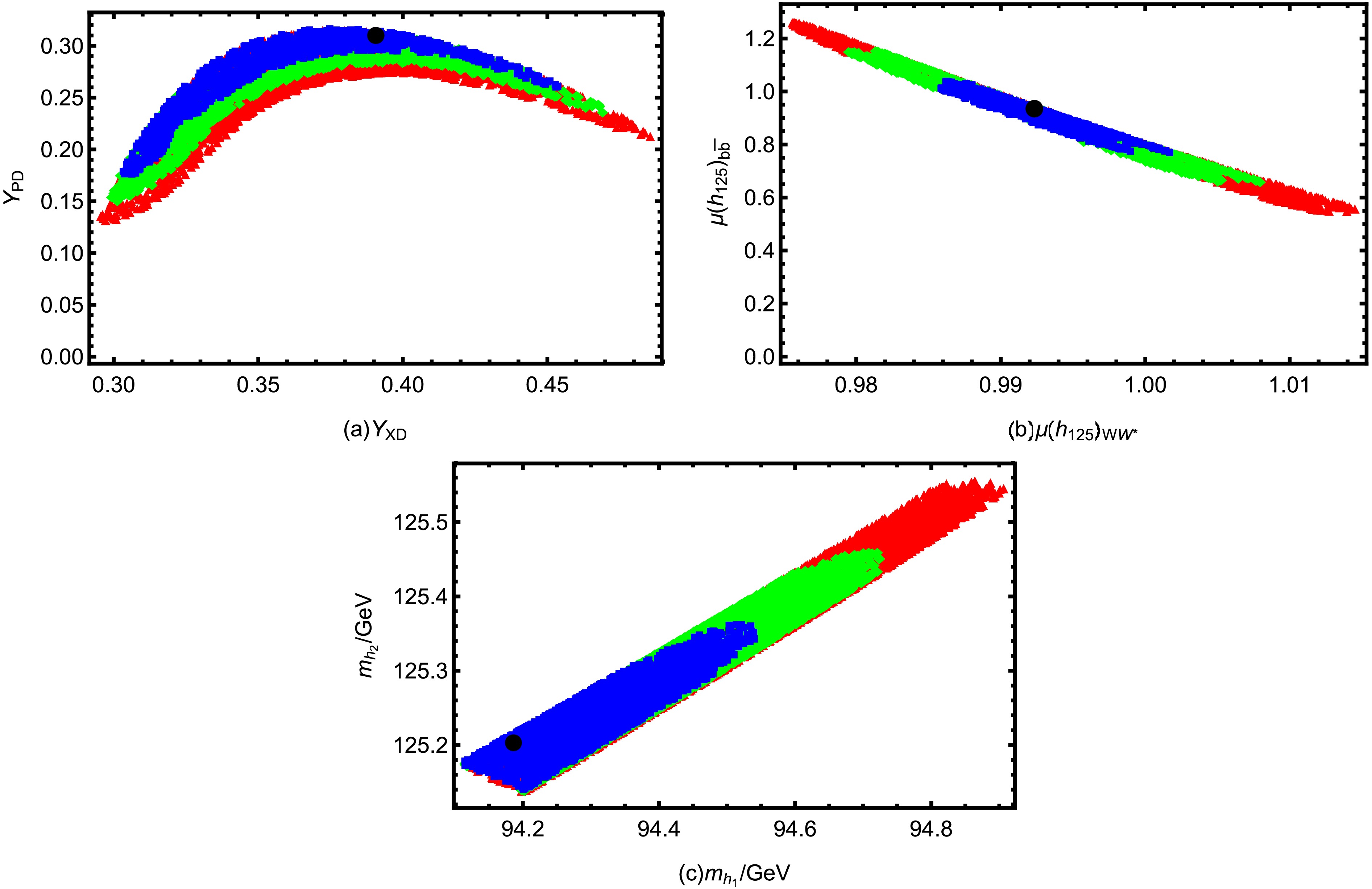
Figure 1. (color online) The symbols denote the
$ \chi^2 $ confidence regions as follows: • denotes the best-fit point ($ \chi^2_{\rm{min}} = 3.83 $ ); ■ denotes the$ 1\sigma $ region ($ \chi^2 \leq 6.13 $ ); ♦ denotes the$ 1 $ -$ 2\sigma $ region ($ 6.13 \lt \chi^2 \leq 10.01 $ ); and ▲ denotes the$ 2 $ -$ 3\sigma $ region ($ 10.01 \lt \chi^2 \leq 15.66 $ ).As shown in Fig. 1(a), the allowed region in the
$ (Y_{XD},Y_{PD}) $ plane forms a narrow arc-shaped band, indicating a strong correlation between the two parameters. The viable points cluster in the ranges$ Y_{XD}\sim0.30-0.47 $ and$ Y_{PD}\sim0.15-0.30 $ , with the best-fit point at approximately (0.391, 0.310). The$ 1\sigma $ (■) region lies along the outer side of the arc and is somewhat shorter, while the$ 2\sigma $ (♦) and$ 3\sigma $ (▲) regions lie inward along the same trajectory and cover progressively larger portions. Within this correlated region, smaller$ \chi^2 $ values are more frequently found at relatively larger$ Y_{PD} $ , indicating a mild preference for larger$ Y_{PD} $ .In Fig. 1(b), the points form a narrow, descending band, revealing a clear anticorrelation between
$ \mu(h_{125})_{WW^*} $ and$ \mu(h_{125})_{b\bar b} $ . The lowest-$ \chi^2 $ points are shown as ■, transitioning to ♦ and then ▲ toward the band edges. This pattern implies that when one signal strength increases, the other must decrease accordingly. As a result, they cannot vary independently and are strongly constrained by precise Higgs measurements.In Fig. 1(c), a diagonal band of allowed points is observed, indicating a clear positive correlation between the two Higgs masses. As
$ m_{h_1} $ increases from about 94.1 to 94.9 GeV,$ m_{h_2} $ rises in parallel from roughly 125.1 to 125.6 GeV. The band is relatively broad, suggesting that both masses can shift together within a finite range while remaining consistent with the constraints. The best-fit point, indicated by the black dot, is located at approximately$ m_{h_1}=94.19\; {\rm{GeV}} $ and$ m_{h_2}=125.20\; {\rm{GeV}} $ , a result that is particularly significant, as it simultaneously aligns with the 95 GeV scalar excess and the observed 125 GeV Higgs boson.The parameter
$ Y_{XE} $ governs the mixing between the vector-like lepton and the tau lepton, while$ Y_{PE} $ primarily determines the mass of the vector-like lepton. Figure 2 presents the$ \chi^2 $ distribution obtained from a scan over$ Y_{XE} $ and$ Y_{PE} $ within$ 0<Y_{XE}<0.8 $ and$ 0.1<Y_{PE}<0.6 $ , using the benchmark parameters$ g_X=0.41 $ ,$ g_{YX}=-0.1 $ ,$ Y_{PU}= 0.41 $ ,$ Y_{XU}=0.49 $ ,$ Y_{PD}=0.3 $ ,$ Y_{XD}=0.41 $ ,$ v_S=1600\rm\; GeV $ , and$ v_P=1900\; {\rm{GeV}} $ . The best-fit point ($ \chi^2_{\rm{min}}=4.0 $ , •) is indicated, and the$ 1\sigma $ (■),$ 1 $ -$ 2\sigma $ (♦), and$ 2 $ -$ 3\sigma $ (▲) regions highlight the parameter space favored by the fit.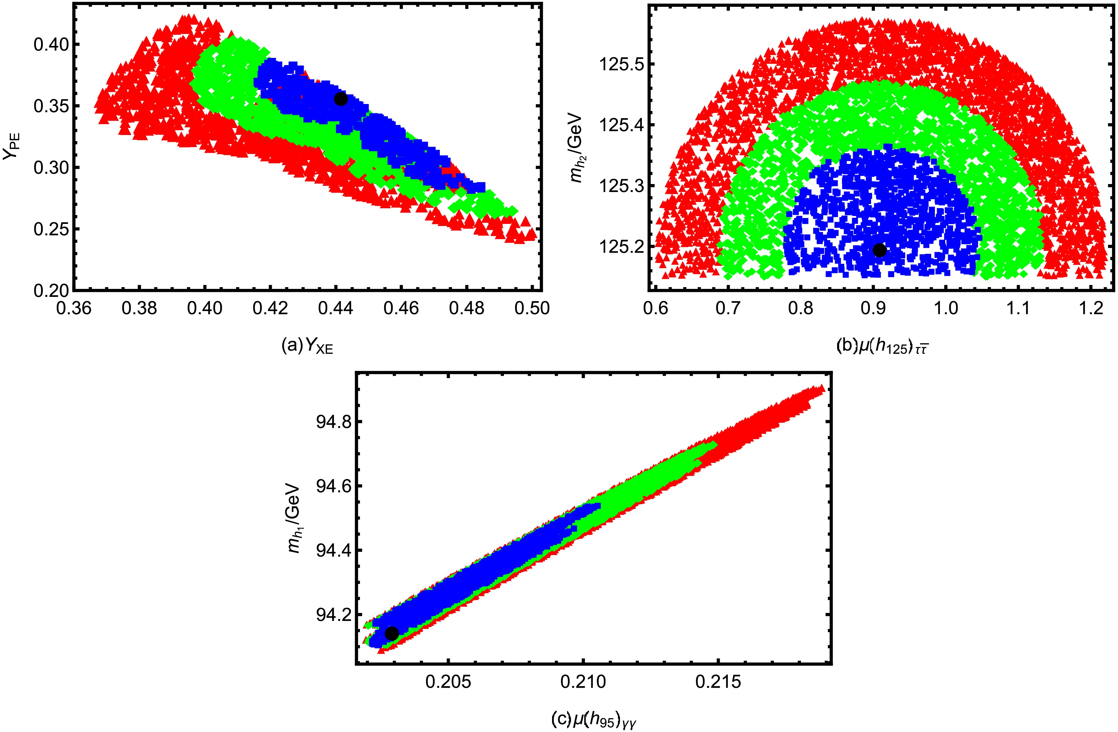
Figure 2. (color online) The symbols indicate the
$ \chi^2 $ confidence regions: • marks the best-fit point ($ \chi^2_{\rm{min}} = 4.0 $ ); ■ denotes the$ 1\sigma $ region ($ \chi^2 \leq 6.3 $ ); ♦ indicates the$ 1 $ -$ 2\sigma $ region ($ 6.3 \lt \chi^2 \leq 10.18 $ ); and ▲ corresponds to the$ 2 $ -$ 3\sigma $ region ($ 10.18 \lt \chi^2 \leq 15.83 $ ).In Fig. 2(a), the allowed parameter space forms a tilted, wedge-like strip extending from the upper left to the lower right of the (
$ Y_{XE} $ ,$ Y_{PE} $ ) plane, indicating a clear inverse correlation between the two couplings. The best-fit point lies within the compact 1σ region, while the 2σ and 3σ regions expand outward along the same orientation. This stratified pattern suggests that only correlated variations in$ Y_{XE} $ and$ Y_{PE} $ are compatible with the Higgs signal strength measurements, thereby imposing stringent constraints on the Yukawa structure in the lepton sector.In Fig. 2(b), we map the viable points in the plane spanned by the
$ \tau\bar\tau $ signal strength of$ h_{125} $ and the mass of the 125 GeV Higgs boson. The results exhibit a series of nested, semicircular layers centered on$ m_{h_2}\simeq 125.2\; \text{GeV} $ , reflecting the strong experimental preference for a Higgs-boson mass consistent with that of the SM-like Higgs boson. The$ 1\sigma $ region (■) is tightly concentrated near this central value, while the$ 2\sigma $ (♦) and$ 3\sigma $ (▲) regions form successive shells that extend outward, indicating a gradual deterioration of the fit quality as the mass departs from the preferred point. The best-fit point, marked by the black dot at$ (\mu(h_{125})_{\tau\bar\tau}, m_{h_2}) \simeq (0.91,125.19\; \text{GeV}) $ , lies extremely close to the PDG world average of$ m_{h_2}=125.20\pm 0.11\; \text{GeV} $ , demonstrating excellent agreement between the model prediction and current Higgs measurements. This pattern indicates that, with the Higgs mass fixed near its measured value, the$ \tau\bar\tau $ signal strength can vary only within a very narrow range because of strong experimental constraints.In Fig. 2(c), we show the correlation between the diphoton signal strength of the 95 GeV scalar,
$ \mu(h_{95})_{\gamma\gamma} $ , and its mass$ m_{h_1} $ . The distribution of points forms an inclined band, indicating a positive correlation:$ m_{h_1} $ increases from approximately 94.1 GeV to 95.0 GeV as$ \mu(h_{95})_{\gamma\gamma} $ increases. The global best-fit point is located at the lower boundary of this region. The symbols and their colors represent the CL, with ■ denoting the most favored region, followed by ♦ and then ▲. This correlation reflects intrinsic model constraints that link the diphoton rate and the mass of the 95 GeV scalar.Similarly, in the up-type quark sector, the parameters
$ Y_{XU} $ and$ Y_{PU} $ characterize the Yukawa interactions responsible for the coupling between the SM top quark and a vector-like fermion. They determine the strength of this interaction, thereby influencing the structure of the up-type quark mass matrix and the mixing pattern in the extended quark sector. Both parameters are included as scan variables in the numerical analysis. In Fig. 3, with$ g_X=0.41 $ ,$ g_{YX}=-0.1 $ ,$ Y_{XE}=0.46 $ ,$ Y_{PE}=0.32 $ ,$ Y_{XD}=0.41 $ ,$ Y_{PD}=0.3 $ ,$ v_S=1600\; {\rm{GeV}} $ , and$ v_P=1900\; {\rm{GeV}} $ fixed, we perform a parameter scan over$ Y_{XU} $ and$ Y_{PU} $ across$ 0<Y_{XU}<0.8 $ and$ 0.1<Y_{PU}<0.6 $ . The best-fit point is found at$ \chi^2_{\rm{min}} = 3.36 $ , while the surrounding regions correspond approximately to the$ 1\sigma $ ($ \chi^2 \leq 5.66 $ ),$ 1 $ -$ 2\sigma $ ($ 5.66 \lt \chi^2 \leq 9.54 $ ), and$ 2 $ -$ 3\sigma $ ($ 9.54 \lt \chi^2 \leq 15.19 $ ) confidence levels.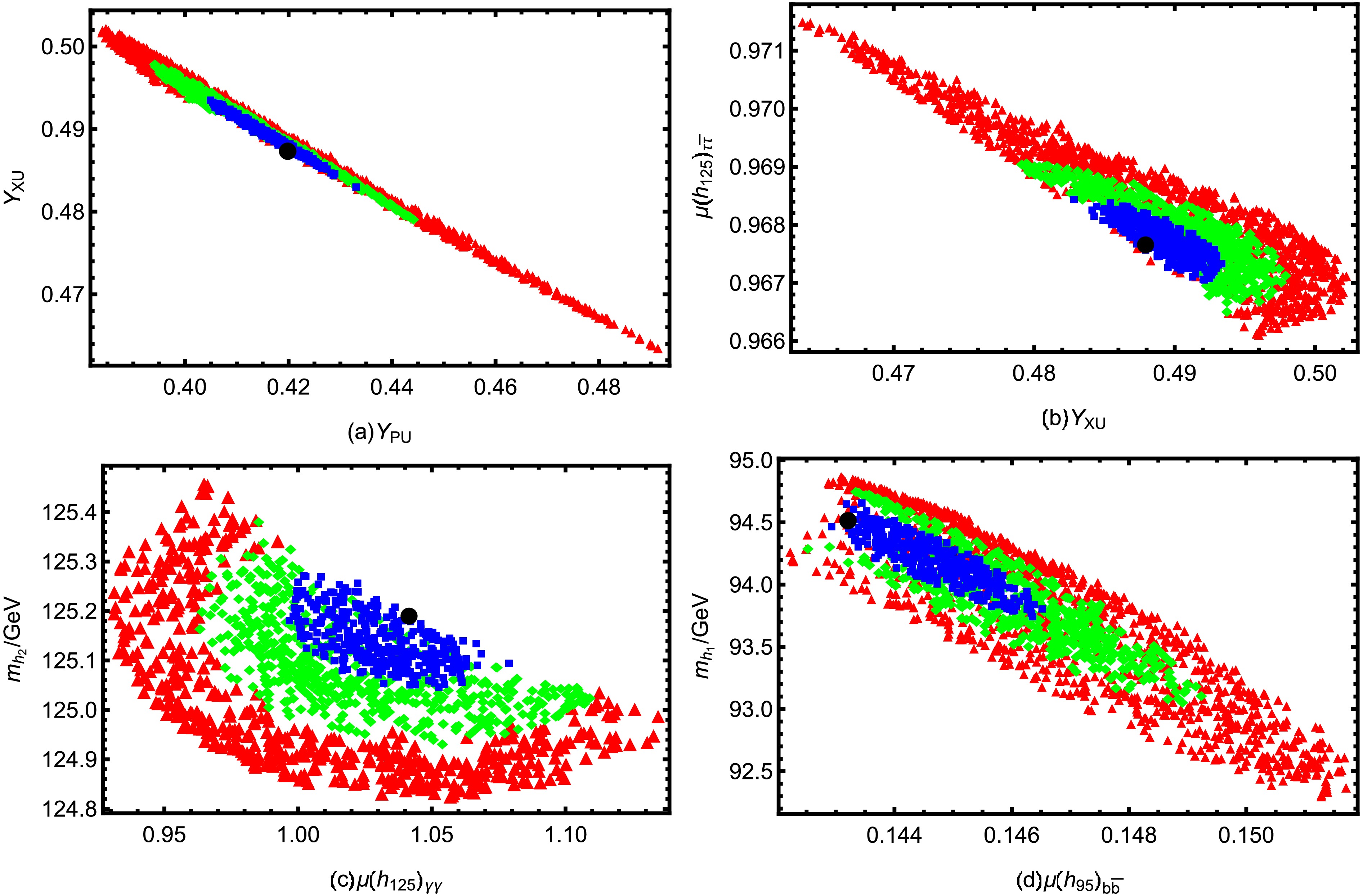
Figure 3. (color online) The symbols denote the
$ \chi^2 $ confidence regions as follows: • denotes the best-fit point ($ \chi^2_{\rm{min}} = 3.36 $ ); ■ denotes the$ 1\sigma $ region ($ \chi^2 \leq 5.66 $ ); ♦ denotes the$ 1 $ -$ 2\sigma $ region ($ 5.66 \lt \chi^2 \leq 9.54 $ ); and ▲ denotes the$ 2 $ -$ 3\sigma $ region ($ 9.54 \lt \chi^2 \leq 15.19 $ ).Figure 3(a) displays the fitted parameter distribution in the
$ (Y_{PU},Y_{XU}) $ plane. The points align along a well-defined descending strip, reflecting a compensating relation between the two couplings. The global best-fit point, marked by the black dot at$ (Y_{PU},Y_{XU})\simeq(0.420,0.487) $ , lies within the compact$ 1\sigma $ region, which is successively enclosed by the broader$ 2\sigma $ and$ 3\sigma $ confidence regions. This nested structure highlights the statistical hierarchy of the fit and demonstrates that Higgs observables can be satisfied only through a tightly correlated adjustment of$ Y_{PU} $ and$ Y_{XU} $ .Figure 3(b) shows the correlation between
$ Y_{XU} $ and$ \mu(h_{125})_{\tau\bar\tau} $ . Compared with Fig. 3(a), the distribution here is noticeably broader, with the outer regions extending into a long descending tail. The best-fit point lies near the center of the innermost domain, and any deviation from this point quickly worsens the fit. This pattern indicates that, although some flexibility exists, the$ \tau\bar\tau $ signal strength remains tightly correlated with$ Y_{XU} $ .Figure 3(c) presents the distribution of points in the plane of the
$ h_{125} $ diphoton signal strength versus its mass ($ \mu(h_{125})_{\gamma\gamma} $ ,$ m_{h_2} $ ). The points trace a tilted, semicircular arc:$ m_{h_2} $ is constrained within a narrow range of 124.8-125.4 GeV, while$ \mu(h_{125})_{\gamma\gamma} $ varies close to the SM expectation, spanning 0.95-1.10. It reveals a compact ■ core, successively surrounded by ♦ and ▲ layers that form nested semicircular envelopes, with the outer layer spanning the widest arc. The global best-fit point at ($ \mu(h{_{125}})_{\gamma\gamma}, m_{h_2}) \simeq (1.04,125.19\; \mathrm{GeV}) $ lies well inside the core. A mild anticorrelation emerges along the arc, with$ m_{h_2} $ decreasing slightly as$ \mu(h_{125})_{\gamma\gamma} $ increases, indicating constrained joint variations rather than independent scatter.In Fig. 3(d), the allowed points cluster into a diagonal band extending from the upper-left to the lower-right of the (
$ \mu(h_{95})_{b\bar b} $ ,$ m_{h_1} $ ) plane. The strip exhibits a compact ■ core is enclosed by ♦ and then ▲ regions, forming a slender corridor of viable points. A clear anticorrelation is observed: larger values of$ \mu(h_{95})_{b\bar b} $ correspond to smaller$ m_{h_1} $ , indicating that the two observables are tightly constrained by the fit. The best-fit point, ($ \mu(h_{95})_{b\bar b}, m_{h_1}) \simeq (0.143,94.51\; \mathrm{GeV}) $ , lies near the upper boundary of the ■ core, highlighting a preference for a slightly heavier$ h_1 $ mass accompanied by a reduced$ b\bar b $ signal strength.In the
$ U(1)_X $ VLFM,$ v_S $ and$ v_P $ denote the VEVs of the singlet scalars S and$ \phi_P $ , respectively. These VEVs break the extra$ U(1)_X $ gauge symmetry and generate masses for the new gauge boson$ Z' $ as well as the vector-like fermions through their Yukawa interactions. They also play an important role in determining the scalar mass spectrum. Therefore, we take$ v_S $ and$ v_P $ as key parameters in our numerical analysis. In Fig. 4, we perform an extended scan over the scalar VEVs,$ 1200\; {\rm{GeV}} \lt v_S \lt 2500\; {\rm{GeV}} $ and$ 1600\; {\rm{GeV}} \lt v_P \lt 2800\; {\rm{GeV}} $ , while keeping$ g_X=0.41 $ ,$ g_{YX}=-0.1 $ ,$ Y_{XE}=0.46 $ ,$ Y_{PE}=0.32 $ ,$ Y_{XD}=0.41 $ ,$ Y_{PD}=0.3 $ ,$ Y_{XU}=0.49 $ , and$ Y_{PU}=0.41 $ fixed. The resulting$ \chi^2 $ distribution is shown, with the best-fit point at$ \chi^2_{\rm{min}}=4.39 $ (•) and the$ 1\sigma $ ,$ 1 $ -$ 2\sigma $ , and$ 2 $ -$ 3\sigma $ confidence regions indicated by ■, ♦, and ▲, respectively.
Figure 4. (color online) The symbols denote the
$ \chi^2 $ confidence regions: • marks the best-fit point ($ \chi^2_{\rm{min}} = 4.39 $ ), ■ the$ 1\sigma $ region ($ \chi^2 \leq 6.69 $ ), ♦ the$ 1 $ -$ 2\sigma $ region ($ 6.69 \lt \chi^2 \leq 10.57 $ ), and ▲ the$ 2 $ -$ 3\sigma $ region ($ 10.57 \lt \chi^2 \leq 16.22 $ ).Figure 4(a) displays the viable region in the
$ (v_S, v_P) $ plane. The points align along a narrow diagonal band, revealing a strong positive correlation between the two VEVs. The distribution is coded by$ \chi^2 $ using both color and shape, with a compact ■ core, surrounded by ♦, and ▲ outer layers, corresponding to increasing$ \chi^2 $ values. The best-fit point,$ (v_S, v_P)\simeq(1601.8,1915.2\; \mathrm{GeV}) $ , lies near the center of the innermost region, representing the most statistically favored vacuum configuration.Figure 4(b) depicts the correlation between the Higgs signal strength in the
$ ZZ^* $ channel and the mass of the lightest scalar,$ m_{h_1} $ . The points trace a curved band with a negative slope, in which larger$ \mu(h_{125})_{ZZ^*} $ values correspond to smaller$ m_{h_1} $ . The best-fit point,$ (\mu(h_{125})_{ZZ^*}, m_{h_1}) \simeq (1.00, 94.02\; \mathrm{GeV}) $ , lies near the densest region. The point distribution reflects the fit quality: points near the center of the band agree better with the data, whereas those farther away correspond to poorer fits along the same trend. Even small deviations of$ \mu(h_{125})_{ZZ^*} $ from unity induce noticeable shifts in$ m_{h_1} $ , indicating that the light-scalar sector is highly sensitive to precision Higgs measurements.Figure 4(c) shows the distribution of points in the
$ (\mu(h_{95})_{\gamma\gamma}, m_{h_2}) $ plane. The values of$ \mu(h_{95})_{\gamma\gamma} $ span$ 0.14 \lesssim \mu(h_{95})_{\gamma\gamma} \lesssim 0.31 $ , whereas the SM-like Higgs mass is tightly constrained to a narrow window around$ 125\; \mathrm{GeV} $ . The points exhibit a layered structure rather than a uniform spread: a compact ■ core is surrounded by a ♦ band and further enclosed by a ▲ envelope, delineating progressively less-favored regions of parameter space. The global best-fit point is located at$ (\mu(h_{95})_{\gamma\gamma}, m_{h_2}) \simeq (0.152, 125.21\; \mathrm{GeV}) $ , lying within the innermost region. This pattern highlights that the Higgs mass is tightly constrained, in contrast to the greater flexibility of the diphoton rate.In the
$ U(1)_X $ VLFM,$ g_X $ denotes the gauge coupling of the additional$ U(1)_X $ symmetry, while the parameter$ g_{YX} $ quantifies the gauge mixing between hypercharge$ U(1)_Y $ and$ U(1)_X $ . In Fig. 5, rather than fixing$ g_X $ and$ g_{YX} $ as in the previous analyses, we allow them to vary over the broader ranges$ 0.25 \lt g_X \lt 0.7 $ and$ -0.3 \lt g_{YX} \lt 0.1 $ , keeping all other parameters fixed:$ Y_{XE}=0.46 $ ,$ Y_{PE}=0.32 $ ,$ Y_{XD}=0.41 $ ,$ Y_{PD}=0.3 $ ,$ Y_{XU}=0.49 $ ,$ Y_{PU}=0.41 $ ,$ v_S=1600 {\rm{GeV}} $ , and$ v_P=1900\; {\rm{GeV}} $ . The resulting point distribution is shown in terms of the$ \chi^2 $ values, with the best-fit point at$ \chi^2_{\rm{min}}=4.41 $ (indicated by •). The confidence regions are represented by ■ ($ 1\sigma $ ,$ \chi^2 \leq 6.71 $ ), ♦ ($ 1 $ -$ 2\sigma $ ,$ 6.71 \lt \chi^2 \leq 10.59 $ ), and ▲ ($ 2 $ -$ 3\sigma $ ,$ 10.59 \lt \chi^2 \leq 16.24 $ ).
Figure 5. (color online) The symbols denote the
$ \chi^2 $ confidence regions: • marks the best-fit point ($ \chi^2_{\rm{min}} = 4.41 $ ); ■ the$ 1\sigma $ region ($ \chi^2 \leq 6.71 $ ); ♦ the$ 1 $ -$ 2\sigma $ region ($ 6.71 \lt \chi^2 \leq 10.59 $ ); and ▲ the$ 2 $ -$ 3\sigma $ region ($ 10.59 \lt \chi^2 \leq 16.24 $ ).Figure 5(a) presents the correlation between
$ g_X $ and the Higgs signal strength$ \mu(h_{125})_{\tau\tau} $ . The scanned points form a positively correlated band, indicating that larger$ g_X $ generally enhances$ \mu(h_{125})_{\tau\tau} $ . Fit quality is encoded by color and shape: the most-favored points (■) cluster in the lower-left region of the band, while less-favored points (♦ and ▲) lie farther along the same trend.Figure 5(b) plots
$ g_{YX} $ versus$ \mu(h_{125})_{ZZ^*} $ . The points lie within a horizontally elongated band with a slight negative slope: those in the$ 1\sigma $ region (■) are concentrated at the lower edge of the band, while the$ 2\sigma $ (♦) and$ 3\sigma $ (▲) regions extend upward. This pattern highlights the sensitivity of$ \mu(h_{125})_{ZZ^*} $ to gauge mixing effects.Figure 5(c) shows the relationship between the masses of the two CP-even Higgs bosons,
$ m_{h_1} $ and$ m_{h_2} $ . The points are confined to a narrow diagonal strip, consistent with a scenario in which one scalar has a mass near 95 GeV, aligning with the potential excess, while the other corresponds to the observed Higgs boson at 125 GeV. The fit quality is indicated by a color gradient along the diagonal: the blue area encompasses the global best-fit point at ($ m_{h_1} $ ,$ m_{h_2} $ )$ \simeq $ (94.17,125.20) GeV, suboptimal points appear in green, and poorer fits in red. This blue-to-red gradient clearly illustrates the variation in$ \chi^2 $ and underscores the excellent agreement of the model predictions with the Higgs data.In the parameter ranges corresponding to Fig. 4,
$ v_S = 1200-2500 $ GeV and$ v_P = 1600-2800 $ GeV; in Fig. 5,$ g_{YX} = -0.3-0.1 $ and$ g_X = 0.25-0.7 $ . Since$ \dfrac{g_{YX}^2}{g_X^2}<1 $ , the correction is dominated by the suppression factor$ \dfrac{v^2}{16 v_P^2 + 4 v_S^2} $ . For the representative parameter choices used in Figs. 4 and 5 ($ g_{YX}=-0.1,\; g_X=0.41,\; v=246{\; {\rm{GeV}}}, v_S=1600 {\; {\rm{GeV}}},\; v_P=1900 \; {{\rm{GeV}}} $ ), the correction is at the$ 10^{-5} $ level. -
In our numerical analysis, we assume that the lightest CP-even Higgs boson has a mass around
$ 95\; {\rm{GeV}} $ , while the next-to-lightest CP-even Higgs boson is identified with the SM-like state at$ 125\; {\rm{GeV}} $ . The masses and associated signal strengths of these states are then discussed within the$ U(1)_X $ VLFM framework, subject to the following phenomenological constraints:1. The second-lightest CP-even Higgs boson
$ h_{2} $ is taken to be the observed Higgs boson, with mass$ m_{h_{2}} = 125.20 \pm 0.11\; {\rm{GeV}} $ as reported by the PDG [4].2. The third-generation fermion masses are required to match their SM values after mixing with the vector-like fermions [4].
3. For the vector-like fermions in the
$ U(1)_X $ VLFM, we take them to be at the TeV scale [62−64].4. Motivated by previous analyses of
$ U(1)_X $ extensions with vector-like fermions, we allow the$ Z' $ mass to be at the TeV scale in our numerical study, as such values have been shown to be phenomenologically viable in Refs. [65, 66].These constraints are imposed in the parameter scan to ensure consistency with current experimental data. For the subsequent numerical analysis, we adopt the following representative benchmark scenario:
$ \begin{aligned}[b]& Q_a = 1,\; \; Q_b = 1,\; \; Y_{XN} = 0.4,\; \; Y_{PN} = 0.4,\; \; \lambda_H = -0.12,\\& \lambda_P =-0.003,\; \; \lambda_X = -0.05,\; \; \lambda_{HP} = -0.01,\; \; \lambda_{HX} = -0.03,\\& \lambda_{PX} = -0.01,\; \; Y_{u_3} = 1.51Y_t,\; \; Y_{d_3}=1.54Y_b,\; \; Y_{e_3} = 1.5Y_\tau. \end{aligned} $
(62) Here
$ Y_t $ ,$ Y_b $ , and$ Y_\tau $ denote the Yukawa couplings of the top quark, bottom quark, and tau lepton, respectively, defined as$ Y_t = \sqrt{2} m_t/v $ ,$ Y_b = \sqrt{2} m_b/v $ , and$ Y_\tau = \sqrt{2} m_\tau/v $ .The benchmark points in this work are not chosen arbitrarily but are determined by the model structure and experimental constraints. In the
$ U(1)_X $ VLFM model considered in this paper, the CP-even neutral scalar sector is described by a$ 3\times3 $ mass matrix, and it must simultaneously accommodate a$ 125.20 \pm 0.11\; {\rm{GeV}} $ scalar consistent with the SM Higgs and a light scalar around 95 GeV [4]. These two mass conditions impose stringent constraints on the parameter space: the parameters directly related to the scalar masses are confined to relatively narrow intervals, thereby significantly reducing their freedom.On this basis, we further combine the Higgs signal strength measurements at 125 GeV and the excess around 95 GeV and perform a joint
$ \chi^2 $ fit across multiple decay channels. This procedure imposes additional experimental constraints on the parameter space, further restricting the region compatible with all observations.In contrast, parameters that are not directly related to the masses of these two scalars but mainly affect their decay properties have relatively broader allowed ranges and retain some degree of variability. Although the benchmark point we present corresponds to the optimal fit obtained from the
$ \chi^2 $ analysis, these parameters can still vary within certain ranges while maintaining a good description of the experimental data.The benchmark point given in this work corresponds to the best-fit point obtained from the
$ \chi^2 $ analysis. Therefore, the apparent concentration of these parameter values mainly originates from the compression of the parameter space required to simultaneously satisfy the 95 GeV and 125 GeV experimental constraints, rather than from any ad hoc choice. In addition, the constrained parameter ranges are consistent with the typical physical scales expected in the model.Using this benchmark, the
$ U(1)_X $ VLFM predictions are tested against Higgs data via a$ \chi^2 $ analysis, with points having$ \chi^2 $ within the$ 3\sigma $ range of the best-fit value considered favored. The$ \chi^2 $ is defined as$ \begin{aligned}[b] \chi^2 =\;&\sum\limits_i \left(\frac{\mu^{th}_i - \mu^{exp}_i}{\delta_i}\right)^2 = \Big(\frac{m^{th}_{h(125)} - m^{exp}_{h(125)}}{\delta_{m_{h}(125)}}\Big)^2 \\&+ \Big(\frac{\mu^{th}_{b\bar b(95)} - \mu^{exp}_{b\bar b(95)}}{\delta_{\mu^{95}_{b\bar b}}}\Big)^2 + \Big(\frac{\mu^{th}_{\gamma\gamma(95)} - \mu^{exp}_{\gamma\gamma(95)}}{\delta_{\mu^{95}_{\gamma \gamma}}}\Big)^2 \\ & + \Big(\frac{\mu^{th}_{\gamma\gamma(125)} - \mu^{exp}_{\gamma\gamma(125)}}{\delta_{\mu^{125}_{\gamma \gamma}}}\Big)^2 + \Big(\frac{\mu^{th}_{b\bar b(125)} - \mu^{exp}_{b\bar b(125)}}{\delta_{\mu^{125}_{b\bar b}}}\Big)^2 \\&+ \Big(\frac{\mu^{th}_{ZZ^*(125)} - \mu^{exp}_{ZZ^*(125)}}{\delta_{\mu^{125}_{ZZ^*}}}\Big)^2 + \Big(\frac{\mu^{th}_{WW^*(125)} - \mu^{exp}_{WW^*(125)}}{\delta_{\mu^{125}_{WW^*}}}\Big)^2 \\&+ \Big(\frac{\mu^{th}_{\tau\bar\tau(125)} - \mu^{exp}_{\tau\bar\tau(125)}}{\delta_{\mu^{125}_{\tau\bar\tau}}}\Big)^2, \end{aligned} $
(63) Here,
$ \mu^{exp}_i $ denotes the experimental value of the corresponding observable, while$ \mu^{th}_i $ represents its theoretical prediction. The term$ \delta_i $ stands for the total uncertainty on the observable, including statistical and systematic experimental errors as well as theoretical uncertainties. The fit includes the$ 125\; \text{GeV} $ Higgs boson mass, its signal strengths in the$ \gamma\gamma $ ,$ ZZ^* $ ,$ WW^* $ ,$ b\bar b $ , and$ \tau\bar\tau $ channels, and the potential excess at$ 95\; \text{GeV} $ in the$ \gamma\gamma $ and$ b\bar b $ final states. By accounting for multiple experimental constraints from diverse physical processes, the parameter space obtained through the$ \chi^2 $ analysis is more tightly constrained and reliable.The parameters
$ Y_{XD} $ and$ Y_{PD} $ represent the Yukawa couplings that link the SM-like and vector-like down-type quarks. Specifically,$ Y_{XD} $ couples the SM right-handed down quarks ($ d_R $ ) to the vector-like left-handed components ($ d_{XL} $ ), while$ Y_{PD} $ couples the left- and right-handed components of the vector-like quarks ($ d_{XL} $ and$ d_{XR} $ ). After the singlet scalars S and$ \phi_P $ acquire vacuum expectation values (VEVs)$ v_S $ and$ v_P $ , these couplings contribute to the mass-mixing structure of the extended quark sector, affecting both the quark masses and their interactions with the Higgs and$ Z' $ bosons. We therefore treat them as scan parameters in our analysis. Fig. 1 shows the results of the parameter scan with the benchmark set$ g_X=0.41 $ ,$ g_{YX}=-0.1 $ ,$ Y_{PU}=0.41 $ ,$ Y_{XU}=0.49 $ ,$ Y_{PE}=0.32 $ ,$ Y_{XE}=0.46 $ ,$ v_S=1600\; {\rm{GeV}} $ , and$ v_P=1900\; {\rm{GeV}} $ . The scan ranges are$ 0<Y_{XD}<0.8 $ and$ 0.1<Y_{PD}<0.6 $ . The best-fit point ($ \chi^2_{\rm{min}}=3.83 $ ) is indicated by a black dot, and the$ 1\sigma $ ,$ 2\sigma $ , and$ 3\sigma $ confidence regions are represented by ■, ♦, and ▲, respectively.
Figure 1. The symbols denote the
$ \chi^2 $ confidence regions as follows: • denotes the best-fit point ($ \chi^2_{\rm{min}} = 3.83 $ ); ■ denotes the$ 1\sigma $ region ($ \chi^2 \leq 6.13 $ ); ♦ denotes the$ 1 $ -$ 2\sigma $ region ($ 6.13 \lt \chi^2 \leq 10.01 $ ); and ▲ denotes the$ 2 $ -$ 3\sigma $ region ($ 10.01 \lt \chi^2 \leq 15.66 $ ).As shown in Fig. 1(a), the allowed region in the
$ (Y_{XD},Y_{PD}) $ plane forms a narrow arc-shaped band, indicating a strong correlation between the two parameters. The viable points cluster in the ranges$ Y_{XD}\sim0.30\text{-}0.47 $ and$ Y_{PD}\sim0.15\text{-}0.30 $ , with the best-fit point at approximately (0.391, 0.310). The$ 1\sigma $ (■) region lies along the outer side of the arc and is somewhat shorter, while the$ 2\sigma $ (♦) and$ 3\sigma $ (▲) regions lie inward along the same trajectory and cover progressively larger portions. Within this correlated region, smaller$ \chi^2 $ values are more frequently found at relatively larger$ Y_{PD} $ , indicating a mild preference for larger$ Y_{PD} $ .In Fig. 1(b), the points form a narrow, descending band, revealing a clear anticorrelation between
$ \mu(h_{125})_{WW^*} $ and$ \mu(h_{125})_{b\bar b} $ . The lowest-$ \chi^2 $ points are shown as ■, transitioning to ♦ and then ▲ toward the band edges. This pattern implies that when one signal strength increases, the other must decrease accordingly. As a result, they cannot vary independently and are strongly constrained by precise Higgs measurements.In Fig. 1(c), a diagonal band of allowed points is observed, indicating a clear positive correlation between the two Higgs masses. As
$ m_{h_1} $ increases from about 94.1 to 94.9 GeV,$ m_{h_2} $ rises in parallel from roughly 125.1 to 125.6 GeV. The band is relatively broad, suggesting that both masses can shift together within a finite range while remaining consistent with the constraints. The best-fit point, indicated by the black dot, is located at approximately$ m_{h_1}=94.19\; {\rm{GeV}} $ and$ m_{h_2}=125.20\; {\rm{GeV}} $ , a result that is particularly significant, as it simultaneously aligns with the 95 GeV scalar excess and the observed 125 GeV Higgs boson.The parameter
$ Y_{XE} $ governs the mixing between the vector-like lepton and the tau lepton, while$ Y_{PE} $ primarily determines the mass of the vector-like lepton. Fig. 2 presents the$ \chi^2 $ distribution obtained from a scan over$ Y_{XE} $ and$ Y_{PE} $ within$ 0<Y_{XE}<0.8 $ and$ 0.1<Y_{PE}<0.6 $ , using the benchmark parameters$ g_X=0.41 $ ,$ g_{YX}=-0.1 $ ,$ Y_{PU}=0.41 $ ,$ Y_{XU}=0.49 $ ,$ Y_{PD}=0.3 $ ,$ Y_{XD}=0.41 $ ,$ v_S=1600\rm\; GeV $ , and$ v_P=1900\; {\rm{GeV}} $ . The best-fit point ($ \chi^2_{\rm{min}}=4.0 $ , •) is indicated, and the$ 1\sigma $ (■),$ 1 $ -$ 2\sigma $ (♦), and$ 2 $ -$ 3\sigma $ (▲) regions highlight the parameter space favored by the fit.
Figure 2. The symbols indicate the
$ \chi^2 $ confidence regions: • marks the best-fit point ($ \chi^2_{\rm{min}} = 4.0 $ ); ■ denotes the$ 1\sigma $ region ($ \chi^2 \leq 6.3 $ ); ♦ indicates the$ 1 $ -$ 2\sigma $ region ($ 6.3 \lt \chi^2 \leq 10.18 $ ); and ▲ corresponds to the$ 2 $ -$ 3\sigma $ region ($ 10.18 \lt \chi^2 \leq 15.83 $ ).In Fig. 2(a), the allowed parameter space forms a tilted, wedge-like strip extending from the upper left to the lower right of the (
$ Y_{XE} $ ,$ Y_{PE} $ ) plane, indicating a clear inverse correlation between the two couplings. The best-fit point lies within the compact 1σ region, while the 2σ and 3σ regions expand outward along the same orientation. This stratified pattern suggests that only correlated variations in$ Y_{XE} $ and$ Y_{PE} $ are compatible with the Higgs signal strength measurements, thereby imposing stringent constraints on the Yukawa structure in the lepton sector.In Fig. 2(b), we map the viable points in the plane spanned by the
$ \tau\bar\tau $ signal strength of$ h_{125} $ and the mass of the 125 GeV Higgs boson. The results exhibit a series of nested, semicircular layers centered on$ m_{h_2}\simeq 125.2\; \text{GeV} $ , reflecting the strong experimental preference for a Higgs-boson mass consistent with that of the SM-like Higgs boson. The$ 1\sigma $ region (■) is tightly concentrated near this central value, while the$ 2\sigma $ (♦) and$ 3\sigma $ (▲) regions form successive shells that extend outward, indicating a gradual deterioration of the fit quality as the mass departs from the preferred point. The best-fit point, marked by the black dot at$ (\mu(h_{125})_{\tau\bar\tau}, m_{h_2}) \simeq (0.91,125.19\; \text{GeV}) $ , lies extremely close to the PDG world average of$ m_{h_2}=125.20\pm0.11\; \text{GeV} $ , demonstrating excellent agreement between the model prediction and current Higgs measurements. This pattern indicates that, with the Higgs mass fixed near its measured value, the$ \tau\bar\tau $ signal strength can vary only within a very narrow range because of strong experimental constraints.In Fig. 2(c), we show the correlation between the diphoton signal strength of the 95 GeV scalar,
$ \mu(h_{95})_{\gamma\gamma} $ , and its mass$ m_{h_1} $ . The distribution of points forms an inclined band, indicating a positive correlation:$ m_{h_1} $ increases from approximately 94.1 GeV to 95.0 GeV as$ \mu(h_{95})_{\gamma\gamma} $ increases. The global best-fit point is located at the lower boundary of this region. The symbols and their colors represent the CL, with ■ denoting the most favored region, followed by ♦ and then ▲. This correlation reflects intrinsic model constraints that link the diphoton rate and the mass of the 95 GeV scalar.Similarly, in the up-type quark sector, the parameters
$ Y_{XU} $ and$ Y_{PU} $ characterize the Yukawa interactions responsible for the coupling between the SM top quark and a vector-like fermion. They determine the strength of this interaction, thereby influencing the structure of the up-type quark mass matrix and the mixing pattern in the extended quark sector. Both parameters are included as scan variables in the numerical analysis. In Fig. 3, with$ g_X=0.41 $ ,$ g_{YX}=-0.1 $ ,$ Y_{XE}=0.46 $ ,$ Y_{PE}=0.32 $ ,$ Y_{XD}=0.41 $ ,$ Y_{PD}=0.3 $ ,$ v_S=1600\; {\rm{GeV}} $ , and$ v_P=1900\; {\rm{GeV}} $ fixed, we perform a parameter scan over$ Y_{XU} $ and$ Y_{PU} $ across$ 0<Y_{XU}<0.8 $ and$ 0.1<Y_{PU}<0.6 $ . The best-fit point is found at$ \chi^2_{\rm{min}} = 3.36 $ , while the surrounding regions correspond approximately to the$ 1\sigma $ ($ \chi^2 \leq 5.66 $ ),$ 1 $ -$ 2\sigma $ ($ 5.66 \lt \chi^2 \leq 9.54 $ ), and$ 2 $ -$ 3\sigma $ ($ 9.54 \lt \chi^2 \leq 15.19 $ ) confidence levels.
Figure 3. The symbols denote the
$ \chi^2 $ confidence regions as follows: • denotes the best-fit point ($ \chi^2_{\rm{min}} = 3.36 $ ); ■ denotes the$ 1\sigma $ region ($ \chi^2 \leq 5.66 $ ); ♦ denotes the$ 1 $ -$ 2\sigma $ region ($ 5.66 \lt \chi^2 \leq 9.54 $ ); and ▲ denotes the$ 2 $ -$ 3\sigma $ region ($ 9.54 \lt \chi^2 \leq 15.19 $ ).Fig. 3(a) displays the fitted parameter distribution in the
$ (Y_{PU},Y_{XU}) $ plane. The points align along a well-defined descending strip, reflecting a compensating relation between the two couplings. The global best-fit point, marked by the black dot at$ (Y_{PU},Y_{XU})\simeq(0.420,0.487) $ , lies within the compact$ 1\sigma $ region, which is successively enclosed by the broader$ 2\sigma $ and$ 3\sigma $ confidence regions. This nested structure highlights the statistical hierarchy of the fit and demonstrates that Higgs observables can be satisfied only through a tightly correlated adjustment of$ Y_{PU} $ and$ Y_{XU} $ .Fig. 3(b) shows the correlation between
$ Y_{XU} $ and$ \mu(h_{125})_{\tau\bar\tau} $ . Compared with Fig. 3(a), the distribution here is noticeably broader, with the outer regions extending into a long descending tail. The best-fit point lies near the center of the innermost domain, and any deviation from this point quickly worsens the fit. This pattern indicates that, although some flexibility exists, the$ \tau\bar\tau $ signal strength remains tightly correlated with$ Y_{XU} $ .Fig. 3(c) presents the distribution of points in the plane of the
$ h_{125} $ diphoton signal strength versus its mass ($ \mu(h_{125})_{\gamma\gamma} $ ,$ m_{h_2} $ ). The points trace a tilted, semicircular arc:$ m_{h_2} $ is constrained within a narrow range of 124.8-125.4 GeV, while$ \mu(h_{125})_{\gamma\gamma} $ varies close to the SM expectation, spanning 0.95-1.10. It reveals a compact ■ core, successively surrounded by ♦ and ▲ layers that form nested semicircular envelopes, with the outer layer spanning the widest arc. The global best-fit point at ($ \mu(h{_{125}})_{\gamma\gamma}, m_{h_2}) \simeq (1.04,125.19\; \mathrm{GeV}) $ lies well inside the core. A mild anticorrelation emerges along the arc, with$ m_{h_2} $ decreasing slightly as$ \mu(h_{125})_{\gamma\gamma} $ increases, indicating constrained joint variations rather than independent scatter.In Fig. 3(d), the allowed points cluster into a diagonal band extending from the upper-left to the lower-right of the (
$ \mu(h_{95})_{b\bar b} $ ,$ m_{h_1} $ ) plane. The strip exhibits a compact ■ core is enclosed by ♦ and then ▲ regions, forming a slender corridor of viable points. A clear anticorrelation is observed: larger values of$ \mu(h_{95})_{b\bar b} $ correspond to smaller$ m_{h_1} $ , indicating that the two observables are tightly constrained by the fit. The best-fit point, ($ \mu(h_{95})_{b\bar b}, m_{h_1}) \simeq (0.143,94.51\; \mathrm{GeV}) $ , lies near the upper boundary of the ■ core, highlighting a preference for a slightly heavier$ h_1 $ mass accompanied by a reduced$ b\bar b $ signal strength.In the
$ U(1)_X $ VLFM,$ v_S $ and$ v_P $ denote the VEVs of the singlet scalars S and$ \phi_P $ , respectively. These VEVs break the extra$ U(1)_X $ gauge symmetry and generate masses for the new gauge boson$ Z' $ as well as the vector-like fermions through their Yukawa interactions. They also play an important role in determining the scalar mass spectrum. Therefore, we take$ v_S $ and$ v_P $ as key parameters in our numerical analysis. In Fig. 4, we perform an extended scan over the scalar VEVs,$ 1200\; {\rm{GeV}} \lt v_S \lt 2500\; {\rm{GeV}} $ and$ 1600\; {\rm{GeV}} \lt v_P \lt 2800\; {\rm{GeV}} $ , while keeping$ g_X=0.41 $ ,$ g_{YX}=-0.1 $ ,$ Y_{XE}=0.46 $ ,$ Y_{PE}=0.32 $ ,$ Y_{XD}=0.41 $ ,$ Y_{PD}=0.3 $ ,$ Y_{XU}=0.49 $ , and$ Y_{PU}=0.41 $ fixed. The resulting$ \chi^2 $ distribution is shown, with the best-fit point at$ \chi^2_{\rm{min}}=4.39 $ (•) and the$ 1\sigma $ ,$ 1 $ -$ 2\sigma $ , and$ 2 $ -$ 3\sigma $ confidence regions indicated by ■, ♦, and ▲, respectively.Fig. 4(a) displays the viable region in the
$ (v_S, v_P) $ plane. The points align along a narrow diagonal band, revealing a strong positive correlation between the two VEVs. The distribution is coded by$ \chi^2 $ using both color and shape, with a compact ■ core, surrounded by ♦, and ▲ outer layers, corresponding to increasing$ \chi^2 $ values. The best-fit point,$ (v_S, v_P)\simeq(1601.8,1915.2\; \mathrm{GeV}) $ , lies near the center of the innermost region, representing the most statistically favored vacuum configuration.Fig. 4(b) depicts the correlation between the Higgs signal strength in the
$ ZZ^* $ channel and the mass of the lightest scalar,$ m_{h_1} $ . The points trace a curved band with a negative slope, in which larger$ \mu(h_{125})_{ZZ^*} $ values correspond to smaller$ m_{h_1} $ . The best-fit point,$ (\mu(h_{125})_{ZZ^*}, m_{h_1}) \simeq (1.00, 94.02\; \mathrm{GeV}) $ , lies near the densest region. The point distribution reflects the fit quality: points near the center of the band agree better with the data, whereas those farther away correspond to poorer fits along the same trend. Even small deviations of$ \mu(h_{125})_{ZZ^*} $ from unity induce noticeable shifts in$ m_{h_1} $ , indicating that the light-scalar sector is highly sensitive to precision Higgs measurements.Fig. 4(c) shows the distribution of points in the
$ (\mu(h_{95})_{\gamma\gamma}, m_{h_2}) $ plane. The values of$ \mu(h_{95})_{\gamma\gamma} $ span$ 0.14 \lesssim \mu(h_{95})_{\gamma\gamma} \lesssim 0.31 $ , whereas the SM-like Higgs mass is tightly constrained to a narrow window around$ 125\; \mathrm{GeV} $ . The points exhibit a layered structure rather than a uniform spread: a compact ■ core is surrounded by a ♦ band and further enclosed by a ▲ envelope, delineating progressively less-favored regions of parameter space. The global best-fit point is located at$ (\mu(h_{95})_{\gamma\gamma}, m_{h_2}) \simeq (0.152,\,125.21\; \mathrm{GeV}) $ , lying within the innermost region. This pattern highlights that the Higgs mass is tightly constrained, in contrast to the greater flexibility of the diphoton rate.In the
$ U(1)_X $ VLFM,$ g_X $ denotes the gauge coupling of the additional$ U(1)_X $ symmetry, while the parameter$ g_{YX} $ quantifies the gauge mixing between hypercharge$ U(1)_Y $ and$ U(1)_X $ . In Fig. 5, rather than fixing$ g_X $ and$ g_{YX} $ as in the previous analyses, we allow them to vary over the broader ranges$ 0.25 \lt g_X \lt 0.7 $ and$ -0.3 \lt g_{YX} \lt 0.1 $ , keeping all other parameters fixed:$ Y_{XE}=0.46 $ ,$ Y_{PE}=0.32 $ ,$ Y_{XD}=0.41 $ ,$ Y_{PD}=0.3 $ ,$ Y_{XU}=0.49 $ ,$ Y_{PU}=0.41 $ ,$ v_S=1600\; {\rm{GeV}} $ , and$ v_P=1900\; {\rm{GeV}} $ . The resulting point distribution is shown in terms of the$ \chi^2 $ values, with the best-fit point at$ \chi^2_{\rm{min}}=4.41 $ (indicated by •). The confidence regions are represented by ■ ($ 1\sigma $ ,$ \chi^2 \leq 6.71 $ ), ♦ ($ 1 $ -$ 2\sigma $ ,$ 6.71 \lt \chi^2 \leq 10.59 $ ), and ▲ ($ 2 $ -$ 3\sigma $ ,$ 10.59 \lt \chi^2 \leq 16.24 $ ).Fig. 5(a) presents the correlation between
$ g_X $ and the Higgs signal strength$ \mu(h_{125})_{\tau\tau} $ . The scanned points form a positively correlated band, indicating that larger$ g_X $ generally enhances$ \mu(h_{125})_{\tau\tau} $ . Fit quality is encoded by color and shape: the most-favored points (■) cluster in the lower-left region of the band, while less-favored points (♦ and ▲) lie farther along the same trend.Fig. 5(b) plots
$ g_{YX} $ versus$ \mu(h_{125})_{ZZ^*} $ . The points lie within a horizontally elongated band with a slight negative slope: those in the$ 1\sigma $ region (■) are concentrated at the lower edge of the band, while the$ 2\sigma $ (♦) and$ 3\sigma $ (▲) regions extend upward. This pattern highlights the sensitivity of$ \mu(h_{125})_{ZZ^*} $ to gauge mixing effects.Fig. 5(c) shows the relationship between the masses of the two CP-even Higgs bosons,
$ m_{h_1} $ and$ m_{h_2} $ . The points are confined to a narrow diagonal strip, consistent with a scenario in which one scalar has a mass near 95 GeV, aligning with the potential excess, while the other corresponds to the observed Higgs boson at 125 GeV. The fit quality is indicated by a color gradient along the diagonal: the blue area encompasses the global best-fit point at ($ m_{h_1} $ ,$ m_{h_2} $ )$ \simeq $ (94.17,125.20) GeV, suboptimal points appear in green, and poorer fits in red. This blue-to-red gradient clearly illustrates the variation in$ \chi^2 $ and underscores the excellent agreement of the model predictions with the Higgs data.In the parameter ranges corresponding to Fig. 4,
$ v_S = 1200\text{-}2500 $ GeV and$ v_P = 1600\text{-}2800 $ GeV; in Fig. 5,$ g_{YX} = -0.3\text{-}0.1 $ and$ g_X = 0.25\text{-}0.7 $ . Since$ \frac{g_{YX}^2}{g_X^2}<1 $ , the correction is dominated by the suppression factor$ \frac{v^2}{16 v_P^2 + 4 v_S^2} $ . For the representative parameter choices used in Figs. 4 and 5 ($ g_{YX}=-0.1,\; g_X=0.41,\; v=246{\; {\rm{GeV}}},\; v_S=1600{\; {\rm{GeV}}},\; v_P=1900{\; {\rm{GeV}}} $ ), the correction is at the$ 10^{-5} $ level. -
In our numerical analysis, we assume that the lightest CP-even Higgs boson has a mass around
$ 95\; {\rm{GeV}} $ , while the next-to-lightest CP-even Higgs boson is identified with the SM-like state at$ 125\; {\rm{GeV}} $ . The masses and associated signal strengths of these states are then discussed within the$ U(1)_X $ VLFM framework, subject to the following phenomenological constraints:1. The second-lightest CP-even Higgs boson
$ h_{2} $ is taken to be the observed Higgs boson, with mass$ m_{h_{2}} = 125.20 \pm 0.11\; {\rm{GeV}} $ as reported by the PDG [4].2. The third-generation fermion masses are required to match their SM values after mixing with the vector-like fermions [4].
3. For the vector-like fermions in the
$ U(1)_X $ VLFM, we take them to be at the TeV scale [67−69].4. Motivated by previous analyses of
$ U(1)_X $ extensions with vector-like fermions, we allow the$ Z' $ mass to be at the TeV scale in our numerical study, as such values have been shown to be phenomenologically viable in Refs. [70, 71].These constraints are imposed in the parameter scan to ensure consistency with current experimental data. For the subsequent numerical analysis, we adopt the following representative benchmark scenario:
$ \begin{aligned}[b]& Q_a = 1,\; \; Q_b = 1,\; \; Y_{XN} = 0.4,\; \; Y_{PN} = 0.4,\; \; \lambda_H = -0.12,\\& \lambda_P =-0.003,\; \; \lambda_X = -0.05,\; \; \lambda_{HP} = -0.01,\; \; \lambda_{HX} = -0.03,\\& \lambda_{PX} = -0.01,\; \; Y_{u_3} = 1.51Y_t,\; \; Y_{d_3}=1.54Y_b,\; \; Y_{e_3} = 1.5Y_\tau. \end{aligned} $
(62) Here
$ Y_t $ ,$ Y_b $ , and$ Y_\tau $ denote the Yukawa couplings of the top quark, bottom quark, and tau lepton, respectively, defined as$ Y_t = \sqrt{2} m_t/v $ ,$ Y_b = \sqrt{2} m_b/v $ , and$ Y_\tau = \sqrt{2} m_\tau/v $ .The benchmark points in this work are not chosen arbitrarily but are determined by the model structure and experimental constraints. In the
$ U(1)_X $ VLFM model considered in this paper, the CP-even neutral scalar sector is described by a$ 3\times3 $ mass matrix, and it must simultaneously accommodate a$ 125.20 \pm 0.11\; {\rm{GeV}} $ scalar consistent with the SM Higgs and a light scalar around 95 GeV [4]. These two mass conditions impose stringent constraints on the parameter space: the parameters directly related to the scalar masses are confined to relatively narrow intervals, thereby significantly reducing their freedom.On this basis, we further combine the Higgs signal strength measurements at 125 GeV and the excess around 95 GeV and perform a joint
$ \chi^2 $ fit across multiple decay channels. This procedure imposes additional experimental constraints on the parameter space, further restricting the region compatible with all observations.In contrast, parameters that are not directly related to the masses of these two scalars but mainly affect their decay properties have relatively broader allowed ranges and retain some degree of variability. Although the benchmark point we present corresponds to the optimal fit obtained from the
$ \chi^2 $ analysis, these parameters can still vary within certain ranges while maintaining a good description of the experimental data.The benchmark point given in this work corresponds to the best-fit point obtained from the
$ \chi^2 $ analysis. Therefore, the apparent concentration of these parameter values mainly originates from the compression of the parameter space required to simultaneously satisfy the 95 GeV and 125 GeV experimental constraints, rather than from any ad hoc choice. In addition, the constrained parameter ranges are consistent with the typical physical scales expected in the model.Using this benchmark, the
$ U(1)_X $ VLFM predictions are tested against Higgs data via a$ \chi^2 $ analysis, with points having$ \chi^2 $ within the$ 3\sigma $ range of the best-fit value considered favored. The$ \chi^2 $ is defined as$ \begin{aligned}[b] \chi^2 =\;&\sum\limits_i \left(\frac{\mu^{\rm th}_i - \mu^{\rm exp}_i}{\delta_i}\right)^2 = \Big(\frac{m^{th}_{h(125)} - m^{\rm exp}_{h(125)}}{\delta_{m_{h}(125)}}\Big)^2 \\&+ \Big(\frac{\mu^{\rm th}_{b\bar b(95)} - \mu^{\rm exp}_{b\bar b(95)}}{\delta_{\mu^{95}_{b\bar b}}}\Big)^2 + \Big(\frac{\mu^{\rm th}_{\gamma\gamma(95)} - \mu^{\rm exp}_{\gamma\gamma(95)}}{\delta_{\mu^{95}_{\gamma \gamma}}}\Big)^2 \\ & + \Big(\frac{\mu^{\rm th}_{\gamma\gamma(125)} - \mu^{\rm exp}_{\gamma\gamma(125)}}{\delta_{\mu^{125}_{\gamma \gamma}}}\Big)^2 + \Big(\frac{\mu^{\rm th}_{b\bar b(125)} - \mu^{\rm exp}_{b\bar b(125)}}{\delta_{\mu^{125}_{b\bar b}}}\Big)^2 \\&+ \Big(\frac{\mu^{\rm th}_{ZZ^*(125)} - \mu^{\rm exp}_{ZZ^*(125)}}{\delta_{\mu^{125}_{ZZ^*}}}\Big)^2 + \Big(\frac{\mu^{\rm th}_{WW^*(125)} - \mu^{\rm exp}_{WW^*(125)}}{\delta_{\mu^{125}_{WW^*}}}\Big)^2 \\&+ \Big(\frac{\mu^{\rm th}_{\tau\bar\tau(125)} - \mu^{\rm exp}_{\tau\bar\tau(125)}}{\delta_{\mu^{125}_{\tau\bar\tau}}}\Big)^2, \end{aligned} $
(63) Here,
$ \mu^{\rm exp}_i $ denotes the experimental value of the corresponding observable, while$ \mu^{\rm th}_i $ represents its theoretical prediction. The term$ \delta_i $ stands for the total uncertainty on the observable, including statistical and systematic experimental errors as well as theoretical uncertainties. The fit includes the$ 125\; \text{GeV} $ Higgs boson mass, its signal strengths in the$ \gamma\gamma $ ,$ ZZ^* $ ,$ WW^* $ ,$ b\bar b $ , and$ \tau\bar\tau $ channels, and the potential excess at$ 95\; \text{GeV} $ in the$ \gamma\gamma $ and$ b\bar b $ final states. By accounting for multiple experimental constraints from diverse physical processes, the parameter space obtained through the$ \chi^2 $ analysis is more tightly constrained and reliable.The parameters
$ Y_{XD} $ and$ Y_{PD} $ represent the Yukawa couplings that link the SM-like and vector-like down-type quarks. Specifically,$ Y_{XD} $ couples the SM right-handed down quarks ($ d_R $ ) to the vector-like left-handed components ($ d_{XL} $ ), while$ Y_{PD} $ couples the left- and right-handed components of the vector-like quarks ($ d_{XL} $ and$ d_{XR} $ ). After the singlet scalars S and$ \phi_P $ acquire vacuum expectation values (VEVs)$ v_S $ and$ v_P $ , these couplings contribute to the mass-mixing structure of the extended quark sector, affecting both the quark masses and their interactions with the Higgs and$ Z' $ bosons. We therefore treat them as scan parameters in our analysis. Figure 1 shows the results of the parameter scan with the benchmark set$ g_X=0.41 $ ,$ g_{YX}=-0.1 $ ,$ Y_{PU}=0.41 $ ,$ Y_{XU}=0.49 $ ,$ Y_{PE}=0.32 $ ,$ Y_{XE}=0.46 $ ,$ v_S=1600\; {\rm{GeV}} $ , and$ v_P=1900\; {\rm{GeV}} $ . The scan ranges are$ 0<Y_{XD}<0.8 $ and$ 0.1<Y_{PD}<0.6 $ . The best-fit point ($ \chi^2_{\rm{min}}=3.83 $ ) is indicated by a black dot, and the$ 1\sigma $ ,$ 2\sigma $ , and$ 3\sigma $ confidence regions are represented by ■, ♦, and ▲, respectively.
Figure 1. (color online) The symbols denote the
$ \chi^2 $ confidence regions as follows: • denotes the best-fit point ($ \chi^2_{\rm{min}} = 3.83 $ ); ■ denotes the$ 1\sigma $ region ($ \chi^2 \leq 6.13 $ ); ♦ denotes the$ 1 $ -$ 2\sigma $ region ($ 6.13 \lt \chi^2 \leq 10.01 $ ); and ▲ denotes the$ 2 $ -$ 3\sigma $ region ($ 10.01 \lt \chi^2 \leq 15.66 $ ).As shown in Fig. 1(a), the allowed region in the
$ (Y_{XD},Y_{PD}) $ plane forms a narrow arc-shaped band, indicating a strong correlation between the two parameters. The viable points cluster in the ranges$ Y_{XD}\sim0.30-0.47 $ and$ Y_{PD}\sim0.15-0.30 $ , with the best-fit point at approximately (0.391, 0.310). The$ 1\sigma $ (■) region lies along the outer side of the arc and is somewhat shorter, while the$ 2\sigma $ (♦) and$ 3\sigma $ (▲) regions lie inward along the same trajectory and cover progressively larger portions. Within this correlated region, smaller$ \chi^2 $ values are more frequently found at relatively larger$ Y_{PD} $ , indicating a mild preference for larger$ Y_{PD} $ .In Fig. 1(b), the points form a narrow, descending band, revealing a clear anticorrelation between
$ \mu(h_{125})_{WW^*} $ and$ \mu(h_{125})_{b\bar b} $ . The lowest-$ \chi^2 $ points are shown as ■, transitioning to ♦ and then ▲ toward the band edges. This pattern implies that when one signal strength increases, the other must decrease accordingly. As a result, they cannot vary independently and are strongly constrained by precise Higgs measurements.In Fig. 1(c), a diagonal band of allowed points is observed, indicating a clear positive correlation between the two Higgs masses. As
$ m_{h_1} $ increases from about 94.1 to 94.9 GeV,$ m_{h_2} $ rises in parallel from roughly 125.1 to 125.6 GeV. The band is relatively broad, suggesting that both masses can shift together within a finite range while remaining consistent with the constraints. The best-fit point, indicated by the black dot, is located at approximately$ m_{h_1}=94.19\; {\rm{GeV}} $ and$ m_{h_2}=125.20\; {\rm{GeV}} $ , a result that is particularly significant, as it simultaneously aligns with the 95 GeV scalar excess and the observed 125 GeV Higgs boson.The parameter
$ Y_{XE} $ governs the mixing between the vector-like lepton and the tau lepton, while$ Y_{PE} $ primarily determines the mass of the vector-like lepton. Figure 2 presents the$ \chi^2 $ distribution obtained from a scan over$ Y_{XE} $ and$ Y_{PE} $ within$ 0<Y_{XE}<0.8 $ and$ 0.1<Y_{PE}<0.6 $ , using the benchmark parameters$ g_X=0.41 $ ,$ g_{YX}=-0.1 $ ,$ Y_{PU}= 0.41 $ ,$ Y_{XU}=0.49 $ ,$ Y_{PD}=0.3 $ ,$ Y_{XD}=0.41 $ ,$ v_S=1600\rm\; GeV $ , and$ v_P=1900\; {\rm{GeV}} $ . The best-fit point ($ \chi^2_{\rm{min}}=4.0 $ , •) is indicated, and the$ 1\sigma $ (■),$ 1 $ -$ 2\sigma $ (♦), and$ 2 $ -$ 3\sigma $ (▲) regions highlight the parameter space favored by the fit.
Figure 2. (color online) The symbols indicate the
$ \chi^2 $ confidence regions: • marks the best-fit point ($ \chi^2_{\rm{min}} = 4.0 $ ); ■ denotes the$ 1\sigma $ region ($ \chi^2 \leq 6.3 $ ); ♦ indicates the$ 1 $ -$ 2\sigma $ region ($ 6.3 \lt \chi^2 \leq 10.18 $ ); and ▲ corresponds to the$ 2 $ -$ 3\sigma $ region ($ 10.18 \lt \chi^2 \leq 15.83 $ ).In Fig. 2(a), the allowed parameter space forms a tilted, wedge-like strip extending from the upper left to the lower right of the (
$ Y_{XE} $ ,$ Y_{PE} $ ) plane, indicating a clear inverse correlation between the two couplings. The best-fit point lies within the compact 1σ region, while the 2σ and 3σ regions expand outward along the same orientation. This stratified pattern suggests that only correlated variations in$ Y_{XE} $ and$ Y_{PE} $ are compatible with the Higgs signal strength measurements, thereby imposing stringent constraints on the Yukawa structure in the lepton sector.In Fig. 2(b), we map the viable points in the plane spanned by the
$ \tau\bar\tau $ signal strength of$ h_{125} $ and the mass of the 125 GeV Higgs boson. The results exhibit a series of nested, semicircular layers centered on$ m_{h_2}\simeq 125.2\; \text{GeV} $ , reflecting the strong experimental preference for a Higgs-boson mass consistent with that of the SM-like Higgs boson. The$ 1\sigma $ region (■) is tightly concentrated near this central value, while the$ 2\sigma $ (♦) and$ 3\sigma $ (▲) regions form successive shells that extend outward, indicating a gradual deterioration of the fit quality as the mass departs from the preferred point. The best-fit point, marked by the black dot at$ (\mu(h_{125})_{\tau\bar\tau}, m_{h_2}) \simeq (0.91,125.19\; \text{GeV}) $ , lies extremely close to the PDG world average of$ m_{h_2}=125.20\pm 0.11\; \text{GeV} $ , demonstrating excellent agreement between the model prediction and current Higgs measurements. This pattern indicates that, with the Higgs mass fixed near its measured value, the$ \tau\bar\tau $ signal strength can vary only within a very narrow range because of strong experimental constraints.In Fig. 2(c), we show the correlation between the diphoton signal strength of the 95 GeV scalar,
$ \mu(h_{95})_{\gamma\gamma} $ , and its mass$ m_{h_1} $ . The distribution of points forms an inclined band, indicating a positive correlation:$ m_{h_1} $ increases from approximately 94.1 GeV to 95.0 GeV as$ \mu(h_{95})_{\gamma\gamma} $ increases. The global best-fit point is located at the lower boundary of this region. The symbols and their colors represent the CL, with ■ denoting the most favored region, followed by ♦ and then ▲. This correlation reflects intrinsic model constraints that link the diphoton rate and the mass of the 95 GeV scalar.Similarly, in the up-type quark sector, the parameters
$ Y_{XU} $ and$ Y_{PU} $ characterize the Yukawa interactions responsible for the coupling between the SM top quark and a vector-like fermion. They determine the strength of this interaction, thereby influencing the structure of the up-type quark mass matrix and the mixing pattern in the extended quark sector. Both parameters are included as scan variables in the numerical analysis. In Fig. 3, with$ g_X=0.41 $ ,$ g_{YX}=-0.1 $ ,$ Y_{XE}=0.46 $ ,$ Y_{PE}=0.32 $ ,$ Y_{XD}=0.41 $ ,$ Y_{PD}=0.3 $ ,$ v_S=1600\; {\rm{GeV}} $ , and$ v_P=1900\; {\rm{GeV}} $ fixed, we perform a parameter scan over$ Y_{XU} $ and$ Y_{PU} $ across$ 0<Y_{XU}<0.8 $ and$ 0.1<Y_{PU}<0.6 $ . The best-fit point is found at$ \chi^2_{\rm{min}} = 3.36 $ , while the surrounding regions correspond approximately to the$ 1\sigma $ ($ \chi^2 \leq 5.66 $ ),$ 1 $ -$ 2\sigma $ ($ 5.66 \lt \chi^2 \leq 9.54 $ ), and$ 2 $ -$ 3\sigma $ ($ 9.54 \lt \chi^2 \leq 15.19 $ ) confidence levels.
Figure 3. (color online) The symbols denote the
$ \chi^2 $ confidence regions as follows: • denotes the best-fit point ($ \chi^2_{\rm{min}} = 3.36 $ ); ■ denotes the$ 1\sigma $ region ($ \chi^2 \leq 5.66 $ ); ♦ denotes the$ 1 $ -$ 2\sigma $ region ($ 5.66 \lt \chi^2 \leq 9.54 $ ); and ▲ denotes the$ 2 $ -$ 3\sigma $ region ($ 9.54 \lt \chi^2 \leq 15.19 $ ).Figure 3(a) displays the fitted parameter distribution in the
$ (Y_{PU},Y_{XU}) $ plane. The points align along a well-defined descending strip, reflecting a compensating relation between the two couplings. The global best-fit point, marked by the black dot at$ (Y_{PU},Y_{XU})\simeq(0.420,0.487) $ , lies within the compact$ 1\sigma $ region, which is successively enclosed by the broader$ 2\sigma $ and$ 3\sigma $ confidence regions. This nested structure highlights the statistical hierarchy of the fit and demonstrates that Higgs observables can be satisfied only through a tightly correlated adjustment of$ Y_{PU} $ and$ Y_{XU} $ .Figure 3(b) shows the correlation between
$ Y_{XU} $ and$ \mu(h_{125})_{\tau\bar\tau} $ . Compared with Fig. 3(a), the distribution here is noticeably broader, with the outer regions extending into a long descending tail. The best-fit point lies near the center of the innermost domain, and any deviation from this point quickly worsens the fit. This pattern indicates that, although some flexibility exists, the$ \tau\bar\tau $ signal strength remains tightly correlated with$ Y_{XU} $ .Figure 3(c) presents the distribution of points in the plane of the
$ h_{125} $ diphoton signal strength versus its mass ($ \mu(h_{125})_{\gamma\gamma} $ ,$ m_{h_2} $ ). The points trace a tilted, semicircular arc:$ m_{h_2} $ is constrained within a narrow range of 124.8-125.4 GeV, while$ \mu(h_{125})_{\gamma\gamma} $ varies close to the SM expectation, spanning 0.95-1.10. It reveals a compact ■ core, successively surrounded by ♦ and ▲ layers that form nested semicircular envelopes, with the outer layer spanning the widest arc. The global best-fit point at ($ \mu(h{_{125}})_{\gamma\gamma}, m_{h_2}) \simeq (1.04,125.19\; \mathrm{GeV}) $ lies well inside the core. A mild anticorrelation emerges along the arc, with$ m_{h_2} $ decreasing slightly as$ \mu(h_{125})_{\gamma\gamma} $ increases, indicating constrained joint variations rather than independent scatter.In Fig. 3(d), the allowed points cluster into a diagonal band extending from the upper-left to the lower-right of the (
$ \mu(h_{95})_{b\bar b} $ ,$ m_{h_1} $ ) plane. The strip exhibits a compact ■ core is enclosed by ♦ and then ▲ regions, forming a slender corridor of viable points. A clear anticorrelation is observed: larger values of$ \mu(h_{95})_{b\bar b} $ correspond to smaller$ m_{h_1} $ , indicating that the two observables are tightly constrained by the fit. The best-fit point, ($ \mu(h_{95})_{b\bar b}, m_{h_1}) \simeq (0.143,94.51\; \mathrm{GeV}) $ , lies near the upper boundary of the ■ core, highlighting a preference for a slightly heavier$ h_1 $ mass accompanied by a reduced$ b\bar b $ signal strength.In the
$ U(1)_X $ VLFM,$ v_S $ and$ v_P $ denote the VEVs of the singlet scalars S and$ \phi_P $ , respectively. These VEVs break the extra$ U(1)_X $ gauge symmetry and generate masses for the new gauge boson$ Z' $ as well as the vector-like fermions through their Yukawa interactions. They also play an important role in determining the scalar mass spectrum. Therefore, we take$ v_S $ and$ v_P $ as key parameters in our numerical analysis. In Fig. 4, we perform an extended scan over the scalar VEVs,$ 1200\; {\rm{GeV}} \lt v_S \lt 2500\; {\rm{GeV}} $ and$ 1600\; {\rm{GeV}} \lt v_P \lt 2800\; {\rm{GeV}} $ , while keeping$ g_X=0.41 $ ,$ g_{YX}=-0.1 $ ,$ Y_{XE}=0.46 $ ,$ Y_{PE}=0.32 $ ,$ Y_{XD}=0.41 $ ,$ Y_{PD}=0.3 $ ,$ Y_{XU}=0.49 $ , and$ Y_{PU}=0.41 $ fixed. The resulting$ \chi^2 $ distribution is shown, with the best-fit point at$ \chi^2_{\rm{min}}=4.39 $ (•) and the$ 1\sigma $ ,$ 1 $ -$ 2\sigma $ , and$ 2 $ -$ 3\sigma $ confidence regions indicated by ■, ♦, and ▲, respectively.
Figure 4. (color online) The symbols denote the
$ \chi^2 $ confidence regions: • marks the best-fit point ($ \chi^2_{\rm{min}} = 4.39 $ ), ■ the$ 1\sigma $ region ($ \chi^2 \leq 6.69 $ ), ♦ the$ 1 $ -$ 2\sigma $ region ($ 6.69 \lt \chi^2 \leq 10.57 $ ), and ▲ the$ 2 $ -$ 3\sigma $ region ($ 10.57 \lt \chi^2 \leq 16.22 $ ).Figure 4(a) displays the viable region in the
$ (v_S, v_P) $ plane. The points align along a narrow diagonal band, revealing a strong positive correlation between the two VEVs. The distribution is coded by$ \chi^2 $ using both color and shape, with a compact ■ core, surrounded by ♦, and ▲ outer layers, corresponding to increasing$ \chi^2 $ values. The best-fit point,$ (v_S, v_P)\simeq(1601.8,1915.2\; \mathrm{GeV}) $ , lies near the center of the innermost region, representing the most statistically favored vacuum configuration.Figure 4(b) depicts the correlation between the Higgs signal strength in the
$ ZZ^* $ channel and the mass of the lightest scalar,$ m_{h_1} $ . The points trace a curved band with a negative slope, in which larger$ \mu(h_{125})_{ZZ^*} $ values correspond to smaller$ m_{h_1} $ . The best-fit point,$ (\mu(h_{125})_{ZZ^*}, m_{h_1}) \simeq (1.00, 94.02\; \mathrm{GeV}) $ , lies near the densest region. The point distribution reflects the fit quality: points near the center of the band agree better with the data, whereas those farther away correspond to poorer fits along the same trend. Even small deviations of$ \mu(h_{125})_{ZZ^*} $ from unity induce noticeable shifts in$ m_{h_1} $ , indicating that the light-scalar sector is highly sensitive to precision Higgs measurements.Figure 4(c) shows the distribution of points in the
$ (\mu(h_{95})_{\gamma\gamma}, m_{h_2}) $ plane. The values of$ \mu(h_{95})_{\gamma\gamma} $ span$ 0.14 \lesssim \mu(h_{95})_{\gamma\gamma} \lesssim 0.31 $ , whereas the SM-like Higgs mass is tightly constrained to a narrow window around$ 125\; \mathrm{GeV} $ . The points exhibit a layered structure rather than a uniform spread: a compact ■ core is surrounded by a ♦ band and further enclosed by a ▲ envelope, delineating progressively less-favored regions of parameter space. The global best-fit point is located at$ (\mu(h_{95})_{\gamma\gamma}, m_{h_2}) \simeq (0.152, 125.21\; \mathrm{GeV}) $ , lying within the innermost region. This pattern highlights that the Higgs mass is tightly constrained, in contrast to the greater flexibility of the diphoton rate.In the
$ U(1)_X $ VLFM,$ g_X $ denotes the gauge coupling of the additional$ U(1)_X $ symmetry, while the parameter$ g_{YX} $ quantifies the gauge mixing between hypercharge$ U(1)_Y $ and$ U(1)_X $ . In Fig. 5, rather than fixing$ g_X $ and$ g_{YX} $ as in the previous analyses, we allow them to vary over the broader ranges$ 0.25 \lt g_X \lt 0.7 $ and$ -0.3 \lt g_{YX} \lt 0.1 $ , keeping all other parameters fixed:$ Y_{XE}=0.46 $ ,$ Y_{PE}=0.32 $ ,$ Y_{XD}=0.41 $ ,$ Y_{PD}=0.3 $ ,$ Y_{XU}=0.49 $ ,$ Y_{PU}=0.41 $ ,$ v_S=1600 {\rm{GeV}} $ , and$ v_P=1900\; {\rm{GeV}} $ . The resulting point distribution is shown in terms of the$ \chi^2 $ values, with the best-fit point at$ \chi^2_{\rm{min}}=4.41 $ (indicated by •). The confidence regions are represented by ■ ($ 1\sigma $ ,$ \chi^2 \leq 6.71 $ ), ♦ ($ 1 $ -$ 2\sigma $ ,$ 6.71 \lt \chi^2 \leq 10.59 $ ), and ▲ ($ 2 $ -$ 3\sigma $ ,$ 10.59 \lt \chi^2 \leq 16.24 $ ).
Figure 5. (color online) The symbols denote the
$ \chi^2 $ confidence regions: • marks the best-fit point ($ \chi^2_{\rm{min}} = 4.41 $ ); ■ the$ 1\sigma $ region ($ \chi^2 \leq 6.71 $ ); ♦ the$ 1 $ -$ 2\sigma $ region ($ 6.71 \lt \chi^2 \leq 10.59 $ ); and ▲ the$ 2 $ -$ 3\sigma $ region ($ 10.59 \lt \chi^2 \leq 16.24 $ ).Figure 5(a) presents the correlation between
$ g_X $ and the Higgs signal strength$ \mu(h_{125})_{\tau\tau} $ . The scanned points form a positively correlated band, indicating that larger$ g_X $ generally enhances$ \mu(h_{125})_{\tau\tau} $ . Fit quality is encoded by color and shape: the most-favored points (■) cluster in the lower-left region of the band, while less-favored points (♦ and ▲) lie farther along the same trend.Figure 5(b) plots
$ g_{YX} $ versus$ \mu(h_{125})_{ZZ^*} $ . The points lie within a horizontally elongated band with a slight negative slope: those in the$ 1\sigma $ region (■) are concentrated at the lower edge of the band, while the$ 2\sigma $ (♦) and$ 3\sigma $ (▲) regions extend upward. This pattern highlights the sensitivity of$ \mu(h_{125})_{ZZ^*} $ to gauge mixing effects.Figure 5(c) shows the relationship between the masses of the two CP-even Higgs bosons,
$ m_{h_1} $ and$ m_{h_2} $ . The points are confined to a narrow diagonal strip, consistent with a scenario in which one scalar has a mass near 95 GeV, aligning with the potential excess, while the other corresponds to the observed Higgs boson at 125 GeV. The fit quality is indicated by a color gradient along the diagonal: the blue area encompasses the global best-fit point at ($ m_{h_1} $ ,$ m_{h_2} $ )$ \simeq $ (94.17,125.20) GeV, suboptimal points appear in green, and poorer fits in red. This blue-to-red gradient clearly illustrates the variation in$ \chi^2 $ and underscores the excellent agreement of the model predictions with the Higgs data.In the parameter ranges corresponding to Fig. 4,
$ v_S = 1200-2500 $ GeV and$ v_P = 1600-2800 $ GeV; in Fig. 5,$ g_{YX} = -0.3-0.1 $ and$ g_X = 0.25-0.7 $ . Since$ \dfrac{g_{YX}^2}{g_X^2}<1 $ , the correction is dominated by the suppression factor$ \dfrac{v^2}{16 v_P^2 + 4 v_S^2} $ . For the representative parameter choices used in Figs. 4 and 5 ($ g_{YX}=-0.1,\; g_X=0.41,\; v=246{\; {\rm{GeV}}}, v_S=1600 {\; {\rm{GeV}}},\; v_P=1900 \; {{\rm{GeV}}} $ ), the correction is at the$ 10^{-5} $ level. -
In our numerical analysis, we assume that the lightest CP-even Higgs boson has a mass around
$ 95\; {\rm{GeV}} $ , while the next-to-lightest CP-even Higgs boson is identified with the SM-like state at$ 125\; {\rm{GeV}} $ . The masses and associated signal strengths of these states are then discussed within the$ U(1)_X $ VLFM framework, subject to the following phenomenological constraints:1. The second-lightest CP-even Higgs boson
$ h_{2} $ is taken to be the observed Higgs boson, with mass$ m_{h_{2}} = 125.20 \pm 0.11\; {\rm{GeV}} $ as reported by the PDG [4].2. The third-generation fermion masses are required to match their SM values after mixing with the vector-like fermions [4].
3. For the vector-like fermions in the
$ U(1)_X $ VLFM, we take them to be at the TeV scale [67−69].4. Motivated by previous analyses of
$ U(1)_X $ extensions with vector-like fermions, we allow the$ Z' $ mass to be at the TeV scale in our numerical study, as such values have been shown to be phenomenologically viable in Refs. [70, 71].These constraints are imposed in the parameter scan to ensure consistency with current experimental data. For the subsequent numerical analysis, we adopt the following representative benchmark scenario:
$ \begin{aligned}[b]& Q_a = 1,\; \; Q_b = 1,\; \; Y_{XN} = 0.4,\; \; Y_{PN} = 0.4,\; \; \lambda_H = -0.12,\\& \lambda_P =-0.003,\; \; \lambda_X = -0.05,\; \; \lambda_{HP} = -0.01,\; \; \lambda_{HX} = -0.03,\\& \lambda_{PX} = -0.01,\; \; Y_{u_3} = 1.51Y_t,\; \; Y_{d_3}=1.54Y_b,\; \; Y_{e_3} = 1.5Y_\tau. \end{aligned} $
(62) Here
$ Y_t $ ,$ Y_b $ , and$ Y_\tau $ denote the Yukawa couplings of the top quark, bottom quark, and tau lepton, respectively, defined as$ Y_t = \sqrt{2} m_t/v $ ,$ Y_b = \sqrt{2} m_b/v $ , and$ Y_\tau = \sqrt{2} m_\tau/v $ .The benchmark points in this work are not chosen arbitrarily but are determined by the model structure and experimental constraints. In the
$ U(1)_X $ VLFM model considered in this paper, the CP-even neutral scalar sector is described by a$ 3\times3 $ mass matrix, and it must simultaneously accommodate a$ 125.20 \pm 0.11\; {\rm{GeV}} $ scalar consistent with the SM Higgs and a light scalar around 95 GeV [4]. These two mass conditions impose stringent constraints on the parameter space: the parameters directly related to the scalar masses are confined to relatively narrow intervals, thereby significantly reducing their freedom.On this basis, we further combine the Higgs signal strength measurements at 125 GeV and the excess around 95 GeV and perform a joint
$ \chi^2 $ fit across multiple decay channels. This procedure imposes additional experimental constraints on the parameter space, further restricting the region compatible with all observations.In contrast, parameters that are not directly related to the masses of these two scalars but mainly affect their decay properties have relatively broader allowed ranges and retain some degree of variability. Although the benchmark point we present corresponds to the optimal fit obtained from the
$ \chi^2 $ analysis, these parameters can still vary within certain ranges while maintaining a good description of the experimental data.The benchmark point given in this work corresponds to the best-fit point obtained from the
$ \chi^2 $ analysis. Therefore, the apparent concentration of these parameter values mainly originates from the compression of the parameter space required to simultaneously satisfy the 95 GeV and 125 GeV experimental constraints, rather than from any ad hoc choice. In addition, the constrained parameter ranges are consistent with the typical physical scales expected in the model.Using this benchmark, the
$ U(1)_X $ VLFM predictions are tested against Higgs data via a$ \chi^2 $ analysis, with points having$ \chi^2 $ within the$ 3\sigma $ range of the best-fit value considered favored. The$ \chi^2 $ is defined as$ \begin{aligned}[b] \chi^2 =\;&\sum\limits_i \left(\frac{\mu^{\rm th}_i - \mu^{\rm exp}_i}{\delta_i}\right)^2 = \Big(\frac{m^{th}_{h(125)} - m^{\rm exp}_{h(125)}}{\delta_{m_{h}(125)}}\Big)^2 \\&+ \Big(\frac{\mu^{\rm th}_{b\bar b(95)} - \mu^{\rm exp}_{b\bar b(95)}}{\delta_{\mu^{95}_{b\bar b}}}\Big)^2 + \Big(\frac{\mu^{\rm th}_{\gamma\gamma(95)} - \mu^{\rm exp}_{\gamma\gamma(95)}}{\delta_{\mu^{95}_{\gamma \gamma}}}\Big)^2 \\ & + \Big(\frac{\mu^{\rm th}_{\gamma\gamma(125)} - \mu^{\rm exp}_{\gamma\gamma(125)}}{\delta_{\mu^{125}_{\gamma \gamma}}}\Big)^2 + \Big(\frac{\mu^{\rm th}_{b\bar b(125)} - \mu^{\rm exp}_{b\bar b(125)}}{\delta_{\mu^{125}_{b\bar b}}}\Big)^2 \\&+ \Big(\frac{\mu^{\rm th}_{ZZ^*(125)} - \mu^{\rm exp}_{ZZ^*(125)}}{\delta_{\mu^{125}_{ZZ^*}}}\Big)^2 + \Big(\frac{\mu^{\rm th}_{WW^*(125)} - \mu^{\rm exp}_{WW^*(125)}}{\delta_{\mu^{125}_{WW^*}}}\Big)^2 \\&+ \Big(\frac{\mu^{\rm th}_{\tau\bar\tau(125)} - \mu^{\rm exp}_{\tau\bar\tau(125)}}{\delta_{\mu^{125}_{\tau\bar\tau}}}\Big)^2, \end{aligned} $
(63) Here,
$ \mu^{\rm exp}_i $ denotes the experimental value of the corresponding observable, while$ \mu^{\rm th}_i $ represents its theoretical prediction. The term$ \delta_i $ stands for the total uncertainty on the observable, including statistical and systematic experimental errors as well as theoretical uncertainties. The fit includes the$ 125\; \text{GeV} $ Higgs boson mass, its signal strengths in the$ \gamma\gamma $ ,$ ZZ^* $ ,$ WW^* $ ,$ b\bar b $ , and$ \tau\bar\tau $ channels, and the potential excess at$ 95\; \text{GeV} $ in the$ \gamma\gamma $ and$ b\bar b $ final states. By accounting for multiple experimental constraints from diverse physical processes, the parameter space obtained through the$ \chi^2 $ analysis is more tightly constrained and reliable.The parameters
$ Y_{XD} $ and$ Y_{PD} $ represent the Yukawa couplings that link the SM-like and vector-like down-type quarks. Specifically,$ Y_{XD} $ couples the SM right-handed down quarks ($ d_R $ ) to the vector-like left-handed components ($ d_{XL} $ ), while$ Y_{PD} $ couples the left- and right-handed components of the vector-like quarks ($ d_{XL} $ and$ d_{XR} $ ). After the singlet scalars S and$ \phi_P $ acquire vacuum expectation values (VEVs)$ v_S $ and$ v_P $ , these couplings contribute to the mass-mixing structure of the extended quark sector, affecting both the quark masses and their interactions with the Higgs and$ Z' $ bosons. We therefore treat them as scan parameters in our analysis. Figure 1 shows the results of the parameter scan with the benchmark set$ g_X=0.41 $ ,$ g_{YX}=-0.1 $ ,$ Y_{PU}=0.41 $ ,$ Y_{XU}=0.49 $ ,$ Y_{PE}=0.32 $ ,$ Y_{XE}=0.46 $ ,$ v_S=1600\; {\rm{GeV}} $ , and$ v_P=1900\; {\rm{GeV}} $ . The scan ranges are$ 0<Y_{XD}<0.8 $ and$ 0.1<Y_{PD}<0.6 $ . The best-fit point ($ \chi^2_{\rm{min}}=3.83 $ ) is indicated by a black dot, and the$ 1\sigma $ ,$ 2\sigma $ , and$ 3\sigma $ confidence regions are represented by ■, ♦, and ▲, respectively.
Figure 1. (color online) The symbols denote the
$ \chi^2 $ confidence regions as follows: • denotes the best-fit point ($ \chi^2_{\rm{min}} = 3.83 $ ); ■ denotes the$ 1\sigma $ region ($ \chi^2 \leq 6.13 $ ); ♦ denotes the$ 1 $ -$ 2\sigma $ region ($ 6.13 \lt \chi^2 \leq 10.01 $ ); and ▲ denotes the$ 2 $ -$ 3\sigma $ region ($ 10.01 \lt \chi^2 \leq 15.66 $ ).As shown in Fig. 1(a), the allowed region in the
$ (Y_{XD},Y_{PD}) $ plane forms a narrow arc-shaped band, indicating a strong correlation between the two parameters. The viable points cluster in the ranges$ Y_{XD}\sim0.30-0.47 $ and$ Y_{PD}\sim0.15-0.30 $ , with the best-fit point at approximately (0.391, 0.310). The$ 1\sigma $ (■) region lies along the outer side of the arc and is somewhat shorter, while the$ 2\sigma $ (♦) and$ 3\sigma $ (▲) regions lie inward along the same trajectory and cover progressively larger portions. Within this correlated region, smaller$ \chi^2 $ values are more frequently found at relatively larger$ Y_{PD} $ , indicating a mild preference for larger$ Y_{PD} $ .In Fig. 1(b), the points form a narrow, descending band, revealing a clear anticorrelation between
$ \mu(h_{125})_{WW^*} $ and$ \mu(h_{125})_{b\bar b} $ . The lowest-$ \chi^2 $ points are shown as ■, transitioning to ♦ and then ▲ toward the band edges. This pattern implies that when one signal strength increases, the other must decrease accordingly. As a result, they cannot vary independently and are strongly constrained by precise Higgs measurements.In Fig. 1(c), a diagonal band of allowed points is observed, indicating a clear positive correlation between the two Higgs masses. As
$ m_{h_1} $ increases from about 94.1 to 94.9 GeV,$ m_{h_2} $ rises in parallel from roughly 125.1 to 125.6 GeV. The band is relatively broad, suggesting that both masses can shift together within a finite range while remaining consistent with the constraints. The best-fit point, indicated by the black dot, is located at approximately$ m_{h_1}=94.19\; {\rm{GeV}} $ and$ m_{h_2}=125.20\; {\rm{GeV}} $ , a result that is particularly significant, as it simultaneously aligns with the 95 GeV scalar excess and the observed 125 GeV Higgs boson.The parameter
$ Y_{XE} $ governs the mixing between the vector-like lepton and the tau lepton, while$ Y_{PE} $ primarily determines the mass of the vector-like lepton. Figure 2 presents the$ \chi^2 $ distribution obtained from a scan over$ Y_{XE} $ and$ Y_{PE} $ within$ 0<Y_{XE}<0.8 $ and$ 0.1<Y_{PE}<0.6 $ , using the benchmark parameters$ g_X=0.41 $ ,$ g_{YX}=-0.1 $ ,$ Y_{PU}= 0.41 $ ,$ Y_{XU}=0.49 $ ,$ Y_{PD}=0.3 $ ,$ Y_{XD}=0.41 $ ,$ v_S=1600\rm\; GeV $ , and$ v_P=1900\; {\rm{GeV}} $ . The best-fit point ($ \chi^2_{\rm{min}}=4.0 $ , •) is indicated, and the$ 1\sigma $ (■),$ 1 $ -$ 2\sigma $ (♦), and$ 2 $ -$ 3\sigma $ (▲) regions highlight the parameter space favored by the fit.
Figure 2. (color online) The symbols indicate the
$ \chi^2 $ confidence regions: • marks the best-fit point ($ \chi^2_{\rm{min}} = 4.0 $ ); ■ denotes the$ 1\sigma $ region ($ \chi^2 \leq 6.3 $ ); ♦ indicates the$ 1 $ -$ 2\sigma $ region ($ 6.3 \lt \chi^2 \leq 10.18 $ ); and ▲ corresponds to the$ 2 $ -$ 3\sigma $ region ($ 10.18 \lt \chi^2 \leq 15.83 $ ).In Fig. 2(a), the allowed parameter space forms a tilted, wedge-like strip extending from the upper left to the lower right of the (
$ Y_{XE} $ ,$ Y_{PE} $ ) plane, indicating a clear inverse correlation between the two couplings. The best-fit point lies within the compact 1σ region, while the 2σ and 3σ regions expand outward along the same orientation. This stratified pattern suggests that only correlated variations in$ Y_{XE} $ and$ Y_{PE} $ are compatible with the Higgs signal strength measurements, thereby imposing stringent constraints on the Yukawa structure in the lepton sector.In Fig. 2(b), we map the viable points in the plane spanned by the
$ \tau\bar\tau $ signal strength of$ h_{125} $ and the mass of the 125 GeV Higgs boson. The results exhibit a series of nested, semicircular layers centered on$ m_{h_2}\simeq 125.2\; \text{GeV} $ , reflecting the strong experimental preference for a Higgs-boson mass consistent with that of the SM-like Higgs boson. The$ 1\sigma $ region (■) is tightly concentrated near this central value, while the$ 2\sigma $ (♦) and$ 3\sigma $ (▲) regions form successive shells that extend outward, indicating a gradual deterioration of the fit quality as the mass departs from the preferred point. The best-fit point, marked by the black dot at$ (\mu(h_{125})_{\tau\bar\tau}, m_{h_2}) \simeq (0.91,125.19\; \text{GeV}) $ , lies extremely close to the PDG world average of$ m_{h_2}=125.20\pm 0.11\; \text{GeV} $ , demonstrating excellent agreement between the model prediction and current Higgs measurements. This pattern indicates that, with the Higgs mass fixed near its measured value, the$ \tau\bar\tau $ signal strength can vary only within a very narrow range because of strong experimental constraints.In Fig. 2(c), we show the correlation between the diphoton signal strength of the 95 GeV scalar,
$ \mu(h_{95})_{\gamma\gamma} $ , and its mass$ m_{h_1} $ . The distribution of points forms an inclined band, indicating a positive correlation:$ m_{h_1} $ increases from approximately 94.1 GeV to 95.0 GeV as$ \mu(h_{95})_{\gamma\gamma} $ increases. The global best-fit point is located at the lower boundary of this region. The symbols and their colors represent the CL, with ■ denoting the most favored region, followed by ♦ and then ▲. This correlation reflects intrinsic model constraints that link the diphoton rate and the mass of the 95 GeV scalar.Similarly, in the up-type quark sector, the parameters
$ Y_{XU} $ and$ Y_{PU} $ characterize the Yukawa interactions responsible for the coupling between the SM top quark and a vector-like fermion. They determine the strength of this interaction, thereby influencing the structure of the up-type quark mass matrix and the mixing pattern in the extended quark sector. Both parameters are included as scan variables in the numerical analysis. In Fig. 3, with$ g_X=0.41 $ ,$ g_{YX}=-0.1 $ ,$ Y_{XE}=0.46 $ ,$ Y_{PE}=0.32 $ ,$ Y_{XD}=0.41 $ ,$ Y_{PD}=0.3 $ ,$ v_S=1600\; {\rm{GeV}} $ , and$ v_P=1900\; {\rm{GeV}} $ fixed, we perform a parameter scan over$ Y_{XU} $ and$ Y_{PU} $ across$ 0<Y_{XU}<0.8 $ and$ 0.1<Y_{PU}<0.6 $ . The best-fit point is found at$ \chi^2_{\rm{min}} = 3.36 $ , while the surrounding regions correspond approximately to the$ 1\sigma $ ($ \chi^2 \leq 5.66 $ ),$ 1 $ -$ 2\sigma $ ($ 5.66 \lt \chi^2 \leq 9.54 $ ), and$ 2 $ -$ 3\sigma $ ($ 9.54 \lt \chi^2 \leq 15.19 $ ) confidence levels.
Figure 3. (color online) The symbols denote the
$ \chi^2 $ confidence regions as follows: • denotes the best-fit point ($ \chi^2_{\rm{min}} = 3.36 $ ); ■ denotes the$ 1\sigma $ region ($ \chi^2 \leq 5.66 $ ); ♦ denotes the$ 1 $ -$ 2\sigma $ region ($ 5.66 \lt \chi^2 \leq 9.54 $ ); and ▲ denotes the$ 2 $ -$ 3\sigma $ region ($ 9.54 \lt \chi^2 \leq 15.19 $ ).Figure 3(a) displays the fitted parameter distribution in the
$ (Y_{PU},Y_{XU}) $ plane. The points align along a well-defined descending strip, reflecting a compensating relation between the two couplings. The global best-fit point, marked by the black dot at$ (Y_{PU},Y_{XU})\simeq(0.420,0.487) $ , lies within the compact$ 1\sigma $ region, which is successively enclosed by the broader$ 2\sigma $ and$ 3\sigma $ confidence regions. This nested structure highlights the statistical hierarchy of the fit and demonstrates that Higgs observables can be satisfied only through a tightly correlated adjustment of$ Y_{PU} $ and$ Y_{XU} $ .Figure 3(b) shows the correlation between
$ Y_{XU} $ and$ \mu(h_{125})_{\tau\bar\tau} $ . Compared with Fig. 3(a), the distribution here is noticeably broader, with the outer regions extending into a long descending tail. The best-fit point lies near the center of the innermost domain, and any deviation from this point quickly worsens the fit. This pattern indicates that, although some flexibility exists, the$ \tau\bar\tau $ signal strength remains tightly correlated with$ Y_{XU} $ .Figure 3(c) presents the distribution of points in the plane of the
$ h_{125} $ diphoton signal strength versus its mass ($ \mu(h_{125})_{\gamma\gamma} $ ,$ m_{h_2} $ ). The points trace a tilted, semicircular arc:$ m_{h_2} $ is constrained within a narrow range of 124.8-125.4 GeV, while$ \mu(h_{125})_{\gamma\gamma} $ varies close to the SM expectation, spanning 0.95-1.10. It reveals a compact ■ core, successively surrounded by ♦ and ▲ layers that form nested semicircular envelopes, with the outer layer spanning the widest arc. The global best-fit point at ($ \mu(h{_{125}})_{\gamma\gamma}, m_{h_2}) \simeq (1.04,125.19\; \mathrm{GeV}) $ lies well inside the core. A mild anticorrelation emerges along the arc, with$ m_{h_2} $ decreasing slightly as$ \mu(h_{125})_{\gamma\gamma} $ increases, indicating constrained joint variations rather than independent scatter.In Fig. 3(d), the allowed points cluster into a diagonal band extending from the upper-left to the lower-right of the (
$ \mu(h_{95})_{b\bar b} $ ,$ m_{h_1} $ ) plane. The strip exhibits a compact ■ core is enclosed by ♦ and then ▲ regions, forming a slender corridor of viable points. A clear anticorrelation is observed: larger values of$ \mu(h_{95})_{b\bar b} $ correspond to smaller$ m_{h_1} $ , indicating that the two observables are tightly constrained by the fit. The best-fit point, ($ \mu(h_{95})_{b\bar b}, m_{h_1}) \simeq (0.143,94.51\; \mathrm{GeV}) $ , lies near the upper boundary of the ■ core, highlighting a preference for a slightly heavier$ h_1 $ mass accompanied by a reduced$ b\bar b $ signal strength.In the
$ U(1)_X $ VLFM,$ v_S $ and$ v_P $ denote the VEVs of the singlet scalars S and$ \phi_P $ , respectively. These VEVs break the extra$ U(1)_X $ gauge symmetry and generate masses for the new gauge boson$ Z' $ as well as the vector-like fermions through their Yukawa interactions. They also play an important role in determining the scalar mass spectrum. Therefore, we take$ v_S $ and$ v_P $ as key parameters in our numerical analysis. In Fig. 4, we perform an extended scan over the scalar VEVs,$ 1200\; {\rm{GeV}} \lt v_S \lt 2500\; {\rm{GeV}} $ and$ 1600\; {\rm{GeV}} \lt v_P \lt 2800\; {\rm{GeV}} $ , while keeping$ g_X=0.41 $ ,$ g_{YX}=-0.1 $ ,$ Y_{XE}=0.46 $ ,$ Y_{PE}=0.32 $ ,$ Y_{XD}=0.41 $ ,$ Y_{PD}=0.3 $ ,$ Y_{XU}=0.49 $ , and$ Y_{PU}=0.41 $ fixed. The resulting$ \chi^2 $ distribution is shown, with the best-fit point at$ \chi^2_{\rm{min}}=4.39 $ (•) and the$ 1\sigma $ ,$ 1 $ -$ 2\sigma $ , and$ 2 $ -$ 3\sigma $ confidence regions indicated by ■, ♦, and ▲, respectively.
Figure 4. (color online) The symbols denote the
$ \chi^2 $ confidence regions: • marks the best-fit point ($ \chi^2_{\rm{min}} = 4.39 $ ), ■ the$ 1\sigma $ region ($ \chi^2 \leq 6.69 $ ), ♦ the$ 1 $ -$ 2\sigma $ region ($ 6.69 \lt \chi^2 \leq 10.57 $ ), and ▲ the$ 2 $ -$ 3\sigma $ region ($ 10.57 \lt \chi^2 \leq 16.22 $ ).Figure 4(a) displays the viable region in the
$ (v_S, v_P) $ plane. The points align along a narrow diagonal band, revealing a strong positive correlation between the two VEVs. The distribution is coded by$ \chi^2 $ using both color and shape, with a compact ■ core, surrounded by ♦, and ▲ outer layers, corresponding to increasing$ \chi^2 $ values. The best-fit point,$ (v_S, v_P)\simeq(1601.8,1915.2\; \mathrm{GeV}) $ , lies near the center of the innermost region, representing the most statistically favored vacuum configuration.Figure 4(b) depicts the correlation between the Higgs signal strength in the
$ ZZ^* $ channel and the mass of the lightest scalar,$ m_{h_1} $ . The points trace a curved band with a negative slope, in which larger$ \mu(h_{125})_{ZZ^*} $ values correspond to smaller$ m_{h_1} $ . The best-fit point,$ (\mu(h_{125})_{ZZ^*}, m_{h_1}) \simeq (1.00, 94.02\; \mathrm{GeV}) $ , lies near the densest region. The point distribution reflects the fit quality: points near the center of the band agree better with the data, whereas those farther away correspond to poorer fits along the same trend. Even small deviations of$ \mu(h_{125})_{ZZ^*} $ from unity induce noticeable shifts in$ m_{h_1} $ , indicating that the light-scalar sector is highly sensitive to precision Higgs measurements.Figure 4(c) shows the distribution of points in the
$ (\mu(h_{95})_{\gamma\gamma}, m_{h_2}) $ plane. The values of$ \mu(h_{95})_{\gamma\gamma} $ span$ 0.14 \lesssim \mu(h_{95})_{\gamma\gamma} \lesssim 0.31 $ , whereas the SM-like Higgs mass is tightly constrained to a narrow window around$ 125\; \mathrm{GeV} $ . The points exhibit a layered structure rather than a uniform spread: a compact ■ core is surrounded by a ♦ band and further enclosed by a ▲ envelope, delineating progressively less-favored regions of parameter space. The global best-fit point is located at$ (\mu(h_{95})_{\gamma\gamma}, m_{h_2}) \simeq (0.152, 125.21\; \mathrm{GeV}) $ , lying within the innermost region. This pattern highlights that the Higgs mass is tightly constrained, in contrast to the greater flexibility of the diphoton rate.In the
$ U(1)_X $ VLFM,$ g_X $ denotes the gauge coupling of the additional$ U(1)_X $ symmetry, while the parameter$ g_{YX} $ quantifies the gauge mixing between hypercharge$ U(1)_Y $ and$ U(1)_X $ . In Fig. 5, rather than fixing$ g_X $ and$ g_{YX} $ as in the previous analyses, we allow them to vary over the broader ranges$ 0.25 \lt g_X \lt 0.7 $ and$ -0.3 \lt g_{YX} \lt 0.1 $ , keeping all other parameters fixed:$ Y_{XE}=0.46 $ ,$ Y_{PE}=0.32 $ ,$ Y_{XD}=0.41 $ ,$ Y_{PD}=0.3 $ ,$ Y_{XU}=0.49 $ ,$ Y_{PU}=0.41 $ ,$ v_S=1600 {\rm{GeV}} $ , and$ v_P=1900\; {\rm{GeV}} $ . The resulting point distribution is shown in terms of the$ \chi^2 $ values, with the best-fit point at$ \chi^2_{\rm{min}}=4.41 $ (indicated by •). The confidence regions are represented by ■ ($ 1\sigma $ ,$ \chi^2 \leq 6.71 $ ), ♦ ($ 1 $ -$ 2\sigma $ ,$ 6.71 \lt \chi^2 \leq 10.59 $ ), and ▲ ($ 2 $ -$ 3\sigma $ ,$ 10.59 \lt \chi^2 \leq 16.24 $ ).
Figure 5. (color online) The symbols denote the
$ \chi^2 $ confidence regions: • marks the best-fit point ($ \chi^2_{\rm{min}} = 4.41 $ ); ■ the$ 1\sigma $ region ($ \chi^2 \leq 6.71 $ ); ♦ the$ 1 $ -$ 2\sigma $ region ($ 6.71 \lt \chi^2 \leq 10.59 $ ); and ▲ the$ 2 $ -$ 3\sigma $ region ($ 10.59 \lt \chi^2 \leq 16.24 $ ).Figure 5(a) presents the correlation between
$ g_X $ and the Higgs signal strength$ \mu(h_{125})_{\tau\tau} $ . The scanned points form a positively correlated band, indicating that larger$ g_X $ generally enhances$ \mu(h_{125})_{\tau\tau} $ . Fit quality is encoded by color and shape: the most-favored points (■) cluster in the lower-left region of the band, while less-favored points (♦ and ▲) lie farther along the same trend.Figure 5(b) plots
$ g_{YX} $ versus$ \mu(h_{125})_{ZZ^*} $ . The points lie within a horizontally elongated band with a slight negative slope: those in the$ 1\sigma $ region (■) are concentrated at the lower edge of the band, while the$ 2\sigma $ (♦) and$ 3\sigma $ (▲) regions extend upward. This pattern highlights the sensitivity of$ \mu(h_{125})_{ZZ^*} $ to gauge mixing effects.Figure 5(c) shows the relationship between the masses of the two CP-even Higgs bosons,
$ m_{h_1} $ and$ m_{h_2} $ . The points are confined to a narrow diagonal strip, consistent with a scenario in which one scalar has a mass near 95 GeV, aligning with the potential excess, while the other corresponds to the observed Higgs boson at 125 GeV. The fit quality is indicated by a color gradient along the diagonal: the blue area encompasses the global best-fit point at ($ m_{h_1} $ ,$ m_{h_2} $ )$ \simeq $ (94.17,125.20) GeV, suboptimal points appear in green, and poorer fits in red. This blue-to-red gradient clearly illustrates the variation in$ \chi^2 $ and underscores the excellent agreement of the model predictions with the Higgs data.In the parameter ranges corresponding to Fig. 4,
$ v_S = 1200-2500 $ GeV and$ v_P = 1600-2800 $ GeV; in Fig. 5,$ g_{YX} = -0.3-0.1 $ and$ g_X = 0.25-0.7 $ . Since$ \dfrac{g_{YX}^2}{g_X^2}<1 $ , the correction is dominated by the suppression factor$ \dfrac{v^2}{16 v_P^2 + 4 v_S^2} $ . For the representative parameter choices used in Figs. 4 and 5 ($ g_{YX}=-0.1,\; g_X=0.41,\; v=246{\; {\rm{GeV}}}, v_S=1600 {\; {\rm{GeV}}},\; v_P=1900 \; {{\rm{GeV}}} $ ), the correction is at the$ 10^{-5} $ level. -
In this work, we perform a systematic study of the
$ U(1)_X $ VLFM. The gauge symmetry of this framework is extended to$ S U(3)_C \otimes S U(2)_L \otimes U(1)_Y \otimes U(1)_X $ . Compared with the SM, the particle content is enlarged by three generations of right-handed neutrinos ($ \nu_R $ ) and two singlet Higgs fields (ϕ and S). In addition, the model introduces one generation of vector-like quarks, a vector-like lepton, and a vector-like neutrino. With significantly fewer free parameters than supersymmetric extensions, the$ U(1)_X $ VLFM provides a theoretically consistent and economical framework for exploring new physics (NP) beyond the SM.In the scalar sector, the CP-even components of one Higgs doublet (H) and two Higgs singlets (ϕ, S) mix to form a
$ 3\times 3 $ mass-squared matrix. The lightest eigenstate can account for the 95 GeV excess reported at the LHC, while the second-lightest state requires one-loop corrections to reproduce the observed 125 GeV Higgs mass. Using the Higgs signal strengths measured in the$ \gamma\gamma $ ,$ ZZ^* $ ,$ WW^* $ ,$ b\bar b $ , and$ \tau\bar\tau $ channels by ATLAS and CMS, we perform a numerical fit to the model. Our results show that the predictions of the$ U(1)_X $ VLFM framework are in better agreement with the experimental data than those of the SM. Viable parameter points exist within the$ 1\sigma $ confidence level of a$ \chi^2 $ fit, simultaneously accommodating both the 95 GeV excess and the 125 GeV Higgs boson. The gauge couplings$ g_X $ ,$ g_{YX} $ , the singlet VEVs$ v_S $ ,$ v_P $ , and the new Yukawa couplings$ Y_{PD},Y_{XD},Y_{PE},Y_{XE},Y_{PU},Y_{XU} $ are found to be tightly constrained and highly sensitive to the fit results.Furthermore, within the
$ U(1)_X $ VLFM framework, an inert right-handed neutrino can satisfy constraints from dark-matter direct-detection experiments, and the model may additionally provide a new avenue to address the observed lepton-flavor universality violation at tree level. In future work, we will further investigate the$ U(1)_X $ VLFM to determine its viable parameter space. -
In this work, we perform a systematic study of the
$ U(1)_X $ VLFM. The gauge symmetry of this framework is extended to$ SU(3)_C \otimes SU(2)_L \otimes U(1)_Y \otimes U(1)_X $ . Compared with the SM, the particle content is enlarged by three generations of right-handed neutrinos ($ \nu_R $ ) and two singlet Higgs fields (ϕ and S). In addition, the model introduces one generation of vector-like quarks, a vector-like lepton, and a vector-like neutrino. With significantly fewer free parameters than supersymmetric extensions, the$ U(1)_X $ VLFM provides a theoretically consistent and economical framework for exploring new physics (NP) beyond the SM.In the scalar sector, the CP-even components of one Higgs doublet (H) and two Higgs singlets (ϕ, S) mix to form a
$ 3\times 3 $ mass-squared matrix. The lightest eigenstate can account for the 95 GeV excess reported at the LHC, while the second-lightest state requires one-loop corrections to reproduce the observed 125 GeV Higgs mass. Using the Higgs signal strengths measured in the$ \gamma\gamma $ ,$ ZZ^* $ ,$ WW^* $ ,$ b\bar b $ , and$ \tau\bar\tau $ channels by ATLAS and CMS, we perform a numerical fit to the model. Our results show that the predictions of the$ U(1)_X $ VLFM framework are in better agreement with the experimental data than those of the SM. Viable parameter points exist within the$ 1\sigma $ confidence level of a$ \chi^2 $ fit, simultaneously accommodating both the 95 GeV excess and the 125 GeV Higgs boson. The gauge couplings$ g_X $ ,$ g_{YX} $ , the singlet VEVs$ v_S $ ,$ v_P $ , and the new Yukawa couplings$ Y_{PD},Y_{XD},Y_{PE},Y_{XE},Y_{PU},Y_{XU} $ are found to be tightly constrained and highly sensitive to the fit results.Furthermore, within the
$ U(1)_X $ VLFM framework, an inert right-handed neutrino can satisfy constraints from dark-matter direct-detection experiments, and the model may additionally provide a new avenue to address the observed lepton-flavor universality violation at tree level. In future work, we will further investigate the$ U(1)_X $ VLFM to determine its viable parameter space. -
Here, we use the down-type quark as an example and present selected analytic expressions for illustration.
$ \begin{aligned}[b] \frac{\partial{V_d}}{\partial{\phi_H}} =\;& -\frac{3}{16\pi^2}\Big[vY^2_{d_1}f(Q^2,m^2_{d_{1}})+vY^2_{d_2}f(Q^2,m^2_{d_{2}})\\&+X_1f(Q^2,m^2_{d_{3}})+X_2f(Q^2,m^2_{d_{4}})\Big], \\ \frac{\partial{V_d}}{\partial{\phi_S}} =\;& -\frac{3}{16\pi^2}\Big[X_3f(Q^2,m^2_{d_{3}})+X_4f(Q^2,m^2_{d_{4}})\Big], \\ \frac{\partial{V_d}}{\partial{\phi_P}} =\;& -\frac{3}{16\pi^2}\Big[X_5f(Q^2,m^2_{d_{3}})+X_6f(Q^2,m^2_{d_{4}})\Big], \end{aligned} $
(A1) with the auxiliary functions defined as
$ \begin{aligned}[b]& f(Q^2,m^2_{d_i}) = 2m^2_{d_i}(\log{\frac{m^2_{d_i}}{Q^2}}-1),\\ &\Delta=\sqrt{(A-C)^2+4 B^2},\; \; Y_{d_1}=\frac{\sqrt{2}m_d}{v},\; \; Y_{d_2}=\frac{\sqrt{2}m_s}{v},\\& A=\frac{1}{2}v^2 Y^2_{d_3},\; \; B=\frac{1}{2}v v_S Y_{d_3} Y_{XD},\; \; C=\frac{1}{2}v_S^2 Y_{XD}^2+\frac{1}{2}v_P^2 Y_{PD}^2,\\& X_1=\frac{1}{2}v Y^2_{d_3}-\frac{1}{2\Delta}\Big[(A-C)v Y^2_{d_3}+2B v_S Y_{d_3} Y_{XD}\Big],\\& X_2=\frac{1}{2}v Y^2_{d_3}+\frac{1}{2\Delta}\Big[(A-C)v Y^2_{d_3}+2B v_S Y_{d_3} Y_{XD}\Big],\\& X_3=\frac{1}{2}v_S Y_{XD}^2-\frac{1}{2\Delta}\Big[(C-A)v_S Y_{XD}^2+2 B v Y_{d_3} Y_{XD}\Big],\\& X_4=\frac{1}{2}v_S Y_{XD}^2+\frac{1}{2\Delta}\Big[(C-A)v_S Y_{XD}^2+2 B v Y_{d_3} Y_{XD}\Big],\\& X_5=\frac{1}{2}v_P Y_{PD}^2-\frac{1}{2\Delta}\Big[(C-A)v_P Y_{PD}^2\Big],\\& X_6=\frac{1}{2}v_P Y_{PD}^2+\frac{1}{2\Delta}\Big[(C-A)v_P Y_{PD}^2\Big]. \end{aligned} $
(A2) -
Here, we use the down-type quark as an example and present selected analytic expressions for illustration.
$ \begin{aligned}[b] \frac{\partial{V_d}}{\partial{\phi_H}} =\;& -\frac{3}{16\pi^2}\Big[vY^2_{d_1}f(Q^2,m^2_{d_{1}})+vY^2_{d_2}f(Q^2,m^2_{d_{2}})\\&+X_1f(Q^2,m^2_{d_{3}})+X_2f(Q^2,m^2_{d_{4}})\Big], \\ \frac{\partial{V_d}}{\partial{\phi_S}} =\;& -\frac{3}{16\pi^2}\Big[X_3f(Q^2,m^2_{d_{3}})+X_4f(Q^2,m^2_{d_{4}})\Big], \\ \frac{\partial{V_d}}{\partial{\phi_P}} =\;& -\frac{3}{16\pi^2}\Big[X_5f(Q^2,m^2_{d_{3}})+X_6f(Q^2,m^2_{d_{4}})\Big], \end{aligned} $
(A1) with the auxiliary functions defined as
$ \begin{aligned}[b]& f(Q^2,m^2_{d_i}) = 2m^2_{d_i}(\log{\frac{m^2_{d_i}}{Q^2}}-1),\\ &\Delta=\sqrt{(A-C)^2+4 B^2},\; \; Y_{d_1}=\frac{\sqrt{2}m_d}{v},\; \; Y_{d_2}=\frac{\sqrt{2}m_s}{v},\\& A=\frac{1}{2}v^2 Y^2_{d_3},\; \; B=\frac{1}{2}v v_S Y_{d_3} Y_{XD},\; \; C=\frac{1}{2}v_S^2 Y_{XD}^2+\frac{1}{2}v_P^2 Y_{PD}^2,\\& X_1=\frac{1}{2}v Y^2_{d_3}-\frac{1}{2\Delta}\Big[(A-C)v Y^2_{d_3}+2B v_S Y_{d_3} Y_{XD}\Big],\\& X_2=\frac{1}{2}v Y^2_{d_3}+\frac{1}{2\Delta}\Big[(A-C)v Y^2_{d_3}+2B v_S Y_{d_3} Y_{XD}\Big],\\& X_3=\frac{1}{2}v_S Y_{XD}^2-\frac{1}{2\Delta}\Big[(C-A)v_S Y_{XD}^2+2 B v Y_{d_3} Y_{XD}\Big],\\& X_4=\frac{1}{2}v_S Y_{XD}^2+\frac{1}{2\Delta}\Big[(C-A)v_S Y_{XD}^2+2 B v Y_{d_3} Y_{XD}\Big],\\& X_5=\frac{1}{2}v_P Y_{PD}^2-\frac{1}{2\Delta}\Big[(C-A)v_P Y_{PD}^2\Big],\\& X_6=\frac{1}{2}v_P Y_{PD}^2+\frac{1}{2\Delta}\Big[(C-A)v_P Y_{PD}^2\Big]. \end{aligned} $
(A2)
Higgs Bosons at 95 and 125 GeV in the U(1)X VLFM
- Received Date: 2026-03-02
- Available Online: 2026-07-15
Abstract: We present a systematic analysis of the Higgs signal strengths at 125 GeV and 95 GeV in a non-supersymmetric $ U(1)_X $ model with vector-like fermions ($ U(1)_X $ VLFM). This framework extends the Standard Model (SM) by introducing an additional $ U(1)_X $ gauge symmetry, three right-handed neutrinos, two singlet Higgs fields (ϕ and S), and one generation of vector-like quarks and leptons. The scalar fields mix in the neutral CP-even sector, yielding two Higgs-like states around 95 GeV and 125 GeV. We perform a $ \chi^2 $ analysis that combines the Higgs signal strength measurements at 125 GeV from ATLAS and CMS, including the $ \gamma\gamma $, $ WW^* $, $ ZZ^* $, $ b\bar{b} $, and $ \tau\bar{\tau} $ channels, together with the 95 GeV excesses observed in the diphoton and $ b\bar{b} $ final states reported by CMS and LEP. Our results indicate that the $ U(1)_X $ VLFM successfully reproduces the observed signal strengths of the 125 GeV Higgs while simultaneously explaining the 95 GeV excess. The parameters $ g_X $, $ g_{YX} $, $ v_S $, $ v_P $, and the new Yukawa couplings play a crucial role in achieving this consistency.


 DownLoad: