


 Abstract
 HTML
HTML Reference
 Related
 PDF
PDF


-
Over the past few decades, with the steady improvement in measurement precision of hadronic decay process by BESIII, LHCb and Belle II, the study of light scalar state decay properties has gradually become an important focus in hadron physics. As a typical isovector light scalar state above 1 GeV,
$ a_0(1450) $ (with$ J^{PC}= 0^{++},\; I=1 $ ) has long been controversial regarding its fundamental structure. Up to now, many possible explanations for its internal components have been proposed, including traditional ground$ q \bar{q} $ states [1−5], tetraquark states$ (qq\bar{q} \bar{q}) $ [6, 7] and hybrid states [8]. This makes$ a_0(1450) $ one of the challenging topics in nonperturbative quantum chromodynamics (QCD). Based on the accumulating experimental data, two widely discussed classification scenarios for scalar states have been proposed: In the first picture (P1), light scalar states such as$ f_0(980), a_0(980) $ , and$ K_0^*(700) $ are regarded as ground$ q\bar{q} $ states, while the nonet states around 1.5 GeV (such as$ a_0(1450) $ , and$ K_0^*(1430)$ ) are interpreted as their first radial excited states. In the second picture (P2), the states such as$ f_0(1370), \; a_0(1450) $ , and$ K_0^*(1430) $ are treated as lowest-lying P-wave$ q\bar{q} $ states, whereas the nonet states below 1 GeV are viewed as tetraquark bound states [9, 10].Currently, more experimental and theoretical studies tend to support the P2 scenario. For scalar states below 1 GeV, experiments (e.g., BESIII [11−14] and CLEO [15]) suggest that their internal structure are not simple ground
$ q\bar{q} $ states based on measured data. Instead, these states are more likely to be described as a tetraquark state or a mixed state. Moreover, the review ``Scalar Mesons below 1 GeV'' provided by the particle data group (PDG) points out that scalar states ($ f_0(500)/\sigma $ ,$ K^*_0(700)/\kappa $ ,$ f_0(980) $ ,$ a_0(980) $ ) below 1 GeV are more likely a nonet dominated by tetraquark components, rather than traditional ground$ q\bar{q} $ state [16]. As for the scalar state$ a_0(1450) $ above 1 GeV, it is regarded as the lowest-lying P-wave$ q\bar{q} $ state in P2 scenario, this view has been supported by many studies. For example, in$ p\bar{p} $ annihilation experiments, Crystal Barrel collaboration made the first measurements of branching fractions for$ a_0(1450) \to \pi \eta, K\bar{K} $ ,$ \pi \eta^{\prime} $ . The results are consistent with the expectations from flavor SU(3) symmetry for conventional ground$ q\bar{q} $ states, thereby classifying$ a_0(1450) $ as a member of the scalar state nonet [17]. Lattice QCD calculations show that the mass of$ a_0(1450) $ is about 1.42 GeV. The result is obtained by analyzing the correlation function of the$ \psi \bar\psi $ interpolating field and subtracting the contribution from the$ \eta^{\prime} \pi $ ghost state, which is consistent with expectations for conventional ground$ q\bar{q} $ states [18]. In addition$ a_0(1450) $ resonance is explicitly regarded as a conventional low-lying P-wave$ q\bar{q} $ state within framework of the naive quark model. Based on this, the authors further investigated decay chain$ J\psi \to \gamma\eta_c \to \gamma\pi^0 a_0(1450) \to \gamma\pi^0 a_0(980)f_0(500) $ and obtained a branching ratio of the order of$ 10^{-6} $ . This result is consistent with the expectations of lattice QCD calculations [19, 20]. It is worth noting that the latest review by PDG explicitly notes that scalar states below 1 GeV such as$ a_0(980)) $ tend to exhibit tetraquark characteristics, while above 1 GeV (such as$ a_0(1450)) $ are more closely consistent with conventional ground$ q\bar{q} $ states [21]. This is consistent with the description of P2 scenario. Furthermore, in quantum field theory, the contributions of different Fock states in scalar meson vary with the energy scale is determined by the QCD color transparency mechanism. At the higher energy scale of B-meson decays, the structure is dominated by the lowest-order$ q\bar{q} $ valence quark state, with higher Fock states being significantly suppressed. In contrast, at the lower energy scale of charmed meson decays, the contributions from higher Fock states such as multiquark configurations cannot be ignored [22−24]. This characteristic has been verified in study of the$ f_0(980) $ -meson [25]. Nevertheless, the leading-order$ q\bar{q} $ contribution remains the core starting point of the Fock state expansion. This work is based on the leading-order$ q\bar{q} $ structure of$ a_0(1450) $ to carry out research.The width of
$ a_0(1450) $ has also been measured in several experiments. For instance, the University of Notre Dame and Argonne National Laboratory used the Argonne ZGS accelerator to study reaction$ \pi^- p \to n K^0_S K^0_L $ , and measured the width of$ a_0(1450) $ state to be$ \Gamma_{a_0(1450)}=79\pm{10}\; {\rm{MeV}} $ [26]. OBELIX Collaboration performed a partial-wave analysis of$ \bar{p}p $ annihilations at rest into$ K^0_S K^+ \pi^- $ and$ K^0_S K^- \pi^+ $ final states, obtaining a width of$ \Gamma_{a_0(1450)}=80\pm5\; {\rm{MeV}} $ [27]. Recently in 2019, Belle Collaboration analyzed two-photon fusion process$ \gamma\gamma \to \eta\pi^0 $ and observed a scalar resonance consistent with$ a_0(1450) $ in this process. After fitting results, the decay width is obtained to be$ \Gamma_{a_0(1450)}=65.0^{+2.1 \; +99.1}_{-5.4 \; -32.6}\; {\rm{MeV}} $ [28]. Based on the above discussion, both experimental and theoretical results provide the possibility to classify it into the P2 scenario. Therefore, the light scalar$ a_0(1450) $ state can be regarded as conventional ground$ q\bar{q} $ state. In this context, it is meaningful to probe the internal structure of light scalar$ a_0(1450) $ -state via semileptonic decay process$ D \to a_0(1450)\ell \nu_\ell $ , and this is one of the important motivations for this work.As the lightest particle containing a charm quark (c-quark), semileptonic decays of D-meson have a simpler decay mechanisms and final state interactions, which can provide an ideal platform for investigating the properties of
$ q\bar{q} $ state. On the experimental side, the BESIII [29−36], BaBar [37], Belle [38], and CLEO collaborations [39−43] have measured some semileptonic decay processes involving D-mesons. Among them, BESIII collaboration made the first experimental observation of a semileptonic decay process involving light scalar state$ a_0(980) $ . Utilizing an$ e^+ e^- $ collision collected at a center-of-mass energy of$ 3.773\; {\rm{GeV}} $ , corresponding to an integrated luminosity of$ 2.93\; \rm{fb^{-1}} $ , BESIII reported the observations of decays$ D^0 \to a_0(980)^{-} e^{+} \nu_{e} $ and$ D^+ \to a_0(980)^{0} e^+ \nu_{e} $ . The measured absolute branching fractions are on the order of$ 10^{-4} $ , with significance of these observations reached$ 6.4\; \sigma $ and$ 2.9\; \sigma $ , respectively [32]. Compared with the increasing experimental and theoretical studies on light scalar state such as$ a_0(980) $ , experimental data for the heavier$ a_0(1450) $ remain scarce, and semileptonic decay process$ D \to a_0(1450)\ell \nu_\ell $ has not been measured experimentally. This lack of data limits our understanding of the internal structure of light scalar states and their classification within the hadronic spectrum. In this regard, the semileptonic decay process$ D \to a_0(1450)\ell \nu_\ell $ with the$ a_0(1450) $ in the final state can provide valuable insights into the intrinsic properties of scalar states.Theoretically, the heavy to light transition form factors (TFFs) in semileptonic decay processes are conventionally computed using nonperturbative approaches. Currently, several theoretical methods have been developed to study the
$ D \to a_0(1450) $ TFFs. For instance, in 2011, R. C. Verma employed the covariant light-front quark model (CLFQM) to investigate$ a_0(1450) $ decay constant and$ D \to a_0(1450) $ TFFs [44]. Additionally, both relativistic quark model (RQM) and LCSR approaches are matching the P2 scenario and calculated$ D \to a_0(1450) $ TFFs$ f_{\pm} (q^2) $ [45, 46]. However, these two theoretical frameworks differ. RQM calculates the quark-antiquark bound state wave function using a quasipotential approach and takes relativistic corrections into account. In contrast, the latter focuses on twist-2 light-cone distribution amplitudes (LCDAs) and uses Gegenbauer polynomial expansion to describe its behavior. Developed in 1980s. LCSR approach effectively combines the SVZ sum rules (SVZSR) with theory of hard exclusive processes [47, 48]. It is widely regarded as an advanced and well-established tool for handling heavy-to-light transitions [49−52]. Compared with traditional SVZ sum rules, the LCSR approach can parameterize nonperturbative contributions in terms of LCDAs, which allows for the quantification of higher-twist nonperturbative corrections. This method only involves a single Borel transformation and dispersion relations, optimizing computational steps. Consequently, the LCSR approach is adopted in this work to investigate semileptonic decay process$ D \to a_0(1450) \ell \nu_\ell $ . Furthermore, compared with previous LCSR analysis [46], the TFF in our work account for contributions from both$ a_0(1450) $ state twist-2 and twist-3 LCDAs.As an important nonperturbative parameter in the transition process
$ D \to a_0(1450) $ , the$ a_0(1450) $ state twist-2 LCDA plays an key role in determining behavior and precision of TFFs, and it incorporates long-range QCD dynamics at low energy scales. Therefore, one have also paid great attention to determining the precise behavior of its twist-2 LCDA. Conventionally, the$ a_0(1450) $ -state twist-2 LCDA can be expanded in terms of Gegenbauer series, and a truncated form retaining only the first few terms is commonly adopted [53]. These coefficients of Gegenbauer series (also called Gegenbauer moments) can be calculated using the QCD sum rules method. Furthermore, to provide a new phenomenological perspective on the internal dynamics information of$ a_0(1450) $ state, we can also construct its twist-2 LCDA through light-cone harmonic oscillator (LCHO) model. This model is based on brodsky-huang-lepage (BHL) prescription and incorporates Wigner-Melosh rotations, which together constitute theoretical basis of the framework. Meanwhile, it connects equal-time wave functions in the rest frame to light-cone wave functions in the infinite-momentum frame, thereby transforming them into a relativistic form expressed in light-cone coordinates. LCHO model can also describe the spatial component and spin component of wave function at the same time, which provides an effective characterization for the momentum distribution internal the meson [54]. This makes it suitable for applications to$ D \to a_0(1450) $ TFFs. Furthermore, we adopt two distinct longitudinal correction functions$ \varphi^{({\rm{S}}1, {\rm{S}}2)}_{a_0(1450)}(x) $ in twist-2 wavefunction to form two twist-2 LCDA schemes for$ a_0(1450) $ state. By comparing observables of the semileptonic decay process$ D \to a_0(1450)\ell \nu_\ell $ calculated under two schemes, we can not only test standard model (SM) but also help examine the reliability and feasibility of our LCHO model.The remaining parts of this paper are organized as follow. Section II presents the expressions for
$ D \to a_0(1450) $ within the LCSR framework. Meanwhile, based on the LCHO model, we construct two twist-2 LCDA schemes of$ a_0(1450) $ , and calculate the moments$ \langle\xi^{n}\rangle |_{\mu} $ and the Gegenbauer moments$ a_{n }(\mu) $ . In Section III, we present numerical analyses and discussions, including TFFs, angular distributions, decay widths, decay branching fractions and three angular observables. In Section IV, we conclude this paper with a brief summary. -
Over the past few decades, with the steady improvement in measurement precision of hadronic decay process by BESIII, LHCb and Belle II, the study of light scalar state decay properties has gradually become an important focus in hadron physics. As a typical isovector light scalar state above 1 GeV,
$ a_0(1450) $ (with$ J^{PC}=0^{++},\; I=1 $ ) has long been controversial regarding its fundamental structure. Up to now, many possible explanations for its internal components have been proposed, including traditional ground$ q \bar{q} $ states [1−5], tetraquark states$ (qq\bar{q} \bar{q}) $ [6, 7] and hybrid states [8]. This makes$ a_0(1450) $ one of the challenging topics in nonperturbative quantum chromodynamics (QCD). Based on the accumulating experimental data, two widely discussed classification scenarios for scalar states have been proposed: In the first picture (P1), light scalar states such as$ f_0(980), \; a_0(980) $ , and$ K_0^*(700) $ are regarded as ground$ q\bar{q} $ states, while the nonet states around 1.5 GeV (such as$ a_0(1450) $ , and$ K_0^*(1430)$ ) are interpreted as their first radial excited states. In the second picture (P2), the states such as$ f_0(1370), \; a_0(1450) $ , and$ K_0^*(1430) $ are treated as lowest-lying P-wave$ q\bar{q} $ states, whereas the nonet states below 1 GeV are viewed as tetraquark bound states [9, 10].Currently, more experimental and theoretical studies tend to support the P2 scenario. For scalar states below 1 GeV, experiments (e.g., BESIII [11−14] and CLEO [15]) suggest that their internal structure are not simple ground
$ q\bar{q} $ states based on measured data. Instead, these states are more likely to be described as a tetraquark state or a mixed state. Moreover, the review ``Scalar Mesons below 1 GeV'' provided by the particle data group (PDG) points out that scalar states ($ f_0(500)/\sigma $ ,$ K^*_0(700)/\kappa $ ,$ f_0(980) $ ,$ a_0(980) $ ) below 1 GeV are more likely a nonet dominated by tetraquark components, rather than traditional ground$ q\bar{q} $ state [16]. As for the scalar state$ a_0(1450) $ above 1 GeV, it is regarded as the lowest-lying P-wave$ q\bar{q} $ state in P2 scenario, this view has been supported by many studies. For example, in$ p\bar{p} $ annihilation experiments, Crystal Barrel collaboration made the first measurements of branching fractions for$ a_0(1450) \to \pi \eta, K\bar{K} $ ,$ \pi \eta^{\prime} $ . The results are consistent with the expectations from flavor SU(3) symmetry for conventional ground$ q\bar{q} $ states, thereby classifying$ a_0(1450) $ as a member of the scalar state nonet [17]. Lattice QCD calculations show that the mass of$ a_0(1450) $ is about 1.42 GeV. The result is obtained by analyzing the correlation function of the$ \psi \bar\psi $ interpolating field and subtracting the contribution from the$ \eta^{\prime} \pi $ ghost state, which is consistent with expectations for conventional ground$ q\bar{q} $ states [18]. In addition$ a_0(1450) $ resonance is explicitly regarded as a conventional low-lying P-wave$ q\bar{q} $ state within framework of the naive quark model. Based on this, the authors further investigated decay chain$ J\psi \to \gamma\eta_c \to \gamma\pi^0 a_0(1450) \to \gamma\pi^0 a_0(980)f_0(500) $ and obtained a branching ratio of the order of$ 10^{-6} $ . This result is consistent with the expectations of lattice QCD calculations [19, 20]. It is worth noting that the latest review by PDG explicitly notes that scalar states below 1 GeV such as$ a_0(980)) $ tend to exhibit tetraquark characteristics, while above 1 GeV (such as$ a_0(1450)) $ are more closely consistent with conventional ground$ q\bar{q} $ states [21]. This is consistent with the description of P2 scenario. Furthermore, in quantum field theory, the contributions of different Fock states in scalar meson vary with the energy scale is determined by the QCD color transparency mechanism. At the higher energy scale of B-meson decays, the structure is dominated by the lowest-order$ q\bar{q} $ valence quark state, with higher Fock states being significantly suppressed. In contrast, at the lower energy scale of charmed meson decays, the contributions from higher Fock states such as multiquark configurations cannot be ignored [22−24]. This characteristic has been verified in study of the$ f_0(980) $ -meson [25]. Nevertheless, the leading-order$ q\bar{q} $ contribution remains the core starting point of the Fock state expansion. This work is based on the leading-order$ q\bar{q} $ structure of$ a_0(1450) $ to carry out research.The width of
$ a_0(1450) $ has also been measured in several experiments. For instance, the University of Notre Dame and Argonne National Laboratory used the Argonne ZGS accelerator to study reaction$ \pi^- p \to n K^0_S K^0_L $ , and measured the width of$ a_0(1450) $ state to be$ \Gamma_{a_0(1450)}=79\pm{10}\; {\rm{MeV}} $ [26]. OBELIX Collaboration performed a partial-wave analysis of$ \bar{p}p $ annihilations at rest into$ K^0_S K^+ \pi^- $ and$ K^0_S K^- \pi^+ $ final states, obtaining a width of$ \Gamma_{a_0(1450)}=80\pm5\; {\rm{MeV}} $ [27]. Recently in 2019, Belle Collaboration analyzed two-photon fusion process$ \gamma\gamma \to \eta\pi^0 $ and observed a scalar resonance consistent with$ a_0(1450) $ in this process. After fitting results, the decay width is obtained to be$ \Gamma_{a_0(1450)}=65.0^{+2.1 \; +99.1}_{-5.4 \; -32.6}\; {\rm{MeV}} $ [28]. Based on the above discussion, both experimental and theoretical results provide the possibility to classify it into the P2 scenario. Therefore, the light scalar$ a_0(1450) $ state can be regarded as conventional ground$ q\bar{q} $ state. In this context, it is meaningful to probe the internal structure of light scalar$ a_0(1450) $ -state via semileptonic decay process$ D \to a_0(1450)\ell \nu_\ell $ , and this is one of the important motivations for this work.As the lightest particle containing a charm quark (c-quark), semileptonic decays of D-meson have a simpler decay mechanisms and final state interactions, which can provide an ideal platform for investigating the properties of
$ q\bar{q} $ state. On the experimental side, the BESIII [29−36], BaBar [37], Belle [38], and CLEO collaborations [39−43] have measured some semileptonic decay processes involving D-mesons. Among them, BESIII collaboration made the first experimental observation of a semileptonic decay process involving light scalar state$ a_0(980) $ . Utilizing an$ e^+ e^- $ collision collected at a center-of-mass energy of$ 3.773\; {\rm{GeV}} $ , corresponding to an integrated luminosity of$ 2.93\; \rm{fb^{-1}} $ , BESIII reported the observations of decays$ D^0 \to a_0(980)^{-} e^{+} \nu_{e} $ and$ D^+ \to a_0(980)^{0} e^+ \nu_{e} $ . The measured absolute branching fractions are on the order of$ 10^{-4} $ , with significance of these observations reached$ 6.4\; \sigma $ and$ 2.9\; \sigma $ , respectively [32]. Compared with the increasing experimental and theoretical studies on light scalar state such as$ a_0(980) $ , experimental data for the heavier$ a_0(1450) $ remain scarce, and semileptonic decay process$ D \to a_0(1450)\ell \nu_\ell $ has not been measured experimentally. This lack of data limits our understanding of the internal structure of light scalar states and their classification within the hadronic spectrum. In this regard, the semileptonic decay process$ D \to a_0(1450)\ell \nu_\ell $ with the$ a_0(1450) $ in the final state can provide valuable insights into the intrinsic properties of scalar states.Theoretically, the heavy to light transition form factors (TFFs) in semileptonic decay processes are conventionally computed using nonperturbative approaches. Currently, several theoretical methods have been developed to study the
$ D \to a_0(1450) $ TFFs. For instance, in 2011, R. C. Verma employed the covariant light-front quark model (CLFQM) to investigate$ a_0(1450) $ decay constant and$ D \to a_0(1450) $ TFFs [44]. Additionally, both relativistic quark model (RQM) and LCSR approaches are matching the P2 scenario and calculated$ D \to a_0(1450) $ TFFs$ f_{\pm} (q^2) $ [45, 46]. However, these two theoretical frameworks differ. RQM calculates the quark-antiquark bound state wave function using a quasipotential approach and takes relativistic corrections into account. In contrast, the latter focuses on twist-2 light-cone distribution amplitudes (LCDAs) and uses Gegenbauer polynomial expansion to describe its behavior. Developed in 1980s. LCSR approach effectively combines the SVZ sum rules (SVZSR) with theory of hard exclusive processes [47, 48]. It is widely regarded as an advanced and well-established tool for handling heavy-to-light transitions [49−52]. Compared with traditional SVZ sum rules, the LCSR approach can parameterize nonperturbative contributions in terms of LCDAs, which allows for the quantification of higher-twist nonperturbative corrections. This method only involves a single Borel transformation and dispersion relations, optimizing computational steps. Consequently, the LCSR approach is adopted in this work to investigate semileptonic decay process$ D \to a_0(1450) \ell \nu_\ell $ . Furthermore, compared with previous LCSR analysis [46], the TFF in our work account for contributions from both$ a_0(1450) $ state twist-2 and twist-3 LCDAs.As an important nonperturbative parameter in the transition process
$ D \to a_0(1450) $ , the$ a_0(1450) $ state twist-2 LCDA plays an key role in determining behavior and precision of TFFs, and it incorporates long-range QCD dynamics at low energy scales. Therefore, one have also paid great attention to determining the precise behavior of its twist-2 LCDA. Conventionally, the$ a_0(1450) $ -state twist-2 LCDA can be expanded in terms of Gegenbauer series, and a truncated form retaining only the first few terms is commonly adopted [53]. These coefficients of Gegenbauer series (also called Gegenbauer moments) can be calculated using the QCD sum rules method. Furthermore, to provide a new phenomenological perspective on the internal dynamics information of$ a_0(1450) $ state, we can also construct its twist-2 LCDA through light-cone harmonic oscillator (LCHO) model. This model is based on brodsky-huang-lepage (BHL) prescription and incorporates Wigner-Melosh rotations, which together constitute theoretical basis of the framework. Meanwhile, it connects equal-time wave functions in the rest frame to light-cone wave functions in the infinite-momentum frame, thereby transforming them into a relativistic form expressed in light-cone coordinates. LCHO model can also describe the spatial component and spin component of wave function at the same time, which provides an effective characterization for the momentum distribution internal the meson [54]. This makes it suitable for applications to$ D \to a_0(1450) $ TFFs. Furthermore, we adopt two distinct longitudinal correction functions$ \varphi^{({\rm{S}}1, {\rm{S}}2)}_{a_0(1450)}(x) $ in twist-2 wavefunction to form two twist-2 LCDA schemes for$ a_0(1450) $ state. By comparing observables of the semileptonic decay process$ D \to a_0(1450)\ell \nu_\ell $ calculated under two schemes, we can not only test standard model (SM) but also help examine the reliability and feasibility of our LCHO model.The remaining parts of this paper are organized as follow. Section II presents the expressions for
$ D \to a_0(1450) $ within the LCSR framework. Meanwhile, based on the LCHO model, we construct two twist-2 LCDA schemes of$ a_0(1450) $ , and calculate the moments$ \langle\xi^{n}\rangle |_{\mu} $ and the Gegenbauer moments$ a_{n }(\mu) $ . In Section III, we present numerical analyses and discussions, including TFFs, angular distributions, decay widths, decay branching fractions and three angular observables. In Section IV, we conclude this paper with a brief summary. -
Over the past few decades, with the steady improvement in measurement precision of hadronic decay process by BESIII, LHCb and Belle II, the study of light scalar state decay properties has gradually become an important focus in hadron physics. As a typical isovector light scalar state above 1 GeV,
$ a_0(1450) $ (with$ J^{PC}= 0^{++},\; I=1 $ ) has long been controversial regarding its fundamental structure. Up to now, many possible explanations for its internal components have been proposed, including traditional ground$ q \bar{q} $ states [1−5], tetraquark states$ (qq\bar{q} \bar{q}) $ [6, 7] and hybrid states [8]. This makes$ a_0(1450) $ one of the challenging topics in nonperturbative quantum chromodynamics (QCD). Based on the accumulating experimental data, two widely discussed classification scenarios for scalar states have been proposed: In the first picture (P1), light scalar states such as$ f_0(980), a_0(980) $ , and$ K_0^*(700) $ are regarded as ground$ q\bar{q} $ states, while the nonet states around 1.5 GeV (such as$ a_0(1450) $ , and$ K_0^*(1430)$ ) are interpreted as their first radial excited states. In the second picture (P2), the states such as$ f_0(1370), \; a_0(1450) $ , and$ K_0^*(1430) $ are treated as lowest-lying P-wave$ q\bar{q} $ states, whereas the nonet states below 1 GeV are viewed as tetraquark bound states [9, 10].Currently, more experimental and theoretical studies tend to support the P2 scenario. For scalar states below 1 GeV, experiments (e.g., BESIII [11−14] and CLEO [15]) suggest that their internal structure are not simple ground
$ q\bar{q} $ states based on measured data. Instead, these states are more likely to be described as a tetraquark state or a mixed state. Moreover, the review ``Scalar Mesons below 1 GeV'' provided by the particle data group (PDG) points out that scalar states ($ f_0(500)/\sigma $ ,$ K^*_0(700)/\kappa $ ,$ f_0(980) $ ,$ a_0(980) $ ) below 1 GeV are more likely a nonet dominated by tetraquark components, rather than traditional ground$ q\bar{q} $ state [16]. As for the scalar state$ a_0(1450) $ above 1 GeV, it is regarded as the lowest-lying P-wave$ q\bar{q} $ state in P2 scenario, this view has been supported by many studies. For example, in$ p\bar{p} $ annihilation experiments, Crystal Barrel collaboration made the first measurements of branching fractions for$ a_0(1450) \to \pi \eta, K\bar{K} $ ,$ \pi \eta^{\prime} $ . The results are consistent with the expectations from flavor SU(3) symmetry for conventional ground$ q\bar{q} $ states, thereby classifying$ a_0(1450) $ as a member of the scalar state nonet [17]. Lattice QCD calculations show that the mass of$ a_0(1450) $ is about 1.42 GeV. The result is obtained by analyzing the correlation function of the$ \psi \bar\psi $ interpolating field and subtracting the contribution from the$ \eta^{\prime} \pi $ ghost state, which is consistent with expectations for conventional ground$ q\bar{q} $ states [18]. In addition$ a_0(1450) $ resonance is explicitly regarded as a conventional low-lying P-wave$ q\bar{q} $ state within framework of the naive quark model. Based on this, the authors further investigated decay chain$ J\psi \to \gamma\eta_c \to \gamma\pi^0 a_0(1450) \to \gamma\pi^0 a_0(980)f_0(500) $ and obtained a branching ratio of the order of$ 10^{-6} $ . This result is consistent with the expectations of lattice QCD calculations [19, 20]. It is worth noting that the latest review by PDG explicitly notes that scalar states below 1 GeV such as$ a_0(980)) $ tend to exhibit tetraquark characteristics, while above 1 GeV (such as$ a_0(1450)) $ are more closely consistent with conventional ground$ q\bar{q} $ states [21]. This is consistent with the description of P2 scenario. Furthermore, in quantum field theory, the contributions of different Fock states in scalar meson vary with the energy scale is determined by the QCD color transparency mechanism. At the higher energy scale of B-meson decays, the structure is dominated by the lowest-order$ q\bar{q} $ valence quark state, with higher Fock states being significantly suppressed. In contrast, at the lower energy scale of charmed meson decays, the contributions from higher Fock states such as multiquark configurations cannot be ignored [22−24]. This characteristic has been verified in study of the$ f_0(980) $ -meson [25]. Nevertheless, the leading-order$ q\bar{q} $ contribution remains the core starting point of the Fock state expansion. This work is based on the leading-order$ q\bar{q} $ structure of$ a_0(1450) $ to carry out research.The width of
$ a_0(1450) $ has also been measured in several experiments. For instance, the University of Notre Dame and Argonne National Laboratory used the Argonne ZGS accelerator to study reaction$ \pi^- p \to n K^0_S K^0_L $ , and measured the width of$ a_0(1450) $ state to be$ \Gamma_{a_0(1450)}=79\pm{10}\; {\rm{MeV}} $ [26]. OBELIX Collaboration performed a partial-wave analysis of$ \bar{p}p $ annihilations at rest into$ K^0_S K^+ \pi^- $ and$ K^0_S K^- \pi^+ $ final states, obtaining a width of$ \Gamma_{a_0(1450)}=80\pm5\; {\rm{MeV}} $ [27]. Recently in 2019, Belle Collaboration analyzed two-photon fusion process$ \gamma\gamma \to \eta\pi^0 $ and observed a scalar resonance consistent with$ a_0(1450) $ in this process. After fitting results, the decay width is obtained to be$ \Gamma_{a_0(1450)}=65.0^{+2.1 \; +99.1}_{-5.4 \; -32.6}\; {\rm{MeV}} $ [28]. Based on the above discussion, both experimental and theoretical results provide the possibility to classify it into the P2 scenario. Therefore, the light scalar$ a_0(1450) $ state can be regarded as conventional ground$ q\bar{q} $ state. In this context, it is meaningful to probe the internal structure of light scalar$ a_0(1450) $ -state via semileptonic decay process$ D \to a_0(1450)\ell \nu_\ell $ , and this is one of the important motivations for this work.As the lightest particle containing a charm quark (c-quark), semileptonic decays of D-meson have a simpler decay mechanisms and final state interactions, which can provide an ideal platform for investigating the properties of
$ q\bar{q} $ state. On the experimental side, the BESIII [29−36], BaBar [37], Belle [38], and CLEO collaborations [39−43] have measured some semileptonic decay processes involving D-mesons. Among them, BESIII collaboration made the first experimental observation of a semileptonic decay process involving light scalar state$ a_0(980) $ . Utilizing an$ e^+ e^- $ collision collected at a center-of-mass energy of$ 3.773\; {\rm{GeV}} $ , corresponding to an integrated luminosity of$ 2.93\; \rm{fb^{-1}} $ , BESIII reported the observations of decays$ D^0 \to a_0(980)^{-} e^{+} \nu_{e} $ and$ D^+ \to a_0(980)^{0} e^+ \nu_{e} $ . The measured absolute branching fractions are on the order of$ 10^{-4} $ , with significance of these observations reached$ 6.4\; \sigma $ and$ 2.9\; \sigma $ , respectively [32]. Compared with the increasing experimental and theoretical studies on light scalar state such as$ a_0(980) $ , experimental data for the heavier$ a_0(1450) $ remain scarce, and semileptonic decay process$ D \to a_0(1450)\ell \nu_\ell $ has not been measured experimentally. This lack of data limits our understanding of the internal structure of light scalar states and their classification within the hadronic spectrum. In this regard, the semileptonic decay process$ D \to a_0(1450)\ell \nu_\ell $ with the$ a_0(1450) $ in the final state can provide valuable insights into the intrinsic properties of scalar states.Theoretically, the heavy to light transition form factors (TFFs) in semileptonic decay processes are conventionally computed using nonperturbative approaches. Currently, several theoretical methods have been developed to study the
$ D \to a_0(1450) $ TFFs. For instance, in 2011, R. C. Verma employed the covariant light-front quark model (CLFQM) to investigate$ a_0(1450) $ decay constant and$ D \to a_0(1450) $ TFFs [44]. Additionally, both relativistic quark model (RQM) and LCSR approaches are matching the P2 scenario and calculated$ D \to a_0(1450) $ TFFs$ f_{\pm} (q^2) $ [45, 46]. However, these two theoretical frameworks differ. RQM calculates the quark-antiquark bound state wave function using a quasipotential approach and takes relativistic corrections into account. In contrast, the latter focuses on twist-2 light-cone distribution amplitudes (LCDAs) and uses Gegenbauer polynomial expansion to describe its behavior. Developed in 1980s. LCSR approach effectively combines the SVZ sum rules (SVZSR) with theory of hard exclusive processes [47, 48]. It is widely regarded as an advanced and well-established tool for handling heavy-to-light transitions [49−52]. Compared with traditional SVZ sum rules, the LCSR approach can parameterize nonperturbative contributions in terms of LCDAs, which allows for the quantification of higher-twist nonperturbative corrections. This method only involves a single Borel transformation and dispersion relations, optimizing computational steps. Consequently, the LCSR approach is adopted in this work to investigate semileptonic decay process$ D \to a_0(1450) \ell \nu_\ell $ . Furthermore, compared with previous LCSR analysis [46], the TFF in our work account for contributions from both$ a_0(1450) $ state twist-2 and twist-3 LCDAs.As an important nonperturbative parameter in the transition process
$ D \to a_0(1450) $ , the$ a_0(1450) $ state twist-2 LCDA plays an key role in determining behavior and precision of TFFs, and it incorporates long-range QCD dynamics at low energy scales. Therefore, one have also paid great attention to determining the precise behavior of its twist-2 LCDA. Conventionally, the$ a_0(1450) $ -state twist-2 LCDA can be expanded in terms of Gegenbauer series, and a truncated form retaining only the first few terms is commonly adopted [53]. These coefficients of Gegenbauer series (also called Gegenbauer moments) can be calculated using the QCD sum rules method. Furthermore, to provide a new phenomenological perspective on the internal dynamics information of$ a_0(1450) $ state, we can also construct its twist-2 LCDA through light-cone harmonic oscillator (LCHO) model. This model is based on brodsky-huang-lepage (BHL) prescription and incorporates Wigner-Melosh rotations, which together constitute theoretical basis of the framework. Meanwhile, it connects equal-time wave functions in the rest frame to light-cone wave functions in the infinite-momentum frame, thereby transforming them into a relativistic form expressed in light-cone coordinates. LCHO model can also describe the spatial component and spin component of wave function at the same time, which provides an effective characterization for the momentum distribution internal the meson [54]. This makes it suitable for applications to$ D \to a_0(1450) $ TFFs. Furthermore, we adopt two distinct longitudinal correction functions$ \varphi^{({\rm{S}}1, {\rm{S}}2)}_{a_0(1450)}(x) $ in twist-2 wavefunction to form two twist-2 LCDA schemes for$ a_0(1450) $ state. By comparing observables of the semileptonic decay process$ D \to a_0(1450)\ell \nu_\ell $ calculated under two schemes, we can not only test standard model (SM) but also help examine the reliability and feasibility of our LCHO model.The remaining parts of this paper are organized as follow. Section II presents the expressions for
$ D \to a_0(1450) $ within the LCSR framework. Meanwhile, based on the LCHO model, we construct two twist-2 LCDA schemes of$ a_0(1450) $ , and calculate the moments$ \langle\xi^{n}\rangle |_{\mu} $ and the Gegenbauer moments$ a_{n }(\mu) $ . In Section III, we present numerical analyses and discussions, including TFFs, angular distributions, decay widths, decay branching fractions and three angular observables. In Section IV, we conclude this paper with a brief summary. -
Assuming that the light scalar state
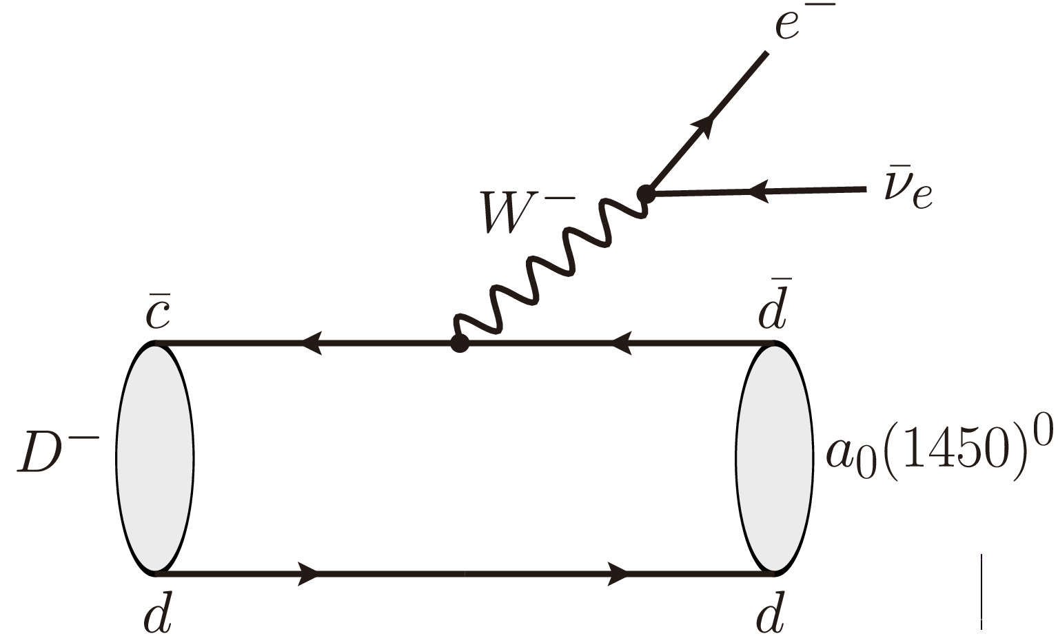
$ a_0(1450) $ can be regarded as a$ q\bar{q} $ state, it exists in three charge configurations with the following quark compositions, respectively:$ a_0(1450)^+={u\bar{d}} $ ,$ a_0(1450)^-={d\bar{u}} $ , and$ a_0(1450)^0= (u\bar{u}-d\bar{d})/\sqrt{2} $ . The differences among them arise from their distinct quark–antiquark flavor compositions. Here we take the semileptonic decay$ D^- \to a_0(1450)^0 \ell^- \bar{\nu}_\ell $ as an example. Its basic mechanism is illustrated by the Feynman diagram shown in Fig. 1, in which the anti-charm quark$ \bar{c} $ transitions to an anti-down quark$ \bar{d} $ via a virtual$ W^- $ boson. Subsequently, the$ W^- $ decays into an$ e^- $ and a$ \bar{\nu}_{e} $ . The spectator d quark does not participate in the weak interaction and finally combines with the produced$ \bar{d} $ to form the light scalar state$ a_0(1450)^0 $ . This decay process can be described by the effective Hamiltonian$ {\cal{H}}_{{\rm{eff}}} = G_F|V_{cd}| \bar{c} \gamma_{\mu}(1-\gamma_{5})d \bar{\ell} \gamma^{\mu}(1-\gamma_{5}) \nu_\ell / \sqrt{2} $ . At the hadronic level, by sandwiching the free-quark amplitude between the initial and final meson states, one can obtain the decay amplitude for the semileptonic$ D \to a_0(1450)\ell \nu_\ell $ . This amplitude consists of a leptonic current and a hadronic current. Since the leptonic current does not participate in strong interactions, it can be calculated straightforwardly. In contrast, the hadronic current involves nonperturbative effects that cannot be computed from first principles. It is usually parameterized in terms of a set of Lorentz-invariant hadronic TFFs,$ i.e., $ 
Figure 1. Feynman diagram representing the tree-level charged-current process
$ D^- \to a_0(1450)^0 \ell^- \bar{\nu}_\ell $ .$ \begin{aligned} \langle a_0(1450)(p)&|\bar{c}\gamma_\mu\gamma_5d|\, D(p+q)\rangle =-i\left[ f_+ (q^2)p_{\mu}+ f_- (q^2)q_{\mu} \right]. \end{aligned} $
(1) Thus, the complex hadronic information has been transformed into a computable quantity. By integrating over phase space, the double-differential decay width, as a function of the squared momentum transfer and the angle between the momenta of the
$ a_0(1450) $ and the lepton$ \ell $ in the lepton-pair center-of-mass frame, can be written as:$ \begin{aligned}[b]& \frac{d^2\Gamma({D \to a_0(1450) \ell \nu_{\ell}})}{dq^2 d\cos\theta_\ell} \\=\;&\frac{G_F^2 |V_{cd}|^2 m_D^3 \lambda^{1/2}}{256 \pi^3 c_{a_0(1450)}^2} \bigg(1-\frac{m_\ell ^2}{q^2} \bigg)^2 \\&\times\bigg\{\lambda |f_+ (q^2)|^2 \bigg[1-\bigg(1-\frac{m_\ell ^2}{q^2} \bigg) {\rm{cos}}^2\theta_\ell \bigg] \\ & +\bigg(1-\frac{m_{a_0(1450)}^2}{m_D^2} \bigg)^2 \frac{m_\ell ^2}{q^2} \\&\times\bigg[ |f_0 (q^2)|^2 +2\lambda^{1/2} {\rm{Re}} [ f_+ (q^2) f_0^*(q^2)]\bigg]\cos\theta_\ell\bigg\}, \end{aligned} $
(2) where
$ G_F = 1.1663787(6)\times 10^{-5} {\rm{GeV}}^{-2} $ is the Fermi coupling constant,$ m_\ell $ is the lepton mass, and$ \lambda\equiv\lambda(1,m_{a_0(1450)}^2/m_D^2,q^2/m_D^2) $ with$ \lambda(a,b,c)\equiv a^2+b^2+c^2- 2(ab+ac+bc) $ . Meanwhile, the scalar TFF is related to the traditional vector TFFs, i.e.$ f_0 (q^2)=f_+ (q^2)+{q^2}/ (m_D^2-m_{a_0(1450)}^2) f_- (q^2) $ . Specifically, the isospin factor$ c_{a_0(1450)} = \sqrt{2} $ corresponds to$ D^- \to a_0(1450)^0 \ell^- \bar{\nu}_\ell $ , while$ c_{a_0(1450)} = 1 $ corresponds to$ D^0 \to a_0(1450)^- \ell^+ \bar{\nu}_\ell $ , reflecting the different electric charges. In general, the differential decay width provides an important bridge between theory and experiment and is also an effective means of testing the SM. On the other hand, one can also focus on the angular distribution of the differential decay width, along with three angular observables that are highly sensitive to new physics,$ i.e., $ the forward-backward asymmetry$ {\cal{A}}_{\rm{FB}}(q^2) $ , the lepton polarization asymmetry$ {\cal{A}}_{\lambda_\ell} $ , and the$ q^2 $ -differential flat term$ {\cal{F}}_{\rm{H}}(q^2) $ . For brevity, their specific expressions are not presented here and can be found in Ref. [55].In order to derive the
$ D \to a_0(1450) $ TFFs based on the QCD LCSR, one can start from the two-point correlation function from the vacuum to the final-state light$ a_0(1450) $ state,$ \Pi_{\mu}(p,q) = i\int d^4x e^{iq\cdot x} \langle a_0(1450)(p)|T\{J_n(x), j_n^{\dagger}(0)\}|0 \rangle, $
(3) where the current operators
$ J_n(x)=\bar{q}_2(x) \gamma_{\mu} \gamma_{5} c(x) $ describe the weak transition$ c\to q_2 $ , and$ j_{n}^{\dagger}(0)=\bar{c} i\gamma_{5} q_1(0) $ represents the D-meson decay channel. Here,$ q_1 $ and$ q_2 $ denote light quarks. This correlation function can be analyzed in different kinematic regions, allowing for a consistent matching between its phenomenological representation and its theoretical expression. The procedure is as follows: First, in the time-like$ q^2 $ region, we insert a complete set of intermediate states with D-meson quantum numbers to obtain the hadronic representation.$ \begin{aligned}[b] \Pi_{\mu}^{{\rm{had}}}(p,q) =\;& \frac{\langle a_0(1450)|\bar{q}_2 \gamma_\mu \gamma_5 c|D\rangle\langle D|\bar{c}i\gamma_5 q|0\rangle}{m_D^2 - (p+q)^2} \\&+ \sum_{\rm{H}} \frac{\langle a_0(1450)|\bar{q}_2 \gamma_\mu \gamma_5 c|D^{\rm{H}}\rangle\langle D^{\rm{H}}|\bar{c}i\gamma_5 q_1|0\rangle}{m_{D^{{\rm{H}}}}^2 - (p+q)^2}, \end{aligned} $
(4) where the vacuum-to-meson matrix element is defined as
$ \langle D|\bar{c}i\gamma_5 q_1 |0\rangle =m^2_D f_D/m_c $ . With this definition, we can further derive$ \begin{aligned}[b] \Pi_{\mu}(p,q) =\;& \frac{m_{D}^2 f_{D}}{m_c \left[m_{D}^2 - (p+q)^2\right]} \left[f_+(q^2)p_{\mu} + f_-(q^2)q_{\mu}\right] \\&+ \int_{s_0 }^{\infty} ds \frac{\rho_+^{\rm{H}}(s)p_{\mu} + \rho_-^{\rm{H}}(s)q_{\mu}}{s - (p+q)^2}. \end{aligned} $
(5) Here, the ground-state contribution is isolated. The contributions from higher resonances and continuum states are modeled by the spectral density function
$ \rho_{+,-}^{\rm{H}}(s) $ . Owing to the complexity of multi-hadron continuum states at high energies, it is difficult to obtain an explicit analytic expression for this function. To address this, we invoke quark-hadron duality to relate it to the corresponding QCD representation.$ \rho^{\rm{H}}_{+,-}(s) = \rho^{\rm{QCD}}_{+,-}(s)\theta(s - s_0). $
(6) Additionally, the correlation function can be computed in the deep Euclidean region
$ q^2=-Q^2\ll 0 $ using the operator product expansion (OPE) near the light-cone ($ x^2 \approx 0 $ ). The QCD expression is then obtained by contracting the heavy c quark field to its full quark propagator.$ \begin{aligned} \langle 0|c_{\alpha}^{j}(x)\bar{c}_{\beta}^{j}(0)|0\rangle &= i \int \frac{d^4k}{(2\pi)^4} e^{-ik\cdot x} \left[ \delta^{ij} \frac{\not{k} + m_c}{k^2 - m_c^2} + \cdots \right]_{\alpha\beta}. \end{aligned} $
(7) The first term corresponds to the free quark propagator, which provides the leading contribution. The second term arises from the one-gluon exchange contribution, which generally does not play a significant role in the sum rules for TFFs and can be safely neglected. Currently, the twist-4 LCDAs of scalar
$ q\bar{q} $ states such as$ a_0(1450) $ are still not well established. Therefore, we retain only the twist-2 and twist-3 LCDAs in this paper, which have been widely studied using other approaches. After substituting the free quark propagator into the correlation function, we obtain the OPE results. By applying a Borel transformation and employing dispersion relations to match the QCD representation with the hadronic representation, the final analytical expressions for the TFFs within the LCSR framework can be written as$ \begin{aligned}[b] f_+^{({\rm{S}}1, {\rm{S}}2)} (q^2) =\;& \frac{m_c \; \bar{f}_{a_0(1450)}}{m_D^2 f_D} \; \int_{u_0}^1 \; du \; e^{(m_{D}^2 -s(u))/M^2} \; \bigg\{-\frac{m_c}{u} \; \phi^{({\rm{S}}1, {\rm{S}}2)}_{2;a_0(1450)}(u,\mu) \,+\, m_{a_0(1450)} \times \phi_{3;a_0(1450)}^p(u,\mu) +\frac{m_{a_0(1450)}}{6} \\ &\times\bigg[ \frac{2}{u} \phi_{3;a_0(1450)}^\sigma(u,\mu)-\bigg(\frac{m_c^2-u^2 m_{a_0(1450)}^2 +q^2}{m_c^2 +u^2 m_{a_0(1450)}^2 -q^2} \times \frac{d\phi_{3;a_0(1450)}^\sigma(u,\mu)}{du} - \frac{4u m_c^2 m_{a_0(1450)}^2}{(m_c^2 +u^2 m_{a_0(1450)}^2 -q^2)^2} \phi_{3;a_0(1450)}^\sigma(u,\mu) \bigg) \bigg] \bigg\}, \end{aligned} $
(8) $ \begin{aligned} &f_- (q^2) = \frac{ \bar{f}_{a_0(1450)}}{m_D^2 f_D} \int_{u_0}^1 du e^{(m_{D}^2 - s(u))/M^2} \bigg[ \frac{m_c}{u} {\phi_{3;a_0(1450)}^p (u,\mu)} +\frac{m_c}{6u} \frac{d\phi_{3;a_0(1450)}^\sigma(u,\mu)}{du} \bigg], \end{aligned} $
(9) where the lower limit of integration is
$ u_0 = \{ [(s- q^2- m_{a_0(1450)}^2)^2 +4m_{a_0(1450)}^2(m_{c}^2-q^2)]^{1/2}-(s-q^2-m_{a_0(1450)}^2) \}/(2m_{a_0(1450)}^2), $ $ s(u) = (m_c^2 +u\bar{u}m_{a_0(1450)}^2 -\bar{u}q^2)/u $ with$ \bar{u}=(1-u) $ . Here,$ m_D $ and$ f_D $ denote the mass and decay constant of the D meson, respectively;$ m_c $ is the mass of the c quark;$ s_0 $ represents the continuum threshold parameter; and$ M^2 $ is the Borel parameter.As the main source of nonperturbative uncertainty in LCSR expressions, the twist-2 LCDA of
$ a_0(1450) $ is a universal nonperturbative quantity; therefore, it is appropriate to study it using nonperturbative QCD methods. In general, the exploration of$ \phi_{2;a_0}(x,\mu) $ can be carried out by combining nonperturbative QCD with phenomenological models. Thus, with the π-meson wave function as a reference and the Brodsky-Huang-Lepage (BHL) hypothesis as a starting point, we establish a specific correspondence between the equal-time wave function in the rest frame and the light-cone wave function [56, 57], which can be expressed as follows:$ \Psi_{2; a_0(1450)}(x,{\bf{k}}_{\perp}) = \sum\limits_{\lambda_1\lambda_2} \chi_{a_0(1450)}^{\lambda_1\lambda_2}(x,{\bf{k}}_{\perp})\psi_{a_0(1450)}^R(x,{\bf{k}}_{\perp}). $
(10) For the spin wave function
$ \chi_{a_0(1450)}^{\lambda_1\lambda_2}(x,{\bf{k}}_{\perp}) $ , the light-meson wave function is usually transformed to the light-cone form to obtain the complete spin wave function within the instant-form SU(6) quark model [54, 58, 59]. Starting from the instant form, we consider the scalar state$ a_0(1450) $ with spin$ S=1 $ , orbital angular momentum$ L=1 $ , and total angular momentum$ J=0 $ . In the rest frame$ ({\boldsymbol{q}}_1 +{\boldsymbol{q}}_2 =0) $ , the spin wave function in the instant form (T) can be obtained.$ \chi_{a_0(1450)}^T=\frac{1}{\sqrt{2}}(\chi_1^\uparrow\chi_2^\downarrow- \chi_2^\uparrow\chi_1^\downarrow), $
(11) where
$ \chi_{1/2}^{\uparrow/\downarrow} $ denotes the two-component Pauli spinor, and the four-momenta of the two quarks are, respectively,$ q^{\mu}_1 =(q^0,{\boldsymbol{q}}) $ and$ q^{\mu}_2 =(q^0,-{\boldsymbol{q}}) $ , with$ q^0=\sqrt{m^2 +{\boldsymbol{q}}^2} $ . The spin wave function is a function of the constituent quark mass and the transverse momentum. After integrating over the transverse momentum, the spin wave function depends only on the factorization scale μ. In contrast, the spatial wave function is governed by the three free parameters A, β, and α. At a fixed scale μ, the twist-2 LCDA of$ a_0(1450) $ is primarily determined by the spatial wave function, while the contribution from the spin wave function is negligible. Therefore, we take guidance from the spin-wave-function structure of the pseudoscalar π meson and adopt an approximate form for the twist-2 spin wave function of$ a_0(1450) $ . This approximation has also been adopted in other scalar-state studies [60−62]. The instant-form$ \vert J, s \rangle_T $ and the light-cone form$ \vert J, \lambda \rangle_F $ are related by a Wigner rotation. For hadronic states with total angular momentum$ J=0 $ , this rotation reduces to the identity, and can be written as$ |J,\lambda \rangle_F=\sum_s U_{s \lambda}^J |J,s \rangle_T $ . For a quark with spin-1/2, the corresponding Melosh transformation is given as follows:$\begin{aligned}[b] & \chi^\uparrow(T)=\omega[(q^++m)\chi^\uparrow(F)-q_R\chi^\downarrow(F)], \\& \chi^\downarrow(T)=\omega[(q^++m)\chi^\downarrow(F)+q_L\chi^\uparrow(F)], \end{aligned}$
(12) where
$ \omega=[2q^+(q^0+m)]^{-1/2}, q_{R/L}=q_1\pm iq_2, q^+=q^0+q^3 $ . Then, the spin wave function of the$ a_0(1450) $ state can be obtained,$ \chi_{a_0(1450)}(x,{\bf{k}}_\perp)=\sum\limits_{\lambda_1,\lambda_2}C_0^F(x,{\bf{k}}_\perp, \lambda_1,\lambda_2)\chi_{1}^{\lambda_1}(F)\chi_{2}^{\lambda_2}(F). $
(13) Expressed in terms of the instant-form momentum
$ q^\mu=(q^0,{\boldsymbol{q}}) $ , the component coefficient$ C_{0}^F(x,{\bf{k}}_\perp,\lambda_1,\lambda_2) $ can be computed; its explicit form is:$ \begin{aligned}[b] C_0^F(x,{\bf{k}}_\perp,\uparrow,\downarrow)&= + \frac{m}{\sqrt{2(m^2+{\bf{k}}_{\perp}^2)}}, \\ C_0^F(x,{\bf{k}}_\perp,\downarrow,\uparrow)&=-\frac{m}{\sqrt{2\big(m^2+{\bf{k}}_{\perp}^2)}}, \\ C_0^F(x,{\bf{k}}_\perp,\uparrow,\uparrow)&=- \frac{(k_1-ik_2)}{\sqrt{2(m ^2+{\bf{k}}_\perp^2)}}, \\ C_0^F(x,{\bf{k}}_\perp,\downarrow,\downarrow)&=-\frac{(k_1+ik_2)}{\sqrt{2(m^2+{\bf{k}}_\perp^2)}}, \end{aligned} $
(14) These coefficients satisfy the following normalization relation:
$ \sum_{\lambda_{1},\lambda_{2}}C_{0}^{F}(x,{\bf{k}}_{\perp},\lambda_{1},\lambda_{2})^* C_{0}^{F}(x,{\bf{k}}_{\perp},\lambda_{1},\lambda_{2})=1 $ . In addition to the ordinary helicity component$ (\lambda_1 +\lambda_2=0) $ , higher helicity components$ (\lambda_1 +\lambda_2 = \pm1) $ also exist, whereas the instant-form wave function contains only the ordinary helicity component. The spin wave function can then be defined as:$ \chi_{a_0(1450)}^{\lambda_1\lambda_2}(x,{\bf{k}}_{\perp})= \frac{\hat{m}_q^2}{\sqrt{{\bf{k}}_\perp^2 + \hat{m}_q^2}}. $
(15) Moreover, the BHL description establishes an equivalence between the spatial wave function
$ \Psi_{2;a_0(1450)}^R(x,{\bf{k}}_{\perp}) $ and the equal-time wave function, thereby avoiding the complex task of solving an infinite set of coupled integral equations to determine the specific form of the wave function. This leads us to the following result:$ \psi_{2;a_0(1450)}^R(x,{\bf{k}}_{\perp}) = A \varphi_{a_0(1450)}(x) \exp \Big[ - \frac{{\bf{k}}_\perp^2 + \hat{m}_q^2}{8 \beta^2 {x}{\bar{x}}} \Big], $
(16) where
$ {\bf{k}}_\perp $ denotes the transverse momentum, and A and$ \hat{m}_q $ denote the normalization constant and the light-quark mass, respectively [63, 64]. According to Ref. [65], the harmonic-oscillator exponential factor$ \exp [-({\bf{k}}_\perp^2+m_q^2)/ (8\beta^2x\bar{x})] $ primarily controls the broadening in the transverse momentum$ {\bf{k}}_\perp $ . On the other hand, accounting for quark spin introduces additional corrections to the longitudinal distribution of the distribution amplitude. To this end, we can control the longitudinal distribution by introducing the function$ \varphi_{a_0(1450)}(x) $ , which allows adjustment of the shape in x (including endpoint behavior and width) of the twist-2 LCDA of$ a_0(1450) $ . Usually, a form similar to the traditional Gegenbauer polynomial expansion is adopted. Building on this, we consider the first scheme:$ \begin{aligned} &\varphi^{({\rm{S}}1)}_{a_0(1450)}(x)=C_1^{3/2}(x-\bar x), \end{aligned} $
(17) Since the twist-2 distribution amplitude of the scalar state
$ a_0(1450) $ is antisymmetric under the exchange$ x\leftrightarrow(1-x) $ , the zeroth Gegenbauer moment vanishes. To more comprehensively assess the model's applicability, we also consider the second scheme:$ \varphi^{({\rm{S}}2)}_{a_0(1450)}(x)=(x\bar{x})^{\alpha}C_1^{3/2}(x-\bar x). $
(18) This structure is optimized by introducing a factor
$ (x \bar{x})^{\alpha} $ . This factor ensures that the expression approaches the theoretical limit$ (x \bar{x})^{\alpha}=6x\bar{x} $ as$ \mu \to \infty $ [66].After integrating over the transverse momentum
$ {\bf{k}}_{\perp} $ , the final twist-2 LCDA of the$ a_0(1450) $ is obtained.$ \begin{aligned}[b] \phi^{({\rm{S}}1, {\rm{S}}2)}_{2;a_0(1450)}(x,\mu) =\;& \frac{A \hat{m}_q \beta}{4 \sqrt{2} \pi^{3/2}} \sqrt{x \bar{x}} \varphi^{({\rm{S}}1, {\rm{S}}2)}_{a_0(1450)}(x) \\&\times\left\{{\rm{Erf}}\left[\sqrt{\frac{\hat{m}_q^2 + \mu^2}{8\beta^2 x\bar{x}}} \right]-{\rm{Erf}}\left[\sqrt{\frac{\hat{m}_q^2}{8\beta^2 x\bar{x}}}\right]\right\}, \end{aligned} $
(19) where
$ {\rm{Erf}}(x) = 2{\int_{0}^{x}e^{-t^2}dx}/{\sqrt{\pi}} $ denotes the error function, and we set$ \hat{m}_q = 250\; {\rm{MeV}} $ . The model parameters in the two amplitude schemes above can be determined using the following criteria:● The average value of the squared transverse momentum,
$ \langle {\bf{k}}_{\perp}^2\rangle $ [67], is given by:$ \langle{\bf{k}}_\perp^2\rangle = \frac{\int dxd^2{\bf{k}}_\perp|{\bf{k}}_\perp|^2|\Psi_{2; a_0(1450)}^{({\rm{S}}1, {\rm{S}}2)}(x,{\bf{k}}_{\perp})|^2}{\int dxd^2{\bf{k}}_\perp|\Psi_{2; a_0(1450)}^{({\rm{S}}1, {\rm{S}}2)}(x,{\bf{k}}_{\perp})|^2}, $
(20) which is consistent with the choice in Ref. [57] for light scalar states or light mesons.
● The Gegenbauer moments
$ a_n^{({\rm{S}}1, {\rm{S}}2)}(\mu) $ can be derived as follows [68]:$ a_n^{({\rm{S}}1, {\rm{S}}2)} (\mu)=\frac{\int_0^1dx\phi_{2;a_0(1450)}^{({\rm{S}}1, {\rm{S}}2)} (x,\mu)C_n^{3/2}(\xi)}{\int_0^1 dx 6x\bar{x}[C_n^{3/2}(\xi)]^2}, $
(21) where
$ \xi=(2x-1) $ . In general, the properties of the twist-2 LCDA are primarily determined by its first few terms.For the first scheme, we adopt the first-order Gegenbauer moment and the average squared transverse momentum
$ \langle {\bf{k}}_{\perp}^2\rangle $ to determine the model parameters$ A^{({\rm{S}}1)} $ and$ \beta^{({\rm{S}}1)} $ . For the model parameters$ A^{({\rm{S}}2)} $ ,$ \beta^{({\rm{S}}2)} $ , and$ \alpha^{({\rm{S}}2)} $ in the second scheme, we adopt$ \langle {\bf{k}}_{\perp}^2\rangle $ and the first and third-order Gegenbauer moments. For the$ a_0(1450) $ twist-2 LCDA$ \phi_{2;a_0(1450)}^{({\rm{S}}1, {\rm{S}}2)}(x,\mu) $ , the nth-order moment$ \langle\xi^{n}\rangle|_\mu^{({\rm{S}}1, {\rm{S}}2)} $ – an important quantity for the nonperturbative momentum distribution – is defined as$ \langle\xi^{n}\rangle|_\mu^{({\rm{S}}1, {\rm{S}}2)}=\int_0^1 dx(2x-1)^{n}\phi_{2;a_0(1450)}^{({\rm{S}}1, {\rm{S}}2)}(x,\mu). $
(22) To facilitate comparison with the LCHO model, we also adopt the truncated distribution amplitude of the
$ a_0(1450) $ state and substitute it into our TFFs to compute the resulting physical observables [1].$ \phi_{2;a_0(1450)}^{\rm{TF}}(x,\mu)=6x\bar{x}\left[a_0(\mu)+\sum\limits_{n=1}^{{\cal{N}}=3}a_n(\mu) C_n^{3/2}(\xi)\right]. $
(23) Finally, the twist-3 LCDAs of the
$ a_0(1450) $ can be expanded in a series of Gegenbauer polynomials and truncated to retain only the first few terms; the explicit form is as follows [69]:$ \begin{aligned}[b] \phi_{3;a_0(1450)}^{p}(x,\mu) &= 1+\sum\limits_{n=1}^{{\cal{N}}=2} a_{n}^{p}(\mu) C_{n}^{1/2}(\xi), \\ \phi_{3;a_0(1450)}^{\sigma}(x,\mu) &= 6x\bar{x} \bigg[1+\sum\limits_{n=1}^{{\cal{N}}=2} a_{n}^{\sigma}(\mu) C_{n}^{3/2}(\xi) \bigg]. \end{aligned} $
(24) Using the aforementioned twist-3 distribution amplitudes as input parameters, we obtain the complete set of TFFs.
-
Assuming that the light scalar state
$ a_0(1450) $ can be regarded as a$ q\bar{q} $ state, it exists in three charge configurations with the following quark compositions, respectively:$ a_0(1450)^+={u\bar{d}} $ ,$ a_0(1450)^-={d\bar{u}} $ , and$ a_0(1450)^0= (u\bar{u}-d\bar{d})/\sqrt{2} $ . The differences among them arise from their distinct quark–antiquark flavor compositions. Here we take the semileptonic decay$ D^- \to a_0(1450)^0 \ell^- \bar{\nu}_\ell $ as an example. Its basic mechanism is illustrated by the Feynman diagram shown in Fig. 1, in which the anti-charm quark$ \bar{c} $ transitions to an anti-down quark$ \bar{d} $ via a virtual$ W^- $ boson. Subsequently, the$ W^- $ decays into an$ e^- $ and a$ \bar{\nu}_{e} $ . The spectator d quark does not participate in the weak interaction and finally combines with the produced$ \bar{d} $ to form the light scalar state$ a_0(1450)^0 $ . This decay process can be described by the effective Hamiltonian$ {\cal{H}}_{{\rm{eff}}} = G_{\rm F}|V_{cd}| \bar{c} \gamma_{\mu}(1-\gamma_{5})d \bar{\ell} \gamma^{\mu}(1-\gamma_{5}) \nu_\ell / \sqrt{2} $ . At the hadronic level, by sandwiching the free-quark amplitude between the initial and final meson states, one can obtain the decay amplitude for the semileptonic$ D \to a_0(1450)\ell \nu_\ell $ . This amplitude consists of a leptonic current and a hadronic current. Since the leptonic current does not participate in strong interactions, it can be calculated straightforwardly. In contrast, the hadronic current involves nonperturbative effects that cannot be computed from first principles. It is usually parameterized in terms of a set of Lorentz-invariant hadronic TFFs,$ i.e., $
Figure 1. Feynman diagram representing the tree-level charged-current process
$ D^- \to a_0(1450)^0 \ell^- \bar{\nu}_\ell $ .$ \begin{aligned} \langle a_0(1450)(p)&|\bar{c}\gamma_\mu\gamma_5d|\, D(p+q)\rangle =- {\rm i} \left[ f_+ (q^2)p_{\mu}+ f_- (q^2)q_{\mu} \right]. \end{aligned} $
(1) Thus, the complex hadronic information has been transformed into a computable quantity. By integrating over phase space, the double-differential decay width, as a function of the squared momentum transfer and the angle between the momenta of the
$ a_0(1450) $ and the lepton$ \ell $ in the lepton-pair center-of-mass frame, can be written as:$ \begin{aligned}[b]& \frac{{\rm d}^2\Gamma({D \to a_0(1450) \ell \nu_{\ell}})}{{\rm d}q^2 {\rm d}\cos\theta_\ell} \\=\;&\frac{G_{\rm F}^2 |V_{cd}|^2 m_D^3 \lambda^{1/2}}{256 \pi^3 c_{a_0(1450)}^2} \bigg(1-\frac{m_\ell ^2}{q^2} \bigg)^2 \\&\times\bigg\{\lambda |f_+ (q^2)|^2 \bigg[1-\bigg(1-\frac{m_\ell ^2}{q^2} \bigg) {\rm{cos}}^2\theta_\ell \bigg] \\ & +\bigg(1-\frac{m_{a_0(1450)}^2}{m_D^2} \bigg)^2 \frac{m_\ell ^2}{q^2} \\&\times\bigg[ |f_0 (q^2)|^2 +2\lambda^{1/2} {\rm{Re}} [ f_+ (q^2) f_0^*(q^2)]\bigg]\cos\theta_\ell\bigg\}, \end{aligned} $
(2) where
$ G_{\rm F} = 1.1663787(6)\times 10^{-5} {\rm{GeV}}^{-2} $ is the Fermi coupling constant,$ m_\ell $ is the lepton mass, and$ \lambda\equiv\lambda(1, m_{a_0(1450)}^2/m_D^2, \; q^2/m_D^2) $ with$ \lambda(a,b,c)\equiv a^2+b^2+c^2- 2(ab+ ac+ bc) $ . Meanwhile, the scalar TFF is related to the traditional vector TFFs, i.e.$ f_0 (q^2)=f_+ (q^2)+{q^2}/ (m_D^2- m_{a_0(1450)}^2) \times f_- (q^2) $ . Specifically, the isospin factor$ c_{a_0(1450)} = \sqrt{2} $ corresponds to$ D^- \to a_0(1450)^0 \ell^- \bar{\nu}_\ell $ , while$ c_{a_0(1450)} = 1 $ corresponds to$ D^0 \to a_0(1450)^- \ell^+ \bar{\nu}_\ell $ , reflecting the different electric charges. In general, the differential decay width provides an important bridge between theory and experiment and is also an effective means of testing the SM. On the other hand, one can also focus on the angular distribution of the differential decay width, along with three angular observables that are highly sensitive to new physics,$ i.e., $ the forward-backward asymmetry$ {\cal{A}}_{\rm{FB}}(q^2) $ , the lepton polarization asymmetry$ {\cal{A}}_{\lambda_\ell} $ , and the$ q^2 $ -differential flat term$ {\cal{F}}_{\rm{H}}(q^2) $ . For brevity, their specific expressions are not presented here and can be found in Ref. [55].In order to derive the
$ D \to a_0(1450) $ TFFs based on the QCD LCSR, one can start from the two-point correlation function from the vacuum to the final-state light$ a_0(1450) $ state,$ \Pi_{\mu}(p,q) = {\rm i}\int {\rm d}^4x {\rm e}^{{\rm i}q\cdot x} \langle a_0(1450)(p)|T\{J_n(x), j_n^{\dagger}(0)\}|0 \rangle, $
(3) where the current operators
$ J_n(x)=\bar{q}_2(x) \gamma_{\mu} \gamma_{5} c(x) $ describe the weak transition$ c\to q_2 $ , and$ j_{n}^{\dagger}(0)=\bar{c} {\rm i}\gamma_{5} q_1(0) $ represents the D-meson decay channel. Here,$ q_1 $ and$ q_2 $ denote light quarks. This correlation function can be analyzed in different kinematic regions, allowing for a consistent matching between its phenomenological representation and its theoretical expression. The procedure is as follows: First, in the time-like$ q^2 $ region, we insert a complete set of intermediate states with D-meson quantum numbers to obtain the hadronic representation.$ \begin{aligned}[b] \Pi_{\mu}^{{\rm{had}}}(p,q) =\;& \frac{\langle a_0(1450)|\bar{q}_2 \gamma_\mu \gamma_5 c|D\rangle\langle D|\bar{c}{\rm i}\gamma_5 q|0\rangle}{m_D^2 - (p+q)^2} \\&+ \sum_{\rm{H}} \frac{\langle a_0(1450)|\bar{q}_2 \gamma_\mu \gamma_5 c|D^{\rm{H}}\rangle\langle D^{\rm{H}}|\bar{c}{\rm i}\gamma_5 q_1|0\rangle}{m_{D^{{\rm{H}}}}^2 - (p+q)^2}, \end{aligned} $
(4) where the vacuum-to-meson matrix element is defined as
$ \langle D|\bar{c}{\rm i}\gamma_5 q_1 |0\rangle =m^2_D f_D/m_c $ . With this definition, we can further derive$ \begin{aligned}[b] \Pi_{\mu}(p,q) =\;& \frac{m_{D}^2 f_{D}}{m_c \left[m_{D}^2 - (p+q)^2\right]} \left[f_+(q^2)p_{\mu} + f_-(q^2)q_{\mu}\right] \\&+ \int_{s_0 }^{\infty} {\rm d}s \frac{\rho_+^{\rm{H}}(s)p_{\mu} + \rho_-^{\rm{H}}(s)q_{\mu}}{s - (p+q)^2}. \end{aligned} $
(5) Here, the ground-state contribution is isolated. The contributions from higher resonances and continuum states are modeled by the spectral density function
$ \rho_{+,-}^{\rm{H}}(s) $ . Owing to the complexity of multi-hadron continuum states at high energies, it is difficult to obtain an explicit analytic expression for this function. To address this, we invoke quark-hadron duality to relate it to the corresponding QCD representation.$ \rho^{\rm{H}}_{+,-}(s) = \rho^{\rm{QCD}}_{+,-}(s)\theta(s - s_0). $
(6) Additionally, the correlation function can be computed in the deep Euclidean region
$ q^2=-Q^2\ll 0 $ using the operator product expansion (OPE) near the light-cone ($ x^2 \approx 0 $ ). The QCD expression is then obtained by contracting the heavy c quark field to its full quark propagator.$ \begin{aligned} \langle 0|c_{\alpha}^{j}(x)\bar{c}_{\beta}^{j}(0)|0\rangle &= {\rm i} \int \frac{{\rm d}^4k}{(2\pi)^4} {\rm e}^{-{\rm i}k\cdot x} \left[ \delta^{ij} \frac{\not{k} + m_c}{k^2 - m_c^2} + \cdots \right]_{\alpha\beta}. \end{aligned} $
(7) The first term corresponds to the free quark propagator, which provides the leading contribution. The second term arises from the one-gluon exchange contribution, which generally does not play a significant role in the sum rules for TFFs and can be safely neglected. Currently, the twist-4 LCDAs of scalar
$ q\bar{q} $ states such as$ a_0(1450) $ are still not well established. Therefore, we retain only the twist-2 and twist-3 LCDAs in this paper, which have been widely studied using other approaches. After substituting the free quark propagator into the correlation function, we obtain the OPE results. By applying a Borel transformation and employing dispersion relations to match the QCD representation with the hadronic representation, the final analytical expressions for the TFFs within the LCSR framework can be written as$ \begin{aligned}[b] f_+^{({\rm{S}}1, {\rm{S}}2)} (q^2) =\;& \frac{m_c \, \bar{f}_{a_0(1450)}}{m_D^2 f_D} \int_{u_0}^1 \, {\rm d}u \, {\rm e}^{(m_{D}^2 -s(u))/M^2} \bigg\{-\frac{m_c}{u} \, \phi^{({\rm{S}}1, {\rm{S}}2)}_{2;a_0(1450)}(u,\mu) \,+\, m_{a_0(1450)} \phi_{3;a_0(1450)}^p(u,\mu) +\frac{m_{a_0(1450)}}{6} \\ & \times \bigg[ \frac{2}{u} \phi_{3;a_0(1450)}^\sigma(u,\mu)-\bigg(\frac{m_c^2-u^2 m_{a_0(1450)}^2 +q^2}{m_c^2 +u^2 m_{a_0(1450)}^2 -q^2} \frac{{\rm d} \phi_{3;a_0(1450)}^\sigma(u,\mu)}{{\rm d}u} - \frac{4u m_c^2 m_{a_0(1450)}^2}{(m_c^2 +u^2 m_{a_0(1450)}^2 -q^2)^2} \phi_{3;a_0(1450)}^\sigma(u,\mu) \bigg) \bigg] \bigg\}, \end{aligned} $
(8) $ \begin{aligned} &f_- (q^2) = \frac{ \bar{f}_{a_0(1450)}}{m_D^2 f_D} \int_{u_0}^1 {\rm d} u {\rm e}^{(m_{D}^2 - s(u))/M^2} \bigg[ \frac{m_c}{u} {\phi_{3;a_0(1450)}^p (u,\mu)} +\frac{m_c}{6u} \frac{{\rm d}\phi_{3;a_0(1450)}^\sigma(u,\mu)}{{\rm d}u} \bigg], \end{aligned} $
(9) where the lower limit of integration is
$ u_0 = \{ [(s- q^2- m_{a_0(1450)}^2)^2 +4m_{a_0(1450)}^2(m_{c}^2-q^2)]^{1/2}-(s-q^2-m_{a_0(1450)}^2) \}/(2m_{a_0(1450)}^2), $ $ s(u) = (m_c^2 +u\bar{u}m_{a_0(1450)}^2 -\bar{u}q^2)/u $ with$ \bar{u}=(1-u) $ . Here,$ m_D $ and$ f_D $ denote the mass and decay constant of the D meson, respectively;$ m_c $ is the mass of the c quark;$ s_0 $ represents the continuum threshold parameter; and$ M^2 $ is the Borel parameter.As the main source of nonperturbative uncertainty in LCSR expressions, the twist-2 LCDA of
$ a_0(1450) $ is a universal nonperturbative quantity; therefore, it is appropriate to study it using nonperturbative QCD methods. In general, the exploration of$ \phi_{2;a_0}(x,\mu) $ can be carried out by combining nonperturbative QCD with phenomenological models. Thus, with the π-meson wave function as a reference and the Brodsky-Huang-Lepage (BHL) hypothesis as a starting point, we establish a specific correspondence between the equal-time wave function in the rest frame and the light-cone wave function [56, 57], which can be expressed as follows:$ \Psi_{2; a_0(1450)}(x,{\bf{k}}_{\perp}) = \sum\limits_{\lambda_1\lambda_2} \chi_{a_0(1450)}^{\lambda_1\lambda_2}(x,{\bf{k}}_{\perp})\psi_{a_0(1450)}^R(x,{\bf{k}}_{\perp}). $
(10) For the spin wave function
$ \chi_{a_0(1450)}^{\lambda_1\lambda_2}(x,{\bf{k}}_{\perp}) $ , the light-meson wave function is usually transformed to the light-cone form to obtain the complete spin wave function within the instant-form SU(6) quark model [54, 58, 59]. Starting from the instant form, we consider the scalar state$ a_0(1450) $ with spin$ S=1 $ , orbital angular momentum$ L=1 $ , and total angular momentum$ J=0 $ . In the rest frame$ ({\boldsymbol{q}}_1 +{\boldsymbol{q}}_2 =0) $ , the spin wave function in the instant form (T) can be obtained.$ \chi_{a_0(1450)}^T=\frac{1}{\sqrt{2}}(\chi_1^\uparrow\chi_2^\downarrow- \chi_2^\uparrow\chi_1^\downarrow), $
(11) where
$ \chi_{1/2}^{\uparrow/\downarrow} $ denotes the two-component Pauli spinor, and the four-momenta of the two quarks are, respectively,$ q^{\mu}_1 =(q^0,{\boldsymbol{q}}) $ and$ q^{\mu}_2 =(q^0,-{\boldsymbol{q}}) $ , with$ q^0=\sqrt{m^2 +{\boldsymbol{q}}^2} $ . The spin wave function is a function of the constituent quark mass and the transverse momentum. After integrating over the transverse momentum, the spin wave function depends only on the factorization scale μ. In contrast, the spatial wave function is governed by the three free parameters A, β, and α. At a fixed scale μ, the twist-2 LCDA of$ a_0(1450) $ is primarily determined by the spatial wave function, while the contribution from the spin wave function is negligible. Therefore, we take guidance from the spin-wave-function structure of the pseudoscalar π meson and adopt an approximate form for the twist-2 spin wave function of$ a_0(1450) $ . This approximation has also been adopted in other scalar-state studies [60−62]. The instant-form$ \vert J, s \rangle_T $ and the light-cone form$ \vert J, \lambda \rangle_{\rm F} $ are related by a Wigner rotation. For hadronic states with total angular momentum$ J=0 $ , this rotation reduces to the identity, and can be written as$ |J,\lambda \rangle_{\rm F}=\sum_s U_{s \lambda}^J |J,s \rangle_T $ . For a quark with spin-1/2, the corresponding Melosh transformation is given as follows:$\begin{aligned}[b] & \chi^\uparrow(T)=\omega[(q^++m)\chi^\uparrow(F)-q_R\chi^\downarrow(F)], \\& \chi^\downarrow(T)=\omega[(q^++m)\chi^\downarrow(F)+q_L\chi^\uparrow(F)], \end{aligned}$
(12) where
$ \omega=[2q^+(q^0+m)]^{-1/2}, \;\; q_{R/L}=q_1\pm {\rm i}q_2, \;\; q^+=q^0+q^3 $ . Then, the spin wave function of the$ a_0(1450) $ state can be obtained,$ \chi_{a_0(1450)}(x,{\bf{k}}_\perp)=\sum\limits_{\lambda_1,\lambda_2}C_0^F(x,{\bf{k}}_\perp, \lambda_1,\lambda_2)\chi_{1}^{\lambda_1}(F)\chi_{2}^{\lambda_2}(F). $
(13) Expressed in terms of the instant-form momentum
$ q^\mu=(q^0,{\boldsymbol{q}}) $ , the component coefficient$ C_{0}^F(x,{\bf{k}}_\perp,\lambda_1,\lambda_2) $ can be computed; its explicit form is:$ \begin{aligned}[b] C_0^F(x,{\bf{k}}_\perp,\uparrow,\downarrow)&= + \frac{m}{\sqrt{2(m^2+{\bf{k}}_{\perp}^2)}}, \\ C_0^F(x,{\bf{k}}_\perp,\downarrow,\uparrow)&=-\frac{m}{\sqrt{2\big(m^2+{\bf{k}}_{\perp}^2)}}, \\ C_0^F(x,{\bf{k}}_\perp,\uparrow,\uparrow)&=- \frac{(k_1-{\rm i}k_2)}{\sqrt{2(m ^2+{\bf{k}}_\perp^2)}}, \\ C_0^F(x,{\bf{k}}_\perp,\downarrow,\downarrow)&=-\frac{(k_1+{\rm i}k_2)}{\sqrt{2(m^2+{\bf{k}}_\perp^2)}}, \end{aligned} $
(14) These coefficients satisfy the following normalization relation:
$ \sum_{\lambda_{1},\lambda_{2}}C_{0}^{F}(x,{\bf{k}}_{\perp},\lambda_{1},\lambda_{2})^* C_{0}^{F}(x,{\bf{k}}_{\perp},\lambda_{1},\lambda_{2})=1 $ . In addition to the ordinary helicity component$ (\lambda_1 +\lambda_2=0) $ , higher helicity components$ (\lambda_1 +\lambda_2 = \pm1) $ also exist, whereas the instant-form wave function contains only the ordinary helicity component. The spin wave function can then be defined as:$ \chi_{a_0(1450)}^{\lambda_1\lambda_2}(x,{\bf{k}}_{\perp})= \frac{\hat{m}_q^2}{\sqrt{{\bf{k}}_\perp^2 + \hat{m}_q^2}}. $
(15) Moreover, the BHL description establishes an equivalence between the spatial wave function
$ \Psi_{2;a_0(1450)}^R(x,{\bf{k}}_{\perp}) $ and the equal-time wave function, thereby avoiding the complex task of solving an infinite set of coupled integral equations to determine the specific form of the wave function. This leads us to the following result:$ \psi_{2;a_0(1450)}^R(x,{\bf{k}}_{\perp}) = A \varphi_{a_0(1450)}(x) \exp \Big[ - \frac{{\bf{k}}_\perp^2 + \hat{m}_q^2}{8 \beta^2 {x}{\bar{x}}} \Big], $
(16) where
$ {\bf{k}}_\perp $ denotes the transverse momentum, and A and$ \hat{m}_q $ denote the normalization constant and the light-quark mass, respectively [63, 64]. According to Ref. [65], the harmonic-oscillator exponential factor$ \exp [-({\bf{k}}_\perp^2+m_q^2)/ (8\beta^2x\bar{x})] $ primarily controls the broadening in the transverse momentum$ {\bf{k}}_\perp $ . On the other hand, accounting for quark spin introduces additional corrections to the longitudinal distribution of the distribution amplitude. To this end, we can control the longitudinal distribution by introducing the function$ \varphi_{a_0(1450)}(x) $ , which allows adjustment of the shape in x (including endpoint behavior and width) of the twist-2 LCDA of$ a_0(1450) $ . Usually, a form similar to the traditional Gegenbauer polynomial expansion is adopted. Building on this, we consider the first scheme:$ \begin{aligned} &\varphi^{({\rm{S}}1)}_{a_0(1450)}(x)=C_1^{3/2}(x-\bar x), \end{aligned} $
(17) Since the twist-2 distribution amplitude of the scalar state
$ a_0(1450) $ is antisymmetric under the exchange$ x\leftrightarrow(1-x) $ , the zeroth Gegenbauer moment vanishes. To more comprehensively assess the model's applicability, we also consider the second scheme:$ \varphi^{({\rm{S}}2)}_{a_0(1450)}(x)=(x\bar{x})^{\alpha}C_1^{3/2}(x-\bar x). $
(18) This structure is optimized by introducing a factor
$ (x \bar{x})^{\alpha} $ . This factor ensures that the expression approaches the theoretical limit$ (x \bar{x})^{\alpha}=6x\bar{x} $ as$ \mu \to \infty $ [66].After integrating over the transverse momentum
$ {\bf{k}}_{\perp} $ , the final twist-2 LCDA of the$ a_0(1450) $ is obtained.$ \begin{aligned}[b] \phi^{({\rm{S}}1, {\rm{S}}2)}_{2;a_0(1450)}(x,\mu) =\;& \frac{A \hat{m}_q \beta}{4 \sqrt{2} \pi^{3/2}} \sqrt{x \bar{x}} \varphi^{({\rm{S}}1, {\rm{S}}2)}_{a_0(1450)}(x) \\&\times\left\{{\rm{Erf}}\left[\sqrt{\frac{\hat{m}_q^2 + \mu^2}{8\beta^2 x\bar{x}}} \right]-{\rm{Erf}}\left[\sqrt{\frac{\hat{m}_q^2}{8\beta^2 x\bar{x}}}\right]\right\}, \end{aligned} $
(19) where
$ {\rm{Erf}}(x) = 2{\int_{0}^{x} {\rm e}^{-t^2}{\rm d}x}/{\sqrt{\pi}} $ denotes the error function, and we set$ \hat{m}_q = 250\; {\rm{MeV}} $ . The model parameters in the two amplitude schemes above can be determined using the following criteria:● The average value of the squared transverse momentum,
$ \langle {\bf{k}}_{\perp}^2\rangle $ [67], is given by:$ \langle{\bf{k}}_\perp^2\rangle = \frac{\displaystyle\int {\rm d}x{\rm d}^2{\bf{k}}_\perp|{\bf{k}}_\perp|^2|\Psi_{2; a_0(1450)}^{({\rm{S}}1, {\rm{S}}2)}(x,{\bf{k}}_{\perp})|^2}{\displaystyle\int {\rm d}x{\rm d}^2{\bf{k}}_\perp|\Psi_{2; a_0(1450)}^{({\rm{S}}1, {\rm{S}}2)}(x,{\bf{k}}_{\perp})|^2}, $
(20) which is consistent with the choice in Ref. [57] for light scalar states or light mesons.
● The Gegenbauer moments
$ a_n^{({\rm{S}}1, {\rm{S}}2)}(\mu) $ can be derived as follows [68]:$ a_n^{({\rm{S}}1, {\rm{S}}2)} (\mu)=\frac{\displaystyle\int_0^1{\rm d}x\phi_{2;a_0(1450)}^{({\rm{S}}1, {\rm{S}}2)} (x,\mu)C_n^{3/2}(\xi)}{\displaystyle\int_0^1 {\rm d}x 6x\bar{x}[C_n^{3/2}(\xi)]^2}, $
(21) where
$ \xi=(2x-1) $ . In general, the properties of the twist-2 LCDA are primarily determined by its first few terms.For the first scheme, we adopt the first-order Gegenbauer moment and the average squared transverse momentum
$ \langle {\bf{k}}_{\perp}^2\rangle $ to determine the model parameters$ A^{({\rm{S}}1)} $ and$ \beta^{({\rm{S}}1)} $ . For the model parameters$ A^{({\rm{S}}2)} $ ,$ \beta^{({\rm{S}}2)} $ , and$ \alpha^{({\rm{S}}2)} $ in the second scheme, we adopt$ \langle {\bf{k}}_{\perp}^2\rangle $ and the first and third-order Gegenbauer moments. For the$ a_0(1450) $ twist-2 LCDA$ \phi_{2;a_0(1450)}^{({\rm{S}}1, {\rm{S}}2)}(x,\mu) $ , the nth-order moment$ \langle\xi^{n}\rangle|_\mu^{({\rm{S}}1, {\rm{S}}2)} $ – an important quantity for the nonperturbative momentum distribution – is defined as$ \langle\xi^{n}\rangle|_\mu^{({\rm{S}}1, {\rm{S}}2)}=\int_0^1 {\rm d}x(2x-1)^{n}\phi_{2;a_0(1450)}^{({\rm{S}}1, {\rm{S}}2)}(x,\mu). $
(22) To facilitate comparison with the LCHO model, we also adopt the truncated distribution amplitude of the
$ a_0(1450) $ state and substitute it into our TFFs to compute the resulting physical observables [1].$ \phi_{2;a_0(1450)}^{\rm{TF}}(x,\mu)=6x\bar{x}\left[a_0(\mu)+\sum\limits_{n=1}^{{\cal{N}}=3}a_n(\mu) C_n^{3/2}(\xi)\right]. $
(23) Finally, the twist-3 LCDAs of the
$ a_0(1450) $ can be expanded in a series of Gegenbauer polynomials and truncated to retain only the first few terms; the explicit form is as follows [69]:$ \begin{aligned}[b] \phi_{3;a_0(1450)}^{p}(x,\mu) &= 1+\sum\limits_{n=1}^{{\cal{N}}=2} a_{n}^{p}(\mu) C_{n}^{1/2}(\xi), \\ \phi_{3;a_0(1450)}^{\sigma}(x,\mu) &= 6x\bar{x} \bigg[1+\sum\limits_{n=1}^{{\cal{N}}=2} a_{n}^{\sigma}(\mu) C_{n}^{3/2}(\xi) \bigg]. \end{aligned} $
(24) Using the aforementioned twist-3 distribution amplitudes as input parameters, we obtain the complete set of TFFs.
-
For numerical calculations, we provide the following input parameters: the meson masses
$ m_{D^0}=1864.84\pm 0.05\; {\rm{MeV}} $ ,$ m_{D^-}=1869.66\pm0.05\; {\rm{MeV}} $ , and$ m_{a_0(1450)}=1439\pm 34\; {\rm{MeV}} $ ; the quark masses$ m_c(\bar m_c)=1273\pm20\; {\rm{MeV}} $ ,$ m_d=4.67^{+0.48}_{-0.17}\; {\rm{MeV}} $ , and$ m_u=2.16\pm0.07\; {\rm{MeV}} $ at$ \mu=2 {\rm{GeV}} $ . The decay constants are$ f_D=208.4\pm1.5\; {\rm{MeV}} $ [70] and$ \bar{f}_{a_0(1450)}=460\pm50\; {\rm{MeV}} $ at$ \mu_0 = 1\ {\rm{GeV}} $ [1]. For the$ D\to a_0(1450) $ transition, we also use the corresponding energy scale:$ \mu_{k} = \sqrt{m_D^2 - m_c^2} \simeq 1.4\ {\rm{GeV}} $ . As discussed in Section II regarding the twist-2 LCDA model parameters, we adopt$ a_1(\mu_0)=-0.58\pm0.12 $ and$ \langle {\bf{k}}_{\perp}^2\rangle^{1/2}=0.37\; {\rm{GeV}} $ for the first scheme. For the second scheme, an additional condition$ a_3(\mu_0)=-0.49\pm0.15 $ is imposed [1]. Based on these choices, the LCDAs of$ a_{0}(1450) $ are then fixed. In addition, we use renormalization group evolution (RGE) to run these parameters to the corresponding energy scale$ \mu_k $ [71, 72].At the initial energy scale
$ \mu_0=1\; {\rm{GeV}} $ , we present the model parameters of the two LCDA schemes for the light scalar state$ a_0(1450) $ , based on the typical values of$ a_{1}(\mu_0) $ and$ \langle {\bf{k}}_{\perp}^2\rangle^{1/2} $ .$ \begin{aligned}[b] & A^{({\rm{S}}1)}=390.35, \quad \beta^{({\rm{S}}1)}=-0.724; \\ & A^{({\rm{S}}2)}=-17.987,\quad \beta^{({\rm{S}}2)}=1.424, \quad \alpha^{({\rm{S}}2)} =-0.951. \end{aligned} $
(25) The corresponding LCDA behavior is presented in Fig. 2. It can be seen that our predictions for the twist-2 LCDA in both schemes exhibit antisymmetric behavior, consistent with the results from QCDSRs. Our S1 result is also identical in behavior to QCDSR-I [1]. However, some differences remain, likely due to the different models employed: we construct the twist-2 LCDA using the LCHO model, whereas QCDSRs adopt a Gegenbauer-moment polynomial expansion. Furthermore, in the calculation of subsequent observables, we find that the numerical results of QCDSR-I and QCDSR-II are almost identical. Thus, in the following discussion, we adopt only QCDSR-II for analysis.
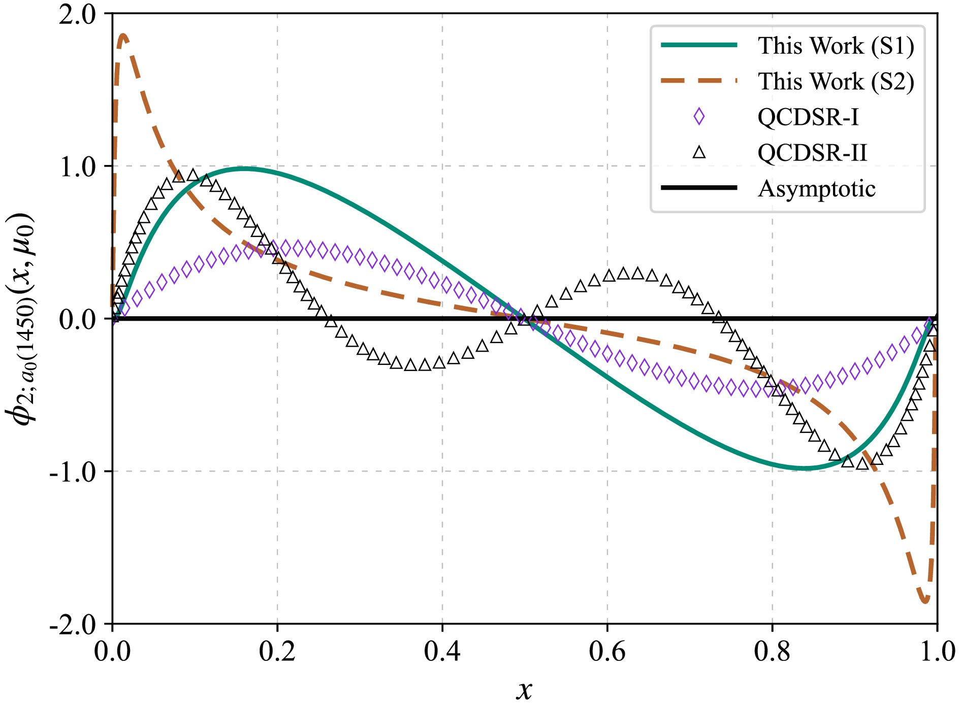
Figure 2. (color online) Behavior of twist-2 LCDAs for
$ a_0(1450) $ at$ \mu_0 = 1\; {\rm{GeV}} $ . For comparison, QCDSR-I and QCDSR-II results (I and II in QCDSR [1] correspond to truncations at$ {\cal{N}}=1 $ and$ {\cal{N}}=3 $ , respectively) are also shown.Using the definition in Eq. (22), we calculated the moments
$ \langle\xi^{n}\rangle|_{\mu_0}^{\mathrm{(S1,S2)}} $ with$ n=(1,3,5) $ and the corresponding Gegenbauer moments$ a_n^{(\rm{S1,S2})}(\mu_0) $ . Since the zeroth-order Gegenbauer moment of$ a_0(1450) $ is zero and even-order coefficients are highly suppressed, under the approximation of equal constituent quark masses$ (m_1 =m_2) $ the even-order coefficients vanish. Thus, the twist-2 LCDA of$ a_0(1450) $ is dominated by odd-order Gegenbauer moments.$ \begin{aligned}[b] &\langle\xi^{1} \rangle|^{({\rm{S}}1)}_{\mu_0}=-0.348^{+0.072}_{-0.072}, \; \; \; \langle\xi^{1} \rangle|^{({\rm{S}}2)}_{\mu_0}=-0.348^{+0.072}_{-0.072}, \\ &\langle\xi^{3} \rangle|^{({\rm{S}}1)}_{\mu_0}=-0.160^{+0.033}_{-0.033}, \; \; \; \langle\xi^{3} \rangle|^{({\rm{S}}2)}_{\mu_0}=-0.242^{+0.059}_{-0.060}, \\ &\langle\xi^{5} \rangle|^{({\rm{S}}1)}_{\mu_0}=-0.092^{+0.019}_{-0.019}, \; \; \; \langle\xi^{5} \rangle|^{({\rm{S}}2)}_{\mu_0}=-0.188^{+0.051}_{-0.052}, \\ &a_{1}^{({\rm{S}}1)}(\mu_0)=-0.580^{+0.120}_{-0.120}, \; \; \; a_{1}^{({\rm{S}}2)}(\mu_0)=-0.580^{+0.120}_{-0.120}, \\ &a_{3}^{({\rm{S}}1)}(\mu_0)=-0.057^{+0.011}_{-0.011}, \; \; \; a_{3}^{({\rm{S}}2)}(\mu_0)=-0.488^{+0.148}_{-0.153}, \\ &a_{5}^{({\rm{S}}1)}(\mu_0)=+0.013^{+0.002}_{-0.002}, \; \; \; a_{5}^{({\rm{S}}2)}(\mu_0)=-0.371^{+0.148}_{-0.131}. \end{aligned} $
(26) In addition, we present the
$ \langle\xi^{n} \rangle|^{\mathrm{(S1,S2)}}_{\mu_k} $ moments and the Gegenbauer moments$ a_n^{(\rm{S1,S2})}(\mu_k) $ at the corresponding energy scale$ \mu_{k}=1.4\; {\rm{GeV}} $ .$ \begin{aligned}[b] &\langle\xi^{1} \rangle|^{({\rm{S}}1)}_{\mu_k}=-0.304^{+0.065}_{-0.058}, \; \; \; \langle\xi^{1} \rangle|^{({\rm{S}}2)}_{\mu_k}=-0.249^{+0.065}_{-0.065}, \\ &\langle\xi^{3} \rangle|^{({\rm{S}}1)}_{\mu_k}=-0.137^{+0.029}_{-0.026}, \; \; \; \langle\xi^{3} \rangle|^{({\rm{S}}2)}_{\mu_k}=-0.173^{+0.044}_{-0.045}, \\ &\langle\xi^{5} \rangle|^{({\rm{S}}1)}_{\mu_k}=-0.078^{+0.017}_{-0.014}, \; \; \; \langle\xi^{5} \rangle|^{({\rm{S}}2)}_{\mu_k}=-0.135^{+0.034}_{-0.034}, \\ &a_{1}^{({\rm{S}}1)}(\mu_k)=-0.507^{+0.109}_{-0.096}, \; \; \; a_{1}^{({\rm{S}}2)}(\mu_k)=-0.415^{+0.108}_{-0.108}, \\ &a_{3}^{({\rm{S}}1)}(\mu_k)=-0.035^{+0.006}_{-0.006}, \; \; \; a_{3}^{({\rm{S}}2)}(\mu_k)=-0.348^{+0.085}_{-0.090}, \\ &a_{5}^{({\rm{S}}1)}(\mu_k)=+0.009^{+0.008}_{-0.015}, \; \; \; a_{5}^{({\rm{S}}2)}(\mu_k)=-0.277^{+0.070}_{-0.052}. \end{aligned} $
(27) For
$ n=1,3,5 $ , the moments obtained from the two LCDA schemes generally exhibit a linear relationship: their absolute values decrease as n increases, and the magnitudes from the first scheme are larger. Specifically, at$ n=1 $ , the$ \langle\xi^{1}\rangle|^{({\rm{S}}1/{\rm{S}}2)}_{\mu_0} $ values from the two LCDA schemes are numerically identical, whereas for$ n=3 $ and$ n=5 $ the differences between the moments from the two schemes increase significantly with the order, indicating that the factor$ (2x-1)^n $ in higher-order moments is more sensitive to the value of x. In addition, for the twist-3 LCDA$ \phi_{3;a_0}^{p,\sigma}(x,\mu) $ of the$ a_0(1450) $ , we adopt the Gegenbauer moments at the energy scale$ \mu_{k}=1.4\; {\rm{GeV}} $ as follows [5]:$ \begin{aligned}[b] &a_{2}^{p}(\mu_{k})=0.236 \pm{0.008}, &a_{4}^{p}(\mu_{k})=0.504 \pm{0.159}, \\ &a_{2}^{\sigma}(\mu_{k})=0.009 \pm{0.001}, &a_{4}^{\sigma}(\mu_{k})=0.043 \pm{0.008}, \end{aligned} $
(28) Using the resultant twist-2 and twist-3 LCDAs of the
$ a_0(1450) $ state, we can further calculate the$ D\to a_0(1450) $ TFFs. To determine the continuum threshold and Borel windows, we adopt two criteria: (1) the contributions from the continuum and higher excited states are less than 30%; (2) the dependence of the form factors on the Borel parameter is weak. Accordingly, we set the values of$ s_0 $ and$ M^2 $ to$ 2.9 \pm0.05 {\; {\rm{GeV}}}^2 $ and$ 15 \pm0.05 {\; {\rm{GeV}}}^2 $ for$ f_+^{({\rm{S}}1,{\rm{S}}2)}(q^2) $ , and$ 5 \pm0.05 {\; {\rm{GeV}}}^2 $ and$ 5 \pm0.05 {\; {\rm{GeV}}}^2 $ for$ f_- (q^2) $ , respectively. We then obtain the numerical results for the$ D \to a_0(1450) $ transition TFFs in the large-recoil region, which are presented in Table 1. At the same time, to intuitively demonstrate the stability of the sum rule with respect to$ M^2 $ , we plot the curves of the TFFs as functions of the Borel parameter$ M^2 $ in Fig. 3, where$ q^2=0\; {\rm{GeV}}^2 $ . It can be seen that the TFFs exhibit clear stability against variations of$ M^2 $ within the chosen interval. We also present the predictions of QCDSR-II [1], CLFQM [44], RQM [45], and LCSR [46] for comparison. We find that our result$ f_+^{ (\mathrm{S2})}(0) $ is closest to the RQM prediction. The QCDSR-II [1] prediction also lies within our uncertainty range.$ f_+(0) $ $ f_{-}(0) $ This work (S1) $ 0.836_{-0.119}^{+0.116} $ $ 0.630_{-0.077}^{+0.078} $ This work (S2) $ 0.767_{-0.105}^{+0.106} $ $ 0.630_{-0.077}^{+0.078} $ QCDSR-II [1] $ 0.691 $ −− CLFQM [44] $ 0.51_{+0.01-0.02}^{-0.01+0.01} $ −− RQM [45] $ 0.719 $ $ -1.391 $ LCSR [46] $ 0.94_{-0.03}^{+0.02} $ $ -0.94_{-0.03}^{+0.02} $ 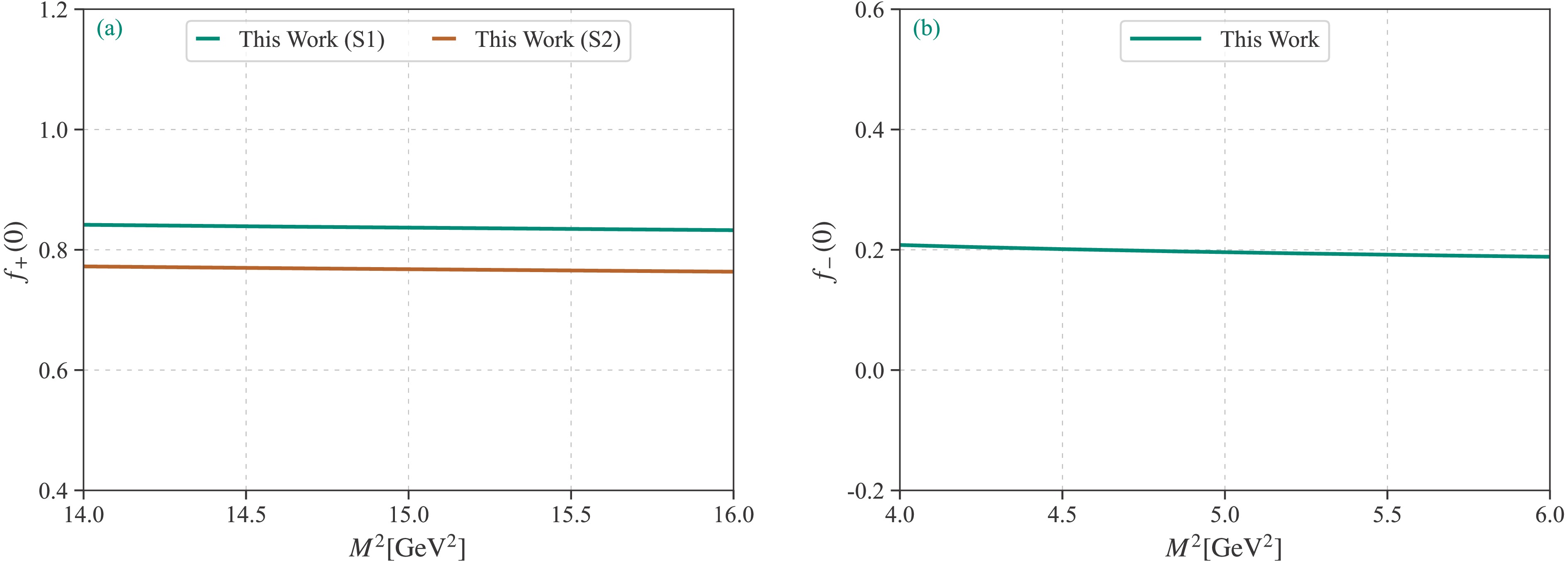
Figure 3. (color online) Dependence of
$ f_+^{({\rm{S}}1,{\rm{S}}2)}(0) $ and$ f_-(0) $ on the Borel parameter$ M^2 $ at$ q^2=0\; {\rm{GeV}}^2 $ .Our result for
$ f_-(0) $ differs from those reported by QCDSR-II [1] and CLFQM [44]. This discrepancy can be attributed to differences in methods and input parameters. In particular, the substantial discrepancy with the LCSR [46] prediction stems from differences in our choice of the twist-2 LCDA model and the formulation of the TFFs. Currently, theoretical predictions for$ f_-(0) $ at the large-recoil point still vary across groups. Moreover, examining the overall behavior of the TFFs can help assess the reliability of the numerical results.Since the LCSR approach is primarily applicable to the low- and intermediate-
$ q^2 $ regions, we therefore adopt the simplified series expansion (SSE) to fit the complex analytical results and extrapolate them to the entire$ q^2 $ region, thereby obtaining a reasonable behavior of the TFF for the transition process$ D \to a_0(1450) $ over the full physical range, i.e.,$ 0 \leq q^2 \leq ( m_D-m_{a_0(1450)})^2 $ . The SSE is a rapidly convergent series in the$ z(t) $ expansion, which can be written as follows [73]:$ f_i(q^2) = P_i(q^2) \sum\limits_{k=0,1,2} a_k^i[z(q^2)-z(0)]^k, $
(29) where
$ f_i(q^2) $ denotes the$ D \to a_0(1450) $ TFFs,$ a_k^i $ are the coefficients, and$ P_i(q^2) = \big(1-{q^2}/{m_{R,i}^2} \big)^{-1} $ ,$ z(t) = (\sqrt{t_+-t}- \sqrt{t_+-t_0})/({\sqrt{t_+-t}+\sqrt{t_+-t_0}}) $ , with$ t_+=(m_D - m_{a_0(1450)})^2 $ ,$ t_{0}=t_+(1-\sqrt{1-(t_{-})/(t_+)}) $ .$ P_i(q^2) $ is a simple pole associated with the lowest-lying resonance in the spectrum and is used to account for the low-lying resonance;$ m_{R,i} $ is the D-meson resonance mass. The relevant low-lying D-meson resonances with the appropriate$ J^P $ quantum numbers are$ m_{D^*}(2007)^0 $ and$ m_{D^*_0}(2300) $ . The free parameters$ a_{1}^i $ and$ a_{2}^i $ are determined to minimize the TFF goodness-of-fit measure Δ. Conventionally, we require Δ < 1%, and we use Δ to quantify the extrapolation quality. We also present the TFF fit parameters in Table 2.$ f_+ (q^2) $ $ f_{-} (q^2) $ $ m_{R,i} $ $ 2.00685 $ $ 2.343 $ $ a_1^{(\mathrm{S1})} $ $ -7.418 $ $ -12.430 $ $ a_2^{(\mathrm{S1})} $ $ 145.839 $ $ 275.236 $ $ \Delta^{(\mathrm{S1})} $ $ 0.117\times 10^{-3} $ $ 0.219\times 10^{-3} $ $ m_{R,i} $ $ 2.00685 $ $ 2.343 $ $ a_1^{(\mathrm{S2})} $ $ -5.077 $ $ -12.430 $ $ a_2^{(\mathrm{S2})} $ $ 146.277 $ $ 275.236 $ $ \Delta^{(\mathrm{S2})} $ $ 0.132\times 10^{-3} $ $ 0.219\times 10^{-3} $ Table 2. Within two LCDA schemes, the masses of the D-meson and its resonances, the fit parameters
$ a_i $ with$ i=(1,2) $ , and the goodness of fit Δ for the form factors$ f_{\pm}^{({\rm{S}}1,{\rm{S}}2)} (q^2) $ are presented, with all input parameters fixed at their central values.After extrapolating the
$ D \to a_0(1450) $ TFFs over the entire physical$ q^2 $ region, the behaviors of$ f_+^{ (\rm{S1,S2})}(q^2) $ and$ f_{-} (q^2) $ are shown in Fig. 4, where$ f_+^{ (\rm{S1,S2})}(q^2) $ corresponds to the two types of twist-2 LCDAs for the$ a_0(1450) $ state. The behavior of$ f_+^{ (\mathrm{S1,S2})}(q^2) $ shows a slow increase within uncertainties across the entire$ q^2 $ region. This is in good agreement with predictions from QCDSR-II [1] and RQM [45], supporting the reliability of our results. For$ f_{-} (q^2) $ , since its expression does not include contributions from the twist-2 LCDA, different twist-2 LCDA schemes have no impact on$ f_{-} (q^2) $ .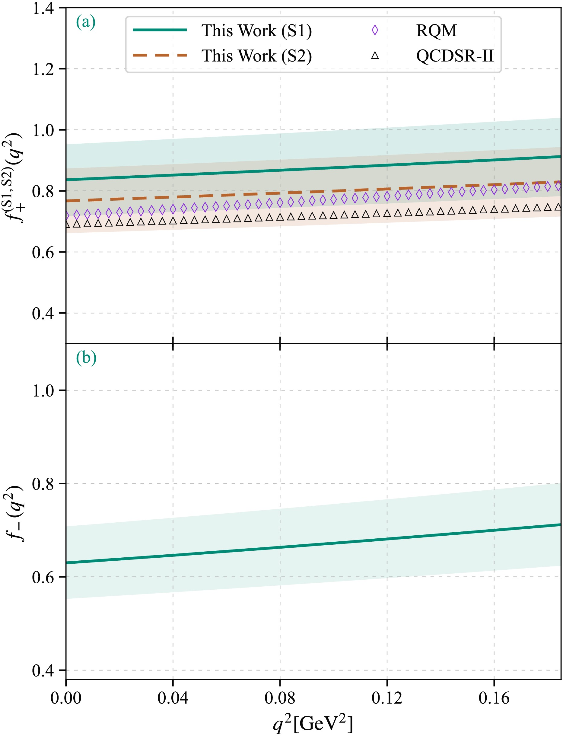
Furthermore, the distribution of differential decay width with respect to angle
$ \cos\theta_\ell $ , i.e.${{\rm d}\Gamma}/{{\rm d}\cos\theta_\ell }$ at the point$ q^2=10^{-5}\; {\rm{GeV}}^2 $ in the region$ \cos\theta_\ell \in[-1,1] $ are shown in Fig. 5. The results show that${{\rm d}\Gamma}/{{\rm d}\cos\theta_\ell }$ exhibits a quadratic dependence on$ \cos\theta_\ell $ , with coefficients primarily determined by the TFFs$ f_+^{({\rm{S}}1,{\rm{S}}2)}(q^2) $ ,$ f_- (q^2) $ and lepton mass$ m_\ell $ . For decay channel$ D^0\to a_0(1450)^- \mu^+\nu_{\mu} $ and$ D^-\to a_0(1450)^0 \mu^-\bar{\nu}_{\mu} $ , the angular distribution increases monotonically with$ \cos\theta_\ell $ and shows a nonzero intercept at the endpoints$ \cos\theta_\ell = \pm 1 $ . This occurs because the angular distribution contains a term linear in$ \cos\theta_\ell $ , which is proportional to$ {m_\ell ^2}/{q^2} $ , leading to a finite value of${{\rm d}\Gamma}/{{\rm d}\cos\theta_\ell }$ at the endpoints when$ q^2=10^{-5}\; {\rm{GeV}}^2 $ . In contrast, for decay channel$ D^0\to a_0(1450)^- e^+\nu_{e} $ and$ D^-\to a_0(1450)^0 e^- \bar{\nu}_{e} $ , the extremely small electron mass ($ m_e \approx 0.5 \rm\; {MeV} $ ) makes angular distribution over$ \cos\theta_\ell \in [-1,1] $ nearly a symmetric parabola. These results demonstrate that the lepton mass has an important impact on the decay angular distribution in the low$ q^2 $ -region.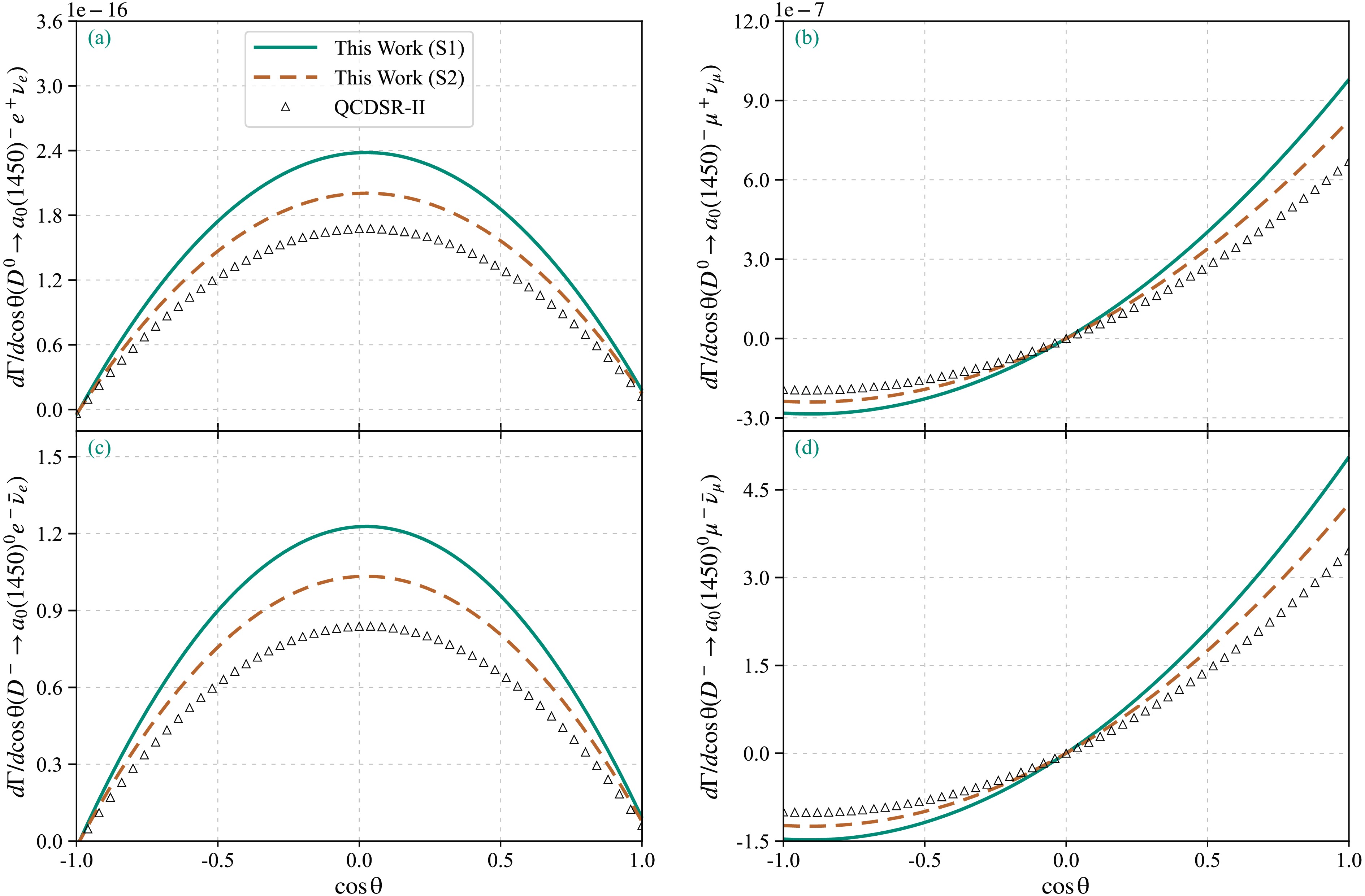
Figure 5. (color online) Angular distribution of
${{\rm d}\Gamma}/{{\rm d}\cos\theta}$ as a function of$ \cos\theta $ for the decay channels$ D^0 \to a_0(1450)^- \ell^+ \nu_\ell $ and$ D^- \to a_0(1450)^0 \ell^- \bar{\nu}_\ell $ , with$ \ell=(e,\mu) $ , at$ q^2=10^{-5}\; {\rm{GeV}}^2 $ . For comparison, the predictions of QCDSR-II [1] are also shown.As a further step, the decay widths and branching fractions for semileptonic
$ D \to a_0(1450) \ell \nu_{\ell} $ decay can be calculated. By taking the CKM matrix element$ |V_{cd}|= 0.221 \pm{0.008} $ from the PDG [16], we obtain the differential decay widths for$ D \to a_0(1450) \ell \nu_{\ell} $ with$ \ell=(e,\mu) $ . Their behaviors are shown in Fig. 6, together with the QCDSR-II prediction [1] for comparison. Since the kinematic$ q^2 $ -region of$ D \to a_0(1450) \ell \nu_\ell $ decay is much smaller than that of$ B \to a_0(1450) \ell \nu_{\ell} $ decay, we separately consider the differential decay widths for electron and muon channels. It can be seen from Fig. 6 that the behavioral trends of our predicted differential decay widths for electrons and muons under two LCDA schemes are basically consistent, though there exist slight differences in numerical results. Compared with the first scheme, the second scheme gives smaller numerical results. This is because the TFF$ f^{ (\rm{S2})}_+(q^2) $ obtained in second scheme is slightly lower than$ f^{ (\rm{S1})}_+(q^2) $ from the first scheme. Therefore, under the same threshold parameter$ s_0 $ and Borel window$ M^2 $ , the differential decay widths for the electron and muon channels in second scheme$ f^{(\rm{S2})}_+(q^2) $ are also smaller.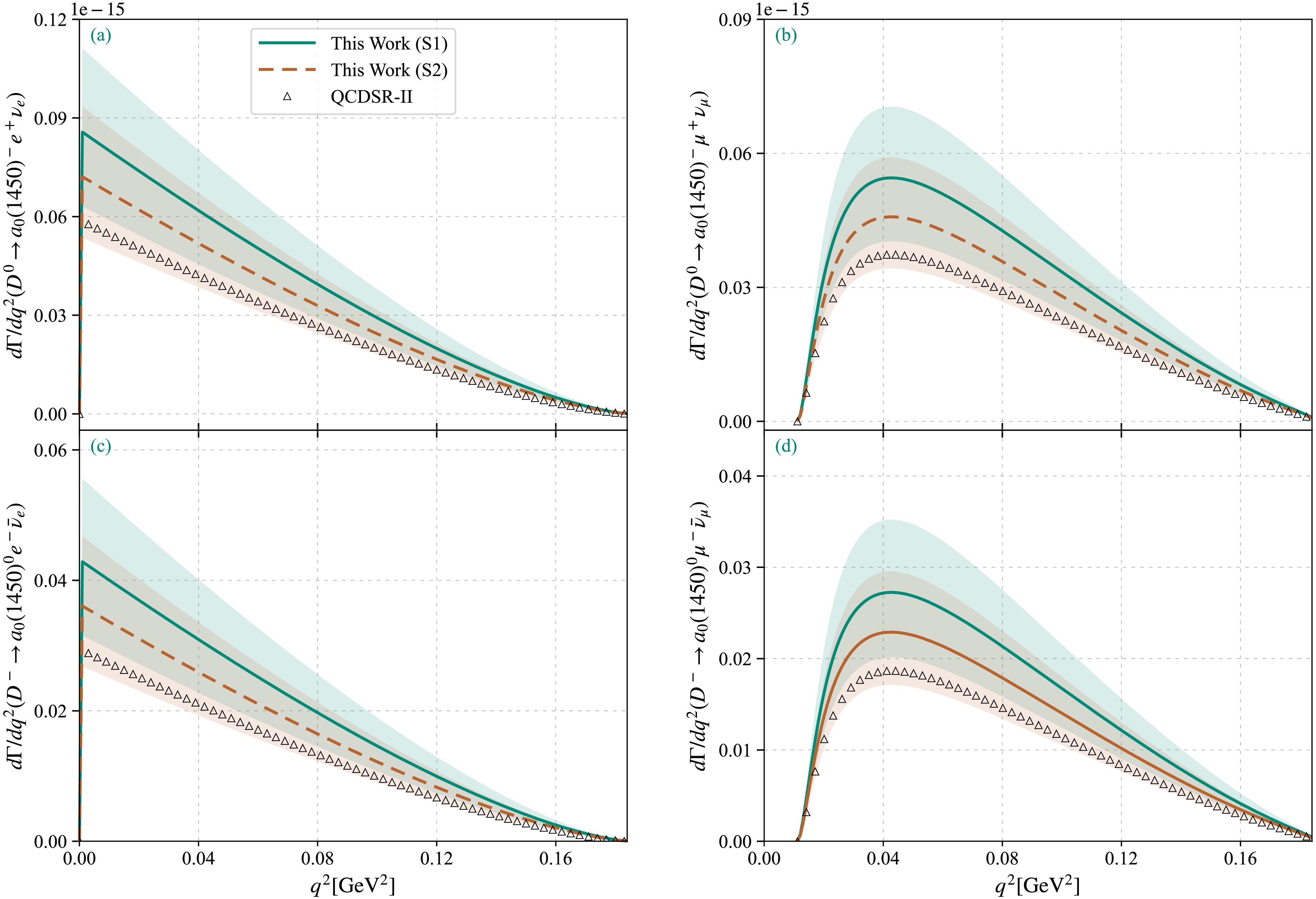
Figure 6. (color online) Decay widths for the semileptonic decay channels
$D^0 \to a_0(1450)^- \ell^+ \nu_\ell$ and$D^- \to a_0(1450)^0 \ell^- \bar{\nu}_\ell$ , with$\ell=(e,\mu)$ , are presented. Predictions from QCDSR-II [1] are included for comparison. Shaded bands indicate the corresponding uncertainties.After taking the lifetimes of
$ D^0 $ and$ D^- $ mesons from the PDG, namely$ \tau_{D^0}=(0.410 \pm{0.001}) $ ps and$ \tau_{D^-}= (1.033\pm{0.005}) $ ps, we also calculated the branching fractions of$ D^0 \to a_0(1450)^{-} \ell^{+} \nu_\ell $ and$ D^- \to a_0(1450)^{0} \ell^{-} \bar{\nu}_\ell $ with$ (\ell= e,\mu) $ . The specific calculation results are listed in Table 3. It can be observed that branching fractions for all decay channels are of the order$ 10^{-6} $ , consistent with results reported by theoretical groups using LCSR [46] and CLFQM [74].$ D^0\to a_0(1450)^- e^+\nu_{e} $ $ D^0\to a_0(1450)^- \mu^+\nu_{\mu} $ $ D^-\to a_0(1450)^0 e^-\bar{\nu}_{e} $ $ D^-\to a_0(1450)^0 \mu^-\bar{\nu}_{\mu} $ This work (S1) $ 4.16^{+1.23}_{-1.10} $ $ 1.91^{+2.27}_{-0.47} $ $ 5.24^{+1.57}_{-1.38} $ $ 2.41^{+2.86}_{-0.59} $ This work (S2) $ 3.48^{+1.03}_{-0.89} $ $ 1.91^{+1.27}_{-0.26} $ $ 4.39^{+1.29}_{-1.12} $ $ 2.41^{+2.01}_{-0.13} $ QCDSR-II [1] $ 2.83 $ $ 1.92 $ $ 3.56 $ $ 2.43 $ LCSR [46] $ 3.14 $ $ 2.01 $ $ 4.28 $ $ 2.76 $ CLFQM [74] −− −− $ 5.4^{+0.05}_{-0.05} $ $ 3.8^{+0.03}_{-0.03} $ Table 3. (color online) Branching fractions (in units of
$ 10^{-6} $ ) for the decay channels$ D^0 \to a_0(1450)^- \ell^+ \nu_\ell $ and$ D^- \to a_0(1450)^0 \ell^- \bar{\nu}_\ell $ , with$ \ell=(e,\mu) $ , are presented with uncertainties for two twist-2 LCDA schemes; predictions from LCSR [46], QCDSR-II [1], and CLFQM [74] are provided for comparison.For the decay channels
$ D^- \to a_0(1450)^{0} e^{-}\bar{\nu}_e $ and$ D^0 \to a_0(1450)^{-} e^{+}\nu_e $ , the numerical results obtained with the two LCDA schemes agree better with LCSR, while they deviate from the CLFQM predictions for$ D^- \to a_0(1450)^{0} e^{-}\bar{\nu}_e $ and$ D^- \to a_0(1450)^{0} \mu^{-}\bar{\nu}_\mu $ . Notably, the central values of the branching fractions for$ D^0 \to a_0(1450)^{-}\mu^{+} \nu_{\mu} $ and$ D^- \to a_0(1450)^{0} \mu^{-}\bar{\nu}_{\mu} $ obtained with the two LCDA schemes and QCDSR-II [1] are identical, differing only marginally in their theoretical uncertainties. Furthermore, the central values from both LCSR and CLFQM lie within our allowed uncertainty range.Finally, we calculated three angular observables for the semileptonic decay
$ D\to a_0(1450) \ell \nu_{\ell} $ : the forward-backward asymmetry$ {\cal{A}}_{\rm{FB}}(q^2) $ , the lepton polarization asymmetry$ {\cal{A}}_{\lambda_\ell} $ , and the$ q^2 $ -differential flat term$ {\cal{F}}_{\rm{H}}(q^2) $ . Since the integrated results for$ D^0 \to a_0(1450)^- \ell^+ \nu_{\ell} $ and$ D^- \to a_0(1450)^0 \ell^- \bar{\nu}_\ell $ decay channels are almost identical, we present only the results for$ D^0 \to a_0(1450)^- \ell^+ \nu_{\ell} $ here. As shown in Table 4, the three angular observables calculated using two twist-2 LCDA schemes yield very similar results, with only slight differences. The integrated$ {\cal{A}}_{\rm{FB}} $ for the electron channel is very small ($ m_{e} \approx 0.5 $ MeV), consistent with the fact that, in weak interactions, helicity suppression is strongly mass dependent and the electron mass is nearly zero. The mass of the muon ($ m_{\mu} \approx 105.7\; {\rm{MeV}} $ ) is comparatively large, so a slight difference in the numerical value of$ {\cal{A}}_{\rm{FB}}(q^2) $ between the two LCDA schemes is observed. In addition,$ {\cal{A}}_{\lambda_\ell}(q^2) $ and$ {\cal{F}}_{\rm{H}}(q^2) $ exhibit clearly different behaviors. Overall,$ {\cal{A}}_{\rm{FB}}(q^2) $ and$ {\cal{F}}_{\rm{H}}(q^2) $ are proportional to the square of the lepton mass, whereas$ {\cal{A}}_{\lambda_\ell}(q^2) $ is inversely proportional to the lepton mass.This work (S1) This work (S2) $ {\cal{A}}_{\rm{FB}}^{D^0 \to a_0(1450)^- e^+ \nu_{e}}(10^{-6}) $ $ 5.46^{+2.54}_{-1.90} $ $ 5.47^{+2.47}_{-1.89} $ $ {\cal{A}}_{\rm{FB}}^{D^0 \to a_0(1450)^-\mu^+ \nu_{\mu}}(10^{-2}) $ $ 3.66^{+1.67}_{-1.26} $ $ 3.66^{+1.62}_{-1.23} $ $ {\cal{A}}_{\lambda \ell}^{D^0 \to a_0(1450)^- e^+ \nu_{e}}(10^{-1}) $ $ 0.18^{+0.31}_{-0.31} $ $ 0.18^{+0.36}_{-0.36} $ $ {\cal{A}}_{\lambda \ell}^{D^0 \to a_0(1450)^-\mu^+ \nu_{\mu}}(10^{-2}) $ $ 0.02^{+0.05}_{-0.06} $ $ 0.02^{+0.05}_{-0.06} $ $ {\cal{F}}_{\rm{H}}^{D^0 \to a_0(1450)^- e^+ \nu_{e}}(10^{-5}) $ $ 1.60^{+0.73}_{-0.54} $ $ 1.60^{+0.71}_{-0.54} $ $ {\cal{F}}_{\rm{H}}^{D^0 \to a_0(1450)^-\mu^+ \nu_{\mu}}(10^{-2}) $ $ 9.03^{+4.07}_{-3.06} $ $ 9.06^{+3.95}_{-3.00} $ Table 4. Integrated results for three angular observables in the semileptonic decay
$ D^0 \to a_0(1450)^- \ell^+ \nu_\ell $ , with$ \ell=(e,\mu) $ , evaluated using two twist-2 LCDA schemes, are presented. -
For numerical calculations, we provide the following input parameters: the meson masses
$ m_{D^0}=1864.84\pm0.05\; {\rm{MeV}} $ ,$ m_{D^-}=1869.66\pm0.05\; {\rm{MeV}} $ , and$ m_{a_0(1450)}=1439\pm34\; {\rm{MeV}} $ ; the quark masses$ m_c(\bar m_c)=1273\pm20\; {\rm{MeV}} $ ,$ m_d=4.67^{+0.48}_{-0.17}\; {\rm{MeV}} $ , and$ m_u=2.16\pm0.07\; {\rm{MeV}} $ at$ \mu=2\; {\rm{GeV}} $ . The decay constants are$ f_D=208.4\pm1.5\; {\rm{MeV}} $ [70] and$ \bar{f}_{a_0(1450)}=460\pm50\; {\rm{MeV}} $ at$ \mu_0 = 1\ {\rm{GeV}} $ [1]. For the$ D\to a_0(1450) $ transition, we also use the corresponding energy scale:$ \mu_{k} = \sqrt{m_D^2 - m_c^2} \simeq 1.4\ {\rm{GeV}} $ . As discussed in Section II regarding the twist-2 LCDA model parameters, we adopt$ a_1(\mu_0)=-0.58\pm0.12 $ and$ \langle {\bf{k}}_{\perp}^2\rangle^{1/2}=0.37\; {\rm{GeV}} $ for the first scheme. For the second scheme, an additional condition$ a_3(\mu_0)=-0.49\pm0.15 $ is imposed [1]. Based on these choices, the LCDAs of$ a_{0}(1450) $ are then fixed. In addition, we use renormalization group evolution (RGE) to run these parameters to the corresponding energy scale$ \mu_k $ [71, 72].At the initial energy scale
$ \mu_0=1\; {\rm{GeV}} $ , we present the model parameters of the two LCDA schemes for the light scalar state$ a_0(1450) $ , based on the typical values of$ a_{1}(\mu_0) $ and$ \langle {\bf{k}}_{\perp}^2\rangle^{1/2} $ .$ \begin{aligned}[b] & A^{({\rm{S}}1)}=390.35, \quad \beta^{({\rm{S}}1)}=-0.724; \\ & A^{({\rm{S}}2)}=-17.987,\quad \beta^{({\rm{S}}2)}=1.424, \quad \alpha^{({\rm{S}}2)} =-0.951. \end{aligned} $
(25) The corresponding LCDA behavior is presented in Fig. 2. It can be seen that our predictions for the twist-2 LCDA in both schemes exhibit antisymmetric behavior, consistent with the results from QCDSRs. Our S1 result is also identical in behavior to QCDSR-I [1]. However, some differences remain, likely due to the different models employed: we construct the twist-2 LCDA using the LCHO model, whereas QCDSRs adopt a Gegenbauer-moment polynomial expansion. Furthermore, in the calculation of subsequent observables, we find that the numerical results of QCDSR-I and QCDSR-II are almost identical. Thus, in the following discussion, we adopt only QCDSR-II for analysis.
Figure 2. (color online) Behavior of twist-2 LCDAs for
$ a_0(1450) $ at$ \mu_0 = 1\; {\rm{GeV}} $ . For comparison, QCDSR-I and QCDSR-II results (I and II in QCDSR [1] correspond to truncations at$ {\cal{N}}=1 $ and$ {\cal{N}}=3 $ , respectively) are also shown.Using the definition in Eq. (22), we calculated the moments
$ \langle\xi^{n}\rangle|_{\mu_0}^{\mathrm{(S1,S2)}} $ with$ n=(1,3,5) $ and the corresponding Gegenbauer moments$ a_n^{(\rm{S1,S2})}(\mu_0) $ . Since the zeroth-order Gegenbauer moment of$ a_0(1450) $ is zero and even-order coefficients are highly suppressed, under the approximation of equal constituent quark masses$ (m_1 =m_2) $ the even-order coefficients vanish. Thus, the twist-2 LCDA of$ a_0(1450) $ is dominated by odd-order Gegenbauer moments.$ \begin{aligned}[b] &\langle\xi^{1} \rangle|^{({\rm{S}}1)}_{\mu_0}=-0.348^{+0.072}_{-0.072}, \; \; \; \langle\xi^{1} \rangle|^{({\rm{S}}2)}_{\mu_0}=-0.348^{+0.072}_{-0.072}, \\ &\langle\xi^{3} \rangle|^{({\rm{S}}1)}_{\mu_0}=-0.160^{+0.033}_{-0.033}, \; \; \; \langle\xi^{3} \rangle|^{({\rm{S}}2)}_{\mu_0}=-0.242^{+0.059}_{-0.060}, \\ &\langle\xi^{5} \rangle|^{({\rm{S}}1)}_{\mu_0}=-0.092^{+0.019}_{-0.019}, \; \; \; \langle\xi^{5} \rangle|^{({\rm{S}}2)}_{\mu_0}=-0.188^{+0.051}_{-0.052}, \\ &a_{1}^{({\rm{S}}1)}(\mu_0)=-0.580^{+0.120}_{-0.120}, \; \; \; \quad a_{1}^{({\rm{S}}2)}(\mu_0)=-0.580^{+0.120}_{-0.120}, \\ &a_{3}^{({\rm{S}}1)}(\mu_0)=-0.057^{+0.011}_{-0.011}, \; \; \; \quad a_{3}^{({\rm{S}}2)}(\mu_0)=-0.488^{+0.148}_{-0.153}, \\ &a_{5}^{({\rm{S}}1)}(\mu_0)=+0.013^{+0.002}_{-0.002}, \; \; \; \quad a_{5}^{({\rm{S}}2)}(\mu_0)=-0.371^{+0.148}_{-0.131}. \end{aligned} $
(26) In addition, we present the
$ \langle\xi^{n} \rangle|^{\mathrm{(S1,S2)}}_{\mu_k} $ moments and the Gegenbauer moments$ a_n^{(\rm{S1,S2})}(\mu_k) $ at the corresponding energy scale$ \mu_{k}=1.4\; {\rm{GeV}} $ .$ \begin{aligned}[b] &\langle\xi^{1} \rangle|^{({\rm{S}}1)}_{\mu_k}=-0.304^{+0.065}_{-0.058}, \; \; \; \langle\xi^{1} \rangle|^{({\rm{S}}2)}_{\mu_k}=-0.249^{+0.065}_{-0.065}, \\ &\langle\xi^{3} \rangle|^{({\rm{S}}1)}_{\mu_k}=-0.137^{+0.029}_{-0.026}, \; \; \; \langle\xi^{3} \rangle|^{({\rm{S}}2)}_{\mu_k}=-0.173^{+0.044}_{-0.045}, \\ &\langle\xi^{5} \rangle|^{({\rm{S}}1)}_{\mu_k}=-0.078^{+0.017}_{-0.014}, \; \; \; \langle\xi^{5} \rangle|^{({\rm{S}}2)}_{\mu_k}=-0.135^{+0.034}_{-0.034}, \\ &a_{1}^{({\rm{S}}1)}(\mu_k)=-0.507^{+0.109}_{-0.096}, \; \; \; \quad a_{1}^{({\rm{S}}2)}(\mu_k)=-0.415^{+0.108}_{-0.108}, \\ &a_{3}^{({\rm{S}}1)}(\mu_k)=-0.035^{+0.006}_{-0.006}, \; \; \; \quad a_{3}^{({\rm{S}}2)}(\mu_k)=-0.348^{+0.085}_{-0.090}, \\ &a_{5}^{({\rm{S}}1)}(\mu_k)=+0.009^{+0.008}_{-0.015}, \; \; \; \quad a_{5}^{({\rm{S}}2)}(\mu_k)=-0.277^{+0.070}_{-0.052}. \end{aligned} $
(27) For
$ n=1,3,5 $ , the moments obtained from the two LCDA schemes generally exhibit a linear relationship: their absolute values decrease as n increases, and the magnitudes from the first scheme are larger. Specifically, at$ n=1 $ , the$ \langle\xi^{1}\rangle|^{({\rm{S}}1/{\rm{S}}2)}_{\mu_0} $ values from the two LCDA schemes are numerically identical, whereas for$ n=3 $ and$ n=5 $ the differences between the moments from the two schemes increase significantly with the order, indicating that the factor$ (2x-1)^n $ in higher-order moments is more sensitive to the value of x. In addition, for the twist-3 LCDA$ \phi_{3;a_0}^{p,\sigma}(x,\mu) $ of the$ a_0(1450) $ , we adopt the Gegenbauer moments at the energy scale$ \mu_{k}=1.4\; {\rm{GeV}} $ as follows [5]:$ \begin{aligned}[b] &a_{2}^{p}(\mu_{k})=0.236 \pm{0.008}, &a_{4}^{p}(\mu_{k})=0.504 \pm{0.159}, \\ &a_{2}^{\sigma}(\mu_{k})=0.009 \pm{0.001}, &a_{4}^{\sigma}(\mu_{k})=0.043 \pm{0.008}, \end{aligned} $
(28) Using the resultant twist-2 and twist-3 LCDAs of the
$ a_0(1450) $ state, we can further calculate the$ D\to a_0(1450) $ TFFs. To determine the continuum threshold and Borel windows, we adopt two criteria: (1) the contributions from the continuum and higher excited states are less than 30%; (2) the dependence of the form factors on the Borel parameter is weak. Accordingly, we set the values of$ s_0 $ and$ M^2 $ to$ 2.9 \pm0.05 {\; {\rm{GeV}}}^2 $ and$ 15 \pm0.05 {\; {\rm{GeV}}}^2 $ for$ f_+^{({\rm{S}}1,{\rm{S}}2)}(q^2) $ , and$ 5 \pm0.05 {\; {\rm{GeV}}}^2 $ and$ 5 \pm0.05 {\; {\rm{GeV}}}^2 $ for$ f_- (q^2) $ , respectively. We then obtain the numerical results for the$ D \to a_0(1450) $ transition TFFs in the large-recoil region, which are presented in Table 1. At the same time, to intuitively demonstrate the stability of the sum rule with respect to$ M^2 $ , we plot the curves of the TFFs as functions of the Borel parameter$ M^2 $ in Fig. 3, where$ q^2=0\; {\rm{GeV}}^2 $ . It can be seen that the TFFs exhibit clear stability against variations of$ M^2 $ within the chosen interval. We also present the predictions of QCDSR-II [1], CLFQM [44], RQM [45], and LCSR [46] for comparison. We find that our result$ f_+^{ (\mathrm{S2})}(0) $ is closest to the RQM prediction. The QCDSR-II [1] prediction also lies within our uncertainty range.$ f_+(0) $ $ f_{-}(0) $ This work (S1) $ 0.836_{-0.119}^{+0.116} $ $ 0.630_{-0.077}^{+0.078} $ This work (S2) $ 0.767_{-0.105}^{+0.106} $ $ 0.630_{-0.077}^{+0.078} $ QCDSR-II [1] $ 0.691 $ −− CLFQM [44] $ 0.51_{+0.01-0.02}^{-0.01+0.01} $ −− RQM [45] $ 0.719 $ $ -1.391 $ LCSR [46] $ 0.94_{-0.03}^{+0.02} $ $ -0.94_{-0.03}^{+0.02} $
Figure 3. (color online) Dependence of
$ f_+^{({\rm{S}}1,{\rm{S}}2)}(0) $ and$ f_-(0) $ on the Borel parameter$ M^2 $ at$ q^2=0\; {\rm{GeV}}^2 $ .Our result for
$ f_-(0) $ differs from those reported by QCDSR-II [1] and CLFQM [44]. This discrepancy can be attributed to differences in methods and input parameters. In particular, the substantial discrepancy with the LCSR [46] prediction stems from differences in our choice of the twist-2 LCDA model and the formulation of the TFFs. Currently, theoretical predictions for$ f_-(0) $ at the large-recoil point still vary across groups. Moreover, examining the overall behavior of the TFFs can help assess the reliability of the numerical results.Since the LCSR approach is primarily applicable to the low- and intermediate-
$ q^2 $ regions, we therefore adopt the simplified series expansion (SSE) to fit the complex analytical results and extrapolate them to the entire$ q^2 $ region, thereby obtaining a reasonable behavior of the TFF for the transition process$ D \to a_0(1450) $ over the full physical range, i.e.,$ 0 \leq q^2 \leq ( m_D-m_{a_0(1450)})^2 $ . The SSE is a rapidly convergent series in the$ z(t) $ expansion, which can be written as follows [73]:$ f_i(q^2) = P_i(q^2) \sum\limits_{k=0,1,2} a_k^i[z(q^2)-z(0)]^k, $
(29) where
$ f_i(q^2) $ denotes the$ D \to a_0(1450) $ TFFs,$ a_k^i $ are the coefficients, and$ P_i(q^2) = \big(1-{q^2}/{m_{R,i}^2} \big)^{-1} $ ,$ z(t) = (\sqrt{t_+-t}- \sqrt{t_+-t_0})/({\sqrt{t_+-t}+\sqrt{t_+-t_0}}) $ , with$ t_+=(m_D - m_{a_0(1450)})^2 $ ,$ t_{0}=t_+(1-\sqrt{1-(t_{-})/(t_+)}) $ .$ P_i(q^2) $ is a simple pole associated with the lowest-lying resonance in the spectrum and is used to account for the low-lying resonance;$ m_{R,i} $ is the D-meson resonance mass. The relevant low-lying D-meson resonances with the appropriate$ J^P $ quantum numbers are$ m_{D^*}(2007)^0 $ and$ m_{D^*_0}(2300) $ . The free parameters$ a_{1}^i $ and$ a_{2}^i $ are determined to minimize the TFF goodness-of-fit measure Δ. Conventionally, we require Δ < 1%, and we use Δ to quantify the extrapolation quality. We also present the TFF fit parameters in Table 2.$ f_+ (q^2) $ $ f_{-} (q^2) $ $ m_{R,i} $ $ 2.00685 $ $ 2.343 $ $ a_1^{(\mathrm{S1})} $ $ -7.418 $ $ -12.430 $ $ a_2^{(\mathrm{S1})} $ $ 145.839 $ $ 275.236 $ $ \Delta^{(\mathrm{S1})} $ $ 0.117\times 10^{-3} $ $ 0.219\times 10^{-3} $ $ m_{R,i} $ $ 2.00685 $ $ 2.343 $ $ a_1^{(\mathrm{S2})} $ $ -5.077 $ $ -12.430 $ $ a_2^{(\mathrm{S2})} $ $ 146.277 $ $ 275.236 $ $ \Delta^{(\mathrm{S2})} $ $ 0.132\times 10^{-3} $ $ 0.219\times 10^{-3} $ Table 2. Within two LCDA schemes, the masses of the D-meson and its resonances, the fit parameters
$ a_i $ with$ i=(1,2) $ , and the goodness of fit Δ for the form factors$ f_{\pm}^{({\rm{S}}1,{\rm{S}}2)} (q^2) $ are presented, with all input parameters fixed at their central values.After extrapolating the
$ D \to a_0(1450) $ TFFs over the entire physical$ q^2 $ region, the behaviors of$ f_+^{ (\rm{S1,S2})}(q^2) $ and$ f_{-} (q^2) $ are shown in Fig. 4, where$ f_+^{ (\rm{S1,S2})}(q^2) $ corresponds to the two types of twist-2 LCDAs for the$ a_0(1450) $ state. The behavior of$ f_+^{ (\mathrm{S1,S2})}(q^2) $ shows a slow increase within uncertainties across the entire$ q^2 $ region. This is in good agreement with predictions from QCDSR-II [1] and RQM [45], supporting the reliability of our results. For$ f_{-} (q^2) $ , since its expression does not include contributions from the twist-2 LCDA, different twist-2 LCDA schemes have no impact on$ f_{-} (q^2) $ .
Furthermore, the distribution of differential decay width with respect to angle
$ \cos\theta_\ell $ , i.e.$ {d\Gamma}/{d\cos\theta_\ell } $ at the point$ q^2=10^{-5}\; {\rm{GeV}}^2 $ in the region$ \cos\theta_\ell \in[-1,1] $ are shown in Fig. 5. The results show that$ {d\Gamma}/{d\cos\theta_\ell } $ exhibits a quadratic dependence on$ \cos\theta_\ell $ , with coefficients primarily determined by the TFFs$ f_+^{({\rm{S}}1,{\rm{S}}2)}(q^2) $ ,$ f_- (q^2) $ and lepton mass$ m_\ell $ . For decay channel$ D^0\to a_0(1450)^- \mu^+\nu_{\mu} $ and$ D^-\to a_0(1450)^0 \mu^-\bar{\nu}_{\mu} $ , the angular distribution increases monotonically with$ \cos\theta_\ell $ and shows a nonzero intercept at the endpoints$ \cos\theta_\ell = \pm 1 $ . This occurs because the angular distribution contains a term linear in$ \cos\theta_\ell $ , which is proportional to$ {m_\ell ^2}/{q^2} $ , leading to a finite value of$ {d\Gamma}/{d\cos\theta_\ell } $ at the endpoints when$ q^2=10^{-5}\; {\rm{GeV}}^2 $ . In contrast, for decay channel$ D^0\to a_0(1450)^- e^+\nu_{e} $ and$ D^-\to a_0(1450)^0 e^- \bar{\nu}_{e} $ , the extremely small electron mass ($ m_e \approx 0.5 \rm\; {MeV} $ ) makes angular distribution over$ \cos\theta_\ell \in[-1,1] $ nearly a symmetric parabola. These results demonstrate that the lepton mass has an important impact on the decay angular distribution in the low$ q^2 $ -region.
Figure 5. (color online) Angular distribution of
$ {d\Gamma}/{d\cos\theta} $ as a function of$ \cos\theta $ for the decay channels$ D^0 \to a_0(1450)^- \ell^+ \nu_\ell $ and$ D^- \to a_0(1450)^0 \ell^- \bar{\nu}_\ell $ , with$ \ell=(e,\mu) $ , at$ q^2=10^{-5}\; {\rm{GeV}}^2 $ . For comparison, the predictions of QCDSR-II [1] are also shown.As a further step, the decay widths and branching fractions for semileptonic
$ D \to a_0(1450) \ell \nu_{\ell} $ decay can be calculated. By taking the CKM matrix element$ |V_{cd}|=0.221 \pm{0.008} $ from the PDG [16], we obtain the differential decay widths for$ D \to a_0(1450) \ell \nu_{\ell} $ with$ \ell=(e,\mu) $ . Their behaviors are shown in Fig. 6, together with the QCDSR-II prediction [1] for comparison. Since the kinematic$ q^2 $ -region of$ D \to a_0(1450) \ell \nu_\ell $ decay is much smaller than that of$ B \to a_0(1450) \ell \nu_{\ell} $ decay, we separately consider the differential decay widths for electron and muon channels. It can be seen from Fig. 6 that the behavioral trends of our predicted differential decay widths for electrons and muons under two LCDA schemes are basically consistent, though there exist slight differences in numerical results. Compared with the first scheme, the second scheme gives smaller numerical results. This is because the TFF$ f^{ (\rm{S2})}_+(q^2) $ obtained in second scheme is slightly lower than$ f^{ (\rm{S1})}_+(q^2) $ from the first scheme. Therefore, under the same threshold parameter$ s_0 $ and Borel window$ M^2 $ , the differential decay widths for the electron and muon channels in second scheme$ f^{(\rm{S2})}_+(q^2) $ are also smaller.
Figure 6. Decay widths for the semileptonic decay channels
$D^0 \to a_0(1450)^- \ell^+ \nu_\ell$ and$D^- \to a_0(1450)^0 \ell^- \bar{\nu}_\ell$ , with$\ell=(e,\mu)$ , are presented. Predictions from QCDSR-II [1] are included for comparison. Shaded bands indicate the corresponding uncertainties.After taking the lifetimes of
$ D^0 $ and$ D^- $ mesons from the PDG, namely$ \tau_{D^0}=(0.410 \pm{0.001}) $ ps and$ \tau_{D^-}=(1.033\pm{0.005}) $ ps, we also calculated the branching fractions of$ D^0 \to a_0(1450)^{-} \ell^{+} \nu_\ell $ and$ D^- \to a_0(1450)^{0} \ell^{-} \bar{\nu}_\ell $ with$ (\ell= e,\mu) $ . The specific calculation results are listed in Table 3. It can be observed that branching fractions for all decay channels are of the order$ 10^{-6} $ , consistent with results reported by theoretical groups using LCSR [46] and CLFQM [74].$ D^0\to a_0(1450)^- e^+\nu_{e} $ $ D^0\to a_0(1450)^- \mu^+\nu_{\mu} $ $ D^-\to a_0(1450)^0 e^-\bar{\nu}_{e} $ $ D^-\to a_0(1450)^0 \mu^-\bar{\nu}_{\mu} $ This work (S1) $ 4.16^{+1.23}_{-1.10} $ $ 1.91^{+2.27}_{-0.47} $ $ 5.24^{+1.57}_{-1.38} $ $ 2.41^{+2.86}_{-0.59} $ This work (S2) $ 3.48^{+1.03}_{-0.89} $ $ 1.91^{+1.27}_{-0.26} $ $ 4.39^{+1.29}_{-1.12} $ $ 2.41^{+2.01}_{-0.13} $ QCDSR-II [1] $ 2.83 $ $ 1.92 $ $ 3.56 $ $ 2.43 $ LCSR [46] $ 3.14 $ $ 2.01 $ $ 4.28 $ $ 2.76 $ CLFQM [74] −− −− $ 5.4^{+0.05}_{-0.05} $ $ 3.8^{+0.03}_{-0.03} $ Table 3. (color online) Branching fractions (in units of
$ 10^{-6} $ ) for the decay channels$ D^0 \to a_0(1450)^- \ell^+ \nu_\ell $ and$ D^- \to a_0(1450)^0 \ell^- \bar{\nu}_\ell $ , with$ \ell=(e,\mu) $ , are presented with uncertainties for two twist-2 LCDA schemes; predictions from LCSR [46], QCDSR-II [1], and CLFQM [74] are provided for comparison.For the decay channels
$ D^- \to a_0(1450)^{0} e^{-}\bar{\nu}_e $ and$ D^0 \to a_0(1450)^{-} e^{+}\nu_e $ , the numerical results obtained with the two LCDA schemes agree better with LCSR, while they deviate from the CLFQM predictions for$ D^- \to a_0(1450)^{0} e^{-}\bar{\nu}_e $ and$ D^- \to a_0(1450)^{0} \mu^{-}\bar{\nu}_\mu $ . Notably, the central values of the branching fractions for$ D^0 \to a_0(1450)^{-}\mu^{+} \nu_{\mu} $ and$ D^- \to a_0(1450)^{0} \mu^{-}\bar{\nu}_{\mu} $ obtained with the two LCDA schemes and QCDSR-II [1] are identical, differing only marginally in their theoretical uncertainties. Furthermore, the central values from both LCSR and CLFQM lie within our allowed uncertainty range.Finally, we calculated three angular observables for the semileptonic decay
$ D\to a_0(1450) \ell \nu_{\ell} $ : the forward-backward asymmetry$ {\cal{A}}_{\rm{FB}}(q^2) $ , the lepton polarization asymmetry$ {\cal{A}}_{\lambda_\ell} $ , and the$ q^2 $ -differential flat term$ {\cal{F}}_{\rm{H}}(q^2) $ . Since the integrated results for$ D^0 \to a_0(1450)^- \ell^+ \nu_{\ell} $ and$ D^- \to a_0(1450)^0 \ell^- \bar{\nu}_\ell $ decay channels are almost identical, we present only the results for$ D^0 \to a_0(1450)^- \ell^+ \nu_{\ell} $ here. As shown in Table 4, the three angular observables calculated using two twist-2 LCDA schemes yield very similar results, with only slight differences. The integrated$ {\cal{A}}_{\rm{FB}} $ for the electron channel is very small ($ m_{e} \approx 0.5 \rm\; {MeV} $ ), consistent with the fact that, in weak interactions, helicity suppression is strongly mass dependent and the electron mass is nearly zero. The mass of the muon ($ m_{\mu} \approx 105.7\; {\rm{MeV}} $ ) is comparatively large, so a slight difference in the numerical value of$ {\cal{A}}_{\rm{FB}}(q^2) $ between the two LCDA schemes is observed. In addition,$ {\cal{A}}_{\lambda_\ell}(q^2) $ and$ {\cal{F}}_{\rm{H}}(q^2) $ exhibit clearly different behaviors. Overall,$ {\cal{A}}_{\rm{FB}}(q^2) $ and$ {\cal{F}}_{\rm{H}}(q^2) $ are proportional to the square of the lepton mass, whereas$ {\cal{A}}_{\lambda_\ell}(q^2) $ is inversely proportional to the lepton mass.This work (S1) This work (S2) $ {\cal{A}}_{\rm{FB}}^{D^0 \to a_0(1450)^- e^+ \nu_{e}}(10^{-6}) $ $ 5.46^{+2.54}_{-1.90} $ $ 5.47^{+2.47}_{-1.89} $ $ {\cal{A}}_{\rm{FB}}^{D^0 \to a_0(1450)^-\mu^+ \nu_{\mu}}(10^{-2}) $ $ 3.66^{+1.67}_{-1.26} $ $ 3.66^{+1.62}_{-1.23} $ $ {\cal{A}}_{\lambda \ell}^{D^0 \to a_0(1450)^- e^+ \nu_{e}}(10^{-1}) $ $ 0.18^{+0.31}_{-0.31} $ $ 0.18^{+0.36}_{-0.36} $ $ {\cal{A}}_{\lambda \ell}^{D^0 \to a_0(1450)^-\mu^+ \nu_{\mu}}(10^{-2}) $ $ 0.02^{+0.05}_{-0.06} $ $ 0.02^{+0.05}_{-0.06} $ $ {\cal{F}}_{\rm{H}}^{D^0 \to a_0(1450)^- e^+ \nu_{e}}(10^{-5}) $ $ 1.60^{+0.73}_{-0.54} $ $ 1.60^{+0.71}_{-0.54} $ $ {\cal{F}}_{\rm{H}}^{D^0 \to a_0(1450)^-\mu^+ \nu_{\mu}}(10^{-2}) $ $ 9.03^{+4.07}_{-3.06} $ $ 9.06^{+3.95}_{-3.00} $ Table 4. Integrated results for three angular observables in the semileptonic decay
$ D^0 \to a_0(1450)^- \ell^+ \nu_\ell $ , with$ \ell=(e,\mu) $ , evaluated using two twist-2 LCDA schemes, are presented. -
For numerical calculations, we provide the following input parameters: the meson masses
$ m_{D^0}=1864.84\pm 0.05\; {\rm{MeV}} $ ,$ m_{D^-}=1869.66\pm0.05\; {\rm{MeV}} $ , and$ m_{a_0(1450)}=1439\pm 34\; {\rm{MeV}} $ ; the quark masses$ m_c(\bar m_c)=1273\pm20\; {\rm{MeV}} $ ,$ m_d=4.67^{+0.48}_{-0.17}\; {\rm{MeV}} $ , and$ m_u=2.16\pm0.07\; {\rm{MeV}} $ at$ \mu=2 {\rm{GeV}} $ . The decay constants are$ f_D=208.4\pm1.5\; {\rm{MeV}} $ [70] and$ \bar{f}_{a_0(1450)}=460\pm50\; {\rm{MeV}} $ at$ \mu_0 = 1\ {\rm{GeV}} $ [1]. For the$ D\to a_0(1450) $ transition, we also use the corresponding energy scale:$ \mu_{k} = \sqrt{m_D^2 - m_c^2} \simeq 1.4\ {\rm{GeV}} $ . As discussed in Section II regarding the twist-2 LCDA model parameters, we adopt$ a_1(\mu_0)=-0.58\pm0.12 $ and$ \langle {\bf{k}}_{\perp}^2\rangle^{1/2}=0.37\; {\rm{GeV}} $ for the first scheme. For the second scheme, an additional condition$ a_3(\mu_0)=-0.49\pm0.15 $ is imposed [1]. Based on these choices, the LCDAs of$ a_{0}(1450) $ are then fixed. In addition, we use renormalization group evolution (RGE) to run these parameters to the corresponding energy scale$ \mu_k $ [71, 72].At the initial energy scale
$ \mu_0=1\; {\rm{GeV}} $ , we present the model parameters of the two LCDA schemes for the light scalar state$ a_0(1450) $ , based on the typical values of$ a_{1}(\mu_0) $ and$ \langle {\bf{k}}_{\perp}^2\rangle^{1/2} $ .$ \begin{aligned}[b] & A^{({\rm{S}}1)}=390.35, \quad \beta^{({\rm{S}}1)}=-0.724; \\ & A^{({\rm{S}}2)}=-17.987,\quad \beta^{({\rm{S}}2)}=1.424, \quad \alpha^{({\rm{S}}2)} =-0.951. \end{aligned} $
(25) The corresponding LCDA behavior is presented in Fig. 2. It can be seen that our predictions for the twist-2 LCDA in both schemes exhibit antisymmetric behavior, consistent with the results from QCDSRs. Our S1 result is also identical in behavior to QCDSR-I [1]. However, some differences remain, likely due to the different models employed: we construct the twist-2 LCDA using the LCHO model, whereas QCDSRs adopt a Gegenbauer-moment polynomial expansion. Furthermore, in the calculation of subsequent observables, we find that the numerical results of QCDSR-I and QCDSR-II are almost identical. Thus, in the following discussion, we adopt only QCDSR-II for analysis.
Figure 2. (color online) Behavior of twist-2 LCDAs for
$ a_0(1450) $ at$ \mu_0 = 1\; {\rm{GeV}} $ . For comparison, QCDSR-I and QCDSR-II results (I and II in QCDSR [1] correspond to truncations at$ {\cal{N}}=1 $ and$ {\cal{N}}=3 $ , respectively) are also shown.Using the definition in Eq. (22), we calculated the moments
$ \langle\xi^{n}\rangle|_{\mu_0}^{\mathrm{(S1,S2)}} $ with$ n=(1,3,5) $ and the corresponding Gegenbauer moments$ a_n^{(\rm{S1,S2})}(\mu_0) $ . Since the zeroth-order Gegenbauer moment of$ a_0(1450) $ is zero and even-order coefficients are highly suppressed, under the approximation of equal constituent quark masses$ (m_1 =m_2) $ the even-order coefficients vanish. Thus, the twist-2 LCDA of$ a_0(1450) $ is dominated by odd-order Gegenbauer moments.$ \begin{aligned}[b] &\langle\xi^{1} \rangle|^{({\rm{S}}1)}_{\mu_0}=-0.348^{+0.072}_{-0.072}, \; \; \; \langle\xi^{1} \rangle|^{({\rm{S}}2)}_{\mu_0}=-0.348^{+0.072}_{-0.072}, \\ &\langle\xi^{3} \rangle|^{({\rm{S}}1)}_{\mu_0}=-0.160^{+0.033}_{-0.033}, \; \; \; \langle\xi^{3} \rangle|^{({\rm{S}}2)}_{\mu_0}=-0.242^{+0.059}_{-0.060}, \\ &\langle\xi^{5} \rangle|^{({\rm{S}}1)}_{\mu_0}=-0.092^{+0.019}_{-0.019}, \; \; \; \langle\xi^{5} \rangle|^{({\rm{S}}2)}_{\mu_0}=-0.188^{+0.051}_{-0.052}, \\ &a_{1}^{({\rm{S}}1)}(\mu_0)=-0.580^{+0.120}_{-0.120}, \; \; \; a_{1}^{({\rm{S}}2)}(\mu_0)=-0.580^{+0.120}_{-0.120}, \\ &a_{3}^{({\rm{S}}1)}(\mu_0)=-0.057^{+0.011}_{-0.011}, \; \; \; a_{3}^{({\rm{S}}2)}(\mu_0)=-0.488^{+0.148}_{-0.153}, \\ &a_{5}^{({\rm{S}}1)}(\mu_0)=+0.013^{+0.002}_{-0.002}, \; \; \; a_{5}^{({\rm{S}}2)}(\mu_0)=-0.371^{+0.148}_{-0.131}. \end{aligned} $
(26) In addition, we present the
$ \langle\xi^{n} \rangle|^{\mathrm{(S1,S2)}}_{\mu_k} $ moments and the Gegenbauer moments$ a_n^{(\rm{S1,S2})}(\mu_k) $ at the corresponding energy scale$ \mu_{k}=1.4\; {\rm{GeV}} $ .$ \begin{aligned}[b] &\langle\xi^{1} \rangle|^{({\rm{S}}1)}_{\mu_k}=-0.304^{+0.065}_{-0.058}, \; \; \; \langle\xi^{1} \rangle|^{({\rm{S}}2)}_{\mu_k}=-0.249^{+0.065}_{-0.065}, \\ &\langle\xi^{3} \rangle|^{({\rm{S}}1)}_{\mu_k}=-0.137^{+0.029}_{-0.026}, \; \; \; \langle\xi^{3} \rangle|^{({\rm{S}}2)}_{\mu_k}=-0.173^{+0.044}_{-0.045}, \\ &\langle\xi^{5} \rangle|^{({\rm{S}}1)}_{\mu_k}=-0.078^{+0.017}_{-0.014}, \; \; \; \langle\xi^{5} \rangle|^{({\rm{S}}2)}_{\mu_k}=-0.135^{+0.034}_{-0.034}, \\ &a_{1}^{({\rm{S}}1)}(\mu_k)=-0.507^{+0.109}_{-0.096}, \; \; \; a_{1}^{({\rm{S}}2)}(\mu_k)=-0.415^{+0.108}_{-0.108}, \\ &a_{3}^{({\rm{S}}1)}(\mu_k)=-0.035^{+0.006}_{-0.006}, \; \; \; a_{3}^{({\rm{S}}2)}(\mu_k)=-0.348^{+0.085}_{-0.090}, \\ &a_{5}^{({\rm{S}}1)}(\mu_k)=+0.009^{+0.008}_{-0.015}, \; \; \; a_{5}^{({\rm{S}}2)}(\mu_k)=-0.277^{+0.070}_{-0.052}. \end{aligned} $
(27) For
$ n=1,3,5 $ , the moments obtained from the two LCDA schemes generally exhibit a linear relationship: their absolute values decrease as n increases, and the magnitudes from the first scheme are larger. Specifically, at$ n=1 $ , the$ \langle\xi^{1}\rangle|^{({\rm{S}}1/{\rm{S}}2)}_{\mu_0} $ values from the two LCDA schemes are numerically identical, whereas for$ n=3 $ and$ n=5 $ the differences between the moments from the two schemes increase significantly with the order, indicating that the factor$ (2x-1)^n $ in higher-order moments is more sensitive to the value of x. In addition, for the twist-3 LCDA$ \phi_{3;a_0}^{p,\sigma}(x,\mu) $ of the$ a_0(1450) $ , we adopt the Gegenbauer moments at the energy scale$ \mu_{k}=1.4\; {\rm{GeV}} $ as follows [5]:$ \begin{aligned}[b] &a_{2}^{p}(\mu_{k})=0.236 \pm{0.008}, &a_{4}^{p}(\mu_{k})=0.504 \pm{0.159}, \\ &a_{2}^{\sigma}(\mu_{k})=0.009 \pm{0.001}, &a_{4}^{\sigma}(\mu_{k})=0.043 \pm{0.008}, \end{aligned} $
(28) Using the resultant twist-2 and twist-3 LCDAs of the
$ a_0(1450) $ state, we can further calculate the$ D\to a_0(1450) $ TFFs. To determine the continuum threshold and Borel windows, we adopt two criteria: (1) the contributions from the continuum and higher excited states are less than 30%; (2) the dependence of the form factors on the Borel parameter is weak. Accordingly, we set the values of$ s_0 $ and$ M^2 $ to$ 2.9 \pm0.05 {\; {\rm{GeV}}}^2 $ and$ 15 \pm0.05 {\; {\rm{GeV}}}^2 $ for$ f_+^{({\rm{S}}1,{\rm{S}}2)}(q^2) $ , and$ 5 \pm0.05 {\; {\rm{GeV}}}^2 $ and$ 5 \pm0.05 {\; {\rm{GeV}}}^2 $ for$ f_- (q^2) $ , respectively. We then obtain the numerical results for the$ D \to a_0(1450) $ transition TFFs in the large-recoil region, which are presented in Table 1. At the same time, to intuitively demonstrate the stability of the sum rule with respect to$ M^2 $ , we plot the curves of the TFFs as functions of the Borel parameter$ M^2 $ in Fig. 3, where$ q^2=0\; {\rm{GeV}}^2 $ . It can be seen that the TFFs exhibit clear stability against variations of$ M^2 $ within the chosen interval. We also present the predictions of QCDSR-II [1], CLFQM [44], RQM [45], and LCSR [46] for comparison. We find that our result$ f_+^{ (\mathrm{S2})}(0) $ is closest to the RQM prediction. The QCDSR-II [1] prediction also lies within our uncertainty range.$ f_+(0) $ $ f_{-}(0) $ This work (S1) $ 0.836_{-0.119}^{+0.116} $ $ 0.630_{-0.077}^{+0.078} $ This work (S2) $ 0.767_{-0.105}^{+0.106} $ $ 0.630_{-0.077}^{+0.078} $ QCDSR-II [1] $ 0.691 $ −− CLFQM [44] $ 0.51_{+0.01-0.02}^{-0.01+0.01} $ −− RQM [45] $ 0.719 $ $ -1.391 $ LCSR [46] $ 0.94_{-0.03}^{+0.02} $ $ -0.94_{-0.03}^{+0.02} $
Figure 3. (color online) Dependence of
$ f_+^{({\rm{S}}1,{\rm{S}}2)}(0) $ and$ f_-(0) $ on the Borel parameter$ M^2 $ at$ q^2=0\; {\rm{GeV}}^2 $ .Our result for
$ f_-(0) $ differs from those reported by QCDSR-II [1] and CLFQM [44]. This discrepancy can be attributed to differences in methods and input parameters. In particular, the substantial discrepancy with the LCSR [46] prediction stems from differences in our choice of the twist-2 LCDA model and the formulation of the TFFs. Currently, theoretical predictions for$ f_-(0) $ at the large-recoil point still vary across groups. Moreover, examining the overall behavior of the TFFs can help assess the reliability of the numerical results.Since the LCSR approach is primarily applicable to the low- and intermediate-
$ q^2 $ regions, we therefore adopt the simplified series expansion (SSE) to fit the complex analytical results and extrapolate them to the entire$ q^2 $ region, thereby obtaining a reasonable behavior of the TFF for the transition process$ D \to a_0(1450) $ over the full physical range, i.e.,$ 0 \leq q^2 \leq ( m_D-m_{a_0(1450)})^2 $ . The SSE is a rapidly convergent series in the$ z(t) $ expansion, which can be written as follows [73]:$ f_i(q^2) = P_i(q^2) \sum\limits_{k=0,1,2} a_k^i[z(q^2)-z(0)]^k, $
(29) where
$ f_i(q^2) $ denotes the$ D \to a_0(1450) $ TFFs,$ a_k^i $ are the coefficients, and$ P_i(q^2) = \big(1-{q^2}/{m_{R,i}^2} \big)^{-1} $ ,$ z(t) = (\sqrt{t_+-t}- \sqrt{t_+-t_0})/({\sqrt{t_+-t}+\sqrt{t_+-t_0}}) $ , with$ t_+=(m_D - m_{a_0(1450)})^2 $ ,$ t_{0}=t_+(1-\sqrt{1-(t_{-})/(t_+)}) $ .$ P_i(q^2) $ is a simple pole associated with the lowest-lying resonance in the spectrum and is used to account for the low-lying resonance;$ m_{R,i} $ is the D-meson resonance mass. The relevant low-lying D-meson resonances with the appropriate$ J^P $ quantum numbers are$ m_{D^*}(2007)^0 $ and$ m_{D^*_0}(2300) $ . The free parameters$ a_{1}^i $ and$ a_{2}^i $ are determined to minimize the TFF goodness-of-fit measure Δ. Conventionally, we require Δ < 1%, and we use Δ to quantify the extrapolation quality. We also present the TFF fit parameters in Table 2.$ f_+ (q^2) $ $ f_{-} (q^2) $ $ m_{R,i} $ $ 2.00685 $ $ 2.343 $ $ a_1^{(\mathrm{S1})} $ $ -7.418 $ $ -12.430 $ $ a_2^{(\mathrm{S1})} $ $ 145.839 $ $ 275.236 $ $ \Delta^{(\mathrm{S1})} $ $ 0.117\times 10^{-3} $ $ 0.219\times 10^{-3} $ $ m_{R,i} $ $ 2.00685 $ $ 2.343 $ $ a_1^{(\mathrm{S2})} $ $ -5.077 $ $ -12.430 $ $ a_2^{(\mathrm{S2})} $ $ 146.277 $ $ 275.236 $ $ \Delta^{(\mathrm{S2})} $ $ 0.132\times 10^{-3} $ $ 0.219\times 10^{-3} $ Table 2. Within two LCDA schemes, the masses of the D-meson and its resonances, the fit parameters
$ a_i $ with$ i=(1,2) $ , and the goodness of fit Δ for the form factors$ f_{\pm}^{({\rm{S}}1,{\rm{S}}2)} (q^2) $ are presented, with all input parameters fixed at their central values.After extrapolating the
$ D \to a_0(1450) $ TFFs over the entire physical$ q^2 $ region, the behaviors of$ f_+^{ (\rm{S1,S2})}(q^2) $ and$ f_{-} (q^2) $ are shown in Fig. 4, where$ f_+^{ (\rm{S1,S2})}(q^2) $ corresponds to the two types of twist-2 LCDAs for the$ a_0(1450) $ state. The behavior of$ f_+^{ (\mathrm{S1,S2})}(q^2) $ shows a slow increase within uncertainties across the entire$ q^2 $ region. This is in good agreement with predictions from QCDSR-II [1] and RQM [45], supporting the reliability of our results. For$ f_{-} (q^2) $ , since its expression does not include contributions from the twist-2 LCDA, different twist-2 LCDA schemes have no impact on$ f_{-} (q^2) $ .
Furthermore, the distribution of differential decay width with respect to angle
$ \cos\theta_\ell $ , i.e.${{\rm d}\Gamma}/{{\rm d}\cos\theta_\ell }$ at the point$ q^2=10^{-5}\; {\rm{GeV}}^2 $ in the region$ \cos\theta_\ell \in[-1,1] $ are shown in Fig. 5. The results show that${{\rm d}\Gamma}/{{\rm d}\cos\theta_\ell }$ exhibits a quadratic dependence on$ \cos\theta_\ell $ , with coefficients primarily determined by the TFFs$ f_+^{({\rm{S}}1,{\rm{S}}2)}(q^2) $ ,$ f_- (q^2) $ and lepton mass$ m_\ell $ . For decay channel$ D^0\to a_0(1450)^- \mu^+\nu_{\mu} $ and$ D^-\to a_0(1450)^0 \mu^-\bar{\nu}_{\mu} $ , the angular distribution increases monotonically with$ \cos\theta_\ell $ and shows a nonzero intercept at the endpoints$ \cos\theta_\ell = \pm 1 $ . This occurs because the angular distribution contains a term linear in$ \cos\theta_\ell $ , which is proportional to$ {m_\ell ^2}/{q^2} $ , leading to a finite value of${{\rm d}\Gamma}/{{\rm d}\cos\theta_\ell }$ at the endpoints when$ q^2=10^{-5}\; {\rm{GeV}}^2 $ . In contrast, for decay channel$ D^0\to a_0(1450)^- e^+\nu_{e} $ and$ D^-\to a_0(1450)^0 e^- \bar{\nu}_{e} $ , the extremely small electron mass ($ m_e \approx 0.5 \rm\; {MeV} $ ) makes angular distribution over$ \cos\theta_\ell \in [-1,1] $ nearly a symmetric parabola. These results demonstrate that the lepton mass has an important impact on the decay angular distribution in the low$ q^2 $ -region.
Figure 5. (color online) Angular distribution of
${{\rm d}\Gamma}/{{\rm d}\cos\theta}$ as a function of$ \cos\theta $ for the decay channels$ D^0 \to a_0(1450)^- \ell^+ \nu_\ell $ and$ D^- \to a_0(1450)^0 \ell^- \bar{\nu}_\ell $ , with$ \ell=(e,\mu) $ , at$ q^2=10^{-5}\; {\rm{GeV}}^2 $ . For comparison, the predictions of QCDSR-II [1] are also shown.As a further step, the decay widths and branching fractions for semileptonic
$ D \to a_0(1450) \ell \nu_{\ell} $ decay can be calculated. By taking the CKM matrix element$ |V_{cd}|= 0.221 \pm{0.008} $ from the PDG [16], we obtain the differential decay widths for$ D \to a_0(1450) \ell \nu_{\ell} $ with$ \ell=(e,\mu) $ . Their behaviors are shown in Fig. 6, together with the QCDSR-II prediction [1] for comparison. Since the kinematic$ q^2 $ -region of$ D \to a_0(1450) \ell \nu_\ell $ decay is much smaller than that of$ B \to a_0(1450) \ell \nu_{\ell} $ decay, we separately consider the differential decay widths for electron and muon channels. It can be seen from Fig. 6 that the behavioral trends of our predicted differential decay widths for electrons and muons under two LCDA schemes are basically consistent, though there exist slight differences in numerical results. Compared with the first scheme, the second scheme gives smaller numerical results. This is because the TFF$ f^{ (\rm{S2})}_+(q^2) $ obtained in second scheme is slightly lower than$ f^{ (\rm{S1})}_+(q^2) $ from the first scheme. Therefore, under the same threshold parameter$ s_0 $ and Borel window$ M^2 $ , the differential decay widths for the electron and muon channels in second scheme$ f^{(\rm{S2})}_+(q^2) $ are also smaller.
Figure 6. (color online) Decay widths for the semileptonic decay channels
$D^0 \to a_0(1450)^- \ell^+ \nu_\ell$ and$D^- \to a_0(1450)^0 \ell^- \bar{\nu}_\ell$ , with$\ell=(e,\mu)$ , are presented. Predictions from QCDSR-II [1] are included for comparison. Shaded bands indicate the corresponding uncertainties.After taking the lifetimes of
$ D^0 $ and$ D^- $ mesons from the PDG, namely$ \tau_{D^0}=(0.410 \pm{0.001}) $ ps and$ \tau_{D^-}= (1.033\pm{0.005}) $ ps, we also calculated the branching fractions of$ D^0 \to a_0(1450)^{-} \ell^{+} \nu_\ell $ and$ D^- \to a_0(1450)^{0} \ell^{-} \bar{\nu}_\ell $ with$ (\ell= e,\mu) $ . The specific calculation results are listed in Table 3. It can be observed that branching fractions for all decay channels are of the order$ 10^{-6} $ , consistent with results reported by theoretical groups using LCSR [46] and CLFQM [74].$ D^0\to a_0(1450)^- e^+\nu_{e} $ $ D^0\to a_0(1450)^- \mu^+\nu_{\mu} $ $ D^-\to a_0(1450)^0 e^-\bar{\nu}_{e} $ $ D^-\to a_0(1450)^0 \mu^-\bar{\nu}_{\mu} $ This work (S1) $ 4.16^{+1.23}_{-1.10} $ $ 1.91^{+2.27}_{-0.47} $ $ 5.24^{+1.57}_{-1.38} $ $ 2.41^{+2.86}_{-0.59} $ This work (S2) $ 3.48^{+1.03}_{-0.89} $ $ 1.91^{+1.27}_{-0.26} $ $ 4.39^{+1.29}_{-1.12} $ $ 2.41^{+2.01}_{-0.13} $ QCDSR-II [1] $ 2.83 $ $ 1.92 $ $ 3.56 $ $ 2.43 $ LCSR [46] $ 3.14 $ $ 2.01 $ $ 4.28 $ $ 2.76 $ CLFQM [74] −− −− $ 5.4^{+0.05}_{-0.05} $ $ 3.8^{+0.03}_{-0.03} $ Table 3. (color online) Branching fractions (in units of
$ 10^{-6} $ ) for the decay channels$ D^0 \to a_0(1450)^- \ell^+ \nu_\ell $ and$ D^- \to a_0(1450)^0 \ell^- \bar{\nu}_\ell $ , with$ \ell=(e,\mu) $ , are presented with uncertainties for two twist-2 LCDA schemes; predictions from LCSR [46], QCDSR-II [1], and CLFQM [74] are provided for comparison.For the decay channels
$ D^- \to a_0(1450)^{0} e^{-}\bar{\nu}_e $ and$ D^0 \to a_0(1450)^{-} e^{+}\nu_e $ , the numerical results obtained with the two LCDA schemes agree better with LCSR, while they deviate from the CLFQM predictions for$ D^- \to a_0(1450)^{0} e^{-}\bar{\nu}_e $ and$ D^- \to a_0(1450)^{0} \mu^{-}\bar{\nu}_\mu $ . Notably, the central values of the branching fractions for$ D^0 \to a_0(1450)^{-}\mu^{+} \nu_{\mu} $ and$ D^- \to a_0(1450)^{0} \mu^{-}\bar{\nu}_{\mu} $ obtained with the two LCDA schemes and QCDSR-II [1] are identical, differing only marginally in their theoretical uncertainties. Furthermore, the central values from both LCSR and CLFQM lie within our allowed uncertainty range.Finally, we calculated three angular observables for the semileptonic decay
$ D\to a_0(1450) \ell \nu_{\ell} $ : the forward-backward asymmetry$ {\cal{A}}_{\rm{FB}}(q^2) $ , the lepton polarization asymmetry$ {\cal{A}}_{\lambda_\ell} $ , and the$ q^2 $ -differential flat term$ {\cal{F}}_{\rm{H}}(q^2) $ . Since the integrated results for$ D^0 \to a_0(1450)^- \ell^+ \nu_{\ell} $ and$ D^- \to a_0(1450)^0 \ell^- \bar{\nu}_\ell $ decay channels are almost identical, we present only the results for$ D^0 \to a_0(1450)^- \ell^+ \nu_{\ell} $ here. As shown in Table 4, the three angular observables calculated using two twist-2 LCDA schemes yield very similar results, with only slight differences. The integrated$ {\cal{A}}_{\rm{FB}} $ for the electron channel is very small ($ m_{e} \approx 0.5 $ MeV), consistent with the fact that, in weak interactions, helicity suppression is strongly mass dependent and the electron mass is nearly zero. The mass of the muon ($ m_{\mu} \approx 105.7\; {\rm{MeV}} $ ) is comparatively large, so a slight difference in the numerical value of$ {\cal{A}}_{\rm{FB}}(q^2) $ between the two LCDA schemes is observed. In addition,$ {\cal{A}}_{\lambda_\ell}(q^2) $ and$ {\cal{F}}_{\rm{H}}(q^2) $ exhibit clearly different behaviors. Overall,$ {\cal{A}}_{\rm{FB}}(q^2) $ and$ {\cal{F}}_{\rm{H}}(q^2) $ are proportional to the square of the lepton mass, whereas$ {\cal{A}}_{\lambda_\ell}(q^2) $ is inversely proportional to the lepton mass.This work (S1) This work (S2) $ {\cal{A}}_{\rm{FB}}^{D^0 \to a_0(1450)^- e^+ \nu_{e}}(10^{-6}) $ $ 5.46^{+2.54}_{-1.90} $ $ 5.47^{+2.47}_{-1.89} $ $ {\cal{A}}_{\rm{FB}}^{D^0 \to a_0(1450)^-\mu^+ \nu_{\mu}}(10^{-2}) $ $ 3.66^{+1.67}_{-1.26} $ $ 3.66^{+1.62}_{-1.23} $ $ {\cal{A}}_{\lambda \ell}^{D^0 \to a_0(1450)^- e^+ \nu_{e}}(10^{-1}) $ $ 0.18^{+0.31}_{-0.31} $ $ 0.18^{+0.36}_{-0.36} $ $ {\cal{A}}_{\lambda \ell}^{D^0 \to a_0(1450)^-\mu^+ \nu_{\mu}}(10^{-2}) $ $ 0.02^{+0.05}_{-0.06} $ $ 0.02^{+0.05}_{-0.06} $ $ {\cal{F}}_{\rm{H}}^{D^0 \to a_0(1450)^- e^+ \nu_{e}}(10^{-5}) $ $ 1.60^{+0.73}_{-0.54} $ $ 1.60^{+0.71}_{-0.54} $ $ {\cal{F}}_{\rm{H}}^{D^0 \to a_0(1450)^-\mu^+ \nu_{\mu}}(10^{-2}) $ $ 9.03^{+4.07}_{-3.06} $ $ 9.06^{+3.95}_{-3.00} $ Table 4. Integrated results for three angular observables in the semileptonic decay
$ D^0 \to a_0(1450)^- \ell^+ \nu_\ell $ , with$ \ell=(e,\mu) $ , evaluated using two twist-2 LCDA schemes, are presented. -
Motivated by the possibility that the scalar state near
$ 1.5\; {\rm{GeV}} $ may be a quark–antiquark configuration, we assume that the$ a_0(1450) $ is a ground-state$ q\bar{q} $ state in this work. We investigate the physical observables of the semileptonic decay process$ D \to a_0(1450)\ell \nu_\ell $ with$ \ell=(e,\mu) $ , in order to assess the validity of the$ q\bar{q} $ interpretation.For the TFFs of
$ D \to a_0(1450) $ , we employ the LCSR method to compute them. As the most important nonperturbative input, the twist-2 LCDA is modeled using two different forms of the LCHO model, which provide a phenomenological description of the parton momentum-fraction distribution inside the$ a_0(1450) $ . Their specific shapes are shown in Fig. 2. Furthermore, we determine the$ \langle\xi^{n} \rangle |_{\mu} $ moments and Gegenbauer moments$ a_n(\mu) $ at the scales$ \mu_0=1\; {\rm{GeV}} $ and$ \mu_k=1.4\; {\rm{GeV}} $ . Subsequently, incorporating these two twist-2 LCDAs, we calculate the TFF$ f_+(q^2) $ at the large-recoil point$ q^2=0 $ and study its behavior in the low- and intermediate-$ q^2 $ regions. The results show good consistency with the predictions from QCDSR-II [1], RQM [45] and LCSR [46] within the allowed uncertainties. Differences in input parameters and methods lead to noticeable variations in the TFF$ f_-(q^2) $ . Then, using the overall behavior of these two TFFs, we predict the angular distribution of the differential decay width$ {{\rm d}\Gamma}/{{\rm d}\cos\theta_\ell} $ over the range$ \cos\theta_\ell \in [-1,1] $ , as shown in Fig. 5. The differential decay widths and branching fractions of$ D \to a_0(1450)\ell \nu_\ell $ are also obtained, and are presented in Fig. 6 and Table 3, respectively. Our results are of the same order of magnitude as those from QCDSR-II [1], LCSR [46] and CLFQM [74]. Finally, we compute the integrated values of three angular observables: the forward-backward asymmetry$ {\cal{A}}_{\rm{FB}} $ , the lepton polarization asymmetry$ {\cal{A}}_{\lambda_\ell} $ and the$ q^2 $ -differential flat term$ {\cal{F}}_{\rm{H}}(q^2) $ , which are listed in Table 4.Overall, under the assumption of a
$ q\bar{q} $ state, our predictions for the physical observables of the semileptonic decay$ D \to a_0(1450)\ell \nu_\ell $ show good agreement with existing theoretical studies. The internal structure of the light scalar-meson family remains highly debated. We hope that our results provide a useful reference for future experimental searches for the semileptonic decay$ D \to a_0(1450)\ell \nu_\ell $ , and contribute to a deeper understanding of the internal structure of the light scalar state$ a_0(1450) $ . -
Motivated by the possibility that the scalar state near
$ 1.5\; {\rm{GeV}} $ may be a quark–antiquark configuration, we assume that the$ a_0(1450) $ is a ground-state$ q\bar{q} $ state in this work. We investigate the physical observables of the semileptonic decay process$ D \to a_0(1450)\ell \nu_\ell $ with$ \ell=(e,\mu) $ , in order to assess the validity of the$ q\bar{q} $ interpretation.For the TFFs of
$ D \to a_0(1450) $ , we employ the LCSR method to compute them. As the most important nonperturbative input, the twist-2 LCDA is modeled using two different forms of the LCHO model, which provide a phenomenological description of the parton momentum-fraction distribution inside the$ a_0(1450) $ . Their specific shapes are shown in Fig. 2. Furthermore, we determine the$ \langle\xi^{n} \rangle |_{\mu} $ moments and Gegenbauer moments$ a_n(\mu) $ at the scales$ \mu_0=1\; {\rm{GeV}} $ and$ \mu_k=1.4\; {\rm{GeV}} $ . Subsequently, incorporating these two twist-2 LCDAs, we calculate the TFF$ f_+(q^2) $ at the large-recoil point$ q^2=0 $ and study its behavior in the low- and intermediate-$ q^2 $ regions. The results show good consistency with the predictions from QCDSR-II [1], RQM [45] and LCSR [46] within the allowed uncertainties. Differences in input parameters and methods lead to noticeable variations in the TFF$ f_-(q^2) $ . Then, using the overall behavior of these two TFFs, we predict the angular distribution of the differential decay width$ {d\Gamma}/{d\cos\theta_\ell} $ over the range$ \cos\theta_\ell \in [-1,1] $ , as shown in Fig. 5. The differential decay widths and branching fractions of$ D \to a_0(1450)\ell \nu_\ell $ are also obtained, and are presented in Fig. 6 and Table 3, respectively. Our results are of the same order of magnitude as those from QCDSR-II [1], LCSR [46] and CLFQM [74]. Finally, we compute the integrated values of three angular observables: the forward-backward asymmetry$ {\cal{A}}_{\rm{FB}} $ , the lepton polarization asymmetry$ {\cal{A}}_{\lambda_\ell} $ and the$ q^2 $ -differential flat term$ {\cal{F}}_{\rm{H}}(q^2) $ , which are listed in Table 4.Overall, under the assumption of a
$ q\bar{q} $ state, our predictions for the physical observables of the semileptonic decay$ D \to a_0(1450)\ell \nu_\ell $ show good agreement with existing theoretical studies. The internal structure of the light scalar-meson family remains highly debated. We hope that our results provide a useful reference for future experimental searches for the semileptonic decay$ D \to a_0(1450)\ell \nu_\ell $ , and contribute to a deeper understanding of the internal structure of the light scalar state$ a_0(1450) $ . -
Motivated by the possibility that the scalar state near
$ 1.5\; {\rm{GeV}} $ may be a quark–antiquark configuration, we assume that the$ a_0(1450) $ is a ground-state$ q\bar{q} $ state in this work. We investigate the physical observables of the semileptonic decay process$ D \to a_0(1450)\ell \nu_\ell $ with$ \ell=(e,\mu) $ , in order to assess the validity of the$ q\bar{q} $ interpretation.For the TFFs of
$ D \to a_0(1450) $ , we employ the LCSR method to compute them. As the most important nonperturbative input, the twist-2 LCDA is modeled using two different forms of the LCHO model, which provide a phenomenological description of the parton momentum-fraction distribution inside the$ a_0(1450) $ . Their specific shapes are shown in Fig. 2. Furthermore, we determine the$ \langle\xi^{n} \rangle |_{\mu} $ moments and Gegenbauer moments$ a_n(\mu) $ at the scales$ \mu_0=1\; {\rm{GeV}} $ and$ \mu_k=1.4\; {\rm{GeV}} $ . Subsequently, incorporating these two twist-2 LCDAs, we calculate the TFF$ f_+(q^2) $ at the large-recoil point$ q^2=0 $ and study its behavior in the low- and intermediate-$ q^2 $ regions. The results show good consistency with the predictions from QCDSR-II [1], RQM [45] and LCSR [46] within the allowed uncertainties. Differences in input parameters and methods lead to noticeable variations in the TFF$ f_-(q^2) $ . Then, using the overall behavior of these two TFFs, we predict the angular distribution of the differential decay width$ {{\rm d}\Gamma}/{{\rm d}\cos\theta_\ell} $ over the range$ \cos\theta_\ell \in [-1,1] $ , as shown in Fig. 5. The differential decay widths and branching fractions of$ D \to a_0(1450)\ell \nu_\ell $ are also obtained, and are presented in Fig. 6 and Table 3, respectively. Our results are of the same order of magnitude as those from QCDSR-II [1], LCSR [46] and CLFQM [74]. Finally, we compute the integrated values of three angular observables: the forward-backward asymmetry$ {\cal{A}}_{\rm{FB}} $ , the lepton polarization asymmetry$ {\cal{A}}_{\lambda_\ell} $ and the$ q^2 $ -differential flat term$ {\cal{F}}_{\rm{H}}(q^2) $ , which are listed in Table 4.Overall, under the assumption of a
$ q\bar{q} $ state, our predictions for the physical observables of the semileptonic decay$ D \to a_0(1450)\ell \nu_\ell $ show good agreement with existing theoretical studies. The internal structure of the light scalar-meson family remains highly debated. We hope that our results provide a useful reference for future experimental searches for the semileptonic decay$ D \to a_0(1450)\ell \nu_\ell $ , and contribute to a deeper understanding of the internal structure of the light scalar state$ a_0(1450) $ .
Searching the possibility of a0(1450) scalar state being a qq state structure via charmed meson semileptonic decays
- Received Date: 2026-02-06
- Available Online: 2026-07-15
Abstract: The internal structure of the light scalar state $ a_0(1450) $ has not been definitively determined; it may comprise multiple possible configurations. Among these, it may be regarded as a $ q\bar{q} $ state. Based on this possibility, we use QCD light-cone sum rules to study the semileptonic decay process $ D \to a_0(1450)\ell \nu_\ell $ with $ \ell=(e, \mu) $ and to test this hypothesis. First, we construct two twist-2 light-cone distribution-amplitude schemes based on the light-cone harmonic-oscillator model, and present their moments $ \langle\xi^{n}\rangle |_{\mu} $ and Gegenbauer moments $ a_{n}(\mu) $ at $ \mu_0=1\; {\rm{GeV}} $ and $ \mu_k= 1.4\; {\rm{GeV}} $ for $ n=(1,3,5) $. In the large-recoil region, we obtain the transition form factors (TFFs): $ f_+^{({\rm{S}}1)}(0) = $$ 0.836_{-0.119}^{+0.116} $, $ f_+^{({\rm{S}}2)}(0)=0.767_{-0.105}^{+0.106} $, and $ f_-(0)=0.630_{-0.077}^{+0.078} $. A simplified series expansion $ z(q^2, t) $ is used to extrapolate the TFFs to the entire physical $ q^2 $ region. For $ q^2=10^{-5} \; {\rm{GeV}}^2 $, we compute the angular distribution of the differential decay width ${{\rm d}\Gamma}/{{\rm d}\cos\theta_\ell }$ over the range $ \cos\theta_\ell \in [-1,1] $. Subsequently, we obtain the differential decay widths and branching fractions for $ D^0 \to a_0(1450)^- \ell^+ \nu_\ell $ and $ D^- \to a_0(1450)^0 \ell^- \bar{\nu}_\ell $, with branching fractions of order $ 10^{-6} $. Finally, we analyze three angular observables for the semileptonic decay process $ D^- \to a_0(1450)^0 \ell^- \bar{\nu}_\ell $: the forward–backward asymmetry $ {\cal{A}}_{\rm{FB}} $, the lepton polarization asymmetry $ {\cal{A}}_{\lambda_\ell} $, and the $ q^2 $-differential flat term $ {\cal{F}}_{\rm{H}} $.


 DownLoad: