


 Abstract
 HTML
HTML Reference
 Related
 PDF
PDF


-
The recent detection of gravitational waves by the LIGO/Virgo collaboration [1] and the groundbreaking horizon-scale imaging of the supermassive black holes M87* [2] and Sgr A* [3] have confirmed the existence of black holes and verified the validity of general relativity (GR) in the strong-gravity regime. Nevertheless, GR is plagued by its prediction of singularities, as demonstrated by the celebrated Penrose-Hawking singularity theorems [4, 5]. At the singularity, the spacetime curvature diverges, leading to the breakdown of physical laws and the loss of predictability [6]. To resolve this fundamental problem, the concept of regular black holes was proposed [7−10]. These solutions avoid the central singularity by replacing it with a regular core, thereby ensuring that the spacetime is geodesically complete.
Historically, regular black hole solutions, such as the Bardeen [7] and Hayward [8] metrics, were often constructed phenomenologically and interpreted as arising from the coupling of general relativity to nonlinear electrodynamics. While these models successfully removed the singularity, questions regarding their dynamical origins persist. Recently, significant theoretical progress has been made [11], demonstrating that static, spherically symmetric regular geometries can naturally emerge as vacuum solutions to a broad class of generally covariant gravity theories. The work also suggests a powerful inverse problem approach: if high-precision observations can determine the spacetime metric, one can, in principle, reconstruct the underlying gravitational theory. Although the work has not yet been fully generalized to the rotating case, it substantially strengthens the motivation for investigating the observational signatures of regular black holes. Studying their images is thus not merely a test of a specific metric but a crucial step toward revealing or constraining possible modifications to GR.
In recent years, leveraging the optical imaging features of black holes to test modified gravity theories or explore regular black hole models has become an active area of research. Extensive studies have been carried out in this direction [12−28], aiming to constrain model parameters or search for evidence of deviations from GR in observational signatures.
Among various nonsingular spacetimes, Simpson and Visser [29] proposed a novel class of black bounce geometries. This model introduces a regularization parameter g, which effectively smears out the central singularity by replacing it with a minimal surface, or a throat. The spacetime structure smoothly interpolates between a regular black hole (when g is small) and a traversable wormhole (when g is large). It has also been demonstrated that such geometries can be sourced dynamically by a combination of a minimally coupled phantom scalar field and a nonlinear electromagnetic field [30]. From an astrophysical perspective, since realistic compact objects are expected to possess angular momentum [31], the static SV solution was subsequently generalized to the rotating case [32]. This rotating SV metric serves as an excellent Kerr mimicker: it preserves the Kerr-like exterior while modifying the interior structure to resolve the singularity, thereby providing an ideal laboratory for testing strong-field gravity.
The static and rotating SV metrics have been studied in various contexts in the literature, including thermodynamics [33−36], quasinormal modes [37−40], shadows [40−46], gravitational lensing [47−50], imaging [51−53], and other topics [54−69]. Despite these theoretical advances, a critical challenge arises when attempting to identify these metrics via shadow imaging. Recent investigations [41, 43] have revealed an intrinsic degeneracy between rotating SV black holes and the Kerr metric. Specifically, for the black hole branch of the SV solution (where the regularization parameter g is sufficiently small), the central bounce throat is hidden deep within the photon sphere. Since the shadow boundary is determined by the photon-capture region, which remains unaffected by the internal modification of the spacetime, the resulting shadow size and shape are theoretically identical to those of a Kerr black hole with the same mass and spin. This exact degeneracy implies that shadow imaging alone is blind to the regularization parameter g in this regime. Consequently, to break this degeneracy and probe the nonsingular nature of the core, it is necessary to explore other observational signatures [70] that are more sensitive to the near-horizon geometry, such as the radiative properties and appearance of an accretion disk around the rotating SV black hole.
In this paper, we perform a comprehensive study of the radiative properties and optical appearance of rotating SV black holes surrounded by a thin accretion disk, focusing on the influence of the regularization parameter g on the relevant physical quantities. This paper is organized as follows. In Sec. II, we introduce the rotating SV black hole metric and analyze the dependence of the event-horizon radius on the spin and regularization parameters. We then study the circular motion of massive test particles on the equatorial plane and present the specific energy, angular momentum, and angular velocity outside the ISCO for various parameter choices. After determining the ISCO radius numerically, we subsequently evaluate the radiative efficiency of the rotating SV black hole. In Sec. III, we numerically investigate several radiative properties of the thin accretion disk around rotating SV black holes. In particular, we analyze the radiative flux, effective temperature, and spectral luminosity, and discuss the observational differences between rotating SV black holes and Kerr black holes. In Sec. IV, we adopt a ray-tracing method to simulate the optical appearance of rotating SV black holes. The intensity profiles on the observer’s screen are compared with those of the Kerr black hole. In addition, the distributions of the redshift factor and the observed flux are presented and analyzed for different model parameters and viewing inclinations. Sec. V is devoted to the conclusions.
-
The spherically symmetric SV black hole was originally proposed as a regular black hole mimicker by introducing a regularization parameter that removes the central curvature singularity while preserving asymptotic flatness [29, 30]. Using a modified Newman–Janis algorithm, the static SV spacetime can be generalized to a stationary, axisymmetric rotating geometry, referred to as the rotating SV black hole [32, 43]. Working in natural units with
$ G=c=1 $ , the line element of the rotating SV black hole in Boyer–Lindquist coordinates$ (t,r,\theta,\phi) $ is given by$ \begin{aligned}[b] ds^{2} ={}& -\left(1-\frac{2 M \sqrt{r^{2}+g^{2}}}{\rho^2}\right) dt^{2} + \frac{\rho^2}{\Delta} \, dr^{2} + \rho^2 \, d\theta^{2} \\ &- \frac{4 a M \sqrt{r^{2}+g^{2}} \sin^{2}\theta}{\rho^2} \, dt \, d\phi + \frac{\Sigma \sin^2\theta}{\rho^2} \, d\phi^{2}, \end{aligned} $
(1) where
$ \begin{aligned}[b] &\rho^2 = r^2 + g^2 + a^2\cos^2\theta, \quad \Delta = r^2 + g^2 + a^2 - 2M\sqrt{r^2 + g^2}, \\ &\Sigma = (r^2 + g^2 + a^2)^2 - \Delta a^2 \sin^2\theta. \\[-13pt]\end{aligned} $
(2) Here, M denotes the ADM mass; a is the spin parameter associated with the black hole's angular momentum; and g is a regularization parameter that characterizes deviations from the Kerr geometry and ensures spacetime regularity. In the limit
$ g\to0 $ , the metric reduces to the Kerr solution, while for$ a\to0 $ , it further reduces to the Schwarzschild solution.The condition
$ \Delta(r)=0 $ defines the event horizons of the rotating regular spacetime. This equation admits analytic solutions, yielding two positive roots that correspond to the inner and outer horizons,$ r_- $ and$ r_+ $ , respectively.$ r_{\pm} = \sqrt{(M \pm \sqrt{M^2-a^2})^2 - g^2}. $
(3) The existence and number of horizons are jointly controlled by the parameters a and g. Depending on the value of g, the rotating SV spacetime falls into three distinct regimes, as summarized in Table 1. A comprehensive discussion of the global parameter space is provided in [32].
Range of g Horizons Spacetime $ [0,M-\sqrt{M^2-a^2}) $ $ r_-,\,r_+ $ Regular black hole $ [M-\sqrt{M^2-a^2} , M+\sqrt{M^2-a^2}) $ $ r_+ $ Single-horizon regular black hole $ [M+\sqrt{M^2-a^2},\infty) $ No horizon Wormhole Table 1. Classification of rotating SV spacetimes according to the parameter g [32].
In this work, we focus exclusively on regular black hole configurations that possess an outer event horizon. Accordingly, we restrict g to the range
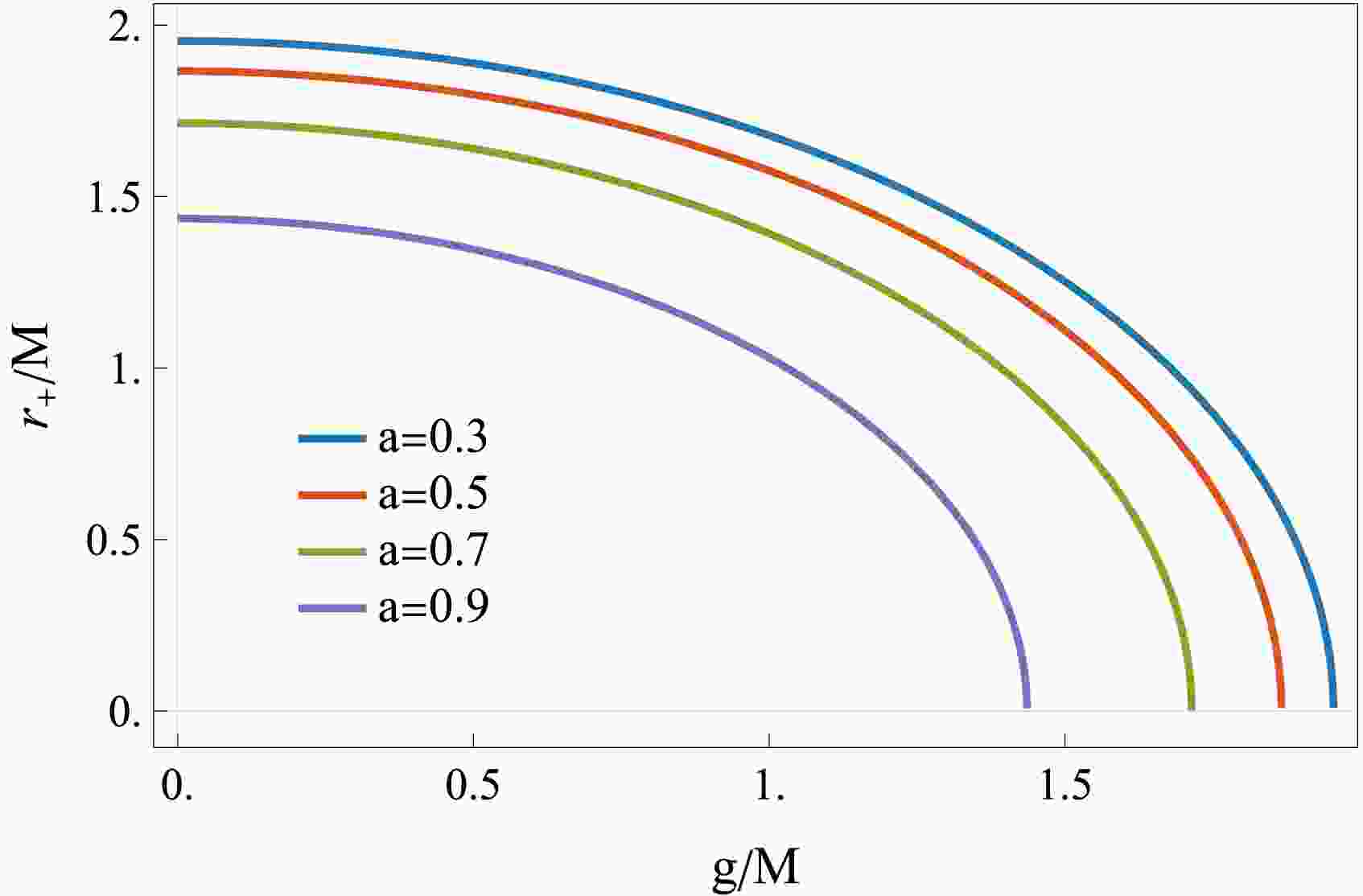
$ 0 \le g \lt M+ \sqrt{M^2-a^2} $ in the subsequent analysis. To illustrate the impact of g on the horizon geometry, Fig. 1 displays the variation of the outer horizon radius$ r_+ $ with g for several representative values of a. As g increases, the outer horizon radius decreases monotonically and may become significantly smaller than its Kerr value, underscoring the strong influence of spacetime regularization on the near-horizon geometry.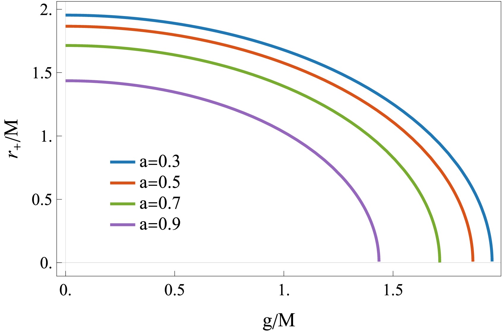
Figure 1. (color online) Variation of the event horizon radius
$ r_+ $ as a function of the parameter g for several representative values of a.The dynamics of test particles in the equatorial plane are of fundamental importance for modeling astrophysical accretion disks [71]. In the standard thin-disk model, the accreting matter is assumed to follow nearly circular, equatorial orbits prior to plunging into the black hole. Therefore, a detailed analysis of equatorial circular orbits is essential for understanding the radiative properties and observational signatures of accretion disks around the rotating SV black hole, as explored below. Restricting the motion to the equatorial plane, we impose the conditions
$ \theta=\pi/2 $ and$ \dot{\theta}=0 $ . The particle's motion is then governed by the Lagrangian$ {\cal{L}} =\frac{1}{2} g_{\mu\nu}\dot{x}^{\mu}\dot{x}^{\nu} =\frac{1}{2}\left( g_{tt}\dot{t}^{2} +2g_{t\phi}\dot{t}\dot{\phi} +g_{rr}\dot{r}^{2} +g_{\phi\phi}\dot{\phi}^{2} \right), $
(4) where an overdot denotes differentiation with respect to the proper time. Owing to the stationarity and axial symmetry of the spacetime, the coordinates t and ϕ are cyclic. The conjugate momenta, derived from the Lagrangian,
$ p_{\mu}=\dfrac{\partial{\cal{L}}}{\partial\dot{x}^{\mu}}, $ lead to two conserved quantities along geodesics: the energy E and the angular momentum L, defined as$ E=-p_{t}=-g_{tt}\dot{t} - g_{t\phi}\dot{\phi}, $
(5) $ L=p_{\phi}=g_{t\phi}\dot{t} + g_{\phi\phi}\dot{\phi}. $
(6) Under the assumption of equatorial circular motion, the dynamics of test particles can be derived by following the standard procedure presented in [71]. We impose the circular-orbit condition
$ \dot{r}=0 $ and express the angular velocity$ \Omega=d\phi/dt=\dot{\phi}/\dot{t} $ in the general form$ \Omega_{\pm} = \frac{-\partial_r g_{t\phi} \pm \sqrt{(\partial_r g_{t\phi})^2 - (\partial_r g_{tt})(\partial_r g_{\phi\phi})}} {\partial_r g_{\phi\phi}}, $
(7) where the plus and minus signs correspond to co-rotating and counter-rotating circular orbits, respectively. Unless otherwise stated, we focus on the co-rotating branch
$ \Omega=\Omega_{+} $ , i.e., particles move counterclockwise for a face-on observer. For a massive test particle, the motion is subject to the normalization condition of the four-velocity$ g_{\mu\nu}x^\mu x^\nu=-1 $ . The conserved energy and angular momentum are then given by$ E = \frac{-g_{tt}-g_{t\phi}\Omega} {\sqrt{-g_{tt}-2g_{t\phi}\Omega-g_{\phi\phi}\Omega^2}}, $
(8) $ L = \frac{g_{t\phi}+g_{\phi\phi}\Omega} {\sqrt{-g_{tt}-2g_{t\phi}\Omega-g_{\phi\phi}\Omega^2}} . $
(9) Having obtained the analytical expressions for the specific energy E, angular momentum L, and angular velocity Ω of test particles on equatorial circular orbits, we now investigate their numerical behavior as functions of the radial coordinate r for different choices of the model parameters. The results are summarized in Fig. 2, which presents four representative parameter sets. The Schwarzschild case corresponds to
$ a=0 $ and$ g=0 $ , whereas the Kerr spacetime is recovered for$ g=0 $ and$ a\neq0 $ ; the remaining curves describe rotating regular SV black holes with nonvanishing g. For each curve, the leftmost endpoint marks the location of the ISCO, which sets the natural inner edge of stable particle motion. Accordingly, all quantities are shown only for radii larger than the corresponding ISCO radius. From Fig. 2, several characteristic trends can be identified. For fixed a, increasing g leads to an increase in the specific energy E and angular momentum L at a given radius, while the angular velocity Ω correspondingly decreases. This indicates that spacetime regularization effectively allows particles to orbit with higher energy and angular momentum, while rotating more slowly. In contrast, for fixed g, increasing a results in a systematic reduction of E, L, and Ω, reflecting the well-known effect of frame dragging in rotating spacetimes. Notably, although the parameter g affects the radial dependence of these quantities, the values of E, L, and Ω evaluated at the ISCO remain unchanged when g varies at fixed a. This demonstrates that, although the location of the ISCO depends on the spacetime regularization parameter g, the corresponding orbital properties of particles at the ISCO are insensitive to g.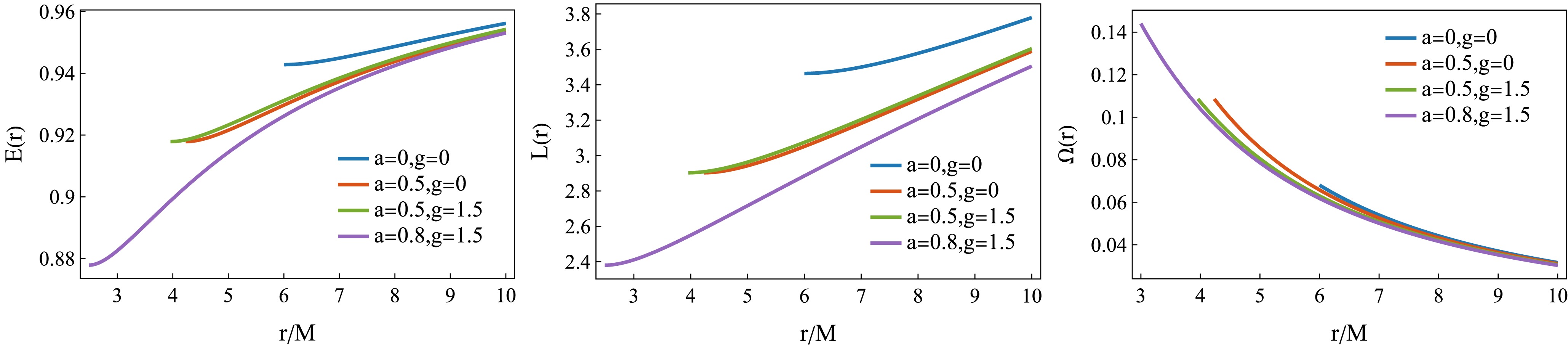
Figure 2. (color online) Radial profiles of the specific energy E, specific angular momentum L, and angular velocity Ω for particles on prograde, equatorial, circular orbits.
For the motion of massive particles confined to the equatorial plane, the radial equation of motion can be written as
$ \begin{aligned}[b] & g_{rr}\dot r^{2}+V_{{\rm{eff}}}(r)=0,\\ & V_{{\rm{eff}}}(r)\equiv 1-\frac{E^{2}g_{\phi\phi}+2ELg_{t\phi}+L^{2}g_{tt}}{g_{t\phi}^{2}-g_{tt}g_{\phi\phi}}, \end{aligned} $
(10) where
$ V_{{\rm{eff}}}(r) $ denotes the radial effective potential. The location of the ISCO is determined by the following equation$ \frac{d^{2}V_{{\rm{eff}}}}{dr^{2}}=0. $
(11) Since this condition generally does not admit a closed-form solution, the ISCO radius must be computed numerically.
Figure 3 shows the ISCO radius as a function of the parameters a and g for both prograde and retrograde circular orbits. For prograde motion, the ISCO radius decreases monotonically with increasing a and g. In contrast, for retrograde motion, the ISCO radius increases with increasing a while still decreasing with increasing g. Moreover, in both the prograde and retrograde cases, the ISCO radius depends much more strongly on a than on g, indicating that spacetime rotation plays the dominant role in determining the ISCO location.
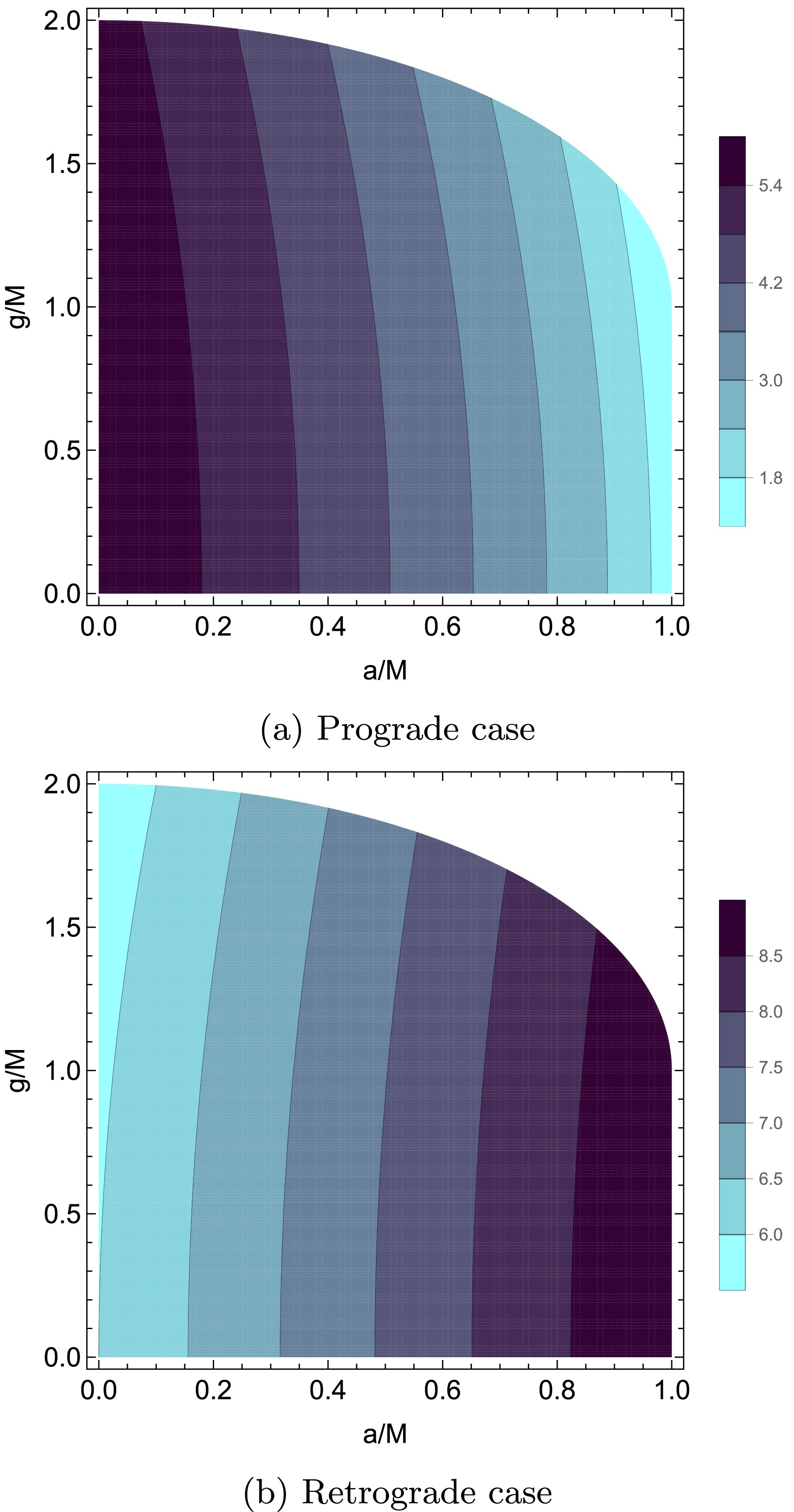
Figure 3. (color online) The ISCO radius as a function of the model parameters a and g.
The radiative efficiency is a key quantity that measures the conversion of gravitational energy into radiation during accretion and is widely used to characterize the energy output of black hole accretion disks [72−79]. Within the thin-disk approximation, assuming that particles slowly inspiral from infinity and terminate their motion at the ISCO, the radiative efficiency is defined as
$ \eta=\frac{E_{\infty}-E_{{\rm{ISCO}}}}{E_{\infty}}, $
(12) where
$ E_{\infty} $ denotes the specific energy of a particle at infinity. For particles starting from rest at infinity, one may approximate$ E_{\infty}\simeq 1 $ , leading to$ \eta \simeq 1 - E_{{\rm{ISCO}}}. $
(13) Figure 4 shows how the radiative efficiency depends on the parameters a and g. As a increases, the radiative efficiency increases markedly, consistent with the well-known behavior in Kerr spacetime. By contrast, varying g does not affect the radiative efficiency. This directly follows from the specific energy evaluated at the ISCO being independent of g. This insensitivity is a typical feature of the SV black hole: spacetime regularization does not modify the efficiency of energy release.
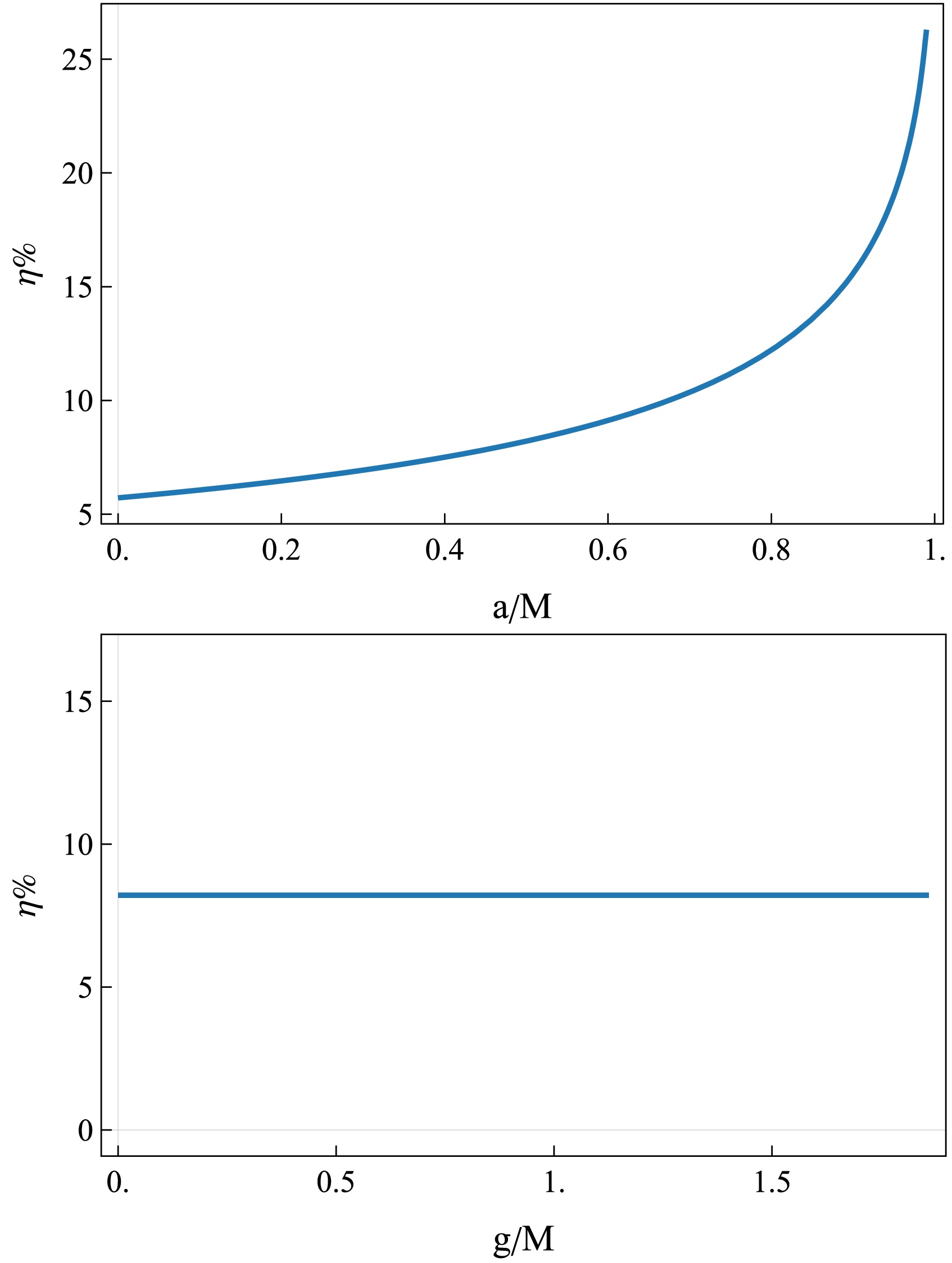
Figure 4. (color online) Radiative efficiency of a rotating SV black hole. The top panel shows the dependence on the spin parameter a for fixed
$ g=1.5 $ , while the bottom panel shows the dependence on g for fixed$ a=0.5 $ . -
The spherically symmetric SV black hole was originally proposed as a regular black hole mimicker by introducing a regularization parameter that removes the central curvature singularity while preserving asymptotic flatness [29, 30]. Using a modified Newman–Janis algorithm, the static SV spacetime can be generalized to a stationary, axisymmetric rotating geometry, referred to as the rotating SV black hole [32, 43]. Working in natural units with
$ G=c=1 $ , the line element of the rotating SV black hole in Boyer–Lindquist coordinates$ (t,r,\theta,\phi) $ is given by$ \begin{aligned}[b] {\rm d}s^{2} ={}& -\left(1-\frac{2 M \sqrt{r^{2}+g^{2}}}{\rho^2}\right) {\rm d}t^{2} + \frac{\rho^2}{\Delta} \, {\rm d}r^{2} + \rho^2 \, {\rm d}\theta^{2} \\ &- \frac{4 a M \sqrt{r^{2}+g^{2}} \sin^{2}\theta}{\rho^2} \, {\rm d}t \, {\rm d}\phi + \frac{\Sigma \sin^2\theta}{\rho^2} \, {\rm d}\phi^{2}, \end{aligned} $
(1) where
$ \begin{aligned}[b] &\rho^2 = r^2 + g^2 + a^2\cos^2\theta, \quad \Delta = r^2 + g^2 + a^2 - 2M\sqrt{r^2 + g^2}, \\ &\Sigma = (r^2 + g^2 + a^2)^2 - \Delta a^2 \sin^2\theta. \\[-13pt]\end{aligned} $
(2) Here, M denotes the ADM mass; a is the spin parameter associated with the black hole's angular momentum; and g is a regularization parameter that characterizes deviations from the Kerr geometry and ensures spacetime regularity. In the limit
$ g\to0 $ , the metric reduces to the Kerr solution, while for$ a\to0 $ , it further reduces to the Schwarzschild solution.The condition
$ \Delta(r)=0 $ defines the event horizons of the rotating regular spacetime. This equation admits analytic solutions, yielding two positive roots that correspond to the inner and outer horizons,$ r_- $ and$ r_+ $ , respectively.$ r_{\pm} = \sqrt{(M \pm \sqrt{M^2-a^2})^2 - g^2}. $
(3) The existence and number of horizons are jointly controlled by the parameters a and g. Depending on the value of g, the rotating SV spacetime falls into three distinct regimes, as summarized in Table 1. A comprehensive discussion of the global parameter space is provided in [32].
Range of g Horizons Spacetime $ [0,M-\sqrt{M^2-a^2}) $ $ r_-,\,r_+ $ Regular black hole $ [M-\sqrt{M^2-a^2} , M+\sqrt{M^2-a^2}) $ $ r_+ $ Single-horizon regular
black hole$ [M+\sqrt{M^2-a^2},\infty) $ No horizon Wormhole Table 1. Classification of rotating SV spacetimes according to the parameter g [32].
In this work, we focus exclusively on regular black hole configurations that possess an outer event horizon. Accordingly, we restrict g to the range
$ 0 \le g \lt M+ \sqrt{M^2-a^2} $ in the subsequent analysis. To illustrate the impact of g on the horizon geometry, Fig. 1 displays the variation of the outer horizon radius$ r_+ $ with g for several representative values of a. As g increases, the outer horizon radius decreases monotonically and may become significantly smaller than its Kerr value, underscoring the strong influence of spacetime regularization on the near-horizon geometry.
Figure 1. (color online) Variation of the event horizon radius
$ r_+ $ as a function of the parameter g for several representative values of a.The dynamics of test particles in the equatorial plane are of fundamental importance for modeling astrophysical accretion disks [71]. In the standard thin-disk model, the accreting matter is assumed to follow nearly circular, equatorial orbits prior to plunging into the black hole. Therefore, a detailed analysis of equatorial circular orbits is essential for understanding the radiative properties and observational signatures of accretion disks around the rotating SV black hole, as explored below. Restricting the motion to the equatorial plane, we impose the conditions
$ \theta=\pi/2 $ and$ \dot{\theta}=0 $ . The particle's motion is then governed by the Lagrangian$ {\cal{L}} =\frac{1}{2} g_{\mu\nu}\dot{x}^{\mu}\dot{x}^{\nu} =\frac{1}{2}\left( g_{tt}\dot{t}^{2} +2g_{t\phi}\dot{t}\dot{\phi} +g_{rr}\dot{r}^{2} +g_{\phi\phi}\dot{\phi}^{2} \right), $
(4) where an overdot denotes differentiation with respect to the proper time. Owing to the stationarity and axial symmetry of the spacetime, the coordinates t and ϕ are cyclic. The conjugate momenta, derived from the Lagrangian,
$ p_{\mu}=\dfrac{\partial{\cal{L}}}{\partial\dot{x}^{\mu}}, $ lead to two conserved quantities along geodesics: the energy E and the angular momentum L, defined as$ E=-p_{t}=-g_{tt}\dot{t} - g_{t\phi}\dot{\phi}, $
(5) $ L=p_{\phi}=g_{t\phi}\dot{t} + g_{\phi\phi}\dot{\phi}. $
(6) Under the assumption of equatorial circular motion, the dynamics of test particles can be derived by following the standard procedure presented in [71]. We impose the circular-orbit condition
$ \dot{r}=0 $ and express the angular velocity$ \Omega={\rm d}\phi/{\rm d}t=\dot{\phi}/\dot{t} $ in the general form$ \Omega_{\pm} = \frac{-\partial_r g_{t\phi} \pm \sqrt{(\partial_r g_{t\phi})^2 - (\partial_r g_{tt})(\partial_r g_{\phi\phi})}} {\partial_r g_{\phi\phi}}, $
(7) where the plus and minus signs correspond to co-rotating and counter-rotating circular orbits, respectively. Unless otherwise stated, we focus on the co-rotating branch
$ \Omega=\Omega_{+} $ , i.e., particles move counterclockwise for a face-on observer. For a massive test particle, the motion is subject to the normalization condition of the four-velocity$ g_{\mu\nu}x^\mu x^\nu=-1 $ . The conserved energy and angular momentum are then given by$ E = \frac{-g_{tt}-g_{t\phi}\Omega} {\sqrt{-g_{tt}-2g_{t\phi}\Omega-g_{\phi\phi}\Omega^2}}, $
(8) $ L = \frac{g_{t\phi}+g_{\phi\phi}\Omega} {\sqrt{-g_{tt}-2g_{t\phi}\Omega-g_{\phi\phi}\Omega^2}} . $
(9) Having obtained the analytical expressions for the specific energy E, angular momentum L, and angular velocity Ω of test particles on equatorial circular orbits, we now investigate their numerical behavior as functions of the radial coordinate r for different choices of the model parameters. The results are summarized in Fig. 2, which presents four representative parameter sets. The Schwarzschild case corresponds to
$ a=0 $ and$ g=0 $ , whereas the Kerr spacetime is recovered for$ g=0 $ and$ a\neq0 $ ; the remaining curves describe rotating regular SV black holes with nonvanishing g. For each curve, the leftmost endpoint marks the location of the ISCO, which sets the natural inner edge of stable particle motion. Accordingly, all quantities are shown only for radii larger than the corresponding ISCO radius. From Fig. 2, several characteristic trends can be identified. For fixed a, increasing g leads to an increase in the specific energy E and angular momentum L at a given radius, while the angular velocity Ω correspondingly decreases. This indicates that spacetime regularization effectively allows particles to orbit with higher energy and angular momentum, while rotating more slowly. In contrast, for fixed g, increasing a results in a systematic reduction of E, L, and Ω, reflecting the well-known effect of frame dragging in rotating spacetimes. Notably, although the parameter g affects the radial dependence of these quantities, the values of E, L, and Ω evaluated at the ISCO remain unchanged when g varies at fixed a. This demonstrates that, although the location of the ISCO depends on the spacetime regularization parameter g, the corresponding orbital properties of particles at the ISCO are insensitive to g.
Figure 2. (color online) Radial profiles of the specific energy E, specific angular momentum L, and angular velocity Ω for particles on prograde, equatorial, circular orbits.
For the motion of massive particles confined to the equatorial plane, the radial equation of motion can be written as
$ \begin{aligned}[b] & g_{rr}\dot r^{2}+V_{{\rm{eff}}}(r)=0,\\ & V_{{\rm{eff}}}(r)\equiv 1-\frac{E^{2}g_{\phi\phi}+2ELg_{t\phi}+L^{2}g_{tt}}{g_{t\phi}^{2}-g_{tt}g_{\phi\phi}}, \end{aligned} $
(10) where
$ V_{{\rm{eff}}}(r) $ denotes the radial effective potential. The location of the ISCO is determined by the following equation$ \frac{{\rm d}^{2}V_{{\rm{eff}}}}{{\rm d}r^{2}}=0. $
(11) Since this condition generally does not admit a closed-form solution, the ISCO radius must be computed numerically.
Figure 3 shows the ISCO radius as a function of the parameters a and g for both prograde and retrograde circular orbits. For prograde motion, the ISCO radius decreases monotonically with increasing a and g. In contrast, for retrograde motion, the ISCO radius increases with increasing a while still decreasing with increasing g. Moreover, in both the prograde and retrograde cases, the ISCO radius depends much more strongly on a than on g, indicating that spacetime rotation plays the dominant role in determining the ISCO location.
Figure 3. (color online) The ISCO radius as a function of the model parameters a and g.
The radiative efficiency is a key quantity that measures the conversion of gravitational energy into radiation during accretion and is widely used to characterize the energy output of black hole accretion disks [72−79]. Within the thin-disk approximation, assuming that particles slowly inspiral from infinity and terminate their motion at the ISCO, the radiative efficiency is defined as
$ \eta=\frac{E_{\infty}-E_{{\rm{ISCO}}}}{E_{\infty}}, $
(12) where
$ E_{\infty} $ denotes the specific energy of a particle at infinity. For particles starting from rest at infinity, one may approximate$ E_{\infty}\simeq 1 $ , leading to$ \eta \simeq 1 - E_{{\rm{ISCO}}}. $
(13) Figure 4 shows how the radiative efficiency depends on the parameters a and g. As a increases, the radiative efficiency increases markedly, consistent with the well-known behavior in Kerr spacetime. By contrast, varying g does not affect the radiative efficiency. This directly follows from the specific energy evaluated at the ISCO being independent of g. This insensitivity is a typical feature of the SV black hole: spacetime regularization does not modify the efficiency of energy release.
Figure 4. (color online) Radiative efficiency of a rotating SV black hole. The top panel shows the dependence on the spin parameter a for fixed
$ g=1.5 $ , while the bottom panel shows the dependence on g for fixed$ a=0.5 $ . -
In the previous section, we analyzed the dynamical properties of equatorial circular orbits and the structure of the ISCO in the rotating SV black hole spacetime. Building on these results, we now investigate the radiative properties of thin accretion disks in this background, with particular emphasis on the radial distribution of the radiative flux. Within the Novikov–Thorne thin-disk model, the radiative flux emitted by the disk surface is given by [72, 80−82]:
$ {\cal{F}}(r)=\frac{\dot{M}}{4\pi\sqrt{-\tilde{g}/g_{\theta\theta}}} \frac{-\Omega_{,r}}{(E-\Omega L)^2} \int_{r_{{\rm{ISCO}}}}^{r}(E-\Omega L)L_{,r}\,dr, $
(14) where
$ \dot{M} $ is the mass accretion rate, assumed to be constant here, and$ \tilde{g} $ denotes the determinant of the spacetime metric.Once the radiative flux from the accretion disk surface is obtained, one can then define the local effective temperature of the disk. Assuming that the disk emits locally as a blackbody, the radiative flux and the effective temperature are related through the Stefan–Boltzmann law [83]. Accordingly, the local effective temperature of the accretion disk at radius r is given by
$ T_{{\rm{eff}}}(r) =\left(\frac{{\cal{F}}(r)}{\sigma}\right)^{1/4}, $
(15) where σ denotes the Stefan–Boltzmann constant, whose numerical value is
$ \sigma = 5.67 \times 10^{-5}\; {\rm{erg}}\,{\rm{cm}}^{-2}\,{\rm{s}}^{-1}\,{\rm{K}}^{-4}. $
(16) To remove the overall scaling effects induced by the black-hole mass and the mass-accretion rate, we introduce dimensionless forms of the radiative flux and the effective temperature [84]. Specifically, the dimensionless radiative flux,
$ {\cal{F}}^* $ , and the dimensionless effective temperature,$ T_{{\rm{eff}}}^* $ , are defined as$ {\cal{F}}^*=\frac{G^2 M^2}{c^6 \dot{M}}\,{\cal{F}}, \qquad T_{{\rm{eff}}}^* = {\cal{F}}^{*1/4}, $
(17) where G is the gravitational constant, c is the speed of light in vacuum, and M and
$ \dot{M} $ denote the black hole mass and mass accretion rate, respectively. With these dimensionless quantities, the radiative flux and effective temperature distributions of accretion disks around black holes with different masses and accretion rates can be directly compared. The corresponding numerical results are presented and discussed in the following figures.Figure 5 presents numerical results for the dimensionless radiative flux
$ {\cal{F}}^* $ in two representative scenarios: varying g at fixed a, and varying a at fixed g. In all cases, the radial profiles of the radiative flux exhibit a well-defined peak whose magnitude and radial location depend sensitively on these parameters. The upper panel shows four representative curves obtained for fixed$ g=1 $ and different values of a. As a increases, the radiative flux is enhanced at all radii, the peak value increases significantly, and the peak shifts inward. This indicates that the spin parameter plays a dominant role in shaping the disk’s radiative properties. In particular, the maximum radiative flux for$ a=0.8 $ is approximately three times that for$ a=0.5 $ , highlighting the strong impact of black hole spin.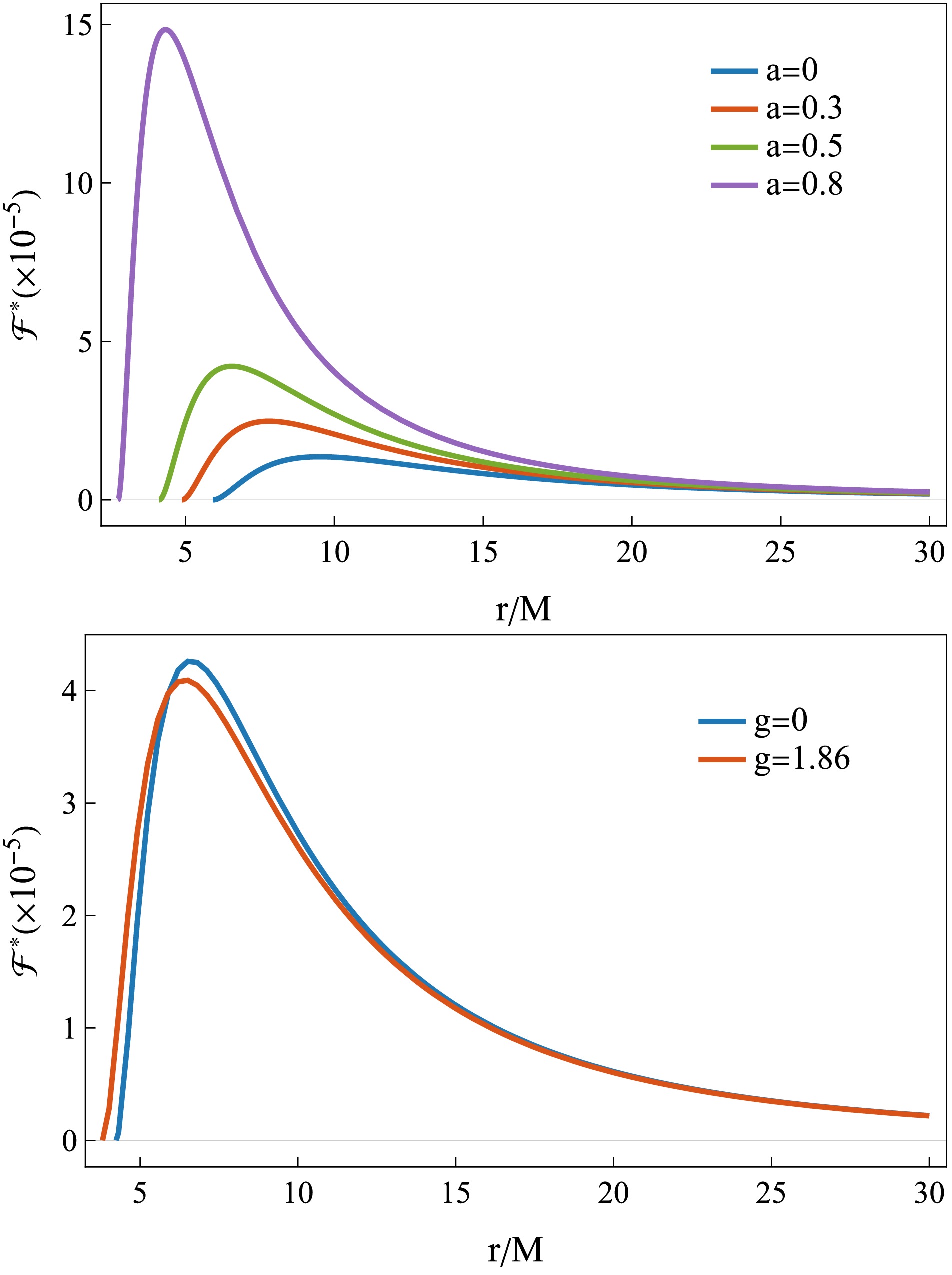
Figure 5. (color online) Dimensionless radiative flux from a thin accretion disk around a rotating SV black hole. The top panel shows the flux as a function of a for fixed
$ g=1 $ . The bottom panel shows the flux as a function of g for fixed$ a=0.5 $ .The lower panel corresponds to the case with fixed
$ a=0.5 $ , with g taking values$ g=0 $ and$ g=1.86 $ , the latter being close to the upper bound permitted for regular black hole configurations. This choice maximizes the visibility of the effects induced by g. It is evident that, within the parameter range allowed by regular black hole solutions, the influence of g on the radiative flux is much weaker than that of a. As g increases, the peak radiative flux decreases and the peak shifts slightly inward. However, this trend is not monotonic across the disk: in some regions, the radiative flux is instead slightly enhanced.We next present the numerical results for the dimensionless effective temperature in Fig. 6, with model parameters identical to those used in the previous analysis of the dimensionless radiative flux. We find that the influence of parameters a and g on the effective temperature follows the same qualitative trend as for the radiative flux, although the overall variation is much weaker. This behavior arises because the effective temperature scales with the radiative flux as
$ T_{{\rm{eff}}} \propto {\cal{F}}^{1/4} $ , which significantly suppresses the impact of parameter variations. We now restore physical units and examine whether observationally distinguishable features from the Kerr case can arise in the rotating SV black hole. Therefore, we consider two representative astrophysical examples: the supermassive black holes Sgr A* and M87*. In our numerical calculations, we adopt the following physical constants: the speed of light$ c = 3\times10^{10}\,{\rm{cm}}\,{\rm{s}}^{-1} $ , the Planck constant$ h = 6.625\times10^{-27}\,{\rm{erg}}\,{\rm{s}} $ , the Boltzmann constant$ k = 1.38\times10^{-16}\,{\rm{erg}}\,K^{-1} $ , the solar mass$ M_\odot = 1.989\times10^{33}\,{\rm{g}} $ , and$ 1\; {\rm{year}} = 3.156\times10^{7}\,{\rm{s}} $ .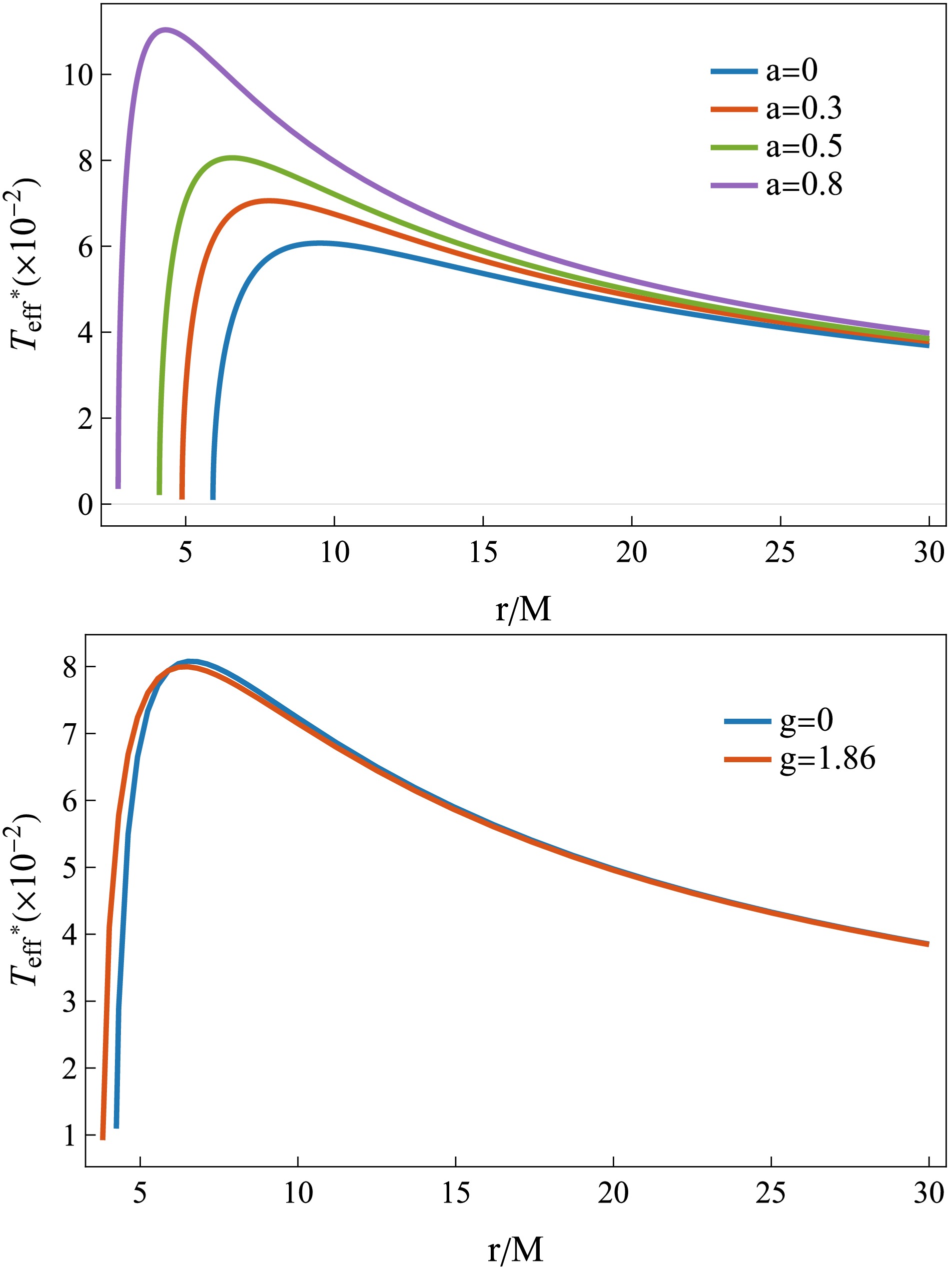
Figure 6. (color online) The dimensionless effective temperature of a thin accretion disk around a rotating SV black hole. The top panel shows its dependence on the spin parameter a for fixed
$ g=1 $ . The bottom panel shows its dependence on the parameter g for fixed$ a=0.5 $ .For Sgr A* [3, 85], the black hole mass and mass accretion rate are taken to be
$ M = 4\times10^{6}\,{\rm{M}}_\odot $ and$ \dot{M}=10^{-6}\,{\rm{M}}_\odot/{\rm{year}} $ , respectively. We focus on the peak values of the radiative flux and the effective temperature. For the rotating SV black hole with$ a=0.5 $ and$ g=1.86 $ , the maximum radiative flux, the maximum effective temperature, and the corresponding radial position are given by$ \begin{aligned}[b] {\cal{F}}_{\max} &= 6.67 \times 10^{12}\ {\rm{erg}}\,{\rm{cm}}^{-2}\,{\rm{s}}^{-1},\\ T_{{\rm{eff}}}^{\max} &= 1.85 \times 10^{4}\ {\rm{K}},\\ r_{\max} &= 6.42\, M . \end{aligned} $
(18) For comparison, the corresponding quantities for a Kerr black hole with the same spin parameter,
$ a=0.5 $ , are given by$ \begin{aligned}[b] {\cal{F}}_{\max} &= 6.95 \times 10^{12}\ {\rm{erg}}\,{\rm{cm}}^{-2}\,{\rm{s}}^{-1},\\ T_{{\rm{eff}}}^{\max} &= 1.87 \times 10^{4}\ {\rm{K}},\\ r_{\max} &= 6.62\, M . \end{aligned} $
(19) As a second example, we consider M87* [2], whose black hole mass and mass accretion rate are taken to be
$ M = 6.5\times10^{9}\,{\rm{M}}_\odot $ and$ \dot{M}=10^{-3}\,{\rm{M}}_\odot/{\rm{year}} $ [86]. For a rotating SV black hole with$ a=0.8 $ [86] and$ g=1.5 $ , we obtain$ \begin{aligned}[b] {\cal{F}}_{\max} &= 8.85 \times 10^{9}\ {\rm{erg}}\,{\rm{cm}}^{-2}\,{\rm{s}}^{-1},\\ T_{{\rm{eff}}}^{\max} &= 3.53 \times 10^{3}\ {\rm{K}},\\ r_{\max} &= 4.22\, M . \end{aligned} $
(20) For the Kerr black hole with
$ a=0.8 $ , the corresponding results are as follows.$ \begin{aligned}[b] {\cal{F}}_{\max} &= 9.40 \times 10^{9}\ {\rm{erg}}\,{\rm{cm}}^{-2}\,{\rm{s}}^{-1},\\ T_{{\rm{eff}}}^{\max} &= 3.59 \times 10^{3}\ {\rm{K}},\\ r_{\max} &= 4.42\, M . \end{aligned} $
(21) It should be emphasized that the radiative flux and the effective temperature are defined in the local rest frame of the accretion disk and, therefore, are not directly observable quantities. From an observational perspective, a more relevant quantity is the spectral luminosity
$ \nu {\cal{L}}_{\nu,\infty} $ , as measured by a distant observer, which encodes the global radiative properties of the disk [79, 87, 88]. Assuming the disk emits as a collection of local blackbody radiators and neglecting light bending, the spectral luminosity at infinity is obtained by integrating the local emission over the entire disk surface. Under the thin-disk approximation, the spectral luminosity takes the form$ \nu {\cal{L}}_{\nu,\infty} = \frac{8\pi h \cos\gamma}{c^{2}} \int_{r_{{\rm{ISCO}}}}^{r_{{\rm{out}}}} \int_{0}^{2\pi} \frac{\nu \nu_{e}^{3} r\,dr\,d\phi} {\exp \left(\dfrac{h\nu_{e}}{k\, T_{{\rm{eff}}}(r)}\right)-1}, $
(22) where
$ r_{{\rm{out}}} $ denotes the outer edge of the accretion disk and is chosen sufficiently large to ensure convergence of the numerical integration. The parameter γ represents the inclination angle of the accretion disk. For the equatorial accretion disk considered here,$ \gamma=0 $ . The symbols ν and$ \nu_e $ denote, respectively, the observed frequency at infinity and the emitted frequency measured in the local rest frame of the accretion disk; they are related by$ \nu_e = \nu / g_{{\rm{out}}} $ . The redshift factor$ g_{{\rm{out}}} $ is determined by the spacetime geometry and the orbital motion of the disk matter and is given by$ g_{{\rm{out}}} = \sqrt{- g_{tt}- 2 g_{t\phi}\Omega- g_{\phi\phi}\Omega^{2}}. $
(23) The next section presents a detailed analysis of the redshift factor and its role in shaping the observed radiation.
For the numerical evaluation of the spectral luminosity, we fix the outer edge of the accretion disk at
$ r_{{\rm{out}}}=1000M $ and set the inclination angle to$ \gamma=0 $ , while the black hole mass and the mass accretion rate are chosen to be consistent with observational estimates for Sgr A*. Under these assumptions, the spectral luminosity$ \nu{\cal{L}}_{\nu,\infty} $ of rotating regular black holes in the frequency range$ 10^{13} $ –$ 10^{16}{\rm{Hz}} $ is computed for different values of the spin parameter a and the regularization parameter g, as shown in Fig. 7. In this frequency band, the spectral luminosity always exhibits a pronounced maximum, which serves as the main quantity of interest in the following discussion. In the upper panel, for fixed$ g=1 $ , the spectral luminosity increases significantly with increasing spin. In particular, for$ a=0 $ , corresponding to the spherically symmetric SV black hole, the maximum value is$ \nu{\cal{L}}_{\nu,\infty}^{{\rm{max}}}=3.049\times10^{39}{\rm{erg}}\,{\rm{s}}^{-1} $ , occurring at$ \nu=6.40\times10^{14}{\rm{Hz}} $ , whereas for$ a=0.8 $ the peak rises to$ \nu{\cal{L}}_{\nu,\infty}^{{\rm{max}}}=6.339\times 10^{39}{\rm{erg}}\,{\rm{s}}^{-1} $ , occurring at$ \nu=1.02\times10^{15}{\rm{Hz}} $ , i.e., more than twice the maximum value for the$ a=0 $ case. In contrast, the lower panel shows that for a rotating SV black hole with fixed spin$ a=0.5 $ , the dependence on the parameter g is much weaker: when g varies from$ 0 $ to$ 1.86 $ , the peak value decreases slightly from$ 4.350\times10^{39}{\rm{erg}}\,{\rm{s}}^{-1} $ at$ \nu=8.10\times10^{14}{\rm{Hz}} $ to$ 4.311\times10^{39}{\rm{erg}}\,{\rm{s}}^{-1} $ at$ \nu=8.03\times 10^{14}{\rm{Hz}} $ . Both the peak amplitude and its corresponding frequency are therefore marginally smaller for larger g, and the Kerr case ($ g=0 $ ) yields a maximum spectral luminosity approximately$ 1.01 $ times that of the rotating SV black hole at$ g=1.86 $ .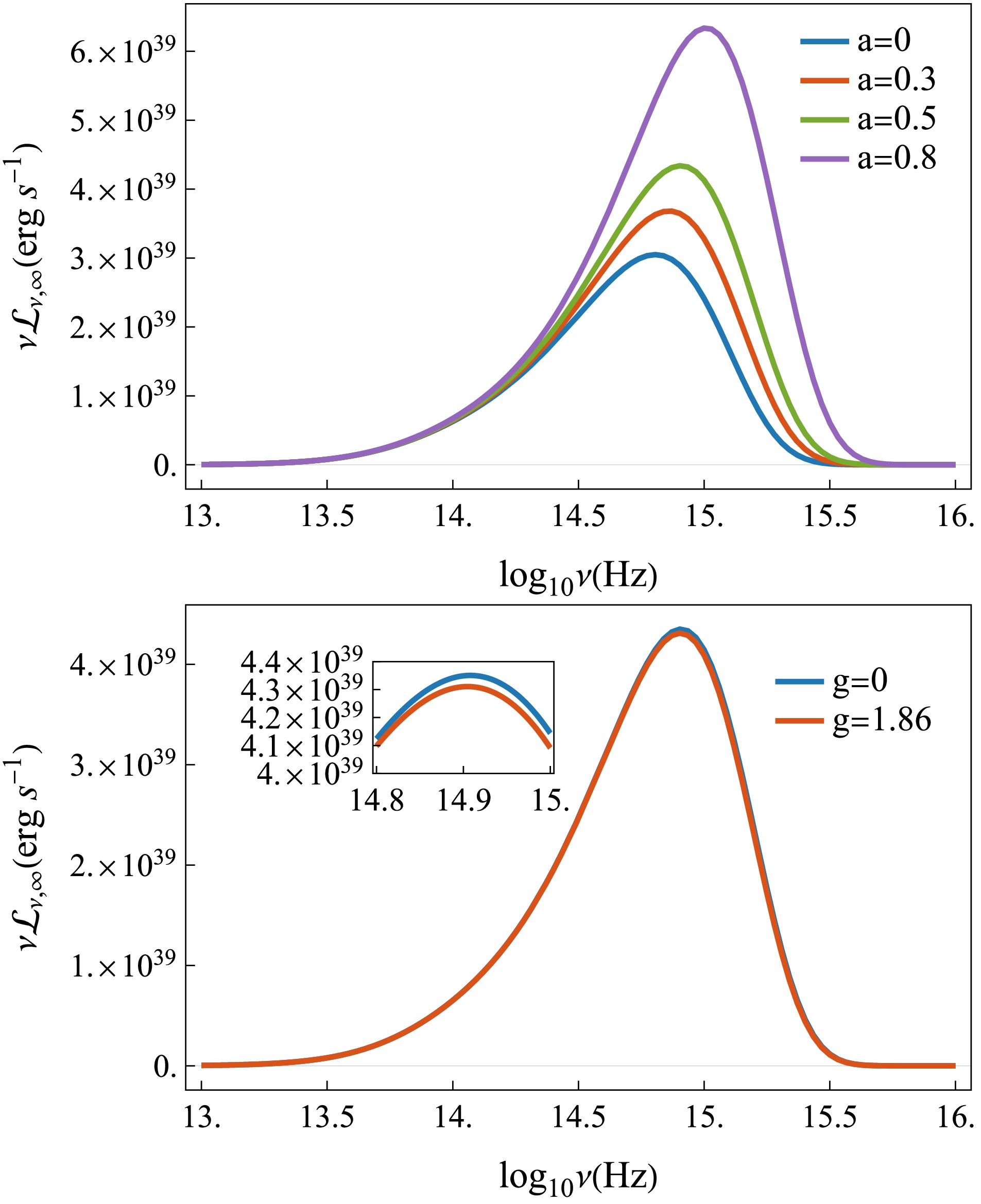
Figure 7. (color online) Spectral luminosity of a thin accretion disk around a rotating SV black hole. The top panel shows the dependence on the parameter a for fixed
$ g=1 $ . The bottom panel shows the dependence on the parameter g for fixed$ a=0.5 $ . -
In the previous section, we analyzed the dynamical properties of equatorial circular orbits and the structure of the ISCO in the rotating SV black hole spacetime. Building on these results, we now investigate the radiative properties of thin accretion disks in this background, with particular emphasis on the radial distribution of the radiative flux. Within the Novikov–Thorne thin-disk model, the radiative flux emitted by the disk surface is given by [72, 80−82]:
$ {\cal{F}}(r)=\frac{\dot{M}}{4\pi\sqrt{-\tilde{g}/g_{\theta\theta}}} \frac{-\Omega_{,r}}{(E-\Omega L)^2} \int_{r_{{\rm{ISCO}}}}^{r}(E-\Omega L)L_{,r}\,{\rm d}r, $
(14) where
$ \dot{M} $ is the mass accretion rate, assumed to be constant here, and$ \tilde{g} $ denotes the determinant of the spacetime metric.Once the radiative flux from the accretion disk surface is obtained, one can then define the local effective temperature of the disk. Assuming that the disk emits locally as a blackbody, the radiative flux and the effective temperature are related through the Stefan–Boltzmann law [83]. Accordingly, the local effective temperature of the accretion disk at radius r is given by
$ T_{{\rm{eff}}}(r) =\left(\frac{{\cal{F}}(r)}{\sigma}\right)^{1/4}, $
(15) where σ denotes the Stefan–Boltzmann constant, whose numerical value is
$ \sigma = 5.67 \times 10^{-5}\; {\rm{erg}}\,{\rm{cm}}^{-2}\,{\rm{s}}^{-1}\,{\rm{K}}^{-4}. $
(16) To remove the overall scaling effects induced by the black-hole mass and the mass-accretion rate, we introduce dimensionless forms of the radiative flux and the effective temperature [84]. Specifically, the dimensionless radiative flux,
$ {\cal{F}}^* $ , and the dimensionless effective temperature,$ T_{{\rm{eff}}}^* $ , are defined as$ {\cal{F}}^*=\frac{G^2 M^2}{c^6 \dot{M}}\,{\cal{F}}, \qquad T_{{\rm{eff}}}^* = {\cal{F}}^{*1/4}, $
(17) where G is the gravitational constant, c is the speed of light in vacuum, and M and
$ \dot{M} $ denote the black hole mass and mass accretion rate, respectively. With these dimensionless quantities, the radiative flux and effective temperature distributions of accretion disks around black holes with different masses and accretion rates can be directly compared. The corresponding numerical results are presented and discussed in the following figures.Figure 5 presents numerical results for the dimensionless radiative flux
$ {\cal{F}}^* $ in two representative scenarios: varying g at fixed a, and varying a at fixed g. In all cases, the radial profiles of the radiative flux exhibit a well-defined peak whose magnitude and radial location depend sensitively on these parameters. The upper panel shows four representative curves obtained for fixed$ g=1 $ and different values of a. As a increases, the radiative flux is enhanced at all radii, the peak value increases significantly, and the peak shifts inward. This indicates that the spin parameter plays a dominant role in shaping the disk’s radiative properties. In particular, the maximum radiative flux for$ a=0.8 $ is approximately three times that for$ a=0.5 $ , highlighting the strong impact of black hole spin.
Figure 5. (color online) Dimensionless radiative flux from a thin accretion disk around a rotating SV black hole. The top panel shows the flux as a function of a for fixed
$ g=1 $ . The bottom panel shows the flux as a function of g for fixed$ a=0.5 $ .The lower panel corresponds to the case with fixed
$ a=0.5 $ , with g taking values$ g=0 $ and$ g=1.86 $ , the latter being close to the upper bound permitted for regular black hole configurations. This choice maximizes the visibility of the effects induced by g. It is evident that, within the parameter range allowed by regular black hole solutions, the influence of g on the radiative flux is much weaker than that of a. As g increases, the peak radiative flux decreases and the peak shifts slightly inward. However, this trend is not monotonic across the disk: in some regions, the radiative flux is instead slightly enhanced.We next present the numerical results for the dimensionless effective temperature in Fig. 6, with model parameters identical to those used in the previous analysis of the dimensionless radiative flux. We find that the influence of parameters a and g on the effective temperature follows the same qualitative trend as for the radiative flux, although the overall variation is much weaker. This behavior arises because the effective temperature scales with the radiative flux as
$ T_{{\rm{eff}}} \propto {\cal{F}}^{1/4} $ , which significantly suppresses the impact of parameter variations. We now restore physical units and examine whether observationally distinguishable features from the Kerr case can arise in the rotating SV black hole. Therefore, we consider two representative astrophysical examples: the supermassive black holes Sgr A* and M87*. In our numerical calculations, we adopt the following physical constants: the speed of light$ c = 3\times10^{10}\,{\rm{cm}}\,{\rm{s}}^{-1} $ , the Planck constant$ h = 6.625\times10^{-27}\,{\rm{erg}}\,{\rm{s}} $ , the Boltzmann constant$ k = 1.38\times 10^{-16}\,{\rm{erg}}\,K^{-1} $ , the solar mass$ M_\odot = 1.989\times10^{33}\,{\rm{g}} $ , and$ 1\; {\rm{year}} = 3.156\times10^{7}\,{\rm{s}} $ .
Figure 6. (color online) The dimensionless effective temperature of a thin accretion disk around a rotating SV black hole. The top panel shows its dependence on the spin parameter a for fixed
$ g=1 $ . The bottom panel shows its dependence on the parameter g for fixed$ a=0.5 $ .For Sgr A* [3, 85], the black hole mass and mass accretion rate are taken to be
$ M = 4\times10^{6}\,{\rm{M}}_\odot $ and$ \dot{M}= 10^{-6}\,{\rm{M}}_\odot/{\rm{year}} $ , respectively. We focus on the peak values of the radiative flux and the effective temperature. For the rotating SV black hole with$ a=0.5 $ and$ g=1.86 $ , the maximum radiative flux, the maximum effective temperature, and the corresponding radial position are given by$ \begin{aligned}[b] {\cal{F}}_{\max} &= 6.67 \times 10^{12}\ {\rm{erg}}\,{\rm{cm}}^{-2}\,{\rm{s}}^{-1},\\ T_{{\rm{eff}}}^{\max} &= 1.85 \times 10^{4}\ {\rm{K}},\\ r_{\max} &= 6.42\, M . \end{aligned} $
(18) For comparison, the corresponding quantities for a Kerr black hole with the same spin parameter,
$ a=0.5 $ , are given by$ \begin{aligned}[b] {\cal{F}}_{\max} &= 6.95 \times 10^{12}\ {\rm{erg}}\,{\rm{cm}}^{-2}\,{\rm{s}}^{-1},\\ T_{{\rm{eff}}}^{\max} &= 1.87 \times 10^{4}\ {\rm{K}},\\ r_{\max} &= 6.62\, M . \end{aligned} $
(19) As a second example, we consider M87* [2], whose black hole mass and mass accretion rate are taken to be
$ M = 6.5\times10^{9}\,{\rm{M}}_\odot $ and$ \dot{M}=10^{-3}\,{\rm{M}}_\odot/{\rm{year}} $ [86]. For a rotating SV black hole with$ a=0.8 $ [86] and$ g=1.5 $ , we obtain$ \begin{aligned}[b] {\cal{F}}_{\max} &= 8.85 \times 10^{9}\ {\rm{erg}}\,{\rm{cm}}^{-2}\,{\rm{s}}^{-1},\\ T_{{\rm{eff}}}^{\max} &= 3.53 \times 10^{3}\ {\rm{K}},\\ r_{\max} &= 4.22\, M . \end{aligned} $
(20) For the Kerr black hole with
$ a=0.8 $ , the corresponding results are as follows.$ \begin{aligned}[b] {\cal{F}}_{\max} &= 9.40 \times 10^{9}\ {\rm{erg}}\,{\rm{cm}}^{-2}\,{\rm{s}}^{-1},\\ T_{{\rm{eff}}}^{\max} &= 3.59 \times 10^{3}\ {\rm{K}},\\ r_{\max} &= 4.42\, M . \end{aligned} $
(21) It should be emphasized that the radiative flux and the effective temperature are defined in the local rest frame of the accretion disk and, therefore, are not directly observable quantities. From an observational perspective, a more relevant quantity is the spectral luminosity
$ \nu {\cal{L}}_{\nu,\infty} $ , as measured by a distant observer, which encodes the global radiative properties of the disk [79, 87, 88]. Assuming the disk emits as a collection of local blackbody radiators and neglecting light bending, the spectral luminosity at infinity is obtained by integrating the local emission over the entire disk surface. Under the thin-disk approximation, the spectral luminosity takes the form$ \nu {\cal{L}}_{\nu,\infty} = \frac{8\pi h \cos\gamma}{c^{2}} \int_{r_{{\rm{ISCO}}}}^{r_{{\rm{out}}}} \int_{0}^{2\pi} \frac{\nu \nu_{e}^{3} r\,{\rm d} r\,{\rm d}\phi} {\exp \left(\dfrac{h\nu_{e}}{k\, T_{{\rm{eff}}}(r)}\right)-1}, $
(22) where
$ r_{{\rm{out}}} $ denotes the outer edge of the accretion disk and is chosen sufficiently large to ensure convergence of the numerical integration. The parameter γ represents the inclination angle of the accretion disk. For the equatorial accretion disk considered here,$ \gamma=0 $ . The symbols ν and$ \nu_e $ denote, respectively, the observed frequency at infinity and the emitted frequency measured in the local rest frame of the accretion disk; they are related by$ \nu_e = \nu / g_{{\rm{out}}} $ . The redshift factor$ g_{{\rm{out}}} $ is determined by the spacetime geometry and the orbital motion of the disk matter and is given by$ g_{{\rm{out}}} = \sqrt{- g_{tt}- 2 g_{t\phi}\Omega- g_{\phi\phi}\Omega^{2}}. $
(23) The next section presents a detailed analysis of the redshift factor and its role in shaping the observed radiation.
For the numerical evaluation of the spectral luminosity, we fix the outer edge of the accretion disk at
$ r_{{\rm{out}}}=1000\;M $ and set the inclination angle to$ \gamma=0 $ , while the black hole mass and the mass accretion rate are chosen to be consistent with observational estimates for Sgr A*. Under these assumptions, the spectral luminosity$ \nu{\cal{L}}_{\nu,\infty} $ of rotating regular black holes in the frequency range$ 10^{13} $ –$ 10^{16}\;{\rm{Hz}} $ is computed for different values of the spin parameter a and the regularization parameter g, as shown in Fig. 7. In this frequency band, the spectral luminosity always exhibits a pronounced maximum, which serves as the main quantity of interest in the following discussion. In the upper panel, for fixed$ g=1 $ , the spectral luminosity increases significantly with increasing spin. In particular, for$ a=0 $ , corresponding to the spherically symmetric SV black hole, the maximum value is$ \nu{\cal{L}}_{\nu,\infty}^{{\rm{max}}}=3.049\times10^{39}{\rm{erg}}\,{\rm{s}}^{-1} $ , occurring at$ \nu=6.40\times10^{14}\;{\rm{Hz}} $ , whereas for$ a=0.8 $ the peak rises to$ \nu{\cal{L}}_{\nu,\infty}^{{\rm{max}}}=6.339\times 10^{39}{\rm{erg}}\,{\rm{s}}^{-1} $ , occurring at$ \nu=1.02\times10^{15}{\rm{Hz}} $ , i.e., more than twice the maximum value for the$ a=0 $ case. In contrast, the lower panel shows that for a rotating SV black hole with fixed spin$ a=0.5 $ , the dependence on the parameter g is much weaker: when g varies from$ 0 $ to$ 1.86 $ , the peak value decreases slightly from$ 4.350\times10^{39}\; {\rm{erg}}\,{\rm{s}}^{-1} $ at$ \nu= 8.10\times10^{14}\;{\rm{Hz}} $ to$ 4.311\times10^{39}\; {\rm{erg}}\,{\rm{s}}^{-1} $ at$ \nu=8.03\times 10^{14}\; {\rm{Hz}} $ . Both the peak amplitude and its corresponding frequency are therefore marginally smaller for larger g, and the Kerr case ($ g=0 $ ) yields a maximum spectral luminosity approximately$ 1.01 $ times that of the rotating SV black hole at$ g=1.86 $ .
Figure 7. (color online) Spectral luminosity of a thin accretion disk around a rotating SV black hole. The top panel shows the dependence on the parameter a for fixed
$ g=1 $ . The bottom panel shows the dependence on the parameter g for fixed$ a=0.5 $ . -
Having analyzed the radiative properties of thin accretion disks, we now turn to the optical appearance of the rotating SV black hole as seen by a distant observer. To investigate this, we employ ray tracing to determine which photons emitted from the accretion disk reach the observer [89, 90]. Because not all photons originating from the disk can escape to infinity, we adopt a backward ray-tracing approach, in which photon trajectories are traced from the observer’s screen back toward the black hole until it is determined whether they intersect the accretion disk.
The observer’s screen is modeled as a three-dimensional Cartesian coordinate system
$ (X,Y,Z) $ , with the negative Z-axis pointing toward the black hole. The observer is located at a fixed position$ (r_{{\rm{obs}}},\theta_{{\rm{obs}}},\phi_{{\rm{obs}}}) $ in the Boyer– Lindquist coordinate system. In the observer’s frame, the photon’s initial position is taken to be$ (X,Y,0) $ , and its initial spatial velocity is set to$ (0,0,-1) $ , corresponding to photons incident perpendicular to the screen. A crucial step in the ray-tracing procedure is to establish the mapping between the observer’s frame and the black hole frame. Following the literature [90], the Cartesian components$ (x,y,z) $ of the photon’s initial position in the black hole frame are given by$ x = D\cos\phi_{{\rm{obs}}}-X\sin\phi_{{\rm{obs}}}, $
(24) $ y = D\sin\phi_{{\rm{obs}}}+X\cos\phi_{{\rm{obs}}}, $
(25) $ z = r_{{\rm{obs}}}\cos\theta_{{\rm{obs}}}+Y\sin\theta_{{\rm{obs}}}, $
(26) where
$ D=\sin\theta_{{\rm{obs}}}\sqrt{r_{{\rm{obs}}}^{2}+a^{2}}-Y\cos\theta_{{\rm{obs}}}. $
(27) The corresponding Boyer–Lindquist coordinates of the photon's position are then obtained as
$ r =\sqrt{\sigma+\sqrt{\sigma^{2}+a^{2}z^{2}}}, $
(28) $ \theta =\arccos\frac{z}{r}, $
(29) $ \phi =\arctan\frac{y}{x}, $
(30) where
$ \sigma=\frac{x^{2}+y^{2}+z^{2}-a^{2}}{2}. $
(31) Under the same transformation, the spatial components of the photon’s initial velocity in Boyer–Lindquist coordinates are given by
$ \Sigma = r^{2}+a^{2}\cos^{2}\theta,\quad {\cal{R}}=\sqrt{r^{2}+a^{2}},\quad \Phi=\phi-\phi_{{\rm{obs}}}, $
(32) $ \dot r = -\frac{1}{\Sigma} \left[r{\cal{R}}\sin\theta\sin\theta_{{\rm{obs}}}\cos\Phi + {\cal{R}}^{2}\cos\theta\cos\theta_{{\rm{obs}}}\right], $
(33) $ \dot\theta = -\frac{1}{\Sigma} \left[{\cal{R}}\cos\theta\sin\theta_{{\rm{obs}}}\cos\Phi - r\sin\theta\cos\theta_{{\rm{obs}}}\right], $
(34) $ \dot\phi = \frac{1}{{\cal{R}}}\sin\theta_{{\rm{obs}}}\sin\Phi\,\csc\theta . $
(35) Without loss of generality, we set the photon's initial time coordinate to
$ t=0 $ , and determine its temporal velocity component from the geodesic constraint.$ \beta=-\frac{g_{t\phi}\dot\phi}{g_{tt}},\qquad \aleph=\frac{\delta-g_{ij}\dot x^{i}\dot x^{j}}{g_{tt}},\qquad \dot t=\beta+\sqrt{\beta^{2}+\aleph}, $
(36) where
$ \delta=0 $ for photons, and the spatial indices run over$ i,j=r,\theta,\phi $ . Once the initial position and four-velocity of a photon are specified, the canonical momentum is obtained via the transformation$ p_\mu = g_{\mu\nu}\dot x^\nu . $
(37) Photon propagation in the rotating regular black-hole spacetime is then governed by Hamilton's equations.
$ \dot x^\mu=\frac{\partial {\cal{H}}}{\partial p_\mu},\qquad \dot p_\mu=-\frac{\partial {\cal{H}}}{\partial x^\mu}, $
(38) with the Hamiltonian
$ {\cal{H}}=\frac{1}{2}g^{\mu\nu}p_\mu p_\nu=0. $
(39) These equations correspond to the null geodesics of photons. By numerically integrating them, one can reconstruct complete photon trajectories and determine whether they intersect the accretion disk, thereby producing the optical image observed by a distant observer.
The observed specific intensity,
$ I_{{\rm{obs}}} $ , can be expressed as a sum over multiple intersections of photon trajectories with the accretion disk. Following the radiative GRMHD imaging prescription, it is given by [91−95]$ I_{{\rm{obs}}}=\sum\limits_{n=1}^{N_{\max}} f_n\, g_{n}^3\, j(r_n), $
(40) where n denotes the number of times a photon trajectory intersects the accretion disk. Since higher-order crossings contribute negligibly to the observed intensity, we truncate the sum at
$ N_{\max}=3 $ . Specifically,$ n=1 $ corresponds to the direct image,$ n=2 $ to the lensed image, and$ n=3 $ to the higher-order image. The coefficients$ f_n $ are phenomenological weighting factors that account for the relative contributions of different image orders. In this work, we adopt$ f_1=1 $ and$ f_2=f_3=\dfrac{2}{3} $ . The function$ j(r_n) $ denotes the emissivity of the accretion disk and depends on the radial coordinate$ r_n $ of the emission point. The emissivity can be expressed as [91]:$ j(r_n)=\exp\left(p_1 i+p_2 i^2\right), $
(41) where
$ i = \log(r_{n}/r_{+}) $ . For the$ 230\;{\rm{GHz}} $ imaging simulations, the parameters are set to$ p_1=-2 $ and$ p_2=-\tfrac{1}{2} $ . Finally,$ g_{n} $ is the redshift factor that relates the emitted frequency to the observed frequency.$ g_{n}=\frac{\nu_{{\rm{obs}}}}{\nu_e} =\frac{(p_\mu u^\mu)_{{\rm{obs}}}}{(p_\mu u^\mu)_e}, $
(42) where
$ p^\mu $ is the photon four-momentum and$ u^\mu $ denotes the four-velocity of the observer or of the emitting matter in the accretion disk, as appropriate.It should be emphasized that the redshift factor takes different forms inside and outside the innermost stable circular orbit. For photon emission originating in the region
$ r>r_{{\rm{ISCO}}} $ , we assume that the accretion flow follows stable circular orbits in the equatorial plane. Consequently, the redshift factor is given by$ g_{n} = g_{{\rm{out}}} =\frac{p_t}{u^t\left(p_t+\Omega p_\phi\right)} . $
(43) In the previous section, the redshift factor entering the spectral-luminosity formula was approximated by
$ g_{{\rm{out}}} $ , which is sufficient for computing the spectral luminosity since the dominant contribution arises from regions outside the ISCO. In contrast, for emission from the plunging region$ r_+<r<r_{{\rm{ISCO}}} $ , the accretion flow no longer follows circular orbits. Following the standard approach in [84, 96], we assume that the particles' specific energy and specific angular momentum are conserved during the plunge and retain their ISCO values, i.e.,$ E=E_{{\rm{ISCO}}} $ and$ L=L_{{\rm{ISCO}}} $ . In this region, the redshift factor is evaluated as$ g_{n} = g_{{\rm{in}}} =\frac{p_t}{u^t_{{\rm{in}}} p_t + u^r_{{\rm{in}}} p_r + u^\phi_{{\rm{in}}} p_\phi}, $
(44) where
$ u^t_{{\rm{in}}} $ ,$ u^r_{{\rm{in}}} $ , and$ u^\phi_{{\rm{in}}} $ denote the four-velocity components of the infalling matter, with the parameters E and L replaced by$ E_{{\rm{ISCO}}} $ and$ L_{{\rm{ISCO}}} $ , respectively. With these inputs, the black hole image on the observer’s screen can be constructed.We fix
$ a=0.5 $ and present the optical appearance of the rotating SV black hole for different values of the parameter g and different observer inclination angles in Fig. 8. In each image, a prominent, bright photon ring appears as a narrow, luminous curve, which is a direct consequence of strong gravitational lensing in the vicinity of the black hole. In addition, a central dark region is clearly visible in each image, corresponding to photons that fall into the event horizon in the backward ray-tracing method. This feature represents the direct imaging of the event horizon and is commonly referred to as the black hole shadow. The three images in the first row correspond to the Kerr black hole case with$ g=0 $ and observer inclination angles of$ 30^\circ $ ,$ 60^\circ $ , and$ 80^\circ $ , while the subsequent rows, from top to bottom, correspond to$ g=0.5 $ ,$ 1 $ , and$ 1.5 $ , respectively. As g increases, the size of the inner shadow decreases noticeably and the overall image brightness is suppressed, indicating that the regularization parameter modifies the near-horizon spacetime geometry.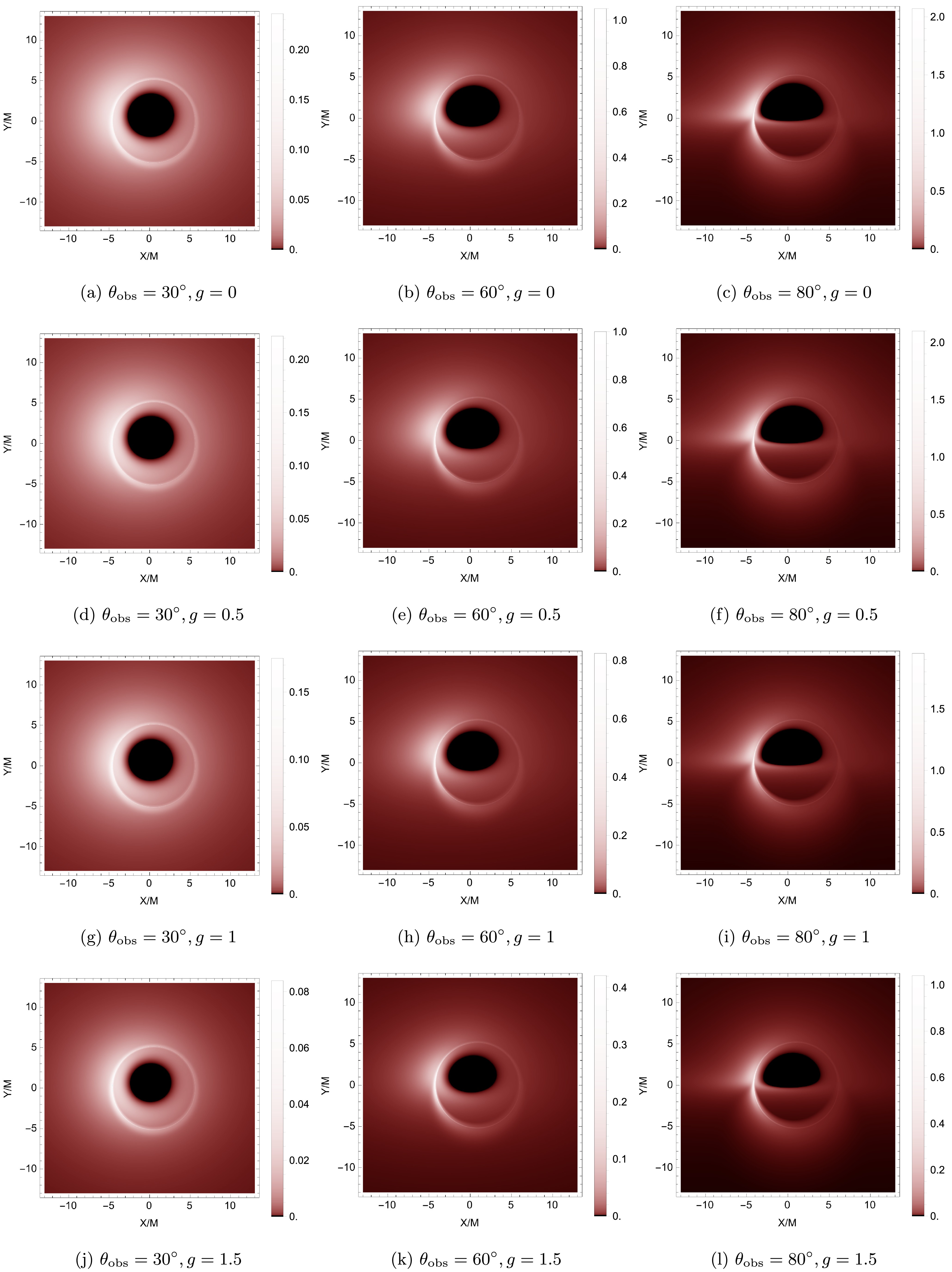
Figure 8. (color online) The optical appearance of a rotating SV black hole with spin parameter
$ a=0.5 $ . From left to right, the observer inclination angles$ \theta_{{\rm{obs}}} $ are$ 30^\circ $ ,$ 60^\circ $ , and$ 80^\circ $ . From top to bottom, the parameter g takes the values$ 0 $ (Kerr case),$ 0.5 $ ,$ 1 $ , and$ 1.5 $ .We emphasize that the parameter range of g considered in Fig. 8 is deliberately restricted to
$ g\leq 1.5 $ . As shown in Fig. 1, for fixed$ a=0.5 $ , the event horizon radius decreases rapidly once$ g\gtrsim 1.5 $ . Consequently, the emission radius relevant to radiative transfer shifts to smaller values, where the emissivity$ j(r_{n}) $ given by Eq. (41) is strongly suppressed, leading to a substantial reduction in the observed intensity$ I_{{\rm{obs}}} $ .For completeness, we computed black hole images for
$ a=0.5 $ and$ g=1.86 $ , which corresponds to the maximal value of g allowed by the regular black hole condition. The resulting images for inclination angles$ \theta_{{\rm{obs}}}=30^\circ $ ,$ 60^\circ $ , and$ 80^\circ $ are shown in Fig. 9. Although the overall intensity is reduced by several orders of magnitude compared with the cases displayed in Fig. 8, the qualitative image structure, including the photon ring and the inner shadow, remains intact. To avoid confusion caused by the drastic change in the chosen intensity model, we therefore restrict our detailed analysis to$ g\leq 1.5 $ henceforth.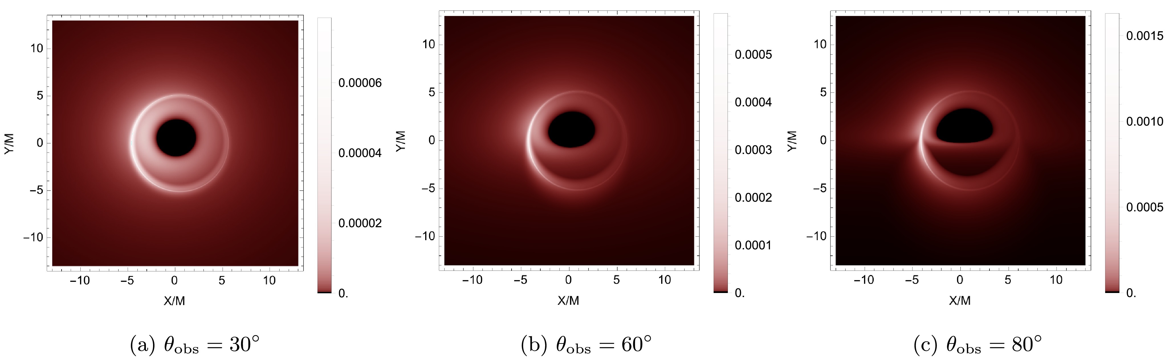
Figure 9. (color online) Optical appearance of a rotating SV black hole with
$ a=0.5 $ and$ g=1.86 $ for different values of the observational inclination angle$ \theta_{{\rm{obs}}} $ . The overall intensity is significantly suppressed compared with those shown in Fig. 8, while the photon ring and inner shadow structures remain clear.Since the optical appearance images provide only a qualitative indication of how the parameter g affects the black hole silhouette, we further examine the influence of g on the observed intensity in a quantitative manner by plotting the intensity profiles on the observer’s screen. In Fig. 10, we consider the intensity distributions along the X- and Y-axes for a Kerr black hole with
$ a=0.5 $ and for a rotating SV black hole with$ a=0.5 $ and$ g=1 $ . Along the X-axis, the observed intensity exhibits two prominent peaks; as the inclination angle increases, the left peak is enhanced while the right peak is suppressed, leading to increasing asymmetry between the two peaks. This behavior is mainly caused by the Doppler effect, which becomes dominant at large inclination angles. Moreover, the presence of the parameter g reduces the observed intensity at almost all screen points, significantly suppressing the peak values and modestly reducing the inner shadow size compared with the Kerr case. Along the Y-axis, three distinct intensity peaks gradually emerge as the inclination angle increases, and their peak intensities are substantially reduced relative to the Kerr black hole case by the parameter g.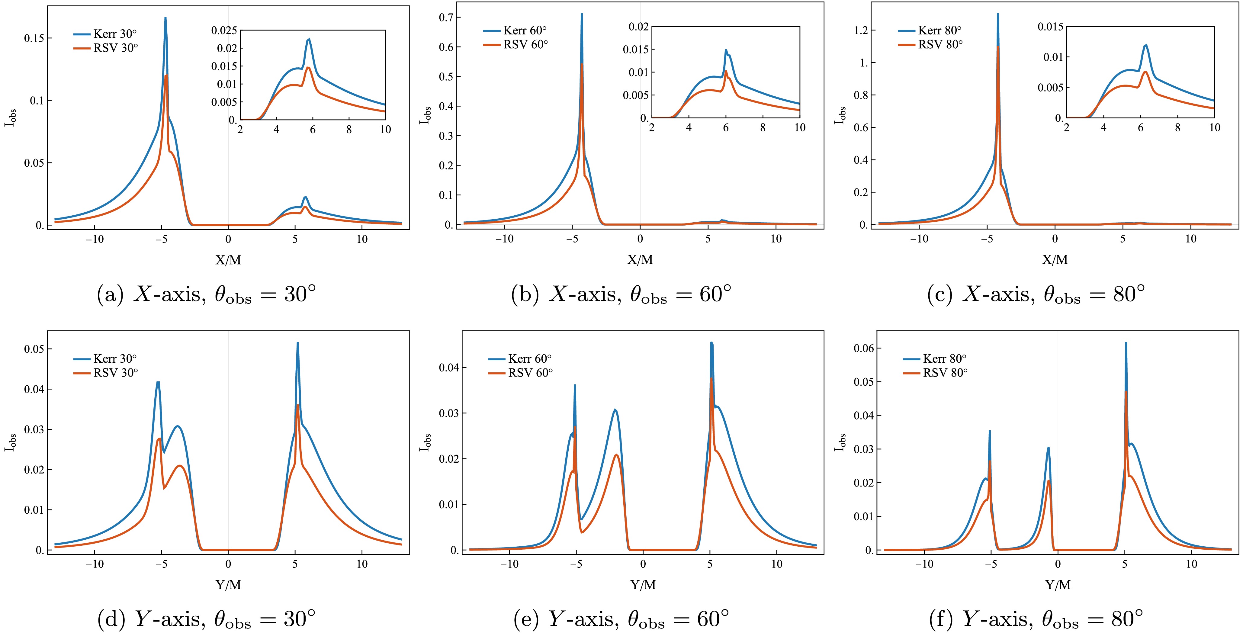
Figure 10. (color online) Observed intensity profiles on the observer’s screen along the X- and Y-axes are shown for a Kerr black hole (
$ a=0.5,\ g=0 $ ) and a rotating SV black hole ($ a=0.5,\ g=1 $ ) at different observer inclination angles. The top row shows the intensity distributions along the X-axis, while the bottom row shows those along the Y-axis.Given the crucial role played by the redshift factor in shaping black hole images, we plot the distribution of the redshift factor associated with the direct image for the same set of parameters as in Fig. 8 (excluding the Kerr case) and present the results in Fig. 11. To visualize the redshift factor more intuitively, we adopt a linear color scale, where red denotes redshifted regions (
$ g<1 $ ) and blue denotes blueshifted regions ($ g>1 $ ). When the observer inclination angle is$ \theta_{{\rm{obs}}}=30^\circ $ , the entire screen is dominated by redshift; for larger inclination angles,$ \theta_{{\rm{obs}}}=60^\circ $ and$ 80^\circ $ , a blueshifted region appears on the left side of the image, enhancing the observed intensity, while the right side remains redshifted and correspondingly dimmer. This behavior is consistent with the increasing asymmetry between the left- and right-hand intensity peaks discussed previously. In addition, as g increases, the overall pattern of redshifted and blueshifted regions remains unchanged; however, the reduction of the inner shadow causes the redshifted area to expand. Moreover, for$ \theta_{{\rm{obs}}}=80^\circ $ , with increasing g, the blueshifted region becomes slightly stronger, leading to a larger intensity contrast in the image.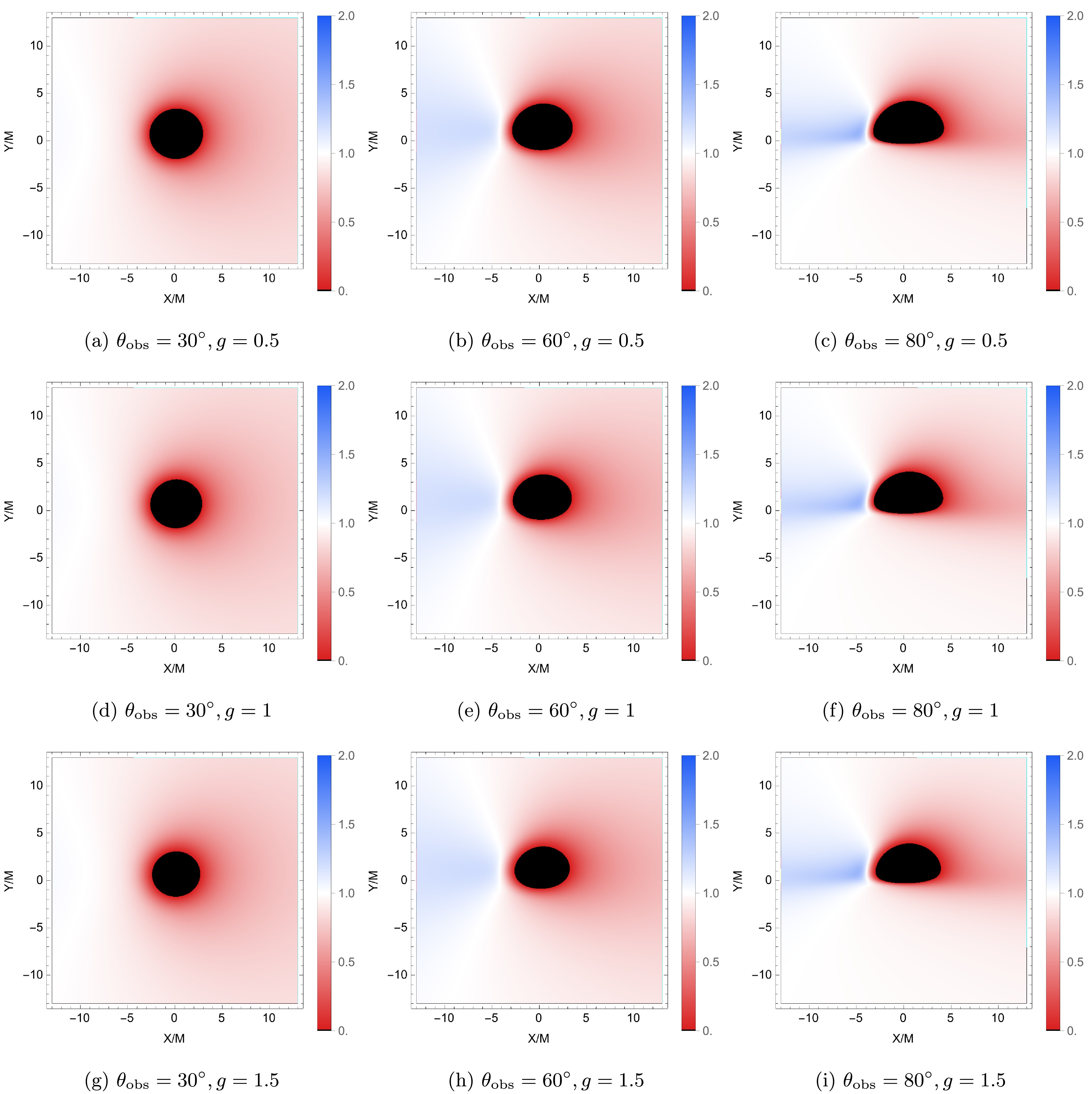
Figure 11. (color online) Distribution of the redshift factor for the direct image of a rotating SV black hole with
$ a=0.5 $ , for various observer inclination angles and values of the parameter g.We then turn to the redshift factor distribution associated with the lensed image, computed using the same parameter set as in the direct image case, and the corresponding results are shown in Fig. 12. In each panel, the boundary of the inner shadow is encircled by a prominent red ring, indicating strong gravitational redshift arising from photons emitted in the plunging region inside the ISCO. Overall, the lensed image is redshift-dominated and, as in the direct image, no blueshifted region appears when the observer inclination angle is
$ \theta_{{\rm{obs}}}=30^\circ $ . However, at larger inclination angles,$ \theta_{{\rm{obs}}}=60^\circ $ or$ 80^\circ $ , a small blueshifted region emerges near the left edge of the inner shadow; this blueshift becomes more pronounced as the parameter g increases. Taken together with the direct-image results, these findings indicate that, at moderate to high inclination angles where blueshifted regions are present, the regularization parameter enhances the blueshift in the observed black hole images.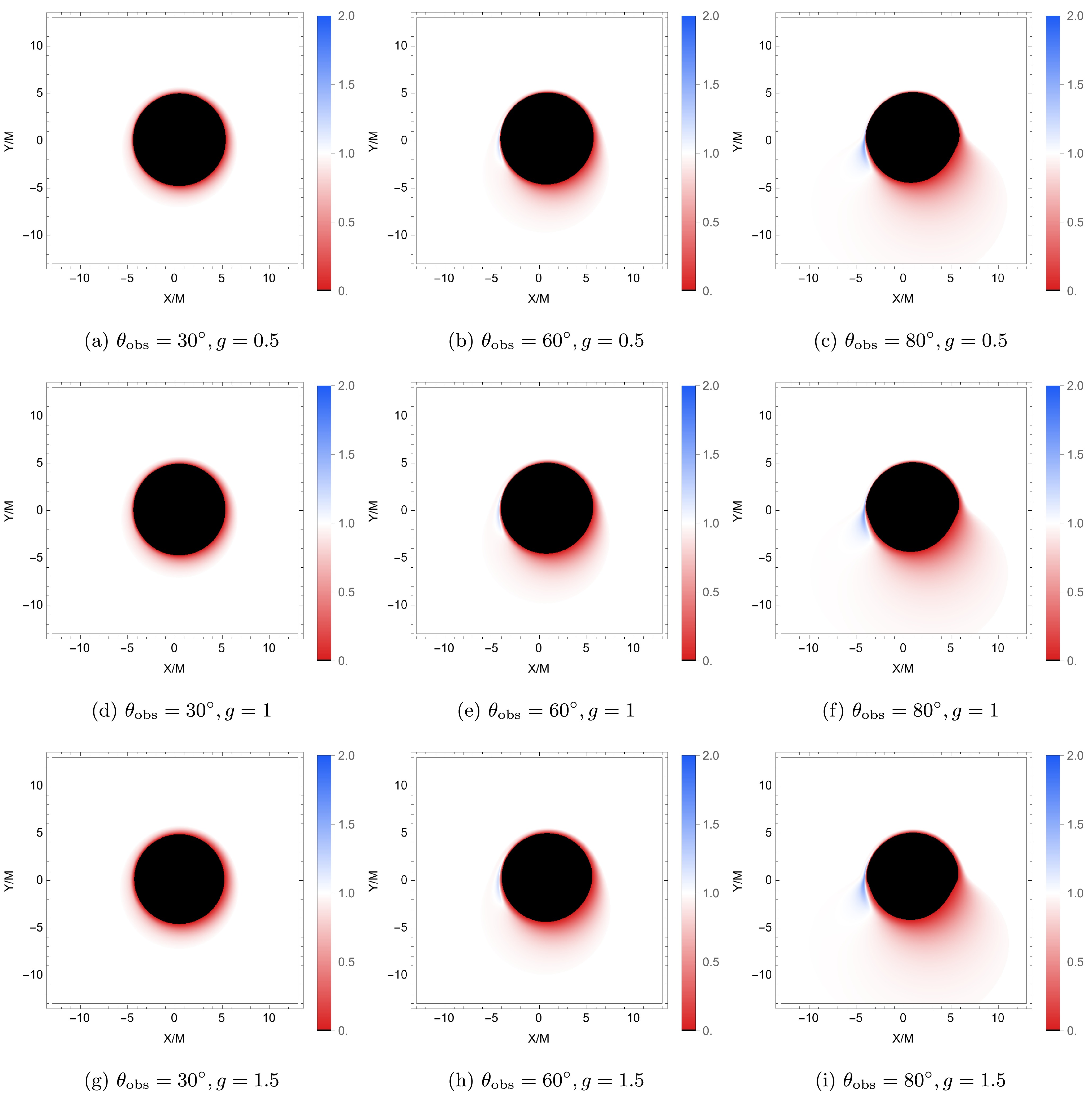
Figure 12. (color online) Distribution of the redshift factor associated with the lensed image of a rotating SV black hole with
$ a=0.5 $ at various observer inclination angles and for different values of the parameter g.To clarify the differences among the direct, lensed, and higher-order images, we plot the observed flux for the same parameter set as above, as shown in Fig. 13. In these subfigures, the thin green bands correspond to the higher-order images, the blue regions represent the lensed images, and the yellow regions denote the direct images, which cover most of the observer’s screen. The central black area indicates the inner shadow of the black hole. When the observer inclination angle is
$ \theta_{{\rm{obs}}}=60^\circ $ or$ 80^\circ $ , the inner shadow develops a characteristic hat-like shape; this feature becomes more pronounced at$ \theta_{{\rm{obs}}}=80^\circ $ . Increasing the inclination angle also significantly enlarges the lensed-image region. Furthermore, as the parameter g increases, the inner shadow shrinks while the lensed-image region expands; notably, the higher-order image also broadens.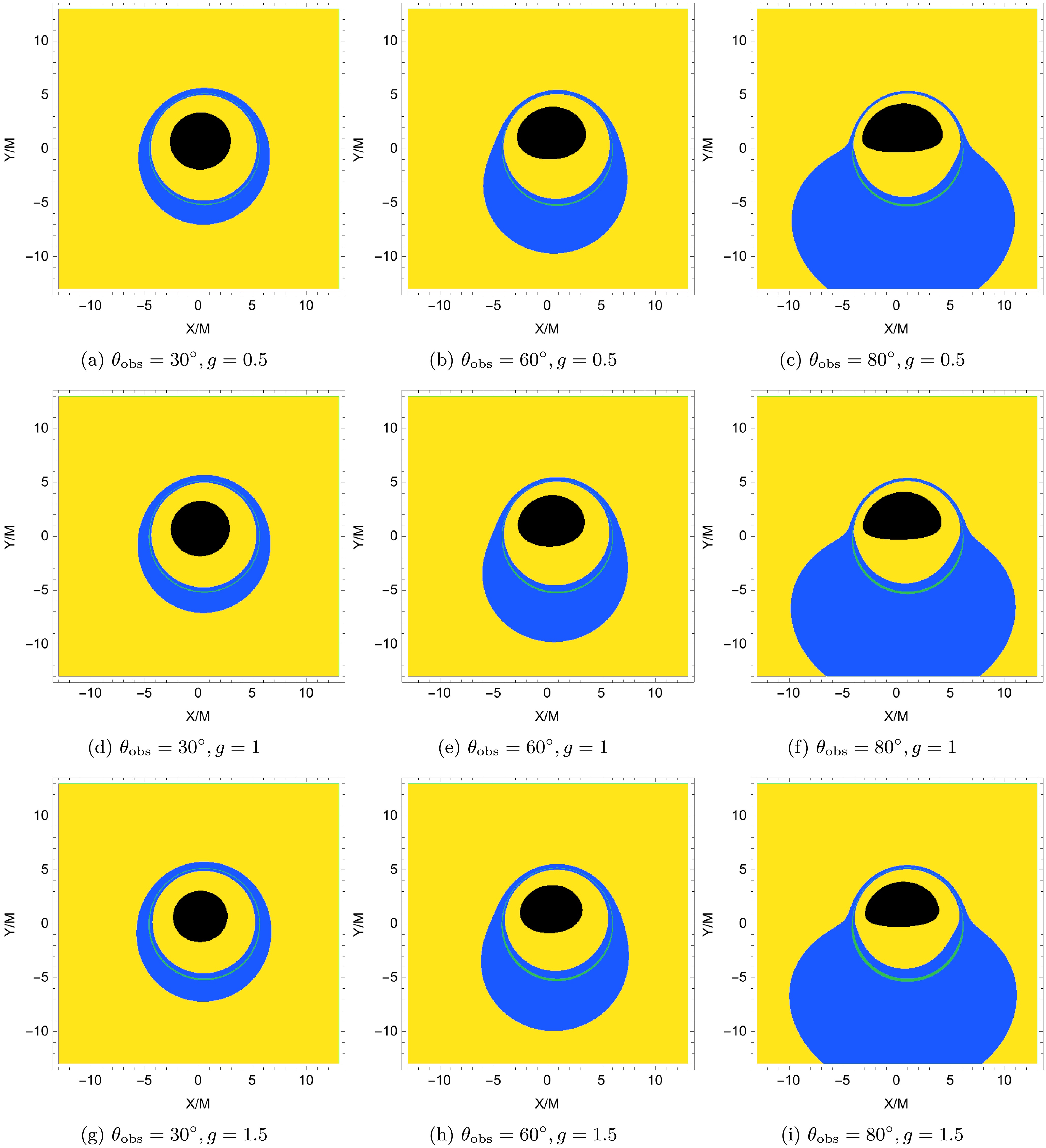
Figure 13. (color online) Observed flux distribution for a rotating SV black hole with
$ a=0.5 $ , for various observer inclination angles and values of the parameter g.Having comprehensively investigated the impact of the regularization parameter g on various aspects of the black hole images (including the optical appearance, redshift factor, and the distribution of different-order images), we now fix
$ g = 0.9 $ and further explore the effect of the spin parameter a on the optical appearance of the rotating SV black hole. The corresponding numerical results are presented in Fig. 14. For the three observer inclination angles$ \theta_{{\rm{obs}}} = 30^\circ $ ,$ 60^\circ $ , and$ 80^\circ $ , increasing a enhances frame dragging and thus light bending, profoundly affecting the images. Specifically, the inner shadow shrinks markedly. Furthermore, the photon ring undergoes strong distortion; in the rapidly spinning case ($ a=0.99 $ ) at a high inclination ($ \theta_{{\rm{obs}}} = 80^\circ $ ), it exhibits a characteristic "D" shape. Although the spin parameter a dominantly shapes the macroscopic appearance of the black hole image, the physical effects induced by g act as nontrivial corrections to these spin-induced deformations. These g-dependent fine-structure features provide crucial clues for distinguishing rotating SV black holes from standard Kerr black holes.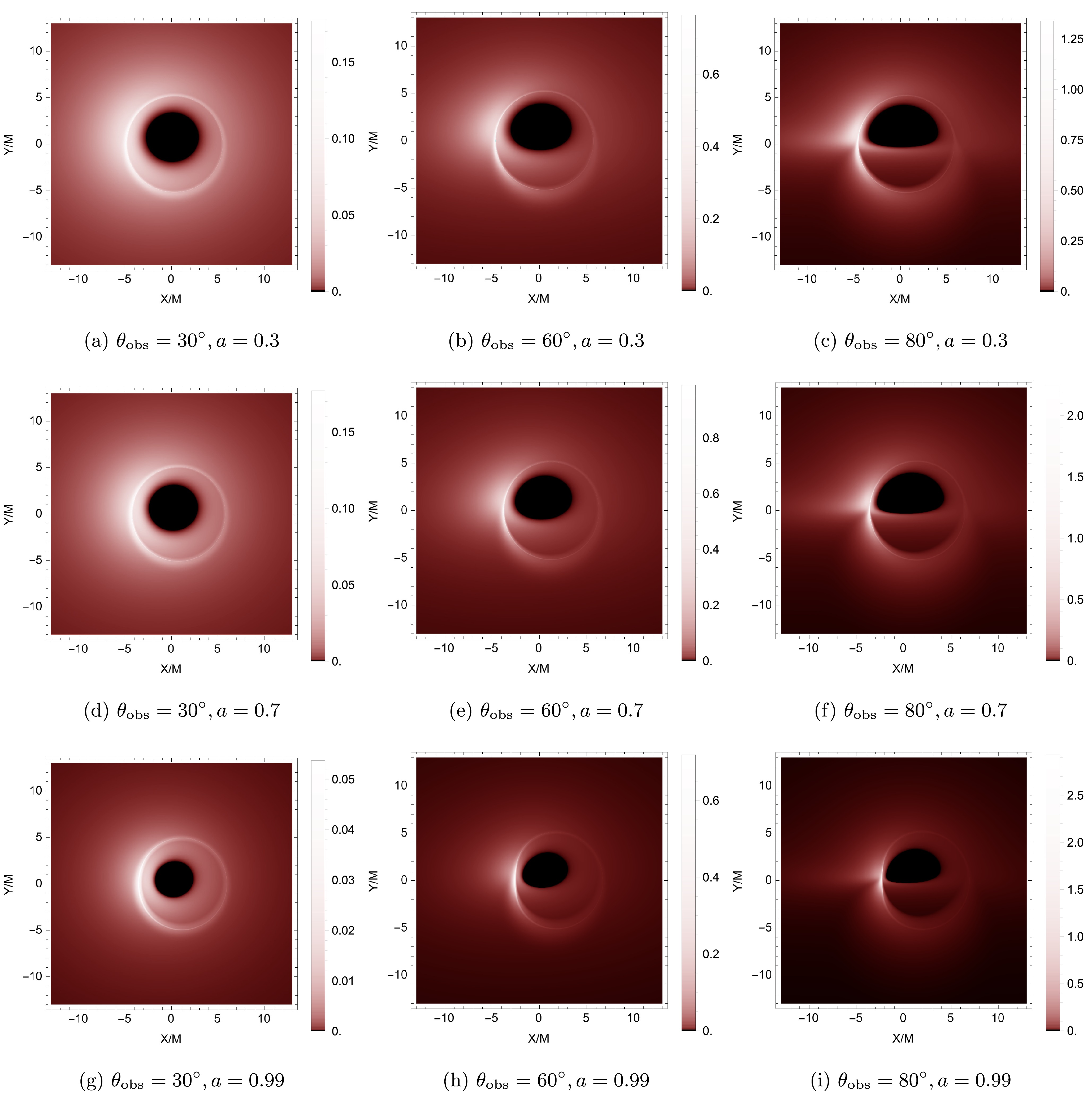
Figure 14. (color online) Optical appearance of a rotating SV black hole with fixed parameter
$ g=0.9 $ . From left to right, the observer inclination angle$ \theta_{{\rm{obs}}} $ is$ 30^\circ $ ,$ 60^\circ $ , and$ 80^\circ $ ; from top to bottom, the spin parameter a is$ 0.3 $ ,$ 0.7 $ , and$ 0.99 $ . -
Having analyzed the radiative properties of thin accretion disks, we now turn to the optical appearance of the rotating SV black hole as seen by a distant observer. To investigate this, we employ ray tracing to determine which photons emitted from the accretion disk reach the observer [89, 90]. Because not all photons originating from the disk can escape to infinity, we adopt a backward ray-tracing approach, in which photon trajectories are traced from the observer’s screen back toward the black hole until it is determined whether they intersect the accretion disk.
The observer’s screen is modeled as a three-dimensional Cartesian coordinate system
$ (X,Y,Z) $ , with the negative Z-axis pointing toward the black hole. The observer is located at a fixed position$ (r_{{\rm{obs}}},\theta_{{\rm{obs}}},\phi_{{\rm{obs}}}) $ in the Boyer–Lindquist coordinate system. In the observer’s frame, the photon’s initial position is taken to be$ (X,Y,0) $ , and its initial spatial velocity is set to$ (0,0,-1) $ , corresponding to photons incident perpendicular to the screen. A crucial step in the ray-tracing procedure is to establish the mapping between the observer’s frame and the black hole frame. Following the literature [90], the Cartesian components$ (x,y,z) $ of the photon’s initial position in the black hole frame are given by$ x = D\cos\phi_{{\rm{obs}}}-X\sin\phi_{{\rm{obs}}}, $
(24) $ y = D\sin\phi_{{\rm{obs}}}+X\cos\phi_{{\rm{obs}}}, $
(25) $ z = r_{{\rm{obs}}}\cos\theta_{{\rm{obs}}}+Y\sin\theta_{{\rm{obs}}}, $
(26) where
$ D=\sin\theta_{{\rm{obs}}}\sqrt{r_{{\rm{obs}}}^{2}+a^{2}}-Y\cos\theta_{{\rm{obs}}}. $
(27) The corresponding Boyer–Lindquist coordinates of the photon's position are then obtained as
$ r =\sqrt{\sigma+\sqrt{\sigma^{2}+a^{2}z^{2}}}, $
(28) $ \theta =\arccos\frac{z}{r}, $
(29) $ \phi =\arctan\frac{y}{x}, $
(30) where
$ \sigma=\frac{x^{2}+y^{2}+z^{2}-a^{2}}{2}. $
(31) Under the same transformation, the spatial components of the photon’s initial velocity in Boyer–Lindquist coordinates are given by
$ \Sigma = r^{2}+a^{2}\cos^{2}\theta,\quad {\cal{R}}=\sqrt{r^{2}+a^{2}},\quad \Phi=\phi-\phi_{{\rm{obs}}}, $
(32) $ \dot r = -\frac{1}{\Sigma} \left[r{\cal{R}}\sin\theta\sin\theta_{{\rm{obs}}}\cos\Phi + {\cal{R}}^{2}\cos\theta\cos\theta_{{\rm{obs}}}\right], $
(33) $ \dot\theta = -\frac{1}{\Sigma} \left[{\cal{R}}\cos\theta\sin\theta_{{\rm{obs}}}\cos\Phi - r\sin\theta\cos\theta_{{\rm{obs}}}\right], $
(34) $ \dot\phi = \frac{1}{{\cal{R}}}\sin\theta_{{\rm{obs}}}\sin\Phi\,\csc\theta . $
(35) Without loss of generality, we set the photon's initial time coordinate to
$ t=0 $ , and determine its temporal velocity component from the geodesic constraint.$ \beta=-\frac{g_{t\phi}\dot\phi}{g_{tt}},\qquad \aleph=\frac{\delta-g_{ij}\dot x^{i}\dot x^{j}}{g_{tt}},\qquad \dot t=\beta+\sqrt{\beta^{2}+\aleph}, $
(36) where
$ \delta=0 $ for photons, and the spatial indices run over$ i,j=r,\theta,\phi $ . Once the initial position and four-velocity of a photon are specified, the canonical momentum is obtained via the transformation$ p_\mu = g_{\mu\nu}\dot x^\nu . $
(37) Photon propagation in the rotating regular black-hole spacetime is then governed by Hamilton's equations.
$ \dot x^\mu=\frac{\partial {\cal{H}}}{\partial p_\mu},\qquad \dot p_\mu=-\frac{\partial {\cal{H}}}{\partial x^\mu}, $
(38) with the Hamiltonian
$ {\cal{H}}=\frac{1}{2}g^{\mu\nu}p_\mu p_\nu=0, $
(39) These equations correspond to the null geodesics of photons. By numerically integrating them, one can reconstruct complete photon trajectories and determine whether they intersect the accretion disk, thereby producing the optical image observed by a distant observer.
The observed specific intensity,
$ I_{{\rm{obs}}} $ , can be expressed as a sum over multiple intersections of photon trajectories with the accretion disk. Following the radiative GRMHD imaging prescription, it is given by [91−95]$ I_{{\rm{obs}}}=\sum\limits_{n=1}^{N_{\max}} f_n\, g_{n}^3\, j(r_n), $
(40) where n denotes the number of times a photon trajectory intersects the accretion disk. Since higher-order crossings contribute negligibly to the observed intensity, we truncate the sum at
$ N_{\max}=3 $ . Specifically,$ n=1 $ corresponds to the direct image,$ n=2 $ to the lensed image, and$ n=3 $ to the higher-order image. The coefficients$ f_n $ are phenomenological weighting factors that account for the relative contributions of different image orders. In this work, we adopt$ f_1=1 $ and$ f_2=f_3=\frac{2}{3} $ . The function$ j(r_n) $ denotes the emissivity of the accretion disk and depends on the radial coordinate$ r_n $ of the emission point. The emissivity can be expressed as [91]:$ j(r_n)=\exp\left(p_1 i+p_2 i^2\right), $
(41) where
$ i = \log(r_{n}/r_{+}) $ . For the$ 230\,{\rm{GHz}} $ imaging simulations, the parameters are set to$ p_1=-2 $ and$ p_2=-\tfrac{1}{2} $ . Finally,$ g_{n} $ is the redshift factor that relates the emitted frequency to the observed frequency.$ g_{n}=\frac{\nu_{{\rm{obs}}}}{\nu_e} =\frac{(p_\mu u^\mu)_{{\rm{obs}}}}{(p_\mu u^\mu)_e}, $
(42) where
$ p^\mu $ is the photon four-momentum and$ u^\mu $ denotes the four-velocity of the observer or of the emitting matter in the accretion disk, as appropriate.It should be emphasized that the redshift factor takes different forms inside and outside the innermost stable circular orbit. For photon emission originating in the region
$ r>r_{{\rm{ISCO}}} $ , we assume that the accretion flow follows stable circular orbits in the equatorial plane. Consequently, the redshift factor is given by$ g_{n} = g_{{\rm{out}}} =\frac{p_t}{u^t\left(p_t+\Omega p_\phi\right)} . $
(43) In the previous section, the redshift factor entering the spectral-luminosity formula was approximated by
$ g_{{\rm{out}}} $ , which is sufficient for computing the spectral luminosity since the dominant contribution arises from regions outside the ISCO. In contrast, for emission from the plunging region$ r_+<r<r_{{\rm{ISCO}}} $ , the accretion flow no longer follows circular orbits. Following the standard approach in [84, 96], we assume that the particles' specific energy and specific angular momentum are conserved during the plunge and retain their ISCO values, i.e.,$ E=E_{{\rm{ISCO}}} $ and$ L=L_{{\rm{ISCO}}} $ . In this region, the redshift factor is evaluated as$ g_{n} = g_{{\rm{in}}} =\frac{p_t}{u^t_{{\rm{in}}} p_t + u^r_{{\rm{in}}} p_r + u^\phi_{{\rm{in}}} p_\phi}, $
(44) where
$ u^t_{{\rm{in}}} $ ,$ u^r_{{\rm{in}}} $ , and$ u^\phi_{{\rm{in}}} $ denote the four-velocity components of the infalling matter, with the parameters E and L replaced by$ E_{{\rm{ISCO}}} $ and$ L_{{\rm{ISCO}}} $ , respectively. With these inputs, the black hole image on the observer’s screen can be constructed.We fix
$ a=0.5 $ and present the optical appearance of the rotating SV black hole for different values of the parameter g and different observer inclination angles in Fig. 8. In each image, a prominent, bright photon ring appears as a narrow, luminous curve, which is a direct consequence of strong gravitational lensing in the vicinity of the black hole. In addition, a central dark region is clearly visible in each image, corresponding to photons that fall into the event horizon in the backward ray-tracing method. This feature represents the direct imaging of the event horizon and is commonly referred to as the black hole shadow. The three images in the first row correspond to the Kerr black hole case with$ g=0 $ and observer inclination angles of$ 30^\circ $ ,$ 60^\circ $ , and$ 80^\circ $ , while the subsequent rows, from top to bottom, correspond to$ g=0.5 $ ,$ 1 $ , and$ 1.5 $ , respectively. As g increases, the size of the inner shadow decreases noticeably and the overall image brightness is suppressed, indicating that the regularization parameter modifies the near-horizon spacetime geometry.
Figure 8. (color online) The optical appearance of a rotating SV black hole with spin parameter
$ a=0.5 $ . From left to right, the observer inclination angles$ \theta_{{\rm{obs}}} $ are$ 30^\circ $ ,$ 60^\circ $ , and$ 80^\circ $ . From top to bottom, the parameter g takes the values$ 0 $ (Kerr case),$ 0.5 $ ,$ 1 $ , and$ 1.5 $ .We emphasize that the parameter range of g considered in Fig. 8 is deliberately restricted to
$ g\leq 1.5 $ . As shown in Fig. 1, for fixed$ a=0.5 $ , the event horizon radius decreases rapidly once$ g\gtrsim 1.5 $ . Consequently, the emission radius relevant to radiative transfer shifts to smaller values, where the emissivity$ j(r_{n}) $ given by Eq. (41) is strongly suppressed, leading to a substantial reduction in the observed intensity$ I_{{\rm{obs}}} $ .For completeness, we computed black hole images for
$ a=0.5 $ and$ g=1.86 $ , which corresponds to the maximal value of g allowed by the regular black hole condition. The resulting images for inclination angles$ \theta_{{\rm{obs}}}=30^\circ $ ,$ 60^\circ $ , and$ 80^\circ $ are shown in Fig. 9. Although the overall intensity is reduced by several orders of magnitude compared with the cases displayed in Fig. 8, the qualitative image structure, including the photon ring and the inner shadow, remains intact. To avoid confusion caused by the drastic change in the chosen intensity model, we therefore restrict our detailed analysis to$ g\leq 1.5 $ henceforth.
Figure 9. (color online) Optical appearance of a rotating SV black hole with
$ a=0.5 $ and$ g=1.86 $ for different values of the observational inclination angle$ \theta_{{\rm{obs}}} $ . The overall intensity is significantly suppressed compared with those shown in Fig. 8, while the photon ring and inner shadow structures remain clear.Since the optical appearance images provide only a qualitative indication of how the parameter g affects the black hole silhouette, we further examine the influence of g on the observed intensity in a quantitative manner by plotting the intensity profiles on the observer’s screen. In Fig. 10, we consider the intensity distributions along the X- and Y-axes for a Kerr black hole with
$ a=0.5 $ and for a rotating SV black hole with$ a=0.5 $ and$ g=1 $ . Along the X-axis, the observed intensity exhibits two prominent peaks; as the inclination angle increases, the left peak is enhanced while the right peak is suppressed, leading to increasing asymmetry between the two peaks. This behavior is mainly caused by the Doppler effect, which becomes dominant at large inclination angles. Moreover, the presence of the parameter g reduces the observed intensity at almost all screen points, significantly suppressing the peak values and modestly reducing the inner shadow size compared with the Kerr case. Along the Y-axis, three distinct intensity peaks gradually emerge as the inclination angle increases, and their peak intensities are substantially reduced relative to the Kerr black hole case by the parameter g.
Figure 10. (color online) Observed intensity profiles on the observer’s screen along the X- and Y-axes are shown for a Kerr black hole (
$ a=0.5,\ g=0 $ ) and a rotating SV black hole ($ a=0.5,\ g=1 $ ) at different observer inclination angles. The top row shows the intensity distributions along the X-axis, while the bottom row shows those along the Y-axis.Given the crucial role played by the redshift factor in shaping black hole images, we plot the distribution of the redshift factor associated with the direct image for the same set of parameters as in Fig. 8 (excluding the Kerr case) and present the results in Fig. 11. To visualize the redshift factor more intuitively, we adopt a linear color scale, where red denotes redshifted regions (
$ g<1 $ ) and blue denotes blueshifted regions ($ g>1 $ ). When the observer inclination angle is$ \theta_{{\rm{obs}}}=30^\circ $ , the entire screen is dominated by redshift; for larger inclination angles,$ \theta_{{\rm{obs}}}=60^\circ $ and$ 80^\circ $ , a blueshifted region appears on the left side of the image, enhancing the observed intensity, while the right side remains redshifted and correspondingly dimmer. This behavior is consistent with the increasing asymmetry between the left- and right-hand intensity peaks discussed previously. In addition, as g increases, the overall pattern of redshifted and blueshifted regions remains unchanged; however, the reduction of the inner shadow causes the redshifted area to expand. Moreover, for$ \theta_{{\rm{obs}}}=80^\circ $ , with increasing g, the blueshifted region becomes slightly stronger, leading to a larger intensity contrast in the image.
Figure 11. (color online) Distribution of the redshift factor for the direct image of a rotating SV black hole with
$ a=0.5 $ , for various observer inclination angles and values of the parameter g.We then turn to the redshift factor distribution associated with the lensed image, computed using the same parameter set as in the direct image case, and the corresponding results are shown in Fig. 12. In each panel, the boundary of the inner shadow is encircled by a prominent red ring, indicating strong gravitational redshift arising from photons emitted in the plunging region inside the ISCO. Overall, the lensed image is redshift-dominated and, as in the direct image, no blueshifted region appears when the observer inclination angle is
$ \theta_{{\rm{obs}}}=30^\circ $ . However, at larger inclination angles,$ \theta_{{\rm{obs}}}=60^\circ $ or$ 80^\circ $ , a small blueshifted region emerges near the left edge of the inner shadow; this blueshift becomes more pronounced as the parameter g increases. Taken together with the direct-image results, these findings indicate that, at moderate to high inclination angles where blueshifted regions are present, the regularization parameter enhances the blueshift in the observed black hole images.
Figure 12. (color online) Distribution of the redshift factor associated with the lensed image of a rotating SV black hole with
$ a=0.5 $ at various observer inclination angles and for different values of the parameter g.To clarify the differences among the direct, lensed, and higher-order images, we plot the observed flux for the same parameter set as above, as shown in Fig. 13. In these subfigures, the thin green bands correspond to the higher-order images, the blue regions represent the lensed images, and the yellow regions denote the direct images, which cover most of the observer’s screen. The central black area indicates the inner shadow of the black hole. When the observer inclination angle is
$ \theta_{{\rm{obs}}}=60^\circ $ or$ 80^\circ $ , the inner shadow develops a characteristic hat-like shape; this feature becomes more pronounced at$ \theta_{{\rm{obs}}}=80^\circ $ . Increasing the inclination angle also significantly enlarges the lensed-image region. Furthermore, as the parameter g increases, the inner shadow shrinks while the lensed-image region expands; notably, the higher-order image also broadens.
Figure 13. (color online) Observed flux distribution for a rotating SV black hole with
$ a=0.5 $ , for various observer inclination angles and values of the parameter g.Having comprehensively investigated the impact of the regularization parameter g on various aspects of the black hole images (including the optical appearance, redshift factor, and the distribution of different-order images), we now fix
$ g = 0.9 $ and further explore the effect of the spin parameter a on the optical appearance of the rotating SV black hole. The corresponding numerical results are presented in Fig. 14. For the three observer inclination angles$ \theta_{{\rm{obs}}} = 30^\circ $ ,$ 60^\circ $ , and$ 80^\circ $ , increasing a enhances frame dragging and thus light bending, profoundly affecting the images. Specifically, the inner shadow shrinks markedly. Furthermore, the photon ring undergoes strong distortion; in the rapidly spinning case ($ a=0.99 $ ) at a high inclination ($ \theta_{{\rm{obs}}} = 80^\circ $ ), it exhibits a characteristic "D" shape. Although the spin parameter a dominantly shapes the macroscopic appearance of the black hole image, the physical effects induced by g act as nontrivial corrections to these spin-induced deformations. These g-dependent fine-structure features provide crucial clues for distinguishing rotating SV black holes from standard Kerr black holes.
Figure 14. (color online) Optical appearance of a rotating SV black hole with fixed parameter
$ g=0.9 $ . From left to right, the observer inclination angle$ \theta_{{\rm{obs}}} $ is$ 30^\circ $ ,$ 60^\circ $ , and$ 80^\circ $ ; from top to bottom, the spin parameter a is$ 0.3 $ ,$ 0.7 $ , and$ 0.99 $ . -
In this work, we carry out a study of the electromagnetic properties of the rotating SV black hole with an equatorial thin accretion disk, focusing on the radiative properties and optical appearance of the black hole system. By combining analytical calculations and extensive numerical simulations, we systematically explore how the spin parameter a and the regularization parameter g affect both the emission of the accretion disk and the observed images.
For test particles moving on circular orbits in the equatorial plane of the rotating SV black hole, the ISCO radius is obtained numerically and decreases as the regularization parameter g increases. Interestingly, although the parameter g affects the radial profiles of the specific energy E, angular momentum L, angular velocity Ω, and the ISCO radius, we find that the values of E, L, and Ω evaluated at the ISCO are independent of g. As a direct consequence, the radiative efficiency of the rotating SV black hole is the same as that of the corresponding Kerr black hole.
Although the radiative efficiency of the rotating SV black hole is not affected by the regularization parameter g, other radiative properties of a thin accretion disk around the rotating SV black hole do depend on g. The dimensionless radiative flux and effective temperature of the accretion disk are computed numerically and presented for different values of the parameters g and a. It is found that, for an SV black hole with fixed g, the influence of the parameter a on these local quantities is qualitatively the same as in the Kerr case, and both quantities are enhanced as a increases. In contrast, the regularization parameter g suppresses the peak values of the radiative flux and effective temperature. Using observationally motivated parameters for Sgr A
$ ^{*} $ and M87$ ^{*} $ , we present two concrete examples to show the influence of g on the peak values of the radiative flux and effective temperature. The peak value of the radiative flux decreases by about 4% and 6% for$ g=1.86,\; a=0.5 $ and$ g=1.5, a=0.8 $ , respectively. We also observe that the suppression effect of the regularization parameter g is more pronounced for higher-spin black holes. Besides these local quantities, we also incorporate the redshift factor for a distant observer with zero inclination and compute the spectral luminosity for different parameters. Our results indicate that the spin parameter a significantly enhances the spectral luminosity, whereas the effect of g is comparatively weaker. In particular, for$ a=0.5 $ , the spectral luminosity of the Kerr black hole is approximately$ 1.01 $ times that of the rotating SV black hole with$ g=1.86 $ .By employing a backward ray-tracing technique, we numerically simulate the optical appearance of rotating SV black holes for different inclination angles and model parameters. We also compare the intensity profiles along the X- and Y-axes on the observer's screen between a Kerr black hole with
$ a=0.5 $ and a rotating SV black hole with$ a=0.5 $ and$ g=1 $ . An increase in g leads to an overall suppression of the observed intensity and a noticeable reduction in the inner shadow size.In addition, we plot the distribution of the redshift factor for both direct and lensed images. The regularization parameter g slightly enhances the blueshifted regions in both images, and this enhancement is more evident for observers at large inclination angles (e.g.,
$ 60^\circ $ or$ 80^\circ $ ). Furthermore, we also consider the direct, lensed, and higher-order images of the observed flux distribution. Although the inclination angle affects this distribution significantly, as expected, we find that increasing g leads to a noticeable increase in the width of the photon ring region. This implies that more refined structures may be more sensitive to the regularization parameter g. Thus, in order to test possible deviations from the Kerr hypothesis for astrophysical black holes, optimal observational targets are systems with higher spin and larger inclination angle, and observations of their higher-order structures are also crucial. For the sake of completeness, we also investigate the impact of the spin parameter a on the optical appearance of the rotating SV black hole. Although the effect of the spin parameter a is substantially more pronounced, the nontrivial corrections introduced by the regularization parameter g to these rotation-induced effects provide a crucial opportunity to distinguish rotating SV black holes from standard Kerr black holes.The results presented in [41] highlight a degeneracy between rotating SV black holes and Kerr black holes at the level of shadow size. Our analysis demonstrates that accretion-disk-related observables, including radiative fluxes, spectral luminosities, redshift factors, and observed flux distributions, provide complementary information to break this degeneracy. These findings offer valuable theoretical guidance for future high-resolution observations and may help to distinguish rotating SV black holes from Kerr black holes, thereby shedding light on the possible existence of regular black holes and deepening our understanding of singularity theorems in strong-gravity regimes.
There are several directions for future research. In this work, we focus on the rotating SV black hole with a thin accretion disk, and one may further consider the rotating SV black hole surrounded by a dark matter halo or a thick disk [97−107] and investigate the influence of the regularization parameter on related observables. Another interesting topic is to consider the polarization images and patterns of the accretion flow around the rotating SV black hole, especially in the near-horizon region, which can be used to probe the black hole geometry [96, 108−115]. These further studies may shed more light on distinguishing the rotating SV black hole from the corresponding Kerr black hole.
-
In this work, we carry out a study of the electromagnetic properties of the rotating SV black hole with an equatorial thin accretion disk, focusing on the radiative properties and optical appearance of the black hole system. By combining analytical calculations and extensive numerical simulations, we systematically explore how the spin parameter a and the regularization parameter g affect both the emission of the accretion disk and the observed images.
For test particles moving on circular orbits in the equatorial plane of the rotating SV black hole, the ISCO radius is obtained numerically and decreases as the regularization parameter g increases. Interestingly, although the parameter g affects the radial profiles of the specific energy E, angular momentum L, angular velocity Ω, and the ISCO radius, we find that the values of E, L, and Ω evaluated at the ISCO are independent of g. As a direct consequence, the radiative efficiency of the rotating SV black hole is the same as that of the corresponding Kerr black hole.
Although the radiative efficiency of the rotating SV black hole is not affected by the regularization parameter g, other radiative properties of a thin accretion disk around the rotating SV black hole do depend on g. The dimensionless radiative flux and effective temperature of the accretion disk are computed numerically and presented for different values of the parameters g and a. It is found that, for an SV black hole with fixed g, the influence of the parameter a on these local quantities is qualitatively the same as in the Kerr case, and both quantities are enhanced as a increases. In contrast, the regularization parameter g suppresses the peak values of the radiative flux and effective temperature. Using observationally motivated parameters for Sgr A
$ ^{*} $ and M87$ ^{*} $ , we present two concrete examples to show the influence of g on the peak values of the radiative flux and effective temperature. The peak value of the radiative flux decreases by about 4% and 6% for$ g=1.86,\; a=0.5 $ and$ g=1.5,\; a=0.8 $ , respectively. We also observe that the suppression effect of the regularization parameter g is more pronounced for higher-spin black holes. Besides these local quantities, we also incorporate the redshift factor for a distant observer with zero inclination and compute the spectral luminosity for different parameters. Our results indicate that the spin parameter a significantly enhances the spectral luminosity, whereas the effect of g is comparatively weaker. In particular, for$ a=0.5 $ , the spectral luminosity of the Kerr black hole is approximately$ 1.01 $ times that of the rotating SV black hole with$ g=1.86 $ .By employing a backward ray-tracing technique, we numerically simulate the optical appearance of rotating SV black holes for different inclination angles and model parameters. We also compare the intensity profiles along the X- and Y-axes on the observer's screen between a Kerr black hole with
$ a=0.5 $ and a rotating SV black hole with$ a=0.5 $ and$ g=1 $ . An increase in g leads to an overall suppression of the observed intensity and a noticeable reduction in the inner shadow size.In addition, we plot the distribution of the redshift factor for both direct and lensed images. The regularization parameter g slightly enhances the blueshifted regions in both images, and this enhancement is more evident for observers at large inclination angles (e.g.,
$ 60^\circ $ or$ 80^\circ $ ). Furthermore, we also consider the direct, lensed, and higher-order images of the observed flux distribution. Although the inclination angle affects this distribution significantly, as expected, we find that increasing g leads to a noticeable increase in the width of the photon ring region. This implies that more refined structures may be more sensitive to the regularization parameter g. Thus, in order to test possible deviations from the Kerr hypothesis for astrophysical black holes, optimal observational targets are systems with higher spin and larger inclination angle, and observations of their higher-order structures are also crucial. For the sake of completeness, we also investigate the impact of the spin parameter a on the optical appearance of the rotating SV black hole. Although the effect of the spin parameter a is substantially more pronounced, the nontrivial corrections introduced by the regularization parameter g to these rotation-induced effects provide a crucial opportunity to distinguish rotating SV black holes from standard Kerr black holes.The results presented in [41] highlight a degeneracy between rotating SV black holes and Kerr black holes at the level of shadow size. Our analysis demonstrates that accretion-disk-related observables, including radiative fluxes, spectral luminosities, redshift factors, and observed flux distributions, provide complementary information to break this degeneracy. These findings offer valuable theoretical guidance for future high-resolution observations and may help to distinguish rotating SV black holes from Kerr black holes, thereby shedding light on the possible existence of regular black holes and deepening our understanding of singularity theorems in strong-gravity regimes.
There are several directions for future research. In this work, we focus on the rotating SV black hole with a thin accretion disk, and one may further consider the rotating SV black hole surrounded by a dark matter halo or a thick disk [97−107] and investigate the influence of the regularization parameter on related observables. Another interesting topic is to consider the polarization images and patterns of the accretion flow around the rotating SV black hole, especially in the near-horizon region, which can be used to probe the black hole geometry [96, 108−115]. These further studies may shed more light on distinguishing the rotating SV black hole from the corresponding Kerr black hole.
Circular orbits and observational features of the rotating Simpson-Visser black hole surrounded by a thin accretion disk
- Received Date: 2026-03-18
- Available Online: 2026-07-15
Abstract: Since the Event Horizon Telescope (EHT) collaboration released horizon-scale images of the supermassive black holes Sgr A* and M87*, a new observational window for probing black hole spacetimes in the strong-gravity regime has opened. As an important class of Kerr black hole mimickers, rotating Simpson-Visser (SV) black holes exhibit a degeneracy with Kerr black holes in terms of shadow size, making them difficult to distinguish using shadow observations alone. Motivated by this issue, we present a systematic investigation of the radiative properties and optical appearance of rotating SV black holes surrounded by a thin accretion disk, focusing on the influence of the regularization parameter g on the relevant observables. The results show that although the kinematic quantities and the location of the innermost stable circular orbit (ISCO) depend on the regularization parameter g, the radiative efficiency of the rotating SV black hole is the same as that of its Kerr counterpart. Within the Novikov-Thorne thin-disk model, we study the radiative flux, effective temperature, and spectral luminosity; adopting observational parameters relevant to Sgr A* and M87*, we compute concrete examples for rotating SV black holes and compare them with those for Kerr black holes. The results show that the parameter g suppresses the maximum values of these quantities. In addition, using a backward ray-tracing technique, we numerically simulate the optical appearance of rotating SV black holes and analyze the corresponding intensity images, redshift, and observed flux distributions. Our results indicate that these quantities are sensitive to g. In particular, as g increases, the observed intensity is significantly suppressed, and the photon ring region exhibits a remarkable increase in width. Our findings suggest that accretion-disk-related observables may provide important avenues to distinguish between rotating SV black holes and Kerr black holes, and offer theoretical guidance for future high-resolution observations.


 DownLoad: