


 Abstract
 HTML
HTML Reference
 Related
 PDF
PDF


-
Neutron-capture reactions play a crucial role in understanding the stellar evolution and origin of elements in the universe [1, 2]. Over recent decades, great efforts have been made to study these processes, and many important advances have been achieved; however, some uncertainties and unresolved problems remain, especially for the nucleosynthesis of elements heavier than iron [3, 4]. The primary mechanism for producing heavier elements in the universe is the neutron-capture process, mainly the slow neutron-capture process (s-process) and rapid neutron-capture process (r-process). The s-process proceeds around the β-stability valley, while the r-process takes place in the very neutron-rich region involving many short-lived unknown nuclei.
Experimentally, neutron-capture reactions have mainly been studied for nuclei near the β-stability valley. Recent measurements include the 165Ho(n, γ)166Ho cross section measured using total energy detection systems [5] and 176Yb(n, γ)177Yb cross section using the time-of-flight technique [6]. However, many nuclei involved in the r-process are located in the unknown neutron-rich region, making the measurements of their neutron-capture cross sections extremely challenging. Some indirect methods have also been developed to measure neutron-capture cross sections, such as the surrogate reaction method [7], γ-ray strength function method [8, 9], Oslo method [10, 11], and β-Oslo method [12]. Recently, measurements of neutron-capture cross sections have achieved great progress, such as the 66Ni(n, γ)67Ni cross section using the inverse-Oslo method [13], 92Sr(n, γ)93Sr cross section using the β-Oslo method [14], and 233Pa(n, γ)234Pa cross section using the surrogate reaction method [15].
Theoretically, the neutron-capture reaction cross sections are mainly predicted by the Hauser–Feshbach statistical model [16], and some code packages have been developed based on the statistical model, such as the famous TALYS [17, 18], NON-SMOKER [19], EMPIRE [20], and CCONE [21]. However, there are large differences among different Hauser–Feshbach calculations, especially in the unknown region, which comes mainly from the Hauser–Feshbach model parameters, including the level density, gamma strength function, and optical model [22, 23]. By varying all 9 different reaction models to find the optimal results, a TENDL-astro 2023 library was constructed based on the TALYS-1.96 nuclear reaction code, which provides a highly accurate description of the experimental MACS data [24]. The empirical formula is also widely used to predict various nuclear properties with very low computational cost, such as nuclear masses [25−28], α-decay half-lives [29−32], and β-decays half-lives [33, 34]. The empirical formula for MACS can be obtained by approximating the theoretical calculations [35]; however, its accuracy is far from the requirements for the r-process studies. Recently, several empirical formulas have been developed to predict MACS of the neutron-capture reaction with an accuracy comparable to that of the Hauser–Feshbach statistical model for known data [23, 36, 37].
In recent years, machine learning (ML) has found widespread applications in physics [38], including particle physics [39−41], condensed matter physics [42, 43], and astrophysics [44, 45]. In nuclear physics, there are many ML applications that improve the description of various nuclear properties [46], e.g., nuclear masses [47−52], α and β-decay half-lives [53−57], charge radii [58, 59], low-lying excited states [60−63], neutron-induced fission cross sections [64], and fission yields [65, 66]. ML methods have also been applied to the study of many nuclear reactions, e.g., (n, 2n) reaction cross sections [67], (
$ n,\gamma $ ) reaction cross sections [68], isotopic cross sections in proton induced spallation reactions [69], (n, p) reaction cross sections [70], and (n, α) reaction cross sections [71]. Other ML applications include applications in variational calculations [72, 73], the construction of nuclear energy density functionals [74], and extrapolations for many-body physics [75−78].The physically interpretable or physics-informed ML methods can combine the advantages of ML and nuclear models to improve the performance, robustness, and interpretability of nuclear property predictions [79, 80]. One can also use ML methods to estimate physics-unconstrained parameters of nuclear models, thereby improving model performance while maintaining robustness and interpretability. For example, the Bayesian Neural Network (BNN) approach was employed to determine the isoscalar pairing strength in the proton-neutron quasiparticle random-phase approximation (QRPA), which significantly enhences the predictive performance of the QRPA model for β-decay half-lives [81].
This work aims to combine the BNN approach with a newly proposed physically motivated empirical formula [36] to predict the MACS of neutron-capture reactions. In contrast to other ML approaches, the BNN approach not only automatically prevents overfitting through the incorporation of prior distributions but also inherently quantifies prediction uncertainties. Therefore, it is relatively promising to predict MACS and give reasonable uncertainty evaluations by combining the BNN approach with the physically motivated empirical formula. The empirical formula and BNN approach are briefly introduced in Sec. II. The results and discussion are presented in Sec. III. Finally, a summary and perspectives are given in Sec. IV.
-
Based on the correlation between the two neutron separation energies
$ S_{2n} $ and MACS of neutron-capture reactions$ \langle\sigma\rangle $ , an empirical formula for the MACS was recently proposed [36]:$ \left\langle\sigma\right\rangle( Z,N)=p_0\mathrm{e}^{p_1[S_{2n}(Z,N^*)+p_2]}. $
(1) As in Ref. [36],
$ S_{2n} $ is used instead of$ S_n $ to avoid issues associated with varying spins and parities of the intermediate odd-N nucleus. For the capture on even-N and odd-N nuclei, they use$ S_{2n}(Z,N+2) $ and$ S_{2n}(Z,N+1) $ , respectively. The fixed parameters$ p_{0,1} $ are obtained by fitting to the experimental MACS data. However, the parameter$ p_2 $ cannot be well constrained by the experimental MACS data; therefore, it takes different values in different nuclear regions to improve the accuracy of this empirical formula [36]. Because the role of the parameter$ p_2 $ is to shift the effective$ S_{2n}(Z,N^*) $ , it is possible to combine$ S_{2n}(Z,N^*) $ and$ p_2 $ to obtain a new physical quantity$ Q^*(Z,N)=S_{2n}(Z,N^*)+p_2 $ . This new physical quantity$ Q^* $ contains many neglected and unknown physics in this empirical formula, which can be effectively simulated with the ML method to further improve the predictive ability of this empirical formula.In this study, the BNN approach is employed to describe
$ Q^* $ and can thus calculate the MACS when combined with the empirical formula. In the BNN approach [48, 50], the Bayesian approach is used to analyze the parameters$ {{\boldsymbol{\omega}}} $ of neural networks. Given the dataset$ D =\{({{\boldsymbol{x}}}_{1}, t_1), ({{\boldsymbol{x}}}_{2}, t_2),..., ({{\boldsymbol{x}}}_N, t_N)\} $ , the posterior distribution$ p({{\boldsymbol{\omega}}}|D) $ of parameters$ {{\boldsymbol{\omega}}} $ can be calculated by the Bayes' theorem:$ p({{\boldsymbol{\omega}}}|D) = \frac{p(D|{{\boldsymbol{\omega}}})p({{\boldsymbol{\omega}}})}{p(D)}\propto{p(D|{{\boldsymbol{\omega}}})}, $
(2) where
$ {{\boldsymbol{x}}}_k $ and$ t_k $ ($ k = 1, 2,..., N $ ) are the input and output of the data, respectively; N is the number of data points;$ p({{\boldsymbol{\omega}}}) $ is the prior distribution of parameters$ {{\boldsymbol{\omega}}} $ ; the conditional probability$ p(D|{{\boldsymbol{\omega}}}) $ describes the influence of the data D on$ p({{\boldsymbol{\omega}}}) $ ; and$ p(D) $ is a normalization constant.It has been found that the predictive performance of the neural network can be significantly improved by including more related physical features in its input layer [48, 62, 67]. Due to the remarkable differences in MACS for nuclei with different
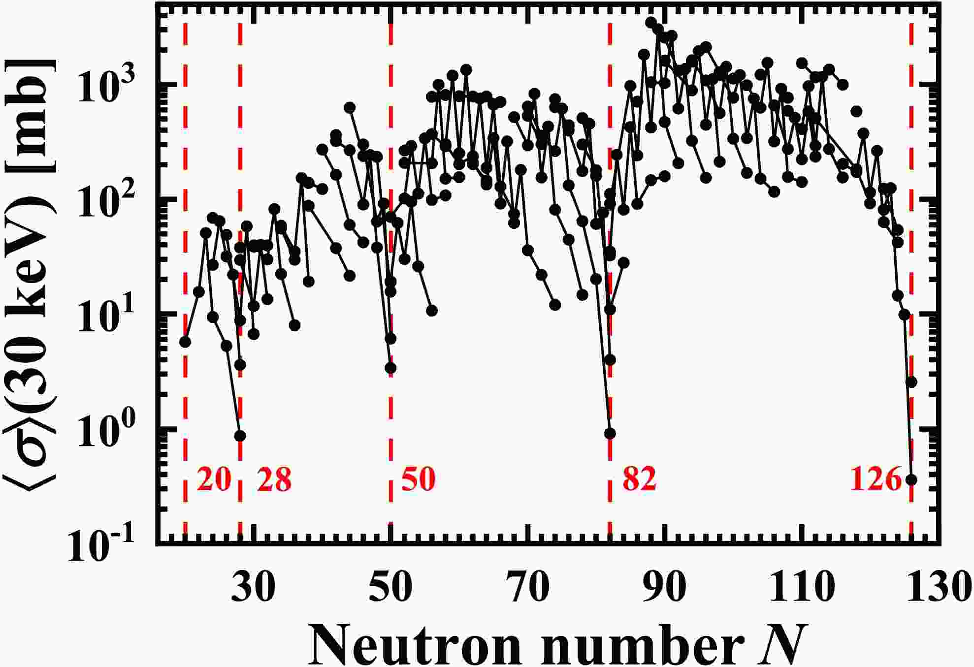
$ (Z, N) $ parities, a pairing effect-related variable$ \delta=1, 2, 3 $ is introduced to classify the even Z-odd N, odd Z-even N, and even Z-even N nuclei. Because there are only three experimental MACS data points of the odd Z-odd N nuclei, they are not included in our study. The experimental MACS results from the Karlsruhe Astrophysical Database of Nucleosynthesis in Stars (KADoNiS) [82] as a function of neutron number N are shown in Fig. 1. It is clear that the MACS of nuclei near the neutron magic numbers in an isotopic chain are significantly smaller than those of their neighboring nuclei. This indicates that shell effects play important roles in describing nuclear MACS [83, 84]; therefore, the shell effect-related variables$ \nu_{n} $ and$ \nu_{p} $ defined in Ref. [48] are also introduced into the input layer of the neural network. As in Refs. [57, 67], we also found that the inclusion of theoretical MACS, which are taken from TENDL-astro 2023, to the input layer can help further improve the prediction accuracy of the neural network [24]. To show the effects of different input features, the BNN approaches with different inputs$ {{\boldsymbol{x}}} = (Z, N) $ ,$ {{\boldsymbol{x}}} = (Z, N, \delta) $ ,$ {{\boldsymbol{x}}} = (Z, N, \delta, \ln\langle\sigma\rangle^{{\rm{th}}}) $ , and$ {{\boldsymbol{x}}} = (Z, N, \delta, \ln\langle\sigma\rangle^{{\rm{th}}}, \nu_n, \nu_p) $ are used for comparison, denoted by BNN-I2, BNN-I3, BNN-I4, and BNN-I6, respectively. The output of the neural network is$ Q^* $ . The numbers of neurons in the hidden layers of the BNN-I2, BNN-I3, BNN-I4, and BNN-I6 approaches are 30, 24, 20, and 15, respectively, which ensures that all of these neural networks have 121 parameters.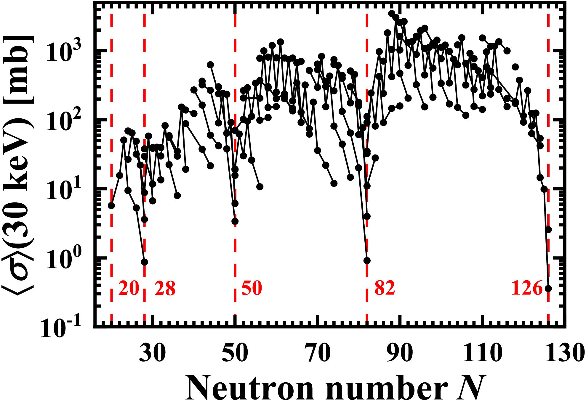
Figure 1. (color online) Experimental MACS from KADoNiS as a function of neutron number N at
$ kT $ = 30 keV. The MACS in each isotopic chain are connected by the solid line.As in Ref. [48], the mathematical expectation and standard deviation of the neural network output over the posterior distribution are used as the MACS predictions and their uncertainties, respectively. In this work, the experimental MACS data at
$ kT = 30 $ keV are taken from KADoNiS [82], while only 238 nuclei with$ Z\geqslant 20 $ remain. The$ S_{2n} $ is taken from the Weizsäcker-Skyrme mass model (WS4) [85], and the parameters$ p_{0}= 0.0159 $ ,$ p_{1}=0.7284 $ are obtained by fitting to the natural logarithm of experimental MACS data from KADoNiS. An exact$ Q^*_{{\rm{ex}}} $ is can then be obtained by using the formula$ Q^*_{{\rm{ex}}}(Z,N)= [\ln\langle\sigma\rangle^{\exp}(Z,N)-\ln p_0]/p_1 $ for each nucleus, which are used as the training data of the BNN approaches. To check the generalization ability of the BNN approach, all$ Q^*_{{\rm{ex}}} $ are separated into two different sets: learning set and testing set. The learning set is built by randomly selecting 80% of nuclei from the total set, and the remaining 20% nuclei compose the testing set. The MACS can then be calculated with the BNN predictions$ Q_{{\rm{BNN}}}^* $ and empirical formula.Because the MACS vary by several orders of magnitude, the root-mean-square (rms) deviation of the natural logarithm of MACS is employed to evaluate the model accuracy:
$ \sigma_{{\rm{rms}}}({\rm{MACS}}) = \sqrt{\sum\limits_{i=1}^n [\ln(\langle\sigma\rangle_i^{\exp} /\langle\sigma\rangle_i^{{\rm{th}}})]^2 /n}, $
(3) where
$ \langle\sigma\rangle_i^{\exp} $ and$ \langle\sigma\rangle_i^{{\rm{th}}} $ are the MACS from KADoNiS and theoretical predictions for nucleus i, respectively, and n is the number of data points to be evaluated. -
Based on the correlation between the two neutron separation energies
$ S_{2n} $ and MACS of neutron-capture reactions$ \langle\sigma\rangle $ , an empirical formula for the MACS was recently proposed [36]:$ \left\langle\sigma\right\rangle( Z,N)=p_0\mathrm{e}^{p_1[S_{2n}(Z,N^*)+p_2]}. $
(1) As in Ref. [36],
$ S_{2n} $ is used instead of$ S_n $ to avoid issues associated with varying spins and parities of the intermediate odd-N nucleus. For the capture on even-N and odd-N nuclei, they use$ S_{2n}(Z,N+2) $ and$ S_{2n}(Z,N+1) $ , respectively. The fixed parameters$ p_{0,1} $ are obtained by fitting to the experimental MACS data. However, the parameter$ p_2 $ cannot be well constrained by the experimental MACS data; therefore, it takes different values in different nuclear regions to improve the accuracy of this empirical formula [36]. Because the role of the parameter$ p_2 $ is to shift the effective$ S_{2n}(Z,N^*) $ , it is possible to combine$ S_{2n}(Z,N^*) $ and$ p_2 $ to obtain a new physical quantity$ Q^*(Z,N)=S_{2n}(Z,N^*)+p_2 $ . This new physical quantity$ Q^* $ contains many neglected and unknown physics in this empirical formula, which can be effectively simulated with the ML method to further improve the predictive ability of this empirical formula.In this study, the BNN approach is employed to describe
$ Q^* $ and can thus calculate the MACS when combined with the empirical formula. In the BNN approach [48, 50], the Bayesian approach is used to analyze the parameters$ {{\boldsymbol{\omega}}} $ of neural networks. Given the dataset$ D =\{({{\boldsymbol{x}}}_{1}, t_1), ({{\boldsymbol{x}}}_{2}, t_2),..., ({{\boldsymbol{x}}}_N, t_N)\} $ , the posterior distribution$ p({{\boldsymbol{\omega}}}|D) $ of parameters$ {{\boldsymbol{\omega}}} $ can be calculated by the Bayes' theorem:$ p({{\boldsymbol{\omega}}}|D) = \frac{p(D|{{\boldsymbol{\omega}}})p({{\boldsymbol{\omega}}})}{p(D)}\propto{p(D|{{\boldsymbol{\omega}}})}, $
(2) where
$ {{\boldsymbol{x}}}_k $ and$ t_k $ ($ k = 1, 2,..., N $ ) are the input and output of the data, respectively; N is the number of data points;$ p({{\boldsymbol{\omega}}}) $ is the prior distribution of parameters$ {{\boldsymbol{\omega}}} $ ; the conditional probability$ p(D|{{\boldsymbol{\omega}}}) $ describes the influence of the data D on$ p({{\boldsymbol{\omega}}}) $ ; and$ p(D) $ is a normalization constant.It has been found that the predictive performance of the neural network can be significantly improved by including more related physical features in its input layer [48, 62, 67]. Due to the remarkable differences in MACS for nuclei with different
$ (Z, N) $ parities, a pairing effect-related variable$ \delta=1, 2, 3 $ is introduced to classify the even Z-odd N, odd Z-even N, and even Z-even N nuclei. Because there are only three experimental MACS data points of the odd Z-odd N nuclei, they are not included in our study. The experimental MACS results from the Karlsruhe Astrophysical Database of Nucleosynthesis in Stars (KADoNiS) [82] as a function of neutron number N are shown in Fig. 1. It is clear that the MACS of nuclei near the neutron magic numbers in an isotopic chain are significantly smaller than those of their neighboring nuclei. This indicates that shell effects play important roles in describing nuclear MACS [83, 84]; therefore, the shell effect-related variables$ \nu_{n} $ and$ \nu_{p} $ defined in Ref. [48] are also introduced into the input layer of the neural network. As in Refs. [57, 67], we also found that the inclusion of theoretical MACS, which are taken from TENDL-astro 2023, to the input layer can help further improve the prediction accuracy of the neural network [24]. To show the effects of different input features, the BNN approaches with different inputs$ {{\boldsymbol{x}}} = (Z, N) $ ,$ {{\boldsymbol{x}}} = (Z, N, \delta) $ ,$ {{\boldsymbol{x}}} = (Z, N, \delta, \ln\langle\sigma\rangle^{{\rm{th}}}) $ , and$ {{\boldsymbol{x}}} = (Z, N, \delta, \ln\langle\sigma\rangle^{{\rm{th}}}, \nu_n, \nu_p) $ are used for comparison, denoted by BNN-I2, BNN-I3, BNN-I4, and BNN-I6, respectively. The output of the neural network is$ Q^* $ . The numbers of neurons in the hidden layers of the BNN-I2, BNN-I3, BNN-I4, and BNN-I6 approaches are 30, 24, 20, and 15, respectively, which ensures that all of these neural networks have 121 parameters.
Figure 1. (color online) Experimental MACS from KADoNiS as a function of neutron number N at
$ kT $ = 30 keV. The MACS in each isotopic chain are connected by the solid line.As in Ref. [48], the mathematical expectation and standard deviation of the neural network output over the posterior distribution are used as the MACS predictions and their uncertainties, respectively. In this work, the experimental MACS data at
$ kT = 30 $ keV are taken from KADoNiS [82], while only 238 nuclei with$ Z\geqslant 20 $ remain. The$ S_{2n} $ is taken from the Weizsäcker-Skyrme mass model (WS4) [85], and the parameters$ p_{0}= 0.0159 $ ,$ p_{1}=0.7284 $ are obtained by fitting to the natural logarithm of experimental MACS data from KADoNiS. An exact$ Q^*_{{\rm{ex}}} $ is can then be obtained by using the formula$ Q^*_{{\rm{ex}}}(Z,N)= [\ln\langle\sigma\rangle^{\exp}(Z,N)-\ln p_0]/p_1 $ for each nucleus, which are used as the training data of the BNN approaches. To check the generalization ability of the BNN approach, all$ Q^*_{{\rm{ex}}} $ are separated into two different sets: learning set and testing set. The learning set is built by randomly selecting 80% of nuclei from the total set, and the remaining 20% nuclei compose the testing set. The MACS can then be calculated with the BNN predictions$ Q_{{\rm{BNN}}}^* $ and empirical formula.Because the MACS vary by several orders of magnitude, the root-mean-square (rms) deviation of the natural logarithm of MACS is employed to evaluate the model accuracy:
$ \sigma_{{\rm{rms}}}({\rm{MACS}}) = \sqrt{\sum\limits_{i=1}^n [\ln(\langle\sigma\rangle_i^{\exp} /\langle\sigma\rangle_i^{{\rm{th}}})]^2 /n}, $
(3) where
$ \langle\sigma\rangle_i^{\exp} $ and$ \langle\sigma\rangle_i^{{\rm{th}}} $ are the MACS from KADoNiS and theoretical predictions for nucleus i, respectively, and n is the number of data points to be evaluated. -
Figure 2(a) shows the
$ Q^*_{{\rm{ex}}} $ obtained using the experimental MACS data from KADoNiS. The$ Q^*_{{\rm{ex}}} $ values are generally approximately 10 MeV, with the smallest value of 4.3 MeV for 208Pb and largest value of 16.9 MeV for 151Eu.$ Q^*_{{\rm{ex}}} $ is generally smaller for the nuclei around magic numbers, resulting in smaller$ \langle\sigma\rangle $ , as shown in Fig. 1. The odd-even staggering is also found for$ Q^*_{{\rm{ex}}} $ , which means that$ Q^*_{{\rm{ex}}} $ appears with smaller and larger values alternately. Taking the Sm ($ Z=62 $ ) isotopes as an example, it is clear that the$ Q^*_{{\rm{ex}}} $ values for the odd-N nuclei are generally larger than those for the neighboring even-N nuclei. The BNN approach is used to describe$ Q^*_{{\rm{ex}}} $ , and the differences between the BNN-I6 predictions$ Q^*_{{\rm{BNN}}} $ and$ Q^*_{{\rm{ex}}} $ are shown in Fig. 2(b). Clearly, BNN-I6 well-reproduces the$ Q^*_{{\rm{ex}}} $ values with their differences being less than 0.7 MeV.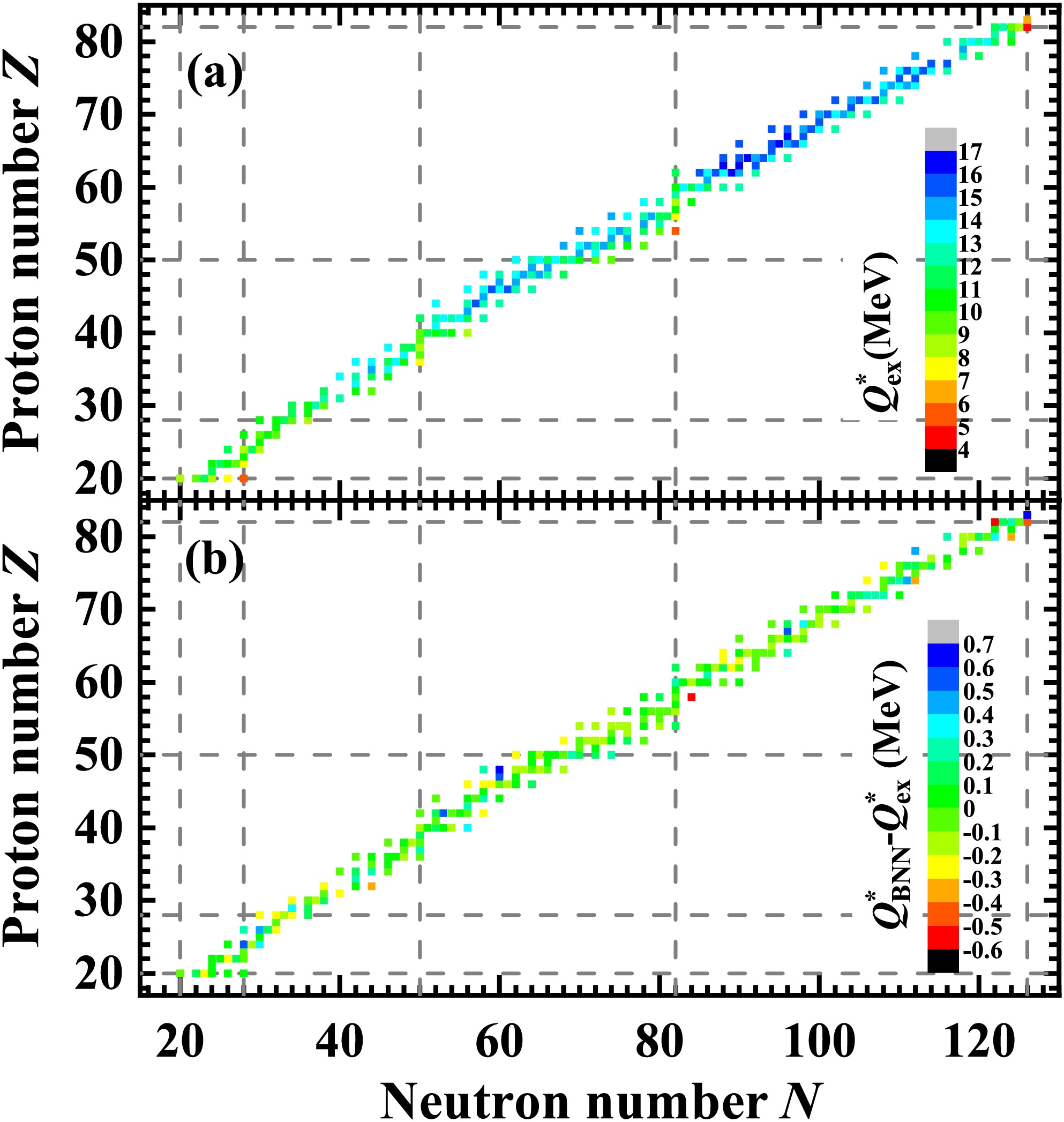
Figure 2. (color online) (a)
$ Q^*_{{\rm{ex}}} $ obtained with the experimental MACS data from KADoNiS. (b) Differences between the BNN-I6 predictions$ Q^*_{{\rm{BNN}}} $ and$ Q^*_{{\rm{ex}}} $ . The dashed lines denote the traditional magic numbers.With the BNN-I6 predictions of
$ Q^*_{{\rm{BNN}}} $ , the parameters$ p_0 $ and$ p_1 $ can be further updated by fitting them to the experimental MACS data. Using these updated parameters$ p_0 $ and$ p_1 $ , we can calculate the new exact$ Q_{{\rm{ex}}}^* $ values, train the BNN with them, and make predictions with the new$ Q_{{\rm{BNN}}}^* $ values and empirical formula. We have performed five iterations using the same procedure, and the results are summarized in Tabel 1. The differences in the rms deviations$ \sigma_{{\rm{rms}}}({\rm{MACS}}) $ of the first five iterations are only 0.0060, 0.0148, and 0.0081 for the learning, testing, and total sets, respectively. This indicates that the iteration between the empirical formula and BNN-I6 approach has a limited impact on the MACS predictions. The MACS predictions from the first iteration are used as the final predictions in this study, as they are the most accurate.Round $ p_0 $ $ p_1 $ Learning set Testing set Total set 1st 0.0159 0.7284 0.1308 0.1603 0.1373 2nd 0.0156 0.7295 0.1331 0.1728 0.1420 3th 0.0155 0.7308 0.1328 0.1661 0.1402 4th 0.0152 0.7317 0.1310 0.1635 0.1381 5th 0.0150 0.7330 0.1368 0.1751 0.1453 Table 1. Parameters
$ p_0 $ and$ p_1 $ for the first five iterations between the empirical formula and BNN-I6 approach, along with the rms deviations$ \sigma_{{\rm{rms}}}({\rm{MACS}}) $ with respect to the experimental MACS data for the learning, testing, and total sets.Figure 3 shows the rms deviations
$ \sigma_{{\rm{rms}}}({\rm{MACS}}) $ of different BNN predictions with respect to the experimental MACS data from KADoNiS for the learning, testing, and total sets. Clearly, the predictive performance of the BNN approach is gradually improved by including an increasing number of related physical inputs, i.e., δ,$ \ln\langle\sigma\rangle^{{\rm{th}}} $ ,$ \nu_n $ , and$ \nu_p $ . By comparing BNN-I2 and BNN-I3, it is clear that the rms deviations are significantly reduced by including δ not only for the learning set but also for the testing and total sets. The inclusion of the theoretical MACS$ \ln\langle\sigma\rangle^{{\rm{th}}} $ further reduces the rms deviations. BNN-I4 achieves an rms of 0.2443 on the testing set, which is even smaller than the value of 0.2545 for TENDL-astro 2023. By further including$ \nu_{n} $ and$ \nu_{p} $ , BNN-I6 achieves the best predictive performance, with rms deviations of 0.1308, 0.1603, and 0.1373 for the learning, testing, and total sets, respectively. In addition, the kernel ridge regression (KRR) approach has been employed to improve the prediction accuracy by learning the logarithmic residuals between the theoretical and experimental MACS at different temperatures in Ref. [68]. This study optimizes the KRR hyperparameters by employing leave-one-nucleus-out cross validation (LONOCV) and leave-one-data-out cross validation (LODOCV), successfully predicting the MACS at different temperatures. The rms of BNN-I6 in the present study is larger than that of KRR-LODOCV but smaller than that of KRR-LONOCV.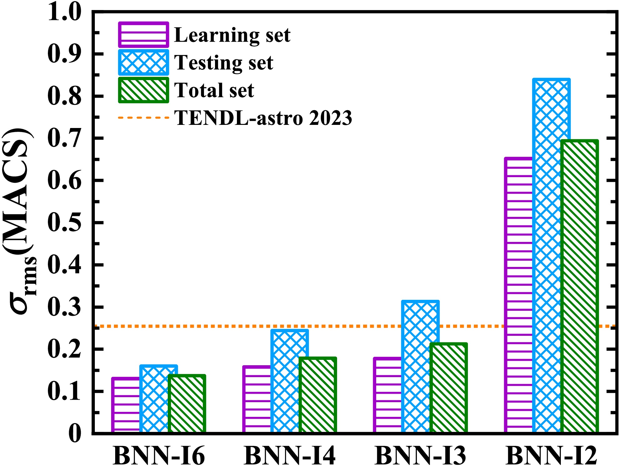
Figure 3. (color online) Rms deviations
$ \sigma_{{\rm{rms}}}({\rm{MACS}}) $ of different BNN predictions with respect to the experimental MACS data from KADoNiS for learning, testing, and total sets. The corresponding rms deviation of TENDL-astro 2023 for the total set is shown by the dashed line for comparison.Taking Pb isotopes and
$ N=50 $ isotones as examples, the MACS predicted by the BNN-I6 and BNN-I3 approaches are shown in Fig. 4. Both the BNN and TENDL-astro 2023 well describe the phenomena of the abrupt decrease at neutron magic number and the odd–even staggering in the experimental MACS data, while BNN-I6 reproduces the experimental MACS data better than BNN-I3 and TENDL-astro 2023. When extrapolating to the region without the experimental MACS data, the uncertainties of the BNN predictions gradually increase. For the Pb isotopes, BNN-I6 predicts an increasing trend after$ N=126 $ , as does TENDL-astro 2023, but BNN-I3 predicts a different decreasing trend and larger MACS uncertainties. This implies that the shell effects in the MACS data can be better extracted by the BNN approach by including the input features$ \ln\langle\sigma\rangle^{{\rm{th}}} $ ,$ \nu_n $ , and$ \nu_p $ . We also perform calculations using the BNN with inputs$ {{\boldsymbol{x}}} = (Z, N, \delta, \ln\langle\sigma\rangle^{{\rm{th}}}) $ or$ {{\boldsymbol{x}}} = (Z, N, \delta, \nu_n, \nu_p) $ . The results also predict an increasing trend after$ N=126 $ , which indicates that the inclusion of$ \ln\langle\sigma\rangle^{{\rm{th}}} $ or ($ \nu_n, \nu_p $ ) can help extract the shell effects in the MACS data, while the quantitative description can be further improved if$ \ln\langle\sigma\rangle^{{\rm{th}}} $ and$ \nu_n, \nu_p $ are all included. For the$ N=50 $ isotones, TENDL-astro 2023 predicts larger MACS for 86Kr and 87Rb, while BNN-I6 well reproduces the experimental MACS and also predicts smaller MACS than TENDL-astro 2023 for the$ N=50 $ isotones with smaller proton numbers. The theoretical description of MACS for magic nuclei is relatively challenging; the rms deviation$ \sigma_{{\rm{rms}}}({\rm{MACS}}) $ of TENDL-astro 2023 is 0.4182 for magic nuclei, while it is only 0.1994 for other nuclei. The BNN-I6 approach significantly improves the description of MACS with rms deviations of 0.1630 for magic nuclei and 0.1306 for other nuclei.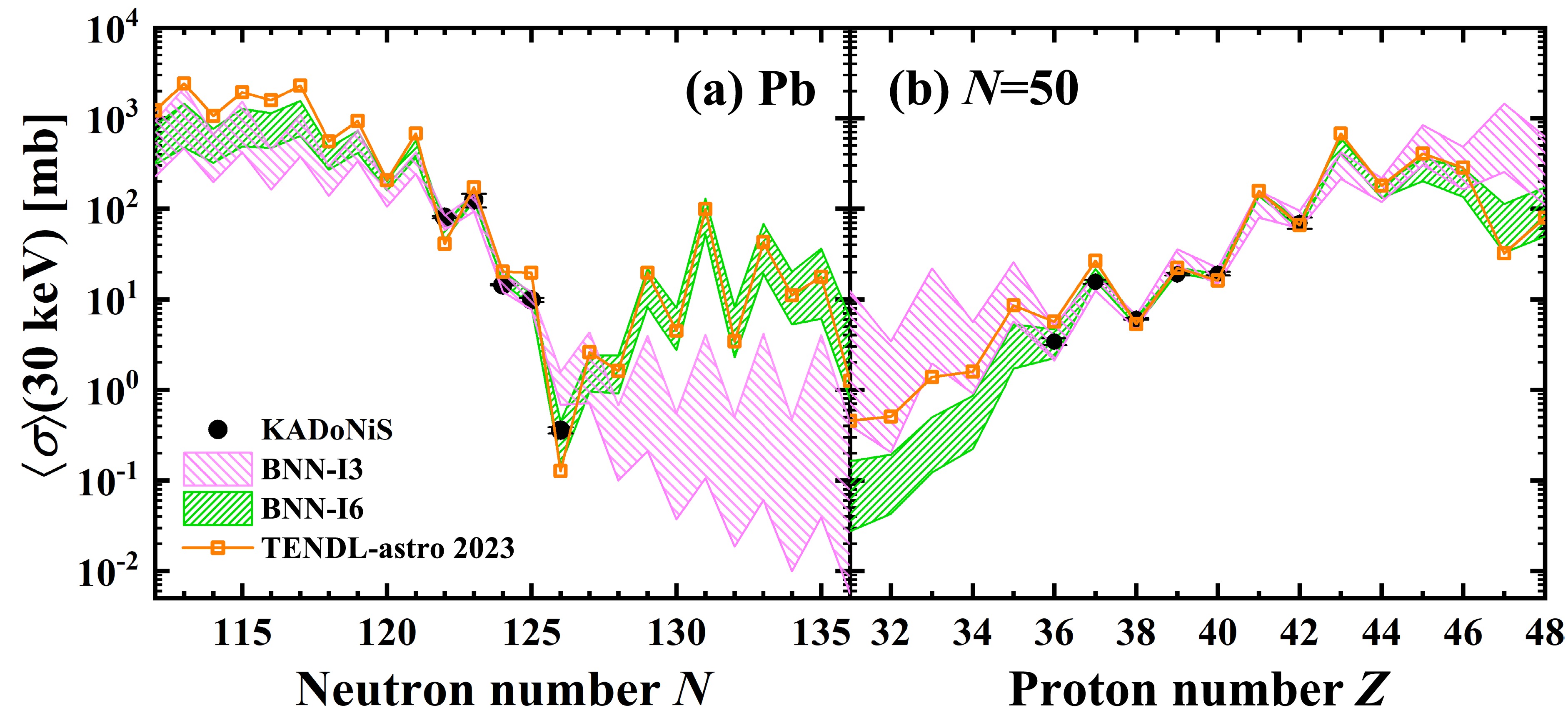
Figure 4. (color online) MACS of Pb isotopes (a) and
$ N=50 $ isotones (b) at$ kT = 30 $ keV. The BNN-I6 and BNN-I3 predictions with their uncertainties are represented by slash hatched regions and backslash hatched regions, respectively. For comparison, the experimental MACS data from KADoNiS and MACS predictions from TENDL-astro 2023 are shown by filled circles and open squares, respectively.To further study the performance of the BNN-I6 approach, the MACS predicted by the BNN-I6 approach are compared with the experimental data and results from the empirical formula in Ref. [36] (Formula Couture) and TENDL-astro 2023, which are shown in Fig. 5 by taking Xe and Sm isotopes and
$ N=96 $ isotones as examples. As the$ \ln\langle\sigma\rangle^{{\rm{th}}} $ value from TENDL-astro 2023 is one of the inputs of the BNN-I6 approach, the predicted MACS by BNN-I6 are generally consistent with the trend of the TENDL-astro 2023 results. However, the predictive performance of the BNN-I6 approach is much better than that of TENDL-astro 2023 for magic nuclei, such as 136Xe. Compared with the Formula Couture, BNN-I6 can not only reproduce the experimental MACS more accurately but also be applied to predict the MACS of more neutron-rich nuclei far from the β-stability line. This indicates that the method of combining machine learning with a physics-driven empirical formula can effectively improve the predictive accuracy of nuclear properties while ensuring the robustness and interpretability of the model.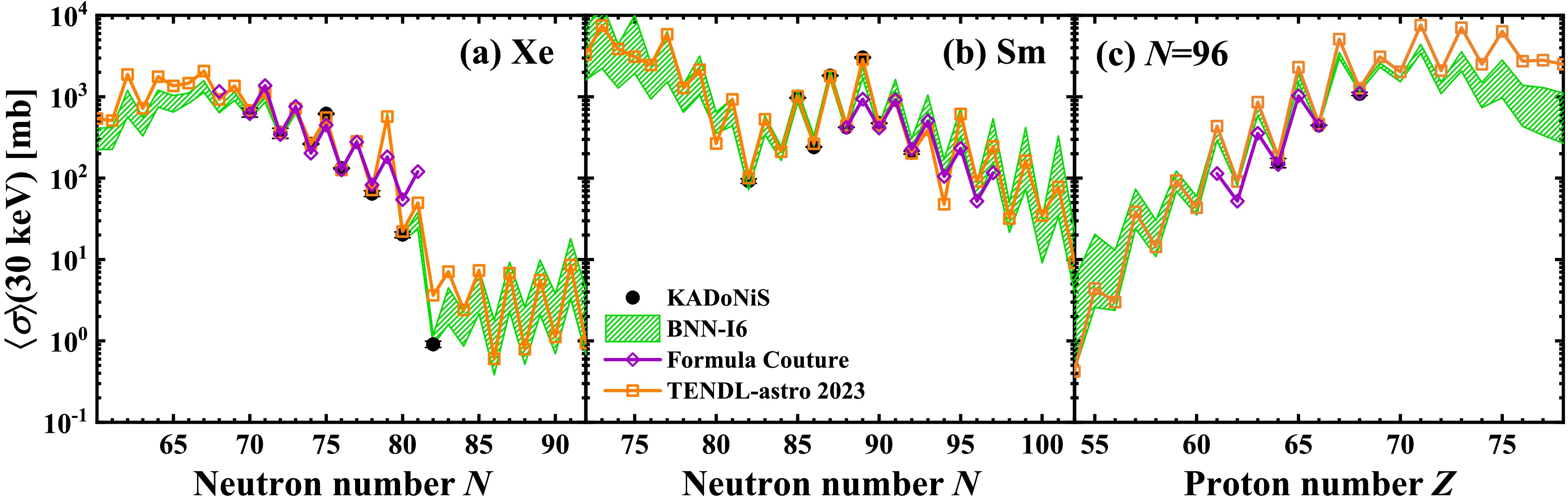
Figure 5. (color online) MACS of Xe isotopes (a), Sm isotopes (b), and
$ N=96 $ isotones (c) at$ kT = 30 $ keV. The BNN-I6 predictions with their uncertainties are represented by slash hatched regions. For comparison, the experimental MACS data from KADoNiS and the MACS predictions from TENDL-astro 2023 and the empirical formula in Ref. [36] are shown by filled circles, open squares, and open diamonds, respectively.The MACS predicted by the BNN-I6 approach are shown in Fig. 6. The predicted MACS generally decrease for the nuclei with a smaller proton number and larger neutron number. Moreover, the MACS of nuclei with odd neutron numbers are generally larger than those of neighboring isotopes with even neutron numbers, which induces the clear odd-even staggering observed in Fig. 6. It is also clear that the MACS of the nuclei near the neutron magic numbers are generally smaller than those of neighboring nuclei, particularly around doubly magic nuclei, such as 78Ni and 132Sn.
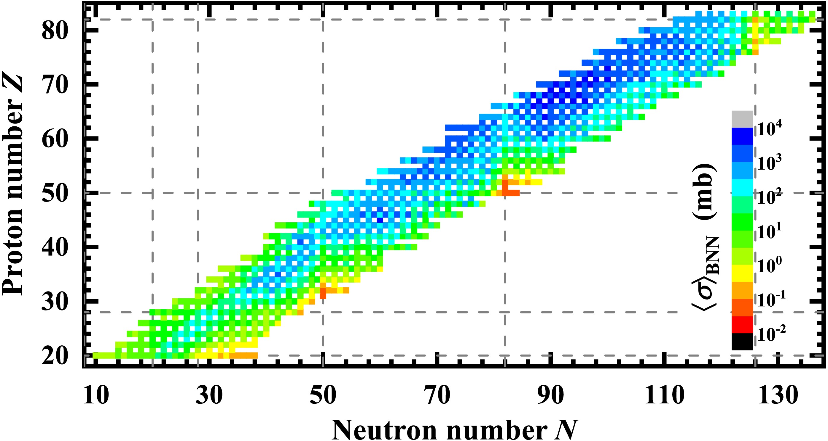
Figure 6. (color online) MACS predicted by BNN-I6 at
$ kT $ = 30 keV. -
Figure 2(a) shows the
$ Q^*_{{\rm{ex}}} $ obtained using the experimental MACS data from KADoNiS. The$ Q^*_{{\rm{ex}}} $ values are generally approximately 10 MeV, with the smallest value of 4.3 MeV for 208Pb and largest value of 16.9 MeV for 151Eu.$ Q^*_{{\rm{ex}}} $ is generally smaller for the nuclei around magic numbers, resulting in smaller$ \langle\sigma\rangle $ , as shown in Fig. 1. The odd-even staggering is also found for$ Q^*_{{\rm{ex}}} $ , which means that$ Q^*_{{\rm{ex}}} $ appears with smaller and larger values alternately. Taking the Sm ($ Z=62 $ ) isotopes as an example, it is clear that the$ Q^*_{{\rm{ex}}} $ values for the odd-N nuclei are generally larger than those for the neighboring even-N nuclei. The BNN approach is used to describe$ Q^*_{{\rm{ex}}} $ , and the differences between the BNN-I6 predictions$ Q^*_{{\rm{BNN}}} $ and$ Q^*_{{\rm{ex}}} $ are shown in Fig. 2(b). Clearly, BNN-I6 well-reproduces the$ Q^*_{{\rm{ex}}} $ values with their differences being less than 0.7 MeV.
Figure 2. (color online) (a)
$ Q^*_{{\rm{ex}}} $ obtained with the experimental MACS data from KADoNiS. (b) Differences between the BNN-I6 predictions$ Q^*_{{\rm{BNN}}} $ and$ Q^*_{{\rm{ex}}} $ . The dashed lines denote the traditional magic numbers.With the BNN-I6 predictions of
$ Q^*_{{\rm{BNN}}} $ , the parameters$ p_0 $ and$ p_1 $ can be further updated by fitting them to the experimental MACS data. Using these updated parameters$ p_0 $ and$ p_1 $ , we can calculate the new exact$ Q_{{\rm{ex}}}^* $ values, train the BNN with them, and make predictions with the new$ Q_{{\rm{BNN}}}^* $ values and empirical formula. We have performed five iterations using the same procedure, and the results are summarized in Tabel 1. The differences in the rms deviations$ \sigma_{{\rm{rms}}}({\rm{MACS}}) $ of the first five iterations are only 0.0060, 0.0148, and 0.0081 for the learning, testing, and total sets, respectively. This indicates that the iteration between the empirical formula and BNN-I6 approach has a limited impact on the MACS predictions. The MACS predictions from the first iteration are used as the final predictions in this study, as they are the most accurate.Round $ p_0 $ $ p_1 $ Learning set Testing set Total set 1st 0.0159 0.7284 0.1308 0.1603 0.1373 2nd 0.0156 0.7295 0.1331 0.1728 0.1420 3th 0.0155 0.7308 0.1328 0.1661 0.1402 4th 0.0152 0.7317 0.1310 0.1635 0.1381 5th 0.0150 0.7330 0.1368 0.1751 0.1453 Table 1. Parameters
$ p_0 $ and$ p_1 $ for the first five iterations between the empirical formula and BNN-I6 approach, along with the rms deviations$ \sigma_{{\rm{rms}}}({\rm{MACS}}) $ with respect to the experimental MACS data for the learning, testing, and total sets.Figure 3 shows the rms deviations
$ \sigma_{{\rm{rms}}}({\rm{MACS}}) $ of different BNN predictions with respect to the experimental MACS data from KADoNiS for the learning, testing, and total sets. Clearly, the predictive performance of the BNN approach is gradually improved by including an increasing number of related physical inputs, i.e., δ,$ \ln\langle\sigma\rangle^{{\rm{th}}} $ ,$ \nu_n $ , and$ \nu_p $ . By comparing BNN-I2 and BNN-I3, it is clear that the rms deviations are significantly reduced by including δ not only for the learning set but also for the testing and total sets. The inclusion of the theoretical MACS$ \ln\langle\sigma\rangle^{{\rm{th}}} $ further reduces the rms deviations. BNN-I4 achieves an rms of 0.2443 on the testing set, which is even smaller than the value of 0.2545 for TENDL-astro 2023. By further including$ \nu_{n} $ and$ \nu_{p} $ , BNN-I6 achieves the best predictive performance, with rms deviations of 0.1308, 0.1603, and 0.1373 for the learning, testing, and total sets, respectively. In addition, the kernel ridge regression (KRR) approach has been employed to improve the prediction accuracy by learning the logarithmic residuals between the theoretical and experimental MACS at different temperatures in Ref. [68]. This study optimizes the KRR hyperparameters by employing leave-one-nucleus-out cross validation (LONOCV) and leave-one-data-out cross validation (LODOCV), successfully predicting the MACS at different temperatures. The rms of BNN-I6 in the present study is larger than that of KRR-LODOCV but smaller than that of KRR-LONOCV.
Figure 3. (color online) Rms deviations
$ \sigma_{{\rm{rms}}}({\rm{MACS}}) $ of different BNN predictions with respect to the experimental MACS data from KADoNiS for learning, testing, and total sets. The corresponding rms deviation of TENDL-astro 2023 for the total set is shown by the dashed line for comparison.Taking Pb isotopes and
$ N=50 $ isotones as examples, the MACS predicted by the BNN-I6 and BNN-I3 approaches are shown in Fig. 4. Both the BNN and TENDL-astro 2023 well describe the phenomena of the abrupt decrease at neutron magic number and the odd–even staggering in the experimental MACS data, while BNN-I6 reproduces the experimental MACS data better than BNN-I3 and TENDL-astro 2023. When extrapolating to the region without the experimental MACS data, the uncertainties of the BNN predictions gradually increase. For the Pb isotopes, BNN-I6 predicts an increasing trend after$ N=126 $ , as does TENDL-astro 2023, but BNN-I3 predicts a different decreasing trend and larger MACS uncertainties. This implies that the shell effects in the MACS data can be better extracted by the BNN approach by including the input features$ \ln\langle\sigma\rangle^{{\rm{th}}} $ ,$ \nu_n $ , and$ \nu_p $ . We also perform calculations using the BNN with inputs$ {{\boldsymbol{x}}} = (Z, N, \delta, \ln\langle\sigma\rangle^{{\rm{th}}}) $ or$ {{\boldsymbol{x}}} = (Z, N, \delta, \nu_n, \nu_p) $ . The results also predict an increasing trend after$ N=126 $ , which indicates that the inclusion of$ \ln\langle\sigma\rangle^{{\rm{th}}} $ or ($ \nu_n, \nu_p $ ) can help extract the shell effects in the MACS data, while the quantitative description can be further improved if$ \ln\langle\sigma\rangle^{{\rm{th}}} $ and$ \nu_n, \nu_p $ are all included. For the$ N=50 $ isotones, TENDL-astro 2023 predicts larger MACS for 86Kr and 87Rb, while BNN-I6 well reproduces the experimental MACS and also predicts smaller MACS than TENDL-astro 2023 for the$ N=50 $ isotones with smaller proton numbers. The theoretical description of MACS for magic nuclei is relatively challenging; the rms deviation$ \sigma_{{\rm{rms}}}({\rm{MACS}}) $ of TENDL-astro 2023 is 0.4182 for magic nuclei, while it is only 0.1994 for other nuclei. The BNN-I6 approach significantly improves the description of MACS with rms deviations of 0.1630 for magic nuclei and 0.1306 for other nuclei.
Figure 4. (color online) MACS of Pb isotopes (a) and
$ N=50 $ isotones (b) at$ kT = 30 $ keV. The BNN-I6 and BNN-I3 predictions with their uncertainties are represented by slash hatched regions and backslash hatched regions, respectively. For comparison, the experimental MACS data from KADoNiS and MACS predictions from TENDL-astro 2023 are shown by filled circles and open squares, respectively.To further study the performance of the BNN-I6 approach, the MACS predicted by the BNN-I6 approach are compared with the experimental data and results from the empirical formula in Ref. [36] (Formula Couture) and TENDL-astro 2023, which are shown in Fig. 5 by taking Xe and Sm isotopes and
$ N=96 $ isotones as examples. As the$ \ln\langle\sigma\rangle^{{\rm{th}}} $ value from TENDL-astro 2023 is one of the inputs of the BNN-I6 approach, the predicted MACS by BNN-I6 are generally consistent with the trend of the TENDL-astro 2023 results. However, the predictive performance of the BNN-I6 approach is much better than that of TENDL-astro 2023 for magic nuclei, such as 136Xe. Compared with the Formula Couture, BNN-I6 can not only reproduce the experimental MACS more accurately but also be applied to predict the MACS of more neutron-rich nuclei far from the β-stability line. This indicates that the method of combining machine learning with a physics-driven empirical formula can effectively improve the predictive accuracy of nuclear properties while ensuring the robustness and interpretability of the model.
Figure 5. (color online) MACS of Xe isotopes (a), Sm isotopes (b), and
$ N=96 $ isotones (c) at$ kT = 30 $ keV. The BNN-I6 predictions with their uncertainties are represented by slash hatched regions. For comparison, the experimental MACS data from KADoNiS and the MACS predictions from TENDL-astro 2023 and the empirical formula in Ref. [36] are shown by filled circles, open squares, and open diamonds, respectively.The MACS predicted by the BNN-I6 approach are shown in Fig. 6. The predicted MACS generally decrease for the nuclei with a smaller proton number and larger neutron number. Moreover, the MACS of nuclei with odd neutron numbers are generally larger than those of neighboring isotopes with even neutron numbers, which induces the clear odd-even staggering observed in Fig. 6. It is also clear that the MACS of the nuclei near the neutron magic numbers are generally smaller than those of neighboring nuclei, particularly around doubly magic nuclei, such as 78Ni and 132Sn.
Figure 6. (color online) MACS predicted by BNN-I6 at
$ kT $ = 30 keV. -
In summary, the MACS of the neutron-capture reaction at 30 keV are studied with the BNN approach in combination with a recently proposed empirical formula for the cross sections. The BNN is employed to describe a physical quantity
$ Q^* $ related to the reaction energy, and then, the MACS can be calculated with the BNN predictions$ Q_{{\rm{BNN}}}^* $ combined with the empirical formula. In addition to the proton and neutron numbers, four physical quantities are found to be important for improving the predictive performance of the BNN approach: the pairing effect-related variable δ, shell effect-related variables$ \nu_{n} $ and$ \nu_{p} $ , and theoretical neutron-capture reaction cross sections. The BNN approach achieves a more accurate description of the experimental MACS data from KADoNiS compared with the TENDL-astro 2023 theoretical library calculated using the TALYS code based on the Hauser–Feshbach statistical model, especially the MACS data of magic nuclei. The rms deviation of the BNN approach with respect to the natural logarithm of the experimental MACS data is reduced to 0.1373, which is much smaller than the value of 0.2545 for TENDL-astro 2023. Compared with the Formula Couture, the BNN can not only reproduce the experimental MACS more accurately but also be applied to predict the MACS of more neutron-rich nuclei far from the β-stability line. When extrapolated to the unknown region, the BNN predictions align well with MACS trends predicted by TENDL-astro 2023, though there are quantitative deviations between them. Therefore, the method of combining machine learning with a physics-driven empirical formula can effectively improve the predictive accuracy of nuclear properties while ensuring the robustness and interpretability of the model, which can also be used to study other nuclear properties, such as nuclear masses and half-lives. -
In summary, the MACS of the neutron-capture reaction at 30 keV are studied with the BNN approach in combination with a recently proposed empirical formula for the cross sections. The BNN is employed to describe a physical quantity
$ Q^* $ related to the reaction energy, and then, the MACS can be calculated with the BNN predictions$ Q_{{\rm{BNN}}}^* $ combined with the empirical formula. In addition to the proton and neutron numbers, four physical quantities are found to be important for improving the predictive performance of the BNN approach: the pairing effect-related variable δ, shell effect-related variables$ \nu_{n} $ and$ \nu_{p} $ , and theoretical neutron-capture reaction cross sections. The BNN approach achieves a more accurate description of the experimental MACS data from KADoNiS compared with the TENDL-astro 2023 theoretical library calculated using the TALYS code based on the Hauser–Feshbach statistical model, especially the MACS data of magic nuclei. The rms deviation of the BNN approach with respect to the natural logarithm of the experimental MACS data is reduced to 0.1373, which is much smaller than the value of 0.2545 for TENDL-astro 2023. Compared with the Formula Couture, the BNN can not only reproduce the experimental MACS more accurately but also be applied to predict the MACS of more neutron-rich nuclei far from the β-stability line. When extrapolated to the unknown region, the BNN predictions align well with MACS trends predicted by TENDL-astro 2023, though there are quantitative deviations between them. Therefore, the method of combining machine learning with a physics-driven empirical formula can effectively improve the predictive accuracy of nuclear properties while ensuring the robustness and interpretability of the model, which can also be used to study other nuclear properties, such as nuclear masses and half-lives.
Predictions of neutron-capture reaction cross sections using a Bayesian neural network approach combined with a physically motivated empirical formula
- Received Date: 2026-01-11
- Available Online: 2026-06-15
Abstract: Neutron-capture reaction cross sections are studied using the Bayesian neural network (BNN) approach in combination with a recently proposed empirical formula for the cross sections. In addition to the proton and neutron numbers, four physical quantities are found to be important for improving the predictive performance of the BNN approach: the pairing effect-related variable δ, shell effect-related variables $ \nu_{n} $ and $ \nu_{p} $, and theoretical neutron-capture reaction cross sections. The BNN approach more effectively describes the Maxwellian-averaged ($ n,\gamma $) cross sections (MACS) at $ kT $ = 30 keV than the TENDL-astro 2023 theoretical library calculated using TALYS code based on the Hauser–Feshbach statistical model. The root-mean-square deviation of the BNN approach with respect to the natural logarithm of the experimental MACS data from the Karlsruhe Astrophysical Database of Nucleosynthesis in Stars is reduced to 0.1373, compared with the value of 0.2545 for TENDL-astro 2023. The BNN predictions align well with MACS trends predicted by TENDL-astro 2023 when extrapolated to the unknown region, though there are quantitative deviations between them.


 DownLoad: