Elucidating the nature of axial-vector charm-antibottom tetraquark states

Although the existence of hadrons with more sophisticated configurations than those comprising $ q\bar{q} $ and $ qqq $ has been known for several decades, the experimental confirmation of the presence of the exotic state labeled X(3872) was accomplished by the Belle Collaboration in 2003 [1]. Subsequently, various experimental collaborations have identified a considerable number of exotic states. With each new observation, the family of such exotic states continues to diversify, representing a dynamically evolving and active field within hadron physics, encompassing experimental and theoretical approaches. Various theoretical explanations have been put forth to elucidate the true nature of these states. These explanations have been proposed in conjunction with several different theoretical constructs, including more traditional hadrons, loosely bound molecular states, compact pentaquarks or tetraquarks, hybrids, glueballs, kinematic effects, and other related concepts. However, despite comprehensive investigations, both theoretical and experimental, the fundamental questions concerning the nature, quantum numbers, and decay properties of these exotic states remain unresolved. A list of the most recent advances in the domain of exotic states can be found in Refs. [2−17].

Most observed tetraquark states are classified as hidden-charm or hidden-bottom tetraquark states, encompassing the $ c \bar{c} $ or $ b \bar{b} $ pair. Nevertheless, the fundamental principles of QCD do not preclude the theoretical possibility of open-flavour tetraquark states. The $ [qc] [\bar{q} \bar{b}] $ with q = u, d, and s tetraquark states represent a distinct category of exotic state. A considerable amount of theoretical information on the expected properties of these tetraquark states is available in the literature since the original studies began more than two decades ago [18−28]. While these specific tetraquark configurations have not yet been observed experimentally, they represent a theoretically compelling subject in hadron spectroscopy. The $ [qc][\bar{q}\bar{b}] $ system is particularly noteworthy because, unlike hidden-flavor tetraquarks (e.g., $ c\bar{c}q\bar{q} $ or $ b\bar{b}q\bar{q} $), it possesses inherent stability and is expected to exhibit narrow decay widths. This distinctive feature arises from the flavor-asymmetric quark content, which forbids annihilation into gluons—a dominant decay channel for many conventional quarkonia and hidden-flavor exotic states [28]. These properties render them a valuable resource for the study of heavy-quark dynamics and a deeper understanding of the dynamics of QCD. To gain a deeper understanding of the internal structures of these states, it is also crucial to investigate the decay channels, including strong, radiative, and electromagnetic, in conjunction with their spectroscopic parameters.

The study of the electromagnetic properties of tetraquark states provides a crucial window into their internal quark-gluon structure and serves as a powerful probe of non-perturbative QCD dynamics. Among these properties, the magnetic dipole moment stands out as a particularly sensitive observable, as it directly reflects the spatial distribution of charges and spins within the hadron. This work aims to determine the magnetic moments of the axial-vector charm-antibottom tetraquark states, denoted as $ [qc][\bar{q}^\prime \bar{b}] $ and $ [qc][\bar{q} \bar{b}] $ (for short $ Z_{\bar{b} c} $) using the framework of QCD light-cone sum rules (LCSR). We construct these states in a compact diquark-antidiquark configuration with spin-parity quantum numbers ${J^P} = 1^{+}$. Recent experimental discoveries have revealed a rich spectrum of exotic hadrons, with many states exhibiting properties consistent with loosely bound molecular configurations of conventional mesons and baryons. While this molecular picture is phenomenologically successful for numerous candidates, it is crucial to recognize that QCD fundamentally permits another distinct class of exotic states: compact tetraquarks, where all four valence quarks are confined within a single, small-volume color-singlet object. The central challenge in contemporary hadron spectroscopy lies not in choosing between these two paradigms but in developing tools to distinguish them unambiguously. In this context, electromagnetic properties, particularly the magnetic dipole moment, emerge as exceptionally sensitive and discriminating probes. Unlike the mass, which can be similar for molecular and compact configurations due to intricate binding dynamics, the magnetic moment is directly governed by the intrinsic spatial distribution of charges and spins within the hadron. A compact diquark-antidiquark system, characterized by strongly correlated quark pairs in a small volume, is expected to produce a magnetic response fundamentally different from that of a loosely bound hadronic molecule, where the constituent mesons largely preserve their individual electromagnetic identities. Therefore, precise theoretical predictions for the magnetic moments of specific tetraquark configurations establish critical theoretical benchmarks against which future experimental measurements can be compared. Consequently, this work is dedicated to providing first-principles predictions for the magnetic moments of the axial-vector $ Z_{\bar{b} c} $ tetraquark states within the compact diquark-antidiquark picture using LCSR. Our calculations yield concrete numerical predictions that serve as a reference for the compact scenario. Should future high-precision experiments at facilities like LHCb, Belle II, or a future electron-positron super factory succeed in measuring the electromagnetic properties of a charged $ Z_{\bar{b} c} $-like resonance, a direct comparison with our results could provide compelling evidence for or against its interpretation as a compact tetraquark. This strategy of utilizing electromagnetic observables to disentangle competing structural models represents a vital and necessary direction for advancing our understanding of exotic hadron structure. This research extends the systematic investigation of electromagnetic properties into the open-charm-bottom tetraquark sector. It builds upon a substantial body of prior work examining the electromagnetic characteristics of both hidden- and doubly-heavy tetraquark states [29−53] and pentaquark states [54−78]. It is evident that further research is required to gain a deeper understanding of the electromagnetic characteristics of states with varying structural compositions.

This paper is organized as follows: Section II is concerned with deriving the LCSR for the magnetic moment of $ Z_{\bar{b} c} $ states with quantum numbers ${J^{P}}= 1^{+}$. Section III is dedicated to the numerical examination of the sum rules derived for these states. In Section IV, possible scenarios for the experimental measurement of the obtained magnetic and quadrupole moments are presented. Finally, Section V presents our concluding remarks.

This section presents the derivation of LCSR for $ Z_{\bar{b} c} $ states. To obtain the relevant sum rules, the following correlation function is considered:

where F denotes the external electromagnetic field, while $ J^i_{\mu(\nu)}(x) $ denotes the interpolating currents, which correspond to the $ Z_{ \bar{b} c} $ tetraquark states.

Under the prescriptions of the LCSR, the analysis processes can be written as follows:

● The correlation function is derived in terms of hadronic parameters, such as mass, residue, and form factors, which is referred to as the "hadronic representation."

● The correlation function is also derived in terms of parameters associated with the QCD parameters, including quark-gluon degrees of freedom and distribution amplitudes, which is referred to as the "QCD representation."

● In the final step, the aforementioned representations are equalized with the help of the quark-hadron duality assumption. To remove any unwanted contributions from the analyses, a double Borel transformation and continuum subtractions are performed to obtain sum rules for the physical parameter to be calculated.

In accordance with the procedure described above, our analysis starts by examining the hadronic formulation of the relevant tetraquark states.

By the prescription outlined above, we may now commence the magnetic moment analyses of $ Z_{\bar{b} c} $ tetraquark states. To obtain the hadronic representation of the correlation function, we plug a complete set of intermediate $ Z_{\bar{b} c} $ tetraquark states with the same quantum numbers as the interpolating currents into the correlation function. Then, taking the integral over x, we get the following results:

In Eq. (2), there are matrix elements whose explicit forms are required as follows [79]:

where $ \lambda_{Z_{\bar{b} c}} $ and $ \varepsilon_\mu^i (\varepsilon_\nu^{*f}) $ are the residue and polarization vector of the initial and final $ Z_{\bar{b} c} $ tetraquark states, respectively; $ \varepsilon^\gamma $ is the polarization vector of the photon, and $ G_i(Q^2) $ are Lorentz invariant form factors of the corresponding radiative transition with $ Q^2=-q^2 $.

Upon substituting Eqs. (3)−(5) into Eq. (2), the hadronic representation of the correlation function of the $ Z_{\bar{b} c} $ tetraquark states takes the following form:

The magnetic form factor, denoted as $ F_M(Q^2) $, can be derived under the established methodology for deriving the aforementioned form factors, $ G_i(Q^2) $, as follows:

In the static limit ($ Q^2=0 $), where the photon is regarded as a real particle, the magnetic moment ($ \mu_{Z_{\bar{b} c}} $) can be characterized as follows:

where $ m_N $ is nucleon mass and $ \mu_N $ represents the nuclear magneton.

The final equation has been obtained, thus enabling the hadronic representation of the analysis to be derived. The second step of the aforementioned prescription may now be initiated, namely, the derivation of the correlation function in terms of QCD parameters.

To compute the magnetic moments of the axial-vector tetraquark states via LCSR, one must first construct appropriate interpolating currents that couple efficiently to the desired physical states. These currents should properly reflect the internal diquark-antidiquark structure and $ J^P = 1^+ $ quantum numbers of the states under study. In the present work, we adopt four independent interpolating currents that are built from a scalar diquark (S) and an axial-vector antidiquark (A), or vice-versa. Such combinations are known to be the most favorable configurations for tetraquark states in the QCD sum rule approach [80, 81]. The explicit forms of the currents are given by [26]

where a, b, c, d, and e are color indices, and C denotes the charge conjugation operator.

With these currents, we proceed to derive the QCD representation of the correlation function in Eq. (1). Substituting the interpolating currents for the initial and final tetraquark states and applying Wick's theorem yields the complete set of quark-field contractions. For illustration, the resulting expressions corresponding to the currents $ J_\mu^1(x) $ and $ J_\mu^2(x) $ are

where $ \mathbb{C}= \dfrac{\rm i}{2}\varepsilon^{abc}\varepsilon^{a^{\prime}b^{\prime}c^{\prime}}\varepsilon^{ade} \varepsilon^{a^{\prime}d^{\prime}e^{\prime}} $ and $ \widetilde{S}_{Q(q)}^{ij}(x)=CS_{Q(q)}^{ij\rm{T}}(x)C $. The relevant light ($ S_{q}(x) $) and heavy ($ S_{Q}(x) $) quark propagators in the presence of the external background field are written as [82, 83]

with

where $ G^{\mu\nu}(x) $ is the gluon field-strength tensor, and $ K_i $'s are the Bessel functions.

The correlation functions in Eqs. (13) and (14) receive both perturbative, i.e., once the photon interacts perturbatively with light and heavy quark propagators, and non-perturbative, i.e., the photon interacts with light quarks at a large distance, contributions.

To determine the nature of the perturbative contributions, it is essential to undertake the subsequent replacement under the methodology characterized as follows:

where the remaining propagators are considered as free propagators. This amounts to taking $ \bar T_4^{\gamma} (\underline{\mu}) = 0 $ and $ S_{\gamma} (\underline {\mu}) = \delta(\mu_{\bar{q}})\delta(\mu_{q}) $ as the light-cone distribution amplitude in the three particle distribution amplitudes (see Ref. [84]).

To encompass non-perturbative contributions in the analysis, it is useful to apply the following formula:

where $ \Gamma_i = \{{\bf{1}} $, $ \gamma_5 $, $ \gamma_\mu $, $ i\gamma_5 \gamma_\mu $, $ \sigma_{\mu\nu}/2\} $. After the aforementioned light-quark replacement, the remaining propagators are considered to be full propagators.

The incorporation of non-perturbative contributions into the analysis gives rise to the emergence of matrix elements, such as $ \left\langle \gamma(q)\right| \bar{q}(x) \Gamma_i G_{\mu\nu}q(0) \left| 0\right\rangle $ and $ \left\langle \gamma(q)\right| \bar{q}(x) \Gamma_i q(0) \left| 0\right\rangle $. These matrix elements are characterized by the photon distribution amplitudes (DAs) [85]. In the context of the current study, it is of significance to acknowledge that the photon DAs employed encompass solely contributions from light quarks. Nevertheless, it is theoretically possible for a photon to be emitted from heavy quarks over a long distance. However, the probability of long-distance photon emission from heavy quarks is significantly suppressed because of the large mass of these quarks. Such contributions are not considered within the framework of this analysis. As elucidated in Eq. (19), solely the short-distance photon emission from heavy quarks is taken into account. It is therefore not feasible to consider DAs encompassing heavy quarks within the context of our analysis. A comprehensive description of the procedures employed to encompass both perturbative and non-perturbative contributions within the calculations can be found in Refs. [39, 86]. Once the aforementioned modifications have been performed, namely, when both perturbative and non-perturbative contributions are taken into account in the analysis, the QCD representation of the correlation function is obtained.

Utilizing dispersion relations that consider the coefficients of the same Lorentz structures, the results obtained by performing calculations on both sides of the correlation function are compared. In the last step, we perform Borel transformation on the variables $ -p^2 $ and $ -(p+q)^2 $ to dominate contributions from the continuum and the higher states and boost ground states to get

where $ m_1(m_2) $, $ s_1(s_2) $, and $ M_1^2(M_2^2) $ are the mass, continuum threshold, and Borel parameter for the initial(final) $ Z_{\bar{b} c} $ tetraquarks, respectively.

To acquire the magnetic moment within the QCD LCSR, the contributions from the higher states and continuum are extracted using the quark-hadron duality ansatz:

where $ \mathbb D $ is a domain in the $ (s_1,s_2) $ plane. Generally, the domain $ \mathbb D $ is a rectangular region defined by $ s_1<s_{10} $ and $ s_2<s_{20} $ for some constants $ s_{10} $ and $ s_{20} $, or a triangular region. In the present study, for brevity, continuum subtraction is performed by selecting $ \mathbb D $ as the region determined as $ s \equiv s_1 u_0 + s_2 \bar{u}_0 \lt s_0 $, where $ u_0\equiv \dfrac{M_2^2}{M_1^2+M_2^2} $ and $ \bar{u}_0 = 1 - u_0 $. Defining a second variable $ u=\dfrac{s_1 u_0}{s} $, the integral in the $ (s_1,s_2) $ plane can be defined as

where

In the problem under review, the masses of the initial and final state tetraquarks are identical; hence, we can set $ M_1^2 = M_2^2 = 2M^2 $, which yields $ u_0= {1}/{2} $. Following the conclusion of the aforementioned procedure, the continuum subtraction by setting the upper limit to $ s_0 $ is equivalent (in the original double spectral density) to subtracting everything outside the triangular region $ s = s_1 u_0 + s_2 \bar{u}_0 \equiv s_0 $.

The aforementioned processes lead to the conclusion that the magnetic moments of the $ Z_{\bar{b} c} $ tetraquark states can be expressed by the following sum rules:

It should be noted that the $ (q_\mu \varepsilon_\nu-\varepsilon_\mu q_\nu) $ structure has been selected for the magnetic moment calculations of the $ Z_{\bar{b} c} $ tetraquark states. This choice is motivated by its superior convergence properties in the OPE. The explicit momentum factors in this structure suppress higher-dimensional condensate contributions relative to the leading perturbative term. To quantify this advantage, we analyze the OPE convergence within the working Borel region (specified in the next section). The perturbative contribution dominates, while dimension-3 (quark condensate), dimension-6, and higher-dimensional terms collectively contribute less than 5% of the total. This favorable hierarchy justifies the OPE truncation and ensures result stability. For comparison, preliminary tests with alternative Lorentz structures (such as $ (q_\mu p_\nu-p_\mu q_\nu) $-type) showed slower convergence, with condensate contributions reaching 20%−25% of the total OPE. Such larger non-perturbative contributions would introduce significant systematic uncertainties from poorly determined higher-dimensional vacuum condensates. Therefore, the selected $ (q_\mu \varepsilon_\nu-\varepsilon_\mu q_\nu) $ structure provides the most reliable framework for extracting the magnetic moments. Because the functional forms are analogous, we present a representative result below—specifically for the spectral density function $ \rho_1({\rm{M}}^2,{\rm{s}}_0) $. The full set of corresponding expressions is provided in Appendix A.

Analytical formulations for the magnetic moments of $ Z_{\bar{b} c} $ tetraquark states are presented herein. Numerical computations of these characteristics will be provided in a subsequent section.

The numerical evaluations of QCD LCSR required for the determination of magnetic moments entail the input of several quantities, as listed in Table 1. A further crucial input parameter in the numerical evaluations is the form employed for the photon DAs and wave functions. The expressions in question, along with the input parameters utilized in their explicit forms, are presented in Appendix B.

In addition to the above-mentioned input variables, two supplementary parameters, namely, the continuum threshold parameter, denoted by s₀, and the Borel mass, denoted by M², are necessary for further analysis. To derive robust results from the QCD LCSR, it is desirable to identify the region where the dependence of the magnetic moments on these variables is relatively weak, the so-called "working windows." The working windows of these supplementary parameters are defined by the standard prescriptions of the methodology employed, namely, pole dominance (PC) and convergence of OPE (CVG). As indicated by QCD LCSR analysis, the CVG must be appropriately constrained to ensure OPE convergence, whereas the PC must be large enough to enhance the efficiency of the single-pole approach. These limitations are expressed through the following equations:

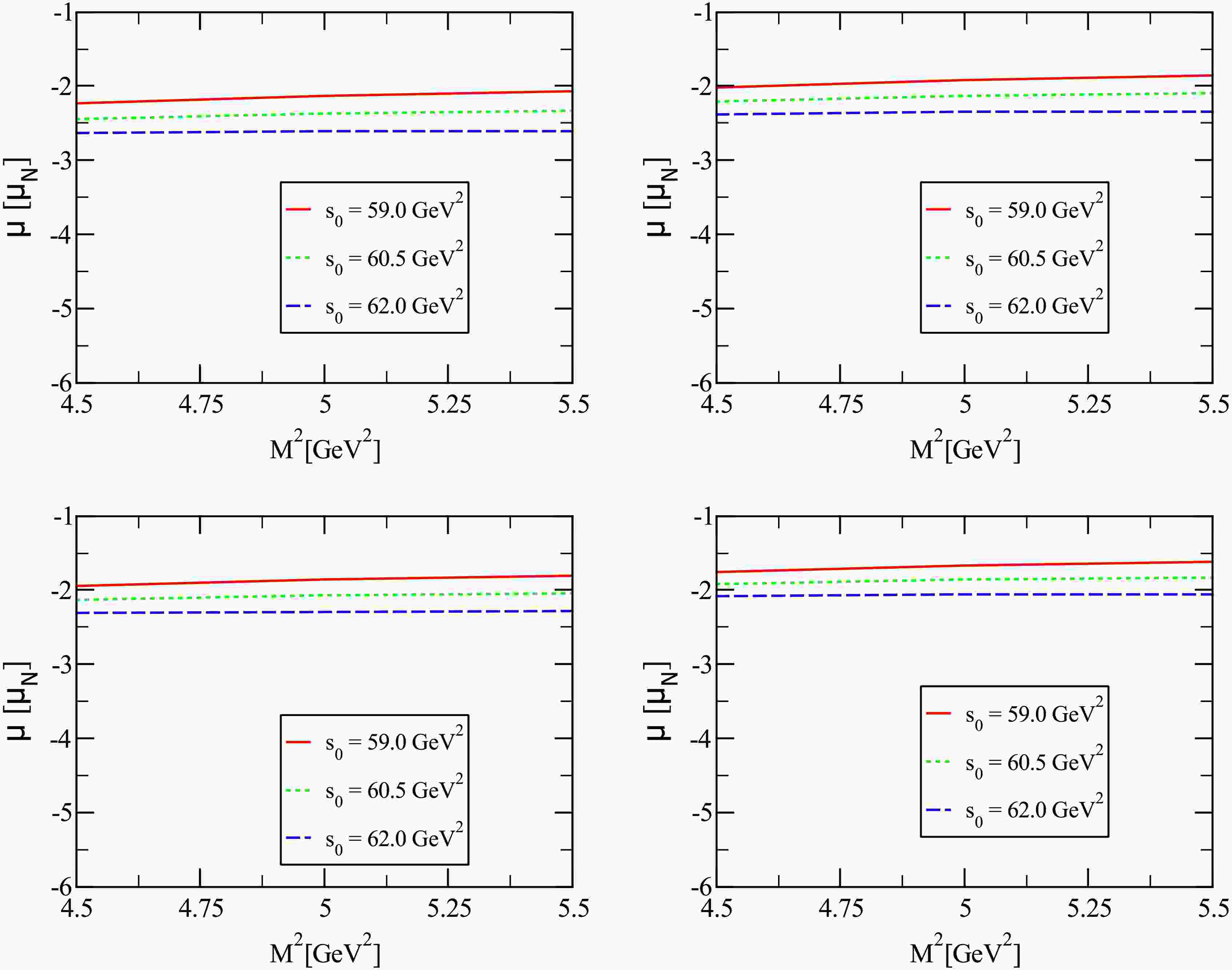
where $ \rho_i^{{\rm{Dim}} 7} ({\rm{M}}^2,{\rm{s}}_0) $ is the highest dimensional term in the OPE of $ \rho_i ({\rm{M}}^2,{\rm{s}}_0) $.

Under the above-mentioned requirements, the working windows of the supplementary parameters, as outlined in Table 2, are obtained. As observed from these results, the method satisfies the constraints. To enhance our predictions and for completeness, Fig. 1 shows the variations in the derived magnetic moments of these states with regards to M² and s₀. As shown in the figure, the magnetic moments of these states show a relatively mild dependence on these supplementary variables. At this juncture, all criteria inherent to the QCD LCSR have been fulfilled, and we expect to make reliable predictions.

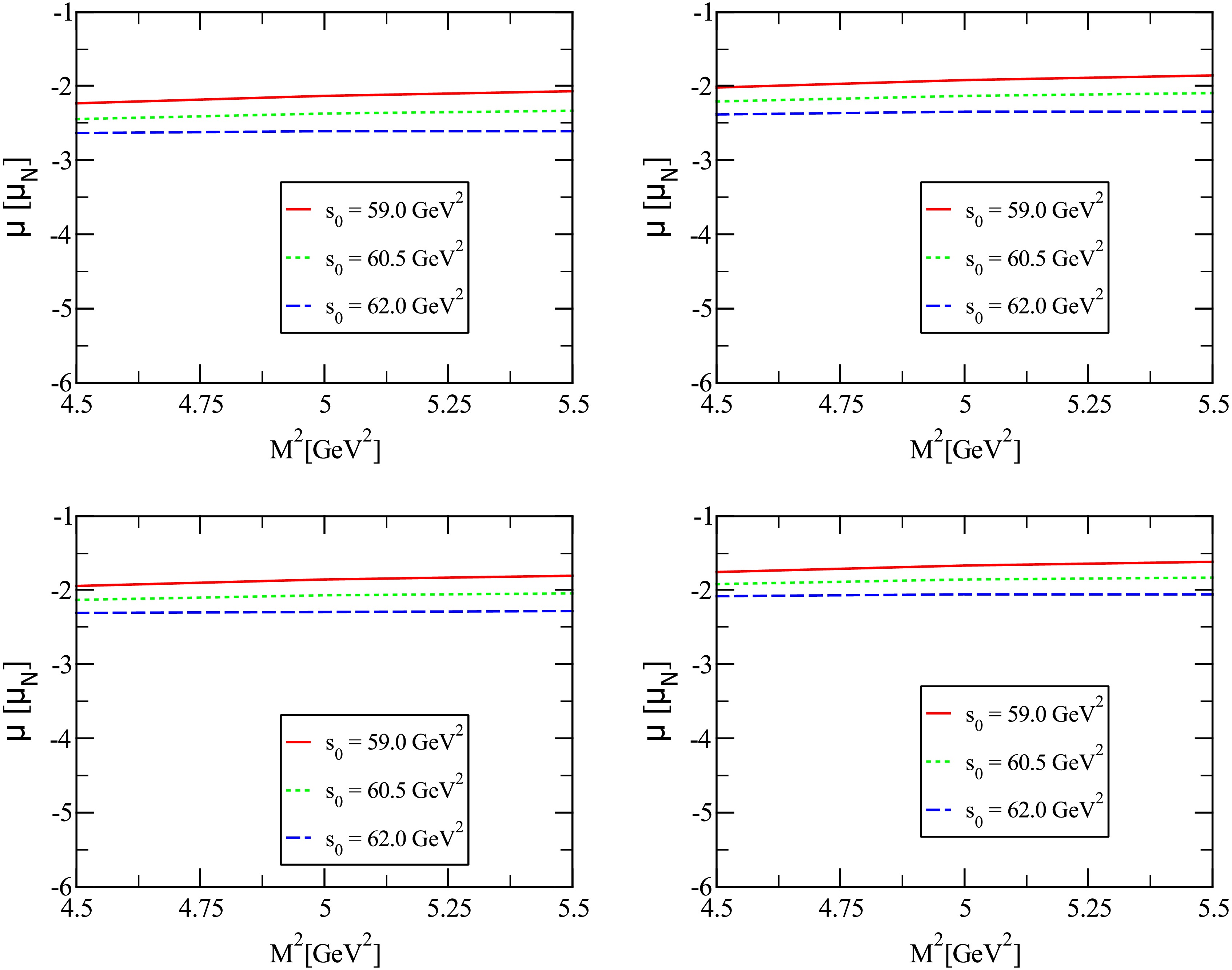
Figure 1.  (color online) Variation of magnetic moments $ Z_{\bar{b} c} $ tetraquarks as a function of the M² at different values of s₀.

The estimated magnetic moments of the $ Z_{\bar{b} c} $ tetraquark states, which take into account the ambiguities inherent in the input quantities and fluctuations in the M² and s₀ working regions, are provided in Table 2. Moreover, to enhance comprehension, we have provided the results of the magnetic moments, presented in conjunction with both their central values and errors, in Fig. 2. The uncertainties in our numerical results originate from the variations in the input parameters. The dominant sources are the continuum threshold s₀ (30%), tetraquark residue (20%), tetraquark mass (19%), and quark masses (12%). Smaller uncertainties arise from the parameters of the photon DAs (7%), Borel parameter M² (7%), and other inputs, such as various QCD condensates (5%).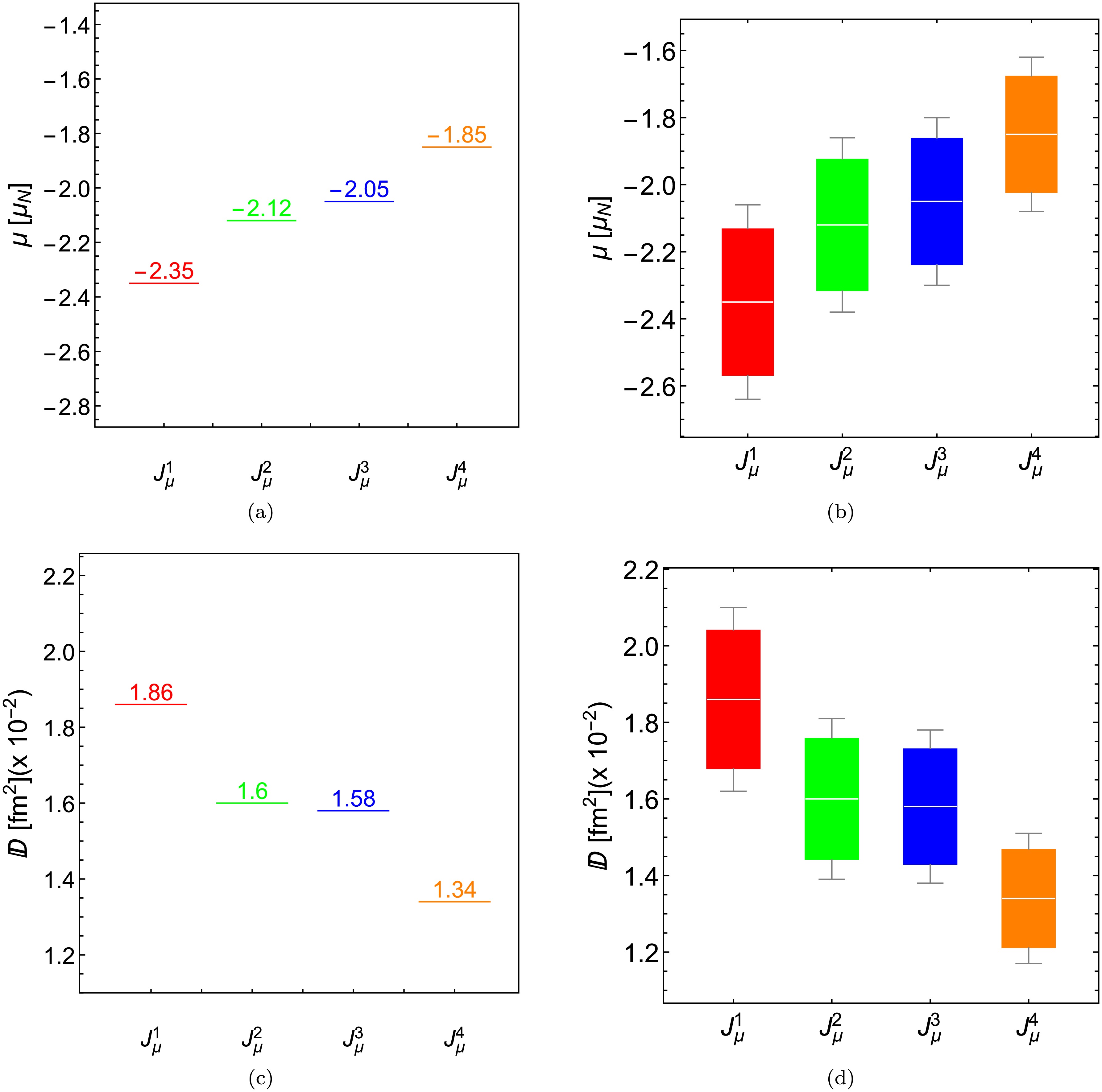

Figure 2.  (color online) Magnetic $ (\mu) $ and quadrupole ($ {\cal{D}} $) moments of $ Z_{\bar{b} c} $ tetraquark states: (a) and (c) central values; (b) and (d) combined with errors, respectively.

In consideration of the findings yielded by this study, the following observations are made:

● The main contribution of the analysis comes from the short-distance interactions of photon with quarks, which are responsible for approximately 85% of the magnetic moment results. The remaining contributions are derived from the long-distance interactions of light quarks with the photon, which is a non-perturbative contribution. The observed decomposition of contributions—approximately 85% from the short-distance photon-quark interaction and 15% from long-distance effects encoded in photon DAs—is a direct consequence of the QCD sum rule framework and provides insight into the nature of the state. In the LCSR approach, the OPE is organized by operator dimension. The dominant contribution naturally arises from the leading perturbative diagram, where the photon couples directly to a propagating quark, which is calculable within perturbative QCD. The substantial magnitude of this term confirms that our sum rule is sensitive primarily to the hard, partonic core of a compact tetraquark. The non-perturbative 15%, originating from higher-twist photon DAs, incorporates soft gluon and vacuum polarization effects that dress the photon. This modest but non-negligible share is essential: it ensures the convergence of the OPE while capturing necessary hadronic cloud effects, yet its subdominant role reinforces the picture of a compact, diquark-antidiquark object rather than an extended molecular configuration. Such a balance between perturbative and non-perturbative contributions is consistent with LCSR analyses of conventional hadrons and supports the internal consistency of our calculation.

● The numerical results presented in Table 3 reveal several important features regarding the internal quark dynamics of the $ Z_{\bar{b}c} $ states. First, the magnetic dipole moment is predominantly shaped by the contributions of the light quarks. In particular, the u quark yields a large positive contribution, while the d quark gives a comparably large negative one, partially canceling each other. The heavy quark contributions from the c and b quarks are relatively smaller in magnitude, as expected due to their larger masses, and consistently contribute with negative signs across all interpolating currents. Notably, while the u quark yields the largest individual positive contribution due to its charge and relatively light mass, this effect is substantially counterbalanced by the combined negative inputs of the d, c, and b quarks. This cancellation indicates a delicate internal structure in which spin and spatial correlations between constituent quarks significantly influence the electromagnetic properties of the state. The comparable contributions from c and d quarks, despite their $ \sim 300 $-fold mass difference, arise from the correlated spin structure of the tetraquark. The naive expectation $ \mu \propto Q/m $ is modified by the spin expectation values $ \langle S^z \rangle $ within the bound state. The light quark's large $ 1/m_d $ factor is compensated by its small spin matrix element in the spin-singlet diquark, while the charm quark's contribution is enhanced by its larger charge ($ Q_c = +2/3 $ vs $ Q_d = -1/3 $) and more favorable spin alignment in the wave function. Experimentally, such negative and moderate magnetic dipole moments could manifest in radiative transitions or influence the decay widths of the $ Z_{\bar{b}c} $ states into final states involving photons. If these states are observed in future experiments, their electromagnetic multipole moments—particularly magnetic dipole transitions to nearby tetraquark or mesonic states—may serve as indirect probes of their internal spin structure. Therefore, our results may provide guidance for designing experimental searches sensitive to electromagnetic observables in the exotic hadron sector. Overall, the magnetic dipole moment emerges not merely as a static property but as a powerful probe of the interplay between quark flavor, color dynamics, and spin correlations inside exotic hadrons. The results obtained here offer both a testable prediction and theoretical benchmark for the structure of open-flavor tetraquark states.

● Although the masses of the states with quantum numbers ${J^{P}} = 1^{+}$ are nearly identical, there is a discrepancy in the numerical results of their magnetic moments, with a difference of approximately 10%−15%. This may assist in differentiating between quantum numbers associated with states with identical quark content.

● The magnitude of the magnetic moment may be interpreted as indicating the experimental accessibility of the corresponding physical parameters. The magnitude of the results suggests that they may be measured in future experiments. The results obtained regarding the magnetic moments of the $ Z_{\bar{b} c} $ tetraquark states may be checked within the context of different phenomenological approaches.

● To the best of our knowledge, this is a pioneering study investigating the magnetic moments of ${I(J^P)} = 1(1^+)$ $ Z_{\bar{b} c} $ tetraquarks. Consequently, there is currently no available theoretical prediction or experimental data to which our numerical values can be compared. However, for illustrative purposes, we can make a comparison with the magnetic moments of ${I(J^P)} = 0(1^+)$ $ Z_{\bar{b} c} $ tetraquark states. In [39], the magnetic moments of the $ [uc] [\bar{u} \bar{b}] $ and $ [dc] [\bar{d} \bar{b}] $ tetraquark states were calculated within the framework of the LCSR method, assuming a compact tetraquark picture with a $ 6_c \otimes \bar{6}_c $ color configuration. The results obtained were $ \mu_{[uc] [\bar{u} \bar{b}]} = 3.05^{+1.18}_{-0.95} \mu_N $ and $ \mu_{[dc] [\bar{d} \bar{b}]}= 2.38^{+0.95}_{-0.75} \mu_N $. A direct comparison shows a clear numerical difference between our predictions and those of [39]. This difference originates from the fundamentally different isospin and color structures assumed in the two studies: we employ the $ 3_c \otimes \bar{3}_c $ configuration, while [39] uses the $ 6_c \otimes \bar{6}_c $ scheme. These distinct color configurations enforce different spin correlations within the diquark subsystems due to the Pauli exclusion principle. In the $ 3_c \otimes \bar{3}_c $ model used here, the light-heavy diquark $ [qc] $ is in a color antitriplet. For light quarks, this color antisymmetry typically pairs with a spin-0 (singlet) state to maintain the overall antisymmetry of the fermionic wave function. This spin-singlet structure determines specific patterns for the contributions to the magnetic moment operator. Conversely, in the $ 6_c \otimes \bar{6}_c $ configuration, the diquark is in a color sextet, which is symmetric in color. To satisfy Fermi statistics, this is naturally coupled with a spin-1 (triplet) state. This change in the internal spin alignment modifies both the individual quark spin matrix elements and interference between contributions from different quarks. Because the magnetic moment depends sensitively on the quark spin orientations as well as their charges, isospin, and masses, such a structural difference logically leads to different numerical predictions. This comparison illustrates the sensitivity of the magnetic moment to the internal color-spin structure of tetraquarks. The significant variation between predictions based on different color configurations demonstrates that electromagnetic properties such as the magnetic moment can serve as valuable discriminators between competing theoretical models of exotic hadron structure, providing complementary information to mass spectroscopy.

● As a further consequence, the quadrupole moments of these states have also been calculated, and the results are as follows:

The quadrupole moments are small in magnitude ($ |{\cal{D}}| \sim 0.01 $–0.02 fm²), while the magnetic moments are substantial ($ |\mu| \sim 1.85 $–2.35 $ \mu_N $). The non-zero quadrupole moment results for the studied states imply a deviation from spherical charge distributions. It is well established that the geometric shape of hadrons can be inferred from the sign of their quadrupole moments: a negative value corresponds to an oblate shape, whereas a positive value indicates a prolate configuration. According to predicted results, the geometric shape of these states is prolate.

The magnetic ($ \mu \sim -1.8 $ to $ -2.4\,\mu_N $) and quadrupole ($ {\cal{D}} \sim 10^{-2}\;{\rm{fm}}^2 $) moments calculated in this work provide quantitative predictions that can, in principle, be tested experimentally. This section discusses realistic pathways for such tests, with particular emphasis on how electromagnetic moments—central to this study—could be constrained through measurable observables.

The $ Z_{\bar{b}c} $ tetraquarks can be produced at both hadron and electron-positron colliders:

● LHC (LHCb): The most promising venue. The dominant mechanism is gluon fusion $ gg \to b\bar{b}c\bar{c} $ followed by hadronization. While a precise cross-section prediction requires dedicated calculations, the production of similar open-heavy-flavor states (e.g., $ B_c $ mesons) is well-established at LHCb with significant yields. Given LHCb's demonstrated capability to reconstruct states with b- and c-quarks, and with projected integrated luminosities of $ 50\,{\rm{fb}}^{-1} $ in Run 3–4, the $ Z_{\bar{b}c} $ tetraquark should be producible in sufficient numbers for discovery studies.

● Belle II: Cleaner events via $ \Upsilon(5S) $ decays, e.g., $ e^+e^- \to \Upsilon(5S) \to Z_{\bar{b}c} + \bar{D}^{(*)} + \pi $. The expected branching fractions are $ \sim 10^{-5} $–10^-4, accessible with the full Belle II dataset.

For initial discovery, hadronic decays offer the required signal yield:

● $ Z_{\bar{b}c} \to B_c^+ \pi^- $ with $ B_c^+ \to J/\psi(\to\mu^+\mu^-) \pi^+ $

● $ Z_{\bar{b}c} \to J/\psi(\to\mu^+\mu^-) K^- $

With 1% reconstruction efficiency, $ 50\;{\rm{fb}}^{-1} $ at LHCb gives $ {\cal{O}}(250) $ reconstructed events—sufficient for a $ 5\sigma $ observation.

The magnetic moment can be constrained through $ M1 $ radiative decays between spin-partner states, e.g., $ Z_{\bar{b}c}(1^+) \to Z_{\bar{b}c}(0^+) + \gamma $. The partial width is

where $ k_\gamma $ is the photon energy and $ \mu_{{\rm{trans}}} $ the transition magnetic moment. For heavy compact systems, $ \mu_{{\rm{trans}}} \approx \mu_{{\rm{static}}} $is considered to a good approximation. Using our predicted $ |\mu| \sim 2\,\mu_N $ and typical $ k_\gamma \sim 100 $ MeV, we expect $ \Gamma_{M1} \sim 0.1 $–1 keV.

Theoretical caveat: The approximation $ \mu_{{\rm{trans}}} \approx \mu_{{\rm{static}}} $ neglects possible differences in the $ 1^+ $ and $ 0^+ $ wave functions, introducing a systematic uncertainty of $ \sim 20 $%– 30% on the extracted μ from $ \Gamma_{M1} $. Full lattice QCD or model calculations of the transition form factor would be required for a precise extraction.

Experimental requirements: Measuring $ \Gamma_{M1} $ requires:

1. Reconstruction of both the initial and final tetraquark states

2. Detection of the soft photon ($ E_\gamma \sim 50 $–300 MeV)

3. Sufficient statistics: Assuming $ {\cal{B}}(Z^* \to Z\gamma)$ ~ 1% and 10% photon efficiency, $ {\cal{O}}(10^4) $ reconstructed Z events are required for a ~ 50% uncertainty on $ \Gamma_{M1} $

Experimental considerations: Detecting $ E_\gamma \sim $ 100 MeV photons requires excellent calorimeter granularity and low-energy thresholds. At LHCb, converted photons or sophisticated $ \pi^0 $ veto algorithms would be essential for background suppression.

The quadrupole moment $ {\cal{D}} $ affects the $ E2/M1 $ mixing ratio in radiative transitions. The photon angular distribution in $ Z^* \to Z\gamma $ depends on the following ratio:

where $ a_2 $ is sensitive to both μ and $ {\cal{D}} $. A precision angular analysis of cascade decays like $ Z^* \to (Z \to J/\psi\pi) + \gamma $ could, in principle, extract $ {\cal{D}} $.

If $ Z_{\bar{b}c} $ states are produced with polarization (as expected in forward LHCb acceptance), the angular distributions of decay products depend on electromagnetic form factors. While more model-dependent, such analyses provide complementary constraints.

Alternative approaches: If semileptonic decays $ Z_{\bar{b}c} \to D^{(*)} \ell \nu $ are observed, the lepton angular distribution could provide additional constraints on the magnetic form factor, though these channels are expected to have small branching fractions.

Required luminosity: Constraining μ via $ \Gamma_{M1} $ is statistically demanding. The need for $ {\cal{O}}(10^4) $ reconstructed Z events makes this an objective for the HL-LHC era ($ {\cal{L}} \gtrsim 300\,{\rm{fb}}^{-1} $) rather than earlier runs.

Primary experimental challenges:

● Soft photon reconstruction: $ M1 $ photons are soft ($ E_\gamma \sim 50 $–300 MeV) and must be distinguished from abundant $ \pi^0 \to \gamma\gamma $ backgrounds. This requires excellent calorimeter performance and advanced particle identification.

● Theoretical systematics: Extracting the static moment μ from the measured $ \Gamma_{M1} $ involves assumptions about wavefunction overlaps. The resulting ~ 20%–30% uncertainty may dominate over statistical errors.

● Background control: Combinatorial background from conventional B- and D-meson decays could obscure both the tetraquark signals and radiative photons.

Realistic timeline: Discovery via hadronic decay channels is feasible with current LHCb datasets. A first measurement of the radiative width $ \Gamma_{M1} $ may be possible by the end of LHC Run 4, while precise electromagnetic moment extraction will likely require HL-LHC statistics.

This study provides specific numerical predictions for the electromagnetic properties of $ Z_{\bar{b}c} $ tetraquarks. While challenging, experimental verification is grounded in established techniques: radiative transition measurements and angular analyses. A confirmed magnetic moment around $ -2\,\mu_N $ would provide strong evidence for the compact diquark-antidiquark structure proposed here, offering a clear discriminant against molecular interpretations where different charge and spin distributions would likely yield different magnetic responses. The coming decade of high-luminosity heavy-flavor experiments will be crucial for testing these predictions and advancing our understanding of exotic hadron structure.

An investigation of the electromagnetic characteristics of unconventional states may offer new insights into their internal structures. In particular, the magnetic moment characteristics may serve as a crucial physical observable for differentiating exotic states with disparate configurations or spin-parity quantum numbers. As a promising avenue for research, encompassing both opportunities and challenges, an in-depth examination of the electromagnetic properties of exotic states is crucial for advancing our understanding of unconventional states. Motivated by this, in this study, the magnetic moments of ${I(J^{P})} = 1(1^{+ })$ $ Z_{\bar{b} c} $ tetraquark states are analyzed in the framework of QCD LCSR by considering the diquark-antidiquark approximation. Despite the nearly identical masses of the tetraquark states analyzed in this study, significant differences are observed in their magnetic moments. This may facilitate the differentiation between quantum numbers associated with states with identical quark content. The results show that heavy quarks overcoming light quarks can determine both the sign and magnitude of the magnetic moments of these tetraquark states. The numerical results obtained in this study suggest that the magnetic moments of $ Z_{\bar{b} c} $ tetraquark states may reveal aspects of their underlying structure, which could in turn distinguish between their spin-parity quantum numbers and internal structure. The results obtained regarding the magnetic moments of the $ Z_{\bar{b} c} $ tetraquark states may be checked within the context of different phenomenological approaches. As a further consequence, the quadrupole moments of these states have also been calculated. The quadrupole moment results obtained for these states are non-zero, indicating the presence of a non-spherical charge distribution.

The magnetic moment of hadrons constitutes an indispensable component in the calculation of the photo- and electro-production cross-sections. In the future, this parameter may be derived from experimental data. As the luminosity of future runs increases, it will become possible to extract spectroscopic properties and magnetic moments of $ Z_{\bar{b} c} $ tetraquark states from experimental facilities. This will facilitate the distinction between different theoretical configurations and contribute to a deeper understanding of the dynamics that govern their formation. Furthermore, it will be essential to determine the branching ratios of the various decay modes and decay channels of $ Z_{\bar{b} c} $ tetraquark states.

In this Appendix, we provide the full analytical results for the magnetic moment calculations corresponding to the interpolating current $ J_\mu^1 $. The explicit expressions are as follows:

where the $ I[n,m] $, and $ I_i[{\cal{F}}] $ functions are expressed as

where $ {\cal{M}} = (m_c+m_b)^2 $, and $ {\cal{F}} $ denotes the relevant DAs of the photon.

In this Appendix, we provide the matrix elements $ \langle \gamma(q) | \bar{q}(x) \Gamma_i q(0) | 0 \rangle $ and $ \langle \gamma(q) | \bar{q}(x) \Gamma_i G_{\mu\nu} q(0) | 0 \rangle $, which are associated with the photon DAs, as derived in [85]:

where $ \varphi_\gamma(u) $ is the DA of leading twist-2; $ \psi^v(u) $, $ \psi^a(u) $, $ {\cal{A}}(\alpha_i) $, and $ {\cal{V}}(\alpha_i) $ are the twist-3 amplitudes; and $ h_\gamma(u) $, $ \mathbb{A}(u) $, $ {\cal{S}}(\alpha_i) $, $ {\cal{\tilde{S}}}(\alpha_i) $, $ {\cal{T}}_1(\alpha_i) $, $ {\cal{T}}_2(\alpha_i) $, $ {\cal{T}}_3(\alpha_i) $, and $ {\cal{T}}_4(\alpha_i) $ are the twist-4 photon DAs. The measure $ {\cal{D}} \alpha_i $ is defined as

The forms of the DAs that are incorporated into the matrix elements above are given by

where $ \varphi_2(1\; GeV) = 0 $, $ w^V_\gamma = 3.8 \pm 1.8 $, $ w^A_\gamma = -2.1 \pm 1.0 $, $ \kappa = 0.2 $, $ \kappa^+ = 0 $, $ \zeta_1 = 0.4 $, and $ \zeta_2 = 0.3 $.