


 Abstract
 HTML
HTML Reference
 Related
 PDF
PDF


-
The precise calculation of nuclear mass is of profound significance in the fields of nuclear physics and astrophysics [1, 2]. Measuring the mass of singular nuclei [3] and improving their accuracy [4, 5] is a long-term process. However, the present experimental facilities aimed at the nuclear mass are still not accessible to these short-lived nuclei in the r-process path[6]. As a result, the theoretical mass evaluations are urgently required especially towards the high-precision extrapolation. Several nuclear mass models have been developed to achieve root-mean-square deviations (RMSDs) ranging from several hundred keV to a few MeV for all known nuclear masses.
The study of nuclear mass models traces back to the early 20th century when Gamow proposed the liquid drop model for nuclear binding energy based on nuclear force saturation [7], upon which the Weizsäcker formula was established as a macroscopic semi-empirical formulation [8, 9]. Möller [10−12] and Haustein [13] incorporated microscopic effects into the liquid drop framework, developing the Finite-Range Droplet Model (FRDM). Classified as macro-micro models, analogous approaches include the extended Bethe-Weizsäcker (BW2) mass formula [14, 15], Weizsäcker-Skyrme (WS) mass formula [16−20], and Duflo-Zuker (DZ) mass formula [21]. Microscopic theoretical models derive nuclear binding energies through approximate solutions of many-body equations from effective nucleon-nucleon interactions, exemplified by the Hartree-Fock-Bogoliubov (HFB) model and relativistic mean-field mass model [22, 23].
For conceptual clarity, scholars categorize these theoretical frameworks into three classes: global mass models encompassing comprehensive theories, local models deriving target nuclear masses from adjacent known nuclei, and regional models describing nuclear quantity relationships within specific domains [24]. Typical regional models comprise the Isobaric Multiplet Mass Equation (IMME) [25, 26] and mirror nucleus mass formulae [27, 28]. Prominent local models include the Garvey-Kelson (GK) relations [29, 30] and proton-neutron interaction mass relations(
$ \delta V_{in-jp} $ )[31, 32].Conventional mass models relying on empirical parameters exhibit notable discrepancies in mass predictions for nuclei far from the β stability line, necessitating enhanced extrapolation capabilities in nuclear mass modeling. Recent advances in machine learning have enabled data-driven approaches for nuclear mass predictions, opening new avenues through neural network-optimized models [33−35], fission yield distributions [36], and decay energy studies [37]. Additionally,the physics-informed neural network (PINN) method has recently attracted significant attention in nuclear mass research [38]. Furthermore, radial basis functions (RBF) [19, 20] and uncertainty quantification methodologies [39, 40] have significantly improved the precision of theoretical models in characterizing and predicting nuclear ground-state properties.
Uncertainty analysis in scientific modeling has gained paramount importance, particularly in physics and engineering disciplines. Conventional phenomenological approaches like least squares methods predominantly focus on experimental data fitting while neglecting intrinsic model errors and parameter correlations, thereby failing to fully capture model veracity. Systematic analysis of nuclear mass model parameter uncertainties and their correlations can substantially enhance theoretical prediction accuracy, error estimation reliability, and extrapolation robustness.
Current theoretical modeling practices predominantly focus on parameter uncertainty analysis through least squares fitting, while systematic investigation of model errors remains underdeveloped. This study conducts comprehensive nuclear mass investigations under uncertainty theory framework, accounting for both statistical errors in experimental binding energies and model deficiencies, while simultaneously analyzing parameter uncertainties [41−44]. Parameter errors were quantified via Monte Carlo sampling techniques, with inter-parameter correlations analyzed [41, 44−48] to evaluate their impacts on binding energy calculation accuracy.
The remainder of this paper is organized as follows. Section II presents the selected mass formula. Section III provides a concise overview of the quantitative evaluation framework for parameter uncertainty. Building upon [47], Section IV conducts in-depth explorations of parameter correlations and optimization comparisons, with Section V concluding the study.
-
The precise calculation of nuclear mass is of profound significance in the fields of nuclear physics and astrophysics [1, 2]. Measuring the mass of singular nuclei [3] and improving their accuracy [4−7] is a long-term process. However, the present experimental facilities aimed at nuclear mass are still not accessible to these short-lived nuclei in the r-process path [8]. As a result, theoretical mass evaluations are urgently required, especially toward high-precision extrapolation. Several nuclear mass models have been developed to achieve root-mean-square deviations (RMSDs) ranging from several hundred keV to a few MeV for all known nuclear masses.
The study of nuclear mass models traces back to the early 20th century when Gamow proposed the liquid drop model for nuclear binding energy based on nuclear force saturation [9], upon which the Weizsäcker formula was established as a macroscopic semi-empirical formulation [10, 11]. Möller [12−14] and Haustein [15] incorporated microscopic effects into the liquid drop framework, developing the Finite-Range Droplet Model (FRDM). Classified as macro-micro models, analogous approaches include the extended Bethe-Weizsäcker (BW2) mass formula [16, 17], Weizsäcker-Skyrme (WS) mass formula [18−22], and Duflo-Zuker (DZ) mass formula [23]. Microscopic theoretical models derive nuclear binding energies through approximate solutions of many-body equations from effective nucleon-nucleon interactions, exemplified by the Hartree-Fock-Bogoliubov (HFB) model and relativistic mean-field mass model [24, 25].
For conceptual clarity, scholars categorize these theoretical frameworks into three classes: global mass models encompassing comprehensive theories, local models deriving target nuclear masses from adjacent known nuclei, and regional models describing nuclear quantity relationships within specific domains. Typical regional models include the Isobaric Multiplet Mass Equation (IMME) [26–27] and mirror nucleus mass formulae [28–29]. Prominent local models include the Garvey-Kelson (GK) relations [30–31] and proton-neutron interaction mass relations (
$ \delta V_{in-jp} $ ) [32–33].Conventional mass models relying on empirical parameters exhibit notable discrepancies in mass predictions for nuclei far from the β stability line, necessitating enhanced extrapolation capabilities in nuclear mass modeling. Recent advances in machine learning have enabled data-driven approaches for nuclear mass predictions, opening new avenues through neural network-optimized models [34−36], fission yield distributions [37], and decay energy studies [38]. Additionally, the physics-informed neural network (PINN) has recently attracted significant attention in nuclear mass research [39]. Furthermore, radial basis functions (RBFs) [21–22] and uncertainty quantification methodologies [40–41] have significantly improved the precision of theoretical models in characterizing and predicting nuclear ground-state properties.
Uncertainty analysis in scientific modeling has reached paramount importance, particularly in physics and engineering disciplines. Conventional phenomenological approaches, such as least squares methods, predominantly focus on experimental data fitting while neglecting intrinsic model errors and parameter correlations, thereby failing to fully capture model veracity. Systematic analysis of nuclear mass model parameter uncertainties and their correlations can substantially enhance theoretical prediction accuracy, error estimation reliability, and extrapolation robustness.
Current theoretical modeling practices predominantly focus on parameter uncertainty analysis through least squares fitting, while systematic investigations of model errors remain underdeveloped. This study conducted comprehensive nuclear mass investigations under the uncertainty theory framework, accounting for both statistical errors in experimental binding energies and model deficiencies while simultaneously analyzing parameter uncertainties [42−45]. Parameter errors were quantified via Monte Carlo sampling techniques, with inter-parameter correlations analyzed [42, 45−49] to evaluate their impacts on binding energy calculation accuracy.
The remainder of this paper is organized as follows. Section II presents the selected mass formula. Section III provides a concise overview of the quantitative evaluation framework for parameter uncertainty. Building upon Ref. [48], Section IV conducts in-depth explorations of parameter correlations and optimization comparisons, with Section V concluding the paper.
-
The mass formula BW3 is based on the classical liquid-drop model and incorporates additional physical terms for a more comprehensive analysis.
The model used in this study is from Ref. [50]:
$\begin{aligned}[b] BE_{BW3} =\; & \alpha_{v}A+\alpha_{s}A^{\frac{2}{3}}+\alpha_{C}\frac{Z^2}{A^{\frac{1}{3}}}+\alpha_{t}\frac{(N-Z)^2}{A} \\ & + \alpha_{xC}\frac{Z^{\frac{4}{3}}}{A^{\frac{1}{3}}}+\alpha_{W}\frac{|N-Z|}{A}+\alpha_{st}\frac{(N-Z)^2}{A^{\frac{4}{3}}} \\ & + \alpha_{p}\frac{\delta(N,Z)}{A^\frac{1}{2}}+\alpha_{R}A^{\frac{1}{3}}+\alpha_{m}P+\beta_{m}P^{2} \\ & + \alpha_{b}\frac{{{{(N - Z)}^4}}}{{A^3}}, \end{aligned} $
(1) where
$ \alpha_{i} $ denotes free parameters determined by fitting the experimental nuclear masses. This formula includes the exchange Coulomb term$ \alpha_{xC}\frac{Z^{\frac{4}{3}}}{A^{\frac{1}{3}}} $ , Wigner term$ \alpha_{W}\frac{|N-Z|}{A} $ , surface symmetry term$ \alpha_{st}\frac{(N-Z)^2}{A^{\frac{4}{3}}} $ , pairing term$ \alpha_{p}\frac{\delta(N,Z)}{A^\frac{1}{2}} $ , curvature term$ \alpha_{R}A^{\frac{1}{3}} $ , shell effect term$ \alpha_{m}P+\beta_{m}P^{2} $ , and fourth-order term of symmetry energy$ \alpha_{b}\frac{{{{(N - Z)}^4}}}{{A^3}} $ . It should be noted that the shell effect term contains two parameters:In equation
$ \delta(N,Z) = \frac{(-1)^N+(-1)^Z}{2} , $
(2) it takes the value
$ +1 $ for even–even nuclei,$ -1 $ for odd–odd nuclei, and$ 0 $ for odd nuclei.For P in equation (1),
$ P = \frac{\nu_n\nu_p}{\nu_n+\nu_p}, $
(3) where
$ \nu_n $ and$ \nu_p $ are the numbers of valence nucleons (the difference between the actual nucleon numbers N and Z, respectively, and the nearest magic numbers). To calculate P, the magic numbers were the canonical 2, 8, 20, 28, 50, 82, 126, and 184 for both neutrons and protons.The latest and most comprehensive database of nuclear masses is the Atomic Mass Evaluation Database, commonly known as AME2020 [51]. This tabulation served as the experimental data for the present study. The pertinent input comprises a list of measured binding energies of the nuclei acquired by multiplying the tabulated binding energy per nucleon by the mass number
$ (A) $ .Eq. (1) can be expressed in the form of a matrix
$ {{\boldsymbol{B}}_{Th}} = \boldsymbol{F}\boldsymbol{p}, $
(4) where
$ \boldsymbol{B} $ and$ \boldsymbol{p} $ are column vectors, representing the calculated value of the binding energy and coefficient corresponding to the formula, respectively.The matrix F is defined as
$\begin{array}{*{20}{l}} \boldsymbol{F}=\left( \begin{array}{cccc}{\dfrac{\partial B_{Th,1}}{\partial p_{1}}} & {\dfrac{\partial B_{Th,1}}{\partial p_{2}}} & {\cdots} & {\dfrac{\partial B_{Th,1}}{\partial p_{Np}}}\\ {\dfrac{\partial B_{Th,2}}{\partial p_{1}}} & {\dfrac{\partial B_{Th,2}}{\partial p_{2}}} & {\cdots} & {\dfrac{\partial B_{Th,2}}{\partial p_{Np}}}\\ {\vdots} & {\vdots} & {\ddots} & {\vdots}\\ {\dfrac{\partial B_{Th,Nn}}{\partial p_{1}}} & {\dfrac{\partial B_{Th,Nn}}{\partial p_{2}}} & {\cdots} & {\dfrac{\partial B_{Th,Nn}}{\partial p_{Np}}} \end{array}\right), \end{array} $
(5) where the row and column dimensions correspond to the number of nuclides and total number of parameters, respectively.
The criteria for evaluating the quality of a semi-empirical mass formula hinge on its capacity to embody clear physical principles, minimize the dependency on extraction parameters, obtain superior calculation results, and clarify nuclear properties relevant to the nuclear mass. The goodness of fit was assessed using the RMSD of the extraction from the measured binding energies as follows:
$ RMS = \sqrt{{\frac{\sum_{i}(M_i-E_i)^2}{n}}}, $
(6) where
$ M_i $ is the theoretical value,$ E_i $ is the experimental value, and n is the total number of data points. -
The mass formula BW3 is based on the classical liquid-drop model and incorporates additional physical terms for a more comprehensive analysis.
The model used in this study is from Ref. [50]:
$\begin{aligned}[b] BE_{BW3} =\; & \alpha_{v}A+\alpha_{s}A^{\frac{2}{3}}+\alpha_{C}\frac{Z^2}{A^{\frac{1}{3}}}+\alpha_{t}\frac{(N-Z)^2}{A} \\ & + \alpha_{xC}\frac{Z^{\frac{4}{3}}}{A^{\frac{1}{3}}}+\alpha_{W}\frac{|N-Z|}{A}+\alpha_{st}\frac{(N-Z)^2}{A^{\frac{4}{3}}} \\ & + \alpha_{p}\frac{\delta(N,Z)}{A^\frac{1}{2}}+\alpha_{R}A^{\frac{1}{3}}+\alpha_{m}P+\beta_{m}P^{2} \\ & + \alpha_{b}\frac{{{{(N - Z)}^4}}}{{A^3}}, \end{aligned} $
(1) where
$ \alpha_{i} $ denotes free parameters determined by fitting the experimental nuclear masses. This formula includes the exchange Coulomb term$ \alpha_{xC}\frac{Z^{\frac{4}{3}}}{A^{\frac{1}{3}}} $ , Wigner term$ \alpha_{W}\frac{|N-Z|}{A} $ , surface symmetry term$ \alpha_{st}\frac{(N-Z)^2}{A^{\frac{4}{3}}} $ , pairing term$ \alpha_{p}\frac{\delta(N,Z)}{A^\frac{1}{2}} $ , curvature term$ \alpha_{R}A^{\frac{1}{3}} $ , shell effect term$ \alpha_{m}P+\beta_{m}P^{2} $ , and fourth-order term of symmetry energy$ \alpha_{b}\frac{{{{(N - Z)}^4}}}{{A^3}} $ . It should be noted that the shell effect term contains two parameters:In equation
$ \delta(N,Z) = \frac{(-1)^N+(-1)^Z}{2} , $
(2) it takes the value
$ +1 $ for even–even nuclei,$ -1 $ for odd–odd nuclei, and$ 0 $ for odd nuclei.For P in equation (1),
$ P = \frac{\nu_n\nu_p}{\nu_n+\nu_p}, $
(3) where
$ \nu_n $ and$ \nu_p $ are the numbers of valence nucleons (the difference between the actual nucleon numbers N and Z, respectively, and the nearest magic numbers). To calculate P, the magic numbers were the canonical 2, 8, 20, 28, 50, 82, 126, and 184 for both neutrons and protons.The latest and most comprehensive database of nuclear masses is the Atomic Mass Evaluation Database, commonly known as AME2020 [51]. This tabulation served as the experimental data for the present study. The pertinent input comprises a list of measured binding energies of the nuclei acquired by multiplying the tabulated binding energy per nucleon by the mass number
$ (A) $ .Eq.(1) can be expressed in the form of a matrix
$ {{\boldsymbol{B}}_{Th}} = \boldsymbol{F}\boldsymbol{p}, $
(4) where
$ \boldsymbol{B} $ and$ \boldsymbol{p} $ are column vectors, representing the calculated value of the binding energy and coefficient corresponding to the formula, respectively.The matrix F is defined as
$\begin{array}{*{20}{l}} \boldsymbol{F}=\left( \begin{array}{cccc}{\dfrac{\partial B_{Th,1}}{\partial p_{1}}} & {\dfrac{\partial B_{Th,1}}{\partial p_{2}}} & {\cdots} & {\dfrac{\partial B_{Th,1}}{\partial p_{Np}}}\\ {\dfrac{\partial B_{Th,2}}{\partial p_{1}}} & {\dfrac{\partial B_{Th,2}}{\partial p_{2}}} & {\cdots} & {\dfrac{\partial B_{Th,2}}{\partial p_{Np}}}\\ {\vdots} & {\vdots} & {\ddots} & {\vdots}\\ {\dfrac{\partial B_{Th,Nn}}{\partial p_{1}}} & {\dfrac{\partial B_{Th,Nn}}{\partial p_{2}}} & {\cdots} & {\dfrac{\partial B_{Th,Nn}}{\partial p_{Np}}} \end{array}\right), \end{array} $
(5) where the row and column dimensions correspond to the number of nuclides and total number of parameters, respectively.
The criteria for evaluating the quality of a semi-empirical mass formula hinge on its capacity to embody clear physical principles, minimize the dependency on extraction parameters, obtain superior calculation results, and clarify nuclear properties relevant to the nuclear mass. The goodness of fit was assessed using the RMSD of the extraction from the measured binding energies as follows:
$ RMS = \sqrt{{\frac{\sum_{i}(M_i-E_i)^2}{n}}}, $
(6) where
$ M_i $ is the theoretical value,$ E_i $ is the experimental value, and n is the total number of data points. -
The mass formula BW3 is based on the classical liquid-drop model and incorporates additional physical terms for a more comprehensive analysis.
The model used in this study is obtained from Ref. [49]:
$\begin{aligned}[b] BE_{BW3} =\; & \alpha_{v}A+\alpha_{s}A^{\frac{2}{3}}+\alpha_{C}\frac{Z^2}{A^{\frac{1}{3}}}+\alpha_{t}\frac{(N-Z)^2}{A} \\ & + \alpha_{xC}\frac{Z^{\frac{4}{3}}}{A^{\frac{1}{3}}}+\alpha_{W}\frac{|N-Z|}{A}+\alpha_{st}\frac{(N-Z)^2}{A^{\frac{4}{3}}} \\ & + \alpha_{p}\frac{\delta(N,Z)}{A^\frac{1}{2}}+\alpha_{R}A^{\frac{1}{3}}+\alpha_{m}P+\beta_{m}P^{2} \\ & + \alpha_{b}\frac{{{{(N - Z)}^4}}}{{A^3}}, \end{aligned} $

(1) where
$ \alpha_{i} $ denotes free parameters determined by fitting the experimental nuclear masses. In this formula, the exchange Coulomb term$ \alpha_{xC}\frac{Z^{\frac{4}{3}}}{A^{\frac{1}{3}}} $ , Wigner term$ \alpha_{W}\frac{|N-Z|}{A} $ , surface symmetry term$ \alpha_{st}\frac{(N-Z)^2}{A^{\frac{4}{3}}} $ , pairing term$ \alpha_{p}\frac{\delta(N,Z)}{A^\frac{1}{2}} $ , curvature term$ \alpha_{R}A^{\frac{1}{3}} $ , shell effect term$ \alpha_{m}P+\beta_{m}P^{2} $ , and fourth-order term of symmetry energy$ \alpha_{b}\frac{{{{(N - Z)}^4}}}{{A^3}} $ have been added. It should be noted that the shell effect term contains two parameters.In equation
$ \delta(N,Z) = \frac{(-1)^N+(-1)^Z}{2} , $

(2) it takes the value
$ +1 $ for even–even nuclei,$ -1 $ for odd–odd nuclei, and$ 0 $ for odd nuclei.For P in equation (1),
$ P = \frac{\nu_n\nu_p}{\nu_n+\nu_p}, $

(3) where
$ \nu_n $ and$ \nu_p $ are the numbers of valence nucleons (the difference between the actual nucleon numbers N and Z respectively, and the nearest magic numbers). To calculate P, the magic numbers were the canonical 2, 8, 20, 28, 50, 82,126, and 184 for both neutrons and protons.The latest and most comprehensive database of nuclear masses is the Atomic Mass Evaluation Database, commonly known as AME2020 [50]. This tabulation served as the experimental data for the present study. The pertinent input comprises a list of measured binding energies of the nuclei acquired by multiplying the tabulated binding energy per nucleon by the mass number
$ (A) $ .Eq.(1) can be expressed in the form of a matrix
$ {{{B}}_{Th}} = {F}{p}, $

(4) where
$ {B} $ and$ {p} $ are column vectors, representing the calculated value of the binding energy and the coefficient corresponding to the formula respectively.The matrix F is defined as
$\begin{array}{*{20}{l}} {F}=\left( \begin{array}{cccc}{\dfrac{\partial B_{Th,1}}{\partial p_{1}}} & {\dfrac{\partial B_{Th,1}}{\partial p_{2}}} & {\cdots} & {\dfrac{\partial B_{Th,1}}{\partial p_{Np}}}\\ {\dfrac{\partial B_{Th,2}}{\partial p_{1}}} & {\dfrac{\partial B_{Th,2}}{\partial p_{2}}} & {\cdots} & {\dfrac{\partial B_{Th,2}}{\partial p_{Np}}}\\ {\vdots} & {\vdots} & {\ddots} & {\vdots}\\ {\dfrac{\partial B_{Th,Nn}}{\partial p_{1}}} & {\dfrac{\partial B_{Th,Nn}}{\partial p_{2}}} & {\cdots} & {\dfrac{\partial B_{Th,Nn}}{\partial p_{Np}}} \end{array}\right), \end{array} $

(5) The row and column dimensions of matrix F correspond to the number of nuclides and the total number of parameters, respectively.
The criteria for evaluating the quality of a semi-empirical mass formula hinge on its capacity to embody clear physical principles, minimize the dependency on extraction parameters, obtain superior calculation results, and clarify nuclear properties relevant to the nuclear mass. The goodness of fit was assessed using the RMSD of the extraction from the measured binding energies, as follows:
$ RMS = \sqrt{{\frac{\sum_{i}(M_i-E_i)^2}{n}}}, $

(6) where
$ M_i $ is the theoretical value,$ E_i $ is the experimental value, and n is the total number of data points. -
In the literature related to the liquid drop model, the least-squares method is typically the favored method to determine the parameters. This method aims to minimize the sum of the squared errors:
$ {\chi}^2 = {\sum\limits_{i = 1}^{{N_n}} {[{E_i} - {}_{{Z_i}}^{{A_i}}B({\alpha _v},{\alpha _s}, \cdots ,{\beta _m},{\alpha _b})]} ^2}, $
(7) where
$ {N_n} $ is the total number of selected nuclides,$ {E_i} $ is the experimental binding energy of the nuclide, and$ {B_i} $ is the theoretical binding energy of the nuclide.The previous expression can be written in matrix form as
$ \chi^2(\boldsymbol{p})= \left\| \boldsymbol{Fp}-\boldsymbol{B}_{\mathrm{Exp}} \right\| _2^2, $
(8) and its minimization with respect to the parameters yields the following solution:
$ \boldsymbol{p}=(\boldsymbol{F}^T\boldsymbol{F})^{-1}\boldsymbol{F}^T\boldsymbol{B}_{\mathrm{Exp}}. $
(9) -
In the literature related to liquid drop model, the least-squares method is, more often than not, the favored method to determine the parameters. This method consists in minimizing the sum of the squared errors,
$ {\chi}^2 = {\sum\limits_{i = 1}^{{N_n}} {[{E_i} - {}_{{Z_i}}^{{A_i}}B({\alpha _v},{\alpha _s}, \cdots ,{\beta _m},{\alpha _b})]} ^2}, $

(7) where
$ {N_n} $ is the total number of selected nuclides,$ {E_i} $ is the experimental binding energy of the nuclide, and$ {B_i} $ is the theoretical binding energy of the nuclide.The previous expression can be written in matrix form,
$ {\chi}^2({{p}}) = \left\| {{{Fp}} - {{{B}}_{Exp}}} \right\|_2^2, $

(8) and its minimization with respect to the parameters yields the following solution:
$ {{p}} = {({{{F}}^T}{{F}})^{ - 1}}{{{F}}^T}{{{B}}_{Exp}}. $

(9) -
The Monte Carlo Bootstrap Method is a statistical resampling technique widely applied in parameter estimation, uncertainty analysis, and model validation. Its fundamental principle involves resampling from an original dataset with a specified estimator to construct new dataset series, forming a bootstrap sample set. Empirical parameter distributions can be derived through analysis of individual bootstrap samples.
Nuclear mass formulae typically contain multiple empirical parameters that are determined by fitting experimental data. Parameter values inherently contain uncertainties that propagate from these experimental errors. This study investigated parameter distributions by performing random sampling through the Monte Carlo bootstrap method, generating numerous pseudo-datasets that incorporate statistical errors in experimental binding energies to estimate parameter uncertainties. The specific implementation procedure comprises the following steps:
1. The difference between the experimental and calculated values of the binding energy is taken as the initial set and denoted as
$ \varepsilon (A) $ . In total, there are M = 3250 nuclides (excluding nuclides with N and Z less than 7). By using the method of resampling, M samples can be extracted from the initial set$ \varepsilon (A) $ to obtain a sample set$ \varepsilon^{*}(A) $ , thereby obtaining a new set of experimental values:$ B_{\mathrm{Exp}}^*(N,Z)=B_{\mathrm{Exp}}(N,Z)+\varepsilon^*(N,Z). $
(10) 2. Using
$ B_{\mathrm{Exp}}^*(N,Z) $ as the new input for least squares, a set of parameters is obtained.3. Repeating the self-sampling
$ T=5000 $ times, one can obtain the empirical distribution of the parameters.4. Using the obtained parameter set, uncertainty evaluation and correlation analysis among each parameter item are conducted.
-
The Monte Carlo Bootstrap Method is a statistical resampling technique widely applied in parameter estimation, uncertainty analysis, and model validation. Its fundamental principle involves resampling from an original dataset with a specified estimator to construct new dataset series, forming a bootstrap sample set. Empirical parameter distributions can be derived through analysis of individual bootstrap samples.
Nuclear mass formulae typically contain multiple empirical parameters that are determined by fitting experimental data. Parameter values inherently contain uncertainties that propagate from these experimental errors. This study investigates parameter distributions by performing random sampling through the Monte Carlo bootstrap method, generating numerous pseudo-datasets that incorporate statistical errors in experimental binding energies to estimate parameter uncertainties. The specific implementation procedure comprises the following steps:
1. The difference between the experimental value and the calculated value of the binding energy is taken as the initial set and denoted as
$ \varepsilon (A) $ . In total, there are M = 3250 nuclides (excluding nuclides with N and Z less than 7). By using the method of resampling, M samples can be extracted from the initial set$ \varepsilon (A) $ to obtain a sample set$ \varepsilon^{*}(A) $ , thereby obtaining a new set of experimental values:$ B_{Exp}^*(N,Z) = {B_{Exp}}(N,Z) + \varepsilon^{*}(N,Z). $

(10) 2. Using
$ B_{Exp}^*(N,Z) $ as the new input for least squares, a set of parameters is obtained.3. Repeating the self-sampling for
$ T=5000 $ times, one can obtain the empirical distribution of the parameters.4. Using the obtained parameter set, uncertainty evaluation and correlation analysis among each parameter item are carried out.
-
The Monte Carlo Bootstrap Method is a statistical resampling technique widely applied in parameter estimation, uncertainty analysis, and model validation. Its fundamental principle involves resampling from an original dataset with a specified estimator to construct new dataset series, forming a bootstrap sample set. Empirical parameter distributions can be derived through analysis of individual bootstrap samples.
Nuclear mass formulae typically contain multiple empirical parameters that are determined by fitting experimental data. Parameter values inherently contain uncertainties that propagate from these experimental errors. This study investigated parameter distributions by performing random sampling through the Monte Carlo bootstrap method, generating numerous pseudo-datasets that incorporate statistical errors in experimental binding energies to estimate parameter uncertainties. The specific implementation procedure comprises the following steps:
1. The difference between the experimental and calculated values of the binding energy is taken as the initial set and denoted as
$ \varepsilon (A) $ . In total, there are M = 3250 nuclides (excluding nuclides with N and Z less than 7). By using the method of resampling, M samples can be extracted from the initial set$ \varepsilon (A) $ to obtain a sample set$ \varepsilon^{*}(A) $ , thereby obtaining a new set of experimental values:$ B_{\mathrm{Exp}}^*(N,Z)=B_{\mathrm{Exp}}(N,Z)+\varepsilon^*(N,Z). $
(10) 2. Using
$ B_{\mathrm{Exp}}^*(N,Z) $ as the new input for least squares, a set of parameters is obtained.3. Repeating the self-sampling
$ T=5000 $ times, one can obtain the empirical distribution of the parameters.4. Using the obtained parameter set, uncertainty evaluation and correlation analysis among each parameter item are conducted.
-
The BW3 mass formula was constructed through multivariate regression analysis with 12 independent variables, whose statistical properties are susceptible to multicollinearity effects. High linear interdependencies among variables in regression analysis may induce parameter estimation bias or model failure, for which the condition number serves as a diagnostic metric. Statistical benchmarks define condition numbers below 100 as indicating satisfactory variable independence, values between 100 to 1000 reflecting moderate collinearity, and those exceeding 1000 signifying severe multicollinearity. Numerical analysis demonstrated the model's condition number reaching 83900, substantially exceeding critical thresholds and confirming pronounced multicollinearity among independent variables.
In linear regression, multicollinearity among feature variables may lead to unstable coefficient estimates with inflated variance in Ordinary Least Squares (OLS), potentially causing matrix inversion failure. Ridge regression addresses this issue by incorporating an L2 regularization term (penalty term), whose fundamental principle lies in constraining coefficients to reduce model complexity and thereby enhance generalization capability.
Ridge regression extends the OLS loss function by incorporating an L2 regularization term, formally expressed as
$ L(\boldsymbol{p})= \left\| \boldsymbol{Fp}-\boldsymbol{B}_{\mathrm{Exp}} \right\| _2^2+\lambda \left\| \boldsymbol{P} \right\| _2^2, $
(11) where
$ \lambda \geq 0 $ is the regularization parameter, which controls the penalty intensity.Increasing the λ value amplifies the regularization effect, causing parameter estimates to shrink toward smaller magnitudes, thereby mitigating model complexity and overfitting risks. The regularization term enhances model stability in the presence of multicollinearity. Ridge regression reduces to OLS regression when regularization is disabled (
$ \lambda= $ 0).Similar to OLS, ridge regression also has an analytical solution:
$\begin{array}{*{20}{l}} {\boldsymbol{p}} = ({\boldsymbol{F}}^T{\boldsymbol{F}} + \lambda{\boldsymbol{I}})^{-1}{\boldsymbol{F}}^T{\boldsymbol{B}}_{\text{Exp}}. \end{array} $
(12) In the selection of regularization parameters, the root mean square error of the model increases with increasing λ. When λ∈(0,0.08), the model accuracy remains consistent with that of least squares. If λ exceeds this range, the model accuracy will be lower than that of the least squares method. The ridge regression validation verified this total deviation as the optimal point in the present mass model.
-
The BW3 mass formula was constructed through multivariate regression analysis with 12 independent variables, whose statistical properties are susceptible to multicollinearity effects. High linear interdependencies among variables in regression analysis may induce parameter estimation bias or model failure, for which the condition number serves as a diagnostic metric. Statistical benchmarks define condition numbers below 100 as indicating satisfactory variable independence, values between 100 to 1000 reflecting moderate collinearity, and those exceeding 1000 signifying severe multicollinearity. Numerical analysis demonstrated the model's condition number reaching 83900, substantially exceeding critical thresholds and confirming pronounced multicollinearity among independent variables.
In linear regression, multicollinearity among feature variables may lead to unstable coefficient estimates with inflated variance in Ordinary Least Squares (OLS), potentially causing matrix inversion failure. Ridge regression addresses this issue by incorporating an L2 regularization term (penalty term), whose fundamental principle lies in constraining coefficients to reduce model complexity and thereby enhance generalization capability.
Ridge regression extends the OLS loss function by incorporating an L2 regularization term, formally expressed as:
$ L({{p}}) = \left\| {{{Fp}} - {{{B}}_{Exp}}} \right\|_2^2 + \lambda \left\| {{P}} \right\|_2^2 , $

(11) where
$ \lambda \geq 0 $ is the regularization parameter, which controls the penalty intensity.Increasing the λ value amplifies the regularization effect, causing parameter estimates to shrink towards smaller magnitudes, thereby mitigating model complexity and overfitting risks. The regularization term enhances model stability in the presence of multicollinearity. Ridge regression reduces to OLS regression when regularization is disabled (
$ \lambda= $ 0).Similar to OLS, ridge regression also has an analytical solution:
$\begin{array}{*{20}{l}} {\boldsymbol{p}} = ({\boldsymbol{F}}^T{\boldsymbol{F}} + \lambda{\boldsymbol{I}})^{-1}{\boldsymbol{F}}^T{\boldsymbol{B}}_{\text{Exp}}. \end{array} $

(12) In the selection of regularization parameters, the root mean square error of the model increases with the increase of λ. When λ∈(0,0.08), the model accuracy remains consistent with least squares. If λ exceeds this range, the model accuracy will be lower than that of the least squares method. The ridge regression validation verified this total deviation as the optimal point in the present mass model.
-
The formalism presented in Sec. II is now exploited to examine the uncertainties and the correlations of the parameters entering the liquid drop model, cf. Eq.(1). A particular emphasis is given to the parameters, their uncertainties and correlations, as well as a diversity of observables.
The following results are based on the nuclear binding energy of
$ N,Z \geq 8 $ derived from Refs. [54], and a total of 3250 atomic nuclei were considered. -
The formalism presented in Sec. II is now exploited to examine the uncertainties and correlations of the parameters entering the liquid drop model (Eq.(1)). A particular emphasis is given to the parameters, their uncertainties and correlations, and the diversity of observables.
The following results are based on the nuclear binding energy of
$ N,Z \geq 8 $ derived from Ref. [54], and a total of 3250 atomic nuclei were considered. -
The parameters of the BW3 formula obtained from Eq. (1) are shown in the first column of Type1 in Table 1, and the second column represents the corresponding standard error. The root mean square error
$ D_{rms}^{BW3_{\mathrm{OLS}}}=1.66 $ MeV, which is 10.8% lower than that before the coefficient was updated.Type 1 Type 2 coef std. err. t $ P>|t| $ $ \bar{\alpha}_{\text{t}} $ $ \sigma_i $ $ |\sigma_i/\bar{\alpha}_t|(\%) $ $ \alpha_v $ 16.1488 0.054 301.744 0.000 16.1481 0.054 0.33 $ \alpha_s $ −23.7980 0.372 −63.979 0.000 −23.7947 0.372 1.56 $ \alpha_C $ −0.7443 0.002 −311.590 0.000 −0.7443 0.002 0.32 $ \alpha_t $ −32.0760 0.227 −141.488 0.000 −32.0716 0.227 0.70 $ \alpha_{xC} $ 1.6694 0.049 33.760 0.000 1.6696 0.049 2.92 $ \alpha_w $ −76.0155 2.394 −31.758 0.000 −75.9916 2.354 3.09 $ \alpha_{st} $ 66.8440 1.323 50.520 0.000 66.8271 1.311 1.96 $ \alpha_p $ 10.7051 0.415 25.795 0.000 10.6994 0.416 3.89 $ \alpha_R $ 10.9821 0.652 16.842 0.000 10.9769 0.648 5.90 $ \alpha_m $ −1.7686 0.034 −52.678 0.000 −1.7685 0.034 1.94 $ \beta_m $ 0.1246 0.003 37.827 0.000 0.1245 0.003 2.68 $ \alpha_b $ −12.0663 0.796 −15.155 0.000 −12.0731 0.784 6.49 Table 1. Parameters of the BW3 formula obtained by least squares fitting (Type1) and bootstrap fitting (Type2).
In multivariate linear regression, the fundamental objective of significance testing (F-test) is to assess the overall statistical significance of the model. The BW3 model incorporating higher-order symmetry energy terms demonstrated an F-statistic of
$ 1.479\times10^8 $ with a Prob (F-statistic) of 0.00 ($ p < 0.05 $ ), validating the effectiveness of the improvement in nuclear mass prediction at the 95% confidence level. Following model specification validation, significance testing (t-test) was conducted to evaluate parameter impacts on binding energy. Column 3 of Type1 in Table 1 lists parameter-specific t-values, with Column 4 showing all$ P>|t| $ values below 0.05, confirming coefficient significance at the 95% confidence level.In Table 1, Type2 presents the parameters obtained through the bootstrating method. The sixth column represents the standard deviation corresponding to each parameter, that is, the uncertainty of each parameter, which is calculated as
$ {\sigma _{\rm{i}}} = \sqrt {\frac{1}{{T - 1}}\sum\nolimits_{j = 1}^T {{{\left( {\alpha _i^j - {{\bar \alpha }_i}} \right)}^2}} } , $
(13) where
$ {{\bar \alpha}_i} $ represents the mean value of the parameter. Meanwhile, the relative uncertainty$ |{\sigma _i}/{\bar \alpha _i}| $ is given to further explain the variation amplitudes of each coefficient. Obviously, the volume and Coulomb terms are the most stable, while the higher-order terms of symmetry energy, the curvature term, and the Wigner term change relatively greatly and have less constraint on the model.It can be seen from the second and sixth columns of Table 1 that the parameters obtained by the bootleg and least square methods are basically the same. Calculating the root mean square error
$ D_{rms}^{BW3_{\mathrm{Bootstrap}}}=1.66 $ MeV of the BW3 formula under the bootstrap coefficient demonstrates that the two have the same fitting accuracy. -
The parameters of the BW3 formula obtained from formula (Eq. (1)) are shown in the first column of Type1 in Table 1, and the second column represents the corresponding standard error. The root mean square error
$ D_{rms}^{BW3_{OLS}}=1.66 $ MeV, which is 10.8% lower than that before the coefficient was updated.Type 1 Type 2 coef std. err. t $ P>|t| $ 

$ \bar{\alpha}_{\text{t}} $ 

$ \sigma_i $ 

$ |\sigma_i/\bar{\alpha}_t|(\%) $ 

$ \alpha_v $ 

16.1488 0.054 301.744 0.000 16.1481 0.054 0.33 $ \alpha_s $ 

−23.7980 0.372 −63.979 0.000 −23.7947 0.372 1.56 $ \alpha_C $ 

−0.7443 0.002 −311.590 0.000 −0.7443 0.002 0.32 $ \alpha_t $ 

−32.0760 0.227 −141.488 0.000 −32.0716 0.227 0.70 $ \alpha_{xC} $ 

1.6694 0.049 33.760 0.000 1.6696 0.049 2.92 $ \alpha_w $ 

−76.0155 2.394 −31.758 0.000 −75.9916 2.354 3.09 $ \alpha_{st} $ 

66.8440 1.323 50.520 0.000 66.8271 1.311 1.96 $ \alpha_p $ 

10.7051 0.415 25.795 0.000 10.6994 0.416 3.89 $ \alpha_R $ 

10.9821 0.652 16.842 0.000 10.9769 0.648 5.90 $ \alpha_m $ 

−1.7686 0.034 −52.678 0.000 −1.7685 0.034 1.94 $ \beta_m $ 

0.1246 0.003 37.827 0.000 0.1245 0.003 2.68 $ \alpha_b $ 

−12.0663 0.796 −15.155 0.000 −12.0731 0.784 6.49 Table 1. The parameters of the BW3 formula obtained by least squares fitting (Type1) and bootstrap fitting (Type2).
In multivariate linear regression, the fundamental objective of significance testing (F-test) is to assess the overall statistical significance of the model. The BW3 model incorporating higher-order symmetry energy terms demonstrated an F-statistic of
$ 1.479*10^{8} $ with a Prob (F-statistic) of 0.00 ($ p < 0.05 $ ), validating the improvement's effectiveness in nuclear mass prediction at the 95% confidence level. Following model specification validation, significance testing (t-test) was conducted to evaluate parameter impacts on binding energy. Column 3 of Type1 in Table 1 lists parameter-specific t-values, with Column 4 showing all$ P>|t| $ values below 0.05, confirming coefficient significance at the 95% confidence level.In Table 1, Type2 presents the parameters obtained through the bootstrating method. The sixth column represents the standard deviation corresponding to each parameter, that is, the uncertainty of each parameter, which is calculated as
$ {\sigma _{\rm{i}}} = \sqrt {\frac{1}{{T - 1}}\sum\nolimits_{j = 1}^T {{{\left( {\alpha _i^j - {{\bar \alpha }_i}} \right)}^2}} } , $

(13) where
$ {{\bar \alpha}_i} $ represents the mean value of the parameter. Meanwhile, the relative uncertainty$ |{\sigma _i}/{\bar \alpha _i}| $ is given to further explain the variation amplitudes of each coefficient. Obviously, the volume term and the Coulomb term are the most stable, while the higher-order terms of symmetry energy, the curvature term and the Wigner term change relatively large and have less constraint on the model.It can be found from the second and sixth columns of Table 1 that the parameters obtained by the bootleg method and the least square method are basically the same. By calculating the root mean square error
$ D_{rms}^{BW3_{Bootstrap}}=1.66 $ MeV of the BW3 formula under the bootstrap coefficient, it means that the two have the same fitting accuracy. -
$ \boldsymbol{x}=(x_{1},x_{2},\ldots,x_{n}) $ are random variables, the mathematical expectation of$ {\boldsymbol{\mu}}=({\mu}_{1},{\mu}_{2},\ldots,{\mu}_{n}) $ , and the covariance matrix is$ {\boldsymbol{\sum}} $ . Among them, the element$ \Sigma_{ij}=\mathrm{cov}(x_i,x_j) $ . Given a function$ \boldsymbol{y} = F ({x}) $ ,$ \boldsymbol{y} $ variance can use the covariance matrix representation of F.The first-order Taylor expansion of
$ F (\boldsymbol{x}) $ at$ {\boldsymbol{\mu}} $ is performed as follows:$ F(\boldsymbol{x})\approx F (\boldsymbol{x})+\sum\limits_{i=1}^n\left.\frac{\partial F}{\partial x_i}\right|_{{\boldsymbol{\mu}}}(x_i-\mu_i). $
(14) Here, higher-order minor terms (second-order and above) are ignored, and the uncertainty of the function is dominated by first-order linear terms.
Variance is defined by
$\begin{array}{*{20}{l}} \mathrm{Var}(\boldsymbol{y})=E\left[\left(F(\boldsymbol{x})-E[F(\boldsymbol{x})]\right)^2\right]. \end{array} $
(15) Substituting Eq.(14) gives
$ F(\boldsymbol{x})-E[F(\boldsymbol{x})]\approx\sum\limits_{i=1}^n\left.\frac{\partial F}{\partial x_i}\right|_{{\boldsymbol{\mu}}}(x_i-\mu_i). $
(16) Therefore, the variance is
$ \mathrm{Var}(\boldsymbol{y}) = \sum\limits_{i=1}^n\sum\limits_{j=1}^n\frac{\partial F}{\partial x_i}\frac{\partial F}{\partial x_j}E[(x_i-\mu_i)(x_j-\mu_j)]. $
(17) where
$ E[(x_i-\mu_i)(x_j-\mu_j)]=\mathrm{cov}(x_i,x_j)=\Sigma_{ij} $ .The final error transfer formula is
$ \mathrm{Var}({y}) =\sum_{i=1}^{N}\left(\frac{\partial F}{\partial x_{i}}\right)^{2}\mathrm{var}(x_{i})+2\sum_{i=1}^{N-1}\sum_{j=i+1}^{N}\frac{\partial F}{\partial x_{i}}\frac{\partial F}{\partial x_{j}}\mathrm{cov}(x_{i},x_{j}), $
which can also be expressed as
$ \sigma_{{y}}^{2} =\sum_{i=1}^{N}\left(\frac{\partial F}{\partial x_{i}}\right)^{2}\sigma_{x_{i}}^{2}+2\sum_{i=1}^{N-1}\sum_{j=i+1}^{N}\frac{\partial F}{\partial x_{i}}\frac{\partial F}{\partial x_{j}}\rho(x_{i},x_{j})\sigma_{x_{i}}\sigma_{x_{j}}, $
(18) where
$ \rho(x_{i},x_{j}) $ is the correlation coefficient between$ x_{i} $ and$ x_{j} $ , defined as$\begin{array}{*{20}{l}} \rho(x_i,x_j)=\mathrm{cov}(x_i,x_j)/\sigma_{x_i}\sigma_{x_j}. \end{array} $
(19) When
$ \rho(x_{i},x_{j})=0 $ , Eq. (18) becomes$ \sigma_{{y}}^{2}=\sum\limits_{i=1}^{N}\left(\frac{\partial F}{\partial x_{i}}\right)^{^2}\sigma_{x_{i}}^{^2}. $
(20) This is written in matrix form as
$\begin{array}{*{20}{l}} \mathrm{Var}(\boldsymbol{y}) = \nabla F^T \Sigma \nabla F, \end{array} $
(21) where
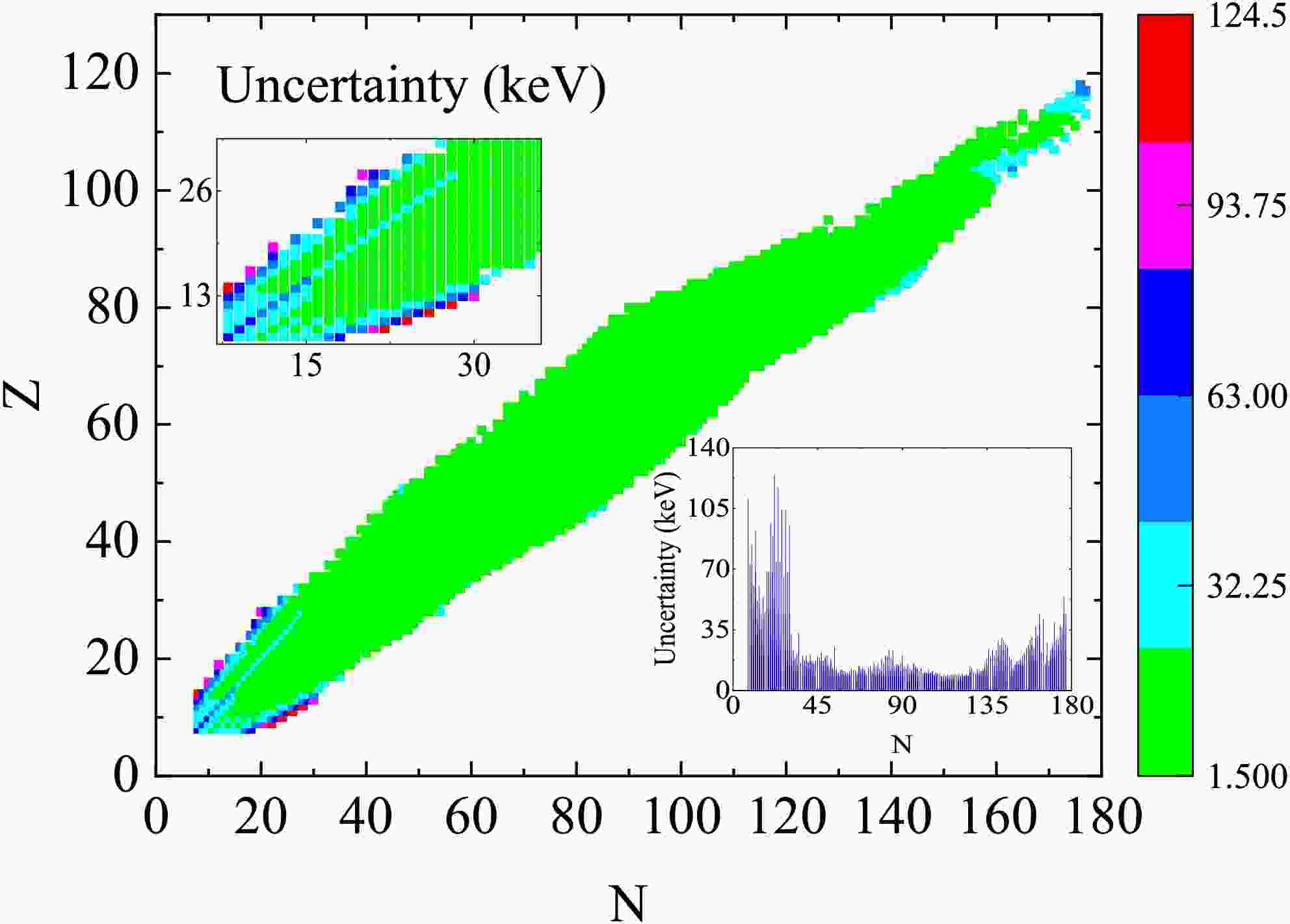
$ \nabla F=\left(\dfrac{\partial F}{\partial x_1},\dfrac{\partial F}{\partial x_2},\ldots,\dfrac{\partial F}{\partial x_n}\right)^T $ is the gradient vector.The error range of the predicted atomic mass values on the entire nuclide map calculated by Eq.(21) is from 1.996 to 124.469 keV, with an average value of 9.311 keV. The accuracy distribution characteristics of nuclear binding energy prediction were revealed through error analysis. As shown in the confidence heat map in Fig. 1, compared with the model error, the statistical error fluctuation of the predicted value of the combined energy is relatively small. In the low-mass number region (
$ A\leq50 $ ) and super-heavy core region ($ A> 210 $ ), the dispersion degree of the predicted value significantly increased ($ \Delta \sigma > 63 $ ) keV, while the medium-mass nuclide region ($ 50 < A \leq 210 $ ) presents a high confidence feature ($ \Delta \sigma < 32.25 $ ) keV.
Figure 1. (color online) Uncertainty of the predicted value of the binding energy.
To further analyze the error evolution law of the intermediate transition region, a relationship graph between the uncertainty of the predicted binding energy value and number of neutrons was constructed (embedded in lower right corner of Fig. 1). Quantitative analysis shows that the statistical error of the predicted binding energy value shows a trend of first decreasing and then increasing with increasing number of neutrons. Specifically, in the light nuclei region (
$ N<28 $ ), it reaches the peak ($ \Delta \sigma \approx 120 $ keV) and gradually converges to the stable state ($ \Delta \sigma \approx 20 $ keV) as the number of neutrons increases to the medium nuclei region ($ 28\leq N \leq 126 $ ). In the heavy nuclei region ($ N>126 $ ), a secondary increase phenomenon occurs again ($ \Delta \sigma \approx 40 $ keV). It is worth noting that the excellent performance of the higher-order terms of symmetry energy in the medium kernel region verifies the applicability of the BW3 formula in this region. -
$ \boldsymbol{x}=(x_{1},x_{2},\ldots,x_{n}) $ are random variables, the mathematical expectation of$ {\boldsymbol{\mu}}=({\mu}_{1},{\mu}_{2},\ldots,{\mu}_{n}) $ , and the covariance matrix is$ {\boldsymbol{\sum}} $ . Among them, the element$ \Sigma_{ij}=\mathrm{cov}(x_i,x_j) $ . Given a function$ \boldsymbol{y} = F ({x}) $ ,$ \boldsymbol{y} $ variance can use the covariance matrix representation of F.The first-order Taylor expansion of
$ F (\boldsymbol{x}) $ at$ {\boldsymbol{\mu}} $ is performed as follows:$ F(\boldsymbol{x})\approx F (\boldsymbol{x})+\sum\limits_{i=1}^n\left.\frac{\partial F}{\partial x_i}\right|_{{\boldsymbol{\mu}}}(x_i-\mu_i). $
(14) Here, higher-order minor terms (second-order and above) are ignored, and the uncertainty of the function is dominated by first-order linear terms.
Variance is defined by
$\begin{array}{*{20}{l}} \mathrm{Var}(\boldsymbol{y})=E\left[\left(F(\boldsymbol{x})-E[F(\boldsymbol{x})]\right)^2\right]. \end{array} $
(15) Substituting Eq.(14) gives
$ F(\boldsymbol{x})-E[F(\boldsymbol{x})]\approx\sum\limits_{i=1}^n\left.\frac{\partial F}{\partial x_i}\right|_{{\boldsymbol{\mu}}}(x_i-\mu_i). $
(16) Therefore, the variance is
$ \mathrm{Var}(\boldsymbol{y}) = \sum\limits_{i=1}^n\sum\limits_{j=1}^n\frac{\partial F}{\partial x_i}\frac{\partial F}{\partial x_j}E[(x_i-\mu_i)(x_j-\mu_j)]. $
(17) where
$ E[(x_i-\mu_i)(x_j-\mu_j)]=\mathrm{cov}(x_i,x_j)=\Sigma_{ij} $ .The final error transfer formula is
$ \mathrm{Var}({y}) =\sum_{i=1}^{N}\left(\frac{\partial F}{\partial x_{i}}\right)^{2}\mathrm{var}(x_{i})+2\sum_{i=1}^{N-1}\sum_{j=i+1}^{N}\frac{\partial F}{\partial x_{i}}\frac{\partial F}{\partial x_{j}}\mathrm{cov}(x_{i},x_{j}), $
which can also be expressed as
$ \sigma_{{y}}^{2} =\sum_{i=1}^{N}\left(\frac{\partial F}{\partial x_{i}}\right)^{2}\sigma_{x_{i}}^{2}+2\sum_{i=1}^{N-1}\sum_{j=i+1}^{N}\frac{\partial F}{\partial x_{i}}\frac{\partial F}{\partial x_{j}}\rho(x_{i},x_{j})\sigma_{x_{i}}\sigma_{x_{j}}, $
(18) where
$ \rho(x_{i},x_{j}) $ is the correlation coefficient between$ x_{i} $ and$ x_{j} $ , defined as$\begin{array}{*{20}{l}} \rho(x_i,x_j)=\mathrm{cov}(x_i,x_j)/\sigma_{x_i}\sigma_{x_j}. \end{array} $
(19) When
$ \rho(x_{i},x_{j})=0 $ , Eq. (18) becomes$ \sigma_{{y}}^{2}=\sum\limits_{i=1}^{N}\left(\frac{\partial F}{\partial x_{i}}\right)^{^2}\sigma_{x_{i}}^{^2}. $
(20) This is written in matrix form as
$\begin{array}{*{20}{l}} \mathrm{Var}(\boldsymbol{y}) = \nabla F^T \Sigma \nabla F, \end{array} $
(21) where
$ \nabla F=\left(\dfrac{\partial F}{\partial x_1},\dfrac{\partial F}{\partial x_2},\ldots,\dfrac{\partial F}{\partial x_n}\right)^T $ is the gradient vector.The error range of the predicted atomic mass values on the entire nuclide map calculated by Eq.(21) is from 1.996 to 124.469 keV, with an average value of 9.311 keV. The accuracy distribution characteristics of nuclear binding energy prediction were revealed through error analysis. As shown in the confidence heat map in Fig. 1, compared with the model error, the statistical error fluctuation of the predicted value of the combined energy is relatively small. In the low-mass number region (
$ A\leq50 $ ) and super-heavy core region ($ A> 210 $ ), the dispersion degree of the predicted value significantly increased ($ \Delta \sigma > 63 $ ) keV, while the medium-mass nuclide region ($ 50 < A \leq 210 $ ) presents a high confidence feature ($ \Delta \sigma < 32.25 $ ) keV.
Figure 1. (color online) Uncertainty of the predicted value of the binding energy.
To further analyze the error evolution law of the intermediate transition region, a relationship graph between the uncertainty of the predicted binding energy value and number of neutrons was constructed (embedded in lower right corner of Fig. 1). Quantitative analysis shows that the statistical error of the predicted binding energy value shows a trend of first decreasing and then increasing with increasing number of neutrons. Specifically, in the light nuclei region (
$ N<28 $ ), it reaches the peak ($ \Delta \sigma \approx 120 $ keV) and gradually converges to the stable state ($ \Delta \sigma \approx 20 $ keV) as the number of neutrons increases to the medium nuclei region ($ 28\leq N \leq 126 $ ). In the heavy nuclei region ($ N>126 $ ), a secondary increase phenomenon occurs again ($ \Delta \sigma \approx 40 $ keV). It is worth noting that the excellent performance of the higher-order terms of symmetry energy in the medium kernel region verifies the applicability of the BW3 formula in this region. -
$ {x}=(x_{1},x_{2},\ldots,x_{n}) $ as random variables, the mathematical expectation of$ {\boldsymbol{\mu}}=({\mu}_{1},{\mu}_{2},\ldots,{\mu}_{n}) $ , covariance matrix is$ {\boldsymbol{\sum}} $ . Among them, the element$ \Sigma_{ij}=\mathrm{cov}(x_i,x_j) $ . A given function$ {y} = F ({x}) $ ,$ {y} $ variance can use covariance matrix representation of F.Perform the first-order Taylor expansion of
$ F ({x}) $ at$ {\boldsymbol{\mu}} $ :$ F({x})\approx F ({x})+\sum\limits_{i=1}^n\left.\frac{\partial F}{\partial x_i}\right|_{{\boldsymbol{\mu}}}(x_i-\mu_i). $

(14) Here, higher-order minor terms (second-order and above) are ignored, and the uncertainty of the function is dominated by first-order linear terms.
Defined by variance
$\begin{array}{*{20}{l}} \mathrm{Var}({y})=E\left[\left(F({x})-E[F({x})]\right)^2\right]. \end{array} $

(15) Substitute Eq.(14)
$ F({x})-E[F({x})]\approx\sum\limits_{i=1}^n\left.\frac{\partial F}{\partial x_i}\right|_{{\boldsymbol{\mu}}}(x_i-\mu_i). $

(16) Therefore, the variance is
$ \mathrm{Var}({y}) = \sum\limits_{i=1}^n\sum\limits_{j=1}^n\frac{\partial F}{\partial x_i}\frac{\partial F}{\partial x_j}E[(x_i-\mu_i)(x_j-\mu_j)]. $

(17) where
$ E[(x_i-\mu_i)(x_j-\mu_j)]=\mathrm{cov}(x_i,x_j)=\Sigma_{ij} $ .The final error transfer formula is
$ \mathrm{Var}({y}) =\sum_{i=1}^{N}\left(\frac{\partial F}{\partial x_{i}}\right)^{2}\mathrm{var}(x_{i})+2\sum_{i=1}^{N-1}\sum_{j=i+1}^{N}\frac{\partial F}{\partial x_{i}}\frac{\partial F}{\partial x_{j}}\mathrm{cov}(x_{i},x_{j}), $

or expressed as
$ \sigma_{{y}}^{2} =\sum_{i=1}^{N}\left(\frac{\partial F}{\partial x_{i}}\right)^{2}\sigma_{x_{i}}^{2}+2\sum_{i=1}^{N-1}\sum_{j=i+1}^{N}\frac{\partial F}{\partial x_{i}}\frac{\partial F}{\partial x_{j}}\rho(x_{i},x_{j})\sigma_{x_{i}}\sigma_{x_{j}}, $

(18) where
$ \rho(x_{i},x_{j}) $ is the correlation coefficient between$ x_{i} $ and$ x_{j} $ , defined as$\begin{array}{*{20}{l}} \rho(x_i,x_j)=\mathrm{cov}(x_i,x_j)/\sigma_{x_i}\sigma_{x_j}. \end{array} $

(19) When
$ \rho(x_{i},x_{j})=0 $ , the Eq. (18) becomes$ \sigma_{{y}}^{2}=\sum\limits_{i=1}^{N}\left(\frac{\partial F}{\partial x_{i}}\right)^{^2}\sigma_{x_{i}}^{^2}. $

(20) It is written in matrix form as
$\begin{array}{*{20}{l}} \mathrm{Var}({y}) = \nabla F^T \Sigma \nabla F, \end{array} $

(21) where
$ \nabla F=\left(\dfrac{\partial F}{\partial x_1},\dfrac{\partial F}{\partial x_2},\ldots,\dfrac{\partial F}{\partial x_n}\right)^T $ is the gradient vector.The error range of the predicted atomic mass values on the entire nuclide map calculated by the Eq.(21) is from 1.996 to 124.469 keV, with an average value of 9.311 keV. The accuracy distribution characteristics of nuclear binding energy prediction were revealed through error analysis. As shown in the confidence heat map Fig. 1, compared with the model error, the statistical error fluctuation of the predicted value of the combined energy is quite small. In the low-mass number region (
$ A\leq50 $ ) and the super-heavy core region ($ A> 210 $ ), the dispersion degree of the predicted value has significantly increased ($ \Delta \sigma > 63 $ ) keV, while the medium-mass nuclide region ($ 50 < A \leq 210 $ ) presents a high confidence feature ($ \Delta \sigma < 32.25 $ ) keV.
Figure 1. (color online) The uncertainty of the predicted value of the binding energy.
To further analyze the error evolution law of the intermediate transition region, a relationship graph between the uncertainty of the predicted binding energy value and the number of neutrons was constructed (embedded Fig. 1 at the lower right corner). Quantitative analysis shows that the statistical error of the predicted binding energy value shows a trend of first decreasing and then increasing with the increase of the number of neutrons. Specifically, in the light nuclei region (
$ N<28 $ ) it reaches the peak ($ \Delta \sigma \approx 120 $ keV), and gradually converges to the stable state ($ \Delta \sigma \approx 20 $ keV) as the number of neutrons increases to the medium nuclei region ($ 28\leq N \leq 126 $ ). And in the heavy nuclei region ($ N>126 $ ) a secondary increase phenomenon occurred again ($ \Delta \sigma \approx 40 $ keV). It is worth noting that the excellent performance of the higher-order terms of symmetry energy in the medium kernel region verifies the applicability of the BW3 formula in this region. -
This study employed nuclear mass data from the AME2020 database to generate normally distributed random nuclear mass values via the Monte Carlo method (5, 000 samples), subsequently fitting and deriving 5, 000 sets of optimized BW3 parameters while quantifying their standard deviations and Pearson correlation coefficients. Correlation information can be extracted from the final parameter distributions.
The visualization scheme in Fig. 2 systematically reveals linear correlation patterns among parameters. This figure implements a partitioned visualization strategy: the upper triangular section employs two-dimensional kernel density estimation to demonstrate association intensity, where elliptical distributions indicate strong linear correlations and circular patterns denote weak/no significant associations; the lower triangular section utilizes graduated color-scale heatmaps to quantify Pearson correlation coefficients between BW3 parameter pairs, with the chromatic spectrum spanning deep red (
$ r=-1 $ ) to deep blue ($ r=+1 $ ).
Figure 2. (color online) Matrix heat map and two-dimensional histogram of BW3 model parameters obtained by bootstrapping method. The color code of the two-dimensional histogram is a heat map. The total number of parameters involved in each graph is fixed at T=5000.
It can be seen from Fig. 2 that there is significant collinearity among the volume, surface, Coulomb, and curvature terms. The model represents the binding energy of atomic nuclei as a power series expansion of the reciprocal of the nuclear radius (
$ 1/R $ ). Because the relationship between the nuclear radius R and number of nucleons A is$ R \propto A^{1/3} $ , these terms are actually functions of different powers of$ A^{1/3} $ (such as the volume term$ \propto A $ , surface term$ \propto A^{2/3} $ , Coulomb term$ \propto Z^2/A^{1/3} $ , and curvature term$ \propto A^{1/3} $ ). The shell correction term based on the number of valence nucleons presents a binary coupling structure, and the relationship among its parameters is significant ($ r=-0.92 $ ). This indicates that the parameters describing the shell effect are not independent. The change of one parameter can be offset by the change of another parameter. This means that the parametric form of shell correction terms must be optimized to reduce this redundancy. The paired items show statistical independence characteristics in the entire parameter system. Its independence indicates that the pairing term provides unique physical information for the nuclear mass formula that cannot be replaced by any other term.The higher-order terms of symmetry energy and the surface symmetry terms show the strongest covariation trend (
$ r=-0.43 $ ). This means that when fitting nuclear mass data, it is very difficult to separate the surface symmetry effect from the higher-order correction effect of symmetry energy. This directly affects the coefficients for precisely extracting the higher-order terms of symmetric energy from the atomic nucleus mass. The above analysis provides a clear direction for the further development and optimization of the droplet model: reduce or eliminate the collinearity between the core droplet terms (volume, surface, coulomb, and curvature) and the symmetry energy terms, and explore alternative mathematical expressions that do not rely entirely on the expansion of$ 1/R $ power series. -
This study employs nuclear mass data from the AME2020 database to generate normally distributed random nuclear mass values via Monte Carlo method (5,000 samples), subsequently fitting and deriving 5,000 sets of optimized BW3 parameters while quantifying their standard deviations and Pearson correlation coefficients. Correlation information can be extracted from the final parameter distributions.
The visualization scheme in Fig. 2 systematically reveals linear correlation patterns among parameters. This figure implements a partitioned visualization strategy: the upper triangular section employs two-dimensional kernel density estimation to demonstrate association intensity, where elliptical distributions indicate strong linear correlations and circular patterns denote weak/no significant associations; the lower triangular section utilizes graduated color-scale heatmaps to quantify Pearson correlation coefficients between BW3 parameter pairs, with the chromatic spectrum spanning deep red (
$ r=-1 $ ) to deep blue ($ r=+1 $ ).
Figure 2. (color online) Matrix heat map and two-dimensional histogram of BW3 model parameters obtained by bootstrapping method. The color code of a two-dimensional histogram is a heat map. The total number of parameters involved in each graph is fixed at T=5000.
It can be known from Fig. 2 that there is significant collinearity among the volume term, surface term, Coulomb term and curvature term. The model represents the binding energy of atomic nuclei as a power series expansion of the reciprocal of the nuclear radius (
$ 1/R $ ). Since the relationship between the nuclear radius R and the number of nucleons A is$ R \propto A^{1/3} $ , these terms are actually functions of different powers of$ A^{1/3} $ (such as the volume term$ \propto A $ , the surface term$ \propto A^{2/3} $ , the coulomb term$ \propto Z^2/A^{1/3} $ , and the curvature term$ \propto A^{1/3} $ ). The shell correction term based on the number of valence nucleons presents a binary coupling structure, and the relationship among its parameters is significant ($ r=-0.92 $ ). This indicates that the parameters describing the shell effect are not independent. The change of one parameter can be offset by the change of another parameter. This means that the parametric form of shell correction terms needs to be optimized to reduce this redundancy. The paired items show statistical independence characteristics in the entire parameter system. Its independence indicates that the pairing term provides unique physical information for the nuclear mass formula that cannot be replaced by any other term.
Figure 4. (color online) Comparison of binding energy prediction results before and after BW3 formula coefficients update.
The higher-order terms of symmetry energy and the surface symmetry terms show the strongest covariation trend (
$ r=-0.43 $ ). This means that when fitting nuclear mass data, it is very difficult to separate the surface symmetry effect from the higher-order correction effect of symmetry energy. This directly affects the coefficients for precisely extracting the higher-order terms of symmetric energy from the atomic nucleus mass. The above analysis provides a clear direction for the further development and optimization of the droplet model. Reduce or eliminate the collinearity between the core droplet terms (volume, surface, coulomb, curvature) and the symmetry energy terms. Explore alternative mathematical expressions that do not rely entirely on the expansion of$ 1/R $ power series. -
The optimization performance of the model can be revealed through the three-dimensional error distribution map (Fig. 3). In the figure, the blue dots represent the calculation results after parameter optimization, while the black dots represent the benchmark data of the original model. Analysis shows that the error distribution characteristics of the modified model converge significantly toward the zero-value reference plane, indicating that the root mean square error between the calculated and experimental binding energy values presents a systematic reduction. The error surface presents a parabolic shape that rises first and then falls. This shows significant changes in the region with a low number of nucleons and gradually stabilizes as the number of nucleons increases.

Figure 3. (color online) 3D comparison of prediction results before and after updating of BW3 formula coefficients.
To explore which types of nuclei the mass model has a greater effect on after updating the coefficients, the predictive efficacy of the BW3 formula parameter optimization was systematically evaluated for the binding energies of different types of atomic nuclei. Figure 4 shows the comparative analysis framework before and after the model correction, including the nuclide distribution and residual mapping diagrams. The horizontal axis represents the number of neutrons and corresponding residual distribution range, and the vertical axis describes the number of protons and the corresponding residual range. The residual distribution graph at the top shows the relationship between the residual and number of neutrons, and that on the right shows the relationship between the residual and number of protons.
Figure 4. (color online) Comparison of binding energy prediction results before and after BW3 formula coefficient update.
The statistical evaluation based on the least square method shows that the parameter optimization significantly improves the calculation accuracy of the nuclide binding energy. The residual distribution characteristics show that the error convergence in the neutron-rich nucleus region is better than that in the neutron-deficient nucleus region, which is closely related to the core-shell filling effect on the calculation accuracy of the binding energy of the model. The improvement in the proton droplet line region was more significant. The root mean square error was optimized from 2.89 MeV to 1.92 MeV, with a reduction of 33.6%. In the neutron drop line region, the root mean square error decreased from 2.42 MeV to 1.89 MeV, and the relative optimization amplitude reached 21.9%. To further investigate the impact of parameter uncertainties on mass difference, the single neutron separation energies are compared with data in neutron-rich nuclei. As shown in Fig. 5, the calculations reproduce experimental values well in the medium and heavy nuclear regions, except for
$ ^{113}_{40} $ Zr$ ^{73} $ . The difference is large before$ Z < 20 $ or$ A < 56 $ . The update of formula coefficients makes a slight improvement in single neutron separation energies. For example, the value for$ ^{165}_{61} $ Pm$ ^{104} $ changes from 4.866 to 4.863 MeV (datum is 4.384 MeV). Such little improvement can not be distinguished in Fig. 5.
Figure 5. (color online) Single neutron separation energies in neutron-rich nuclei. Label A refers to nuclear mass. Results Th1 (Th2) are before (after) BW3 formula coefficient update.
-
The optimization performance of the model can be revealed through the three-dimensional error distribution map (Fig. 3). In the figure, the blue dots represent the calculation results after parameter optimization, while the black dots represent the benchmark data of the original model. Analysis shows that the error distribution characteristics of the modified model converge significantly toward the zero-value reference plane, indicating that the root mean square error between the calculated and experimental binding energy values presents a systematic reduction. The error surface presents a parabolic shape that rises first and then falls. This shows significant changes in the region with a low number of nucleons and gradually stabilizes as the number of nucleons increases.
Figure 3. (color online) 3D comparison of prediction results before and after updating of BW3 formula coefficients.
To explore which types of nuclei the mass model has a greater effect on after updating the coefficients, the predictive efficacy of the BW3 formula parameter optimization was systematically evaluated for the binding energies of different types of atomic nuclei. Figure 4 shows the comparative analysis framework before and after the model correction, including the nuclide distribution and residual mapping diagrams. The horizontal axis represents the number of neutrons and corresponding residual distribution range, and the vertical axis describes the number of protons and the corresponding residual range. The residual distribution graph at the top shows the relationship between the residual and number of neutrons, and that on the right shows the relationship between the residual and number of protons.
Figure 4. (color online) Comparison of binding energy prediction results before and after BW3 formula coefficient update.
The statistical evaluation based on the least square method shows that the parameter optimization significantly improves the calculation accuracy of the nuclide binding energy. The residual distribution characteristics show that the error convergence in the neutron-rich nucleus region is better than that in the neutron-deficient nucleus region, which is closely related to the core-shell filling effect on the calculation accuracy of the binding energy of the model. The improvement in the proton droplet line region was more significant. The root mean square error was optimized from 2.89 MeV to 1.92 MeV, with a reduction of 33.6%. In the neutron drop line region, the root mean square error decreased from 2.42 MeV to 1.89 MeV, and the relative optimization amplitude reached 21.9%. To further investigate the impact of parameter uncertainties on mass difference, the single neutron separation energies are compared with data in neutron-rich nuclei. As shown in Fig. 5, the calculations reproduce experimental values well in the medium and heavy nuclear regions, except for
$ ^{113}_{40} $ Zr$ ^{73} $ . The difference is large before$ Z < 20 $ or$ A < 56 $ . The update of formula coefficients makes a slight improvement in single neutron separation energies. For example, the value for$ ^{165}_{61} $ Pm$ ^{104} $ changes from 4.866 to 4.863 MeV (datum is 4.384 MeV). Such little improvement can not be distinguished in Fig. 5.
Figure 5. (color online) Single neutron separation energies in neutron-rich nuclei. Label A refers to nuclear mass. Results Th1 (Th2) are before (after) BW3 formula coefficient update.
-
The optimization performance of the model is revealed through the three-dimensional error distribution map (Fig. 3). In the figure, the blue spheres represent the calculation results after parameter optimization, while the black spheres represent the benchmark data of the original model. Analysis shows that the error distribution characteristics of the modified model converge significantly towards the zero-value reference plane, indicating that the root mean square error between the calculated binding energy value and the experimental value after optimization presents a systematic reduction. The error surface presents a parabolic shape that rises first and then falls. It shows significant changes in the region with a low number of nucleons and gradually stabilizes as the number of nucleons increases.
Figure 3. (color online) 3D comparison of prediction results before and after updating of BW3 formula coefficients.
In order to explore which types of nuclei the mass model after updating the coefficients has a greater effect on, the predictive efficacy of the BW3 formula parameter optimization for the binding energy of different types of atomic nuclei was systematically evaluated. Figure 5 shows the comparative analysis framework before and after the model correction, including the nuclide distribution and residual mapping diagrams. The horizontal axis represents the number of neutrons and the corresponding residual distribution range, the vertical axis describes the number of protons and the corresponding residual range, the residual distribution graph at the top shows the relationship between the residual and the number of neutrons, and the one on the right shows the relationship between the residual and the number of protons.
Figure 5. (color online) The single neutron separation energies in Neutron-rich nuclei.Label A means nuclear mass. Results Th1 (Th2) are before (after) BW3 formula coefficients update.
The statistical evaluation based on the least square method shows that the parameter optimization significantly improves the calculation accuracy of the nuclide binding energy. The residual distribution characteristics show that the error convergence in the neutron-rich nucleus region is better than that in the neutron-deficient nucleus region, which is closely related to the core-shell filling effect on the calculation accuracy of the binding energy of the model. The improvement in the proton droplet line region was more significant. The root mean square error was optimized from 2.89 MeV to 1.92 MeV, with a reduction of 33.6%. In the neutron drop line region, the root mean square error decreases from 2.42 MeV to 1.89 MeV, and the relative optimization amplitude reaches 21.9%. For further investigating the impact of parameter uncertainties on mass difference, the single neutron separation energies are compared with data in neutron-rich nuclei. As shown in Fig. 5, the calculations reproduce experimental value well in medium and heavy nuclear region, except
$ ^{113}_{40} $ Zr$ ^{73} $ . The difference is some large before$ Z < 20 $ or$ A < 56 $ . The update of formula coefficients make a slight improvement in single neutron separation energies. For example, the value in$ ^{165}_{61} $ Pm$ ^{104} $ is from 4.866 to 4.863 MeV (datum is 4.384 MeV). Such little improvement can not be distinguished in Fig. 5. -
In summary, we studied the ground state properties and predictive power of atomic nuclei by using the improved nuclear mass formula. Combining least squares fitting and Monte Carlo sampling, 5,000 traversal calculations were conducted on the 12-dimensional parameter space to re-fit the parameters of the BW3 mass formula. Our main conclusions are as follows:
(1) The root mean square error of the improved BW3 mass formula was reduced to 1.66 MeV, which is 10.7% lower than before.
(2) In the proton droplet line region, the root mean square error was optimized from 2.89 MeV to 1.92 MeV, with a reduction of 33.6%. In the neutron droplet line region, the root mean square error decreased from 2.42 MeV to 1.89 MeV, and the relative optimization amplitude reached 21.9%.
(3) There is significant collinearity among the volume, surface, Coulomb, and curvature terms. The shell correction term based on the number of valence nucleons presents a binary coupling structure, and there is a significant correlation among its parameters. The curvature term shows a weak correlation feature with the paired term but has a strong correlation with the remaining terms. The paired items show statistical independence in the entire parameter system. The higher-order terms of symmetry energy show a significant correlation with the surface symmetry terms.
(4) The error situation of theoretical binding energy was studied using error transfer theory. The error range of the predicted atomic mass value on the entire nuclide map is from 1.996 to 124.469 keV, with an average value of 9.311 keV. The error shows a trend of first decreasing and then increasing with increasing number of neutrons.
Our results are in good agreement with some experimental and theoretical studies. This study demonstrates good performance in the neutron-rich mass region, which is useful for rapid neutron capture in nuclear astrophysics.
-
In summary, we studied the ground state properties and predictive power of atomic nuclei by using the improved nuclear mass formula. Combining least squares fitting and Monte Carlo sampling, 5,000 traversal calculations were conducted on the 12-dimensional parameter space to re-fit the parameters of the BW3 mass formula. Our main conclusions are:
(1) The root mean square error of the improved BW3 mass formula was reduced to 1.66 MeV, which was 10.7% lower than before.
(2) In the proton droplet line region, The root mean square error was optimized from 2.89 MeV to 1.92 MeV, with a reduction of 33.6%. In the neutron droplet line region, the root mean square error decreased from 2.42 MeV to 1.89 MeV, and the relative optimization amplitude reached 21.9%.
(3) There is significant collinearity among the volume term, surface term, Coulomb term and curvature term. The shell correction term based on the number of valence nucleons presents a binary coupling structure, and there is a significant correlation among its parameters. The curvature term shows a weak correlation feature with the paired term, but has a strong correlation with the remaining terms. The paired items show statistical independence in the entire parameter system. The higher-order terms of symmetry energy show a significant correlation with the surface symmetry terms.
(4) The error situation of theoretical binding energy was studied by using the error transfer theory. The error range of the predicted atomic mass value on the entire nuclide map is from 1.996 to 124.469 keV, with an average value of 9.311 keV. The error shows a trend of first decreasing and then increasing with the increase of the number of neutrons.
Our results are in good agreement with some experimental and theoretical studies. This study demonstrates good performance in the neutron-rich mass region, which is useful for rapid neutron capture in nuclear astrophysics.
-
In summary, we studied the ground state properties and predictive power of atomic nuclei by using the improved nuclear mass formula. Combining least squares fitting and Monte Carlo sampling, 5,000 traversal calculations were conducted on the 12-dimensional parameter space to re-fit the parameters of the BW3 mass formula. Our main conclusions are as follows:
(1) The root mean square error of the improved BW3 mass formula was reduced to 1.66 MeV, which is 10.7% lower than before.
(2) In the proton droplet line region, the root mean square error was optimized from 2.89 MeV to 1.92 MeV, with a reduction of 33.6%. In the neutron droplet line region, the root mean square error decreased from 2.42 MeV to 1.89 MeV, and the relative optimization amplitude reached 21.9%.
(3) There is significant collinearity among the volume, surface, Coulomb, and curvature terms. The shell correction term based on the number of valence nucleons presents a binary coupling structure, and there is a significant correlation among its parameters. The curvature term shows a weak correlation feature with the paired term but has a strong correlation with the remaining terms. The paired items show statistical independence in the entire parameter system. The higher-order terms of symmetry energy show a significant correlation with the surface symmetry terms.
(4) The error situation of theoretical binding energy was studied using error transfer theory. The error range of the predicted atomic mass value on the entire nuclide map is from 1.996 to 124.469 keV, with an average value of 9.311 keV. The error shows a trend of first decreasing and then increasing with increasing number of neutrons.
Our results are in good agreement with some experimental and theoretical studies. This study demonstrates good performance in the neutron-rich mass region, which is useful for rapid neutron capture in nuclear astrophysics.
Uncertainty analysis of the nuclear liquid drop model
- Received Date: 2025-08-16
- Available Online: 2026-02-15
Abstract: This study performed a statistical analysis of the correlation and uncertainty of parameters in the classical liquid drop mass formula (namely BW3 type) via regression, along with the theoretical impact of error propagation. Within the improved BW3 formula, the total deviation between evaluation and experiment can be reduced to 1.66 MeV, involving a reduction from 2.89 (2.42) MeV to 1.92 (1.89) MeV in the proton(neutron)-dripline region. Ridge regression validation verified this total deviation as the optimal point in the present mass model. Through trend coefficients and Pearson linear-correlation analysis, obvious collinearity was identified between volume, surface, Coulomb, and curvature terms, with notable correlation among high-order symmetry energy and surface symmetry terms. The theoretical derivation of the distribution of binding energy error was then achieved through error propagation analysis. Across the nuclide chart, the error uncertainty of mass predictions varies from 1.996 to 124.469 keV, demonstrating a convex trend of the initial decrease of evaluation error followed by an increase versus the neutron number.


 DownLoad: