Study of excited D and D_s mesons in a relativized quark model

Quantum Chromodynamics (QCD) is an experimentally well established theory of the strong interaction of quarks and gluons. However, describing the rich spectrum of hadrons from first principles is still challenging owing to the non-perturbative nature of QCD at low energy. Considering this difficulty, many models and theoretical approaches have been adopted to calculate hadron properties. The quark model, where applicable, is considered to be a convenient tool. According to the quark model, a conventional meson is a bound state of a quark and an antiquark. The model predicts that a meson can have only certain values of $ J^{PC} $. The mesons with $ J^{PC} $ differing from quark-model values are called exotic mesons. In 1993, an exotic meson in the light quark sector having $ J^{PC} $ = 1^–+, was observed by the VES Collaboration [1]. Many exotic mesons have been observed since. Theoretically, exotic mesons could be glueball, tetra quark, or hybrid mesons. It is noted that the $ J^{PC} $ of these mesons can be allowed or forbidden by the quark model. Lattice QCD successfully describes these exotics [2−6]. Phenomenological models also provide a good description of the properties of exotic mesons [7−14]. In open flavor mesons where quarks and antiquarks have different flavors, C parity no longer remains a good quantum number. In this case, states are identified by their $ J^P $ values only. The states having the same $ J^P $ value are mixed. Indeed, all $ J^P $ states are mixed except 0⁺ and 0^-. Mixing is either spin mixing or S-D mixing. This mixing will be discussed in detail in Section III. Incorporating mixing, where needed, we study the properties of hybrid as well as conventional mesons in the open charm meson sector, specifically charmed (D) mesons and charmed strange ($ D_s $) mesons.

The gluonic field plays a dominant role in binding quarks. In conventional mesons, the gluonic field is in the ground state and in the excited state for hybrid mesons. We are particularly interested in studying the $ \Pi_u $ state, where the gluonic field is in its first excited state. We use the leading Born-Oppenheimer approximation (LBO) for calculating the spectrum of hybrid mesons. In this approximation, a hybrid meson is treated as a diatomic molecule in which quarks and gluons are considered as nuclei and electrons, respectively. There are two steps involved in applying LBO approximation. In the first step, the static potential energy of gluons is determined by treating quarks and antiquarks as spatially fixed, and in the second step, the motion of quarks is restored using this potential in the Schrödinger wave equation. The parity of the hybrid meson is $ \varepsilon(-1)^{L+\Lambda+1} $, where $ \Lambda $ is the magnitude of the projection of total angular momentum of the gluonic field onto the molecular axis. For the $ \Pi_u $ potential, where the gluonic field is in its first excited state, $ \Lambda=1 $ and $ \varepsilon=\pm1 $ [2, 3].

The D and $ D_s $ meson domain has immense amounts of experimental data. The first two charmed mesons ($ D^0 $ and $ D^\pm $) were discovered by the Mark I experiments in 1976 [15, 16]. Their $ J^P $ is 0^–. $ D^0 $ and $ D^\pm $ have masses $ 1864.83\pm 0.05 $ MeV and $ 1869.58\pm0.09 $ MeV, respectively. One year later, the first charmed strange meson ($ D_s^{\pm} $) of $ J^P $ = 0^–, was observed by the DASP Collaboration [17]. The mass of $ D_s^{\pm} $ is 1968.34 ± 0.07 MeV [18]. In the same experiment, $ D_s^{*\pm} $ meson was also discovered to have a mass of $ 2112.1\pm0.4 $ MeV and $ J^P=1^- $. At present, data for more than twenty well recognized states have been collected. Information of their masses, $ J^P $ values, and dozens of their decay modes are available in the Particle Data Group (PDG) listings [18]. In parallel, extensive work has been done to calculate their masses and other properties. Using Schrödinger-like wave equations in relativistic dynamics, the spectrum and wave functions of D and $ D_s $ mesons were calculated in Refs. [19−22]. In Ref. [20], strong and radiative transitions were reported. Refs. [23, 24] implemented the Dirac formalism to calculate the spectrum, radiative transitions, decay constant, and leptonic decay width of the $ D_s $ and D meson systems, respectively. In Ref. [25], the spectrum and wave functions of D and $ D_s $ mesons were obtained using the Bethe-Salpeter equation. Ref. [26] computed the spectrum of the heavy-light meson with the aid of a QCD motivated relativistic quark model. They investigated Regge trajectories as well. Using the Dirac Hamiltonian, Ref. [27] computed the mass spectra, wave functions, and hadronic transitions of heavy-light mesons. They also added leading order corrections in $ 1/m_{c,b} $. In Ref. [28], the spectrum of D and $ D_s $ mesons was calculated using Wilson twisted mass lattice QCD. Refs. [21, 22] discretized the relativistic wave equation using the Cornell potential (Coulomb plus linear potential). After calculating the masses and wavefunctions of mesons by diagonalizing the resulting Hamiltonian matrix, the spin dependent part of the Hamiltonian is added perturbatively because states with different principal quantum numbers can also have the same $ J^P $. Thus, several principal quantum numbers collectively contribute to one mixed state (either spin mixed or S-D mixed). In Refs. [21, 22], the contribution of two to three principal quantum numbers was included to describe a mixed state. Another limitation of their work is that the perturbative effects of spin dependent potential are included in the masses but not in the wave function. This is understandable because first order perturbative correction to wave functions involves a sum over all possible internal states, which is extremely difficult to calculate. We adopted the same approach to solve the relativistic wave equation as in Refs. [21, 22], with improvements that address the limitations of the approach used in Refs. [21, 22]. Instead of including the spin dependent part of the Hamiltonian perturbatively, we also include spin dependent terms in the Hamiltonian matrix. For this purpose, we developed a system of coupled equations for mixed states. As we are solving the coupled equations nonperturbatively, we are not restricted to including the contribution of only two to three principal quantum numbers to describe a mixed state. Two charmed strange mesons named $ D^*_{s0}(2317)^{\pm} $ and $ D_{s1}(2460)^{\pm} $ attract special attention as the observed values of their masses are much lower than the quark model predictions. Attempts have been made to describe them through alternative models [29−32]. Extensive work has been carried out in the literature to determine the nature of these mesons. In some studies [33, 34], these states are interpreted as tetraquarks, while in others, $ D^*_{s0}(2317)^{\pm} $ and $ D_{s1}(2460)^{\pm} $ are regarded as $ DK $ and $ DK^{*} $ molecule states, respectively [35, 36]. In Refs. [37, 38], these states are well described by including coupled-channel effects. Ref. [37] suggests that these states are the mixtures of bare $ c\bar{s} $ core and $ D^{(*)}K $ component. In Refs. [20−22, 39], these states have been studied as conventional mesons. The exact structure of these particles is still an open question in hadron physics.

In this study, we calculate masses, wave functions, and radiative transitions of conventional as well as hybrid D and $ D_s $ mesons, incorporating spin and S-D mixing effects on spectrum and wave functions. Unlike previous studies, we solve the Schrödinger-type equation using the full semi-relativistic Hamiltonian, including the spin-dependent part. This approach allows us to study both spin effects and S-D mixing without relying on perturbation theory.

This paper is structured as follows: In Section II, we describe our potential model for conventional and hybrid mesons. We use an extended version of the famous GI model. For the hybrid mesons, we add the potential model of gluonic excitation, which we have suggested in a previous study. In this study, we improve the parameter fitting of our proposed gluonic excited potential model by considering the latest lattice data [6]. In Section III, the phenomena of state mixing are examined. We distinguish two categories of mixed states. We also discuss the effects of the spin dependent part of the potential model on the spectrum. In Section IV, we describe our relativistic wave equation. We explicitly describe how we calculate masses and wave functions of mesons using a relativistic wave equation. State mixing effects in the Hamiltonian matrix are discussed as well. Radiative transitions of charmed and charmed strange mesons are reviewed in Section V. In the last section, we report our results and concluding remarks based on our calculations.

Phenomenological potential models are successful in describing various properties of heavy quark mesons, particularly mass [19−25, 40−43]. Among the suggested models, the GI model [19] is the most well-known. In this study, we have used it with some modifications.

The conventional D and $ D_s $ mesons are bound states of heavy quarks (Q = c) and a light antiquarks ($ \bar{q} = \bar{u} $/$ \bar{d} $, $ \bar{s} $), respectively. The potential model of a conventional meson $ V_{Q\bar{q}}(r) $ is

where r is the inter-quark distance. The first term of the potential model, called the Coulomb term, is calculated by one gluon exchange diagram in perturbation theory. It determines the behavior of potentials at small distances. $ \alpha_s(r) $ is a strong running coupling constant of QCD. Its parameterization is given by [19]

where $ \alpha_k^{\;,}s $ and $ \gamma_k^{\;,}s $ are free parameters. In this study, we take $ \gamma_1 $ = $ \dfrac{1}{2} $, $ \gamma_2 $ = $ \dfrac{\sqrt{10}}{2}\; $, and $ \gamma_3 $ = $ \dfrac{\sqrt{1000}}{2}\; $, as in Ref. [19]. With this choice of $ \gamma $'s, $ \alpha_2 $ and $ \alpha_3 $ control the shape of running coupling at small distances (large $ Q^2 $), where it is already fixed by pQCD. This allows us to fix $ \alpha_2=0.16 $ and $ \alpha_3=0.20 $ through fitting with 2-loop running coupling. Consequently, the parameter $ \alpha_1 $ (or $ \alpha_s^c\equiv\alpha_1+\alpha_2+\alpha_3 $), which controls the shape of the running coupling in the infrared region, is treated as a free parameter that is fixed via spectroscopy [19, 44]. Figure 1 shows the comparisons of $ \alpha_s(Q^2) $ of the parametrized model with the results obtained using our fitted $ \alpha_s^c=0.24 $ and pQCD 2-loop result.

Figure 1.  Strong running coupling constant in the momentum space. The solid curve represents data from the parametrized model and the dotted curve represents data from QCD perturbative calculations up to two loop corrections.

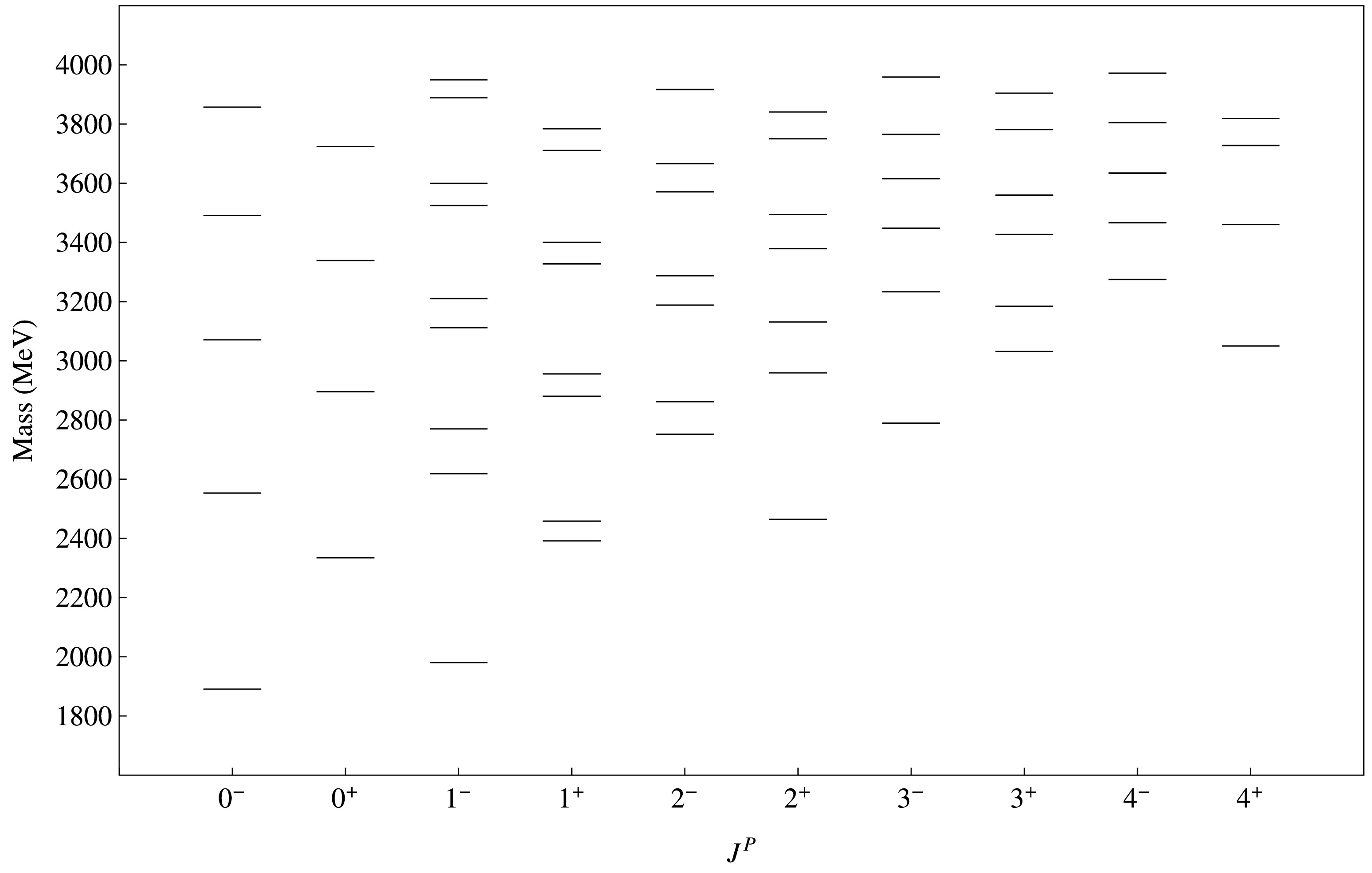
Figure 2.  Conventional charmed meson spectrum.

The second term of the potential is the confinement term, which dominates at large distances. The parameter b represents the string tension and is determined by fitting the spectrum. The third term, c, is also treated as a free parameter in the potential model. The last part of the potential model, the spin dependent term $V_{\text{spin-dep}}(r)$, is defined as follows:

where $V_{\rm hyp}(r)$ is the spin-spin contact hyperfine interaction [43]. It is defined as

where $ \langle {{\bf{S}}_{\bf{Q}}\cdot{\bf{S}}_{\bar{{\bf{q}}}}} \rangle $ = $ \dfrac{S(S+1)}{2}-\dfrac{3}{4} $. In Ref. [19], the parameter $ \sigma $ is

Numerical values of parameters $ \sigma_0 $ and $ s_0 $ are determined by fitting the spectrum. In Eq. (3), $ V_T(r) $ is the tensor term defined as

where T is the tensor operator:

The tensor operator has nonvanishing matrix elements only between $ L>0 $ and spin triplet states. The diagonal Hamiltonian matrix entries of the tensor operator are [43]

To study S-D mixed states, we require the off diagonal matrix element of the tensor operator

where $ L^{'} = L $ + 2. In Eq. (3), $V_{\rm so}(r)$ is the spin-orbit interaction term. It consists of two parts, such that

Here,$V_{\rm sov}(r)$ is a spin-orbit vector:

and $V_{\rm sos}(r)$ is the spin-orbit scalar part of the spin-orbit interaction term

For diagonal Hamiltonian matrices, $ \langle {{\bf{L}}\cdot{\bf{S}}_{\bf{Q}}} \rangle $ = $ \langle {{\bf{L}}\cdot{\bf{S}}_{\bar{\bf{q}}}} \rangle $ = $ \dfrac{\langle {{\bf{L}}\cdot{\bf{S}}} \rangle}{2} $, where $ \langle {{\bf{L}}\cdot{\bf{S}}} \rangle $ is

To study spin mixed states, we require the following matrix element of the $ \langle {{\bf{L}}.{\bf{S}}_{\bf{Q}}} \rangle $ and $ \langle {{\bf{L}}.{\bf{S}}_{\bar{\bf{q}}}} \rangle $ operators:

The form of the spin dependent part of the potential model is extracted from leading order perturbation theory in the non-relativistic approximation. However, this is not a good approximation, particularly for light quarks in heavy light mesons. Owing to the presence of a light quark in charmed and charmed strange mesons, it is essential to incorporate relativistic effects. These effects modify the potential in two distinct ways [19]: First, the quark antiquark separation (r) becomes smeared over a distance on the order of the inverse quark mass. By introducing the smearing function [19], smearing over $ 1/r^3 $ terms in the spin dependent part of the potential model is incorporated. Smearing also eliminates instability in the solution of the relativistic wave equation, which occurs at short distances due to the $ 1/r^3 $ term in the spin dependent potential model and makes the solution stable even at short distances. The second way to incorporate relativistic effects is to make the potential model momentum dependent. Momentum dependence in the spin dependent term can be effectively incorporated by introducing multiple constant factors. This modification is applied only to the light quark, as the momentum terms for the heavy quark effectively drop out. As momentum dependence modifies each spin interaction term differently, we introduce multiple constants ($ \epsilon_i $), each specific to a particular interaction. Here, i = 1, 2, 3, and 4 correspond to the hyperfine term, tensor term, spin orbit vector term, and spin orbit scalar term, respectively. These constants are absorbed into the light quark mass, allowing us to define an interaction dependent effective mass as [21, 22] $ \tilde{m}_{qi} = \tilde{m}_{q}\epsilon_i $. The numerical values of these parameters are obtained by fitting the spectrum. It is noteworthy that because we are treating $ m_q $ as a free parameter, we must take $ \epsilon_1=1 $.

In hybrid mesons, the gluonic field is in an excited state. In this case, the quark antiquark potential can be written as

where $ V_{Q\bar{q}}(r) $ is the potential for conventional mesons appearing in Eq. (1). $ V_g(r) $ is the potential energy difference between the ground and first excited state of the gluonic field. The proposed model of $ V_g(r) $ is [45]

Numerical values of parameters A, B, $ \nu $, and $ \mu $ are determined by fitting the model with recent lattice data taken from Fig. 2 of Ref. [6]. The parameters are estimated by minimizing the $ \chi^{2} $ function using a global numerical optimization algorithm. Our improved fitted values of A, B, $ \nu $, and $ \mu $ are 3.0552 GeV, 0.9369 GeV, 0.3881, and $ -0.0025 $, respectively. There is no underlying physical motivation for using the above model to fit the gluon potential, other than the fact that it provides a good fit to the lattice data.

In the D and $ D_s $ mesons, charge conjugation is not a conserved quantum number, and states are described only by their $ J^P $ values. States having the same value of $ J^P $ can mix. Except for 0^– and 0⁺, all possible values of $ J^P $ have mixed states. State mixing is categorized into two types: S-D mixing and spin mixing.

In the mixing of spin triplet states $ (^3L_{J} \leftrightarrow {}^3L'_{J}) $, orbital angular momentum is changed ($L' = L+2 $), whereas total angular momentum remains same ($J=L+1=L'-1 $). The $ {}^3S_1 $ and $ {}^3D_1 $ states have the same values of $ J^P $. Therefore, they are mixed. Similarly, $ {}^3P_2 \leftrightarrow {}^3F_2 $, $ {}^3D_3 \leftrightarrow {}^3G_3 $, $ {}^3F_4 \leftrightarrow {}^3H_4 $, $ {}^3G_5 \leftrightarrow {}^3I_5 $ etc., are all referred to as S-D mixed states. S-D mixing occurs due to the tensor operator in the potential model, as this operator does not conserve orbital angular momentum.

The spin-orbit interaction term in the potential model does not conserve the total spin of quarks and antiquarks. It causes mixing between the spin triplet and spin singlet states $ ({}^1L_{L} \leftrightarrow {}^3L_{L}) $, for which $ J=L $. In this case, possible combinations of mixed states are $ {}^1P_1 \leftrightarrow {}^3P_1 $, $ {}^1D_2 \leftrightarrow {}^3D_2 $, $ {}^1F_3 \leftrightarrow {}^3F_3 $, $ {}^1G_4 \leftrightarrow {}^3G_4 $, $ {}^1H_5 \leftrightarrow {}^3H_5 $ etc.

In the study of charmed and charmed strange mesons, relativistic effects must be incorporated due to the presence of a light quark. To account for this, we use a relativistic wave equation to investigate the bound states of charmed and charmed strange mesons [19]. The Schrödinger-type equation in relativistic dynamics is

where $ \psi({\bf{r}}) $ and E are the wave function and energy of mesons, respectively. H is an effective Hamiltonian of mesons:

where $ {\bf{p}} $ is the center-of-mass momentum of quarks such that $ {\bf{p}} = {\bf{p}}_Q = -{\bf{p}}_{\bar{q}} $. $ {\bf{p}}_Q $ and $ {\bf{p}}_{\bar{q}} $ are momenta of quarks and antiquarks. $ m_Q $ and $ m_{\bar{q}} $ are masses of heavy quarks (i.e., charm quark) and light antiquarks, respectively. $ V({\bf{r}}) $ is the effective potential of the bound state of the quark and antiquark system, as discussed in Section II. We assumed a central potential, i.e., $ V({\bf{r}})\equiv V(r) $ as our potential. For conventional mesons, $ V(r) $ = $ V_{Q\bar{q}}(r) $ (appearing in Eq. (1)) and for hybrid mesons, $ V(r) $ = $V_{\rm hybrid}(r)$ (appearing in Eq. (15)).

A conventional meson is a bound state of a quark and an antiquark. When the distance between them becomes sufficiently large, the wavefunction vanishes. We denote the distance at which the wavefunction vanishes as R. To solve Eq. (17), we construct a matrix representation of the relativistic Hamiltonian H using spherical Bessel functions as the basis. Diagonalizing the resulting Hamiltonian matrix yields $ \psi({\bf{r}}) $ and E. For the unmixed state (i.e., 0^–, 0⁺), the radial wave function is

where $ c_i^{\;,}s $ are expansion coefficients, $ j_l $ is the spherical Bessel function, and $ a_{i} $ is the $ i^{th} $ root of the spherical Bessel function, such that $ j_{l}(a_{i}) = 0 $. In this basis, Eq. (17) reduces to that of Ref. [22]

where $ N_{li}^{2} $ is the radial integral of the spherical Bessel function given by

In Eq. (20), the Hamiltonian matrix is of the order N×N. By diagonalizing this matrix, we obtain N eigenvalues and corresponding eigenfunctions. Each eigenvalue and eigenfunction is associated with a specific value of the radial quantum number. For each eigenvector, the corresponding radial wavefunction is constructed using Eq. (19). For mixed states, $ \psi({\bf{r}}) $ is a combination of two states. For spin mixed states, $ \psi({\bf{r}}) $ is

where $ a_i $ is the zeroth roots of the spherical Bessel function corresponding to the L orbital angular momentum. $ c_i^{(1)} $ and $ c_i^{(2)} $ are the expansion coefficients associated to the $ \lvert{{}^1L_L}\rangle_{\hat{r}} $ and $ \lvert{{}^3L_L}\rangle_{\hat{r}} $ states, respectively, which are defined as

where $ C_{m_s} $ is the Clebsch-Gorden coefficient. In mixed states, Eq. (17) is reduced to two coupled equations. For spin mixed states, the equations are

The Hamiltonian matrix H can be expressed through four N × N matrices $ H_{11} $, $ H_{12} $, $ H_{21} $, and $ H_{22} $ as follows:

$ H_{11} $ and $ H_{12} $ are read off from Eq. (25), and $ H_{21} $ and $ H_{22} $ from Eq. (26). The kinetic energy of mesons contributes only to diagonal Hamiltonian matrices ($ H_{11}, H_{22} $). $ \langle {V} \rangle_{11} $, $ \langle {V} \rangle_{12} $, $ \langle {V} \rangle_{21} $, and $ \langle {V} \rangle_{22} $ are the potential energy matrix elements of $ H_{11} $, $ H_{12} $, $ H_{21} $, and $ H_{22} $, respectively. The definition of the potential energy matrix elements is mentioned in Table 1. Notably, the mixing of the states occurs due to off-diagonal Hamiltonian matrices ($ H_{12}, H_{21} $). For the mixed spin state, contributions to $ \langle {V} \rangle_{12} $ and $ \langle {V} \rangle_{21} $ are from spin-orbit terms of the potential energy.

Potential energy matrix elements	Spin mixed state	S-D mixed state
$ \langle {V} \rangle_{11} $	$ \langle {{}^1L_L} | {V} | {{}^1L_L}\rangle $	$ \langle {{}^3L_J} | {V} | {{}^3L_J}\rangle $
$ \langle {V} \rangle_{12} $	$ \langle {{}^1L_L} | {V_{so}} | {{}^3L_L}\rangle $	$ \langle {{}^3L_J} | {V_{T}} | {{}^3L'_J}\rangle $
$ \langle {V} \rangle_{21} $	$ \langle {{}^3L_L} | {V_{so}} | {{}^1L_L}\rangle $	$ \langle {{}^3L'_J} | {V_{T}} | {{}^3L_J}\rangle $
$ \langle {V} \rangle_{22} $	$ \langle {{}^3L_L} | {V} | {{}^3L_L}\rangle $	$ \langle {{}^3L'_J} | {V} | {{}^3L'_J}\rangle $

Table 1.  Definition of the potential energy matrix elements for the spin and S-D mixed states.

In the S-D mixed states, $ \psi({\bf{r}}) $ is

where $ a_i $ and $ a_i' $ are the zeroth roots of the spherical Bessel function corresponding to L and L' orbital angular momenta, respectively. In the S-D mixed states, $ c_i^{(1)} $ and $ c_i^{(2)} $ are expansion coefficients associated to the $ \lvert{{}^3L_J}\rangle_{\hat{r}} $ state and $ \lvert{{}^3L'_J}\rangle_{\hat{r}} $ states, respectively, which are defined as

For S-D mixed states, we have the following sets of equations:

These equations can be used to define the Hamiltonian matrix H in terms of four N × N matrices $ H_{11} $, $ H_{12} $, $ H_{21} $, and $ H_{22} $. Note that for S-D mixed states, contributions to $ \langle {V} \rangle_{12} $ and $ \langle {V} \rangle_{21} $ are from the tensor operator of the potential.

Our numerical results also depend on the order of the matrix N. For a large value of N, dependency is negligible. In our calculations, we take N = 50 and R = 25 GeV^–1. Numerical values of quark masses and other parameters of the conventional potential model are extracted from fitting the spectrum to experimentally known states. We used 14 experimentally well-established states for fitting. The states that we used for fitting parameter values are given in Table 2. For spectrum fitting, we used differential evolution (DE) [46]. DE is a stochastic global optimization algorithm. In multiple independent trials, DE consistently converged to the global minimum of the objective function. By minimizing the $ \chi^{2} $ function using the DE algorithm, we determined the best parameter fits. Our fitted parameter values were $ m_{c} $ = 1.47 ± 0.01 GeV, $ m_{u/d} $ = 0.020 ± 0.001 GeV, $ \tilde{m}_{u/d} $ = 0.430 ± 0.001 GeV, $ m_{s} $ = 0.336 ± 0.007 GeV, $ \tilde{m}_{s} $ = 0.5967 ± 0.00046 GeV, $ \alpha_s^{c} $ = 0.240 ± 0.025, b = $ 0.211 \pm 0.002 \ {\rm{GeV}}^2 $, c = –0.4321 ± 0.0041 GeV, $ \sigma_0 $ = 0.5221 ± 0.013 GeV, $ s_0 $ = 0.91 ± 0.15, $ \epsilon_2 $ = 1.5 ± 0.59, $ \epsilon_3 $ = 1.5 ± 0.1, and $ \epsilon_4 $= 1.31 ± 0.14. Our predicted spectra for conventional charmed and charmed strange mesons are shown in Figs. 2 and 3. In Figs. 4 and 5, we present our calculated spectra of hybrid charmed mesons and hybrid charmed strange mesons. Comparisons of our calculated spectra for conventional D and $ D_s $ mesons with those of other studies are presented in Tables 2 and 3.

Meson	$ J^P $	Our Mass Results	GI Model [20]	[22]	[39]	PDG [18]
Charmed strange mesons:
$ D_s^\pm $	0-	2001.36	1979	1963	1964	1968.35 ± 0.07
$ D_s^{*\pm} $	1-	2079.63	2129	2103	2102	2112.2 ± 0.4
$ D_{s1}(2536)^\pm $	1+	2535.92	2556	2533	2510	2535.11 ± 0.06
$ D_{s2}^*(2573) $	2+	2569.18	2592	2573	2548	2569.1 ± 0.8
$ D_{s1}^*(2700)^\pm $	1-	2706.22	2732	2709	2680	2714 ± 5
$ D_{s1}^*(2860)^\pm $	1-	2820.59	2899	2803	2771	2859 ± 27 [47, 48]
$ D_{s3}^*(2860)^\pm $	3-	2869.84	2917	2853	2816	2860 ± 7
Charmed mesons:
$ D^0 $	0-	1890.66	1877	1867		1864.83 ± 0.05
$ D^*(2007)^0 $	1-	1980.63	2041	2004		2006.85 ± 0.05
$ D_0^*(2300)^{0} $	0+	2334.64	2399	2302		2343 ± 10
$ D_1(2430)^{0} $	1+	2458.56	2456	2415		2412 ± 9
$ D_1(2420)^0 $	1+	2391.87	2467	2429		2422.1 ± 0.6
$ D_2^*(2460)^{0} $	2+	2464.39	2502	2468		$ 2461.1_{-0.8}^{+0.7} $
$ D_3^*(2750) $	3-	2789.59	2833	2754		2763.1 ± 3.2

Table 2.  Comparison of our calculated spectrum (in MeV) for the conventional D and $ D_s $ mesons with those of other studies.

Figure 3.  Conventional charmed strange mesons spectrum.

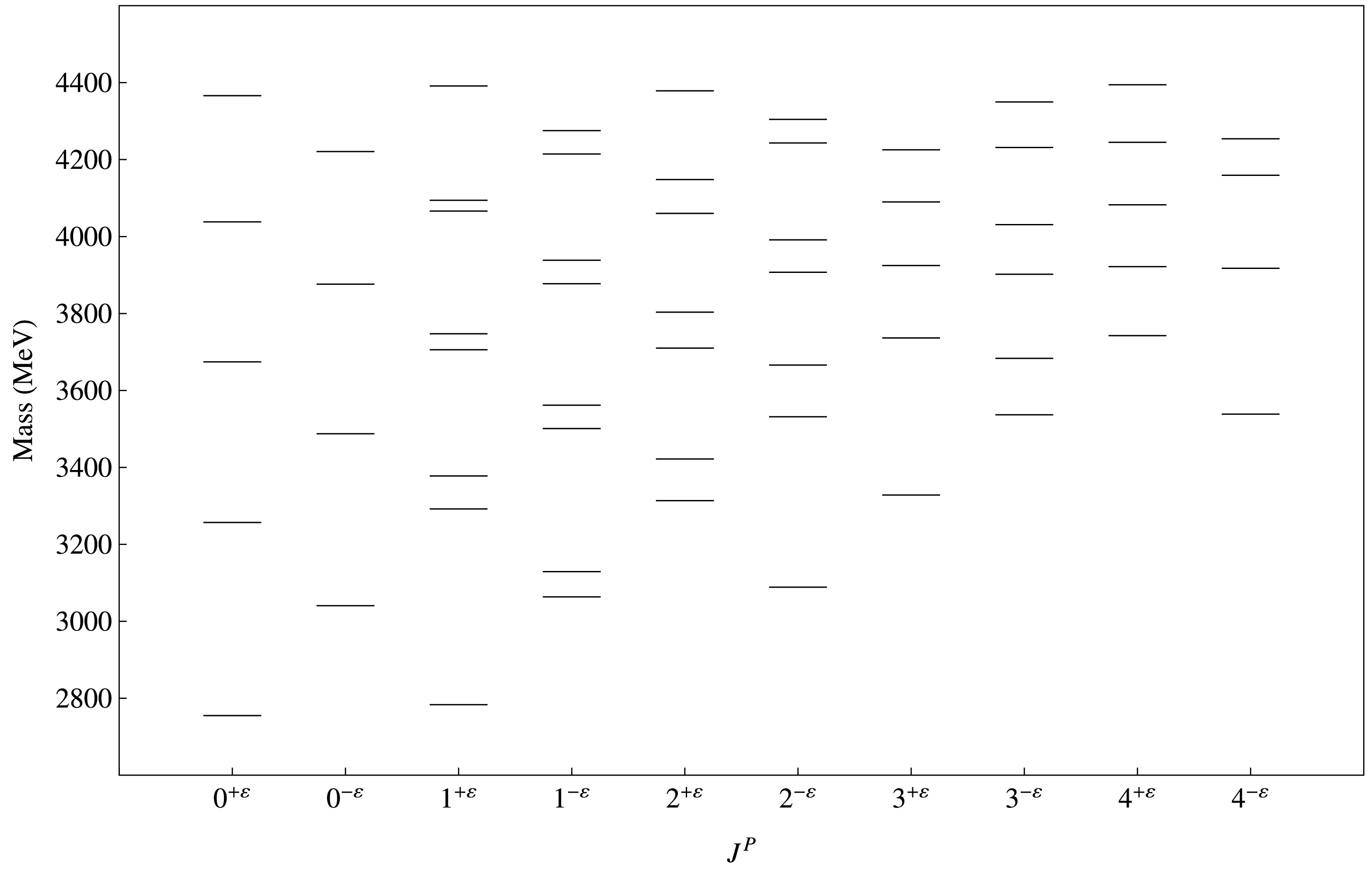
Figure 4.  Hybrid charmed mesons spectrum.

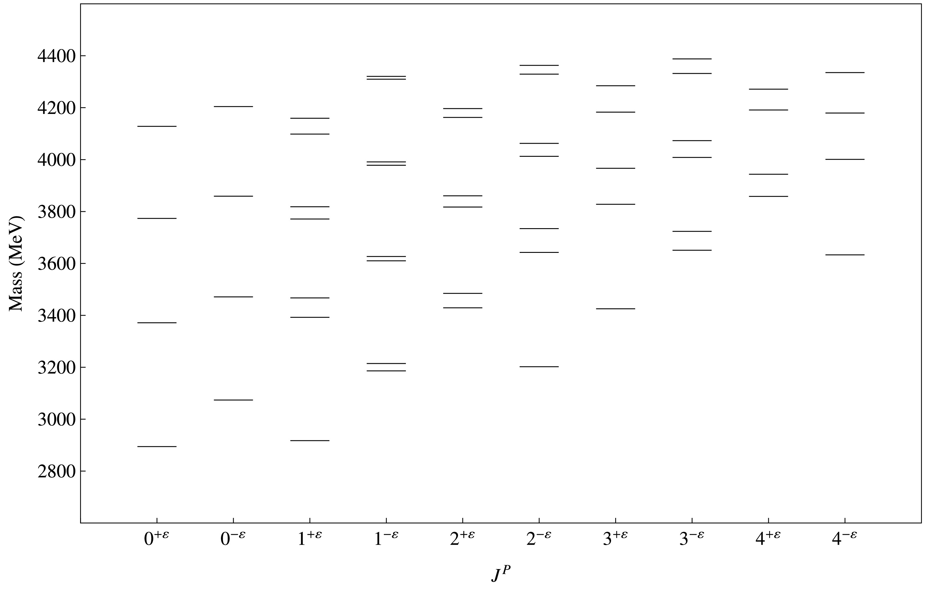
Figure 5.  Hybrid charmed strange mesons spectrum.

Meson	$ J^P $	Our Results	GI Model [20]	[22]	[39]	Exp. Data
Charmed strange mesons:
$ D_{s0}^*(2590)^+ $	0-	2659	2673	2582	2557	2591±9 [49]
$ D_{sJ}^*(3040)^\pm $	1+, 2+	3026.94, 3077.36				$ 3044_{-9}^{+31} $ [48]
Charmed mesons:
$ D_0(2550)^0 $	0-	2553.34	2581	2483		2549 ± 19 [50, 51]
$ D_1^*(2600)^0 $	1-	2618.66	2643	2613		2627 ± 10 [51, 52]
$ D_2(2740)^0 $	2-	2752.03	2816	2737		2747 ± 6 [50, 53]
$ D_1^*(2760)^0 $	1-	2770.32	2817	2785		2781 ± 22 [54]
$ D(3000)^0 $	3+, 3-, 4-	3184.76, 3233.29, 3275.27				3214 ± 60 [52, 53]

Table 3.  Comparison of our calculated spectrum (in MeV) for conventional D and $ D_s $ mesons with those of other studies and experimental data.

Radiative transitions play a vital role in the identification of meson states. The E1 radiative partial width between initial and final mesons in the non-relativistic quark model is given by [55]

where $ \alpha $ = $ \dfrac{1}{137}\; $ is the electromagnetic fine structure constant, $ \omega $ is photon energy, $ \lvert{n^{2S+1}L_J}\rangle $ is the initial meson state, $ \lvert{n'^{2S'+1}L'_{J'}}\rangle $ is the final meson state, $ E_f $ is the energy of final meson state, and $ M_i $ is the mass of the initial meson. $ C_{fi} $ is the angular momentum matrix element and is defined as

where $ \begin{Bmatrix}.&.&.\\.&.&. \end{Bmatrix}\; $ is a 6-j symbol. In Eq. (33), $ \langle {e_Q} \rangle $ is

Here, $ m_c $ and $ m_{q} $ are the constituent masses of the charm and light (q) quarks, respectively. For the D meson, q = u/d and for the $ D_s $ meson, q = s. $ e_{\overline{c}}$ = –2/3 is the electric charge of the anti-charm quark in units of $ |e| $. $ e_u $ = +2/3, $ e_d$ = –1/3, and $ e_s$ = –1/3 are electric charges of up, down, and strange quarks, respectively, in units of $ |e| $.

Matrix elements $ \langle {n'^{2S'+1}L'_{J'}} | {r} | {n^{2S+1}L_J}\rangle $ are calculated using the relativistic quark model wave functions obtained in Section IV. In E1 transitions, relativistic corrections are implicitly included due to the contribution of spin dependent interactions in the Hamiltonian.

The M1 radiative partial width of the S-wave meson bound state is [20]

where $ j_0 $ is the spherical Bessel function. Electromagnetic transitions are sensitive to the internal structure of mesons, particularly in the case of mixed states. A mixed state is a linear combination of two states; only the component(s) that satisfy the selection rules for E1 and M1 transitions contribute to the transition amplitude. To calculate the decay width of M1 transitions for conventional S-wave meson bound states, the M1 selection rules and Eq. (28) imply that only the $ 1^{-}\leftrightarrow 0^{-} $ transition is allowed. Furthermore, only the $ ^{3}S_{1} $ component of the 1^– state contributes to the decay width. To calculate the decay width of E1 transitions of conventional meson bound states ($ L<3 $), the selection rules of E1 transitions and Eqs. (22, 28) indicate that only four transitions contribute, i.e., $ 1^{+}\leftrightarrow 0^{-} $, $ 1^{-}\leftrightarrow 0^{+} $, $ 1^{-}\leftrightarrow 1^{+} $, and $ 2^{-}\leftrightarrow 1^{+} $. In the $ 1^{+}\leftrightarrow 0^{-} $ transition, only the $ {}^{1}P_1 $ component of the 1⁺ state fulfil the selection rule of the E1 transitions. In the $ 1^{-}\leftrightarrow 0^{+} $ transition, both the components of the 1^– state have contributions. For the $ 1^{-}\leftrightarrow 1^{+} $ transition, both components of the initial and final states contribute except the $ {}^{1}P_{1} $ component of the 1⁺ state. Finally, in the $ 2^{-}\leftrightarrow 1^{+} $ transition, both components of the initial and final states contribute.

In this work, we present a detailed spectrum of conventional and hybrid charmed and charmed strange mesons. States with the same $ J^P $ quantum numbers are treated as mixed states. We have incorporated both spin and S-D mixing through the off-diagonal matrix elements of the Hamiltonian. In Figs. 2 to 5, state mixing phenomena are explicitly visualized by the spectrum pattern. Ref. [20] includes spin mixing effects, although S-D mixing is ignored in the calculations therein. In Ref. [22], the spin dependent Hamiltonian part is added perturbatively after solving the eigenequation. In this study, we use the complete Hamiltonian, including the spin dependent part, in the eigenvalue equation. This approach enables us to study both spin effects and S-D mixing without resorting to perturbation theory.

Our calculated spectrum of conventional D and $ D_s $ mesons is reported in Table 4 with increasing mass. n is the number of eigenvalues associated with a specific value of $ J^P $. For unmixed states, the 0⁺ ($ {}^3P_0 $) states have a larger mass than the 0^– ($ {}^1S_0 $) states due to spin and orbital excitation. For S-D mixed states, higher orbital excited states (e.g., 2⁺, $ {}^3P_2 \leftrightarrow {}^3F_2 $) have larger masses than lower excited states (e.g., 1^–, $ {}^3S_1 \leftrightarrow {}^3D_1 $). The same is observed for the spin singlet and spin triplet mixed states. States with higher orbital excitations (e.g., 2^–, $ {}^1D_2 \leftrightarrow {}^3D_2 $) have larger masses than lower orbital excited states (e.g., 1⁺, $ {}^1P_1 \leftrightarrow {}^3P_1 $). We also compare our calculated spectrum of conventional D and $ D_s $ mesons with experimental results and the results of other studies in Tables 2 and 3. Our results show good agreement with both previous study findings and experimental data. We used meson states in Table 2 for fitting the parameter values. Table 3 shows the efficiency of our results. In Table 3, we identify $ D_{sJ}^*(3040)^\pm $ and $ D(3000)^0 $ as the 1⁺ and 3^– states, respectivley. We tentatively identify $ D_{sJ}^*(3040)^\pm $ and $ D(3000)^0 $ as the 2⁺ and 3⁺ states, respectively. $ D(3000)^0 $ could be considered the 4^– state. Because the nature of the $ D^*_{s0}(2317)^{\pm} $ and $ D_{s1}(2460)^{\pm} $ states is unclear, as discussed in Section I, we did not include these states in the fitting procedure. Moreover, we did not find any good matches for these states in either the conventional or hybrid mass spectrum. This result is consistent with the previously suggested exotic nature of $ D_{s0}^*(2317) $ and $ D_{s1}(2460) $ mesons.

$ J^P $	n	D Meson	$ D_s $ Meson
$0^-$	1	1890.66	2001.36
	2	2553.34	2659.00
	3	3070.94	3162.90
	4	3491.35	3581.01
$0^+$	1	2334.64	2221.26
	2	2895.60	2830.25
	3	3339.03	3292.43
	4	3723.79	3684.70
$1^-$	1	1980.63	2079.63
	2	2618.66	2706.22
	3	2770.32	2820.59
	4	3111.91	3170.35
	5	3210.21	3218.06
	6	3524.85	3561.34
	7	3599.51	3614.62
	8	3888.75	3912.91
$1^+$	1	2391.87	2514.83
	2	2458.56	2535.92
	3	2880.36	3012.05
	4	2955.80	3026.94
	5	3327.55	3435.81
	6	3400.51	3446.24
	7	3710.89	3807.50
	8	3784.40	3816.56
$2^-$	1	2752.03	2857.35
	2	2862.13	2911.54
	3	3188.32	3292.05
	4	3287.53	3327.83
	5	3571.28	3672.60
	6	3666.60	3699.38
	7	3916.99	4014.94
	8	4008.79	4037.37
$2^+$	1	2464.39	2569.18
	2	2959.26	3077.36
	3	3131.47	3203.58
	4	3379.56	3483.48
	5	3494.62	3539.61
	6	3750.46	3819.04
	7	3840.78	3881.70
	8	4086.20	4130.11
$3^-$	1	2789.59	2869.84
	2	3233.29	3320.75
	3	3448.43	3499.65
	4	3615.56	3702.96
	5	3765.23	3825.09
	6	3959.01	4053.21
	7	4075.86	4114.68
	8	4274.05	4363.43
$3^+$	1	3031.60	3138.04
	2	3184.76	3216.67
	3	3427.33	3529.81
	4	3560.11	3594.36
	5	3781.48	3881.76
	6	3904.52	3935.16
	7	4105.19	4203.53
	8	4222.14	4248.79
$4^-$	1	3275.27	3385.16
	2	3466.85	3480.50
	3	3634.65	3738.40
	4	3804.95	3826.51
	5	3971.98	4073.56
	6	4125.85	4149.44
	7	4278.55	4376.37
	8	4424.86	4445.97
$4^+$	1	3050.12	3128.49
	2	3460.14	3536.36
	3	3727.59	3740.77
	4	3819.37	3900.19
	5	4021.00	4050.96
	6	4144.89	4230.53
	7	4303.97	4357.16
	8	4445.31	4534.66

Table 4.  Calculated conventional D and $ D_s $ meson masses (in MeV) for $ J^P = 0^- $, 0⁺, 1^-, 1⁺, 2^-, 2⁺, 3^-, 3⁺, 4^-, and 4⁺.

In Table 5, we report the computed masses of hybrid D and $ D_s $ mesons. For hybrid candidates, the parity condition differs from that of conventional mesons owing to the contribution of the excited gluonic field, as discussed in Section I. It is observed that hybrid states have greater masses compared to conventional mesons. This occurs due to gluonic excitations in $ \Pi_u $ states. In Tables 6 and 7, we report our calculated E1 transitions for conventional to conventional and hybrid to hybrid mesons, respectively. We also present M1 transitions for conventional to conventional and hybrid to hybrid mesons in Tables 8 and 9, respectively. We observed that the decay width of $ D^0(c\bar{u}) $ states is larger than that of $ D^\pm(c\bar{d}) $ states, except for few states in M1 transitions. In Table 10, we compare our calculated radiative decay width of conventional mesons with those of other studies and experimental results. Our results are consistent with those of other studies except for those corresponding to a few $ D^0 $ meson states. We expect our predicted results to be useful for the detection of new charmed and charmed strange mesons.

$ J^P $	n	Hybrid D Meson	Hybrid $ D_s $ Meson
$0^{+\varepsilon}$	1	2755.01	2894.34
	2	3256.86	3371.39
	3	3674.27	3773.52
	4	4038.16	4128.21
$0^{-\varepsilon}$	1	3040.45	3073.69
	2	3487.44	3471.19
	3	3876.36	3858.93
	4	4220.98	4204.41
$1^{+\varepsilon}$	1	2783.31	2917.32
	2	3291.98	3392.35
	3	3377.88	3467.12
	4	3705.86	3771.09
	5	3747.28	3818.40
	6	4066.32	4098.38
	7	4094.33	4159.38
	8	4391.27	4406.70
$1^{-\varepsilon}$	1	3063.57	3186.10
	2	3129.03	3214.35
	3	3501.03	3610.14
	4	3561.83	3626.80
	5	3877.47	3978.27
	6	3938.51	3991.02
	7	4214.71	4309.78
	8	4275.42	4320.49
$2^{+\varepsilon}$	1	3313.71	3429.11
	2	3422.03	3484.54
	3	3710.06	3817.38
	4	3803.52	3860.47
	5	4060.25	4162.55
	6	4148.00	4196.43
	7	4378.76	4476.95
	8	4462.95	4504.55
$2^{-\varepsilon}$	1	3088.68	3202.11
	2	3531.70	3642.38
	3	3666.11	3734.10
	4	3907.27	4012.51
	5	3991.32	4062.51
	6	4243.29	4329.07
	7	4304.42	4363.03
	8	4550.91	4612.00
$3^{+\varepsilon}$	1	3328.26	3425.32
	2	3736.37	3827.75
	3	3924.76	3966.53
	4	4089.99	4182.79
	5	4225.45	4284.57
	6	4409.37	4503.65
	7	4512.24	4572.02
	8	4703.77	4797.78
$3^{-\varepsilon}$	1	3536.73	3650.73
	2	3683.47	3723.53
	3	3902.08	4008.45
	4	4030.85	4073.06
	5	4231.61	4331.70
	6	4349.85	4387.91
	7	4534.57	4619.30
	8	4645.99	4671.07
$4^{+\varepsilon}$	1	3742.56	3858.08
	2	3921.79	3943.51
	3	4082.66	4191.13
	4	4244.97	4271.20
	5	4394.41	4497.79
	6	4544.24	4572.21
	7	4683.88	4783.46
	8	4824.56	4852.37
$4^{-\varepsilon}$	1	3538.36	3633.01
	2	3917.60	4000.87
	3	4159.43	4179.46
	4	4254.05	4335.09
	5	4446.62	4483.56
	6	4560.83	4641.67
	7	4715.93	4763.97
	8	4845.22	4927.05

Table 5.  Calculated hybrid D and $ D_s $ meson masses (in MeV) for $ J^P $ = $ 0^{-\varepsilon} $, $ 0^{+\varepsilon } $, $ 1^{-\varepsilon} $, $ 1^{+\varepsilon} $, $ 2^{-\varepsilon} $, $ 2^{+\varepsilon} $, $ 3^{-\varepsilon} $, $ 3^{+\varepsilon} $, $ 4^{-\varepsilon} $, and $ 4^{+\varepsilon} $.

Transition	Initial state $ nJ^{P} $	Final state $ nJ^{P} $	$ \Gamma_{e1} $(D meson) ($ c\bar{u} $, $ c\bar{d} $)	$ \Gamma_{e1} $($ D_s $ meson)
$0^- \rightarrow 1^+\gamma$	$20^-$	$11^+$	91.149, 3.457	0.4176
		$21^+$	75.435, 1.9573	0.2435
	$30^-$	$11^+$	210.5, 5.8748	0.3448
		$21^+$	226.65, 5.8811	0.2216
		$31^+$	432.72, 11.228	1.049
		$41^+$	109.09, 2.8305	0.697
$0^+ \rightarrow 1^-\gamma$	$10^+$	$11^-$	728.01, 19.4031	0.0859
	$20^+$	$11^-$	184.37, 4.8241	2.0001
		$21^-$	545.88, 14.164	0.2027
		$31^-$	35.948, 0.9328	0.0002
	$30^+$	$11^-$	47.770, 1.2456	0.3441
		$21^-$	290.88, 7.5475	1.6971
		$31^-$	407.65, 10.577	1.6964
		$41^-$	748.15, 19.413	0.5871
		$51^-$	158.37, 4.1092	0.162
$1^- \rightarrow 0^+\gamma$	$21^-$	$10^+$	43.527, 1.1612	1.9786
	$31^-$	$10^+$	628.92, 16.779	3.8272
	$41^-$	$10^+$	776.18, 20.707	0.1186
		$20^+$	604.83, 16.136	2.8181
	$51^-$	$10^+$	49.96, 1.3328	0.2344
		$20^+$	604.83, 16.136	2.8181
$1^- \rightarrow 1^+\gamma$	$21^-$	$11^+$	82.384, 2.7702	0.4364
		$21^+$	73.119, 1.8973	0.291
	$31^-$	$11^+$	497.36, 14.921	1.6613
		$21^+$	463.44, 12.025	1.263
	$41^-$	$11^+$	1028.9, 28.573	0.9155
		$21^+$	1016.9, 26.386	0.5979
		$31^+$	383.55, 9.9521	0.6226
		$41^+$	133.93, 3.4751	0.4148
	$51^-$	$11^+$	234.27, 6.4414	0.5734
		$21^+$	244.65, 6.3481	0.3518
		$31^+$	1126.6, 29.234	1.1176
		$41^+$	585.33, 15.188	0.7807
$1^+ \rightarrow 0^-\gamma$	$11^+$	$10^-$	847.18, 20.415	3.4365
	$21^+$	$10^-$	886.97, 23.498	3.7954
	$31^+$	$10^-$	0.123, 0.0032	0.1012
		$20^-$	443.01, 11.495	2.1211
	$41^+$	$10^-$	0.7203, 0.0189	0.0009
		$20^-$	764.76, 19.844	2.7341
$1^+ \rightarrow 1^-\gamma$	$11^+$	$11^-$	638.97, 14.809	2.2145
	$21^+$	$11^-$	851.13, 22.510	2.526
	$31^+$	$11^-$	80.893, 2.1169	0.4596
		$21^-$	313.77, 8.1415	1.8567
		$31^-$	4.6457, 0.1205	0.3447
	$41^+$	$11^-$	106.76, 2.7914	0.5276
		$21^-$	622.18, 16.144	2.2821
		$31^-$	20.975, 0.5442	0.4659
$1^+ \rightarrow 2^-\gamma$	$31^+$	$12^-$	65.085, 1.6888	0.5529
		$22^-$	0.2119, 0.0055	0.1558
	$41^+$	$12^-$	238.29, 6.1831	0.8464
		$22^-$	26.278, 0.6818	0.2738
	$51^+$	$12^-$	1.3736, 0.0356	0.1362
		$22^-$	5.0118, 0.13	0.1717
		$32^-$	181.45, 4.7082	0.998
		$42^-$	5.0814, 0.1318	0.4126
	$61^+$	$12^-$	2.6022, 0.0675	0.2015
		$22^-$	0.6375, 0.0165	0.2359
		$32^-$	554.7, 14.393	1.3456
		$42^-$	99.485, 2.5814	0.5961
$2^- \rightarrow 1^+\gamma$	$12^-$	$11^+$	1324.5, 40.073	5.3991
		$21^+$	1235.9, 32.0705	4.27
	$22^-$	$11^+$	2821.6, 81.961	8.0433
		$21^+$	2692.4, 69.861	6.5345
	$32^-$	$11^+$	135.6, 3.736	0.0116
		$21^+$	154.87, 4.0186	0.0318
		$31^+$	1541.9, 40.008	4.8947
		$41^+$	746.69, 19.375	3.7323
	$42^-$	$11^+$	167.93, 4.589	0.0259
		$21^+$	194.43, 5.045	0.0352
		$31^+$	3316.8, 86.062	6.8996
		$41^+$	2019.9, 52.411	5.3872

Table 6.  Partial widths of the E1 decays (in keV) of conventional D and $ D_s $ mesons.

Transition	Initial state $ nJ^{P} $	Final state $ nJ^{P} $	$ \Gamma_{e1} $(hybrid D meson) ($ c\bar{u} $, $ c\bar{d} $)	$ \Gamma_{e1} $(hybrid $ D_s $ meson)
$0^{+\varepsilon} \rightarrow 1^{-\varepsilon}\gamma$	$20^{+\varepsilon}$	$11^{-\varepsilon}$	261.12, 6.7754	1.059
		$21^{-\varepsilon}$	81.811, 2.1228	0.6407
	$30^{+\varepsilon}$	$11^{-\varepsilon}$	57.046, 1.4802	0.2516
		$21^{-\varepsilon}$	60.926, 1.5809	0.2588
		$31^{-\varepsilon}$	385.99, 10.016	1.5485
		$41^{-\varepsilon}$	117.44, 3.0472	1.0873
$0^{-\varepsilon} \rightarrow 1^{+\varepsilon}\gamma$	$10^{-\varepsilon}$	$11^{+\varepsilon}$	618.71, 16.054	0.4149
	$20^{-\varepsilon}$	$11^{+\varepsilon}$	387.02, 10.0423	1.9049
		$21^{+\varepsilon}$	264.43, 6.8614	0.0996
		$31^{+\varepsilon}$	63.071, 1.6365	0.00002
	$30^{-\varepsilon}$	$11^{+\varepsilon}$	6.5882, 0.1709	0.2337
		$21^{+\varepsilon}$	251.11, 6.5156	1.8328
		$31^{+\varepsilon}$	153.29, 3.9775	2.48
		$41^{+\varepsilon}$	301.26, 7.817	0.3068
		$51^{+\varepsilon}$	158.79, 4.1204	0.0377
$1^{+\varepsilon} \rightarrow 0^{-\varepsilon}\gamma$	$21^{+\varepsilon}$	$10^{-\varepsilon}$	199.35, 5.3184	1.3168
	$31^{+\varepsilon}$	$10^{-\varepsilon}$	511.52, 13.646	2.395
	$41^{+\varepsilon}$	$10^{-\varepsilon}$	3.2826, 0.0876	0.0766
		$20^{-\varepsilon}$	231.81, 6.1844	2.0572
	$51^{+\varepsilon}$	$10^{-\varepsilon}$	16.243, 0.4333	0.2632
		$20^{-\varepsilon}$	417.04, 11.126	2.48
$1^{+\varepsilon} \rightarrow 1^{-\varepsilon}\gamma$	$21^{+\varepsilon}$	$11^{-\varepsilon}$	222.27, 5.7673	0.7543
		$21^{-\varepsilon}$	85.868, 2.2281	0.4825
	$31^{+\varepsilon}$	$11^{-\varepsilon}$	436.29, 11.3207	1.7273
		$21^{-\varepsilon}$	229.88, 5.9648	1.2476
	$41^{+\varepsilon}$	$11^{-\varepsilon}$	71.744, 1.8616	0.4743
		$21^{-\varepsilon}$	61.15, 1.5867	0.3914
		$31^{-\varepsilon}$	303.65, 7.8791	0.8211
		$41^{-\varepsilon}$	115.48, 2.9963	0.5718
	$51^{+\varepsilon}$	$11^{-\varepsilon}$	132.82, 3.4463	0.1873
		$21^{-\varepsilon}$	113.01, 2.9322	0.156
		$31^{-\varepsilon}$	374.27, 9.7114	1.452
		$41^{-\varepsilon}$	174.23, 4.5208	1.0843
$1^{-\varepsilon} \rightarrow 0^{+\varepsilon}\gamma$	$11^{-\varepsilon}$	$10^{+\varepsilon}$	420.74, 10.917	1.4283
	$21^{-\varepsilon}$	$10^{+\varepsilon}$	714.93, 18.551	1.8474
	$31^{-\varepsilon}$	$10^{+\varepsilon}$	21.638, 0.5615	0.000008
		$20^{+\varepsilon}$	350.18, 9.0864	1.3169
	$41^{-\varepsilon}$	$10^{+\varepsilon}$	23.361, 0.6062	0.0033
		$20^{+\varepsilon}$	652.03, 16.918	1.6334
$1^{-\varepsilon}\rightarrow 1^{+\varepsilon}\gamma$	$11^{-\varepsilon}$	$11^{+\varepsilon}$	462.52, 12.001	1.4309
	$21^{-\varepsilon}$	$11^{+\varepsilon}$	827.38, 21.468	1.8929
	$31^{-\varepsilon}$	$11^{+\varepsilon}$	163.51, 4.2426	0.5119
		$21^{+\varepsilon}$	265.17, 6.8805	1.2207
		$31^{+\varepsilon}$	49.942, 1.2959	0.473
	$41^{-\varepsilon}$	$11^{+\varepsilon}$	196.41, 5.0965	0.577
		$21^{+\varepsilon}$	543.57, 14.104	1.5197
		$31^{+\varepsilon}$	158.73, 4.1187	0.6515
$1^{-\varepsilon} \rightarrow 2^{+\varepsilon}\gamma$	$31^{-\varepsilon}$	$12^{+\varepsilon}$	251.90, 6.5361	1.0387
		$22^{+\varepsilon}$	22.292, 0.5784	0.3843
	$41^{-\varepsilon}$	$12^{+\varepsilon}$	549.57, 14.26	1.3888
		$22^{+\varepsilon}$	116.31, 3.0179	0.5716
	$51^{-\varepsilon}$	$12^{+\varepsilon}$	12.435, 0.3227	0.0632
		$22^{+\varepsilon}$	30.026, 0.7791	0.1367
		$32^{+\varepsilon}$	377.98, 9.8075	1.5399
		$42^{+\varepsilon}$	38.496, 0.9989	0.6371
	$61^{-\varepsilon}$	$12^{+\varepsilon}$	1.709, 0.0443	0.0708
		$22^{+\varepsilon}$	18.596, 0.4825	0.1541
		$32^{+\varepsilon}$	860.24, 22.321	2.0341
		$42^{+\varepsilon}$	211.48, 5.4873	0.9093
$2^{+\varepsilon} \rightarrow 1^{-\varepsilon}\gamma$	$12^{+\varepsilon}$	$11^{-\varepsilon}$	872.62, 22.642	3.3811
		$21^{-\varepsilon}$	373.06, 9.6801	2.3478
	$22^{+\varepsilon}$	$11^{-\varepsilon}$	2390.7, 62.033	6.0388
		$21^{-\varepsilon}$	1386.2, 35.968	4.5079
	$32^{+\varepsilon}$	$11^{-\varepsilon}$	74.05, 1.9214	0.0924
		$21^{-\varepsilon}$	74.711, 1.9386	0.0787
		$31^{-\varepsilon}$	736, 19.097	3.0566
		$41^{-\varepsilon}$	284.58, 7.3841	2.3242
	$42^{+\varepsilon}$	$11^{-\varepsilon}$	57.592, 1.4944	0.0451
		$21^{-\varepsilon}$	66.767, 1.7324	0.0386
		$31^{-\varepsilon}$	2063.6, 53.545	5.1521
		$41^{-\varepsilon}$	1143.8, 29.679	4.0959

Table 7.  Partial widths of the E1 decays (in keV) of hybrid D and $ D_s $ mesons.

Transition	Initial state $ nJ^{P} $	Final state $ nJ^{P} $	$ \Gamma_{m1} $(D meson) ($ c\bar{u} $, $ c\bar{d} $)	$ \Gamma_{m1} $($ D_s $ meson)
$ 0^- \rightarrow 1^-\gamma $	$ 20^- $	$ 11^- $	11.097, 7.4747	2.184
	$ 30^- $	$ 11^- $	0.1487, 6.2222	2.3694
		$ 21^- $	22.198, 10.062	2.9894
		$ 31^- $	98.771, 1.2647	0.209
	$ 40^- $	$ 11^- $	0.1319, 1.566	0.5123
		$ 21^- $	25.08, 18.489	5.9304
		$ 31^- $	248.86, 10.857	0.1343
		$ 41^- $	16.733, 7.8301	3.7441
		$ 51^- $	68.052, 0.0079	2.0575
$ 1^- \rightarrow 0^-\gamma $	$ 11^- $	$ 10^- $	23.648, 0.6064	0.0665
	$ 21^- $	$ 10^- $	127.55, 17.5012	4.0203
		$ 20^- $	2.5479, 0.0644	0.0042
	$ 31^- $	$ 10^- $	2085, 19.985	7.9164
		$ 20^- $	4.8418, 0.19	0.0919
	$ 41^- $	$ 10^- $	112.9, 17.719	1.622
		$ 20^- $	82.281, 10.879	1.9332
		$ 30^- $	0.6405, 0.0163	0.00001
	$ 51^- $	$ 10^- $	1350, 0.9538	5.1259
		$ 20^- $	42.254, 1.3827	2.8697
		$ 30^- $	7.1297, 0.123	0.004

Table 8.  Partial widths of the M1 decays (in keV) of conventional D and $ D_s $ mesons.

Transition	Initial state $ nJ^{P} $	Final state $ nJ^{P} $	$ \Gamma_{m1} $(hybrid D meson) ($ c\bar{u} $, $ c\bar{d} $)	$ \Gamma_{m1} $(hybrid $ D_s $ meson)
$ 0^{+\varepsilon} \rightarrow 1^{+\varepsilon}\gamma $	$ 20^{+\varepsilon} $	$ 11^{+\varepsilon} $	22.206, 9.4979	2.1082
	$ 30^{+\varepsilon} $	$ 11^{+\varepsilon} $	8.4751, 10.6	2.2568
		$ 21^{+\varepsilon} $	14.759, 6.9874	2.1905
		$ 31^{+\varepsilon} $	2.6918, 1.303	0.5497
	$ 40^{+\varepsilon} $	$ 11^{+\varepsilon} $	9.428, 5.1214	0.7265
		$ 21^{+\varepsilon} $	21.874, 16.759	4.8863
		$ 31^{+\varepsilon} $	13.313, 3.7718	0.6848
		$ 41^{+\varepsilon} $	12.489, 5.5476	2.5828
		$ 51^{+\varepsilon} $	10.924, 2.235	1.2671
$ 1^{+\varepsilon} \rightarrow 0^{+\varepsilon}\gamma $	$ 11^{+\varepsilon} $	$ 10^{+\varepsilon} $	0.2161, 0.0056	0.0003
	$ 21^{+\varepsilon} $	$ 10^{+\varepsilon} $	53.308, 7.458	1.1989
		$ 20^{+\varepsilon} $	0.4085, 0.0105	0.0002
	$ 31^{+\varepsilon} $	$ 10^{+\varepsilon} $	425.28, 17.191	2.2738
		$ 20^{+\varepsilon} $	12.745, 0.2962	0.0171
	$ 41^{+\varepsilon} $	$ 10^{+\varepsilon} $	60.381, 11.716	0.9809
		$ 20^{+\varepsilon} $	46.49, 6.0773	0.9054
	$ 51^{+\varepsilon} $	$ 10^{+\varepsilon} $	760.03, 29.874	2.861
		$ 20^{+\varepsilon} $	234.39, 9.8806	1.5053
		$ 30^{+\varepsilon} $	2.5875, 0.0632	0.0022

Table 9.  Partial widths of the M1 decays (in keV) of hybrid D and $ D_s $ mesons.

Mode	Our Results	GI Model [20]	[56]	[57]	[39]	PDG [18]
Charmed strange mesons
$ D_s^{*\pm} \rightarrow D_s^{\pm}\gamma $	0.0665	1.03	2.39	1.12		< 1776.5
$ D_{s1}(2536)^\pm \rightarrow D_s^{\pm}\gamma $	3.7954	9.23	61.2	37.7	3.53
$ D_{s1}(2536)^\pm \rightarrow D_s^{*\pm}\gamma $	2.526	9.61	9.21	5.74	4.74
Charmed mesons ($ c\bar{u} $)
$ D^*(2007)^{0} \rightarrow D^{0}\gamma $	23.648	106				< 741
$ D_0^{*}(2300)^{0} \rightarrow D^{*}(2007)^{0}\gamma $	728.01	288
$ D_1(2430)^{0} \rightarrow D^{0}\gamma $	847.18	640
$ D_1(2420) \rightarrow D^{0}\gamma $	886.97	156
$ D_1(2430)^{0} \rightarrow D^{*}(2007)^{0}\gamma $	638.97	82.8
$ D_1(2420) \rightarrow D^{*}(2007)^{0}\gamma $	851.13	386
Charmed mesons ($ c\bar{d} $)
$ D^*(2010)^{\pm}\rightarrow D^{\pm}\gamma $	0.6064	10.8				≈ 1.334
$ D_0^{*} \rightarrow D^{*}(2010)^{\pm}\gamma $	19.4031	30
$ D_1 \rightarrow D^{\pm}\gamma $	20.415	66
$ D_1^{'}\rightarrow D^{\pm}\gamma $	23.498	16.1
$ D_1 \rightarrow D^{*}(2010)^{\pm}\gamma $	14.809	8.6
$ D_1^{'} \rightarrow D^{*}(2010)^{\pm}\gamma $	22.51	39.9

Table 10.  Comparison of our calculated radiative decay partial widths (in keV) with those of other studies. $ D_1 $ and $ D_1^{'} $ are the mixed states ($ J^P = 1^+ $) of charmed mesons.