Probing D_s^*-meson longitudinal twist-2 LCDA

B-meson semileptonic decay is a very important tool for studying the weak interaction. It has great phenomenological implications within the Standard Model (SM) of particle physics.$ B_s\to D_s^*\ell \bar\nu_{\ell} $ decay provides an opportunity for extracting CKM matrix elements and testing the SM [1−4]. Recently, the study of $ B_s\to D_s^*\ell \bar\nu_{\ell} $has attracted significant interest, driven by advancements in experimental capabilities and theoretical developments. Many experiments have provided increasingly precise data of these decays, which allow the extraction of the CKM matrix element to an increasingly better accuracy. In addition, many theoretical groups have shown great interest in exploring the decay channel.

In 2020, the LHCb Collaboration [5, 6] published an article on the experimental measurement of $ B_s\to D_s^*\ell \bar\nu_{\ell} $ decay. They used the experimental data samples collected by the LHCb detector at center-of-mass energies of 7 and 8 TeV and conducted systematic studies on the two decay channels $ B^0_s\to D^-_s\mu^+\nu_\mu $ and $ B^0_s\to D^{*-}_s\mu^+\nu_\mu $ using Caprini-Lellouch-Neubert (CLN) and Boyd-Grinstein-Lebed (BGL) parameterizations. The final measured values of $ |V_{cb}| $obtained under the two parameterizations were $ (41.4 \pm 0.6 \pm 0.9 \pm 1.2)\times10^{-3} $ and $ (42.3 \pm 0.8\pm 0.9 \pm 1.2)\times 10^{-3} $, respectively. In Ref. [7], the lattice QCD and HPQCD Collaboration worked together to determine the model independent value of $ V_{cb} = 39.03(56)_{\rm{exp.}} (67)_{\rm{latt.}}\times 10^{-3} $ using the $ B\to D^{*}\ell \bar{\nu}_{\ell} $ data from Belle and the $ B_s\to D_s^*\mu \bar{\nu}_\mu $ data from LHCb, as well as their own transition form factors (TFFs). The TFFs and decay width behaviors for the $ B_s\to D_s^*\ell \bar{\nu}_{\ell} $ process were also given in that article.

Theoretically, there are many methods for making reasonable predictions of $ B_s\to D_s^*\ell \bar\nu_{\ell} $ decay, such as lattice QCD (LQCD) [8−12], soft-collinear effective theory (SCET) [13], covariant confined quark model (CCQM) [14], QCD sum rules (QCDSR) [15], relativistic quark model (RQM) [16], perturbative QCD (pQCD) [17, 18], light-front quark model (LFQM) [19], and Bethe-Salpeter method [20]; here, we provides a brief introduction to the above methods. In Ref. [9], the SM semileptonic vector and axial-vector form factors for $ B_s \to D_s^* $ decay are calculated via the LQCD. The relevant calculation methods, the dependence on the heavy quark mass, decay rates and ratios are analysed. Meanwhile, the consistency with LHCb results and the tests on the impact of new physics couplings are also discussed. They give a reasonable reference to study the semileptonic decay of $ B_s \to D_s^* \ell \bar\nu_{\ell} $. In Ref. [13], the authors utilized the power-counting scheme for the first time to calculate the next-to-leading order (NLO) QCD corrections to the form factors of $ \bar{B}_{(s)}\to D_{(s)}^{(*)}\ell \bar\nu_{\ell} $ transitions in the large recoil region. Within the framework of SCET, they also improved the light-cone sum rules for these form factors and conducted a combined fit for the considered form factors. This significantly refined the previous measurements of the lepton flavor universality ratios. In Ref. [14], the author relied on the SM framework based on the CCQM to calculate TFFs within the entire dynamical category of squared momentum transfer for semileptonic decays. The obtained results, such as decay width ratios, show a degree of consistency with LHCb experiments and LQCD simulations, and the behaviors of differential decay distributions were compared. Other physical observations were also calculated. Through calculation, $ R(D_s) = 0.271\pm0.069 $, $ R(D^*_s) = 0.240\pm0.038 $ were obtained, and the ratio of decay widths of the $ D_s $ and $ D_s^* $ channels in the muon meson mode $ \Gamma(B_s\to D_s\mu^+\nu_\mu)/ \Gamma(B_s\to D_s^*\mu^+\nu_\mu) = 0.451\pm0.093 $ was determined. In Ref. [15], the phenomenology of the b-flavored strange meson $ B^0_s $ was studied through the QCDSR. Specifically, this included the evaluation of the particle's mass and leptonic constant, as well as the study of the form factors of certain decays (such as $ \bar B^0_s \to D^+_s\ell^-\bar{\nu} $, $ \bar B^0_s\to D^{*+}_s\ell^-\bar{\nu} $, $ \bar B^0_s \to K^{*+}\ell^-\bar{\nu} $); at the same time, the two-body non-leptonic $ \bar B^0_s $ decays were calculated under the factorization approximation. Finally, the evaluation result of the $ S U(3)_F $ breaking effect in the $ \bar B^0_s $ channel was compared with other estimates.

Also, as a well-established theory that can be effectively applied to the exclusive decay process, the QCD light-cone sum rule (LCSR) [21, 22] incorporates both the hard and soft contributions in the computation of hadron transitions. In the LCSR method, the two-point correlation function of vacuum to meson is constructed for calculating heavy-to-light TFFs, where the matrix elements of nonlocal operators are considered in the light-cone region $ x^2 \to 0 $. The difference between this method and traditional SVZ sum rule [23] is that all non-perturbative dynamics are parameterized according to the light-cone distribution amplitudes (LCDAs) with progressively higher twists instead of quark and gluon condensates [24]. Currently, the LCSR has been widely applied to the study of B to light-flavor meson decays [25−30]. In this work, we adopt LCSR to calculate the $ B_s\to D^*_s $ TFFs. Specifically, due to the presence of both longitudinal $ (\|) $ and transverse $ (\perp) $ polarization states in vector mesons, employing traditional currents to construct correlation functions poses a challenge involving fifteen LCDAs. Therefore, to simplify the calculation process, we adopt chiral currents instead of traditional currents, allowing the contributions of twist-2 LCDA to dominate and eliminating contributions from other LCDAs. The specific procedure will be elaborated in the next section. Therefore, an accurate prediction of the twist-2 $ \phi_{2;D_s^*}^\|(x,\mu) $ is of great importance. In recent relevant studies, breakthrough progress has been achieved in theoretical calculations of heavy meson distribution amplitudes. For instance, in Refs. [31−33], heavy meson distribution amplitudes were determined based on the Large Momentum Effective Theory and by utilizing the LQCD method. Furthermore, the amplitudes of $ D_s^* $-mesons were studied in these articles [34, 35], indicating that the research on $ D_s^* $-meson amplitudes has attracted considerable attention. Currently, the LCDA of many mesons depends on the Gegenbauer moment, which can be calculated using QCD sum rules. As a mature theoretical method, the background field theory (BFT) decomposes the quark field into a classical background field that describes non-perturbative effects and a quantum field that describes perturbative effects. This can provide a clean physical picture for separating the perturbative and non-perturbative properties of the QCD theory and provide a systematic way to derive the QCDSR for hadron phenomenology. Meanwhile, due to the ability to adopt different gauges for quantum fluctuations and the background field in BFT, the calculations can be greatly simplified. In our previous work, the longitudinal twist-2 LCDA of ρ-meson was successfully studied in BFT and constructed by the light cone harmonic oscillator (LCHO) model [36]. Motivated by this, in this work, we employ the BFT method to study the twist-2 LCDA of the $ D_s^* $-meson and attempt to integrate the phenomenological LCHO model to provide another perspective to understand the momentum distribution of quarks and gluons inside $ D_s^* $-mesons.

The remainder of this article is organized as follows. In Sec. II, we derive the summation rules for the ξ-moments of the $ D_s^* $-meson longitudinal leading-twist $ \phi_{2;D_s^*}^\|(x,\mu) $ LCDAs and $ B_s\to D_s^* $ TFFs $ A_1(q^2) $, $ A_2(q^2) $, and $ V(q^2) $, as well as establish the LCHO for the $ D_s^* $-meson leading-twist LCDAs. In Sec. III, we provide relevant numerical results and a detailed discussion. Section IV summarizes the article.

The differential decay width of semileptonic decays $ B_s\to D_s^*\ell\bar\nu_\ell $ can be written in terms of the helicity components basis [37−39]:

where the Fermi coupling constant $ G_F = 1.1663787(6)\times 10^{-5}\; {\rm{GeV}}^{-2} $, $ |V_{cb}| $ is the CKM matrix element, $ \lambda\equiv \lambda(m_{B_s}^2,m_{m_{D_s^*}}^2,q^2) = m_{B_s}^4+m_{D_s^*}^4+q^4-2(m_{B_s}^{2}m_{D_s^*}^{2}+m_{B_s}^{2}q^{2}+m_{D_s^*}^{2}q^{2}) $ is the phase-space factor, $ m_\ell $ is the lepton mass $ (\ell = e,\mu,\tau) $, and $ {\cal{H}}_{\rm{total}} $ represents the overall helicity structure:

The symbols $ {\cal{H}}_{I}(I = U,L,S) $are the bilinear combinations of the helicity components of the hadronic tensor. In this study, the leptonic mass $ m_\ell $ is very small in case of $ \ell = (e,\mu) $ when compared with the squared transition momentum $ q^2 $, which can be safely neglected. Thus, only two helicity structures remain, i.e., $ {\cal{H}}_U $ and $ {\cal{H}}_L $, which have the following formulas:

The helicity amplitudes $ H_i $ with index $ i = (\pm,0,t) $ are denoted as functions of invariant mass $ q^2 $, which are formed from the $ B_s\to D_s^* $ TFFs with different combinations:

As we know, the three $ B_s\to D_s^* $ TFFs $ A_1(q^2) $, $ A_2(q^2) $, and $ V(q^2) $ are the important hadronic inputs for studying the relevant implications of semileptonic decays $ B_s\to D_s^*\ell\bar\nu_\ell $. Therefore, to derive their analytic expressions within the LCSR approach, we construct the following chiral current correlation function (correlator):

where $ J_\mu(x) = \bar c(x)\gamma_\mu (1-\gamma_5)b(x) $ and $ J_{B_s}^\dagger(0) = $ $\bar b(0){\rm i} (1- \gamma_5)s(0) $ represent the left-handed current. As the $ D_s^* $-meson DAs are relatively complex structures, there are both chiral-even and chiral-odd DAs for the$ D_s^* $-meson, which has longitudinal and transverse polarization states. The adopted left-handed current can effectively highlight the contributions from the chiral-even DAs such as $ \phi_{2;D_s^*}^\|(x,\mu) $, $ \phi_{3;D_s^*}^{\bot}(x,\mu) $, $ \psi_{3;D_s^*}^{\bot}(x,\mu) $, $ \Phi_{3;D_s^*}^\|(x,\mu) $, $ \tilde{\Phi}_{3;D_s^*}^\|(x,\mu) $, $ \phi_{4;D_s^*}^\|(x,\mu) $, and $ \psi_{4;D_s^*}^\|(x,\mu) $, while the chiral-odd DAs provide zero contributions. For the remaining chiral-even DAs, only $ \phi_{2;D_s^*}^\|, \phi_{3;D_s^*}^\bot(x,\mu) $, and $ \psi_{3;D_s^*}^\bot(x,\mu) $ account for dominant contributions to the LCSR, while other chiral-even DAs offer negligible contributions. Moreover, the twist-3 DAs $ \phi_{3;D_s^*}^\bot(x,\mu) $ and $ \psi_{3;D_s^*}^\bot(x,\mu) $ can be related to $ \phi_{2;D_s^*}^\|(x,\mu) $ under the Wandzura-Wilczek (WW) approximation [40, 41]:

Therefore, the longitudinal leading-twist $ \phi_{2;D_s^*}^\|(x,\mu) $ may provide a dominant contribution, either directly or indirectly.

The correlation function (5) is defined at both the time-like and space-like $ q^2 $-regions. According to the basic steps of LCSR, the correlation function can first be treated in the timelike $ q^2 $-region by inserting a complete set of intermediate hadronic states with the same quantum numbers as the current operator $ \bar{c} i(1+\gamma_5)s $. By separating the pole term of the lowest $ B_s $-meson, the hadronic representation can be obtained as

Among them, $ \langle B_s|\bar b i \gamma_5 s|0\rangle = m_{B_s}^2 f_{B_s}/m_b $, where $ f_{B_s} $ represents the decay constant of the $ B_s $ meson. Moreover, the $ B_s\to D_s^* $ transition matrix elements have the following expressions:

Then, by substituting Eq. (8) into Eq. (7), the invariant amplitudes can be written as

with $ i = (1,2,3) $. The reduced function $ \widetilde{A}_{i}(q^2) $ take the forms $ \widetilde{A}_{1}(q^2) = (m_{B_s}+m_{D_s^*})A_1(q^2) $, $ \widetilde{A}_{2}(q^2) = -A_2(q^2)/ (m_{B_s}+ m_{D_s^*}) $, and $ \widetilde{A}_{3}(q^2) = -2{\rm i}V(q^2)/(m_{B_s}+m_{D_s^*}) $. Under the general dispersion relation in the momentum squared $ (p+q)^2 $ of the $ B_s $-meson [42], we can get

with $ t_{\min} = (m_b+m_s)^2 $. The spectral density is given by

The contributions from the high resonances and continuum states is replaced by $ \rho _{i}^{\mathrm{H}}(q^2,s) $, which can be approximated by quark-hadron duality in the QCD sum rule applications [23]:

where $ \mathrm{Im}\Pi _{i}^{\mathrm{QCD}} $ can be obtained by calculating the correlation function via QCD theory in the spacelike region. In this region, the correlation function can be treated by performing OPE near the light-cone $ x^2\rightsquigarrow 0 $, where the $ s_0 $ is the threshold parameter. After applying the Borel transformation to suppress contributions from the higher excited states and continuum states, Eq. (10) can be further written as

Meanwhile, the invariant amplitude in QCD can be written using the same concept:

Finally, equating the results of correlation functions in different regions, the resultant TFFs under the LCSR can be obtained:

The three simplified $ D_s^* $-meson LCDAs $ A_{D_s^*}^\|(u), B_{D_s^*}^\|(u) $, and $ C_{D_s^*}^\|(u) $ are represented as follows:

Furthermore, $ s(\varrho) = [m_b^2 -\bar \varrho(q^2-\varrho m_{D_s^2}^2)]/\varrho $ with $ \bar \varrho = (1-\varrho) $ and $ \varrho $ refers to u or $ X = (a_1 +va_3) $. $ f_{D_s^*}^\| $ is the $ D_s^* $-meson decay constant. The usual step function $ \Theta(c(\varrho,s_0)) $, where $ c(\varrho,s_0) = us_0-m_b^2 +\bar uq^2 -u\bar um_{D_s^*}^2 $, is defined such that if $ c(\varrho,s_0) <0 $, it is zero; otherwise, it is 1. $ \tilde{\Theta}(c(u,s_0)) $ and $ \tilde{\tilde{\Theta}}(c(u,s_0)) $ are defined as

where $ \delta(c(u,s_0)) = {\rm e}^{-s_0/M^2}f(u_0)/C_0 $, with $ C_0 = m_b^2+u_0^2m_{D_s^*}^2- q^2 $ and

At this stage, we focus on the longitudinal leading-twist DAs of the $ D_s^* $-meson. According to our previous studies [43−45], which provided a technique for constructing the LCHO model of the vector mesons's wavefuntion (WF) based on the Brodsky-Huang-Lepage (BHL) [46, 47], one can obtain

where equivalent mass $ \tilde{m} = \hat m_cx +\hat m_s(1-x) $ with $ \hat m_{c} $ and $ \hat m_{s} $refers to the constituent quark masses, $ \lambda_{1(2)} $ are the helicities of two constituent quarks, and we take $ \hat m_{c} = 1.5\; {\rm{GeV}} $, $ \hat m_{s} = 0.5\; {\rm{GeV}} $. $ A_{2;D_s^*} $ is the normalization constant, $ \beta_{2;D_s^*} $ govens the transverse distribution, and $ \varphi_{2;D_s^*}(x) = 1 +B_1^{2;D_s^*}C_1^{3/2}(2x-1) $ governs the longitudinal distribution. By considering the relation between the leading-twist DA and its WF,

one can derive the leading-twist DA $ \phi_{2;D_s^*}^\| (x,{{\mu_0}}) $ after integrating the transverse momentum $ {\bf{k}}_\bot $:

where $ \mu_0\sim \Lambda_{\rm{QCD}} $ represents the factorization scale. Additionally, the model parameters $ A_{2;D_s^*},\beta_{2;D_s^*} $, and $ B_1^{2;D_s^*} $ can be appropriately determined by relative constraints, such as the $ \phi_{2;D_s^*}^\|(x,{{\mu_0}}) $ normalization condition, Fock-state expansion of the $ D_s^* $-meson, and Gegenbauer moments of $ \phi_{2;D_s^*}^\|(x,{{\mu_0}}) $ [43−45].

Meanwhile, considering the definitions of the leading-twist DA $ \phi_{2;D_s^*}^\| (x,\mu) $,

and

one can consider the following two-point correction function to derive the nth-order ξ-moments of the $ D_s^* $-meson:

The currents $ J_n(x) = \bar c(x)/ {z}({\rm i}z\cdot\overleftrightarrow{D})^ns(x) $ and $ J_0^\dagger(0) = \bar s(0)\not {z}c(0) $ can be derived from Eq. (27) by expanding the its l.h.s. around $ z \rightsquigarrow 0 $ and expanding the exponential on the r.h.s. of Eq. (27) into a power series. Subsequently, according to the method of BFTSR [48], one can get an analytical expression of the $ D_s^* $-meson longitudinal leading-twist DA moments $ \langle \xi_{2;D_s^*}^{\|,n}\rangle|_\mu $:

The perturbative and condensate terms with Borel transformation have the following forms

The definitions of the hypergeometric function $ \mathcal{F}_{1,2}(n,a,b,l_{\rm{min}},l_{\rm{max}}) $, $ \mathcal{G}_{1,2,3}(n,a) $, $ \mathcal{H}(n,a,b) $, and traditional Borel transformation formulas $ \hat{L}_M \dfrac{1}{(-q^2 + m_c^2)^k} \ln \dfrac{-q^2 + m_c^2}{\mu^2} $, $ \hat{L}_M (-q^2 + m_c^2)^k \ln \dfrac{-q^2 + m_c^2}{\mu^2} $, and $ \hat{L}_M \dfrac{(-q^2)^l}{(-q^2+m_c^2)^{l+\tau}} $ can be found in our previous papers [49−51]. Here, we follow the notations for expressions from our previous paper [51], with the difference being the light-quark and strange quark.

For the subsequent numerical calculations, we adopt the following parameters: the $ D_s^* $-meson mass is $ m_{D_s^*} = 2.1122\pm 0.0004\; \mathrm{GeV} $, c-quark mass is $ \bar{m}_c(\bar{m}_c) = 1.28\pm 0.03\; \mathrm{GeV} $, s-quark mass is $ \bar{m}_s(2\; \mathrm{GeV}) = 0.0934_{-0.0034}^{+0.0086}\; \mathrm{GeV} $, and decay constant of the $ D_s^* $-meson is $ f_{D_s^*} = f_{D_s^*}^\| = 0.279\pm 0.019\; \mathrm{GeV} $ [52]. Sometimes, when we need to evolve parameters to any other scale, we must employ renormalization group equations (RGEs), and among them, certain inputs correspond to specific RGEs [53, 54].

Following the usual convention, we set the scale near the Borel parameter, i.e., $ \mu = M $. For the continuous threshold $ s_0^{D_s^*} $, we require a reasonable Borel window in Eq. (31) to normalize $ \langle \xi_{2;D_s^*}^{\|;0}\rangle|_{\mu_0} = 1 $such that the value of the continuum threshold is $ s_{0}^{D_s^*}\simeq 6.8\; \mathrm{GeV^2} $.

After obtaining these input parameters, we can calculate the value of the ξ-moment by substituting them into the sum rule (31). Here, we calculate the values of the first ten orders of the ξ-moments. To get a stable and appropriate Borel window for the LCDA moments, we can use the usual criterion that the contributions from continuum states do not exceed 10%, 20%, 25%, 35%, and 40% for the odd-orders of $ n = (1,3,5,7,9) $, respectively. Then, we can get the upper limits of the corresponding Borel windows. For the lower limits of the Borel window, we consider the contribution from dimension-six condensates lower than 5%. The same conditions are also used in the even-order moments. Finally, we present the $ D_s^* $-meson longitudinal leading-twist LCDA moments with $ n = (2,4,6,8,10) $ and $ n = (1,3,5,7,9) $ versus the Borel parameter $ M^2 $ in Fig. 1(a) and Fig. 1(b), respectively, where the shaded bands represent the Borel windows. Numerical results for the first ten order moments of $ D_s^* $-meson twist-2 LCDAs at initial scale $ \mu_0 = 1.3\; \mathrm{GeV} $ and typical process scale $ \mu_k = 3.0\; {\rm{GeV}} $ are given in Table 1. Here, the rationale for selecting the initial scale $ \mu_0 = 1.3\; \mathrm{GeV} $ lies in the fact that, within the QCD theoretical framework for defining heavy meson distribution amplitudes, the heavy quark mass is regarded as an infrared scale. For the $ D_s^* $-meson, our initial scale must exceed the charm quark mass $ \bar m_c = 1.28 \pm 0.03\; \mathrm{GeV} $; hence, we set the initial scale as $ \mu_0 = 1.3\; \mathrm{GeV} $.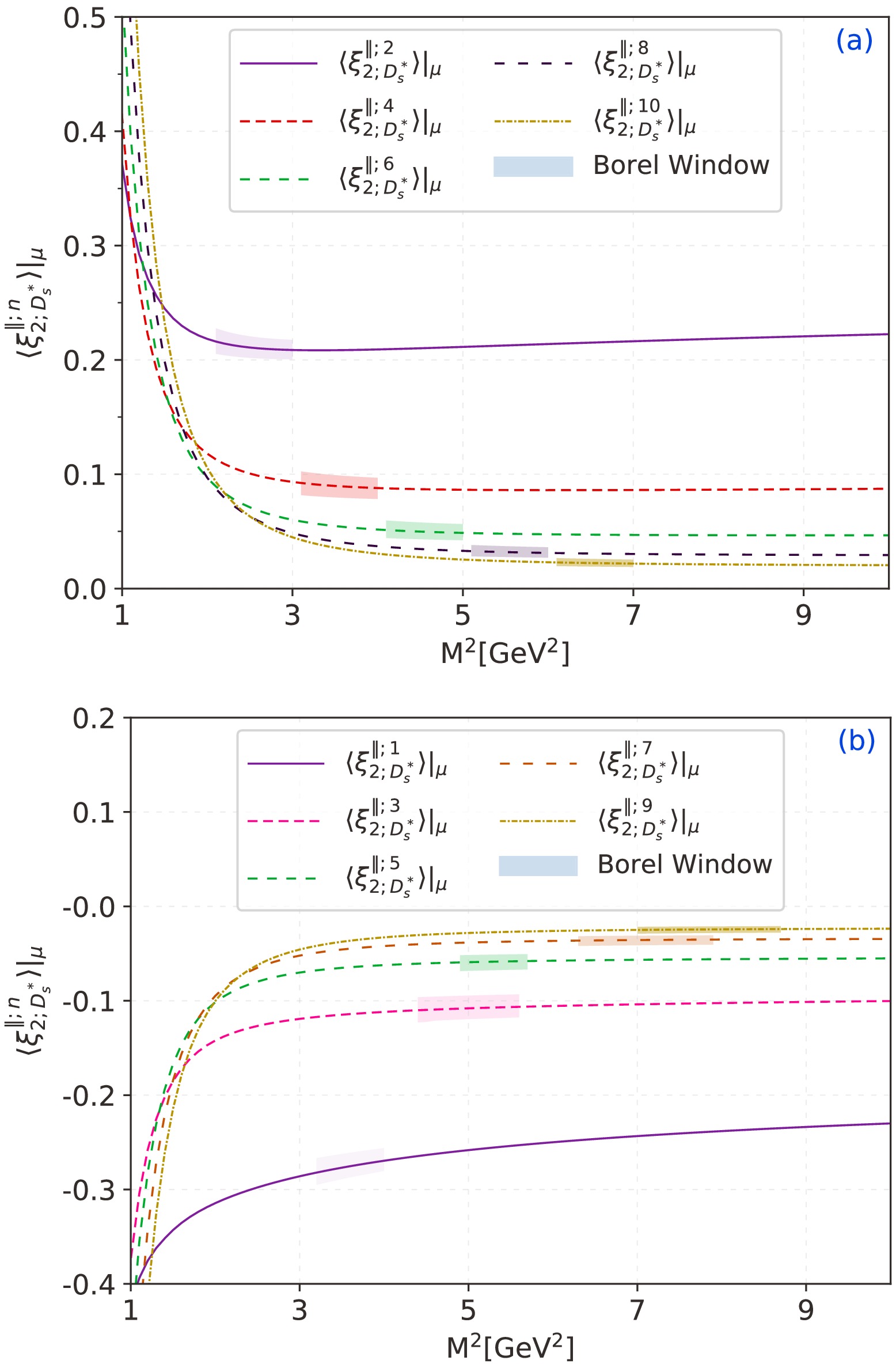

Figure 1.  (color online) $D_s^*$-meson twist-2 LCDA moments $\langle\xi^{\|;n}_{2;D_s^*}\rangle|_\mu$ with $(n=1,\cdots,10)$ versus the Borel parameter $M^2$. Here, we only present the central values to show the curves of different moments clearly.

	$ \mu_0=1.3~ \mathrm{GeV} $	$ \mu_k=3.0~ \mathrm{GeV} $
$ \langle\xi^{\|;1}_{2;D_s^*}\rangle|_\mu $	$ -0.302_{-0.046}^{+0.038} $	$ -0.258_{-0.039}^{+0.033} $
$ \langle\xi^{\|;2}_{2;D_s^*}\rangle|_\mu $	$ +0.229_{-0.034}^{+0.039} $	$ +0.179_{-0.026}^{+0.031} $
$ \langle\xi^{\|;3}_{2;D_s^*}\rangle|_\mu $	$ -0.121_{-0.019}^{+0.015} $	$ -0.104_{-0.016}^{+0.013} $
$ \langle\xi^{\|;4}_{2;D_s^*}\rangle|_\mu $	$ +0.101_{-0.014}^{+0.017} $	$ +0.083_{-0.012}^{+0.014} $
$ \langle\xi^{\|;5}_{2;D_s^*}\rangle|_\mu $	$ -0.066_{-0.010}^{+0.009} $	$ -0.057_{-0.009}^{+0.007} $
$ \langle\xi^{\|;6}_{2;D_s^*}\rangle|_\mu $	$ +0.053_{-0.007}^{+0.009} $	$ +0.045_{-0.006}^{+0.008} $
$ \langle\xi^{\|;7}_{2;D_s^*}\rangle|_\mu $	$ -0.041_{-0.007}^{+0.006} $	$ -0.035_{-0.006}^{+0.005} $
$ \langle\xi^{\|;8}_{2;D_s^*}\rangle|_\mu $	$ +0.037_{-0.005}^{+0.006} $	$ +0.031_{-0.004}^{+0.005} $
$ \langle\xi^{\|;9}_{2;D_s^*}\rangle|_\mu $	$ -0.026_{-0.004}^{+0.003} $	$ -0.023_{-0.004}^{+0.003} $
$ \langle\xi^{\|;10}_{2;D_s^*}\rangle|_\mu $	$ +0.025_{-0.004}^{+0.004} $	$ +0.022_{-0.003}^{+0.004} $

Table 1.  First tenth-order ξ-moments of $ D_s^* $-meson longitudinal twist-2 distribution amplitude $ \phi_{2;D_s^*}^\|(x,\mu ) $ at the scale $ \mu_0=1.3\ \mathrm{GeV} $ and $ \mu_k=3.0\ \mathrm{GeV} $.

Then, using the least squares method to fit the values of the ξ-moments in Table 1 with the LCHO model shown in Eq. (26), the behavior of the $ D_s^* $-meson longitudinal twist-2 LCDA $ \phi_{2;D_s^*}^\|(x,\mu) $ can be determined. Through the fitting method detailed in Refs. [55, 56], we determined the model parameters and corresponding goodness of fit. That is, by the magnitude of the probability $ P_{\chi_{\min}^{2}} = \int_{_{\chi_{\min}^{2}}}^{\infty}{f(y;n_d)}{\rm d}y $ with the probability density function of $ \chi^2(\theta) $, $ f(y;n_d) = \dfrac{1}{\Gamma(n_d/2) 2^{n_d/2}}y^{n_d/2-1}{\rm e}^{-y/2} $, one can intuitively judge the goodness of fit. Here, $ n_d $ represents the number of degrees of freedom. The optimal values of model parameters $ \alpha_{2;D_s^*} $, $ B_{1}^{2;D_s^*} $, and $ \beta_{2;D_s^*} $ at scale $ \mu_k = 3.0\; \mathrm{GeV} $ and their goodness of fit are as follows:

Subsequently, using the model parameters, we determined the behavior of the leading-twist longitudinal LCDA $ \phi_{2;D_s^*}^\|(x,\mu) $ of the $ D_s^* $-meson, as shown in Fig. 2. In the figure, we display the evolution of the leading-twist LCDA $ \phi_{2;D_s^*}^\|(x,\mu) $ of the $ D_s^* $-meson at different energy scales $ \mu = (3, 10, 30,100)\; {\rm{GeV}} $, including the asymptotic form. As the energy scale increases, the peak position of $ \phi_{2;D_s^*}^\|(x,\mu) $ gradually shifts towards $ x = 0.5 $, and the symmetry of the distribution improves; thus, it can be observed that, as $ \mu\to\infty $, the distribution shape of $ \phi_{2;D_s^*}^\|(x,\mu) $ gradually converges to the asymptotic form.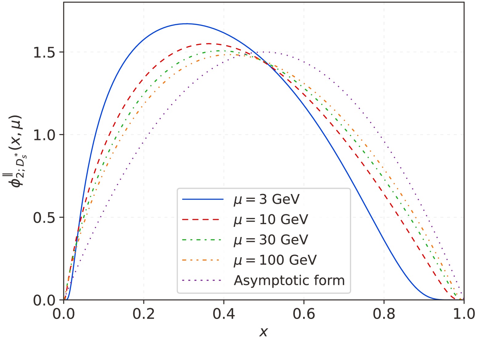

Figure 2.  (color online) Leading-twist light-cone distribution amplitude $\phi_{2;D_s^*}^\|(x,\mu)$ of the $D_s^*$-meson at different energy scales, incorporating the graphical description of the asymptotic form.

Based on the resultant $ D_s^* $-meson longitudinal leading-twist DA, we can then calculate the $ B_s\to D_s^* $ TFFs $ A_{1}(q^2) $, $ A_{2}(q^2) $, and $ V(q^2) $. The basic input parameters were mentioned at the beginning of this section. Therefore, the main task is to determine the continuum threshold parameter $ s_0 $ and Borel window $ M^2 $. Based on the basic idea and process of LCSR, we adopt the following four guidelines:

● the continuum contributions are less than 30% of the total results;

● the contributions from higher-twist DAs are less than 5%;

● within the Borel window, the changes of TFFs do not exceed 10%; and

● the continuum threshold $ s_0^{D_s^*} $ should be closer to the squared mass of the first excited state $ D_s^* $-meson.

Based on the above criteria, we determined the values of the continuum threshold $ s_0^{D_s^*} $ and Borel window $ M^2 $. According to the standard LCSR process, we calculate the final results of the TFFs and present them in Table 2. For comparison, we also give the results predicted by other theoretical groups CCQM [14], QCDSR [15], RQM [16], PQCD [18], and LFQM [19]. By comparison, we can see that our predicted results are in good agreement with those predicted by these theoretical groups within the error range.

	$ V(0) $	$ A_1(0) $	$ A_2(0) $
This work	$ 0.647_{-0.069}^{+0.076} $	$ 0.632_{-0.135}^{+0.228} $	$ 0.706_{-0.092}^{+0.109} $
CCQM [14]	$ 0.743\pm0.030 $	$ 0.681\pm0.065 $	$ 0.630\pm0.025 $
SR [15]	$ 0.63\pm0.05 $	$ 0.62\pm0.10 $	$ 0.75\pm0.07 $
RQM [16]	$ 0.95\pm0.02 $	$ 0.70\pm0.01 $	$ 0.75\pm0.02 $
PQCD [18]	$ 0.64\pm0.12 $	$ 0.50\pm0.09 $	$ 0.53\pm0.11 $
LFQM [19]	$ 0.74_{-0.05}^{+0.05} $	$ 0.61_{-0.04}^{+0.04} $	$ 0.59_{-0.04}^{+0.04} $

Table 2.  $ B_s\to D_s^* $ TFFs in large recoil region, i.e., $ A_{1}(0) $, $ A_{2}(0) $, and $ V(0) $, with uncertainties. Comparisons with theoretical groups are also given.

To access the information of $ B_s\to D_s^*\ell \bar\nu_{\ell} $ TFFs in the whole kinematic region, we must extrapolate the LCSR predictions obtained above towards large momentum transfer with a certain parametrization for the TFFs. The physically allowable ranges for the TFFs are $ 0 \leq q^2\leq q^2_{\rm{max}} = (m_{B_{s}} - m_{D_s^*})^2\sim10.6\; {\rm{GeV}}^2 $. Theoretically, the LCSR approach for $ B_s\to D_s^*\ell \bar\nu_{\ell} $ TFFs is in low and intermediate $ q^2 $-regions, i.e., $ 0 \leq q^2\leq 5\; {\rm{GeV}}^2 $ of $ D_s^* $-meson. One can extrapolate it to whole $ q^2 $-regions by rapidly $ z(q^2,t) $ converging the simplified series expansion (SSE), i.e., the TFFs are expanded as [57, 58]

where $ \beta_k $ are real coefficients and $ z(q^2,t) $ is the function

with $ t_{\pm} = (m_{B_s} \pm m_{D_s^{*}})^2 $ and the auxiliary parameter $ t_0 = t_{\pm}(1-\sqrt{1-t_-/t_+}) $. The SSE method possesses superior merit, which keeps the analytical structure correct in the complex plane and ensures the appropriate scaling, $ f_+(q^2)\sim 1/q^2 $, at large $ q^2 $. The quality of fit Δ is devoted to capturing the resultant extrapolation, which is defined as

After extrapolation for the TFFs $ A_{1}(q^2) $, $ A_{2}(q^2) $, and $ V(q^2) $ to the physical $ q^2 $-region, the behaviors of the $ B_s\to D_s^*\ell \bar\nu_{\ell} $ TFFs in the whole physical region can be obtained. These behaviors are shown in Fig. 3. For comparison, we also present the results predicted by other theoretical groups for the TFFs in detail.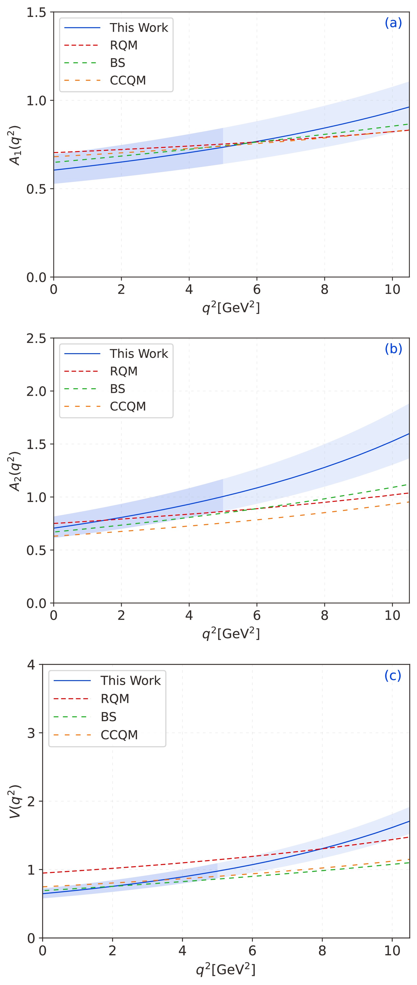

Figure 3.  (color online) Extrapolated TFFs $A_{1}(q^2)$, $A_{2}(q^2)$, and $V(q^2)$ versus $q^2$. The solid blue line is the central value, and the shaded band is the corresponding uncertainty. For comparison, the predictions under the RQM [16], BS [20], and CCQM [59] approaches are also presented.

● In Fig. 3, the lighter band represents the LCSR results of our prediction, while the darker band represents the SSE predictions.

● In the figure, the solid blue line represents this work. The red, green, and yellow dotted lines represent the results predicted by the RQM [16], CCQM [59], and Bethe-Salpeter (BS) [20] methods, respectively;

● To see the behavior of TFFs $ A_{1}(q^2) $, $ A_{2}(q^2) $, and $ V(q^2) $ more directly, as a comparison, we also show the predictions of theoretical groups such as RQM, CCQM, and BS. In comparison, our results are found to be consistent within the appropriate margin of error.

The differential branching ratio is a very important physical observable measurement of the semileptonic decay process, and its study helps us to understand the internal structure of particles and their interactions with other particles. Therefore, it is very important to calculate $ B_s\to D_s^*\ell \bar\nu_{\ell} $ semileptonic decay and its branching ratio. Here, we use $ |V_{cb}| = 0.041 $ to calculate [5], and using the branching ratio formula, we can obtain the numerical result of the branching ratio. In addition, we present the differential decay width diagram in Fig. 4. For comparison, we also show the predictions of other theoretical groups, including CCQM [14] and RQM [16]. We can see that our results agree well with both experimental and theoretical predictions within a suitable error range.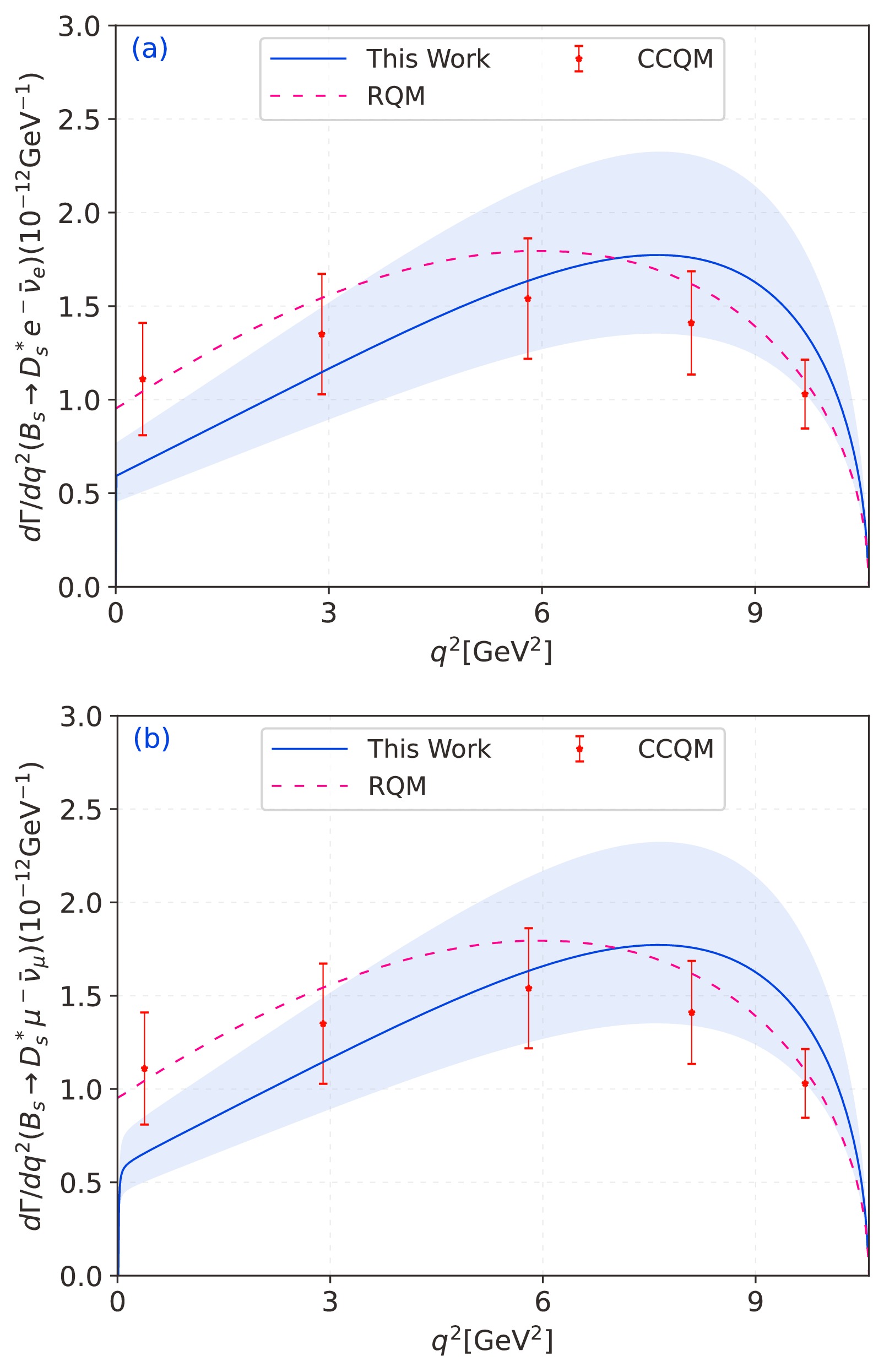

Figure 4.  (color online) Differential decay widthes for $B_s\to D_s^*\ell \bar\nu_{\ell}$ in whole $q^2$-region, where the solid line is the central value, and the shaded band shows its uncertainty. For comparison, this paper also introduces the use of different theoretical methods, such as CCQM [14] and RQM [16].

In Table 3, we comprehensively present the numerical results for the branching ratios of various decay channels associated with the semileptonic decay of $ B_s\to D_s^*\ell \bar\nu_{\ell} $. Alongside our findings, we showcase the numerical predictions offered by other leading theoretical groups, namely, CCQM [14], RQM [16], LFQM [19], PQCD [18], and PDG [5]. Upon conducting a meticulous comparison among these results, we notice that there exists a certain degree of deviation between our outcomes and those reported by the other groups. This discrepancy can likely be attributed to errors in the input parameters utilized in the respective calculations. Nevertheless, it is important to emphasize that, within a reasonable and acceptable range of error, our results are deemed to be valid and reliable.

Decay Channel	$ B_s^0\to {D_{s}^{*+}}e^-\nu_{e} $	$ B_s^0\to {D_{s}^{*+}}\mu^- \nu_\mu $
This Work	$ 5.45_{-1.57}^{+2.15} $	$ 5.43_{-1.57}^{+2.14} $
PDG [5]	-	$ 5.2\pm0.5 $
CCQM [14]	$ 6.42\pm0.67 $	$ 6.39\pm0.67 $
RQM [16]	$ 5.3\pm0.5 $	-
LFQM [19]	-	$ 5.2\pm0.6 $
PQCD [18]	$ 4.42_{-1.00}^{+1.27} $	-

Table 3.  Branching fractions (in unit: %) for the decays $ B_s^0 \to D_s^{*+}\ell \bar\nu_{\ell} $ with $ \ell = (e,\mu) $ in this work. Theoretical results are also given for comparison.

Finally, we present our prediction of $ V_{cb} $ in Table 4, along with the predictions from other groups, namely, PDG [5], BABAR [60], Belle [61], LCSR [62], LQCD [63], and HQCD [64]. By comparing our results with those of other groups, it can be seen that due to the differences in decay processes, the errors vary accordingly.

	$ |V_{cb}| $
This Work	$ 40.11_{-7.49}^{+6.54} $
PDG [5]	$ 41.4\pm1.3 $
BABAR [60]	$ 41.9\pm1.16 $
Belle [61]	$ 40.83\pm1.13 $
LCSR [62]	$ 40.2_{-0.5}^{+0.6}|_{th}\pm1.4|_{exp} $
LQCD [63]	$ 41.01\pm0.75 $
HPQCD [64]	$ 40.2\pm0.017\pm0.013 $

Table 4.  Our prediction of $ |V_{cb}| $ obtained from the decay channels $ B_s^0 \to D_s^{*+}\ell \bar\nu_{\ell} $, compared with other theoretical and experimental results of various channels (in unit $ 10^{-3} $).

This study investigated the semileptonic decay process of $ B_s\to D_s^*\ell \bar\nu_{\ell} $ within the framework of QCDSR. First, we presented expressions for the $ D_s^* $-meson longitudinal twist LCDA moments $ \langle \xi_{2;D_s^*}^{\|,n} \rangle|_\mu $ and listed the values of the first ten ξ-moments at $ \mu_0 = 1.3\; \mathrm{GeV} $ and $ \mu_k = 3.0\; \mathrm{GeV} $ (Table 1). Subsequently, we employed the least squares method to fit the values of the tenth-order ξ-moments at $ \mu_k = 3.0\; \mathrm{GeV} $ to determine the corresponding model parameters. Based on the BHL method, we constructed a new model of $ \phi_{2;D_s^*}^{\|}(x,\mu) $, whose behavior is constrained by normalization conditions, the probability of finding the leading Fock-state in the $ D_s^* $-meson Fock-state expansion, and known Gegenbauer moments. Research shows that it is necessary to find a more accurate form of meson DA. In the study of various processes, the error caused by using meson DA as an input parameter should be considered. To present the behavior of the LCDA $ \phi_{2;D_s^*}^{\|}(x,\mu) $ in a clear and intuitive manner, we depicted its curve in Fig. 2.

Then, we calculated $ B_s\to D_s^*\ell \bar\nu_{\ell} $ TFFs $ A_1(q^2) $, $ A_2(q^2) $, and $ V(q^2) $ using the LCSR method. We presented the numerical results of the TFFs in the large recoil region in Table 2. After extrapolating the LCSR results of $ B_s\to D_s^* $ TFFs to the entire $ q^2 $-region, the differential decay width and branching ratio of the semileptonic decay $ B_s\to D_s^*\ell \bar\nu_{\ell} $ were obtained, as shown in Table 3 and Fig. 4. The CKM matrix element $ |V_{cb}| $ calculated using the branching ratios obtained by the LHCb Collaboration is presented in Table 4. It was compared with other predictions and found to be consistent with experimental data and other methods within the error range.

We are grateful to Prof. Yu-Ming Wang and Prof. Bernard Pire for their valuable comments. Tao Zhong and Hai-Bing Fu would like to thank the Institute of High Energy Physics of Chinese Academy of Sciences for their warm and kind hospitality.