Searching for doubly charmed baryons from ${ \overline{\boldsymbol B}_{\boldsymbol c}}$ meson decays

The LHCb collaboration reported experimental evidence of the doubly charmed baryon candidate $ \Xi_{cc}^{++} $ in the $ \Lambda_c^+ K^- \pi^+\pi^+ $ final state in 2017 [1]. Its mass was determined to be $ 3621.55 $ MeV [2], and its lifetime, measured from weakly decays, was $ 0.256 $ ps [3]. Prior to this, the doubly charmed baryon $ \Xi_{cc}^+ $ with a mass of $ 3518.7 $ MeV was first reported by the SELEX collaboration in decay modes $ \Xi_{cc}^+\to \Lambda_c^+ K^- \pi^+ $ and $ \Xi_{cc}^+ \to p\, D^+ K^- $ [4, 5]; its lifetime was found to be less than 33 fs. However, subsequent experiments, namely FOCUS [6], BaBar [7], Belle [8], and LHCb [9], have not confirmed this state yet. Likewise, for $ \Omega_{cc}^+ $ baryons, the most recent searches from the LHCb collaboration have not reported a significant detection signal yet. Therefore, further theoretical and experimental efforts to advance the study of doubly heavy baryons are urgently needed.

This is crucial for completing the hadron spectrum and revealing the nature of perturbative and non-perturbative QCD dynamics related to doubly heavy baryons. Various theoretical frameworks, such as lattice QCD [10−14], quark model [15−22], QCD sum rules [23−28], and heavy baryon chiral perturbation theory [29−32], have been applied for research on doubly heavy systems. For ground states of $ \Xi_{cc} $, the majority of theoretical predictions focus on masses and lifetimes. For instance, the masses are predicted to lie in the range of 3.5−3.7 GeV, which is close to current experimental measurements. Owing to the effect of the destructive Pauli interference of the c quark decay products and valence u quark in the initial state, the lifetime of $ \Xi_{cc}^{++} $ is expected to be approximately 2−4 times larger than the one of $ \Xi_{cc}^+ $. Consequently, most theoretical predictions show that the lifetime of $ \Xi_{cc}^+ $ is in the range of 40−160 fs. There are also many theoretical predictions for the ground state of $ \Omega_{cc}^+ $; for instance, its mass is predicted to be approximately 3.6−3.9 GeV, and its lifetime is 75−180 fs. We provide some typical results in Table 1.

	LQCD [11]	QM [17]	[1]	QCDSR [24]	NR model [33]	OPE [34, 35]	Exp (mass & lifetime)
$\Xi^{++}_{cc}$	3.610 GeV	3.676 GeV	3.627 GeV	3.72 GeV	0.67 ps	0.52 ps	3.622 GeV [2]	0.256 ps [3]
$\Xi_{cc}^+$	3.610 GeV	3.676 GeV	3.627 GeV	3.72 GeV	0.25 ps	0.19 ps	3.519 GeV [5]	$<33$ fs [5]
$\Omega^+_{cc}$	3.738 GeV	3.832 GeV	−	3.73 GeV	0.21 ps	0.22 ps	−	−

Table 1.  Masses and lifetimes of doubly charmed baryons predicted from several theoretical methods or experiments.

Here, we present a new study about production of doubly charmed baryons from $ \overline B_c $ mesons. This production may be achieved by the LHCb and future b-factories. We derive the production processes using the effective Lagrangian method [36, 37]. The complete transition is divided into a weakly decay part associated with the transition $ {\cal{O}}^i:\ \bar b\to\bar c c\bar d/\bar s $ and a strongly coupled part related to two strong coupled vertices, i.e., $ {\cal{B}}_{cc}{\cal{B}}_cD $ and $ {\cal{B}}_{c}{\cal{B}}_{c}J/\psi $ ($ {\cal{B}} $ is the general baryon). The production can then be described formally by some triangle diagrams at the hadronic level. Under the $S U$(3) light quark flavor symmetry [38−44], it is convenient to relate different production channels, where the final states can include one doubly charmed baryon $ {\cal{B}}_{cc} $ ($ \Xi_{cc}^{++} $, $ \Xi_{cc}^+ $, $ \Omega_{cc}^+ $) and an anti-charmed triplet baryon $ {\cal{B}}_{\bar c3} $ or anti-sextet baryon $ {\cal{B}}_{\bar c\bar 6} $,

Furthermore, the rates of decay widths are related to the Cabibbo-Kobayashi-Maskawa (CKM) matrix elements $ V_{cs} $ and $ V_{cd} $,

and we calculate the branching ratio using the effective Lagrangian method. Thus, we can compare the results with the predictions from $S U$(3) analysis, aiming to provide assistance in understanding and searching for doubly heavy baryons.

The rest of this paper is organized as follows. In Sec. II, we introduce the calculation framework that describes the production of doubly charmed baryons from $ \overline B_c $ decays. Several amplitudes of triangle diagrams are obtained using the effective Lagrangian method. In Sec. III, we present numerical analyses and branching ratios of different processes. The final section provides a brief summary.

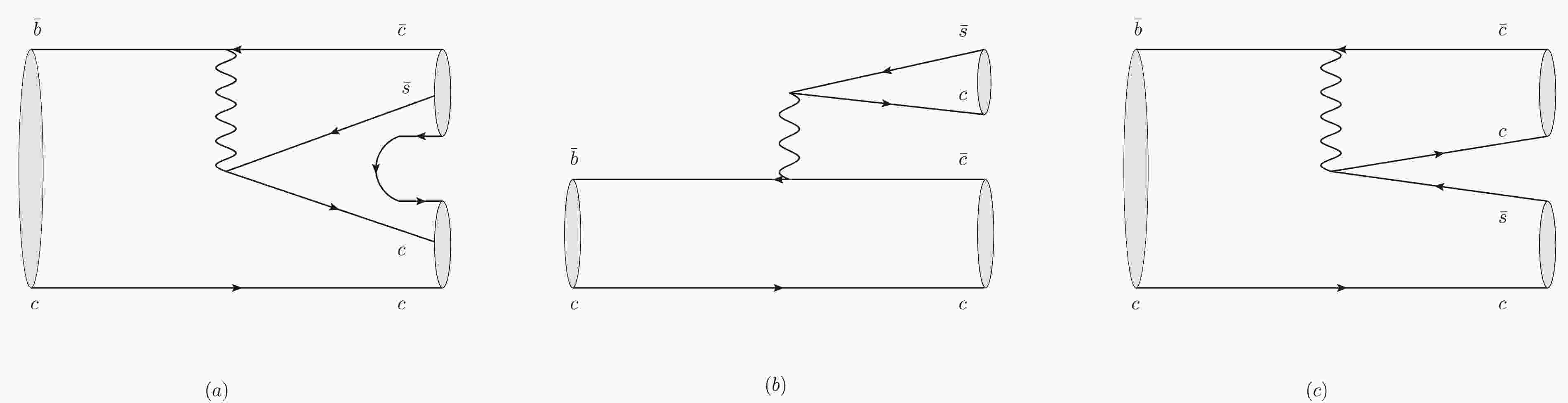
The production of doubly charmed baryons $ {\cal{B}}_{cc} $ from $ \overline B_c $ occurs through the weak decay of the bottom quark $ \bar b \to \bar c c \bar d/\bar s $, whose topological diagram at the quark level is shown in Fig. 1(a). The non-factorizable color suppressed diagram with two baryons in the final states is unusual and difficult to handle directly using common factorization schemes. In this paper, we consider the process within the framework of the effective Lagrangian approach—a convenient method for studying hadrons at the hadronic level. The total production matrix element can be further divided into a weak transition matrix and a strongly coupled matrix by inserting a complete basis,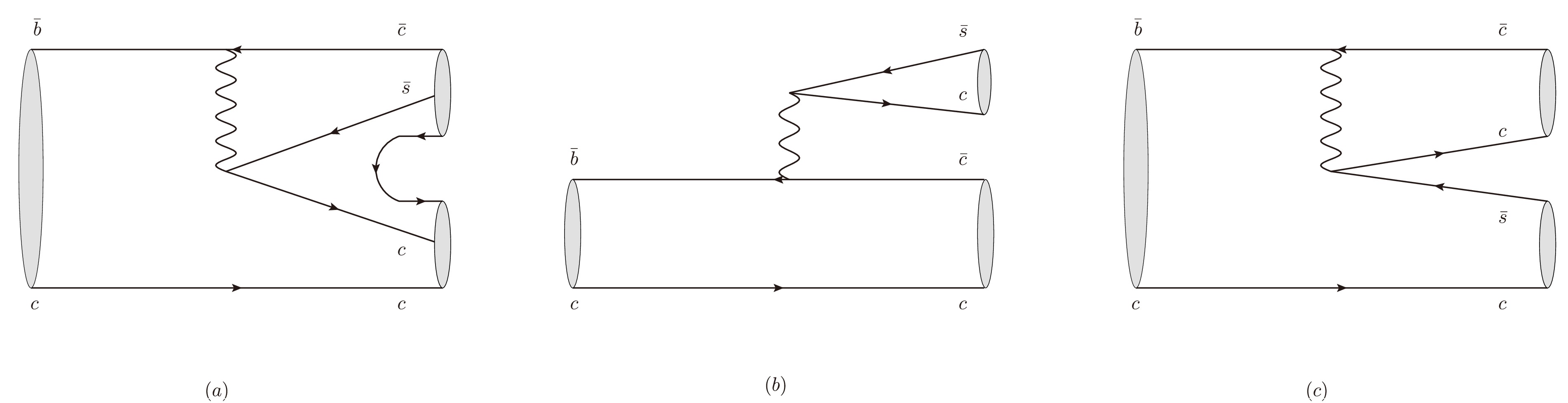

Figure 1.  (a) Production processes of $\overline B_c\to {\cal{B}}_{cc}+\overline {{\cal{B}}}_{\bar c}$, which are non-factorizable and color suppressed; (b) and (c) weak decays of $\overline B_c \to D(D^*)+J/\psi(\eta_c)$ in terms of the factorizable external and internal W-emission diagrams, respectively.

Here, $ H_{\lambda} $ denotes the strong interaction term included in the interaction representation presented later. It is clear that the dominant contribution related to the weak transition matrix corresponds to $ \langle D(D^*)\eta_c|{\cal{H}}_{\rm eff}|\overline B_c\rangle $ or $ \langle D(D^*)J/\psi|{\cal{H}}_{\rm eff}|\overline B_c\rangle $ (here, we only consider the major contribution $ \lambda = D(D^*)J/\psi(\eta_c) $), which is depicted as an accessible emission diagram [45] in Figs. 1(b) and (c). Meanwhile, the remaining one can be decoded using several effective Lagrangians introduced below. Combining them, we obtain productions of spin-$ \frac{1}{2} $ doubly charmed baryons $ {\cal{B}}_{cc} $ ($ \Xi_{cc}^{++},\Xi_{cc}^+,\Omega_{cc}^+ $) resulting from the triangle diagrams. We proceed with processes under the quark transition $ \bar b\to \bar c c\bar s $,

and under the transition $ \bar b\to \bar c c \bar d $,

The corresponding triangle diagrams are shown in Fig. 2. Here, we have excluded some unallowable processes in the phase space as well as processes with decoupling vertices.

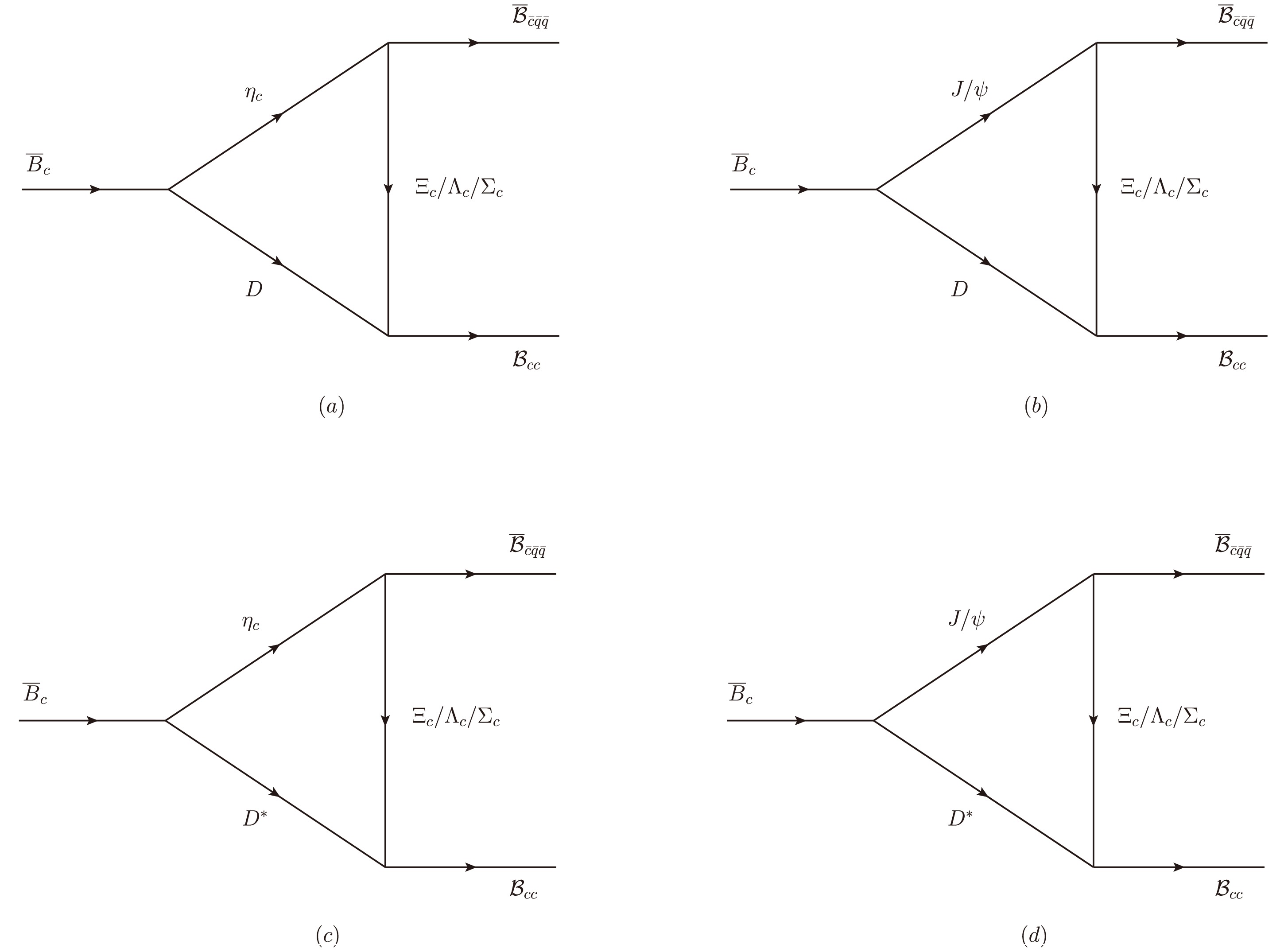
Figure 2.  Triangle diagrams attached to the production of doubly charmed baryons, mediated by the exchange of charm baryons $\Xi_c,\Lambda_c,\Sigma_c$.

We adopt the effective Lagrangian to study the production of doubly charmed baryons. The process can be regarded as $ \overline B_c $ mesons first decaying into $ D(D^*) $ and $ J/\psi\,(\eta_c) $mesons and then exchanging with charm baryons $ {\cal{B}}_c $ to produce anti-charmed baryons $ \overline{{\cal{B}}}_{\bar c} $ and doubly charmed baryons $ {\cal{B}}_{cc} $, $ \overline B_c \to M_1M_2 \xrightarrow[]{{\cal{B}}_c} \overline{{\cal{B}}}_{\bar c}{\cal{B}}_{cc} $ ($ M_1M_2 $ can be $ J/\psi \,D,~\eta_c \,D,~J/\psi \,D^* $, or $ \eta \,D^* $). The weak decay $ \overline B_c \to J/\psi \,(\eta_c)+ D \,(D^*) $ can occur via the factorizable W-emission process shown in Fig. 1(b). It typically provides the largest contribution according to the topological classification of weak decays. The effective Hamiltonian is

where $ G_F $ is the Fermi constant, $ C_{1,2}(\mu) $ denotes the Wilson coefficients, and $ {\cal{O}}_{1,2}(\mu) $ denotes the tree level fermion operators, with $ {\cal{O}}_{1} = (\bar b_{\alpha} c_{\beta})_{V-A}(\bar c_{\beta}s_{\alpha})_{V-A} $ and $ {\cal{O}}_{2} = (\bar b_{\alpha} c_{\alpha})_{V-A} (\bar c_{\beta}s_{\beta})_{V-A} $. The combinations of the effective Wilson coefficient $ a_{1,2} $ are $ a_1 = C_1+C_2/N_c $ and $ a_2 = C_2+C_1/N_c $, where $ N_c $ denotes the number of colors.

The amplitude of the weak process can be expressed as the product of two current hadronic matrix elements, accompanied by form factors and decay constants,

The matrix elements between pseudoscalar or vector mesons and vacuum have the following formations [46]:

where P and V stand for pseudoscalar and vector mesons, respectively; $ f_{P} $ and $ f_{V} $ are the pseudoscalar and vector meson decay constants, respectively; and $ \varepsilon^*_{\mu} $ represents the polarization vector of the vector meson.

We follow the parameterized form of the transition $ \overline B_c \to J/\psi D \,(D^*) $ [47],

where $ \varepsilon_{\mu} $ denotes the polarization vector of $ J/\psi $, and the transition momentum satisfies $ q_{\mu}\equiv(P_{B_c}-P_P)_{\mu} $. To cancel the poles at $ q^2 = 0 $, invariant weak form factors $ F_0(q^2),\, F_1(q^2),\, A_0(q^2) $, and $ A_3(q^2) $ satisfy the following conditions:

In the $ S U$(4) symmetry, the interaction Lagrangians related to the processes are expressed as [48]

Here, $ g_{{\cal{B}}{\cal{B}}P} $ and $ g_{{\cal{B}}{\cal{B}}V} $ are the couplings of the pseudoscalar meson or vector meson and two baryons $ {\cal{B}}{\cal{B}} $. Given that there are no experimental data to extract values for the needed couplings, we deduce them from the generic $S U $(4) symmetry, i.e., we use the empirical values $g_{NN\pi} = 13.5(5),\, g_{\rho NN} = 3.25(90),\, f_{\rho NN} = \kappa_{\rho} g_{\rho NN},\, \kappa_{\rho} = 6.1(1)$ [49, 50] to obtain the couplings between doubly charmed and charmed baryons. For more details, please refer to Appendix A. Within $S U$(4) symmetry, pseudoscalar and vector mesons are reclassified as 15-plet, whose expressions are [51]

and

Baryons represented as $ {\cal{B}} $ belong to a 20-plet,

These states are expressed by tensors $ {\cal{B}}^{{\rm i}jk} $, where the first two indices are anti-symmetric.

With the effective Lagrangians at hand, we can obtain the decay amplitudes shown in Fig. 2. For instance, the amplitude of $ \overline B_c\to \Xi_{cc}^{++}\overline \Xi_{\bar c}^- $ is

where $ k_3 = p_1+k_1 $ is the momentum of $ J/\psi \,(\eta_c) $, and $ k_2 = p_2-k_1 $ is the momentum of $ D\,(D^*) $, respectively. Hadrons have finite sizes; therefore, the monopole form factor is adopted at each vertex,

where Λ is the so-called cutoff mass, which governs the range of suppression. We use the expression $ \Lambda = m_{E}+\alpha $ [39], where $ m_E $ is the mass of the exchanged particle and $ \alpha = \eta \Lambda_{\rm QCD} $. Usually the parameter η is expected to be of order unity and depends not only on the exchanged particle but also on the external particles involved in the strong-interaction vertex. In principle, it cannot be determined from first-principles calculations. However, we can set the parameter using the measured decay rates. In this $ B_c $ meson system [52], we take a naive value for α in the range of 100−300 MeV. The decay rate for the nonleptonic transition $ \overline{B}_c\to P_1P_2 $ is expressed in terms of the decay amplitude $ {\cal{M}}(\overline{B}_c\to P_1P_2) $

where $ {{\bf{P}}_{\bf{1}}} $is the magnitude of the three momenta of the final state meson, expressed as $ |{{\bf{P}}_{\bf{1}}}| = \dfrac{1}{2m_{B_c}} $ $ \sqrt{\lambda(m_{B_c}^2,m^2_{{\cal{B}}_{cc}},m^2_{\overline {{\cal{B}}}_{\bar c}})} $; $ \lambda(a,b,c) = a^2+b^2+c^2- 2ab-2bc-2ac $.

The calculation of branching ratios requires the following decay constants of several pseudoscalar and vector mesons:

Furthermore, the masses of mesons and baryons are extracted from PDG [53]. Numerous strong couplings are deduced from $ S U$(4) symmetry (see Appendix A).

In the physical region, each of the transition form factors can be accurately interpolated using the following function [54]:

where the parameters $ \alpha_{1,2,3} $ are taken from Table 2.

	$\overline B_c\to \eta_c$			$\overline B_c\to J/\psi$
	$F_1(0)$	$F_0(0)$		$V_0(0)$	$A_0(0)$	$A_1(0)$	$A_2(0)$	$A_3(0)$
$\alpha_1$	0.632(13)	0.632(13)		0.836(41)	0.574(33)	0.551(25)	0.561(28)	0.574(33)
$\alpha_2$	0.032(24)	0.025(11)		0.045(80)	0.030(43)	0.018(38)	0.021(35)	0.030(43)
$\alpha_3$	0.061(13)	0.034(7)		0.028(110)	0.055(25)	0.036(61)	0.037(77)	0.055(25)

Table 2.  Interpolation parameters of form factors in Eq. (10); $\alpha_1$ is dimensionless, and $\alpha_{2,3}$ have dimensions of GeV$^{-1}$.

Using these expressions and results, we can determine the production of doubly charmed baryons from $ \overline B_c $ mesons, obtaining the number of widths and branching ratios presented in Table 3. Note that the branching ratio can reach values on the order of $ 10^{-5} $. In our analysis, we set the parameter $ \alpha = \Lambda_{\rm QCD} $ in Λ with a value of 250 MeV [55]. For completeness, the branching ratios as a function of α are presented in Fig. 3. Moreover, we verify the dominant sub-process of productions $ \overline {B}_c\to M_1 M_2 \xrightarrow[]{EP} \overline {{\cal{B}}}_{\bar c} \, {\cal{B}}_{cc} $ ($ M_1M_2 $ = $ J/\psi D,\, \eta_c D,\, J/\psi D^* $ or $ \eta D^* $). Based on the results, we draw several conclusions as follows.

Process	EP	Decay width ($\times 10^{-19}$)	Branching ratio ($\times 10^{-6}$)	Dominant $M_1M_2$
$\overline B_c \to \Xi_{cc}^{++} \overline \Xi_{\bar c}^-$	$\Xi_c$	$4.88^{+1.07}_{-0.92}$	$3.78^{+0.83}_{-0.71}$	$\eta_cD^*$
$\overline B_c \to \Xi_{cc}^+ \overline \Xi_{\bar c}^0 $	$\Xi_c$	$5.51^{+1.27}_{-1.06}$	$4.27^{+0.98}_{-0.82}$	$ \eta_cD^*$
$\overline B_c \to \Xi_{cc}^{++} \overline \Xi_{\bar c}^{'-}$	$\Xi_c^{'}$	$83.1^{+20.1}_{-17.3}$	$64.4^{+15.6}_{-13.4}$	$J/\psi D, \eta_c D^*$
$\overline B_c \to \Xi_{cc}^+ \overline \Xi_{\bar c}^{'0} $	$\Xi_c^{'}$	$117.9^{+29.2}_{-24.5}$	$91.4^{+22.6}_{-19.0}$	$J/\psi D, \eta_c D^*$
$\overline B_c \to \Xi_{cc}^{++} \overline \Lambda_{\bar c}^-$	$\Lambda_c$	$0.30^{+0.08}_{-0.07}$	$0.23^{+0.06}_{-0.05}$	$\eta_cD^*$
$\overline B_c \to \Xi_{cc}^+ \overline \Sigma_{\bar c}^0 $	$\Sigma_c$	$11.9^{+3.29}_{-2.72}$	$9.25^{+2.55}_{-2.11}$	$J/\psi D,\eta_cD^*$
$\overline B_c \to \Xi_{cc}^{++} \overline \Sigma_{\bar c}^-$	$\Sigma_c$	$5.37^{+1.50}_{-1.23}$	$4.16^{+1.16}_{-0.95}$	$J/\psi D, \eta_cD^*$
$\overline B_c \to \Omega_{cc}^+ \overline \Xi_{\bar c}^0 $	$\Xi_c$	$0.13^{+0.04}_{-0.03}$	$0.10^{+0.03}_{-0.02}$	$\eta_cD^*$

Table 3.  Branching ratios of doubly charmed baryons from $\overline{B}_c$ ($\overline{B}_c\to M_1 M_2 \xrightarrow[]{EP}\overline {{\cal{B}}}_{\bar c} \, {\cal{B}}_{cc}$) with $\Lambda=m_{{\cal{B}}_{c}}+0.25$ GeV. The exchanged particles (EP) can be $\Lambda_c,\Xi_c, \Sigma_c$. The dominant contribution from $M_1M_2$ are also presented.

Figure 3.  (color online) Branching ratios as a function of α in Λ; α varies in the range of 100−300 MeV. The left image contains four Cabibbo allowed processes, whereas the right one shows Cabibbo suppressed processes with transition $\bar b\to \bar cc \bar d$.

● Our calculations show that the production $ \overline B_c \to \Xi_{cc}^{++} \overline \Xi_{\bar c}^{'-} $ occupies the largest branching ratio among the processes considered in this study; this must be confirmed experimentally. Once verified, it could be an ideal candidate to produce doubly charmed baryons in the future. The dominant amplitude contribution comes from the sub-processes $ \overline {B}_c\to J/\psi D \xrightarrow[]{\Xi_c}\Xi_{cc}^{++} \overline \Xi_{\bar c}^{'-} $ (the branching ratio of this subprocess is $ 2.1\times 10^{-5} $) and $ \overline {B}_c\to \eta_c D^* \xrightarrow[]{\Xi_c} \Xi_{cc}^{++} \overline \Xi_{\bar c}^{'-} $ (the branching ratio of this subprocess is $ 1.1\times 10^{-5}) $. Therefore, the major contribution of branching ratios comes from these two sub-processes and their cross ones.

● It seems that the leading contributions of strong couplings are subprocesses with $ {\cal{B}}{\cal{B}}V $ or $ {\cal{B}}{\cal{B}}P $ vertices consistent with the processes, i.e, for $ \overline B_c \to \Xi_{cc}^{++} \overline \Xi_{\bar c}^{'-} $, the isolated contribution from a pair of $ {\cal{B}}{\cal{B}}P $ or $ {\cal{B}}{\cal{B}}V $ is trivial, merely on the order of $ 10^{-8} $.

● Unlike the first four Cabibbo allowed processes, the last four processes are Cabibbo suppressed. However, the branching ratios are still considerable. Especially, the undiscovered $ \Omega_{cc} $ can reach values on the order of $ 10^{-6} $.

● Table 3 shows the rates of decay widths: $ \Gamma(\overline B_c \to \Xi_{cc}^{++} \overline \Xi_{\bar c}^{-})/\Gamma(\overline B_c \to \Xi_{cc}^{++} \overline \Lambda_{\bar c}^{-}) \approx 16.4 $, $ \Gamma(\overline B_c \to \Xi_{cc}^{++} \overline \Xi_{\bar c}^{'-})/ \Gamma(\overline B_c \to \Xi_{cc}^{++} \overline \Sigma_{\bar c}^{-}) \approx 15.5 $; these values are consistent with the straightforward symmetry analysis expressed by Eq. (2), resulting in $ |V_{cs}|^2/|V_{cd}|^2 \approx 19.9 $. This confirms that the $ S U$(3) symmetry is basically maintained in these processes.

● According to a systematic error analysis that encompasses the uncertainties of form factors, decay constants, and coupling constants, the deviation of the central value can reach 20%. Further analysis reveals that the main uncertainties come from the coupling constant $ {\cal{B}}{\cal{B}}V $, i.e., $ g_{\rho NN} = 3.25(90) $, $ g_{\Xi_{cc}^+ \Sigma_{c} D^*} = -4.60(113) $; once these are excluded, the error will be less than 10%.

● The decay channels $ \overline {B}_c \to \overline {{\cal{B}}}_{\bar c} \, {\cal{B}}_{cc} $ have been calculated for the first time in this study. Previous studies reported the branching ratios for processes such as $ \bar{B}^0 \to \Lambda_c^+ + \bar{p} $ in the framework of perturbative QCD (pQCD) [56]; the effective operator involved, $ \bar b\to \bar c\bar u d $, is similar to ours, $ \bar b\to \bar cc\bar s $. However, it is well established that complete theoretical predictions within factorization schemes require non-perturbative inputs. In the present case, the wave functions of doubly charmed baryons remain unavailable, as there are currently no theoretical or experimental studies on their LCDAs. Consequently, we adopt the effective Lagrangian approach, which circumvents the need for explicit knowledge of hadronic LCDAs.

The observation of $ \Xi_{cc}^{++} $ by the LHCb Collaboration has opened a new field of research on the nature of baryons containing two heavy quarks. Doubly charmed baryons can form an $S U$(3) triplet, $ \Xi_{cc}^{++}, \Xi_{cc}^{+} $, and $ \Omega_{cc}^+ $. Therefore, after the experimental observation of $ \Xi_{cc}^{++} $, it is of prime importance to search for additional production modes of this particle and the other two. It is worth noting that the charmonium pentaquarks were discovered from B-meson decays [57, 58]. This inspired us to search for doubly charmed baryons through meson decays.

In this paper, we have presented a theoretical study on the production of doubly charmed baryons from $ \overline B_c $ meson decays. The decay widths and branching ratios have been obtained using the effective Lagrangian method; the results are summarized in Table 3. We expect these results to be helpful for exploring new decay modes in the future.

The Lagrangian of $ {{\cal{B}}}{\cal{B}}P $ in $S U$(3) symmetry can be expressed as

where $ a_1 = D+F $, $ a_2 = D-F $, and $ \dfrac{D}{D+F} = \alpha_D = 0.64 $ [59]. Expanding the Lagrangian, we take the couplings of $ NN\pi $ and $ K\Lambda N $, and the rate is

Furthermore, the Lagrangian of $ {\cal{B}}{\cal{B}}P $ in $ S U$(4) symmetry is

Here, we show two equivalent tensor representations of baryons, $ {\cal{B}}^i_{[\alpha\beta]} \varepsilon^{jk\alpha\beta} $ and $ {\cal{B}}^{\{ij\}k} $, where $ [] $ and $ \{\} $ represent symmetric and anti-symmetric indices, respectively; $ \varepsilon^{jk\alpha\beta} $ is the total antisymmetric tensor. Expanding the Lagrangian, we obtain

Comparing the results in Eqs. (A2) and (A4), we have

This is similar for the case of $ {\cal{B}}{\cal{B}}V $ couplings. Generally, the Lagrangian of $ {\cal{B}}{\cal{B}}V $ in $S U$(3) symmetry can be expressed as

Expanding the Lagrangian and comparing the coupling $ \rho NN $ with $ K^* \Lambda N $, we obtain

The Lagrangian of $ BBV $in $S U$(4) symmetry is given below,

We again show two equivalent formulas. Similarly, one can obtain

and finally, we have

According to the couplings $ g_{NN\pi} = 13.5(5),\, g_{\rho NN} = 3.25(90),\, \kappa_{\rho} = 6.1(1) $ as well as the relations given in Eqs. (A5) and (A10), we can determine the required couplings: