


 Abstract
 HTML
HTML Reference
 Related
 PDF
PDF


-
The black hole singularity predicted by Einstein's theory is one of the main problems of general relativity. Different regular black hole solutions have been reported in the literature, e.g., the regular Bardeen black hole and charged black hole obtained from T-duality [1, 2] as well as black holes obtained in noncommutative geometry [3–5]. Such solutions are described by regular geometry, and the singularity predicted by classical general relativity is removed. In particular, one of the key concept used is the T-duality, which basically identifies string theories on higher-dimensional spacetimes with mutually inverse compactification radii R. The replacement rules are denoted as
$ R \rightarrow {R^\star}^2/R $ and$ n \leftrightarrow w $ , where$ R^\star = \sqrt{\alpha'} $ is known as the self-dual radius; in addition,$ \alpha' $ represents the Regge slope, n represents the Kaluza-Klein excitation, and w denotes the winding number [3–5]. As reported by Padmanabhan [6, 7], using the concept of T-duality, one can find the propagator that encodes string effects. This leads to modified gravitational and electric potentials [1, 2, 8]. Meanwhile, the Einstein-Gauss-Bonnet theory is known to be topological in$ 4D $ given that the Lagrangian in this theory is a total derivative and, as a result, it does not contribute to the gravitational dynamics. Therefore, we expect a non-trivial contribution when$ D \geq 5 $ . The problem of the EGB theory in 4D was addressed by Glavan & Lin [9] with the main objective of rescaling the Gauss-Bonnet coupling constant α as$ \alpha/(D -4) $ . After taking the limit$ D \to 4 $ , it was shown that a non-trivial gravitational dynamics is recovered. Interestingly, it was also shown that a regularized 4D theory at the level of action exists as a special case of the 4D Horndeski theory [10, 11]. Regarding the static and spherically symmetric black hole solutions, it was demonstrated that the regularized solution (obtained by rescaling the coupling constant) coincides with the original solution obtained by [9]. In the present study, we aimed to further understand possible exact black hole solutions in the 4D EGB theory inspired by the concept of T-duality.This paper is organized as follows. In Sec. II, we obtain a charged black hole solution in the string T-duality using the method proposed by Glavan & Lin [9]. In Sec. III, we obtain the same solution using a regularized method. In Sec. IV, we point out a connection with the GUP principle. In Sec. V, we study thermodynamics. Finally, in Sec. VI, we elaborate on our results.
-
Let us start by the momentum space propagator induced by the path integral duality (for the massless case), which is expressed as [1]
$G(k)= -\frac{ { {l_{{{0}}}} }}{\sqrt{k^2}}\, K_1 \left( { {l_{{{0}}}} } \sqrt{k^2}\right), $

(1) where
$ { {l_{{{0}}}} } $ denotes the zero-point length of spacetime and$ K_1 \left(x\right) $ is a modified Bessel function of the second kind. We have two special cases. First, at small momenta, i.e,. for$ {({ {l_{{{0}}}} } k)}^2 \to 0 $ , we have the conventional massless propagator:$ \begin{array}{*{20}{l}} G(k) = -k^{-2},\,\,\,\,\,\,\,\,\text{if}\,\,\,\,\,k^2 \ll 1/ { {l_{{{0}}}} }^2. \end{array} $

(2) For large momenta, we have the following expression:
$ \begin{array}{*{20}{l}} G(k) \sim - { {l_{{{0}}}} }^{1/2}\, {\left(k^2\right)}^{-3/4}\, {\rm e}^{- { {l_{{{0}}}} } \sqrt{k^2}},~~\text{if}~~ k^2 \gg 1/ { {l_{{{0}}}} }^2. \end{array} $

(3) We can obtain the potential corresponding to the virtual-particle exchange via path integral of the force-mediating field. It was shown that for the potential of the system, which consists of two pointlike masses, i.e., m and M, at relative distance
$ \vec{r} $ , one can write [1]$ \begin{align} \phi(r) \to -\frac{M}{\sqrt{r^2 + { {l_{{{0}}}} }^2}}. \end{align} $

(4) To generate a new solution that includes the electric charge, we must consider the energy contribution of the electric field encoded in the electromagnetic field given by [2, 8]
$ \begin{eqnarray} V(r)=-\frac{Q}{\sqrt{r^2+l_0^2}}. \end{eqnarray} $

(5) Next, we can write the general action in EGB gravity in D-dimensions:
$ S=\frac{1}{16 \pi}\int d^{D}x\sqrt{-g}\left[R+\frac{\alpha}{D-4} \mathcal{L}_{\text{GB}} \right]+S_{\text{matter}}, $

(6) where g is the determinant of the metric,
$ g=\det g_{\mu\nu} $ , and α is the Gauss-Bonnet coupling constant. We assume that a physically acceptable solution has to be non-negative, i.e.,$ \alpha \ge 0 $ . Furthermore,$ \mathcal{L}_{\text{GB}} $ is the Lagrangian in GB gravity given by$ \begin{array}{*{20}{l}} \mathcal{L}_{\text{GB}}=R^{\mu\nu\rho\sigma} R_{\mu\nu\rho\sigma}- 4 R^{\mu\nu}R_{\mu\nu}+ R^2 . \end{array} $

(7) where
$ S_{\text{matter}} $ corresponds to the matter fields appearing in the theory. If we now vary the action expressed by Eq. (6) with respect to metric$ g_{\mu \nu} $ , we obtain [9]$ G_{\mu\nu}+\frac{\alpha}{D-4} H_{\mu\nu}= 8 \pi { \mathfrak{T} }_{\mu \nu}. $

(8) In the present study, we also included the cosmological constant. However, we added the term on the right hand side of the Einstein field equations as part of the energy-momentum tensor. Thus, the total contribution is given by the quantum corrected term, the electromagnetic field, and the cosmological constant:
$ \begin{eqnarray} { \mathfrak{T} }_{\mu \nu}=T^{\rm str}_{\mu\nu}+T^{\rm em}_{\mu\nu}+T^{\rm vac}_{\mu\nu} \end{eqnarray} $

(9) along with
$ \begin{aligned}[b] G_{\mu\nu}=&R_{\mu\nu}-\frac{1}{2}R g_{\mu\nu},\\ H_{\mu\nu}=&2\Bigr( R R_{\mu\nu}-2R_{\mu\sigma} {R}{^\sigma}_{\nu} -2 R_{\mu\sigma\nu\rho}{R}^{\sigma\rho} - R_{\mu\sigma\rho\delta}{R}^{\sigma\rho\delta}{_\nu}\Bigl)\\ &-\frac{1}{2}\mathcal{L}_{\text{GB}}g_{\mu\nu}, \end{aligned} $

(10) where R is the Ricci scalar,
$ R_{\mu\nu} $ is the Ricci tensor,$ H_{\mu\nu} $ is known as the Lancoz tensor, and$ R_{\mu\sigma\nu\rho} $ is the Riemann tensor. The objective is to scale the coupling constant as$ \alpha/(D-4) $ ; by considering maximally symmetric spacetimes with curvature scale$ {\cal K} $ , we obtain [9]$ \frac{g_{\mu\sigma}}{\sqrt{-g}} \frac{\delta \mathcal{L}_{\text{GB}}}{\delta g_{\nu\sigma}} = \frac{\alpha (D-2) (D-3)}{2(D-1)} {\cal K}^2 \delta_{\mu}^{\nu}. $

(11) Note from Eq. (11) that the variation of the GB action does not vanish for
$ D=4 $ owing to the re-scaled coupling constant, which is the main concept in this method [9]. The first contribution is due to the string quantum corrected tensor:$ \begin{eqnarray} T^{\rm str}_{\mu \nu}=-\frac{2}{\sqrt{-g}}\frac{\delta \left(\sqrt{-g} \mathcal{L}\right)}{\delta g^{\mu \nu}}. \end{eqnarray} $

(12) The simplest choice is to take
$\mathcal{L}=-\rho^{\rm str}$ , where the energy density of the modified matter can be obtained by using the Poisson equation as follows [1]:$ \rho^{\rm str}(r)= \frac{3 { {l_{{{0}}}} }^2 M}{4 \pi {\left(r^2 + { {l_{{{0}}}} }^2\right)}^{5/2}}. $

(13) Concerning the energy-momentum of the vacuum, we have
$ \begin{eqnarray} T^{\rm vac}_{\mu\nu}=-\frac{\Lambda}{8\pi}\,\,\,g_{\mu \nu}. \end{eqnarray} $

(14) This has the form of a perfect fluid with
$ \rho^{\rm vac}=-p^{\rm vac}=\frac{\Lambda}{8 \pi}. $

(15) We will assume that the form of the energy-tensor of the electromagnetic field is
$ T_{\mu \nu}^{\rm em}=\frac{1}{4 \pi}\left(F_{\mu \sigma}{F_{\nu}}^{\sigma} -\frac{1}{4}g_{\mu \nu}F_{\rho \sigma}F^{\rho \sigma}\right), $

(16) where
$ F_{\mu\nu}=\nabla_\mu A_{\nu}-\nabla_\nu A_{\mu} $ . Finally, from the total energy momentum, we can write${({ \mathfrak{T} }^\mu}_\nu) = { \text{diag} }\left(-\rho^{\rm tot}, { {p_{r}} }, { {p_{t}} }, { {p_{t}} }\right)$ . Here,${ {p_{r}} }$ and${ {p_{t}} }$ are the radial and transverse pressures, respectively, and the total density is expressed as$\rho^{\rm tot}(r)=\rho^{\rm str}(r)+\rho^{\rm em}(r)+ \rho^{\rm vac}(r).$ The general solution in case of a static, spherically symmetric source reads$ {\rm d} s^2 = -f(r) {\rm d}t^2 +\frac{ {\rm d}r^2}{f(r)} +r^2({\rm d}\theta^2+\sin^2\theta {\rm d}\varphi^2). $

(17) For the
$ r-r $ and$ t-t $ components of the Einsteins field equations, we obtain (see also for example [12])$ -\frac{f'(r)}{r f(r)}+\frac{f^2(r)\alpha+(r^2-2 \alpha)f(r)-r^2+\alpha+8 \pi \rho r^4 }{r^2 f(r) (2 \alpha f(r)-r^2-2 \alpha)}=0, $

(18) $ \frac{f'(r)}{r f(r)}+\frac{f^2(r)\alpha+(r^2-2 \alpha)f(r)-r^2+\alpha-8 \pi \rho r^4 }{r^2 f(r) (-2 \alpha f(r)+r^2+2 \alpha)}=0 . $

(19) Note that the spherical symmetry existing in the spacetime metric imposes only non-vanishing components for the Faraday tensor [2]:
$ F_{tr}=-F_{rt}=-\frac{Q\, r}{\left(r^2+l_0^2\right)^{3/2}}, $

(20) and the energy density of the energy-momentum field and pressure components are respectively [2]
$ {\rho}^{\rm em}(r)=-{p_r}^{\rm em}(r)=\frac{Q^2 r^2}{8 \pi (r^2+l_0^2)^3} , $

(21) $ {p_t}^{\rm em}(r)=\frac{Q^2 r^2}{8 \pi (r^2+l_0^2)^3} . $

(22) Then, one can easily obtain the following exact solution:
$ f_{\pm}(r)=1+\frac{r^2}{2\alpha}\left(1 \pm \sqrt{1+\frac{8M\alpha}{(r^2+l_0^2)^{3/2}}-\frac{Q^2 \alpha \mathcal{F}(r) }{ (r^2+l_0^2)^2}-\frac{4 \alpha}{l^2}}\right), $

(23) where
$ \mathcal{F}(r)=\frac{5}{2}+\frac{3 l_0^2}{2 r^2}-\frac{3 (r^2+l_0^2)^2 }{2 l_0 r^3}\arctan\left(\frac{r}{l_0}\right). $

(24) Considering a series expansion in α, the two branches of the solution can be easily derived:
$ \begin{aligned}[b] f_+(r) =& 1+\frac{2M r^2}{\left(r^2+l_0^2\right)^{3/2}}-\frac{5 Q^2 r^2}{8 (r^2+l_0^2)^2}\\ &-\frac{3 Q^2 l_0^2}{8 (r^2+l_0^2)^2}+\frac{3 Q^2}{8 l_0\,r }\arctan\left(\frac{r}{l_0}\right)-\frac{r^2}{l^2}+\frac{r^2}{\alpha}, \end{aligned} $

(25) and
$ \begin{aligned}[b] f_-(r) =& 1-\frac{2M r^2}{\left(r^2+l_0^2\right)^{3/2}}+\frac{5 Q^2 r^2}{8 (r^2+l_0^2)^2}\\ &+\frac{3 Q^2 l_0^2}{8 (r^2+l_0^2)^2}-\frac{3 Q^2}{8 l_0\,r }\arctan\left(\frac{r}{l_0}\right)+\frac{r^2}{l^2}. \end{aligned} $

(26) It was shown in Ref. [2] that in the large limit
$ r\gg l_0 $ , the ADM mass$ \mathcal{M} $ is related to the mass parameter M as follows:$ \mathcal{M}= M+\frac{3\pi Q^2}{32 l_0}. $

(27) Thus, we can rewrite the black hole solution as
$ f(r)=1+\frac{r^2}{2\alpha}\left(1 \pm \sqrt{1+\frac{8 \mathcal{M} \alpha}{(r^2+l_0^2)^{3/2}}-\frac{Q^2 \alpha \mathcal{G}(r) }{ (r^2+l_0^2)^2}-\frac{4 \alpha}{l^2}}\right), $

(28) where
$ \begin{aligned}[b] \mathcal{G}(r)=\frac{5}{2}+\frac{3 l_0^2}{2 r^2}+\frac{3\pi (r^2+l_0^2)^{1/2}}{16l_0}-\frac{3 (r^2+l_0^2)^2 }{2 l_0 r^3}\arctan\left(\frac{r}{l_0}\right). \end{aligned} $

(29) There are also two branches of solutions. For a physically acceptable solution, one can choose the negative branch. In addition, we have the Maxwell's equation, which is expressed as
$ \nabla_{\mu}F^{\mu \nu}=4 \pi J^{\nu} $ , where$ J^{\mu}=(\rho,\vec{j}) $ is the four-current. It can be demonstrated that for the black hole solution,$ \rho(r)= 3 { {l_{{{0}}}} }^2 Q/4 \pi {(r^2 + { {l_{{{0}}}} }^2)}^{5/2} $ . In what follows, we specialize our solution. -
In this limit, one can take the negative branch of the solution and rewrite it in terms of the ADM mass to obtain
$ f(r)= 1-\frac{2\mathcal{M} r^2}{\left(r^2+l_0^2\right)^{3/2}}+\frac{Q^2 r^2}{(r^2+l_0^2)^2} \mathcal{H}(r)+\frac{r^2}{l^2}, $

(30) where
$ \begin{aligned}[b] \mathcal{H}(r)=&\frac{5}{8}+\frac{3 l_0^2}{8 r^2}+\frac{3\pi (r^2+l_0^2)^{1/2}}{16 l_0}\\ &-\frac{3 (r^2+l_0^2)^2 }{8 l_0 r^3}\arctan\left(\frac{r}{l_0}\right). \end{aligned} $

(31) In the limit of the vanishing cosmological constant, it can be demonstrated that this solution coincides with the Gaete-Jusufi-Nicolini metric [2]. Interestingly, this solution can be viewed as a generalization of the well known Ayón-Beato–García solution obtained in the context of non-linear electrodynamics [13]. Furthermore, in the limit
$ r\gg l_0 $ , we obtain$ \mathcal{H}(r)\sim \frac{5}{8}+\frac{3\pi r}{16 l_0}-\frac{3 r}{8 l_0}\arctan\left(\frac{r}{l_0}\right). $

(32) We can introduce the relation
$ x=l_0/r \ll 1 $ and use the identity$ \arctan\left(1/x\right)+\arctan\left(x\right)=\pi/2 $ , along with the fact that$ \arctan(x)/x =1 $ in the limit$ x\to 0 $ . Thus, taking the limit of Eq. (32), the term$ 3\pi r/16l_0 $ cancels and we obtain$ \mathcal{H}\sim 1 $ . Finally, in this limit, we also obtain the AdS RN solution:$ f(r)=1-\frac{2\mathcal{M}}{r}+\frac{Q^2}{r^2}+\frac{r^2}{l^2}. $

(33) -
Another choice is to take the limit
$ Q\to 0 $ . In that case, we obtain$ \begin{eqnarray} f(r)&=&1+\frac{r^2}{2\alpha}\left(1 \pm \sqrt{1+\frac{8M\alpha}{(r^2+l_0^2)^{3/2}}-\frac{4 \alpha}{l^2}}\right), \end{eqnarray} $

(34) which was reported in [14]. This solution was obtained again in the context of nonlinear electrodynamics.
-
Finally, let us consider the special case with
$ l_0/r \ll 1 $ . Introducing$ x=l_0/r $ as in the above case and using the identities pointed out above, we obtain the following result from the metric expressed by Eq. (28) :$ \mathcal{G}(r)\sim \frac{5}{2}+\frac{3\pi r}{16l_0}-\frac{3 r }{2 l_0 }\arctan\left(\frac{r}{l_0}\right). $

Taking the limit of this equation we obtain
$ \mathcal{G}\sim 4 $ , thereby yielding$ f(r)=1+\frac{r^2}{2\alpha}\left(1 \pm \sqrt{1+\frac{8\mathcal{M}\,\alpha}{r^3}-\frac{4 Q^2 \alpha }{r^4}-\frac{4 \alpha}{l^2}}\right). $

(35) The solution expressed in Eq. (35) represents the charged AdS black hole in the 4D EGB theory reported in Ref. [10].
-
In the previous section, we showed that by taking the naive limit of
$ D = 4 $ , the action expressed by Eq. (6) becomes ill-defined. We also showed that a wellbehaved action exists and belongs to what is known as the scalar-tensor formulation of the regularized 4D Einstein-Guass-Bonnet theory, which can be expressed as [8,9,15]: $ \begin{aligned}[b] S=&\frac{1}{16\pi} \int_{\mathcal{M}} d^{D} x \sqrt{-g}\Big[R+\alpha \big(4 G^{\mu \nu} \nabla_{\mu} \phi \nabla_{\nu} \phi-\phi \mathcal{G}\\ &+4 \square \phi(\nabla \phi)^{2}+2(\nabla \phi)^{4}\big) \Big]+S_{\rm matter} \,. \end{aligned} $

(36) Here,
$ D=4 $ and$S_{\rm matter}$ encodes the effect of string corrections, finite electrodynamics, and cosmological constant as part of the energy-momentum tensor of the matter fields. As was shown in Refs. [11, 15], the regularization can be achieved by adding a counter-term of the form$ \begin{eqnarray} -\frac{\alpha}{D-4}\int_{\mathcal{M}} d^{D} \sqrt{-\tilde{g}} \tilde{\mathcal{G}}, \end{eqnarray} $

(37) where the tilde denotes quantities constructed from a conformal geometry
$ \tilde{g}_{\mu \nu} = g_{\mu \nu} e^{2\sigma} $ . Then, we take the limit$ \lim_{D \to 4} (\int_{\mathcal{M}} d^{D} x \sqrt{-g} \mathcal{G}-\int_{\mathcal{M}} d^{D} x \sqrt{-\tilde{g}} \tilde{\mathcal{G}})/(D-4) $ . If we now vary Eq. (6) with respect to the metric, we obtain [8,9,15]:$ \begin{array}{*{20}{l}} G_{\mu \nu} + \alpha \mathcal{H}_{\mu \nu}=8\pi \, { \mathfrak{T} }_{\mu \nu}\, , \end{array} $

(38) $ \begin{aligned}[b] \mathcal{H}_{\mu\nu} =&2G_{\mu \nu} \left(\nabla \phi \right)^2+4P_{\mu \alpha \nu \beta}\left(\nabla^\beta \nabla^\alpha \phi - \nabla^\alpha \phi \nabla^\beta \phi\right)\\ &+4\left(\nabla_ \alpha \phi \nabla_\mu \phi - \nabla_\alpha \nabla_\mu \phi\right) \left(\nabla^ \alpha \phi \nabla_\nu \phi - \nabla^ \alpha \nabla_\nu \phi\right)\\ &+4\left(\nabla_\mu \phi \nabla_\nu \phi - \nabla_\nu \nabla_\mu \phi\right) \Box \phi+g_{\mu \nu} \Big(2\left( \Box \phi\right)^2 - \left( \nabla \phi\right)^4 \\ &+ 2\nabla_{\pmb{b}} \nabla_ \alpha\phi\left(2\nabla^ \alpha \phi \nabla^{\pmb{b}} \phi - \nabla^{\pmb{b}} \nabla^ \alpha \phi \right) \Big), \end{aligned} $

(39) and [16]
$ \begin{aligned}[b] P_{\alpha \beta \mu \nu} =& - R_{\alpha \beta \mu \nu}-g_{\alpha \nu}R_{\beta \mu}+g_{\alpha \mu}R_{\beta \nu}-g_{\beta \mu}R_{\alpha \nu}+g_{\beta \nu}R_{\alpha \mu}\\ &-\frac{1}{2}\left(g_{\alpha \mu}g_{\beta \nu}+g_{\alpha\nu}g_{\beta \mu}\right)R. \end{aligned} $

(40) By contrast, if we vary the action with respect to ϕ, it yields
$ \begin{array}{*{20}{l}} \begin{aligned} &R^{\mu \nu} \nabla_{\mu} \phi \nabla_{\nu} \phi - G^{\mu \nu}\nabla_\mu \nabla_\nu \phi - \Box \phi \left(\nabla \phi \right)^2 +(\nabla_\mu \nabla_\nu \phi)^2\\ &- ( \Box \phi)^2 - 2\nabla_\mu \phi \nabla_\nu \phi \nabla^\mu \nabla^\nu \phi = \frac{1}{8}\mathcal{G}. \end{aligned} \end{array} $

(41) Remarkably, one can use the above relations to find a simple closed form [15, 11]:
$ R+\frac{\alpha}{2}\mathcal{G} = -8\pi \, { \mathfrak{T} }. $

(42) It was also shown that the action in Eq. (42) is a special case of a more general well defined action presented in [17]:
$ \begin{aligned}[b] S=&\int d^D x\sqrt{-g}\Big[R -2\Lambda+\alpha\Big(\phi\,\mathcal{G}+4G^{\mu\nu}\partial_\mu\phi\partial_\nu\phi \\ &-2\lambda R{\rm e}^{-2\phi}-4(\partial\phi)^2\Box\phi+2((\partial\phi)^2)^2\\ &-12\lambda(\partial\phi)^2{\rm e}^{-2\phi}-6\lambda^2{\rm e}^{-4\phi}\Big)\Big]+S_{\rm matter}. \end{aligned} $

(43) In [18], the authors used the Kaluza-Klein-like procedure to generate the limit of Gauss–Bonnet gravity by means of compactification (see also [19]). This action depends on a parameter λ that describes the curvature of the (maximally symmetric) internal space [17]:
$ \begin{array}{*{20}{l}} R_{\mu \nu \sigma \beta}= \lambda(g_{\mu \sigma}g_{\nu \beta}-g_{\mu \beta}g_{\nu \sigma}), \end{array} $

(44) and the equivalence with the action expressed by Eq. (36) is achieved by vanishing λ. Assuming that the black hole solution is expressed in terms of the metric, we obtain
$ {\rm d} s^2 = -f(r) {\rm d} t^2 +\frac{ {\rm d}r^2}{f(r)h(r)} +r^2({\rm d}\theta^2+\sin^2\theta {\rm d}\varphi^2). $

(45) For simplicity, we consider the case
$ \lambda=0 $ . Then, we can obtain the differential equations for the metric and scalar field by inserting the above metric into the field equations, i.e., Eqs. (38) and (39). Alternatively, one can use the above metric ansatz to obtain the effective Lagrangian. Then, by varying w.r.t.$ f, h, \phi $ , we obtain the same equations of motion. Note, however, that we search for a solution for the metric function with$ h=1 $ . When varying w.r.t. f, the following equation is obtained [15, 17]:$ \begin{eqnarray} (\phi'^2+\phi'')(f r^2 \phi'^2-2 r f \phi'+f-1)=0. \end{eqnarray} $

(46) The solution for the scalar field is [8, 10, 18]
$ \phi'(r)=\pm \frac{1\pm \sqrt{f(r)}}{r\sqrt{f(r)}}. $

(47) The remaining equation of motion from which we can find the metric for the static and spherically solution is as follows (see also a similar approach in [20]):
$ \begin{aligned}[b] &\frac{f'(r)}{r}-\frac{1-f(r)}{r^2}+ \alpha \left(\frac{2-2f(r)}{r^3} f'(r) +\frac{(1-f(r))^2}{r^4}\right)\\ &\quad+\frac{Q^2\,r^2 }{\left(r^2+l_0^2\right)^{3}}+\frac{6 l_0^2 M}{\left(r^2+l_0^2\right)^{5/2}}-\frac{3}{l^2}=0. \end{aligned} $

(48) Solving this differential equation and setting the constant of integration to zero, as expected, we obtain the following solution:
$ f(r)=1+\frac{r^2}{2\alpha}\left(1 \pm \sqrt{1+\frac{8 M \alpha}{(r^2+l_0^2)^{3/2}}-\frac{Q^2 \alpha \mathcal{F}(r) }{ (r^2+l_0^2)^2}-\frac{4 \alpha}{l^2}}\right), $

(49) where
$ \mathcal{F}(r) $ is given by Eq. (24). If we now express this solution in terms of the ADM mass given by Eq. (27), we obtain the final form of the solution expressed by Eq. (28). Note that going beyond the spherical symmetry, the naive limit of the$ D = 4 $ is not valid.Even in that case, the obtained solutions are in agreement with the regularized
$ 4D $ EGB gravity. It was pointed out in Refs. [21–23] that the crucial problem in this theory is that the additional dynamical scalar field has to be infinitely strongly coupled if one tries to reproduce the results reported in Ref. [9]. This means that the theory can reliably provide neither physical predictions nor the results of [9]. Moreover, many follow-up studies based on the regularized$ 4D $ EGB gravity are problematic because of the infinite strong coupling. To reproduce the results of [9], the authors in Refs. [22, 23] pointed out that the only way to solve this issue is by adding the appropriate counter term to the Hamiltonian [22, 23], leading to the Lorentz violating theory. Specifically, this was made possible by breaking a part of the diffeomorphism invariance, which is consistent with the Lovelock theorem. In addition, they described how to construct a consistent theory of 4D EGB theory under reasonable assumptions (see [22, 23] for further details). In what follows, we will thoroughly address [24] an alternative regularization method of the 4D EGB via the 3+1 decomposition, which is closely linked to the solution in the Horava-Lifshitz theory, which is in turn a Lorentz violating theory. -
Using the formalism of the 3+1 decomposition, one can write the metric as [24]
$ \begin{array}{*{20}{l}} {\rm d}s^2=-N^2 {\rm d}t^2+g_{ij}\left({\rm d}x^i+N^i {\rm d}t\right)\left({\rm d}x^j+N^j {\rm d}t\right)\ , \end{array} $

(50) along with the action in this theory [24]:
$ \begin{aligned}[b] S=&\int {\rm d}t {\rm d}^3 x \sqrt{g}N\Big[\frac{2}{\kappa^2}\left(K_{ij}K^{ij}-\lambda K^2\right)-\frac{\kappa^2}{2w^4}C_{ij}C^{ij}\\ &+\frac{\kappa^2 \mu}{2w^2}\epsilon^{ijk} R^{(3)}_{i\ell} \nabla_{j}R^{(3)\ell}{}_k-\frac{\kappa^2\mu^2}{8} R^{(3)}_{ij} R^{(3)ij}\\ &+\frac{\kappa^2 \mu^2}{8(1-3\lambda)} \frac{1-4\lambda}{4}(R^{(3)})^2+\mu^4 R^{(3)}\Big]+S_{\rm matter}, \end{aligned} $

(51) where
$ K_{ij}=\frac{1}{2N}\left(\dot{g}_{ij}-\nabla_i N_j-\nabla_jN_i\right)\ , $

(52) which is the second fundamental form, and
$ C^{ij}=\epsilon^{ik\ell}\nabla_k \left(R^{(3)j}{}_\ell-\frac{1}{4}R^{(3)} \delta^j_\ell\right)\ , $

(53) which is known as the Cotton tensor. If we consider a static and spherically symmetric background, we have that
$ \begin{eqnarray} {\rm d}s^{2}=-N(r)^{2}{\rm d}t^{2}+\frac{{\rm d}r^{2}}{f(r)}+r^{2}({\rm d}\theta^{2}+\sin \theta^{2} {\rm d}\phi^{2}), \end{eqnarray} $

(54) and by adding the matter fields in our case and closely following [24] for the Lagrangian, we obtain
$ \begin{aligned}[b] {\cal{L}}=&\frac{\kappa^2\mu^2}{8(1-3\lambda)}\frac{N}{\sqrt{f}}\Big((2\lambda-1)\frac{(f-1)^2}{r^2} -2\lambda\frac{f-1}{r}f'\\ &+ \frac{\lambda-1}{2}f'^2-2 \omega (1-f-rf')\Big)+\mathcal{L}_{\rm matter}, \end{aligned} $

(55) where we define
$ \omega=8 \mu^2(3\lambda-1)/\kappa^2 $ and$ \begin{array}{*{20}{l}} \mathcal{L}_{\rm matter}=\mathcal{L}+\mathcal{L}_{\rm e m}+\mathcal{L}_{\Lambda}. \end{array} $

(56) For the total Lagrangian, we have to consider the stringy corrections, electromagnetic field, and cosmological constant. Thus, we obtain
$ \mathcal{L}_{\rm matter}=\frac{N}{\sqrt{f}}\Bigg[-\gamma \frac{3 l_0^2 r^2 M}{4 \pi {\left(r^2 + { {l_{{{0}}}} }^2\right)}^{5/2}}-4\sigma \frac{Q^{2}r^4}{(r^{2}+l_0^2)^{3}} + 3 \delta \frac{r^2}{\ell^2}\Bigg], $

(57) where γ, σ, δ are constants that we need to fix. After we vary with respect to N and we set
$ \lambda=1 $ , we obtain the following equation of motion:$ \begin{aligned}[b] &\frac{(f-1)^{2}}{r^{2}}-2 \frac{(f-1)}{r}f'- 2\omega(1-f-rf')\\ + & 2 \omega \frac{6 { {l_{{{0}}}} }^2 r^2 M}{{\left(r^2 + { {l_{{{0}}}} }^2\right)}^{5/2}}+2\omega \frac{Q^{2}r^4}{(r^{2}+l_0^2)^{3}}-2\omega \frac{3 r^2}{\ell^2}=0, \end{aligned} $

(58) where we have applied
$ \sigma=1/\kappa^2 $ ,$ \delta=4/\kappa^2 $ ,$ \gamma=4 $ , and$ \mu^4 \kappa^2=2 $ . Therefore, by rescaling$ \begin{eqnarray} \omega\to \frac{1}{2\alpha}, \end{eqnarray} $

(59) we obtain
$ \begin{aligned}[b] &\alpha\Bigg[\frac{(f-1)^{2}}{r^{2}}-2 \frac{(f-1)}{r}f'\Bigg]- (1-f-rf')\\ + & \frac{6 { {l_{{{0}}}} }^2 r^2 M}{{\left(r^2 + { {l_{{{0}}}} }^2\right)}^{5/2}}+ \frac{Q^{2}r^4}{(r^{2}+l_0^2)^{3}}-\frac{3 r^2}{\ell^2}=0. \end{aligned} $

(60) If we divide this equation by
$ r^2 $ , we obtain the differential equation expressed by Eq. (48), which leads to the same exact solution given by Eq. (49). This shows that there is a correspondence with the charged AdS solution in the 4D EGB and Horava-Lifshitz theories. Finally, we point out that in the limit$ l_0 \to 0 $ , we obtain the charged black hole, for which a similar correspondence was demonstrated in [25]. -
In this section, we show a close connection with the generalized uncertainty principle (GUP). Note that a connection between the Bardeen black hole and GUP was shown in [26]. In the present study, we show a connection from another point of view based on the GUP principle for a black hole with modified ADM mass [27, 28]. This is another argument supporting that the Bardeen regular solution can be viewed as a quantum corrected solution. In fact, the Bardeen solution is mostly considered as a solution of general relativity coupled to a nonlinear electrodynamics; however, the string corrections lead to the same form of the metric [1]. For simplicity, let us assume a vanishing charge
$ Q=0 $ and a vanishing cosmological constant$ \Lambda=0 $ . Keep in mind that the GUP has been recently interpreted as the quantum mechanical hair. Let us start with$ \begin{eqnarray} \Delta x = \frac{1}{\Delta p}+\frac{\alpha_{\rm GUP}^2\,l^2_{\text{Pl}}}{\hbar}\Delta p, \end{eqnarray} $

(61) where
$\alpha_{\rm GUP}$ is the GUP parameter and$ l_{\text{Pl}}= $ $ \sqrt{\hbar G/c^3} \sim 10^{-33} $ cm is the Planck length. Solving$ f(r_+)=0 $ for the mass we obtain$ \begin{eqnarray} M=\frac{\left(r^2+l_0^2\right)^{3/2}}{2 r^2}\Big|_{r_+}, \end{eqnarray} $

(62) and approximating the leading order terms we obtain
$ \begin{eqnarray} r_{\pm}\simeq M\pm \frac{\sqrt{4M^2-6 l_0^2}}{2}. \end{eqnarray} $

(63) In the limit
$ l_0 \to 0 $ , we have that the ADM mass is given by$M_{\rm ADM}=M$ . This suggests that we can write$ \begin{eqnarray} r_+=2M_0, \end{eqnarray} $

(64) where
$ M_0 $ can be interpreted as the bare mass of the black hole. The ADM mass can then be written as$ \begin{eqnarray} M_{\rm ADM}=M_0\left(1+\frac{3\,l_0^2/4}{2 M_0^2}\right). \end{eqnarray} $

(65) The second term on the right hand side can be interpreted as the quantum mechanical hair due to the GUP. We set
$ \Delta x \to R $ ,$ \Delta p \to c M $ , where$ M_0 $ is the mass forming an event horizon if it falls within its own Schwarzschild radius$ R_S=2GM_0/c^2 $ [here we have restored the constants c,$ \hbar $ , and G]. Using the β (GUP corrected constant) formalism, it was shown in Ref. [27] that GUP has an important effect on the size of the black hole as follows:$ \begin{eqnarray} R_S'=\frac{2 G M_0}{c^2}\left[1+\frac{\beta}{2}\left(\frac{M_{\text{Pl}}}{M_0}\right)^2\right], \end{eqnarray} $

(66) where
$ M_{\text{Pl}}=\sqrt{\hbar c/G} \sim 10^{-5} $ g. With appropriate units and the scaling$ \beta M^2_{\text{Pl}}\to \frac{3}{4}\,l_0^2, $

(67) it can be easily shown that Eq. (66) suggests a modified GUP ADM mass with
$R_S'=2M_{\rm ADM}$ . Concerning the ADM mass, we obtain [27, 28]$ \begin{eqnarray} M_{\rm ADM}=\frac{ G M_0}{c^2}\left(1+\frac{\beta}{2}\left[\frac{M_{\text{Pl}}}{M_0}\right)^2\right]. \end{eqnarray} $

(68) Recently, a similar connection was derived using the string solution obtained in Ref. [29] by rescaling the string coupling parameter in a D-dimensional Callan-Myers-Perry black hole given by the following expression [29]
$ \begin{eqnarray} r_{\pm}= M\pm \frac{\sqrt{4M^2-2 \lambda}}{2}. \end{eqnarray} $

(69) Hence, we can see that
$ l_0=\sqrt{\lambda/3} $ . This shows the quantum origin of the Bardeen black hole. As was already pointed out in Ref. [2], there exists a value of the mass such that for masses fulfilling$M > M_{\rm ext}$ there exists an outer event horizon, but for$M < M_{\rm ext}$ , the spacetime has no horizon that can be viewed as a particle model. -
The black hole solution given by Eq. (28) has inner and outer event horizons, as shown in Fig. 1. The Hawking temperature of the black hole can be computed as follows:
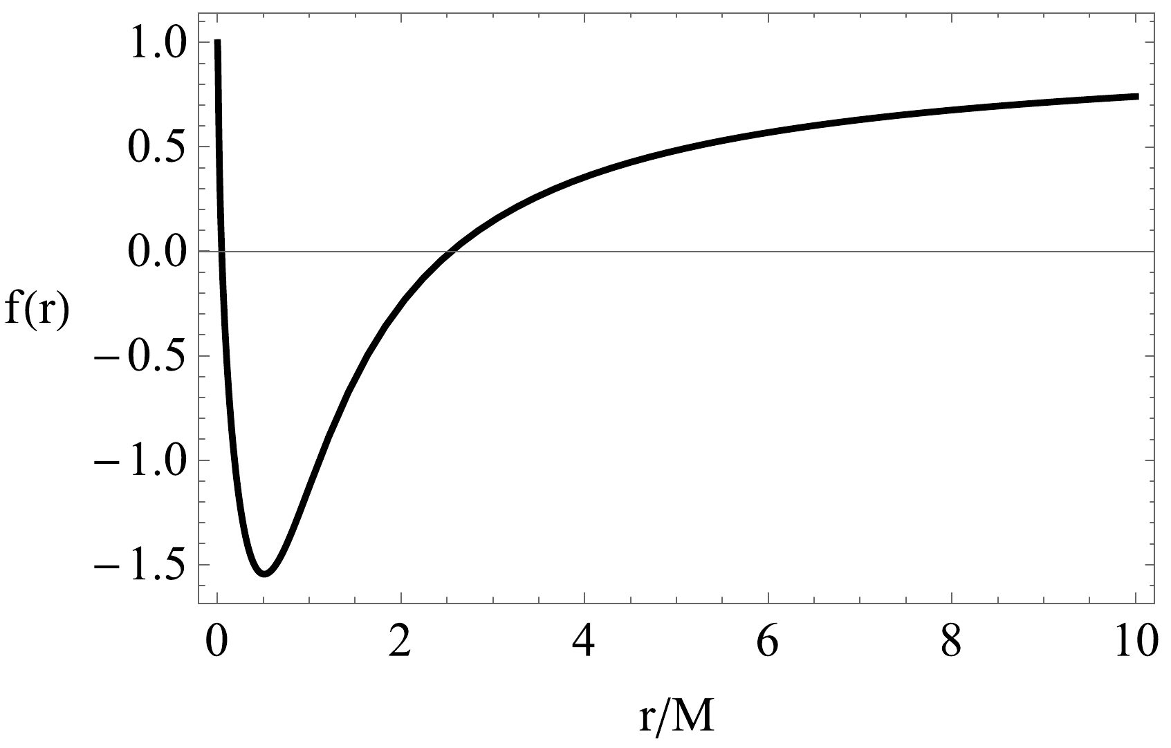
Figure 1. Metric function
$ f(r) $ as a function of r for specific choice of parameters.$ \begin{eqnarray} T=\frac{f'(r)}{4 \pi}\Big|_{r_+}. \end{eqnarray} $

(70) In Fig. 2 (left panel), the Hawking temperature is plotted for a specific domain of parameters. Note that the negative values of temperature are not of physical interest. Setting
$ f(r_+)=0 $ , we obtain$ M_{+} $ and$ T_+ $ . Then, by integrating the first law${\rm d} M=T{\rm d}S$ , the entropy for this black hole can be obtained as
Figure 2. (color online) Left panel: Hawking temperature T plotted as a function of horizon
$ r=r_+ $ . Right panel: Plots of the specific heat capacity for a particular choice of parameters.$ \begin{eqnarray} {\rm d}S=\frac{1}{T}\bigg(\frac{\partial M_+}{\partial r_+ }\bigg)_{Q,\alpha}{\rm d}r_+, \end{eqnarray} $

(71) and the heat capacity can be evaluated via
$ C=\frac{\partial M}{\partial T}\Big|_{r_+}=\frac{\partial M}{\partial r}\frac{\partial r}{\partial T}\Big|_{r_+}. $

(72) In general, we can evaluate these expressions numerically. Note here that if
$ C_+>0 $ , the black hole is said to be stable, and for$ C_+ <0 $ , we conclude that the black hole is unstable. Basically, C vanishes at some$r=r_{\rm ext}$ , which means that not all the values in the range shown in Fig. 2 are allowed for C. Moreover, there is a singularity and a sign change, which signals a phase transition at the maximum temperature. -
We used the modified expression for the gravitational and electric potentials inspired by the string T-duality to obtain an exact charged solution in the 4D EGB theory of gravity with a cosmological constant. We demonstrated that the solution also exists in the regularized 4D EGB theory. We identified a problem regarding the additional dynamical scalar field, which has to be infinitely strongly coupled to reproduce the results of the 4D EGB theory. Following the arguments in [22, 23], one can find a consistent theory and solve this issue by adding an appropriate counter term to the Hamiltonian [22, 23], which leads to the Lorentz violating theory by breaking a part of diffeomorphism invariance. We used the 3+1 decomposition to show the correspondence between the solution in the 4D EGB theory and that in the non-relativistic Horava–Lifshitz theory. The black hole solution reported here is regular and free from singularity. As a special case, we obtained well known solutions in the literature such as the regular AdS Bardeen black hole, AdS charged black hole in 4D EGB gravity, and AdS RN solution in general relativity. To this end, we investigated thermodynamical aspects such as the the Hawking radiation and specific heat capacity. We showed a close connection between the quantum gravitational Bardeen black hole solution and the GUP principle. In the near future, we will study phenomenological aspects of the solution reported in this study.
-
I would like to thank the referee for very helpful and constructive comments that helped me improve the paper significantly.
Charged AdS black holes with finite electrodynamics in 4D Einstein-Gauss-Bonnet gravity
- Received Date: 2022-11-05
- Available Online: 2023-03-15
Abstract: Using a modified expression for the electric potential in the context of T-duality [Gaete and Nicolini, Phys. Lett. B, 2022], we obtained an exact charged solution within the 4D Einstein-Gauss-Bonnet (4D EGB) theory of gravity in the presence of a cosmological constant. We show that the solution also exists in the regularized 4D EGB theory. Moreover, we point out a correspondence between the black hole solution in the 4D EGB theory and the solution in the non-relativistic Horava–Lifshitz theory. The black hole solution is regular and free from singularity. As a special case, we derive a class of well known solutions in the literature.


 DownLoad: