Shadow and gravitational weak lensing around a quantum-corrected black hole surrounded by a plasma

In general relativity (GR), astrophysical black holes (BHs) are formed in the collapse of a self-gravitating massive star's end-state evolution, making GR the most successful theory of gravity. It is worth noting, however, that there are theoretical challenges that need to be addressed, such as quantization, dark matter and energy issues, singularities inside BHs [1] and at the beginning of the universe [2, 3], where GR breaks down. Additionally, GR does not incorporate quantum principles, leaving the question of unifying GR and quantum mechanics unsolved [4, 5]. These challenges have been explored from various perspectives, with modified and quantum theories of gravity being considered as potential solutions. Testing modified theories of gravity in astrophysical scenarios is crucial in finding a final theory that can address the challenges of GR. Despite these challenges, recent observations such as gravitational waves (GWs) [6, 7] and the BH shadow [8, 9]) would provide promising insights into the issues of GR.

As previously stated, GR is unable to incorporate quantum principles and find a solution to cosmological Big Bang and black hole singularities. Therefore, quantum theories of gravity may offer a potential solution to address these singularities through quantum effects. In this regard, loop quantum gravity (LQG) has been considered a non-perturbative theory of quantum gravity [10]. Since then, its techniques have been extensively applied to finding solutions to avoid these singularities in loop quantum cosmology; see [11−17]. It is important to note that models describing black hole solutions in LQG have been developed in recent years. For example, a regular static black hole solution, known as the self-dual black hole, was obtained within a mini-superspace framework through the polymerization procedure in LQG [18], exhibiting self-duality associated with T-duality principles [19, 20]. There has been extensive analysis providing insights into the nature of quantum black hole solutions and focusing on examining the quantum effects within the LQG framework; see [21−29]. Additionally, it is worth noting that there has been an increase in activity in recent years, with the phenomenological study of loop quantum black holes being extensively explored in various contexts; see [30−37].

The detection of the first image of BH [8, 9] has opened up new avenues to develop theoretical models that can test various theories of gravity by exploring BH shadows. For a BH shadow, light can follow geodesics and make circles around the BH, leading to a dark disk. This analysis was first conducted for the Schwarzschild BH [38], together with its image [39]. It is envisioned that the BH shadow can be observed as a dark region surrounded by the light ring in the sky. This dark disk causes the formation of the BH shadow by trapping light that cannot escape from the gravitational pull. Studying BH accretion disks is crucial in gaining a deeper understanding of BH characteristics and the spacetime geometry. Later on, the BH shadow was explored by Amarilla et al for a rotating Kaluza-Klein dilaton BH [40] and was also extended to the Einstein-Maxwell-Dilaton-Axion BH [41]. Since then, there has been an increase in activity in recent years, where the BH shadow has been explored from various perspectives [42−51]. It is also worth noting that the BH shadow was studied for a rotating BH including a scalar dilaton field [52], a charged BH that involves a dilaton field within the Einstein-Maxwell-scalar theory [53], and regular BHs [54]. It was shown that the BH deformation parameters can have a significant effect on the BH shadow characteristics (see, e.g., [55]) and the recent EHT observations can be used to obtain restrictions on theoretical BH shadow models [56]. Additionally, it should be noted that the modified theory of gravity (MOG) was tested through the BH shadow analysis in both rotating and non-rotating cases [57−59].

In an astrophysical scenario, BHs can be surrounded by a plasma medium in their nearby environment, where the optical properties of BHs, such as the shadow and gravitational lensing effects, can be significantly altered due to the surrounding plasma effect. It is envisioned that gravitational lensing effects occur due to the highly deflected light traveling around a BH in the strong field regime. This led to the first theoretical experiment in which GR was successfully tested through gravitational lensing analysis (see, e.g., [60]). In this regard, gravitational lensing effects can also provide excellent tests for probing spacetime geometry, especially very close to the BH horizon. Therefore, in recent years, there has been increased research activity addressing gravitational lensing effects in the weak form [see, e.g., 61−72] in the presence of a plasma medium [see, e.g., 73−80] within various gravity scenarios.

BHs are, as depicted, the most fascinating and intriguing astrophysical objects. Therefore, they are currently under scrutiny from various theoretical and observational perspectives. This analysis provides valuable insights into BH properties within different models, such as a quantum-corrected BH solution, which incorporates quantum corrections within the Oppenheimer-Snyder model in the context of loop quantum gravity [81]. In this solution, the BH mass sets a lower bound due to quantum corrections, leading to a different background geometry compared to BH solutions in GR. This quantum-corrected BH solution was developed as a modification of the Schwarzschild BH, addressing the BH singularity. It is important to note that its geometry can differ from other BH solutions derived within loop quantum gravity, showing that the collapsing process depends on whether the collapsing matter density extends to the Planck scale. If this density is of the order of the Planck scale, the collapsing process transforms into a bounce expansion epoch. Following [81] there have been several investigations [82−86] addressing properties of this quantum-corrected BH spacetime in various situations. Therefore, it is also essential to investigate the optical properties of a quantum-corrected BH to understand potential deviations from GR resulting from quantum corrections in loop quantum gravity. In this paper, we explore the optical properties of a quantum-corrected BH, including the BH shadow and gravitational lensing effects in the presence of a plasma medium. This analysis enhances our understanding of the unique features of quantum-corrected BH geometry.

This paper is organized as follows: In Sec. II we briefly review a quantum-corrected BH spacetime and discuss the formalism used to further model the photon motion and the BH shadow in a plasma medium. In Sec. III, we study gravitational lensing effects by a quantum-corrected BH, together with plasma medium effects resulting from both uniform and non-uniform cases. Further, we analyze a magnification of gravitationally lensed image around a quantum-corrected BH in Sec. IV. Finally, we give our concluding remarks in Sec. V. We shall for simplicity use $ c = G = M = 1 $ throughout the paper.

Here, we will briefly review the dynamics of the photon motion to explore the BH shadow under the combined effects of plasma medium and the quantum corrections resulting from the loop quantum gravity. The corresponding metric describing a static and spherically symmetric quantum-corrected BH in Boyer–Lindquist coordinates $ (t, r, \theta, \phi) $ is given by [81]

with

where M refers to the Arnowitt–Deser–Misner mass, while $ \alpha = 16\sqrt{3}\pi\gamma^3\ell_p^2 $ to the quantum corrected parameter, together with the Immirzi parameter γ and the Planck length $ \ell_p = \sqrt{G\hbar} $. For further analysis we shall for simplicity consider α as a dimensionless quantity by considering $ \alpha\to \alpha/M^2 $ and setting $ G = c = 1 $. here, it is worth noting that the metric describing the quantum-corrected BH through Eq. (1) can be reduced to the Schwarzschild BH in the limit of $ \alpha\to 0 $.

Photon motion around the quantum-corrected BH immersed in the plasma medium: Here, we consider the formalism used to model and study the motion of the photon around the quantum-corrected BH on the basis of the Hamilton-Jacobi equation. To this end, we first write the Hamiltonian for null geodesics around the BH in the presence of the plasma medium, which is given by [87]

where $ x^{\alpha} $ refers to the spacetime coordinates, $ u^\beta $ and $ p_\alpha $ are the four-velocity and momentum of the photon, respectively. In addition, n is the refractive index, i.e., $ n = \omega/k $, k is the wave number. We can write the following equation for the refractive index [88]

where $ \omega^2_{p}(x^\alpha) = 4 \pi e^2 N(x^\alpha)/m_e $ is the plasma frequency, with $ m_e $ and e refer to the electron mass and charge, and N is the number density of the electrons. Using the expression $ \omega^2 = ( p_\beta u^\beta )^2 $, we can find the photon frequency as

If r tends to infinity ($ r \rightarrow \infty $), the lapse function $ f(r) $ tends to 1. Hence, $ \omega(\infty) = \omega_0 = -p_t $ which expresses the photon energy at spatial infinity [89]. $ \omega_0 $ can be restricted using the photon geodesics $ {\cal H} = 0 $ as

From the physical point of view, the meaning of this restriction is that photon frequency at a given point ($ \omega(r) $) must be greater than the plasma frequency at the same point. This rule can be consistently applied to light propagation in a plasma. Hence, the BH shadow can have different forms from the vacuum case $ \omega_p = 0 $. Using the Eq. (4), we can rewrite the Eq. (3) for the light geodesics in the presence of a plasma medium in the following form

The four velocities for the photon can be written in the equatorial plane ($ \theta = \pi/2 $) as

where $ \dot x^\alpha = \partial {\cal{H}}/\partial p_\alpha $. The orbit equation is obtained using Eqs. (9) and (10) as follows:

The above equation can be written for the photon geodesics $ {\cal{H}} = 0 $

where the following relation holds well

A light ray comes from infinity, reaches a minimum at a radius $ r_{ps} $, and then returns to infinity. Mathematically, it corresponds to a turning point of the $ \gamma^2(r) $ function. Hence, the radius of the photon sphere can be determined from the following equation

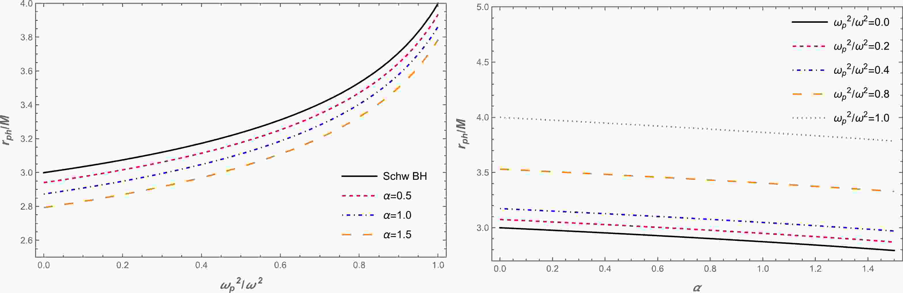
It is hard to solve the above equation; therefore, we use the numerical method and plot the dependence of the photon radius on the BH and plasma parameters in Fig. 1. It is evident from Fig. 1 that the value of the photon radius increases with the increase of the plasma parameter. Moreover, there is a decrease in the photon radius with an increase in the quantum corrected parameter α. This corresponds to the interpretation of the quantum-corrected parameter as a repulsive gravitational charge, which physically manifests in a change of the causal structure, weakening the strength of the gravitational field at a close distance near the quantum-corrected BH. This allows for photon orbits to remain closer to the BH.

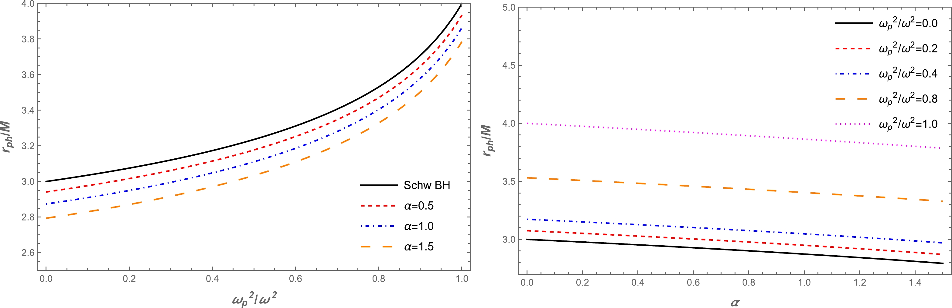
Figure 1.  (color online) Left panel: The radius of the photon sphere as a function of the plasma frequency for different values of the α parameter. Right panel: The dependence of the radius of the photon sphere on the α parameter for different values of the plasma frequency.

The quantum-corrected black hole shadow in the plasma medium: Now, we move to study the BH shadow radius in the presence of the plasma medium. We demonstrate the photon's trajectory in Fig 2 to provide more information. It can be shown from Fig 2 that if the angle α approaches $ \alpha_{sh} $, the radius of the shadow R tends to $ r_{ps} $. Then, we can explore the BH shadow using this figure. We can define the angular radius $ \alpha_{sh} $ of the BH as follows [42, 8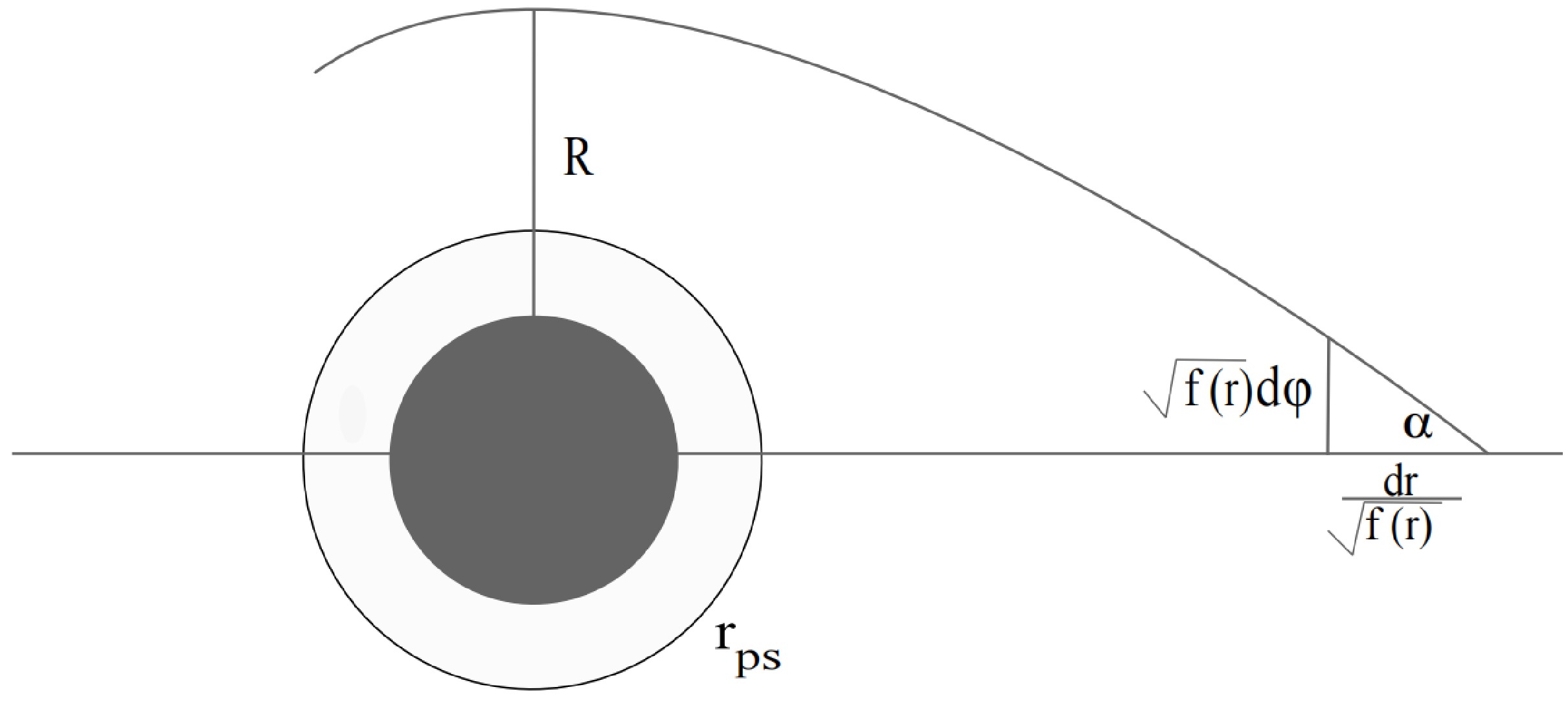9]

Figure 2.  The schematic diagram of the light bending around BH. As R approaches $ r_{ps} $, the angle α converges to the angular radius of the BH shadow $ \alpha_{sh} $.

where $ r_{\text{ps}} $ and $ r_{\text{o}} $ refer to the locations of the photon sphere and observer, respectively. We can approximate the radius of the BH shadow for the observer located at a sufficiently large distance from the BH as [89]

We demonstrate the dependence of the BH shadow on the plasma and BH parameter in Fig. 3. We can see from this figure that the radius of the BH shadow decreased with the increase of the plasma parameter. In addition, under the influence of the α parameter the radius of the BH shadow decreased slightly. Now we assume that the compact objects Sgr A* and M87* are static and spherically symmetric, even though the observation obtained by the EHT collaboration does not support the assumption made here. Then, we try to theoretically explore the lower limits of the α parameter, using the data provided by the EHT collaboration project. We chose the α parameter and plasma frequency for constraint. We can constraint these two quantities α and $ \omega^2_p/\omega^2 $ using the observational data provided by the EHT collaboration regarding the shadows of the supermassive BHs Sgr A* and M87*. The angular diameter $ \theta_{M87*} $ of the BH shadow, the distance from Earth and the mass of the BH at the center of the M87* are $ \theta_{M87*} = 42 \pm 3 \mu as $, $ D = 16.8 \pm 0.8 M pc $ and $ M_{M87*} = 6.5 \pm 0.7 \times 10^9 M_{\odot} $ [8], respectively. For Sgr A*, the data provided by the EHT collaboration are $ \theta_{Sgr A*} = 48.7 \pm 7 \mu $ $ D = 8277 \pm 9 \pm 33 pc $ and $ M_{Sgr A*} = 4.297 \pm 0.013 \times 10^6 M_{\odot} $ (VLTI) [90]. Using this information, one can calculate the diameter of the shadow caused by the compact object per unit mass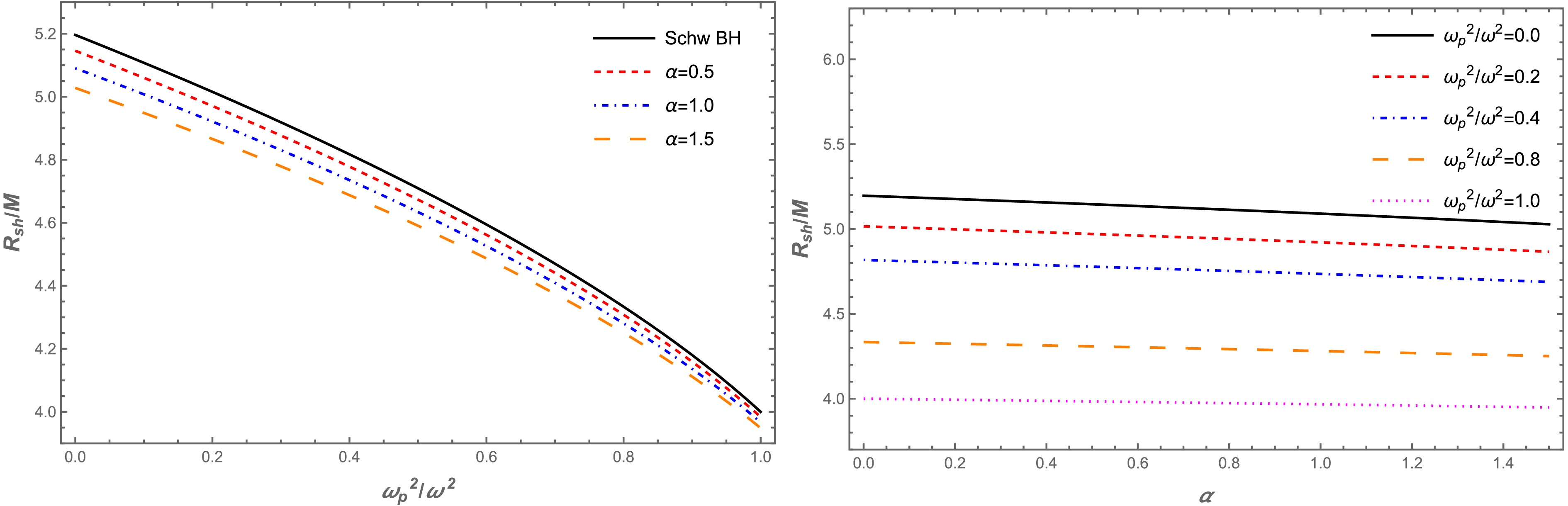 as [91]

Figure 3.  (color online) Left panel: The radius of the BH shadow as a function of the plasma frequency for different values of the α parameter. Right panel: The dependence of the radius of the BH shadow on the α parameter for different values of the plasma frequency.

Using the expression $ d_{sh} = 2R_{sh} $ one can easily obtain the expression for the diameter of the BH shadow. Note that the distance D is considered a dimension of M [8, 9]. The diameter of the BH shadow $ d^{M87*}_{sh} = (11 \pm 1.5)M $ for M87* and $ d^{Sgr*}_{sh} = (9.5 \pm 1.4)M $ for Sgr A*. The lower limits on the quantities α and $ \omega^2_{p}/\omega^2 $ for the supermassive BHs at the centers of the galaxies Sgr A* and M87* can be found using the observational EHT data. It is shown in Fig. 4.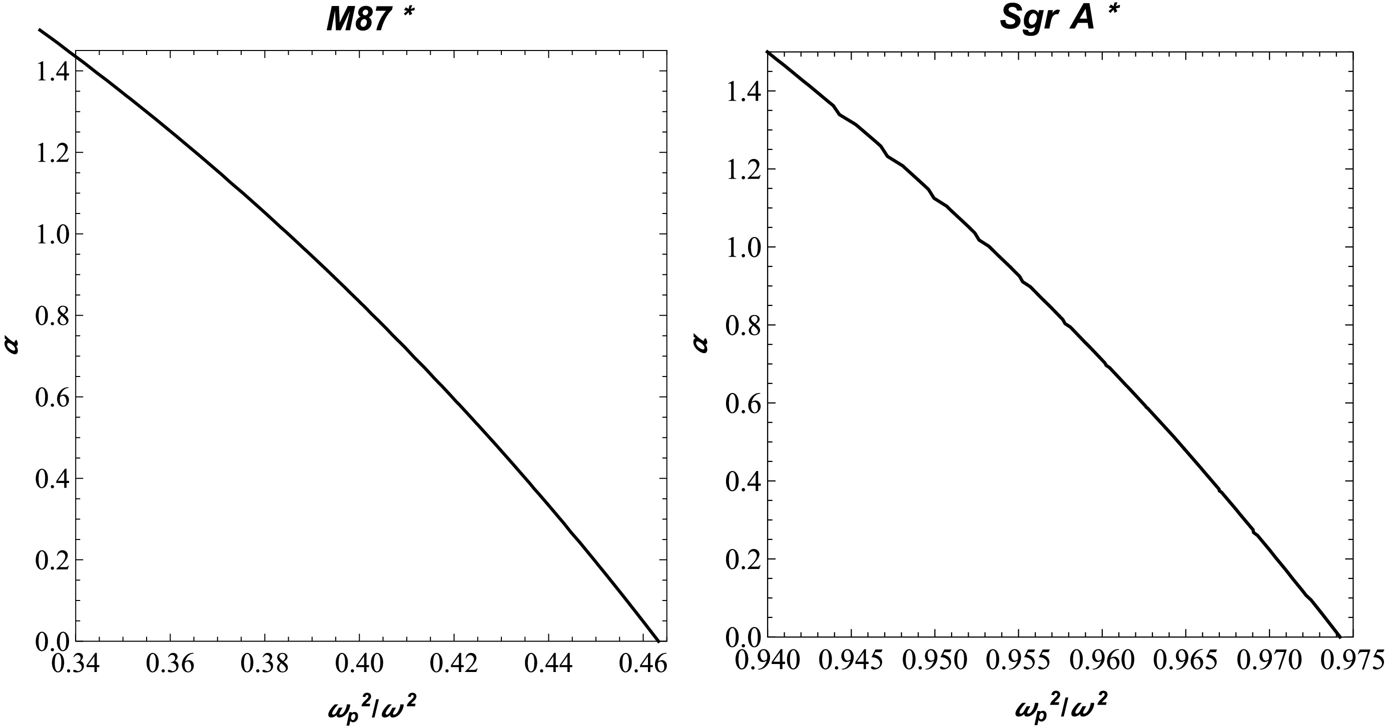

Figure 4.  The constrained values of the α parameter and $ \omega^2_{p}/\omega^2_0 $ for supermassive BHs sitting at the center M87 and Sgr $ A^{\star} $ galaxies.

In this section, we explore the weak gravitational lensing for two different plasma distributions, i.e., uniform and non-uniform plasma. For that, we first represent the weak-field approximation as [64, 92]

where $ \eta_{\alpha \beta} $ and $ h_{\alpha \beta} $ refer to the expressions for Minkowski spacetime and the perturbation gravity field, respectively. One can write the following conditions for them

One can write the following equation for the deflection angle around the quantum-corrected BH as [92]

where ω and $ \omega_{p} $ are the photon and plasma frequancies, respectively. Further, we expand the metric functions into a Taylor series for calculations. The line element can be written as

with $ ds^2_0 = -dt^2+dr^2+r^2(d\theta^2+\sin^2\theta d\phi^2) $. After that, we can define the components of $ h_{\alpha \beta} $ as the perturbations which are written as follows:

with $ \cos^2\chi = z^2/(b^2+z^2) $ and $ r^2 = b^2+z^2 $. One can write the first derivatives of $ h_{00} $ and $ h_{33} $ with respect to the radial coordinate as follows

We can write the deflection angle in the following form

with

In the following, we explore the impact of plasma density distributions on the deflection angle from two different perspectives: uniform and non-uniform plasma cases.

Uniform plasma distribution: In this part, we consider a uniform plasma surrounding the quantum-corrected BH and examine its impact on the gravitational angle of deflection. Therefore, we rewrite Eq. (27) for uniform plasma

One can define the deflection angle influenced by a uniform plasma using Eqs. (24), (27) and (28). The dependence of the deflection angle on the impact parameter b is demonstrated in Fig. 5. The left panel corresponds to the vacuum case. There is a slight decrease with the increase of the α parameter. The right panel corresponds to the uniform plasma case. Comparing the two panels, we can say that the deflection angle increases in the uniform plasma than in the vacuum case. In Fig. 6, we demonstrate the role of plasma parameters on the deflection angle. Note that the values of the deflection angle increase under the influence of the uniform plasma frequency.

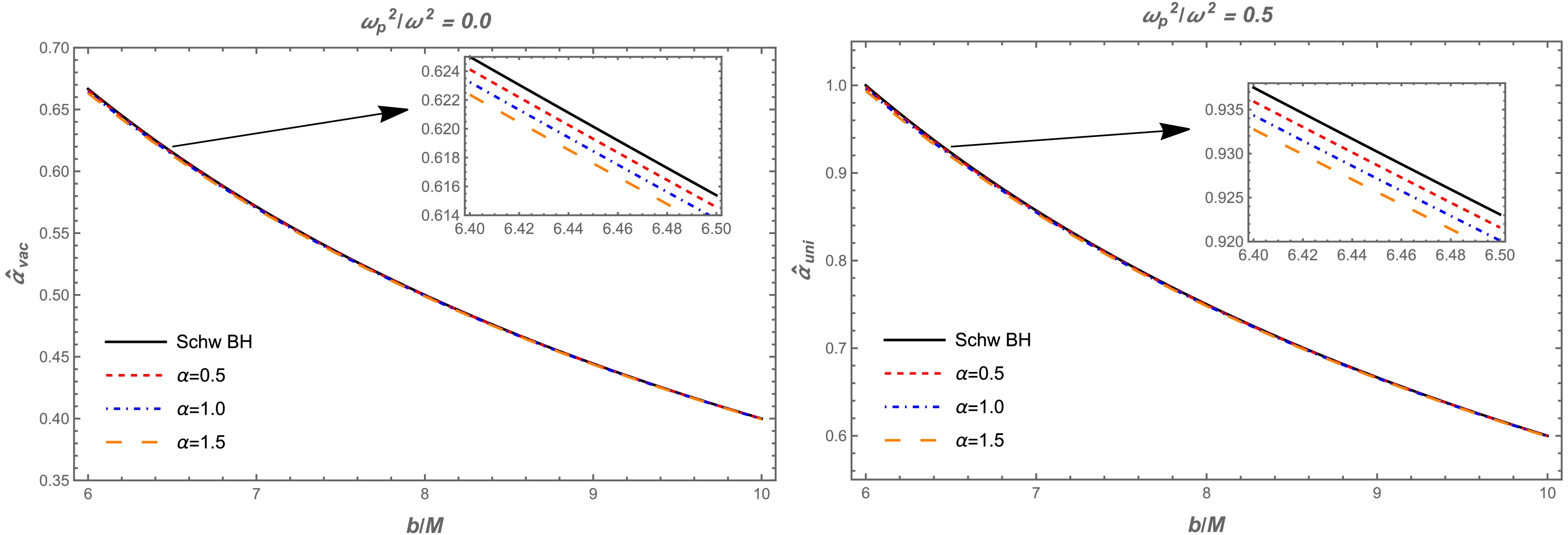
Figure 5.  (color online) Left panel: The dependence of the deflection angle $ \hat{\alpha}_{vac} $ on the impact parameter b for the different values of the α parameter; here, $ \omega^2_p / \omega^2 = 0 $. The dependence of the deflection angle $ \hat{\alpha}_{\text{uni}} $ on the impact parameter b for the different values of the parameter α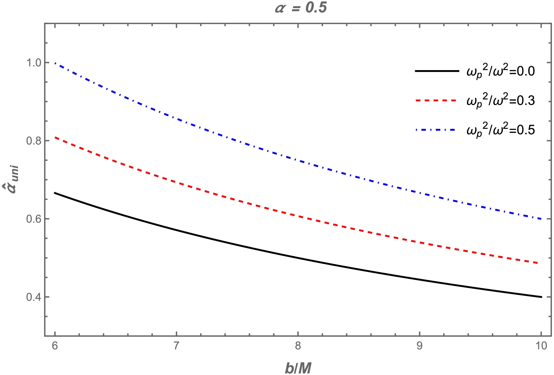 (right panel).

Figure 6.  (color online) The deflection angle $ \hat{\alpha}_{\text{uni}}$ as a function of the impact parameter b for different values of the plasma frequency. Here we have set $ \alpha=0.5$.

Non-uniform plasma distribution: Thereafter, we consider the non-singular isothermal sphere (SIS). SIS density distribution can be defined as [92]

where $ \sigma^2_{\nu} $ refers to an one-dimensional velocity dispersion. With this in mind, the analytical expression for the plasma concentration is given as

where $ m_p $ and k refer to proton mass and a dimensionless constant, respectively. Then one can find the plasma frequency in the following form

To conduct a more detailed analysis of the non-uniform plasma (SIS) effect, it is necessary to derive the explicit expression for the deflection angle around BH. It can be written as

By u Eqs. (24), (28), and (33), we can derive the expression for the deflection angle and introduce the additional plasma constant $ \omega^2_c $ in its explicit form. [92]

where $ R_S = 2M $. In Fig. 7, we have demonstrated the dependence of the deflection angle around the quantum-corrected BH on the impact parameter b for different values of the α parameter and the non-uniform plasma frequency. We can observe from Fig. 7 that the deflection angle decreases with the increase of the non-uniform plasma frequency. Moreover, there is a slight decrease in the values of the deflection angle with an increase of the α parameter. Note that the non-uniform plasma has an opposite effect on the deflection angle compared with the uniform plasma case. To be more informative we have plotted both cases in a single plot by making the values of the plasma frequencies the same (see Fig. 8).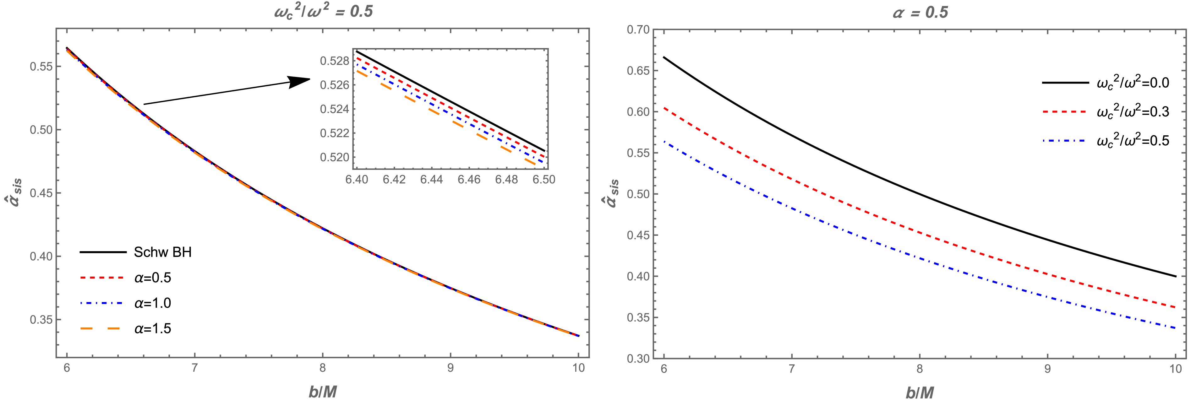

Figure 7.  (color online) The dependence of the deflection angle $ \hat{\alpha}_{\text{sis}} $ on the impact parameter b for the different values of the parameter α (left panel) and the plasma frequency (right panel).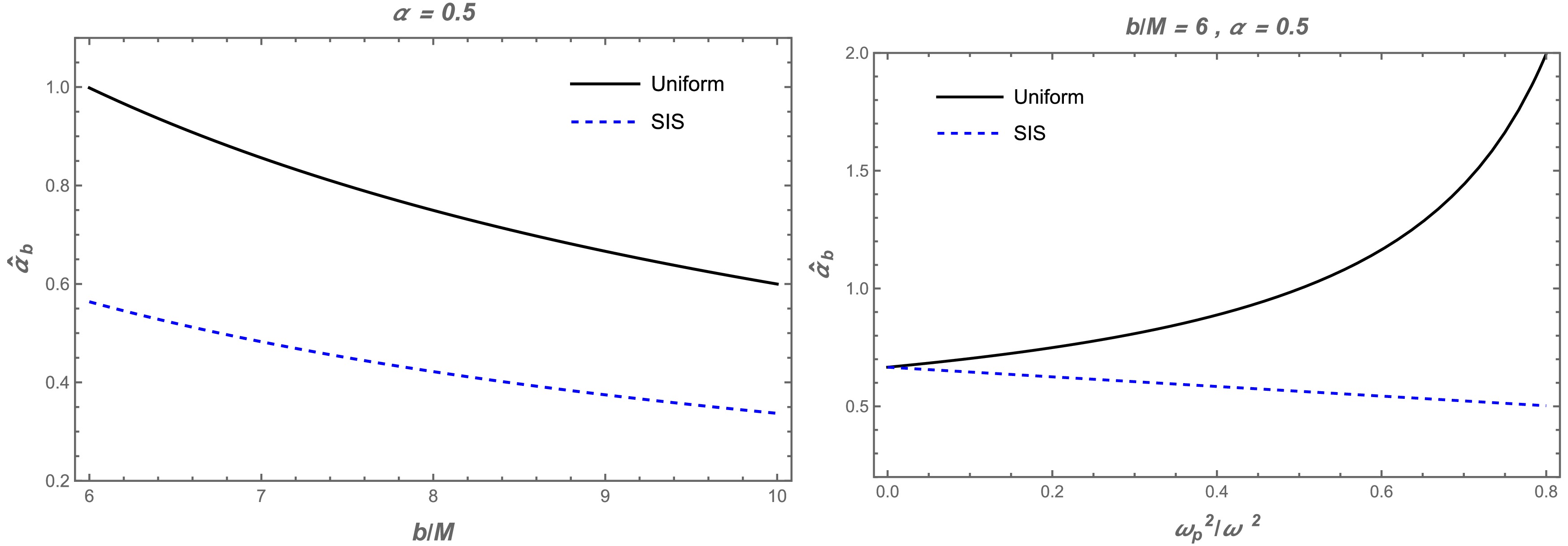

Figure 8.  (color online) Left panel: The dependence of the deflection angle $ \hat{\alpha }_{\text{b}} $ on the impact parameter b. Here, α parameter equals to $ 0.5 $. Right panel: the deflection angle $ \hat{\alpha }_{\text{b}} $ against the plasma parameters. The other parameters are $ b/M = 6 $ and $ \alpha = 0.5 $.

In this section, we study the magnification of the gravitationally lensed image around the quantum-corrected BH using the deflection angle of the light. With this in mind, we present the following equation, which combines the light angles $ \hat{\alpha_b} $, θ, and β around the black hole [64, 93]

where $ D_\mathrm{d} $ is the distance between the lens and the observer, $ D_\mathrm{s} $ the source and the observer, $ D_\mathrm{d} $ the lens and the observer, $ D_\mathrm{ds} $ the source and the lens. Also, θ and β refer to the image's angular position and β the source's angular position, respectively. One can write the angular position of the source β using Eq. (35) as

with $ \xi(\theta) = |\hat{\alpha}_b|\,b $ and $ b = D_\mathrm{d}\theta $. It is important to note that the shape of the image can be identified as Einstein's ring with a radius of $ R_s = D_\mathrm{d}, \theta_E $, assuming it appears as a ring. In this case, the corresponding angular part $ \theta_E $ is defined by

Then the magnification of brightness yields

where $ I_* $ and $ I_\mathrm{tot} $ refer to the unlensed brightness of the source and the total brightness, respectively. After that one can write the magnification of the source as follows [94−96]

The magnification of the source is then expressed as, where $ x = {\beta}/{\theta_E} $ is a dimensionless parameter, and $ \mu_{+}^{\mathrm{pl}} $ and $ \mu_{-}^{\mathrm{pl}} $ represent the images. As a result, the total magnification can be written a linear combination of the images as follows:

In the next, we explore the magnification of the source for two different cases: uniform and non-uniform plasma distributions surrounding the quantum-corrected BH.

Uniform plasma medium case: In this part, we consider the uniform plasma medium to explore the magnification of the lensed image as mentioned above. Therefore, one can rewrite the Eq. (41) for uniform plasma that surrounds the quantum-corrected BH in the following form

Here, the images $ (\mu^{pl}_+)_{uni} $ and $ (\mu^{pl}_-)_{uni} $ are defined by

and

with

We numerically investigated the total magnification in a uniform plasma case. Fig. 9 shows the dependence of the total magnification of the image $ \mu^\mathrm{pl}_\mathrm{tot} $ on the uniform plasma frequency for different values of the α parameter with a fixed value of the impact parameter $ b = 6M $. One can see from this figure that there is a slight decrease with the increase of the α parameter. Moreover, the values of the total magnification increase with an increase of the uniform plasma frequency.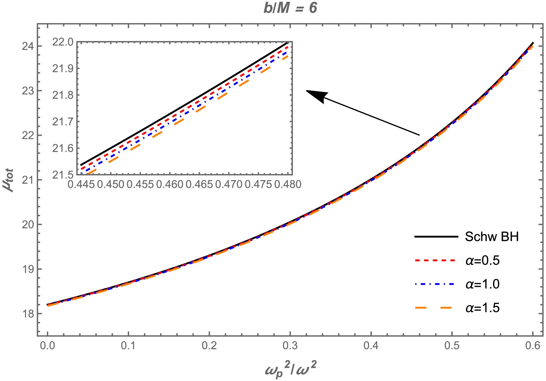

Figure 9.  (color online) The total magnification $\mu_{tot}$ as a function of the plasma frequency $\omega^2_{p}/\omega^2$ for different values of the α parameter. Here, $b=6M$.

Non-uniform plasma medium case: Afterwards, we study the behavior of the total magnification by considering the non-uniform plasma (SIS). We can write the following equations for the non-uniform plasma case

with

where $ x_{SIS} $ is

Using Eq. (46), the total magnification can be determined as a function of the plasma parameter. It can be seen from Fig. 10 that the total magnification decreases with the increase of the non-uniform plasma parameter. Moreover, one can deduce that the total magnification of lensed images decreases under the influence of the quantum corrected parameter α acting as a repulsive gravitational charge, which physically results in the weakening of gravitational field around the BH. The effect of α is the same for both uniform and non-uniform plasma distributions. However, we find that the total magnification decreases in the presence of non-uniform plasma compared to that of uniform plasma.

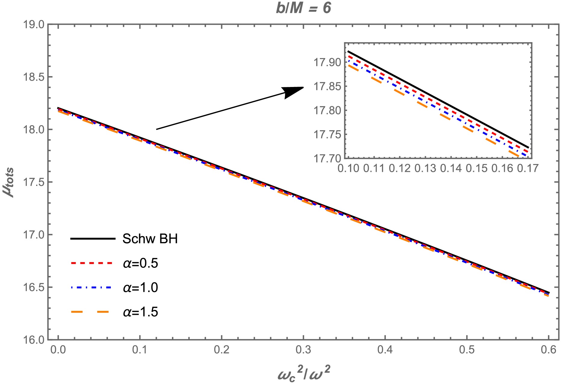
Figure 10.  (color online) The dependence of the total magnification $\mu_{tots}$ on the plasma frequency $\omega^2_{c}/\omega^2$ for different values of the α parameter. Here, $b=6M$.

In this paper, we considered a quantum-corrected BH in the Quantum Oppenheimer-Snyder model within the context of loop quantum gravity and investigated its optical properties, revealing intriguing deviations from GR. We first explored the motion of photons around a quantum corrected BH surrounded by a plasma medium. We derived numerical results showing the relationship between the radius of the photon sphere and the plasma frequency; see Fig. 1. We showed that the photon sphere radius grows with an increasing the plasma parameter, but it decreases with an increase in the quantum correction parameter α. We further studied the BH shadow under the combined effects of the quantum correction parameter and plasma medium parameter. Similarly, compared to photon radii, we also utilized a similar numerical method to determine the BH radius and showed that the BH shadow radius decreases under the combined effects of the plasma and quantum correction parameter, as seen in Fig. 3.

Additionally, we used the obtained results to determine the constraints on the quantum correction parameter, as the shadow size depends on the BH parameters, as shown in Fig. 4. Using observational data from M87$ ^{\star} $ and Sgr A$ ^{\star} $, we determined the possible range of constraints on the quantum correction and plasma parameters. Our findings on the constrained values can be helpful and potentially applied to M87$ ^{\star} $ and Sgr A$ ^{\star} $ images to provide insights and a constraint range on the quantum correction parameter within astrophysical observations, including observational data on gravitational lensing effects (see, e.g., [97−99]).

We further investigated the gravitational lensing in the weak form around a quantum-corrected BH, together with the effects of the plasma medium. For that, we considered two independent possible cases: uniform and non-uniform plasma cases. We then examined the behavior of the deflection angle resulting from the combined effects of the quantum correction and both uniform and non-uniform plasma parameters. We showed that the deflection angle $ \hat{\alpha}_{\text{uni}} $ decreases due to the quantum correction parameter α, while it increases with the rise in the uniform plasma parameter, as shown in Figs. 5 and 6. It does however decreases as a function of the impact parameter under the combined effects of quantum correction and uniform plasma parameters. When considering the non-uniform plasma, the deflection angle $ \hat{\alpha}_{\text{sis}} $ changes at a similar rate due to the combined effects of the quantum correction and non-uniform plasma parameters, resulting in the deflection angle shifting downward and decreasing to possibly smaller values; see Fig. 7. It is important to note that the light traveling through the uniform plasma medium can be strongly deflected compared to the non-uniform plasma, leading to a significant difference in the deflection angle for uniform and non-uniform plasma distributions (see, e.g., Fig. 8).

Finally, we explored a changing rate of the total magnification, $ \mu^{pl}_{tot} $, of the lensed image under the effect of the quantum correction parameter α, together with the effects of both uniform and non-uniform plasma distributions, as shown in Figs. 9 and 10. It was found that the curves of the total magnification shift downward to possibly smaller values as a consequence of the impact of the quantum correction parameter α, similarly to what is observed in the behavior of the deflection angle, while it increases/decreases significantly by the uniform/non-uniform plasma effects.

The results showed that the quantum correction parameter, α, can alter the null geodesics, resulting in the radii of the photon sphere and BH shadow decreasing under its effect. This behavior is consistent with the physical interpretation of the quantum correction parameter acting as a repulsive gravitational charge, which results in the weakening of the strength of the gravitational field at a close distance near the quantum-corrected BH. Additionally, this would be of primary astrophysical significance, as it does not exclude the effect of the quantum correction parameter, although small, together with the effects of the plasma medium. Our findings can help provide insights into the quantum-corrected BHs and can help explain and constrain the validity of alternative models to BHs in both GR and loop quantum gravity when making astrophysical observations and predictions.