Holographic image features of an AdS black hole in Einstein-power-Yang-Mills gravity

General Relativity (GR) is widely acknowledged as the preeminent theory of gravitation owing to its extensive validation through many observational studies and experiments [1]. The predictions of GR on black holes, immensely compact celestial objects in our universe, have attracted significant interest from physicists. Recently, the Event Horizon Telescope (EHT) Collaboration has revealed unprecedented images of the black hole located at the core of a radio galaxy, M87^* [2–7], and at the Milky Way's center, Sagittarius A^* (Sgr A^*) [8–13], providing compelling evidence for the existence of black holes. One of the most remarkable characteristics exhibited by these images is the presence of a dark region within a luminous ring structure. According to GR, the gravitational field in the vicinity of a supermassive black hole is so intense that it causes a significant curvature of spacetime. Consequently, the photons attempting to escape this region are ultimately captured by the black hole. Hence, from the observer's perspective, a dark area will be observed, which is called the black hole shadow [14–17]. Moreover, because of the powerful gravitational force around a black hole, a mass of matter will be accreted to form what is called an accretion disk. During the accretion process, part of the gravitational potential energy is converted into thermal radiation. Therefore, the accretion disk is generally considered a bright light source near the black hole. A portion of the light emitted from the accretion disk reaches the observer, resulting in the perception of a luminous structure, commonly referred to as the photon ring. Based on the findings reported by the EHT, the angular size of the photon ring surrounding Sgr A^* aligns closely with the shadow critical curve radius predicted by GR, with a deviation of no more than 10% [8–13]. The enhancement of EHT resolution and the emergence of experimental advancements such as the image of the black hole at the center of the Milky Way will inevitably impose higher demands on the theoretical study of black hole imaging. In the theoretical investigation of black hole imagery, photon rings and black hole shadows have attracted considerable interest. This is because their study not only elucidates the fundamental properties of black holes but also serves as a robust tool for constraining various gravitational models [18–38].

Despite extensive research on the properties of black hole shadows and their associated dynamics, which has provided significant insights into black hole physics, many mysteries remain to be unraveled using more realistic models. Studies have established that the ($ D + 1 $)-dimensional gravity theory in Anti-de Sitter (AdS) spacetime can be associated with the D-dimensional conformal field theory (CFT) owing to the AdS/CFT correspondence, which is also known as holography theory [39–41]. In a pioneering endeavor, Hashimoto et al. constructed holographic images of the Schwarzschild AdS black hole in the bulk using a given response function of quantum field theory (QFT) on the boundary within the framework of AdS/CFT duality [42, 43]. The results indicated the presence of a distinct circular structure in two-dimensional spherical thermal holographic images, namely, the Einstein ring, and the size of the ring is consistent with the size of the black hole photon ring observed using geometric optics. Considering that real quantum materials are typically engineered with a finite chemical potential [44], Liu et al. investigated the holographic image of a charged AdS black hole, where the complex scalar field serves as a probing wave in the bulk spacetime. They observed that the radius of ring remained unaffected by changes in the chemical potential, whereas it exhibited a distinct dependence on the temperature of the boundary system. Subsequently, the study of a black hole that is dual to a superconductor was conducted in [45], where the electric current of the superconductor under localized time-periodic external electromagnetic field was considered. They also acquired images that depicted the discontinuous changes in the size of the photon ring. Moreover, the investigation into holographic imaging of black holes has been expanded to encompass various gravitational frameworks [46–57]. In these studies, the characteristics of Einstein ring structures across various parameter spaces have been investigated. They have revealed that, for a given set of wave sources and optical systems, holographic images serve as an effective tool for differentiating between distinct types of black holes.

Recently, interest has increased in gravitational theories that incorporate non-linearity in the Maxwell fields. The discovery of the nonsingular nature of black hole solutions in nonlinear electrodynamics creates a new perspective on the physics of black holes [58]. Among them, the class of black hole solutions in power Maxwell invariant theory has been derived, where the Lagrangian density is given by $ ({F}_{\mu\nu} {F}^{\mu\nu})^q $, and q represents an arbitrary rational number [59]. Considering the Yang-Mills (YM) fields as an exception to the black hole no-hair theorem in both GR [60] and conformal gravity [61, 62], more investigations have been conducted on nonlinear models involving the coupling of nonabelian YM fields with gravity in the realm of GR [63]. As mentioned in [63], a black hole solution sourced by the power of YM invariant exists, i.e., $ ({F}^{(a)}_{\mu\nu} {F}^{(a)}{\mu\nu})^q $, where $ {F}^{(a)}_{\mu\nu} $ represents the YM field with its internal index $ 1\leq a \leq \frac{(D-1)(D-2)}{2} $. Such solutions successfully recover the D-dimensional Einstein-Yang-Mills (EYM) black holes in AdS spacetime if the power exponent is taken as $ q=1 $ [64, 65]. The study of black hole properties within the framework of Einstein-power-Yang-Mills (EPYM) gravity has revealed novel and intriguing phenomena, including van der Waals phase transitions and critical behavior [66, 67], Joule-Thomson expansion [68, 69], and the quasinormal mode and optical properties of the black hole [70].

Motivated by the aforementioned research, we aimed to construct holographic images of a black hole within the framework of EPYM gravity. Fundamentally, the photon ring exhibits variations depending on the specific bulk dual geometry, thereby inducing alterations of corresponding holographic response. Therefore, we are prompted to investigate the behavior of the lensed response of the black hole in EPYM gravity and construct holographic images to study the potential impacts of the relevant physical quantities on the resulting holographic images. As an essential reference, the alteration of the power exponent q will evidently impact the geometric structure of spacetime. Our concern lies in whether this alteration will be applied to the holographic image and how it will change the features of images. Moreover, in the background of EPYM gravity, the chemical potential of the boundary system is modified. We extensively investigate whether the chemical potential has distinct implications for holographic images when compared with those resulting from the charged black hole in [44]. This could potentially serve as an effective means of differentiating these two gravitational models.

The remainder of this paper is outlined as follows. In Sec. II, we present a holographic construction of the Einstein ring for an AdS black hole, where the scalar field serves as a probing wave in the bulk spacetime. In Sec. III, we provide a holographic setup of an AdS black hole under EPYM gravity and extract its corresponding lensed response function for analysis. In Sec. IV, we investigate the formation of Einstein rings within our theoretical analysis using an optical system composed of a convex lens and spherical screen. Furthermore, we not only present the brightness curve of the resulting ring but also conduct a comparative analysis with the ring obtained through optical approximation. The final section presents the conclusion.

Owing to the phenomenon of gravitational lensing, the light emitted from a distant galaxy can undergo distortion and manifest as an arc or multiple separate images when it passes through an intermediate galaxy along the line of sight. When two galaxies are perfectly aligned, the distorted light forms a ring-shaped structure that surrounds the foreground galaxy, commonly known as an Einstein ring. The Einstein ring serves as one of the most compelling manifestations of GR in the cosmos, providing a unique opportunity to investigate colossal galaxies. If the intermediate galaxy were to be substituted with a black hole, the resulting observed image would inherently yield an abundance of valuable insights regarding the characteristics and properties of the black hole. From this perspective, Hashimoto et al. [42, 43] constructed a holographic Einstein ring of the black hole in Schwarzchild-AdS₄ spacetime (Sch-AdS₄) based on the AdS/CFT correspondence. In Refs. [42, 43], the QFT is considered on $ R_t \times S^2 $, and an external source is introduced on $ S^2 $, where the external source is mapped to the boundary condition of the bulk field. The probe wave is emitted from the source located on the AdS boundary, diffracted by the black hole as it traverses through the spacetime of the black hole, and ultimately reaches another point on the AdS boundary, resulting in a lensed response. The asymptotic data of the bulk field corresponds to the response function in relation to an external source. Based on this response function, holographic images of an AdS black hole can be constructed. Consequently, they discovered a correspondence between the resultant Einstein ring and the size of the black hole photon ring determined through geometric optics calculations.

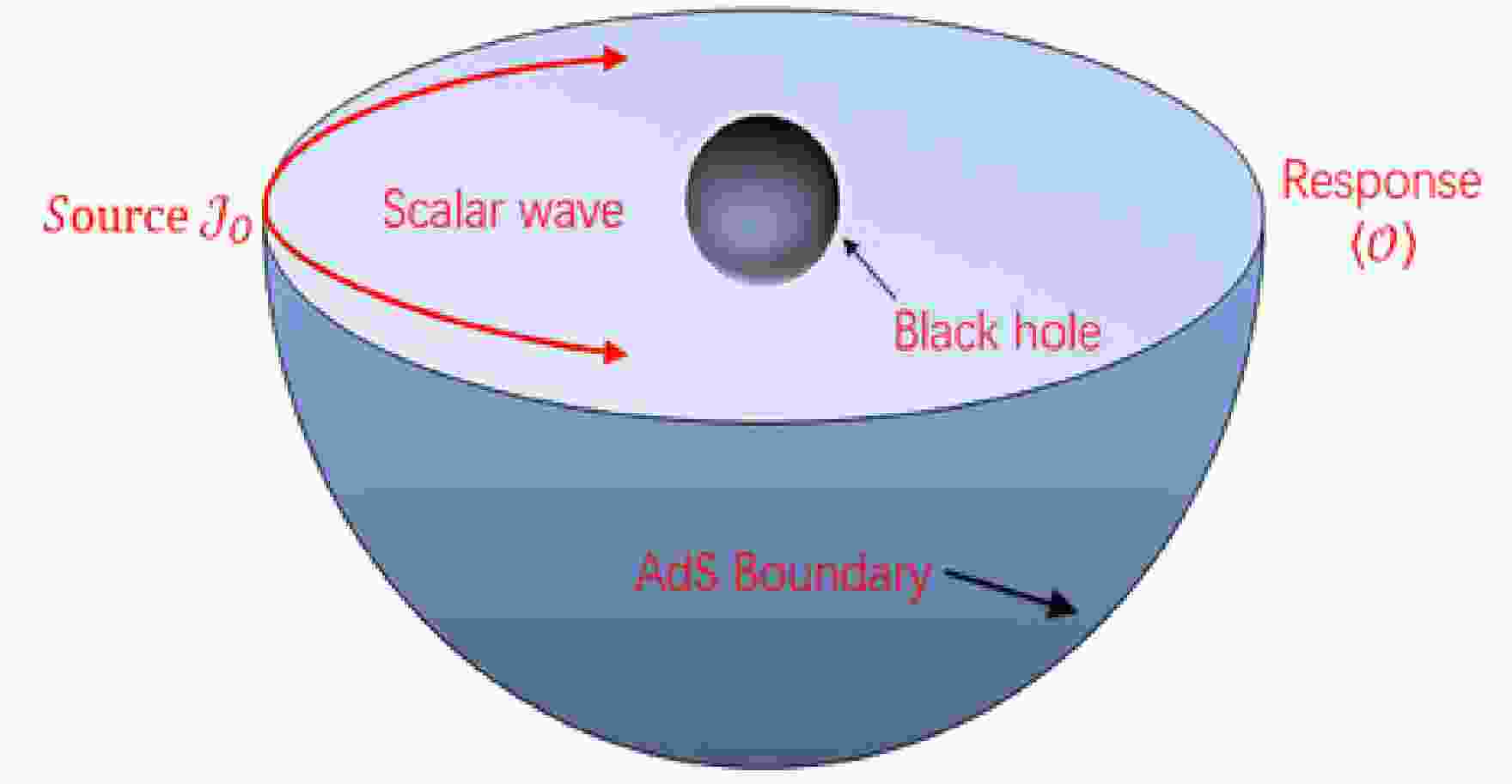
In this study, we apply this concept to the (2+1)-dimensional boundary CFT on a 2-sphere $ S^2 $ at the finite temperature and chemical potential. We consider placing a time-periodic localized Gaussian source with frequency $ \hat{\omega} $ on one side of the AdS boundary, as shown in Fig. 1. The (2+1)-dimensional boundary CFT on the 2-sphere $ S^2 $ is dual to a black hole in the global AdS₄ spacetime or a massless bulk scaler field in this spacetime. Motivated by the boundary conditions imposed by the time period, the scalar wave generated by the source can be injected into the bulk from the AdS boundary and propagated within the spacetime of a black hole in the bulk. The selected Gaussian source, when selected as an axially symmetric monochromatic oscillating Gaussian source and localized at the south pole of the AdS boundary $ \theta = \pi $, can be expressed as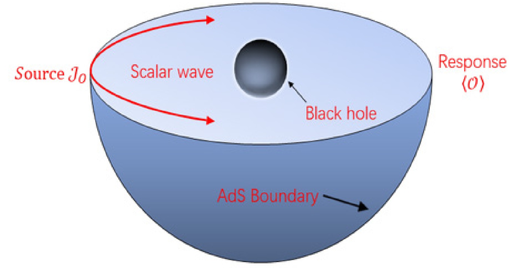

Figure 1.  (color online) Monochromatic Gaussian source located at a point on the AdS boundary, and its response is observed at another point on the same boundary.

where

Here, $ \chi_e $ and θ represent coordinates, and σ is the width of the scalar wave. For $ \sigma \ll 1 $, the negligible value of the Gaussian tail enables the decomposition of the Gaussian function into scalar spherical harmonics, that is

The corresponding coefficients $ C_{\zeta0} $ of the spherical harmonics $ Y_{\zeta0} $ is

where ζ denotes the magnetic quantum number.

The probe wave undergoes diffraction by the black hole as it propagates within the bulk, resulting in its arrival at other points on the AdS boundary and leading to the corresponding response function $ \langle {\cal{O}} (x)\rangle $. The lensed response is crucial as it encapsulates valuable information regarding the spacetime geometry within the bulk. However, obtaining the response function on the AdS boundary is only one of the prerequisites; achieving imaging of the dual black hole also requires a virtual optical system in three-dimensional flat space, which consists of a convex lens and a spherical screen (see the right side of Fig. 2). The response function within the local range on the boundary, specifically indicated by the purple circle in the left part of Fig. 2, is extracted and subsequently examined using the imaging system. During the process of transforming the response function $ \langle {\cal{O}} (x)\rangle $ into an image of a black hole on the screen $ \Psi _{sc} (\hat{x}_{sc}) $, satisfying [42, 43]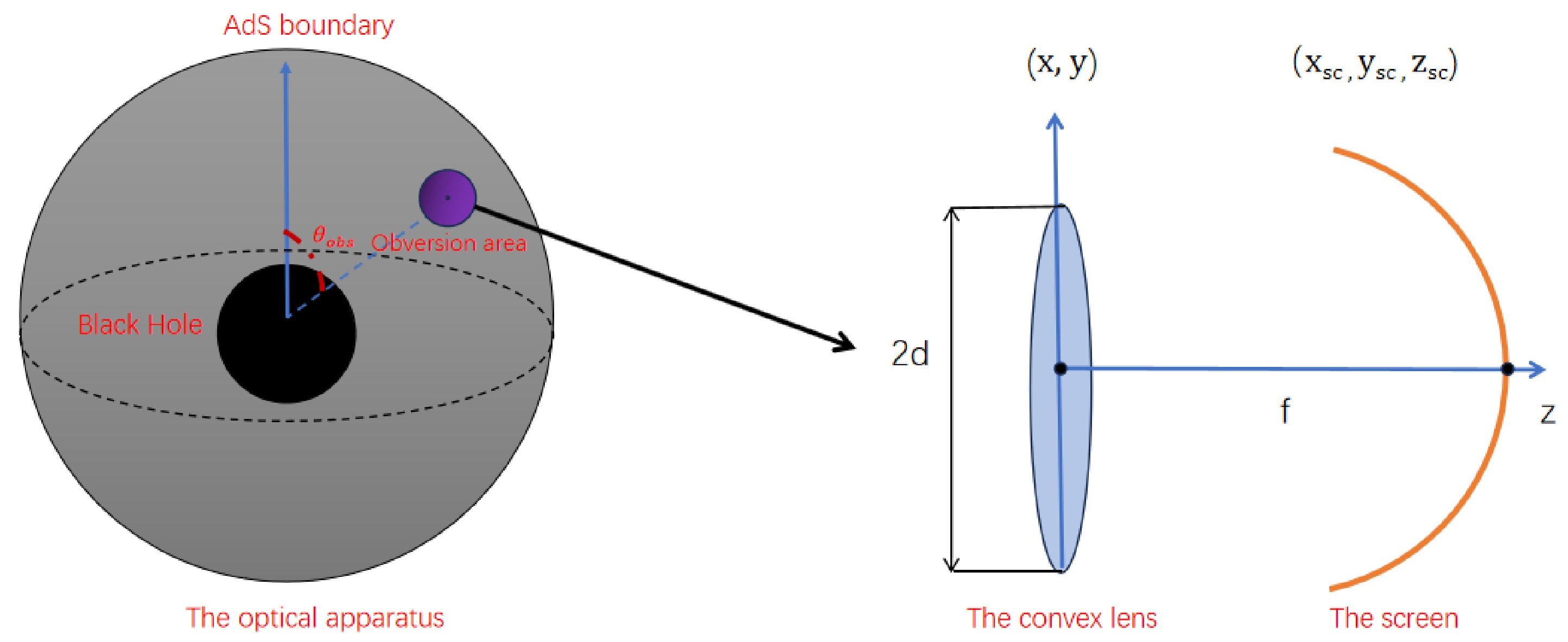

Figure 2.  (color online) Schematic diagram of the construction of the black hole image using the response function, with the observation area indicated by the purple region on the AdS boundary.

Here, $ \hat{x}=(x,y,z) $ is the Cartesian-like coordinate on the boundary $ S^2 $, and $ \hat x_{sc}=(x_{sc}, y_{sc}, z_{sc}) $ is on the screen. Eq. (5) corresponds to the Fourier transform of the response function within a specific local range. In this particular imaging system, the convex lens can be considered a converter that effectively transforms the plane wave into a spherical wave and projects it onto a curved screen. The observer is positioned at the central point of the observation area, denoted as $(\theta, \varphi)= (\theta_{\rm obs},0)$. Subsequently, we adjust the position of convex lens on the three-dimensional flat space to achieve $ (x_{cl},y_{cl})=(x, y, 0) $. The response function obtained from the observation area is projected as a planar wave onto a thin lens (referred to as the incident wave $ \Psi_{iw} (\hat{x}) $), which is then transformed by the thin lens into a spherical wave (referred to as the outgoing wave $ \Psi_{ow} (\hat{x}) $) and converges at the focal located at $ z = f $. According to the wave optics, the transformation relationship is

In principle, we require an ultra-thin convex lens with a radius d and focal length f that satisfy the condition $ f \gg d $. Subsequently, the spherical screen is located at $ (x,y,z)=(x_{sc},y_{sc},z_{sc}) $, where $ {x_{sc}}^2+{y_{sc}}^2+{z_{sc}}^2=f^2 $. The wave equation after projecting the outgoing wave $ \Psi_{ow} (\hat{x}) $ onto the screen is recorded as

where $ {\cal{N}} $ is the distance from the lens point $ (x, y, 0) $ to the screen point $ (x_{sc}, y_{sc}, z_{sc}) $. By combining Eqs. (6) and (7), we can obtain

in which $ {\cal{W}}(\hat{x}) $ represents the window function, that is

As demonstrated by Eq. (8), the wave observed on the screen can be associated with the incident wave through the application of Fourier transform within a finite domain, i.e., the range of lens size. In essence, the image of the black hole on the screen and the response function have a direct correlation.

Initially, we commence with the D-dimensional action for EPYM gravity that incorporates a non-vanishing cosmological constant. Such action is given by [63]

in which $ {\cal{R}} $ represents the Ricci Scalar, and q is a real parameter that introduces non-linearities. The term $ {\cal{F}} $ denotes the YM invariant, expressed as

and

The YM field is [71]

where $ C^{(a)}_{(b)(c)} $ represents the structure constants of the $ [\dfrac{(D-2)(D-1)}{2}]- $ parameter Lie group G. Furthermore, η represents an arbitrary coupling constant, and $ A^{(a)}_\mu $ denotes the $ SO(D-1) $ gauge group YM potentials, which are described using the Wu-Yang ansatz [72, 73]. The field equations are obtained by varying the action with respect to the spacetime metric $ g_{\mu\nu} $, which are

and

where $ G_{\mu\nu} $ is the Einstein tensor. The variation in the gauge potentials $ A^{(a)} $ leads to the YM equation, expressed as

Here, ${\bf{F}}^{(a)}=\dfrac{1}{2}F^{(a)}_{\mu \nu}{\rm d} x^\mu \wedge {\rm d} x^\nu$, ${\bf{A}}^{(b)}=A^{(b)}_\mu \wedge {\rm d} x^\nu$, and $ \star $ denotes the duality. The metric ansatz for a D-dimensional spherically symmetric line element is selected as

where ${\rm d} \Omega_{D-2}^2$ is the line element associated with a unit $ D-2 $ sphere. Depending on the dimensions D and values of q, various black hole solutions can arise from the action given in Eq. (10). Considering the condition that the power exponent $ q \neq \dfrac{(D-1)}{4} $, the metric function $ N(r) $ of a D-dimensional EPYM black hole with cosmological constant can be provided by [71]

The parameter M represents an integral constant that corresponds to the mass of the black hole, and $ Q_{\rm YM} $ denotes a charge parameter that is linked to YM fields. In the AdS spacetime, the cosmological constant is denoted as

where l is the radius of AdS spacetime. Our study focuses on four-dimensional spacetime, i.e., $ D=4 $, and the metric function in Eq. (18) can be expressed as

The power parameter q must have a positive value $ q>0 $ to ensure the fulfillment of the Weak Energy Condition (WEC) of the PYM term [63]. Additionally, the bound limit range of q is constrained to ${3}/{4} < q < {3}/{2}$, thereby satisfying certain energy conditions, including the causality condition. For $ q=1 $, the aforementioned black hole solutions can be simplified into EYM black holes [64, 65]. In this work, we consider two regions for the value of q, namely ${3}/{4} < q < 1$ and $1 < q < {3}/{2}$, to investigate whether other relevant physical quantities have the same impact on the holographic image under these two values of q. The event horizon of the black hole is located at $ r_+ $, which corresponds to the largest positive real root of $ N (r)=0 $, and we can derive the expression of the mass of the black hole in terms of the event horizon radius, that is

Now, we begin constructing a holographic model for an AdS black hole in EPYM gravity. To introduce an affine parameter ξ, such that $ \xi=1/r $, we can obtain $ N(r)=\dfrac{1}{\xi^2}N(\xi) $, and the metric Eq. (17) in the new coordinate ($ t,\xi,\theta,\varphi $) is substituted with

In this equation, ${\rm d} \Omega^2={\rm d} \theta^2+\sin \theta^2 {\rm d} \varphi^2$, and $ N(\xi) $ is expressed as

where $ \xi_+=\dfrac{1}{r _+} $ denotes the location of the black hole event horizon. The temperature of the boundary system is given by the Hawking temperature, which is

The complex scalar field Φ is considered as probe field within the system, and its dynamics can be effectively described by the Klein-Gordon equation [44], that is

in which ${\cal{D}}_\kappa=\nabla_\kappa - {\rm i} e A_\kappa$, and e represents the electric charge of the complex scalar field Φ. The utilization of Eddington coordinates enables a more efficient resolution of the Klein-Gordon equation, that is

Subsequently, the metric equation is rewritten in smooth form as

For clarity, we will set $ \mathbb{M}=-2 $ and $ e=1 $ in the subsequent analysis. The asymptotic behavior of the complex scalar field near the AdS boundary can be defined as

The terms $ {\cal{J}}_{\cal{O}} $ and $ \langle {\cal{O}} \rangle $ are the independent functions of boundary coordinates $ (\chi_e, \theta,\varphi) $ according to the AdS/CFT dictionary. In addition, $ {\cal{J}}_O $ is considered the primary source for the boundary field theory, and its corresponding expectation value of the dual operator, i.e., the response function, is determined by

Here, the chemical potential u of the boundary system is given by $ u= e \dfrac{2^{q -1} q \left(Q_{{\rm{YM}}}^2\right){}^{q }}{(4 q -3) Q_{{\rm{YM}}}} \xi _+^{4 q -3} $ under holography. Additionally, the term $ \langle {\cal{O}} \rangle $ represents the expectation value of the dual operator when the source is turned off. In the symmetry of the spacetime background, considering the source provided by Eq. (1), we can obtain the bulk solution, denoted as

The term $ Z_\zeta $ satisfies the equation of motion, that is

in which $ N'(\xi)= \partial_\xi N(\xi) $. Near the AdS boundary, the asymptotic behaviour of the $ Z_\zeta $ is expressed as

Thus, the relevant response function $ {\langle {\cal{O}} \rangle} _{{\cal{J}}_{\cal{O}}} $ is derived, which is

where

and $ \overline{\omega} $ is represented as $ \overline{\omega}=\hat{\omega}+u $. The extraction of $ \langle {\cal{O}} \rangle_{\zeta} $, which corresponds to solving Eq. (31), is crucial to obtaining the total response function $ {\langle {\cal{O}} \rangle} _{{\cal{J}}_{\cal{O}}} $. The radial equation Eq. (31) can be effectively solved by considering two crucial boundary conditions: $ {\bf{i}}) $ the AdS boundary $ Z_\zeta(0)=1 $; $ {\bf{ii}}) $ the regular boundary conditions imposed on the event horizon of the black hole $ \xi=\xi_+ $. Based on this premise, we use the pseudo-spectral method to obtain the numerical solution of $ Z_\zeta $ and derive $ \langle {\cal{O}} \rangle_{\zeta} $ [42, 43]. Considering the parameters associated with the source and spacetime structure, specifically the frequency of the Gaussian source $ \hat{\omega} $ and the power exponent q, the typical profile of the total response function $ {\langle {\cal{O}} \rangle} _{{\cal{J}}_O} $ is depicted in Figs. 3 and 4. The interference pattern results from the diffraction of the probe scalar field by the black hole in the bulk spacetime. In Fig. 3, we can observe that the amplitude of the total response function exhibits an increasing trend with increasing values of q, whereas other involved parameters are maintained at specific values such as $Q_{YM}=0.5,\; \xi_+=0.5$ and $ \hat{\omega}=80 $. When other parameters are fixed at $ Q_{YM} = 0.5,\xi_+= 0.5 $, and $ q = 7/8 $, an increase in frequency $ \hat{\omega} $ leads to a significant reduction in the amplitude of the total response function, and the period of oscillation is shortened (Fig. 4).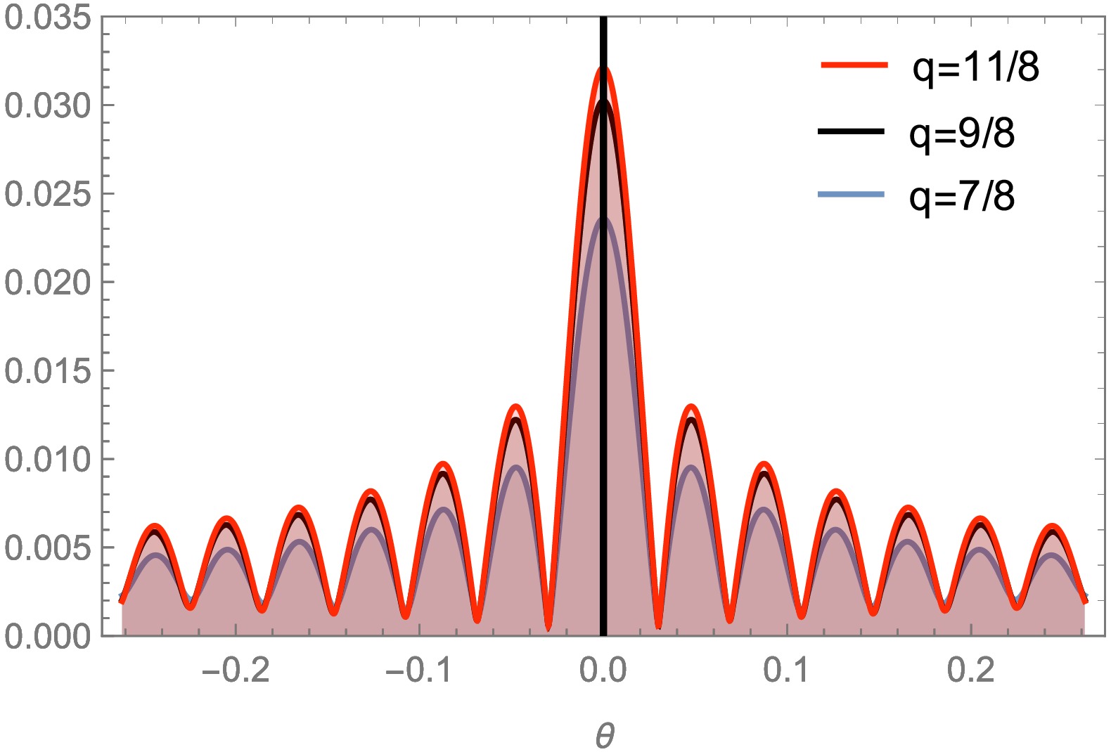

Figure 3.  (color online) Absolute amplitude of the total response function $ {\langle {\cal{O}} \rangle} _{{\cal{J}}_O} $ for different power parameters q with $Q_{\rm YM}=0.5$, $ \xi_+=0.5 $, and $ \hat{\omega}=80 $.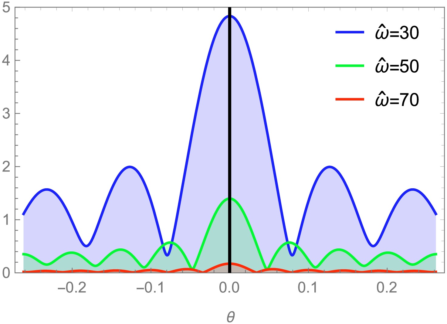

Figure 4.  (color online) Absolute amplitude of the total response function $ {\langle {\cal{O}} \rangle} _{{\cal{J}}_O} $ for different source frequencies $ \hat{\omega} $ with $ Q_{\rm YM}=0.5 $, $ \xi_+=0.5 $, and $ q=7/8 $.

Subsequently, we also manipulate the temperature T and chemical potential u of the boundary system to elucidate the changes in behavior of the total response function. The oscillation period of the wave amplitude for different values of u is depicted in Fig. 5, with specific values selected for other involved parameters as $ \xi_+ = 0.5 $, $ \hat{\omega} = 80 $, and $ q = 7/8 $. We can observe a decreasing trend in the amplitude of the total response function as the values of u increase. In Fig. 6, the amplitude of the total response function exhibits significant temperature dependence when the involved parameters are taken as $ Q_{YM}=0.5, \hat{\omega}=80 $ and $ q=7/8 $. At $ T=0.626 $, the amplitude reaches a higher peak position, followed by a significant reduction at $ T=0.513 $ and $ 0.439 $, that is, the amplitude increases with the decrease in T. The behavioral patterns of the relation $ |{\langle {\cal{O}} \rangle} _{{\cal{J}}_O}|-T $ and $ |{\langle {\cal{O}} \rangle} _{{\cal{J}}_O}|-u $ exhibit certain similarities.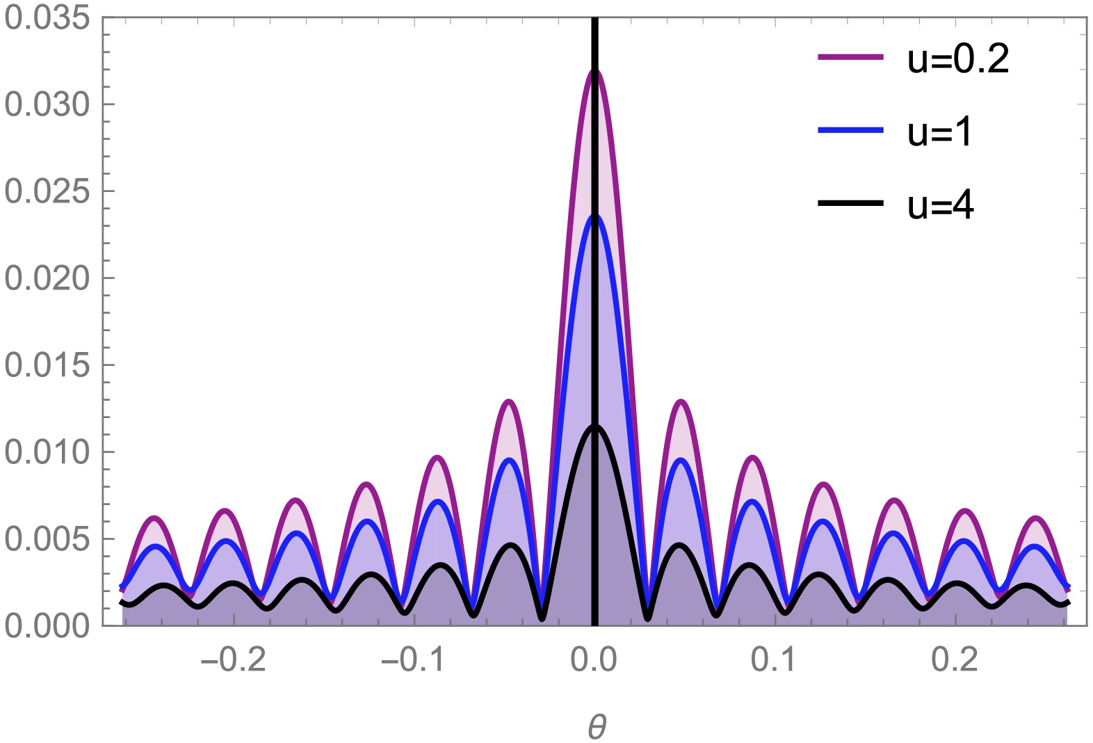

Figure 5.  (color online) Absolute amplitude of the total response function $ {\langle {\cal{O}} \rangle} _{{\cal{J}}_O} $ for different chemical potentials u of the boundary system with $ \xi_+=0.5 $, $ \hat{\omega}=80 $, and $ q=7/8 $.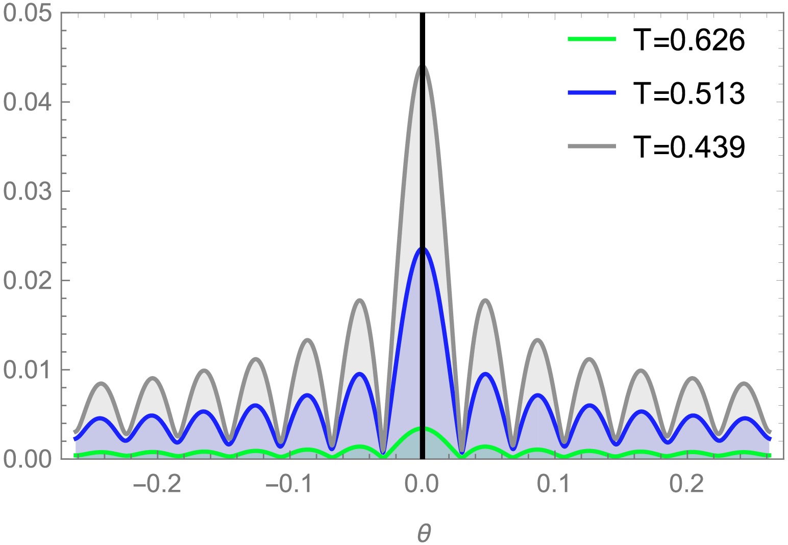

Figure 6.  (color online) Absolute amplitude of the total response function $ {\langle {\cal{O}} \rangle} _{{\cal{J}}_O} $ for different temperatures T of the boundary system with $Q_{\rm YM}=0.5$, $ \hat{\omega}=80 $, and $ q=7/8 $.

As discussed previously, the response function encompasses a wealth of spacetime information. By utilizing Eq. (8) and the virtual optical system depicted in Fig. 2, we can acquire the profiles of the dual black hole in EPYM gravity projected onto the screen. The Gaussian source, located at the south pole of the AdS boundary, should be noted. By appropriately selecting specific parameter values, we conduct numerical simulations to accurately depict the profile images of black holes and their corresponding brightness curve in Fig. 7 to Fig. 14.

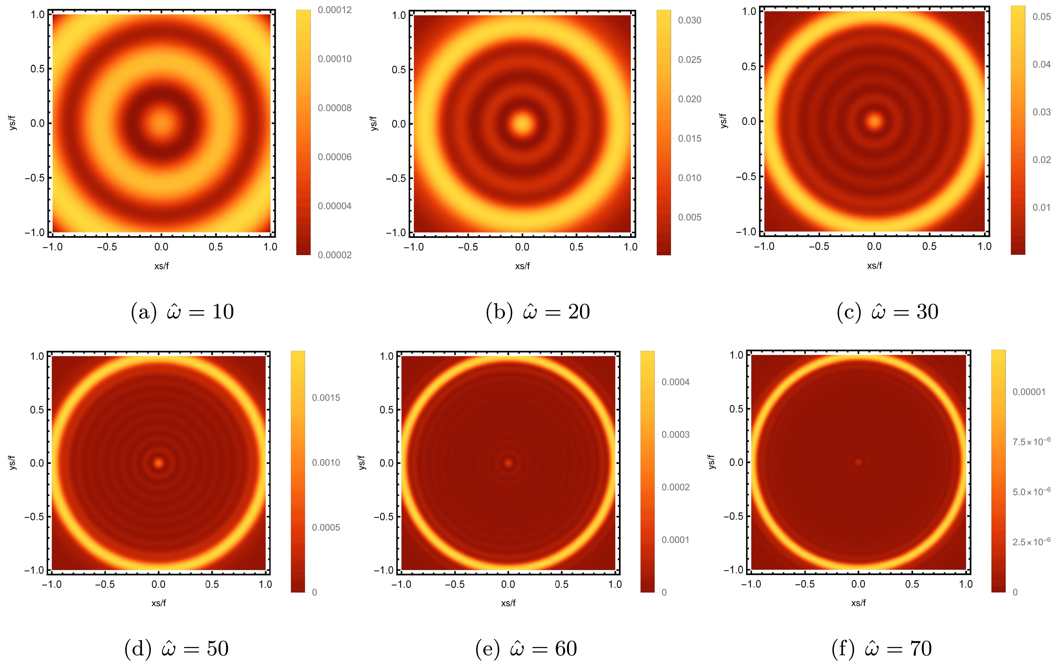
Figure 7.  (color online) Images of the lensed response observed at the observation angle $\theta_{\rm obs}=0$ for different $ \hat{\omega} $ with $Q_{\rm YM}=0.5$, $ \xi_+=0.5 $, and $ q=7/8 $.

Figure 14.  (color online) Brightness of the lensed response on the screen for different T with a fixed $ u=1 $. Here, $ \hat{\omega}=80 $, $ q=7/8 $ and from (a) to (d), the charges correspond to $ Q_{\rm YM}=0.2, 0.5, 0.8, 1.1 $ respectively.

In Fig. 7, we examine the impact of varying the source frequency $ \hat{\omega} $ on the characteristics of the holographic images observed from the north pole of the AdS boundary ($\theta_{\rm obs}=0$), whereas other relevant parameters are fixed at $ Q_{\rm YM}=0.5, \xi_+=0.5 $ and $ q=7/8 $. The results demonstrate a distinct visibility of the striped pattern, revealing a series closed axisymmetric arrangement of concentric rings. Among them, a consistently exceptionally luminous ring exists, known as the holographic Einstein ring, which corresponds to the photon ring region of the black hole in terms of geometric optics. The width of the ring decreases and becomes sharper as the value of $ \hat{\omega} $ increases.

The corresponding brightness curves of the lensed response on the screen are depicted in Fig. 8, where the y-axis and x-axis represent the intensity and position of brightness curves, respectively. The location of the bright ring in Fig. 7 corresponds to where the maximum peak of the lensed response brightness curve occurs, and variations in frequency elicit changes in the location of the maximum peak. Specifically, the increase in frequency causes the location of the maximum peak to gradually move away from the center of the screen, that is, the radius of the bright ring increases, which is consistent with the results in Fig. 7. Furthermore, the increase in frequency consistently results in a progressively steeper brightness curve, which aligns with the enhanced image sharpness depicted in Fig. 7. From this perspective, the optical appearance of the Einstein image obtained through the geometric optics approximation is highly satisfactory in the high frequency limit.

Figure 8.  (color online) Brightness of the lensed response on the screen for different $ \hat{\omega} $ with $Q_{\rm YM}=0.5$, $ \xi_+=0.5 $, and $ q=7/8 $.

We further study the effect of the power exponent q on the holographic images of the dual black hole. Given the crucial significance of q in spacetime geometry, we intend to explore the holographic images from various observation angles. In Fig. 9, the corresponding parameter values are set to $ Q_{\rm YM}=0.5, \xi_+=0.5, \hat{\omega}=80 $, and the value of q is incrementally augmented. When the observation position is located at the north pole of the AdS boundary $\theta_{\rm obs}=0$, a series of axisymmetric concentric circles rings can still be discernible in the image. As q increases, the radius of bright ring increases slightly, causing its position to shift slightly away from the center of the image, as shown in the left column of Fig. 9. Upon repositioning the observation angle to $\theta_{\rm obs}=\pi/4$, the axisymmetric bright ring dissipates and gives way to a prominent bright arc positioned on the left side of the image, as depicted in the middle column of Fig. 9. Notably, a small and less bright arc also appears on the right side of the image, exhibiting a decrease in size and luminosity as q increases. When $ q=11/8 $, the bright arc on the right side of the image essentially disappears. At the observation angle $\theta_{\rm obs}=\pi/2$, a solitary bright spot emerges solely on the left side of the image, and as q increases, the position of this bright spot progressively shifts away from the image center. Under identical parameter settings, the brightness distribution curve of the holographic image at $\theta_{\rm obs}=0$ can be obtained, as shown in Fig. 10. As q increases, the position of the maximum peak of the brightness curve shifts slightly, gradually moving away from the center. In other words, an increase in q results in an expansion of the radius of the holographic ring.

Figure 9.  (color online) Images of the lensed response observed at various observation angles for different q with $Q_{\rm YM}=0.1$, $ \xi_+=5 $, and $ \hat{\omega}=80 $.

Figure 10.  (color online) Brightness of the lensed response on the screen for different q with $ \hat{\omega}=80 $, $ Q_{\rm YM}=0.1 $, and $ \xi_+=5 $.

Subsequently, we investigate the effect of u on the images of the lensed response. These images are observed under fixed values of relevant parameters such as $\theta_{\rm obs} = 0, q = 7/8$, and $ \hat{\omega} = 80 $, are shown in Fig. 11. As the value of u increases from $ u = 0.3 $ to $ u = 7 $, the radius of the brightest ring exhibits a barely noticeable decrease but abruptly diminishes similar to a precipice when $ u=0.9 $. The same phenomenon is observed in the brightness curve of the lens response, which is shown in Fig. 12. As u increases, the peak position of the curve gradually approaches the central position, but this trend is not sufficiently pronounced, except for a notable displacement at $ u=0.9 $. The resulting Einstein ring radius is clearly dependent on u, particularly at a higher chemical potential, which is different from the result in [44]. This discrepancy occurs because the chemical potential of the boundary system is modified under the background of EPYM gravity, which naturally has a significant effect on the radius of the ring.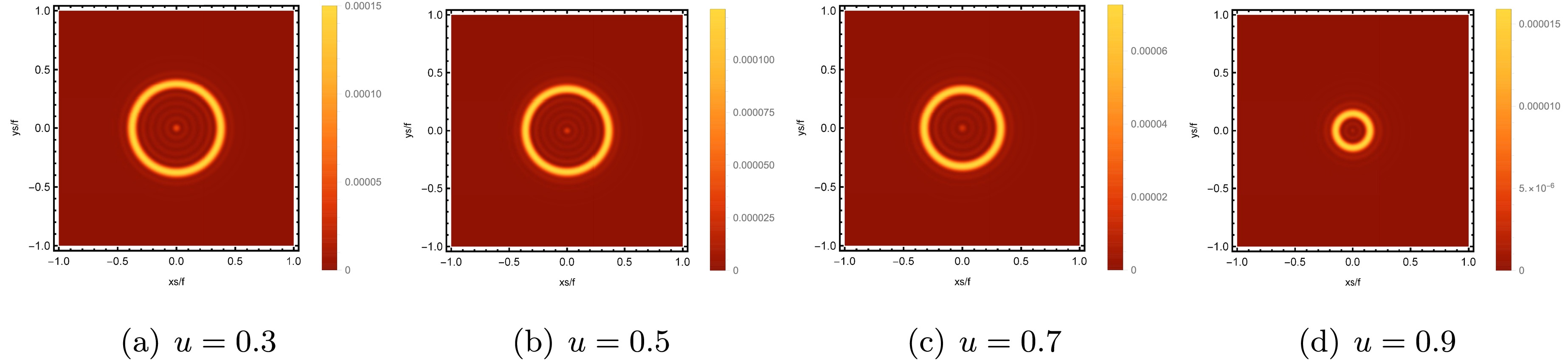

Figure 11.  (color online) Images of the lensed response observed at the observation angle $\theta_{\rm obs}=0$ for different chemical potentials u with a fixed temperature $ T=0.6 $. Here, $ \hat{\omega}=80 $ and $ q=7/8 $.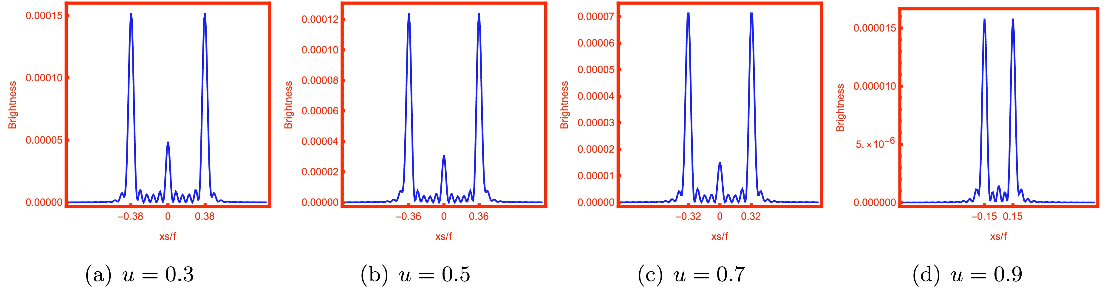

Figure 12.  (color online) Brightness of the lensed response on the screen for different chemical potentials u with a fixed temperature $ T=0.6 $. Here, $ \hat{\omega}=80 $ and $ q=7/8 $.

The variation in the image obtained at the north pole with different temperatures is plotted in Fig. 13, and the other parameters are fixed at $ u = 1 $, $ \hat{\omega} = 80 $, and $ q = {7}/{8} $. When the temperature is $ T=0.229 $, $ 0.277 $, $ 0.472 $, and $ 0.730 $, the values of the charge parameter $ Q_{\rm YM} $ in the system are $ Q=0.2 $, $ 0.5 $, $ 0.8 $, and $ 1.1 $, respectively. The radius of the formed bright ring has a visible increase as the temperature increases within the range of $ T=0.229 $ to $ T=0.277 $. In the temperature range of $ T=0.277 $ to $ T=0.730 $, although the radius of the ring has an increasing trend, it is not significant. The brightness curve of the lensed response in Fig. 14 reveals a trend of increasing distance between the maximum peak of the curve and the center of the screen, aligning precisely with the alteration in bright ring radius. The temperature dependence of the radius of the Einstein ring is evident. Specifically, at low temperatures, the radius of the ring significantly increases with an increase in temperature, which aligns with the findings in [44].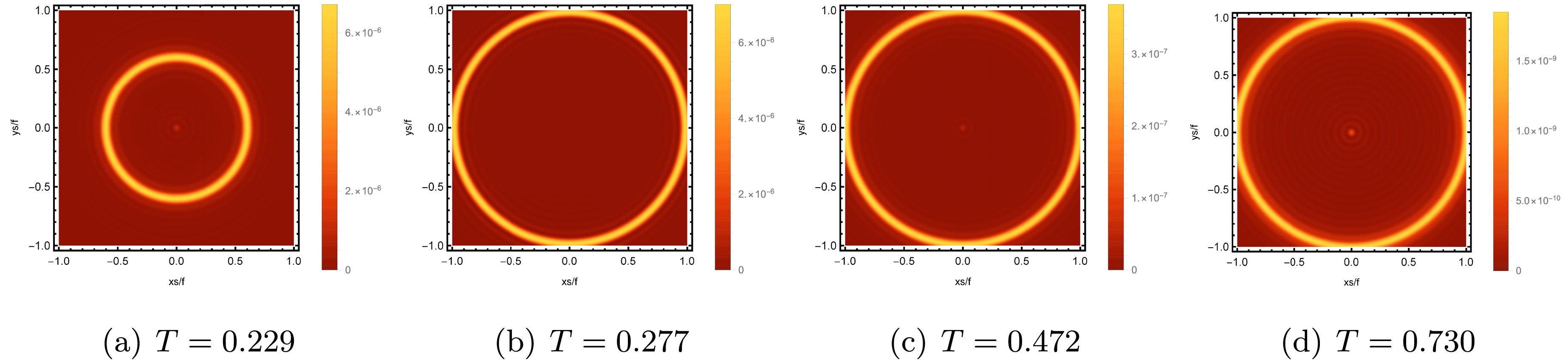

Figure 13.  (color online) Images of the lensed response observed at the observation angle $\theta_{\rm obs}=0$ for different T with a fixed $ u=1 $. Here, $ \hat{\omega}=80 $, $ q=7/8 $ and from (a) to (d), the charges correspond to $ Q_{\rm YM}=0.2, 0.5, 0.8, 1.1 $ respectively.

Following [44], the relationship between the linear response function and source can be characterized by the retarded Green function $ {\cal{G}} (t, \theta, \varphi; t', \theta', \varphi') $, that is

The retarded Green function $ {\cal{G}} $ for a weakly interacting QFT with the finite temperature or chemical potential can be expressed as

Here, $ m_T $ is the thermal mass and can be expressed as

where the correction term $ h(T,u) $ is

The parameter α represents the inverse of temperature, given by $ \alpha=\dfrac{1}{T} $, and $ \hat{\omega}_\varsigma=\sqrt{m^2+\varsigma(\varsigma+1)} $. The variation tendency of h enables us to qualitatively determine the response or ring radius. Thus, we present the typical h dependence on T and u inFig. 15.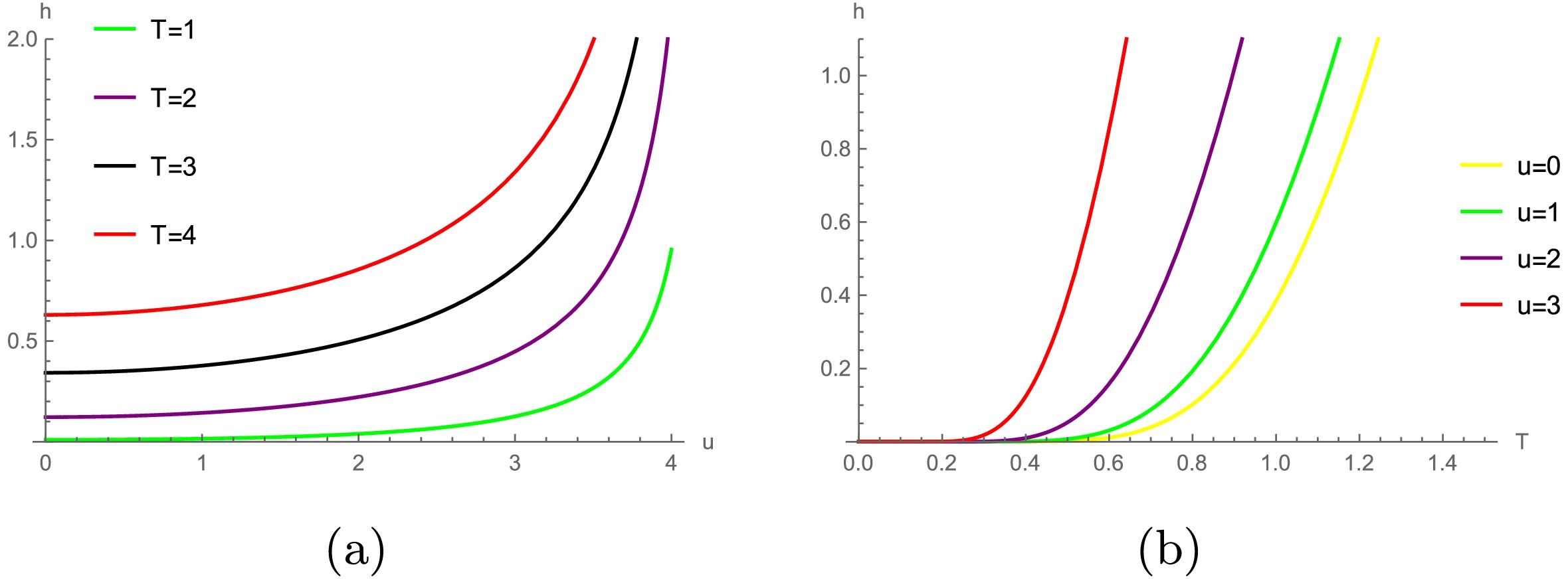

Figure 15.  Dependence of $ h(t,u) $ on the temperature and chemical potential with $ m^2=-2 $.

As depicted in Fig. 15 (a), for a given chemical potential, an increase in T leads to an increase in the value of h, and the radius of the corresponding ring increases. The value of h increases over a very small interval in the temperature range of $ 0<T<1 $, indicating that the change in the radius of the ring within this temperature range will not be significant. These results are consistent with those shown in Fig. 13. From Fig. 15 (b), the variation in h is negligible for the chemical potential $ 0<u<1 $ in a low temperature range, which is consistent with that obtained in Fig. 13. However, at a fixed T, the value of h increases with a larger u, indicating that the radius of the ring should correspondingly increase. This does not match the results shown in Fig. 11.

Regarding the shadow image of a black hole, the luminous ring depicted in the image corresponds to the location of the photon ring of the black hole. To understand the physical significance of the holographic Einstein ring further, we analyze the correlation between the bright ring in the image and the photon ring surrounding a black hole from a geometric optics perspective. We can employ the Eikonal approximation as it transforms the Klein-Gordon equation into the form of Hamilton-Jacobi equation, denoted by

where $ {\cal{I}} $represents the action. In the system (17), the above equation can be expressed as

The spherically symmetric structures in Eq. (17) enable us to always position the photon orbits on the equatorial plane, simplifying the model without sacrificing generality, i.e., $ \theta=\dfrac{\pi}{2} $ and $ \dot\theta=0 $. This spacetime contains two killing vectors, ω and L, enabling us to express the action as

and

Here,

ω and L denote the conserved energy and angular momentum, respectively. The path of photon propagation will be described by the aforementioned conditions. Thus, the ingoing angle $ \theta_{in} $ [44] with the normal vector of boundary $ \mathfrak{n}^\gamma =\dfrac{ \partial}{\partial r^{\gamma}} $ is defined as

We can also obtain

Hence, the ingoing angle $ \theta_{in} $ of photon orbit from the boundary is determined as

The photons in close proximity to the photon ring will orbit around the black hole one or more times, resulting in cumulative luminosity within this region. The photons that can be located in the vicinity of the photon ring also apply to Eq. (46), and the corresponding diagram is shown in Fig. 16. Here, the angular momentum of these photons is denoted as $ L_S $, and their light trajectory satisfies the following conditions: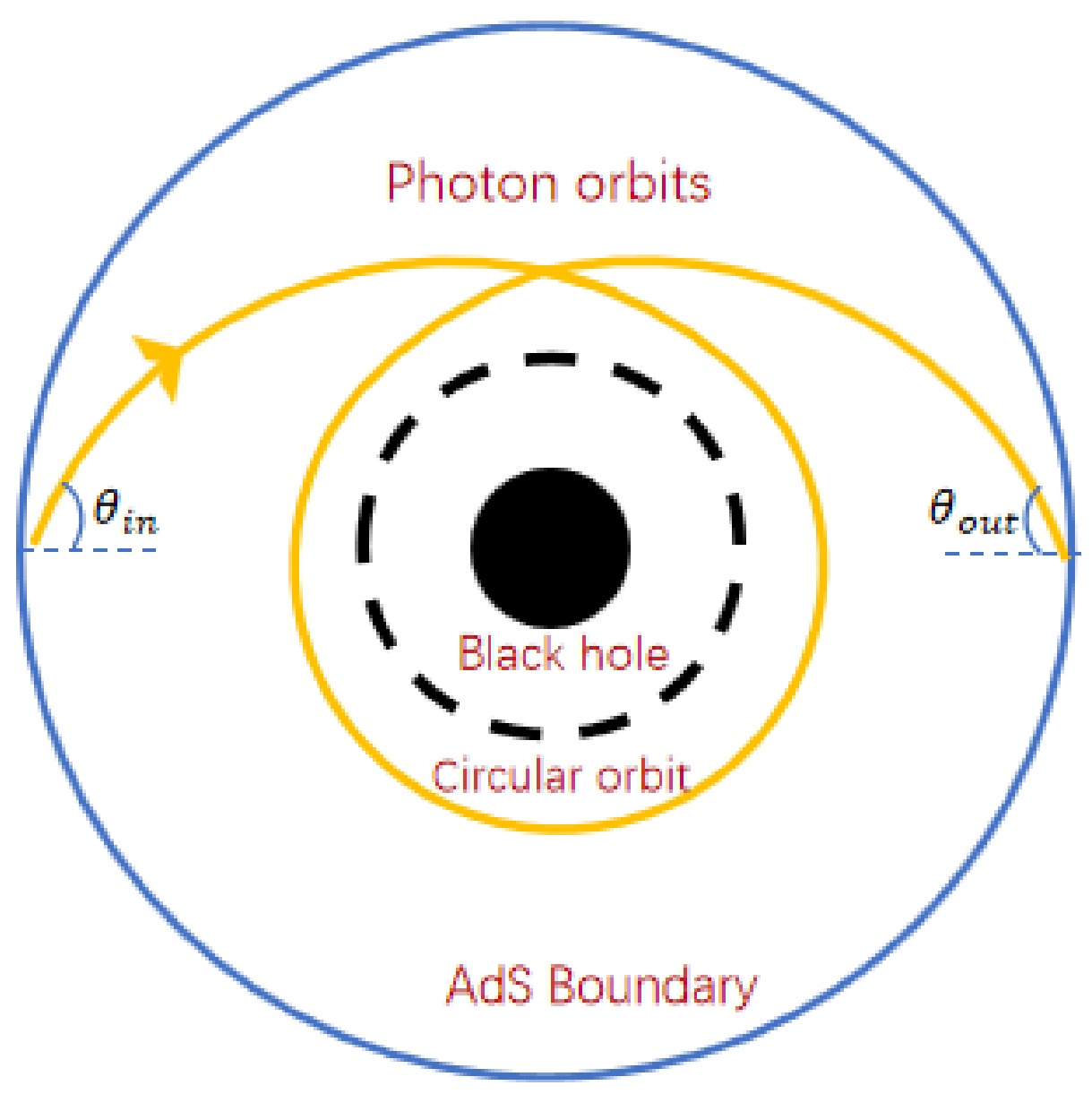

Figure 16.  (color online) Ingoing and outgoing angles of the photon at the photon ring.

From the perspective of geometric optics, the angle $ \theta_{in} $represents the angular displacement of the incident ray's image from the zenith when an observer positioned on the AdS boundary gazes upwards into the AdS bulk. In a scenario where the entry and exit points of photon trajectories on the AdS boundary align precisely with the center point of the black hole, the radius of the ring image observed by an observer corresponds to the incidence angle $ \theta_{in} $ owing to axial symmetry. Additionally, the Einstein ring is formed on the screen, as shown in Fig. 17, with the ring radius as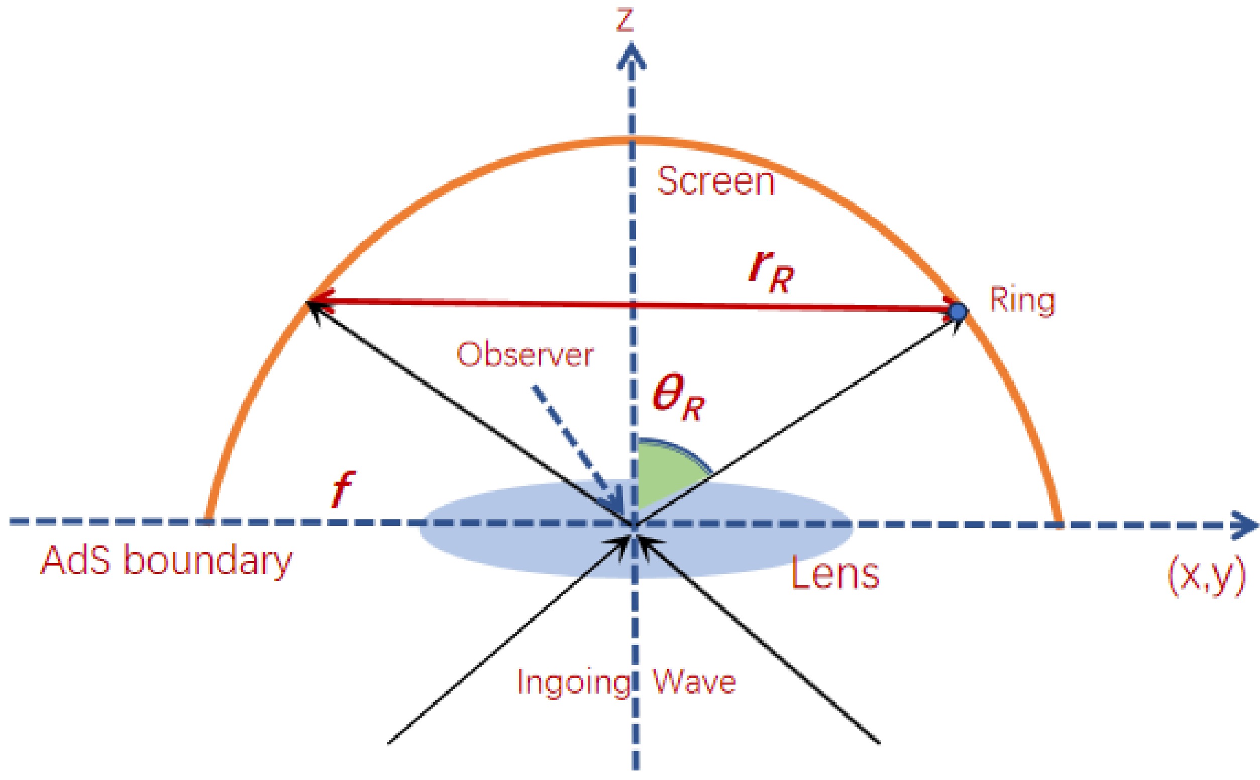

Figure 17.  (color online) Relation between $ \theta_R $ and $ r_R $.

According to [42, 43], we can obtain $ \sin \theta_{R}= \sin \theta_{in} $ for a sufficiently large ς, which means that

and the focal length f of the lens here determines the degree of magnification. Therefore, the radius of the holographic ring corresponds to the size of the photon ring. In essence, the incident angle of the photon and the angle of the photon ring both refer to the angle of the photon ring that the observer can observe, and they should be basically equivalent. Moreover, we validate this relationship through a numerical calculation. In Figs. 18 and 19, the radius of the Einstein ring is depicted for different values of q, where $ r_R/ f $ represents the ring radius as a function of temperature and chemical potential. The red data points consistently cluster around the blue curve, exhibiting values within a three percent margin of each other. The Einstein ring angle obtained in the holographic analysis is consistent with the ingoing angle derived from geometric optics, thus demonstrating a high level of agreement between the two approaches.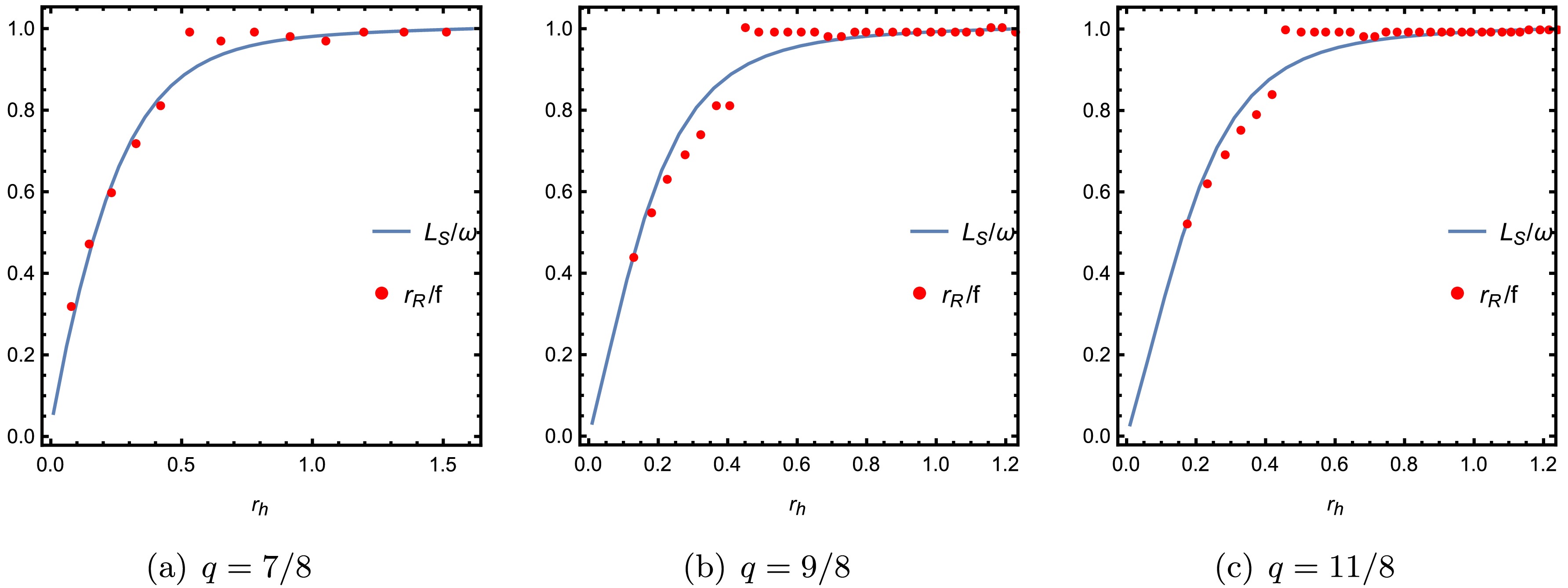

Figure 18.  (color online) Comparison of the results obtained using wave and geometric optics for different q with a fixed chemical potential $ u=1 $.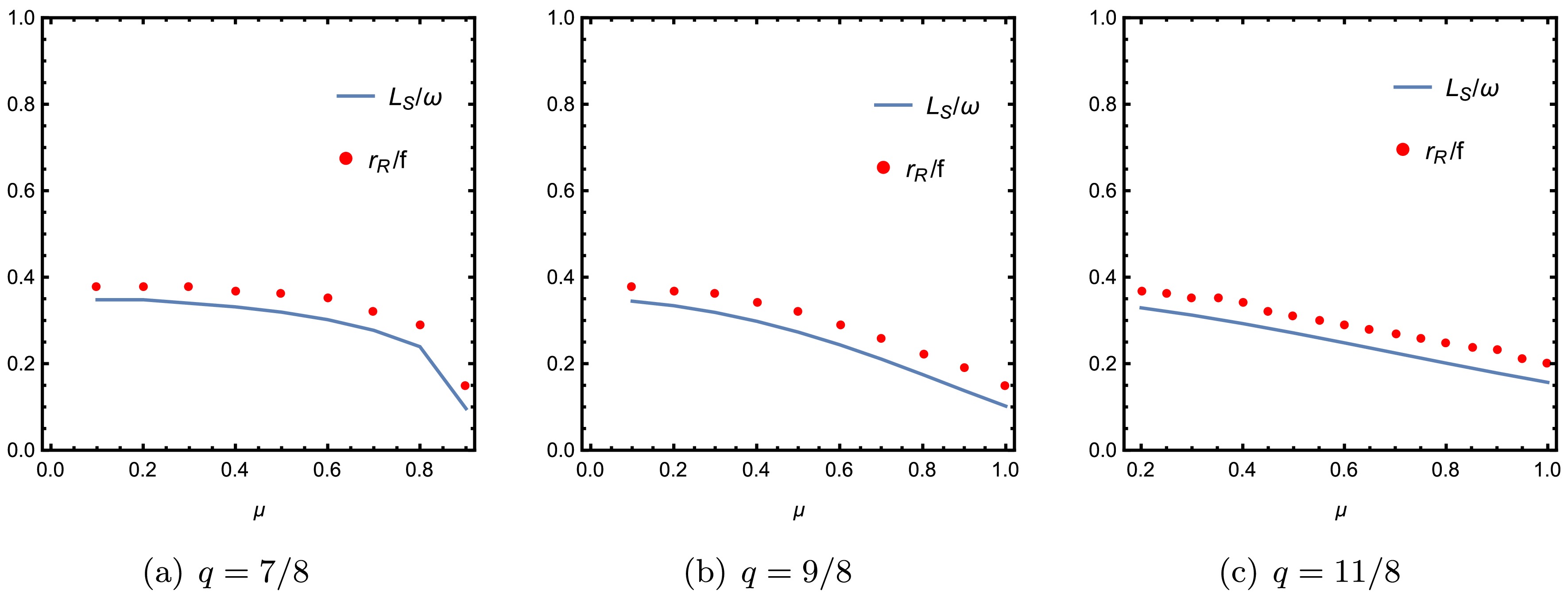

Figure 19.  (color online) Comparison of the results obtained using wave and geometric optics for different q with a fixed temperature $ T=0.6 $.

Gravitational lensing, a prevalent optical phenomenon in the universe, is a paramount research tool and pivotal phenomenon in astrophysics. It has a significant role in cosmology, encompassing dark matter, dark energy, large-scale gravity, and exoplanet detection. As one of the most vivid demonstrations of gravitational lensing, Einstein rings offer an abundance of valuable insights into the intricate fabric of spacetime. From this perspective, we employ wave optics to investigate the holographic image of an AdS black hole within the EPYM gravity framework. The AdS boundary is equipped with an oscillating Gaussian source, and the scalar wave emitted from this source propagates through the bulk spacetime, resulting in a corresponding lensed response on the opposite side of the boundary. The diffraction pattern of the total response function $ {\langle {\cal{O}} \rangle} _{{\cal{J}}_{\cal{O}}} $ is always present during scalar wave propagation through the black hole, as revealed by extracting the local response function at the boundary. The characteristics of the absolute amplitude of the total response function, for various values of the involved parameters, are depicted in Fig. 3−Fig. 6. These figures demonstrate the change in wave oscillations in response to variations in state parameters. Fig. 3 shows that, with an increase in the power exponent q, the amplitude peak of $ {\langle {\cal{O}} \rangle} _{{\cal{J}}_{\cal{O}}} $ exhibits a steady increasing trend. However, as the frequency of the wave source increases, the amplitude peak of $ {\langle {\cal{O}} \rangle} _{{\cal{J}}_{\cal{O}}} $ diminishes, and the time period of the scalar wave shortens (Fig. 4). Furthermore, the impacts of the finite chemical potential u and horizon temperature T on the amplitude of the total response function are shown in Fig. 5 and Fig. 6. The elevation in T and u progressively diminishes the corresponding amplitude of the response function. However, the reduction is more pronounced with variations in T.

Although the diffraction pattern of the response function is analyzed, it does not intuitively provide specific information about the black hole. By utilizing a virtual optical system consisting of a convex lens and a spherical screen (note that this optical system is in neither the bulk spacetime nor the boundary), we can capture the holographic image of an AdS black hole in EPYM gravity. In all scenarios, irrespective of the specific parameters involved, when the light source is located at the south pole, an observer located at the north pole ($\theta_{\rm obs}=0$) will invariably perceive an image manifesting as a luminous, axisymmetric ring, commonly referred to as the holographic Einstein ring. Variations in the relevant parameters exhibit distinct impacts on specific attributes of the ring, such as its size and brightness. In Fig. 7, we observe that, as the value of ω increases, the width of the ring becomes progressively narrower and more sharply defined, whereas the radius of the ring exhibits a decreasing trend. Additionally, the brightness curve of the response function is provided, where the maximum peak on the curve corresponds to the position of the bright ring (Fig. 8). The results demonstrate that as frequency increases, the position of the maximum peak progressively shifts away from the center of the screen. In other words, the radius of the bright ring expands, which is consistent with the findings presented in Fig. 7. Interestingly, in low frequency bands, an increase in frequency leads to an increase in observed brightness, whereas in high frequency bands, an increase in frequency leads to a decrease in observed brightness. In Fig. 11, we analyze the influence of u on the obtained images of AdS black hole in EPYM gravity. The results indicate that the radius of the ring decreases as u of the boundary system increases. However, this decrease is relatively insignificant at low chemical potentials ($ 0.3<u<0.5 $) and becomes more pronounced as the chemical potential reaches higher values ($ 0.7<u<0.9 $), which is different from the effect of chemical potential on ring radius in [44]. Owing to the chemical potential of the boundary system is modified under the background of EPYM gravity, the impact of changes in chemical potential on the radius of the resulting ring is emphasized. Fig. 12shows that the brightness curve of the lensed response on the screen, corresponding to different u values, exhibits a gradual decrease in the intensity of the observable ring brightness as u increases. The impact of boundary system temperature T variation on the ring is contrary to that of chemical potential, that is, the radius of the ring increases when the temperature increases, particularly at low temperatures. The influence of temperature on the ring radius is consistent with the results in [44].

Considering the dependence of spacetime on q, we also investigate the effect of the change in q on the Einstein ring at different observation angles ($\theta_{\rm obs}=0, \pi/4, \pi/2$), as shown in Fig. 9. As depicted in the leftmost column of Fig. 9, when the observation angle is $\theta_{\rm obs}=0$, the image of the black hole appears as a bright ring with a series of concentric stripes, which correspond to the diffraction behavior of the total response function. Thus, the radius of the bright ring in the image is observed to increase with increasing q, and the same conclusion can be obtained from the brightness curve in Fig. 10. When the observation angle is $\theta_{\rm obs}=\pi/4$, as shown in the middle column of Fig. 9, the ring structure in the image becomes disrupted, leaving a bright arc visible on the left side of the image, whereas the right side exhibits a smaller and less intense arc. The bright arc on the left side remains unaffected as q increases, but the bright arc on the right side gradually diminishes. In the rightmost column of Fig. 9, the observation angle is $\theta_{\rm obs}=\pi/2$, the bright arc disappears and only one bright spot is located on the left side of the image. As q increases, the position of the spot tends to move away from the center of the image. Moreover, the observable brightness of the resulting image decreases as q increases, regardless of any changes in the observation angles.

We end by comparing the results between the bright ring obtained within the holographic framework and the position of the photon ring of black hole obtained through geometric optics. In Figs. 18 and 19, the radii of the photon ring (depicted by the blue curve) and Einstein ring (represented by discrete red dots) are plotted as functions of varying q values. As anticipated, the ingoing angles of the photon ring consistently align numerically with those of the Einstein ring across varying T and u values. Hence, a correlation can be established between the positions of the photon ring and holographic Einstein ring, thereby affirming the reliability of wave optics within the holographic framework. In addition, holographic images can serve as a crucial tool for discerning the geometric characteristics of different black holes and provide specific insights into the phenomenological consequences of black hole dynamics, particularly when considering fixed wave sources and optical systems. We hope that these discoveries will provide a more vivid and intuitive understanding of Einstein rings and their associated phenomena, thereby facilitating future tabletop experiments.