Full next-to-leading order calculations for dark matter pair production in the leptoquarks plus dark matter model

Over the past decade, observations of $ R_{K^{(*)}} $ and $ R_{D^{(*)}} $ through the LHCb, Belle, and BaBar collaborations have provided evidence for Lepton Flavour Universality Violation (LFUV) [1−14]. Based on the Standard Model (SM) theorem, the introduction of leptoquarks (LQs), which directly couple a quark to a lepton through Yukawa-type interactions, provides an alternative path to explain LFUV [15−18]. The ATLAS and CMS collaborations at the large hadron collider (LHC) have determined the LQ mass range to be approximately 1.0−1.8 TeV [19−30], extending to 1−2 TeV when suppressing the channels that couple to first-generation leptons [31−33]. Recently, Ref. [34] presented a systematic description of the complete Lagrangian and the corresponding sets of Feynman rules for scalar LQs. The coupling strengths between LQs and SM fermions have been fitted in the LO and NLO by Refs. [35−37]. To search for LQ signals from a theoretical perspective, several phenomenological calculations for LQ production at colliders have been performed [38−45]. The next-to-leading order (NLO) QCD corrections for scalar LQ pair production have been calculated in Refs. [46, 47] and matched with parton showers in Refs. [48−53]. Furthermore, the DM can be explored by extending the LQ model further, as discussed in Refs. [54−62]. Reference [62] establishes a connection between flavor anomalies and the dark sector by implementing the scalar LQs $ (S_1) $ as a mediator to the dark sector ($ \chi_1, \chi_0 $). Here, $ \chi_0 $ denotes the lightest and neutral DM candidate. This model provides the following rich opportunities for new physics (NP) research: i) The introduction of $ S_1 $ provides a minimal framework to study the $ R_{D^{(*)}} $ anomalies, which involve interactions between second- and third-generation quarks and third-generation leptons. ii) Another aspect is the search for NP in the missing transverse energy channel, where NP signals can be detected in processes that involve the production of a pair of $ \chi_1 $ particles, with $ \chi_1 $ cascade decaying to $ \chi_0 $ and SM fermions. iii) Searches are conducted for the production of LQ pairs and their visible decays. The signal for LQs can be approached through the production of $ S_1 $ pairs, with $ S_1 $ decaying into SM fermions. iv) Another important search involves LQs plus DM. For this signal, it provides an opportunity to explore the relationship between the dark sector and the visible decay of LQs. We can explore this relationship by producing a heavy $ S_1 $ pair, where one $ S_1 $ decays into a muon and a charm or strange quark, while the other decays into a $ \chi_1 \chi_0 $ pair, with $ \chi_1 $ further decaying into $ \chi_0 $ and SM fermions. The allowed parameter space for this model is determined by considering various experimental constraints, including collider searches for LQs and missing energy signals, as well as cosmological limits such as direct detection and DM relic abundance. Therefore, this model, which describes LQs and DM, is worth exploring further.

In this study, following the Lagrangian proposed by Ref. [62], we calculate the full NLO (EW+QCD+ISR) corrections for $ \chi_1 \bar{\chi}_1 $ pair production, followed by $ \chi_1 $ cascade decay into stable DM and SM final states. Compared to hadron colliders, lepton colliders provide a clearer background for searching for NP signals. In the analysis of Ref. [62], DM masses are restricted to a heavy range that is larger than the center-of-mass (COM) energies of most electron–positron colliders, except for the compact linear collider (CLIC) [63−65]. Furthermore, muon colliders [66−76] have great potential for exploring BSM signatures, with COM energies that could exceed 10 TeV. Recently, the phenomenology of muon colliders has received increasing attention. For instance, BSM signals, including NLO corrections [89, 90], have been explored at muon colliders by Refs. [76−88] . Therefore, muon colliders can be used strong candidates for high $ \sqrt{s} $ lepton colliders. In this study, we analyze leptons + $\not {E}_T$ (+ jets) processes at CLIC and muon colliders.

This paper is organized as follows: In Sec. II, we briefly describe the LQs plus DM model and present the benchmark points used for calculations after applying the constraints. We provide a brief description for the $ \chi_1 \to \chi_0 l q $ decay and the scan of the decay branching ratios for $ \chi_1 $. In Sec. III, we detail the calculations of leading order (LO) and NLO QCD and EW corrections for $ \chi_1 \bar{\chi_1} $ pair production. We verify the reconstruction of the LQs+DM model using $ {\mathrm{Lanhep}}$, which includes the renormalization of masses and fields under the on-shell (OS) scheme. Moreover, we perform some numerical checks for ultraviolet (UV) and infrared (IR) finiteness and present the results of NLO EW and QCD corrections. Moreover, IR singularities are regularized using the mass regularization scheme and subtracted employing the dipole subtraction [91−93] and two cutoff phase-space slicing methods [94]. We examine the dependence of the results on parameters to ensure proper subtraction of IR divergences, serving as an additional validation for our calculations. In Sec. IV, we analyze the signals for $ \chi_1 \bar{\chi}_1 $ pair production, cascade decay to $ \chi_0 lq $, and the relevant backgrounds. In Sec. V, we first present the results of the NLO correction factors for $ \chi_1 \bar{\chi}_1 $ pair production and then provide the results for signal significance at LO. Based on differential distributions, we discuss the kinematic cuts that improve signal significance and present results after applying these cuts. Furthermore, we evaluate signal significance considering NLO correction factors and kinematic cuts. Finally, we provide a brief summary in Sec. VI.

Following Ref. [62], the Lagrangian describing the phenomenology of LQs plus DM is established as

Where $ S_1 $ denotes a single scalar LQ, which is employed as a mediator to associate the dark sector ($ \chi_1, \chi_0 $). $ \chi_1 $ and $ \chi_0 $ (lightest) denote Dirac and Majorana fermions as DM candidates, respectively. The antiparticle of $ \chi_1 $ is itself, and $ \chi_1 $ and $ \chi_0 $ obey the odd transformation under the $ \mathbb{Z}_2 $-type symmetry. Under the SM gauge group, $ \chi_1 $ and $ S_1 $ share the same representation as (3, 1)$ _{-1/3} $. Meanwhile, $ \lambda_{(R,L)} $ and $ y_{DM} $ are free parameters describing the coupling strength of LQs with SM leptons and quarks and with the dark sector, respectively.

This model, as described in Eq. (1), can be characterized by six (dimension) independent parameters $\{M_{S_1}, ~M_{\chi_1}, M_{\chi_0}, ~ \lambda_R,~ \lambda_L, y_{DM} \}$. These parameters are limited by experimental data from cosmology and the LHC. We provide a brief description of these constraints as follows:

● Missing energy searches. The $ \chi_1 \to \chi_0 lq $ decay allows searches for leptons, jets, and missing energy in LHC. The allowed parameter space can be determined by reinterpreting the signatures of missing energy production associated with $ b \bar{b} $ pair [23], mono-jet [95, 96], heavy-flavour jets [97], $ \tau^+\tau^- $ pair [98], and soft leptons [99]. $ M_{S_1} $ is constrained to be greater than $ 1.6 $ TeV for $ \lambda_L> \lambda_R $ and $ M_{\chi_1} > 800 $ GeV. By contrast, for $ \lambda_R> \lambda_L $, the $ M_{S_1}\in[1.4,1.5] $ TeV region is allowed for $ \Delta M \in[5,30] $ GeV and $ \Delta M = M_{\chi_1}-M_{\chi_0} $. The range of $ \Delta M $ could be extended to $ [50,100] $ GeV for $ M_{S_1} > 1.4 $ TeV.

● Leptoquark searches. At the LHC, LQ pair production can be explored through signatures of SM final-state processes, such as $ t\tau t\tau $ [100], $ b\nu b\nu $ [23], and $ b\nu t\tau $ [101]. The signatures of single LQ production in association with a lepton, for example, the $ t\tau \nu $ production [24, 28], can be used to restrict the input parameters of the model. By reinterpreting these signatures, we can determine the allowed parameter space.

● Dark matter direct detection. The scattering of DM $ \chi_0 $ off nucleons is constrained by existing constraints from Xenon1T and proposed DARWIN [102] experiments. In the perturbative region allowed by the missing energy searches at the LHC, the Xenon1T results become insensitive to the model parameters. The DARWIN experimental results will be restricted to $ y_{\chi} < [3,5] $ for different values of $ M_{\chi_1} $ and $ M_{\chi_0} $.

● Dark matter relic density. The relic density of dark matter can be generated through the standard freeze-out and the conversion-driven freeze-out regime (CDFO) mechanisms for the model described in Eq. (1). As $ y_\chi $ increases, the relic density $ \Omega h^2 $ decreases, whereas it increases with $ \Delta M $. When the Planck data $ \Omega h^2 = 0.12 $ [103] are satisfied, for $ \lambda_L> \lambda_R $, smaller $ y_{\chi}\in [10^{-5}, 10^{-4}] $ becomes a candidate for CDFO solutions. For the $ \lambda_R > \lambda_L $ case, $ y_\chi $ is constrained to $ [10^{-5}, 10^{-1}] $ for $ \Delta M \in [50,100] $ GeV and can be enlarged to $ y_{\chi} >1 $ for larger $ \Delta M $.

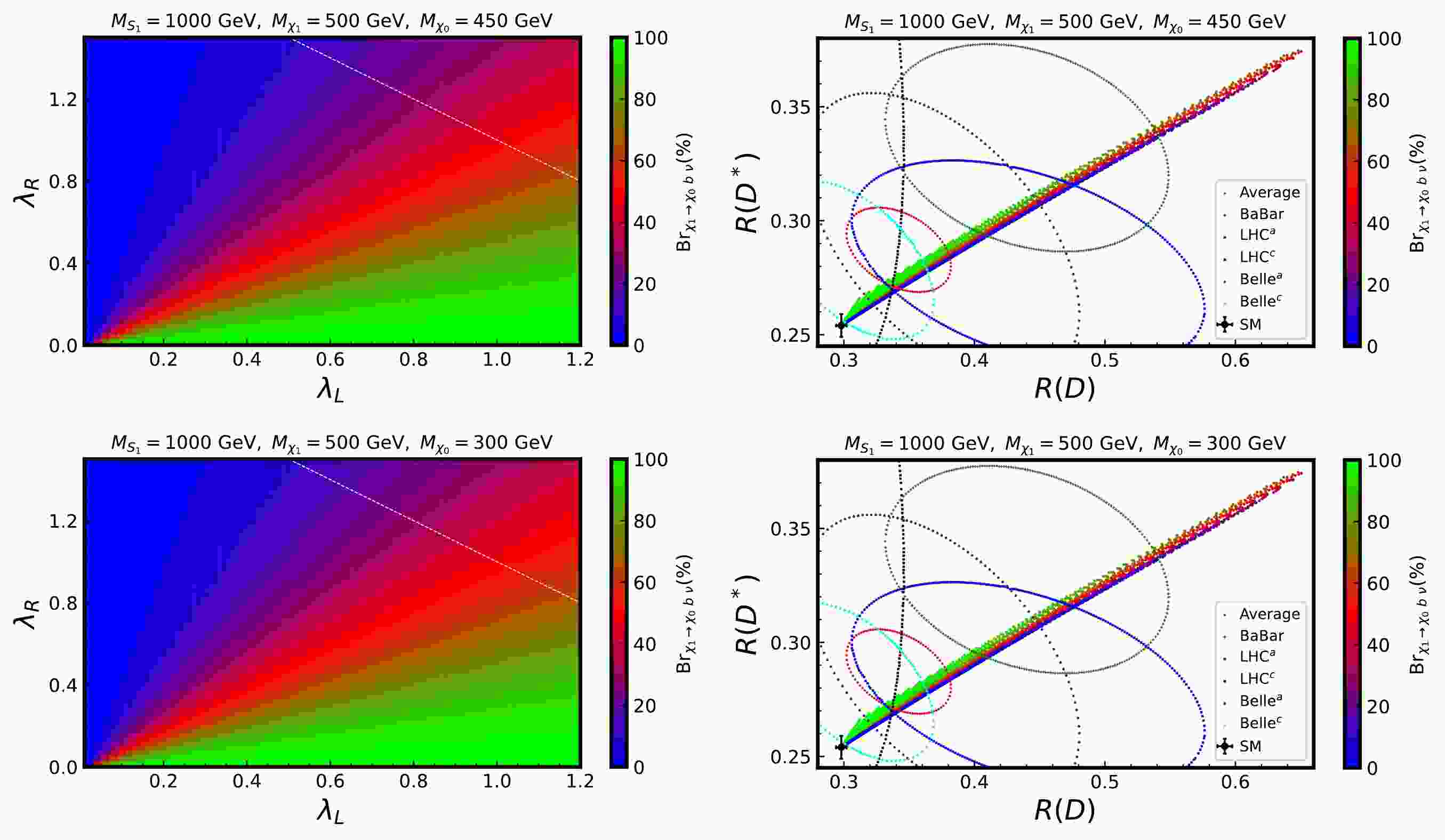
Following Ref. [62], we adopt a minimal framework for LQs, where only $ (\lambda_L)_{33} = \lambda_L $ and $ (\lambda_R)_{23} = -\lambda_R $ are non-zero. In Table 1, we use the four benchmark points (BPs) proposed by Ref. [62] for our calculations, which satisfy the constraints from cosmology and the LHC. For the first two BPs in Table 1, where $ \lambda_L > \lambda_R $, $ \chi_1 $ decays predominantly into the $ \chi_0 b \nu_{\tau} $ final state. $ \lambda_L < \lambda_R $ leads to $ \chi_1 \to \chi_0 c \tau $ being a dominate channel for BP3 and BP4. However, the $ \chi_1 \to \chi_0 t \tau $ channel is negligible for BP3, even though it is kinematically allowed $ \Delta M > M_t + M_{\tau} $. To perform the signal analysis, as shown in Fig. 1, we first present a scan for the branching ratios of $ \chi_1 $, with the upper and lower panels corresponding to $ \Delta M $ = 50 and 200 GeV, respectively. In the left panel, we consider the region $ 0<\lambda_L<1.2, 0<\lambda_R<1.5 $, and the white lines represent the contour $ \lambda_L + \lambda_R = 2 $. The $ \chi_0 t \tau $ channel is open for the $ \Delta M = $200 GeV case; however, its branching ratio is very small compared to the other two channels. This finding indicates that the results of $ \chi_0 c\tau $ are symmetric to those for $ \chi_0 b\nu_\tau $ around $ \lambda_L = \lambda_R $; thus, we do not show them here. Moreover, in the right panel, we map the scan results to those of the $ R(D)-R(D^*) $ plane, along with the experimental results with $ 65 $% CL and combination from HFLAV [104]. Larger values of $ \lambda_{L/R} $ result in larger values of $ R(D^{(*)}) $; thus, we exclude the region of $ \lambda_L + \lambda_R>2 $ in the right panel. Meanwhile, we observe that the results of $ R(D^{(*)}) $ degenerate to the SM for $ \lambda_L = \lambda_R = 0 $. Fig. 2 shows the results of Br$ _{\chi_1 \to \chi_0 lq} $ as a function of $ M_{\chi_0} $. As shown in the left figure of Fig. 2, with an increase in $ \Delta M $, the $ \chi_0 b\nu_{\tau} $ channel gradually becomes dominant. However, the branching ratios are independent on $ \Delta M $ for $ \Delta M > 50 $ GeV. From the right case of Fig. 2, the $ \chi_0 c \tau $ channel decreases as $ \Delta M $ increases.

	$M_{S_1}$/GeV	$M_{\chi_1}$/GeV	$M_{\chi_0}$/GeV	$\lambda_L$	$\lambda_R$	$y^{DM}$	Br$_{\chi_1 \to \chi_0 c\tau}$ (%)	Br$_{\chi_1 \to \chi_0 b \nu_\tau}$ (%)
BP1	1700	850	840	1.19	0.51	$10^{-4}$	29.66	70.34
BP2	1700	1030	950	1.19	0.51	1	15.64	84.35
BP3	1500	800	600	0.36	1.5	3	94.57	5.43
BP4	1500	800	700	0.36	1.5	0.5	94.59	5.41

Table 1.  Benchmark points are selected to perform calculations.

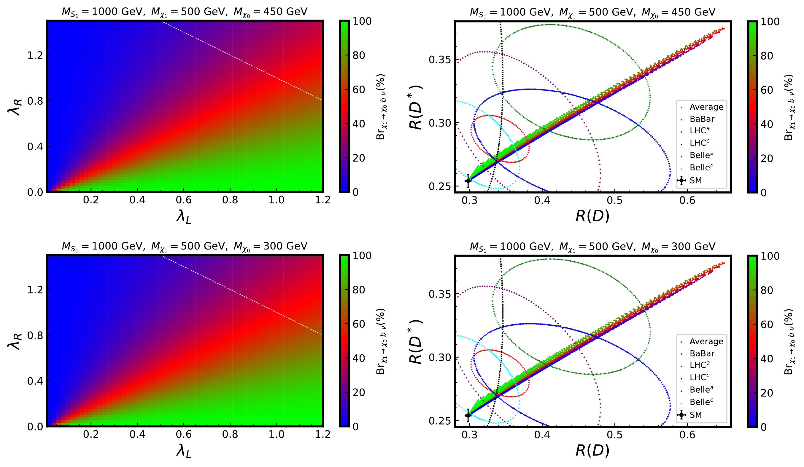
Figure 1.  (color online) Branching ratios of $\chi_1$ in the $\lambda_L-\lambda_R$ and $R(D)-R(D^*)$ planes are shown in the left and right panels, respectively. The upper and lower panels correspond to $\Delta M = 50$ and 200 GeV. In the left panel, the white lines denote the contour $\lambda_L + \lambda_R = 2$ and the region where $\lambda_L + \lambda_R > 2$ has been excluded in the right panel.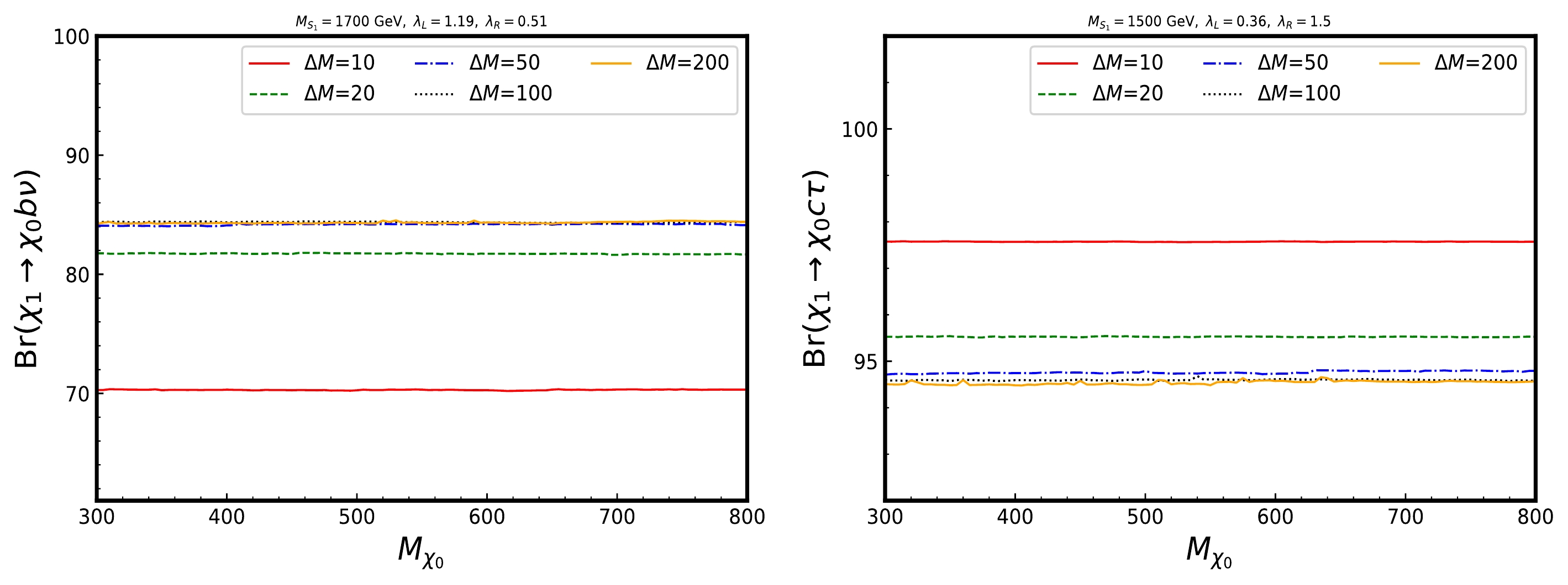

Figure 2.  (color online) The branching ratios (Br$_{\chi_1 \to \chi_0 lq}$) of $\chi_1$ as a function of $M_{\chi_0}$ with the different $\Delta M$.

$ y_{\rm DM} $ appears as a prefactor in amplitude of $\chi_1 \to S_1^* \chi_0 \to \chi_0 lq$, which implies that the branching ratios of $ \chi_1 $ are independent on $y_{\rm DM}$. The results of decay branching ratios are calculated using $ {\mathrm{MadWidth}}$ [105] and $ {\mathrm{FeynRules}}$ [106]. More details for this model (Eq. (1)) are given in Ref. [62].

The cross section of $ \chi_1 \bar{\chi}_1 $ production is larger than that of $ S_1 \bar{S}_1 $ and $ S_1 l $ production for the model of Eq. (1). This process with $ \bar{\chi}_1 $ decay can provide clean collider signatures, including leptons, jets, and missing energy. Therefore, searching for these signatures can further explore the NP. This section details the NLO corrections of $ \chi_1 \bar{\chi}_1 $ production.

The production of a Dirac fermion DM pair $ \chi_1 \bar{\chi}_1 $ at the tree level (partonic) in the lepton colliders is shown in Fig. 3. Only the s-channel $ \gamma/Z $ exchange contributes to the production.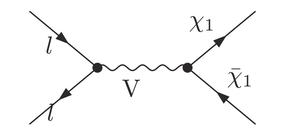

Figure 3.  Tree-level Feynman diagram for DM pair production in the lepton colliders, where $V=\gamma,Z$ and $l =e^\pm, \mu^\pm$.

Now, we use the LQ model as Eq. (1) to explore the production of DM pairs at NLO, as provided by Ref. [62] using the $ {\mathrm{FeynRules}}$($ {\mathrm{FR}}$) [106] model file at LO. However, we rebuild the NLO model file using $ {\mathrm{Lanhep}}$ [107−112] with the on-shell(OS) renormalization scheme. To ensure the accuracy of results, we have validated the results of our model and Ref. [62] at LO, as listed in Table 2. Our results were calculated using $ {\mathrm{FeynArts}}$ [113], $ {\mathrm{FormCalc}}$ [114], and $ {\mathrm{Looptools}}$ [115] ($ {\mathrm{FFL}}$).

Processes	${\mathrm{ FR + Madgraph}}$/pb	$ {\mathrm{Lanhep + FFL}}$/pb
$u \bar{u} \to s_1 \bar{s}_1 $	0.00630(2)	0.00630(1)
$g g \to s_1 \bar{s}_1 $	0.00924(2)	0.00924(1)
$u \bar{u} \to \chi_1 \bar{\chi}_1 $	0.2087(4)	0.2089(1)
$g g \to \chi_1 \bar{\chi}_1 $	1.104(2)	1.103(1)
$s_1 \to \chi_1 \chi_0 $	40.74	40.74

Table 2.  Validating results of our model and Ref. [62] at LO. For the first four processes, we use the physical parameters ($m_{\chi_1}=m_{\chi_0}=600$ MeV, $m_{s_1}=1000$ MeV, and $y_{\rm DM}=1, $$ \lambda_R=\lambda_L=1$), $pp$ collider parameters ($\mu_R=\mu_F=91.188$ MeV and $\sqrt{s}=13$ TeV), and PDF set as $ {\mathrm{NNPDF31-luxQED}}$. For the final process, we consider the mass of $S_1$ as $m_{s_1}=2000$ MeV.

For NLO calculations, two important points need to be addressed, i.e., the cancellation of UV and IR divergences. The UV divergence in virtual corrections can be cancelled by renormalizing the model. The renormalization of theSM is complete [116]; thus, we don't discuss it here. As shown in Fig. 3, the LO process for DM pair production does not include the new couplings. Therefore, it is not necessary to renormalize the new couplings $ \lambda_{R/L} $ or $ y_{DM} $ at NLO. For this study, we need to perform the following renormalization transformation by introducing the corresponding counterterms:

Additionally, for the fields of $ \chi_1,\chi_0 $, and $ S_1 $, we obtain

In Eq. (3), $ \delta Z\chi_{1L/R}, \delta Z \chi_0 $, and $ \delta Z s_1 $ are the counterterms of physical fields. Note that for the renormalization of Majorana Fermion $ \chi_0 $, the antiparticle of $ \chi_0 $is itself; thus, the right-hand part of the counterterm is the conjugate of the left-hand part. Finally, after performing the renormalization transformation for masses and fields (Eqs.(2) and (3)), the UV-finite result in NLO calculations is obtained. Next, we will validate UV divergence in NLO QCD and EW corrections.

Based on the tree-level process shown in Fig. 3, the contribution of the QCD virtual correction is shown in Fig. 4. As $ \chi_1 $ carries the color charge, the virtual gluon exchange appears in between final states and results in triangle contributions. These contributions introduce UV and IR divergences. The heavy $ \chi_1 $value indicates that the IR singularity only exhibits a soft singularity, rather than a collinear singularity. The UV divergences of triangle corrections can be cancelled by combining the counterterms. To separate the divergences induced by loop diagrams, we employ the dimension regularization (DR) and mass regularization (MR) schemes to regularize UV and IR singularities, respectively. By combining the virtual corrections with counter-terms, we obtain a UV-finite result for the NLO QCD corrections as follows: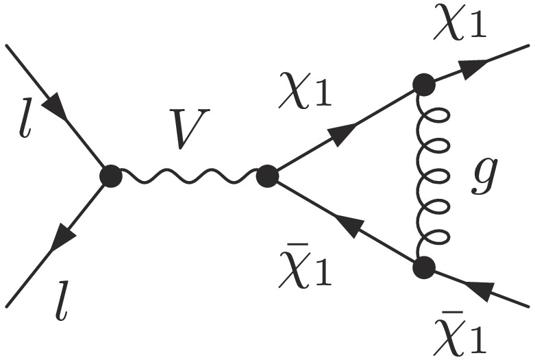

Figure 4.  Feynman diagrams of virtual QCD corrections for $\chi_1 \bar{\chi_1}$ pair production in the lepton colliders.

where $ \sigma_{\text{V}}^{\text{qcd}} $ and $ \sigma_{\text{VC}}^{\text{qcd}} $ denote the cross sections of the virtual correction and counterterm, respectively. λ denotes the mass squared of the gluon in QCD, which is employed to regularize the IR singularities. The λ dependence will be cancelled after considering the real gluon radiation processes. To numerically verify the UV and IR safety of NLO QCD results $ \sigma^{\text{qcd}} = \sigma^{\text{lo}} + \Delta \sigma^{\text{qcd}} $, we use BP0 as the input parameters for the Lagrangian Eq. (1), as listed in Table 3. As indicated in Table 4, we numerically analyze UV divergence (Eq. (4)) by setting different ${1}/{\epsilon_{\text{UV}}}$ values. We consider ${1}/{\epsilon_{\text{UV}}} = 0$ as the baseline result and derive the deviations from this baseline for different values of ${1}/{\epsilon_{\text{UV}}}$. The results in Table 4 indicate that $ \Delta \sigma_{\text{UV-finite}}^{\text{qcd}} $ are independent on ${1}/{\epsilon_{\text{UV}}}$.

	$\mu_R=\mu_F$/GeV	$\sqrt{s}$/GeV	$M_{\chi_0}$/GeV	$M_{\chi_1}$/GeV	$M_{S_1}$/GeV	$\lambda_R$	$\lambda_L$	$y_{DM}$
BP0	91.188	2000	600	600	1000	1	1	1

Table 3.  Input parameters of model Eq. (1), which is used to check the cancellation of UV or IR divergences.

	$\Delta \sigma_{\text{UV-finite}}^{\text{qcd}}$ $\left(\frac{1}{\epsilon_{\text{UV}}} =0\right)$	$\Delta \sigma_{\text{UV-finite}}^{\text{qcd}}$ $\left(\frac{1}{\epsilon_{\text{UV}}} =10^5\right)$	$\Delta \sigma_{\text{UV-finite}}^{\text{qcd}}$ $\left(\frac{1}{\epsilon_{\text{UV}}} =10^{10}\right)$
BP0 /pb	$-7.78\times 10^{-3}$	+ $6\times 10^{-15}$	+ $6\times 10^{-10}$

Table 4.  Analysis of UV divergence cancellation for QCD virtual corrections (Eq. (4)) is summarized, where we conisder photon mass squared as $\lambda = 10^{-3}$. The final two columns show the deviations from the baseline result obtained with $\frac{1}{\epsilon_{\text{UV}}} =0$.

The real gluon radiation corrections for $ \chi_1 \bar{\chi}_1 $ production are depicted in Fig. 5. These contributions only include the soft singularity, which could be cancelled with the virtual QCD corrections. To subtract these IR singularities between virtual and real parts, we use the two cutoff ($ \delta_s, \delta_c $) phase space-slicing method (TCPSS)[94] and the dipole subtraction scheme (DS) [91−93, 117−121]. In this study, we regularize the soft singularities by employing the MR scheme. Next, we briefly describe the two schemes: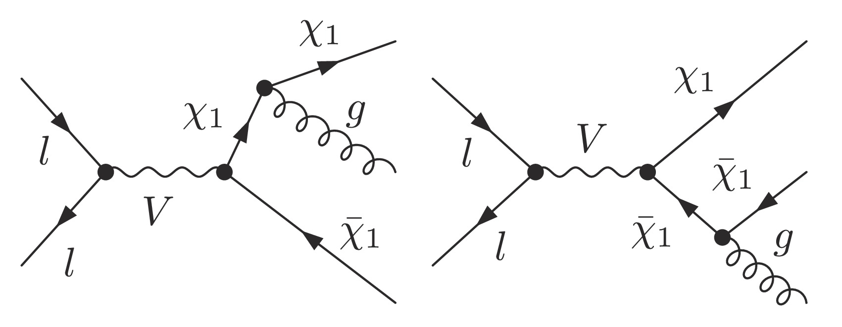

Figure 5.  Feynman diagrams of QCD real radiation processes for $\chi_1 \bar{\chi_1}$ pair production in lepton colliders.

$ \bullet $ TCPSS. For the real QCD corrections in Fig. 5, only a soft singularity exists; thus, we only need one cutoff $ \delta_s $ to separate the phase space of the $ 2 \to3 $ process into hard(H) and soft(S) regions. For the hard region as $ E_g > \left(\delta_s \sqrt{s}\right)/2 $, the integration over the phase space can be directly performed using standard Monte Carlo techniques in four dimensions. In the region of the soft part as $ E_g \leqslant \left(\delta_s \sqrt{s}\right)/2 $, the cross section $ \sigma_{\text{soft}} $ of this region can be defined as a product of LO cross section $ \sigma_0 $ and soft factor $ K_{\text{soft}} $, i.e., $ \sigma_{\text{soft}} = \sigma^{\text{lo}}*K_{\text{soft}} $. The details of $ K_{\text{soft}} $ can be found in Refs. [116, 122]. In this scheme, the full NLO QCD cross section is expressed as

$ \bullet $ DS. Similar to TCPSS (see Eq. (5)), we can derive a full finite NLO QCD cross section in the DS scheme as

We have verified that our results are independent on parameter $ \alpha \in (0,1] $ which was introduced by Refs. [120, 121]. More details on this part are given in [93, 123].

In this study, we consider numerical values to check the dependence of parameters and the cancellation of IR divergences for NLO QCD results. As summarized in Table 5, we perform cross checking for two IR subtraction schemes and further demonstrate that $ \Delta\sigma_{\text{DS(TCPSS)}}^{\text{qcd}} $ is irrelevant with gluon mass in MR scheme.

Schemes	$\lambda = 10^{-3}$			$\lambda = 10^{-7}$
	$\Delta\sigma_{\text{DS}}^{\text{qcd}}$	$\Delta\sigma_{\text{TCPSS}}^{\text{qcd}}$		$\Delta\sigma_{\text{DS}}^{\text{qcd}}$	$\Delta\sigma_{\text{TCPSS}}^{\text{qcd}}$
BP0 /pb	0.87850	0.87869 (0.02%)		0.87851 (${\cal{O}}(10^{-5})$)	0.87871 (0.02%)

Table 5.  Numerical checking of the IR cancellation of gluon radiations for the DS and TCPSS schemes with regard to the MR scheme. The percentages (in the brackets) of the final three results represent the deviation from the first result.

We define the NLO QCD corrections factor as

Compared to the QCD virtual corrections mentioned in Sec. III.C.1, we have more contributions coming from the EW virtual corrections, as shown in Fig. 6. As shown in Fig. 6, the self-energy functions comprise corrections for γ, Z propagator, and mixing between γ and Z. The triangle diagrams originate from $ \gamma,Z $ exchanges between the two particles in the initial or final states and the contributions from W boson and LQ $ S_1 $. The contributions of $ S_1 $ only come from the $ S_1 $-$ \chi_1 $-$ \chi_0 $ vertex, and the corrections for $ llV $ vertex are pure SM contributions. The box diagrams include the contributions of u-$ S_1 $-$ \chi_0 $-$ \bar{S}_1 $ and e-V-$ \chi_1 $-V, which are the UV and IR finite. The UV divergences embedded in EW virtual corrections (self-energy and triangle) can be cancelled by combining EW counterterms. Using Eq. (4), we obtain a UV-finite result after combining the two parts of the EW corrections but for $ \Delta\sigma_{\text{UV-finite}}^{\text{ew}} $. Moreover, the validated results of the UV divergences for the EW corrections are summarized in Table 6.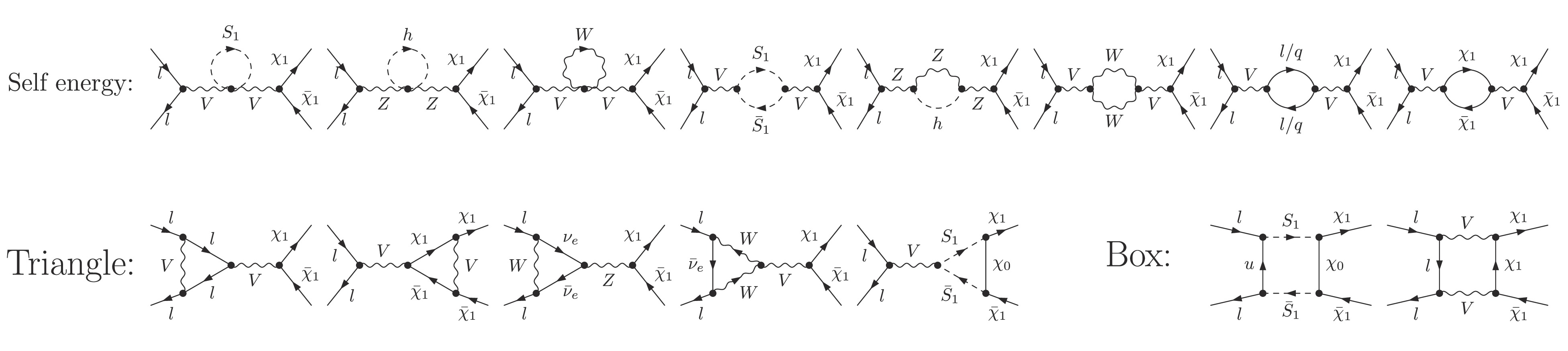

Figure 6.  Feynman diagrams of EW virtual radiation processes for $\chi_1 \bar{\chi_1}$ pair production in the lepton colliders.

	$\Delta\sigma_{\text{UV-finite}}^{\text{ew}}$ $\left(\frac{1}{\epsilon_{\text{UV}}} =0\right)$	$\Delta\sigma_{\text{UV-finite}}^{\text{ew}}$ $\left(\frac{1}{\epsilon_{\text{UV}}} =10^5\right)$	$\Delta\sigma_{\text{UV-finite}}^{\text{ew}}$ $\left(\frac{1}{\epsilon_{\text{UV}}} =10^{10}\right)$
BP0 /fb	$-3.91\times 10^{-3}$	+ $5\times 10^{-15}$	− $2\times 10^{-9}$

Table 6.  Checking the results of UV divergence cancellation according to Table 4 but for EW corrections.

The IR divergences of EW virtual corrections appear only in the virtual photon exchanges, as depicted in the first two subfigures of the triangle diagrams. To eliminate IR singularities in the virtual part, the real photon radiation processes need to be evaluated, as shown in Fig. 7. Compared to the QCD real corrections, we have the extra contributions from the photon radiations off initial leptons, which introduce the additional collinear and soft singularities. Thus, when we deal with the IR singularities by employing the TCPSS schemes, an extra cut $ \delta_c $ is needed to regularize collinear singularity. The hard region was further separated into a hard noncollinear (H$ \bar{\text{C}} $) and hard collinear (HC) regions. The cross section in the HC region can be factorized into a convolution of the LO cross section with a collinear factor in Refs. [124, 125]. Finally, the full finite NLO EW result is expressed as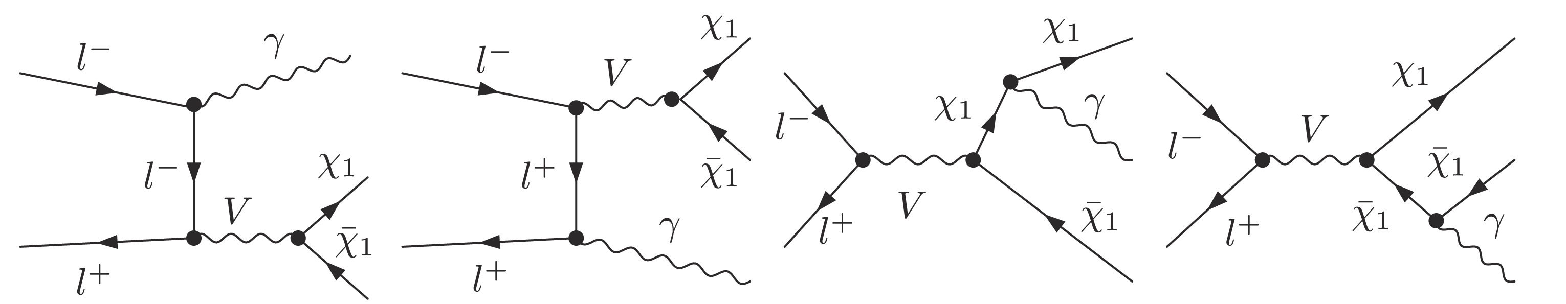

Figure 7.  Feynman diagrams of EW real radiation processes for $l^+ l^- \to \chi_1 \bar{\chi_1}$.

For the DS scheme, the results reveal the same form as Eq. (6), which includes the extra contributions from the initial photon radiation state. More details about the DS scheme for the photon radiation of fermions can be found in Ref. [117]. Similar to Sec. III.C.2, the analysis results of real photon radiation are listed in Table 7.

Schemes	$\lambda = 10^{-3}$			$\lambda = 10^{-7}$
	$\Delta\sigma_{\text{DS}}^{\text{ew}}$	$\Delta\sigma_{\text{TCPSS}}^{\text{ew}}$		$\Delta\sigma_{\text{DS}}^{\text{ew}}$	$\Delta\sigma_{\text{TCPSS}}^{\text{ew}}$
BP0/fb	−0.15716	−0.15766 (0.32%)		−0.15726 (0.06%)	−0.15739 (0.15%)

Table 7.  Numerical checking for the IR cancellation of photon radiations for DS and TCPSS schemes with regard to the MR scheme. The percentages (in the brackets) of the final three results represent the deviation from the first result.

Although higher order initial-state radiation (ISR) contributions are smaller compared to the NLO EW and QCD corrections, we have considered ISR contributions in this study. These corrections can be calculated using the structure–function method [124, 126, 127]. According to the factorization theorem, the leading-logarithmic (LL) initial-state QED correction can be expressed as a convolution of the Born cross section with the structure functions.

The expression of $ \Gamma_{\text{ll}}^{\text{LL}} $ can be found in Refs. [124, 127] up to the $ {\cal{Q}}(\alpha^3_{\text{ew}}) $ order. $ x_{1,2} $ denotes the momentum fractions of the incoming leptons.

To avoid double countering, we must subtract the lowest-order and one-loop contributions.

Here, $ \Gamma_{\text{ll}}^{\text{LL},1} $ denotes the one-loop structure function.

where $ \beta_l = \dfrac{2\alpha_{\text{ew}}}{\pi} \left[\ln \left(\dfrac{Q^2}{m_l^2}\right)-1\right] $.

Previously, we provided a comprehensive description of full NLO EW corrections. However, it is necessary to separate the QED corrections from the EW corrections to calculate the genuine weak corrections. Another reason is that the QED corrections could be quite large and that in leptons initial processes those from the initial state need to be resummed. The QED part exhibits the full real photon radiation (Fig. 7), partial virtual contributions from virtual photon exchange corrections, and the corresponding counterterms. These counterterms contain only the photonic part of the external particle wave function renormalization constants. The remaining contributions of the full NLO EW corrections pertain to the weak corrections as follows:

Following the previous analysis, in this study, we focus on the process $ \chi_1 $-pair production with cascade decaying to $ \chi_0 lq $ as the signal to explore new physical effects in lepton colliders. As $ (\lambda_L)_{33} $ and $ (\lambda_R)_{23} $ are non-zero, we consider the signals of the final $ \chi_0 b \nu_{\tau} $ or $ \chi_0c \tau $ states (Eq. (13)).

which are shown in Fig. 8. In this study, we will consider the full NLO corrections for $ \chi_1 \bar{\chi_1} $ production. The background primarily originates from the processes as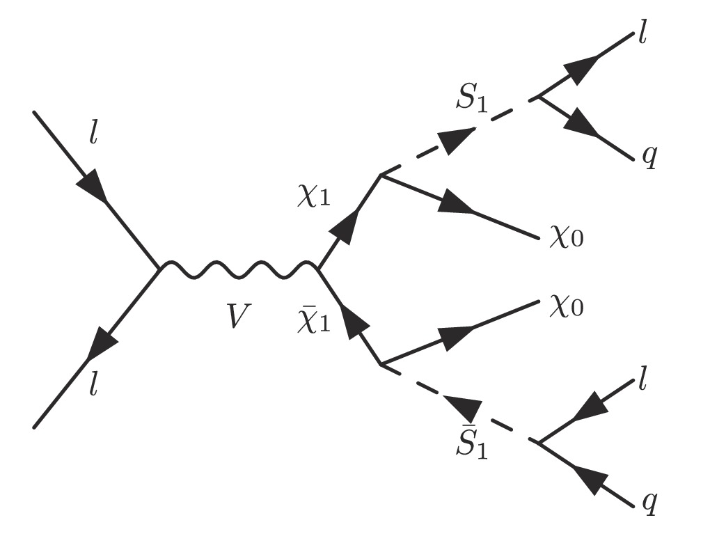

Figure 8.  Signal production chain for the cascade decay of$\chi_1 \bar{\chi}_1$ production in the lepton colliders.

Subdominant backgrounds arise from the production of more neutrino pair, the mis-tagging of b-jets, and other subdominant contributions. The suppressed phase space results in the background from additional neutrino pairs being relatively small. Therefore, this study primarily focuses on the dominant backgrounds of Eq. (14). According to the narrow width approximation (NWA), cross sections for Eq. (13) in the LO and NLO are expressed as

where $ \Delta^{\text{nlo}} $ denotes a factor of NLO corrections as $\Delta^{\text{nlo}} = \dfrac{\sigma_{l^+ l^- \to \chi_1 \bar{\chi_1}}^{\text{nlo}}\ -\ \sigma_{l^+ l^- \to \chi_1 \bar{\chi_1}}^{\text{lo}}}{\sigma_{l^+ l^- \to \chi_1 \bar{\chi_1}}^{\text{lo}}}$.

As shown in Fig. 9, the cross sections for the signal processes (Eq. (13)) as a function of $ M_{\chi_0} $ at $ \sqrt{s} = 3 $ TeV are presented. For the left case, where $ \Delta M = 10 $ GeV, the branching ratio is larger, resulting in a bigger cross section compared to other cases. mM, the behavior of the cross section as a function of $ M_{\chi_0} $ is flatter for the smaller $ \Delta M $ case. By contrast, for the right case, $ \Delta M $ reduces the cross sections of $ \text{Sig}_2 $ in the range of $ M_{\chi_0} \in [300, 1000] $ GeV. The behavior of the cross section as a function of $ M_{\chi_0} $ is similar to the left case. Fig. 10 shows the cross sections of signals and backgrounds as a function of $ \sqrt{s} $. For signal processes, the cross sections increase near the threshold and decrease as $ \sqrt{s} $ moves away from the threshold. By contrast, the cross sections of the background increase with an increase in $ \sqrt{s} $. The results of BP3 and BP4 have overlapped for two cases.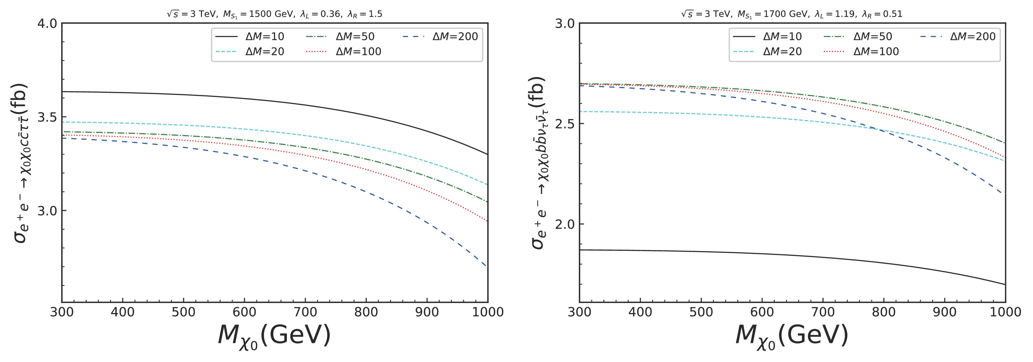

Figure 9.  (color online) Cross sections of signal processes as a function of $M_{\chi_0}$ at $\sqrt{s}$ = 3.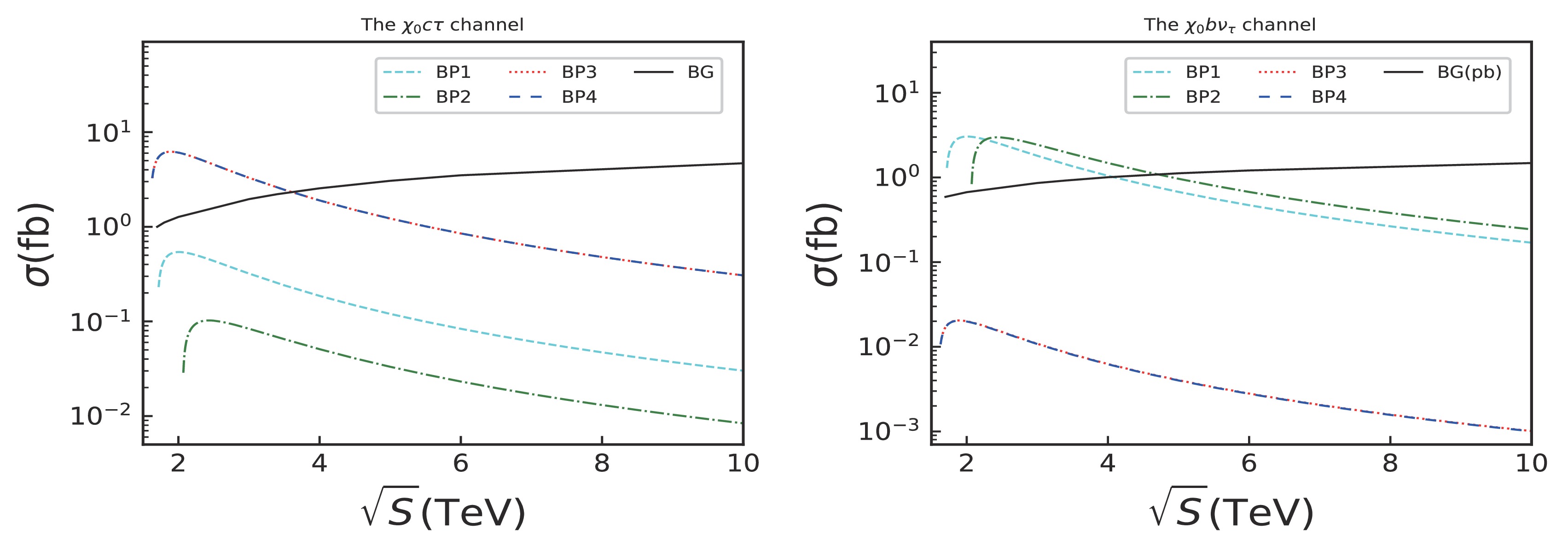

Figure 10.  (color online) Cross sections of signals and backgrounds as a function of $\sqrt{s}$.

Tables 8 and 9 list the numerical results of NLO corrections for $ \chi_1 \bar{\chi}_1 $ production in lepton colliders. We consider $ \sqrt{s} = 2 $ and 3 TeV for the electron–positron collider and $ \sqrt{s} = $ 3, 5 and 10 TeV for the muon collider for expansion. These results indicate that the LO cross section decreases with an increase in $ \sqrt{s} $. The total NLO contributions result in a significant correction to the LO cross sections, increasing with an increase in $ \sqrt{s} $ and exceeding 40% for $ \sqrt{s} = 10 $ TeV. According to the results listed in Table 8, the NLO QCD corrections dominate at 2 TeV, whereas the NLO EW corrections become more significant compared with the QCD corrections at 3 TeV. The QED corrections change from reducing to enhancing the LO cross section for $ \sqrt{s} \in [2, 3] $ TeV. Therefore, calculating NLO corrections is necessary for the analysis of signals and backgrounds.

$\sqrt{s}$	BPs	$\sigma_{\text{LO}}$	$\sigma^{\text{qed}}$ ($\Delta^{\text{qed}}$)	$\sigma^{\text{ew}}$ ($\Delta^{\text{ew}}$)	$\sigma^{\text{qcd}}$($\Delta^{\text{qcd}}$)	$\sigma^{\text{nlo}}$ ($\Delta^{\text{nlo}}$)
2 TeV	BP1	6.15	5.33(−13.3%)	6.62(7.71%)	7.92(28.8%)	8.39(36.5%)
	BP3	6.79	6.20(−8.64%)	7.46(9.92%)	8.33(22.6%)	9.00(32.5%)
	BP4	6.79	6.20(−8.64%)	7.59(11.8%)	8.33(22.6%)	9.13(34.4%)
3 TeV	BP1	3.64	3.85(5.69%)	4.58(25.7%)	4.00(9.80%)	4.93(35.5%)
	BP2	3.42	3.39(−0.87%)	4.07(18.9%)	3.92(14.5%)	4.57(33.4%)
	BP3	3.68	3.95(7.36%)	4.69(27.5%)	4.01(8.86%)	5.02(36.4%)
	BP4	3.68	3.95(7.36%)	4.69(27.4%)	4.01(8.86%)	5.02(36.2%)

Table 8.  NLO corrections of cross sections for $\chi_1\bar{\chi}_1$ production in the electron collider are presented. The unit of cross section is fb.

$\sqrt{s}$	BPs	$\sigma_{\text{LO}}$	$\sigma^{\text{qed}}$ ($\Delta^{\text{qed}}$)	$\sigma^{\text{ew}}$ ($\Delta^{\text{ew}}$)	$\sigma^{\text{qcd}}$($\Delta^{\text{qcd}}$)	$\sigma^{\text{nlo}}$ ($\Delta^{\text{nlo}}$)
3 TeV	BP1	3.64	3.78(3.94%)	4.54(24.6%)	4.00(9.80%)	4.90(34.4%)
	BP2	3.42	3.41(−0.30%)	4.11(20.1%)	3.92(14.5%)	4.61(34.6%)
	BP3	3.68	3.87(5.02%)	4.63(25.8%)	4.01(8.86%)	4.96(34.7%)
	BP4	3.68	3.87(5.02%)	4.63(25.7%)	4.01(8.86%)	4.95(34.5%)
5 TeV	BP1	1.36	1.53(11.8%)	1.81(32.7%)	1.44(5.43%)	1.88(38.1%)
	BP2	1.36	1.48(9.30%)	1.76(30.1%)	1.44(6.40%)	1.85(36.5%)
	BP3	1.37	1.54(12.6%)	1.83(34.2%)	1.44(5.21%)	1.90(39.4%)
	BP4	1.37	1.54(12.6%)	1.82(33.5%)	1.44(5.22%)	1.89(38.7%)
10 TeV	BP1	0.34	0.415(21.0%)	0.49(42.2%)	0.36(4.15%)	0.50(46.4%)
	BP2	0.34	0.407(18.8%)	0.48(39.0%)	0.36(4.32%)	0.49(43.3%)
	BP3	0.34	0.417(21.7%)	0.46(35.1%)	0.36(4.10%)	0.48(39.2%)
	BP4	0.34	0.417(21.7%)	0.49(42.8%)	0.36(4.10%)	0.50(46.9%)

Table 9.  NLO corrections of cross sections for $\chi_1\bar{\chi}_1$ production in the muon collider are presented. The unit for cross section is fb.

To better illustrate the behaviors of NLO contributions, Fig. 11 shows the correction factors as a function of $ \sqrt{s} $ in the muon colliders over the range of $ \sqrt{s} \in [1.6, 10] $ TeV. The cross sections increase near 2 TeV and then decrease continuously with an increase in$ \sqrt{s} $ values. The results for BP1 and BP4 exhibit similar behavior throughout the range of $ \sqrt{s} \leqslant 10 $ TeV. From Fig. 11, we observe that the QCD corrections are positive and quite large near the threshold region ($ \sqrt{s} \sim 2 M_{\chi_1} $), where soft-gluon exchange in the $ \chi_1 \bar{\chi}_1 $ system leads to a Coulomb-like singularity. This singularity could be diluted by the larger phase space if $ \sqrt{s} $ is away from the threshold, the development of singularity is enhanced at a low relative velocity of $ \chi_1 $. The photonic corrections (QED) are large and negative when $ \sqrt{s} $ is not too far from the threshold. This occurs because as $ \sqrt{s} $ approaches the threshold, large virtual photonic corrections arise which are not canceled by the corresponding real radiation owing to the decreasing phase-space region for real photon emission. Therefore, the resummation of photonic corrections is essential, with part of this contribution being accounted for in higher order ISR corrections. Moreover, cancellation can be observed between ISR and QED corrections near the threshold region. After subtracting the QED corrections from the EW corrections, the weak corrections become stable across the full range of $ \sqrt{s} $. As $ \sqrt{s} $ increases, the QED corrections transition from reducing to enhancing the LO cross sections. Combining the results of Table 8, it is evident that the EW corrections are larger than the QCD corrections and more pronounced for$ \sqrt{s} > $ 2.1 TeV.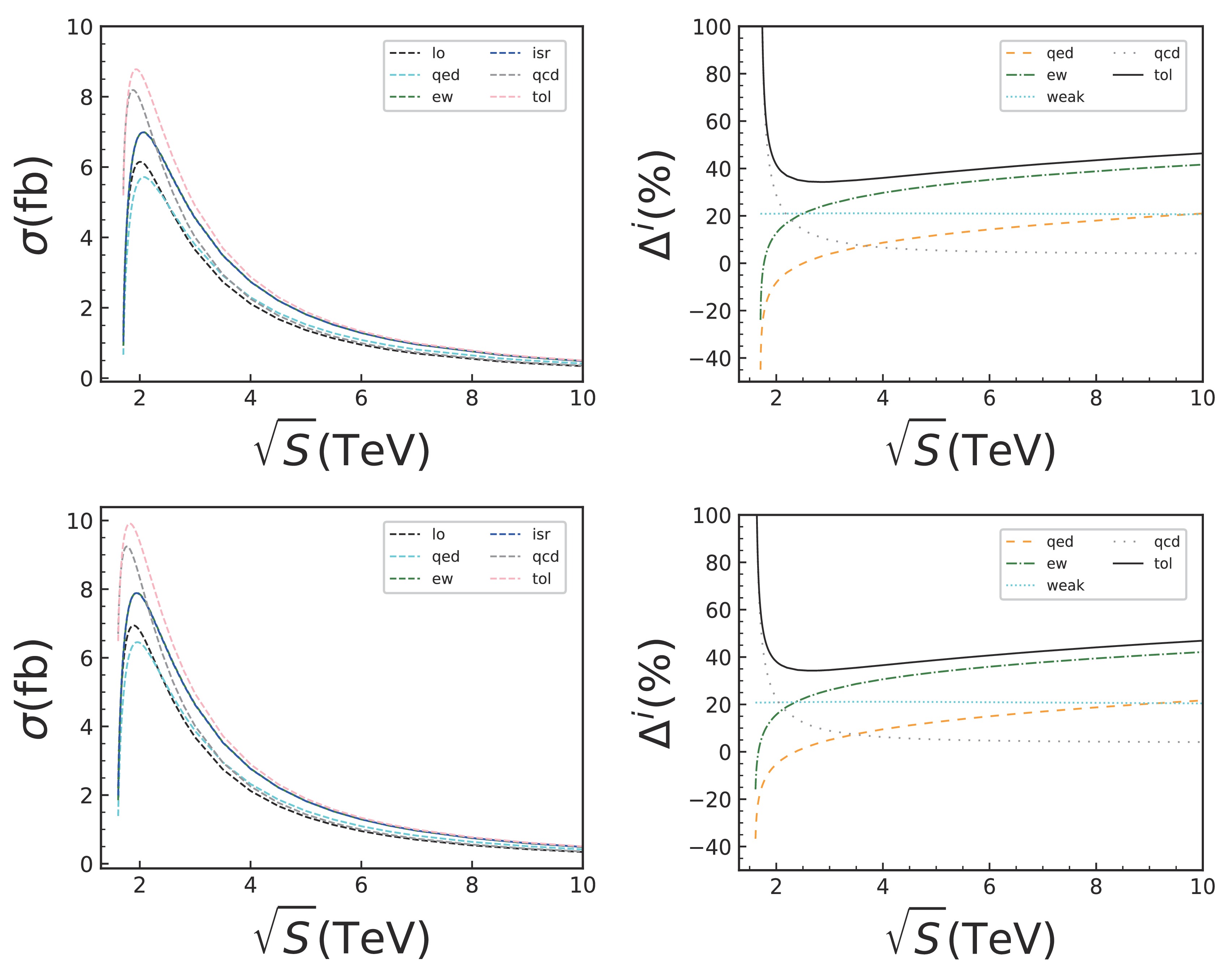

Figure 11.  (color online) NLO correction results as a function of$\sqrt{s}$ for BP1 and BP4 in the muon collider are shown in upper and lower panels, respectively.

Next, we present the analysis results of the signal processes (Eqs. (13) and (14)) at the parton level. The events for these processes are generated using $ {\mathrm{MadGraph}}$ [128]. The signal significance is defined as

where $ {\cal{N}}_{S/B} $ denotes the events of signal and background and $ \epsilon\ {\rm{is}} $ the systematic uncertainty in background estimation. $ {\cal{S}} $ denotes the signal significance with the kinematic cuts. From Table 1, the $ \chi_0 b \nu_{\tau} $ and $ \chi_0 c \tau $ channels dominate the first two and the final two BPs, respectively. Therefore, we will analyze the process $ \text{Sig}_2 $ for BP1 and BP2, and $ \text{Sig}_1 $ for BP3 and BP4, respectively.

This section presents the main results for the $ \text{Sig}_1 $ process, as shown in Table 10. From Table 10, the cross sections of signal are decrease with the increasing of $ \sqrt{s} $, while the cross sections of background are increase. The values of both are about of the same order, except for the $ \sqrt{s} = 10 $ TeV case at muon collider. Secondly, without any kinematic cuts, the significances for the $ \text{Sig}_1 $ process are also described in Table 10 with $ {\cal{L}} = 1\text{ fb}^{-1} $. The values of signal significance for the $ \text{Sig}_1 $ process can reach 2σ sensitivity for $ \sqrt{s} = 2 $ TeV. Moreover, $ S^{lo} $ approaches 2σ sensitivity for $ \sqrt{s} = 3 $ TeV and are approximately $ {\cal{O}}(10^{-1}) $ for $ \sqrt{s} = 5 $ and 10 TeV. To improve the efficiency of signal identification at higher $ \sqrt{s} $, we can choose a series of kinematic cuts based on the characteristics related to our signal and background.

$\sqrt{s}$	BPs	$\sigma_{\text{S}}$/pb	$\sigma_{\text{B}}$/pb	${\cal{S}}^{\text{lo}}$	${\cal{S}}$	${\cal{S}}(\epsilon$=1%)
2 TeV	BP3	6.07	1.27	2.24	x	x
	BP4	6.08	1.27	2.24	x	x
3 TeV	BP3	3.29	1.96	1.44	1.65	1.65
	BP4	3.29	1.96	1.44	1.41	1.41
3 TeV	BP3	3.29	1.96	1.44	1.65	1.65
	BP4	3.29	1.96	1.44	1.41	1.41
5 TeV	BP3	1.23	3.06	0.59	1.02	1.02
	BP4	1.23	3.06	0.59	0.86	0.86
10 TeV	BP3	0.30	4.69	0.14	0.44	0.44
	BP4	0.30	4.69	0.14	0.50	0.50

Table 10.  Results of cross sections for the signal and background, as well as the signal significance for $ {\rm{Sig}}_1$, are presented. "x" means that the kinematic cuts give the negative contribution for significance. The upper and lower panels are the results of electron–positron and muon colliders with ${\cal{L}}=1\text{ fb}^{-1}$, respectively.

For higher $ \sqrt{s} $ cases in the muon collider, the $p_T^{{\rm jet}}$ and $ \not{E}_T $ distributions of the signal are almost completely covered by the background results. The cuts on transverse momentum for these kinematic variables do not offer high efficiency for distinguishing the signal from the background and may even result in negative efficiencies; we give a symbol “x” for this in Table 10. Therefore, these kinematic variables are not considered to distinguish the signal and background. As shown in Fig. 12, the invariant mass distributions of light jet, τ leptons, and missing energy are shown. For $ \sqrt{s} = 2 $ TeV, the distributions of BP4 with small mass splitting between $ \chi_1 $ and $ \chi_0 $ are sharper compared with those of BP3, and the distributions of $M_{{inv}}^{{\rm miss}}$ are clearer. To specify this behavior, Fig. 13 shows various kinematic distributions for $ \Delta M \in [50,400] $ GeV. Fig. 13 shows that as $ \Delta M $ increases, the kinematic distributions become gradually flatter and the peak locations shift away. Combining the results from Fig. 12, the efficiency for distinguishing the signal from the background decreases as $ \Delta M $ increases. There is a clear peak around $ \sqrt{s} \approx M_Z $ for the distribution of $M_{inv}^{{\rm jet}}$ and an extra clear peak around $ \sqrt{s} \approx M_h $ for the distribution of $ M_{inv}^{\tau} $ in the $ \text{Sig}_1 $ process. Comparing the upper and lower panels of Fig. 12, the distributions of $M_{{inv}}^{{\rm jet}(\tau)}$ are wider at $ \sqrt{s} = 3 $ TeV. Thus, the cuts on kinematic variables $ M_{{inv}} $ could be potential candidates for improving the efficiencies of signal. The behaviors of kinematic distributions in the muon collider are similar to the $ e^+ e^- $ case; thus, we will not show it here.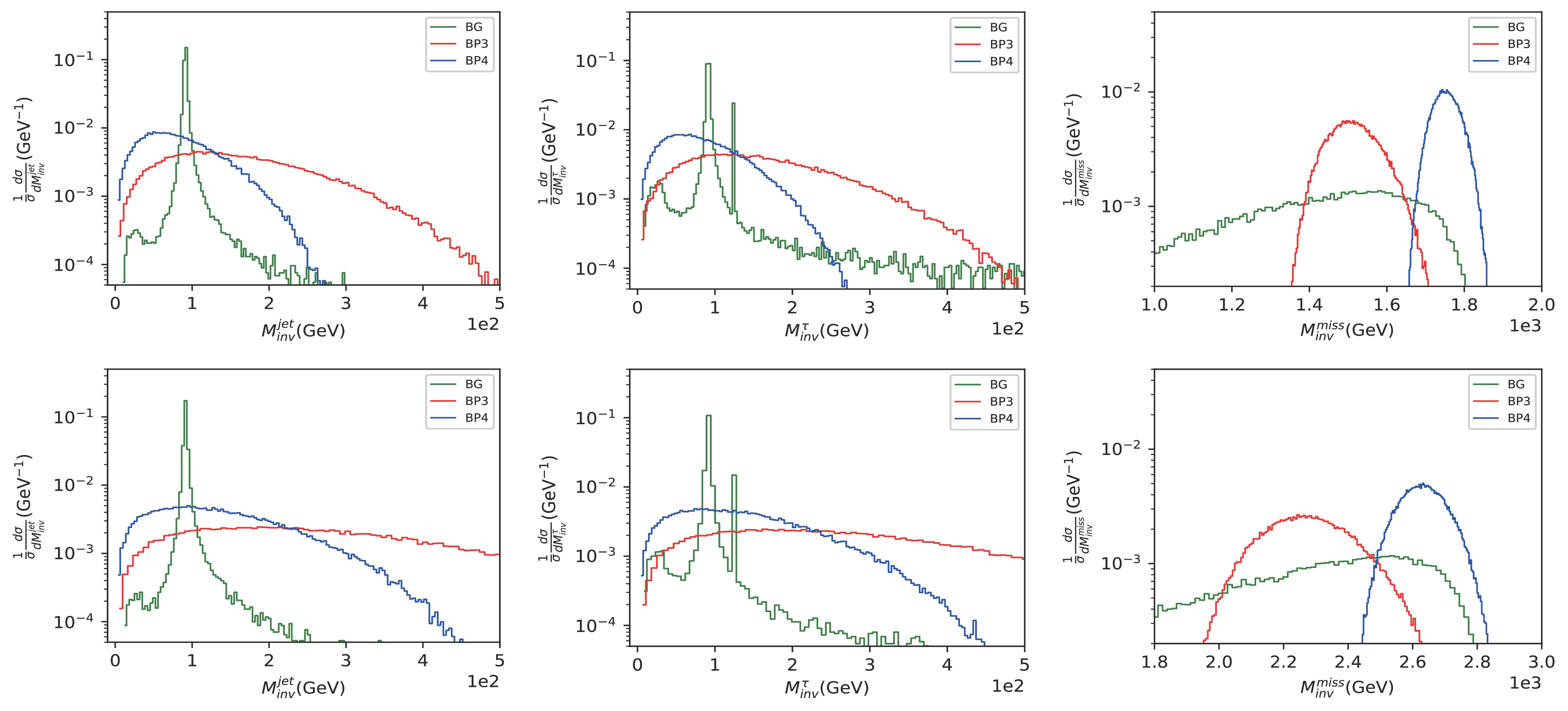

Figure 12.  (color online) Invariant mass distributions for the $ {\rm{Sig}}_1$ process in the electron colliders. The upper and lower panels depict the results of $\sqrt{s}=2$ TeV and $\sqrt{s}=3$ TeV, respectively.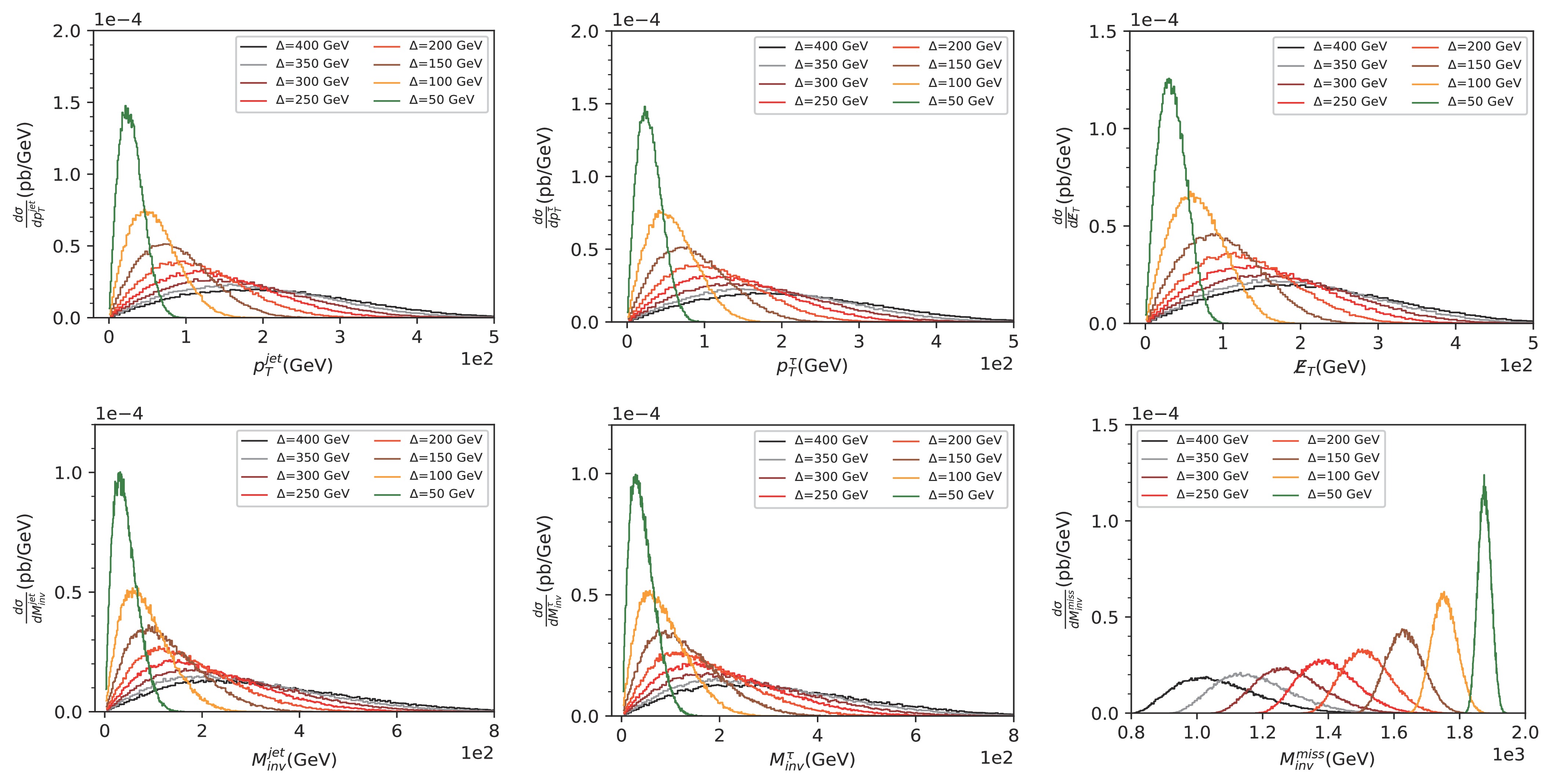

Figure 13.  (color online) Kinematic distributions in the $ {\rm{Sig}}_1$ process for mass splitting $\Delta M$ are shown.

Table 11 indicates that according to the distributions results shown in Fig. 12, the cuts on kinematic variables help improve the efficiency of signal identification. Fig. 12 shows that the overlap between the signal and background regions for the $M_{inv}^{\rm miss}$ distribution becomes progressively larger as $ \sqrt{s} $ increases. The cut on $M_{inv}^{\rm jet}$ is insufficient for a higher number of $ \sqrt{s} $ cases. Thus, the cuts on the distributions of $M_{inv}^{\rm jet}$ and $ M_{inv}^{\tau} $ are the primary candidates for the $ \chi_0 c \tau $ channel. In final two columns of Table 10, the significance values after implementing the kinematic cuts are provided. For $ \sqrt{s} = 2 $ TeV, we do not consider any cuts to reduce the events of the signal and background. The improvement in the cuts are mainly observed for a higher number of$ \sqrt{s} $ cases. The background events could be reduced by applying the cut $M_{inv}^{\rm jet} > 100$ GeV, even without any cut on $ M_{inv}^{\tau} $, for $ \sqrt{s} = 3 $ TeV. However, for $ \sqrt{s} \geqslant 5 $ TeV, the cut $M_{inv}^{\rm jet} > 100$ GeV alone is inadequate, and the cut $ M_{inv}^{\tau} > 130 $ GeV is a candidate to further reduce the background. After considering the kinematic cuts in Table 11, the final two columns of Table 10 list the results of signal significance $ {\cal{S}} $. The cross section of the$ \chi_0 c \tau $ channel decreases with an increase in $ \sqrt{s} $, while the efficiency of cuts improving the signal significance increases. The final column of Table 10 indicates that systematic uncertainty (1%) does not affect the significance. Therefore, for a higher number of $ \sqrt{s} $ cases, we can expect that the signal significance could be further improved by considering the NLO corrections.

$\sqrt{s}$	Cuts
3 TeV	$M_{inv}^{\rm jet}$ > 100 GeV
$> 5$ TeV	$M_{inv}^{\rm jet}$ > 100 GeV, $M_{inv}^{\tau}$ > 130 GeV

Table 11.  Cuts considered to improve the efficiency of signal identification for the $ {\rm{Sig}}_1$ process are shown.

Based on the aforementioned results, we expect that the signal significance can be further improved. The kinematic cuts strongly reduce the background events, with some cuts making the background negligible. Thus, the signal significance can be further enhanced by applying the NLO correction factors (Tables 8 and 9) to the signal processes. Table 12, we show the cross sections and signal significances for the $ \chi_0 c \tau $ channel, incorporating the NLO correction factors. The factor $ \Delta_{\cal{S}} = ({\cal{S}}^{\text{i}} - {\cal{S}}) / {\cal{S}} $ quantifies the contribution of the NLO corrections relative to the LO. The final column indicates that as $ \sqrt{s} $ increases, the enhancement from the NLO corrections becomes more significant. As discussed in Sec. V. A, the EW corrections gradually dominate, whereas the QCD corrections become smaller for higher $ \sqrt{s} $. At $ \sqrt{s} = 10 $ TeV, the NLO corrections improve the LO significance by approximately 24% and 22% for BP3 and BP4, respectively. Even at $ \sqrt{s} = 2 $ TeV, NLO corrections enhance the significance by approximately 18% for both BPs.

$\sqrt{s}$	BPs	$\sigma_{\text{S} }^{\text{nlo} }/{\text{fb} }$	${\cal{S}}^{\text{qed}}(\Delta_{{\cal{S}}})$	${\cal{S}}^{\text{ew}}(\Delta_{{\cal{S}}})$	${\cal{S}}^{\text{qcd}}(\Delta_{{\cal{S}}})$	${\cal{S}}^{\text{nlo}}(\Delta_{{\cal{S}}})$
2 TeV	BP3	8.05	2.13(−5.17%)	2.37(5.67%)	2.52(12.5%)	2.64(17.6%)
	BP4	8.17	2.13(−5.17%)	2.39(6.17%)	2.52(12.5%)	2.66(18.6%)
3 TeV	BP3	4.49	1.71(3.80%)	1.87(13.5%)	1.72(4.55%)	1.94(17.6%)
	BP4	4.48	1.47(3.86%)	1.61(13.7%)	1.48(4.62%)	1.66(17.8%)
3 TeV	BP3	4.43	1.69(2.59%)	1.86(12.8%)	1.72(4.55%)	1.93(16.8%)
	BP4	4.43	1.45(2.63%)	1.59(12.9%)	1.48(4.62%)	1.65(17.0%)
5 TeV	BP3	1.71	1.08(6.19%)	1.18(16.0%)	1.04(2.61%)	1.21(18.3%)
	BP4	1.70	0.91(6.22%)	0.99(15.8%)	0.88(2.62%)	1.01(18.1%)
10 TeV	BP3	0.42	0.58(13.9%)	0.62(21.8%)	0.54(2.73%)	0.63(24.2%)
	BP4	0.45	0.55(10.9%)	0.60(20.5%)	0.51(2.14%)	0.61(22.3%)

Table 12.  Results of the cross sections and the signal significance${\cal{S}}^i$ at NLO for $ {\rm{Sig}}_1$ with $\epsilon=0$ are shown. The upper and lower panels depict the results of electron and muon colliders, respectively.

The left and right panels of Fig. 14 show the contour plots of the expected $ 2\sigma $ sensitivity for the LO and NLO, respectively. For the LO and NLO, except for the $ \sqrt{s} = 2 $ TeV case, the signal significance is almost independent on $ M_{\chi_0} $. The NLO corrections could reduce the required luminosity across the $ M_{\chi_0} $ range, which is approximately 10 fb $ ^{-1} $ at a $ \sqrt{s} = 10 $ TeV muon collider. In the high $ M_{\chi_0} $ region for $ \sqrt{s} = 2 $ TeV, the cross section decreases with an increase in $ M_{\chi_0} $, as shown in Fig. 9. Thus, the required luminosity increases as $ 2M_{\chi_0} $ approaches the threshold.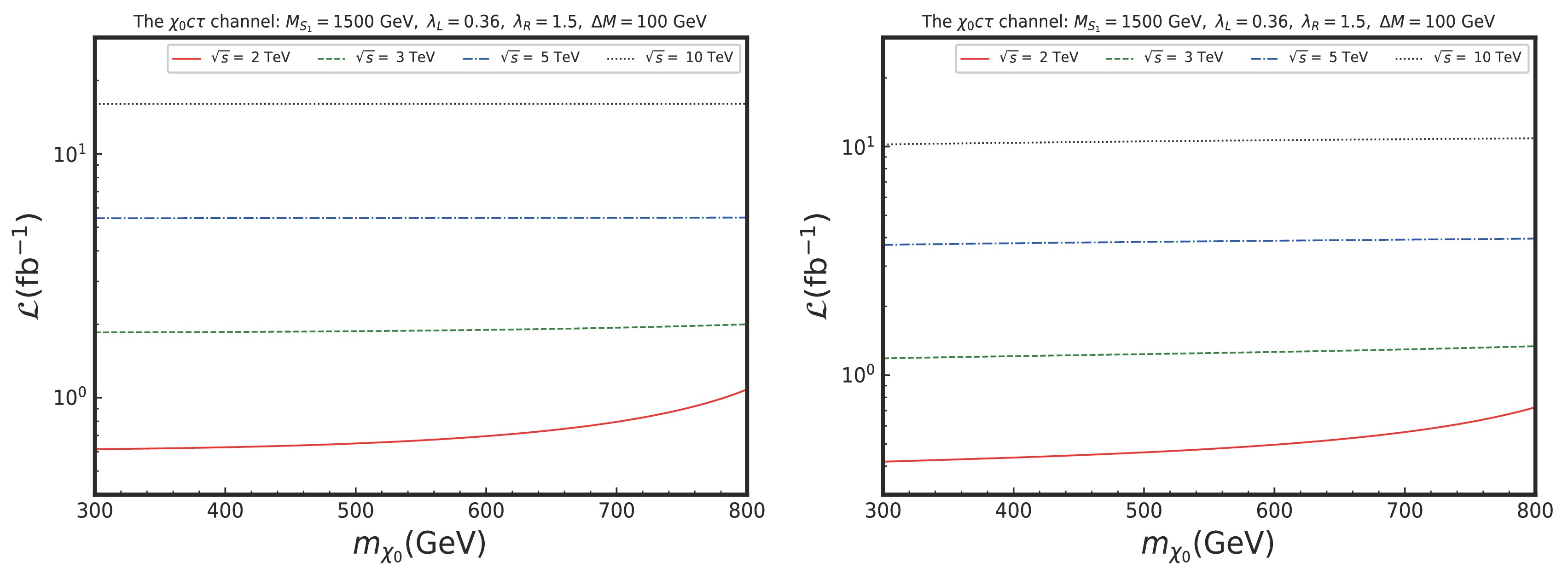

Figure 14.  (color online) Contour plots in luminosity: $M_{\chi_0}$ planes for the LO and NLO are shown in the left and right panels, respectively.

The results of the cross sections for the $ \text{Sig}_2 $ process in the lepton colliders are listed in Table 13. Similar to the $ \text{Sig}_1 $ case, as $ \sqrt{s} $ increases, the cross sections of the signal decrease, while the background increases. The background cross sections are roughly three orders of magnitude larger than the signal, with a greater difference for $ \sqrt{s} = 10 $ TeV in the muon colliders. Without any kinematic cuts, the significance values of the $ \text{Sig}_2 $ process are listed in Table 13 with $ {\cal{L}} = 1\text{ fb}^{-1} $. The values of $ {\cal{S}}^{\text{lo}} $ decrease from the order of $ {\cal{O}}(10^{-1}) $ to $ {\cal{O}}(10^{-3}) $ as $ \sqrt{s} $ increases. To improve the efficiency of signal identification, we can choose a series of kinematic cuts based on the characteristics related to our signal and background. Fig. 15 shows the results of kinematic distributions for $ \text{Sig}_2 $. The upper panel of Fig. 15 shows that BP2 is close for $ \sqrt{s} = 2 $ TeV; all the kinematic distributions exhibit the difference between BP1 and the background. The peaks of $M_{inv}^{\rm miss}$ for BP1 and background are even farther apart from each other. For $ \sqrt{s} \geqslant 3 $ TeV, in the lower panel of Fig. 15, the results indicate that BP1 has a sharper peak compared with BP2 in all kinematic distributions. This behavior arises from mass splitting between $ \chi_1 $ and $ \chi_0 $, which has been described in the previous sections. The distributions of $ p_T^{\text{jet}} $ and $ \not {E}_T $ exhibit similar behaviors, with peaks located in the region of small values. The peak of BP1 is positioned farther from the background peak compared with that of BP2, while BP2 exhibits a wider overlap with the background. The efficiency of signal identification can be improved by implementing cuts on $ p_T^{\text{jet}} $ or $ \not{E}_T $, with BP1 being more effective than BP2. For the distributions of $M_{inv}^{\rm jet}$, the background exhibits two peaks around the masses of SM Z and Higgs, respectively. These peaks are clearly distinct from the peak of BP1, indicating a cut to distinguish the signal and background. For the distributions of $M_{inv}^{\rm miss}$, a considerable distinction can be observed between the signal (small mass splitting) and background in the region of large values (for BP2, there is an additional overlap area compared to BP1). Similar to the $ \text{Sig}_1 $ process, the kinematic distributions in the muon collider are comparable to the $ e^+ e^- $ collider.

$\sqrt{s}$	BPs	$\sigma_{\text{S}}$/fb	$\sigma_{\text{B}}$/pb	${\cal{S}}^{\text{lo}}$	${\cal{S}}$	${\cal{S}}(\epsilon$=1%)
2 TeV	BP1	3.04	0.67	0.118	1.67	1.67
3 TeV	BP1	1.80	0.86	0.061	0.82	0.82
	BP2	2.43	0.86	0.083	0.55	0.55
3 TeV	BP1	1.80	0.86	0.061	0.82	0.82
	BP2	2.43	0.86	0.083	0.55	0.55
5 TeV	BP1	0.67	1.12	0.020	0.27	0.27
	BP2	0.97	1.12	0.029	0.29	0.29
10 TeV	BP1	0.17	1.48	0.004	0.060	0.060
	BP2	0.24	1.48	0.006	0.065	0.065

Table 13.  Results of the cross sections of the signal and background, as well as signal significance for ${\rm{Sig}}_2$, are presented. The upper and lower panels depict the results of electron–positron and muon colliders with${\cal{L}}=1\text{ fb}^{-1}$, respectively.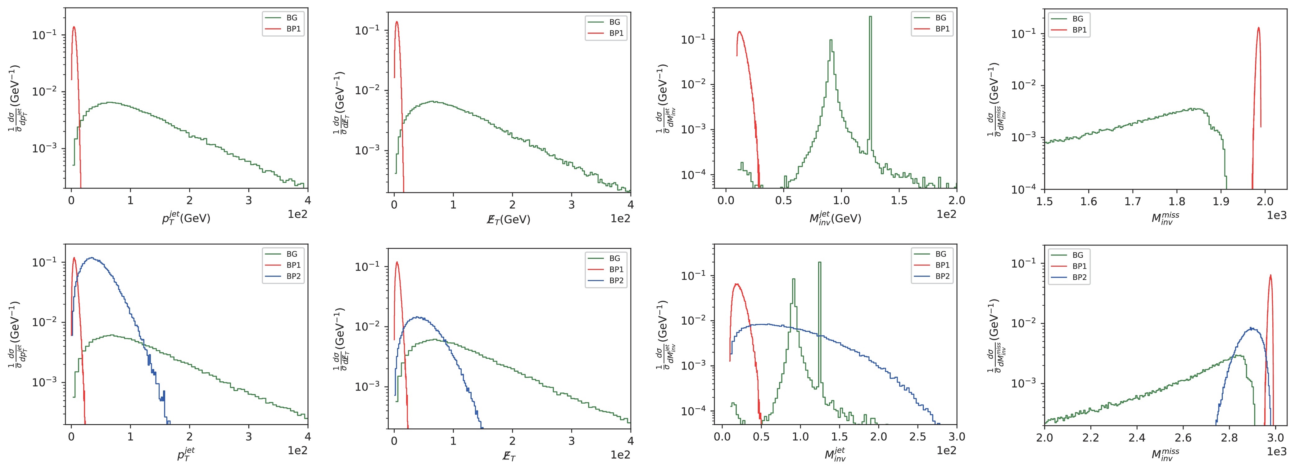

Figure 15.  (color online) Kinematic distributions of the ${\rm{Sig}}_2$ process in the electron colliders; the cross sections have been normalized. The upper and lower panels represent the results of $\sqrt{s}=2$ and $\sqrt{s}=3$ TeV, respectively.

Table 14 lists the kinematic cuts, chosen to improve the efficiency of signal identification for the $ \text{Sig}_2 $ process. For $ \sqrt{s} \leqslant 5 $ TeV, we can reduce the background by restricting $M_{inv}^{\rm miss}$ to larger values, specifically for BP1 with a small value of $ \Delta M $. BP2 with larger mass splitting exhibits a more flattened distribution, and the background is mainly concentrated around the peaks of $ M_Z $ and $ M_h $ in the $M_{inv}^{\rm jet}$ distribution. Thus, the cuts $M_{inv}^{\rm jet} < 80$ GeV and $M_{inv}^{\rm jet} > 130$ GeV vetoing the peaks of $M_{inv}^{\rm jet}$ can be used to further reduce the background events. For $ \sqrt{s} = 10 $ TeV, to minimize the events of the background, we apply different $M_{inv}^{\rm miss}$ cut schemes for BP1 and BP2, with the cuts in the brackets used for BP2. The larger value of $ \Delta M $ for BP2 results in a flatter distribution of $M_{inv}^{\rm miss}$, with the peak shifted further to the left. Thus, we need a smaller cut on $M_{inv}^{\rm miss}$ for BP2 at $ \sqrt{s} = 10 $ TeV as in bracket of Table 14. In summary, for a higher number of $ \sqrt{s} $ cases, we need to restrict $M_{inv}^{\rm miss}$ to a larger range and veto the peaks of $M_{inv}^{\rm jet}$. After applying the kinematic cuts listed in Table 14, the final signal significance results are presented in the last two columns of Table 13. The largest efficiency improvement in significance is more than an order of magnitude, while even the lowest efficiencies improve by more than half an order of magnitude. Although the background cross section is approximately three orders of magnitude larger than the signal, the kinematic cuts considerably reduce the number of background events, ensuring that systematic uncertainties (1%) do not affect the significance. Hence, DM signals can be explored in CLIC or muon colliders by increasing luminosity in the final $ j_b j_b $ + ME states in the future.

$\sqrt{s}$	Cuts
2 TeV	$M_{inv}^{\rm miss} > 1900$ GeV
3 TeV	$M_{inv}^{\rm miss} > 2800$ GeV, $M_{inv}^{\rm jet} < 80$ GeV and $M_{inv}^{\rm jet} > 130$ TeV
5 TeV	$M_{inv}^{\rm miss} > 4600$ GeV, $M_{inv}^{\rm jet} < 80$ GeV and $M_{inv}^{\rm jet} > 130$ TeV
10 TeV	$M_{inv}^{\rm miss} > 9800 \;{\text{GeV} }$ $\left(M_{inv}^{\rm miss} > 9250\ \text{GeV}\right)$, $M_{inv}^{\rm jet} < 80 \;{\text{GeV} }$ and $M_{inv}^{\rm jet} > 130 \;{\text{TeV} }$

Table 14.  Cuts considered to improve the efficiency of signal identification for the ${\rm{Sig}}_2$ process.

Similar to the $ \chi_0 c \tau $ channel, Table 15 and Fig. 16 present the results of the cross sections and the signal significance at NLO for the $ \text{Sig}_2 $ process. The behavior of the results for the $ \chi_0 b \nu_{\tau} $ channel is similar to the $ \chi_0 c \tau $ channel. However, the NLO corrections enhance the signal significance more in the $ \chi_0 b \nu_{\tau} $ channel compared to the $ \chi_0 c \tau $ channel, with an improvement of over 40% at $ \sqrt{s} = 10 $ TeV. As shown in Fig. 16, the NLO correction factor can further reduce the required luminosity to achieve the expected $ 2\sigma $ sensitivity.

$\sqrt{s}$	BPs	$\sigma_{\text{S} }^{\text{nlo} }/{\text{fb} }$	${\cal{S}}^{\text{qed}}(\Delta_{{\cal{S}}})$	${\cal{S}}^{\text{ew}}(\Delta_{{\cal{S}}})$	${\cal{S}}^{\text{qcd}}(\Delta_{{\cal{S}}})$	${\cal{S}}^{\text{nlo}}(\Delta_{{\cal{S}}})$
2 TeV	BP1	4.15	1.54(−7.48%)	1.74(4.10%)	1.91(14.6%)	1.97(18.2%)
3 TeV	BP1	2.44	0.86(4.58%)	0.99(20.0%)	0.89(7.83%)	1.05(27.3%)
	BP2	3.24	0.59(−0.77%)	0.69(15.8%)	0.67(12.2%)	0.76(27.4%)
3 TeV	BP1	2.42	0.85(3.14%)	0.98(19.2%)	0.89(7.83%)	1.04(26.4%)
	BP2	3.28	0.59(−0.26%)	0.69(16.7%)	0.67(12.2%)	0.76(28.3%)
5 TeV	BP1	0.93	0.30(11.1%)	0.35(30.4%)	0.28(5.10%)	0.36(35.4%)
	BP2	1.32	0.28(8.63%)	0.32(27.6%)	0.27(5.95%)	0.34(33.3%)
10 TeV	BP1	0.25	0.073(20.6%)	0.085(41.2%)	0.063(4.12%)	0.088(45.2%)
	BP2	0.35	0.077(18.8%)	0.090(38.4%)	0.067(4.25%)	0.092(42.6%)

Table 15.  Results of the cross sections and the signal significance ${\cal{S}}^i$ at NLO for ${\rm{Sig}}_2$ with $\epsilon=0$ are shown. The upper and lower panels represent the results of the electron and muon colliders, respectively.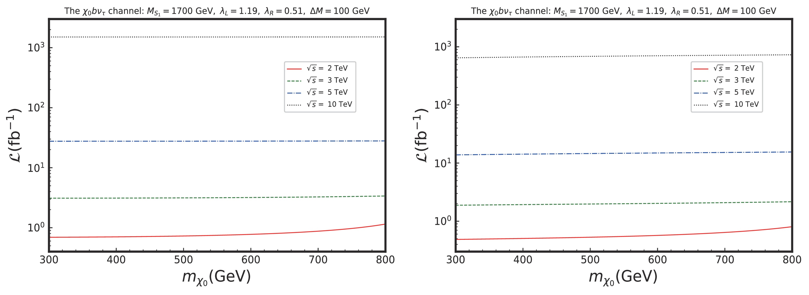

Figure 16.  (color online) Contour plots in luminosity: $M_{\chi_0}$ planes for the LO and NLO are shown in the left and right panels, respectively.

The leptoquark plus dark matter model, proposed by Ref. [62], exhibits a rich content of phenomenology. In this study, full NLO corrections, including QCD, EW, and ISR for heavy DM pair production, are calculated in electron–positron and muon colliders. For real radiation correction, we detail the regularization of IR singularities using the mass regularization scheme. Except for the NLO QCD and EW corrections, for lepton initial-state processes, we have considered ISR corrections. Moreover, we demonstrate that the EW corrections become more significant at higher collision energies, eventually dominating the NLO corrections over the QCD corrections. The heavy DM cascade decaying to stable DM and SM fermions helps the signals explore the NP. To improve the significance of the signals, we present kinematic distributions and propose kinematic cuts. These cuts are effective for reducing background events and enhancing the significance of the signals. Finally, by considering the NLO correction factor, signal significance is further enhanced.