The resonance effect for the CP asymmetry associated with the process ${\boldsymbol\omega{\bf\to}{\boldsymbol\pi}^+{\boldsymbol\pi}^-{\boldsymbol\pi}^{\bf 0} }$

The asymmetry of Charge-Parity (CP) has attracted significant attention since its discovery in 1964 [1]. The measurement of CP asymmetry plays a pivotal role in testing the standard model (SM) and probing new physics. In the SM, CP asymmetry is associated with the weak complex phase in the Cabibbo-Kobayashi-Maskawa (CKM) matrix, which describes the mixing of different generations of quarks. In addition to the weak phase, the strong phase is also necessary for producing a significant CP asymmetry. Theoretically, based on the reliability of perturbative calculations, the decay process of B meson containing heavy b quark becomes an ideal place to explore CP asymmetry.

The non-leptonic weak decay of B mesons has been extensively studied using Perturbative Quantum Chromodynamics (PQCD) [2], Soft Collinear Effective Theory (SCET) [3] and QCD factorization (QCDF) [4]. The PQCD method incorporates QCD corrections due to transverse momentum and introduces the Sudakov factor to suppress non-perturbative effects. The non-perturbative contribution is included in the hadron wave function. The SCET is a framework for computing hadron matrix elements through the application of collinear factorization. SCET provides a theoretical description of the interaction between high-energy quarks and collinear soft gluons. It has been successfully applied to calculate the decay of B mesons and the electroweak interaction of the Higgs boson. However, we can consider taking the b quark mass to infinity and neglecting higher-order contributions of $ 1/m_b $ within the framework of QCDF. Within the framework of QCDF, the two-body non-leptonic decay amplitude can be expressed as the product of the form factor from the initial-state meson to the final-state meson and the amplitude of the light-cone distribution of the final meson in the heavy-quark limit. Recently, QCDF has been extended to the study of three-body decay processes of B mesons [5].

There is a difference between the theoretical predictions and experimental data regarding the CP asymmetry of the $ B^{\pm}\rightarrow \omega K^{\pm} $ decay. Theoretical studies using QCD factorization [6], perturbative QCD factorization [7], and Soft Collinear Effective Theory [8] have provided values of $ 0.221_{-0.128-0.130}^{+0.137+0.140} $, $ 0.32_{-0.17}^{+0.15} $ and $ 0.116_{-0.204-0.011}^{+0.182+0.011} $ for CP asymmetry, respectively. Despite the large uncertainties associated with these theoretical approaches, they suggest a significant CP asymmetry within the decay process. However, experimental measurements by Belle [9] and BaBar [10] indicate a numerically small CP asymmetry consistent with zero, the latest world average being $ A_{\rm CP}=-0.02\pm0.04 $ [11]. At present, these theoretical approaches have not provided a satisfactory solution to this discrepancy.The investigation of CP asymmetry in multibody final state decay processes involving the ω meson offers valuable insights. Experimentally distinguishing between ρ and ω mesons is an extremely challenging task.

We consider the interference between ρ and ω mesons in B meson decays, taking into account the G-parity allowed decay process of $ \omega \rightarrow \pi^{+}\pi^{-}\pi^{0} $ and the G-parity suppressed decay process of $ \rho^{0} \rightarrow \pi^{+}\pi^{-}\pi^{0} $. In our analysis, we will employ the QCDF method and include the effect of ρ-ω interference. This interference can lead to a new strong phase difference between $ \omega \rightarrow \pi^{+}\pi^{-}\pi^{0} $ and $ \rho^{0} \rightarrow \pi^{+}\pi^{-}\pi^{0} $ in B meson decays, which has implications for CP asymmetry in certain regions of phase space. The study of vector meson resonances provides valuable insights into particle properties and meson interactions [12].

In this work, we calculate the CP asymmetry for the decay process of $ \bar{B}^{0}\rightarrow \omega\pi^{0}(\bar K^{0})\rightarrow \pi^{+}\pi^{-}\pi^{0}\pi^{0}(\bar K^{0}) $, $\bar{B}^{0}\rightarrow \omega\eta(\eta{'})\rightarrow \pi^{+}\pi^{-}\pi^{0}\eta(\eta{'})$ and $ B^{-}\rightarrow \omega\pi^{-}( K^{-})\rightarrow \pi^{+}\pi^{-}\pi^{0}\pi^{-}( K^{-}) $ by considering the effect of the G-parity suppressed decay process $ \rho^{0} \rightarrow \pi^{+}\pi^{-}\pi^{0} $ from QCDF. The layout of this paper is organized as follows. In Sec. II, we calculate the CP asymmetry in the four-body decay process. Part A introduces the resonance mechanism, Part B presents the computational details of the CP asymmetry, and Part C discusses the input parameters. Subsequently, in Sec. III, we present the form of the CP asymmetry for four-body decay processes, which consists of two parts: Part A outlines the formalism of CP asymmetry, while Part B provides the integral form of CP asymmetry. In Sec. IV, we analyze the results of the variation curve of CP asymmetry and calculate value of localised CP asymmetry under different phase space regions. Summary and conclusion are presented in Sec. V.

According to the vector meson dominance model (VMD), $ e^{+}e^{-} $ can annihilate into a photon γ, which is dressed by coupling vector mesons $ \rho^{0}(770) $ and $ \omega(782) $. These vector mesons can then decay into $ \pi^{+}\pi^{-} $ pair [13]. The $ \rho-\omega $ interference is due to the difference in quark mass and electromagnetic interaction effects. The $ \rho^{0}(770) $ and $ \omega(782) $ can also be connected through a photon propagator, leading to their mixing. VMD successfully describes the interaction between photons and hadron, allowing for the treatment of meson mixing. If the basis vector of isospin is denoted as $\left|I,I_3\right >$, then the representation of isospin eigenstates can be represented as follows [14]:

For meson states, we define the physical states $\left|a \right>$, where $ a = \rho, \omega $. The physical $\left|a \right>$ and isospin states $\left|a_{I} \right>$ form a complete and orthogonal basis [15]:

and

Thus, the two sets of basis vectors can be related to one another through the following transformations:

Since the mixing of ω and ρ is relatively small, the conversion of these two groups of basis vectors can be expressed in the following form:

where ϵ represents a small quantity. The matrix form can be expressed as:

where $ F_{\rho\omega}(s) $ is of order $ \mathcal{O}(\lambda) $, with $ (\lambda\ll 1) $ [15]. The physical meson states can then be expressed as:

In view of the representations from physics and isospin, we make propagator definitions as $ D_{V_1V_2}= \left< 0|TV_1V_2|0 \right> $ and $ D_{V_1V_2}^{I}=\left< 0|TV_{1}^{I}V_{2}^{I}|0 \right> $, respectively. $ V_{1} $ and $ V_{2} $ of $ D_{V_{1}V_{2}} $ refer to the meson of $ \rho^{0} $ and ω. In fact, $ D_{V_{1}V_{2}} $ is equal to zero, because there is no two vector meson mixing under the physical representation. Besides, according to the expression for the physical state of the two vector meson mixing, the parameters of $ F_{\rho\omega} $ is order of $ \mathcal{O}(\lambda) $ ($ \lambda\ll 1 $). Multiplication of any two or three terms in the equation is of higher order and can be ignored. In our study, we define new mixing parameter, which is related to the decay widths and masses of the mesons, as given by the following formula [16]:

where $ \Gamma_{V} $ and $ m_{V} $ denote the decay widths and the mass of vector meson V $ (V= \rho,\omega) $, respectively. The inverse propagator $ s_{V} $ of vector meson is associated with the invariant mass $ \sqrt s $, which can expressed as $s_V=s-m_{V}^2+ {\rm i}m_{V} \Gamma_{V}$. We consider the values which come from PDG of $\Gamma_{\omega}=8.68\pm0.13~\rm MeV$ and $\Gamma_{\rho}=149.1\pm0.8~\rm MeV$ in our work [17, 18]. Besides, the mixing parameter of $ \rho-\omega $ is extracted from the $ e^{+}e^{-}\rightarrow \pi^{+}\pi^{-} $ experimental data [19, 20]. For a better understanding of $ \rho-\omega $, we define:

The mixing parameters of $ \widetilde{\Pi}_{\rho\omega}(s) $ is the momentum dependence for $ \rho-\omega $ interference [21]. So we can define $ \tilde{\Pi}_{V_1V_2}=\dfrac{s_{V_1}\Pi _{V_1V_2}}{s_{V_1}-s_{V_2}} $ from the above equations [19]. These parameters are functions of the momentum and have been measured by Wolfe and Maltman [20, 21]. The mixing parameters can also be expressed in terms of their real and imaginary parts:

The real and imaginary parts of the $ \rho-\omega $ mixing parameter $ \widetilde\Pi_{\rho\omega} $ at $ s=m^2_{\omega} $ can be written as: $\mathfrak{Re}\widetilde{\Pi}_{\rho\omega}(m_{\omega}^2)= -4760\pm440 ~{\rm{MeV}}^2$, ${\mathfrak{Im}}\widetilde{\Pi}_{\rho\omega}(m_{\omega}^2)=-6180\pm3300~ {\rm{MeV}}^2$.

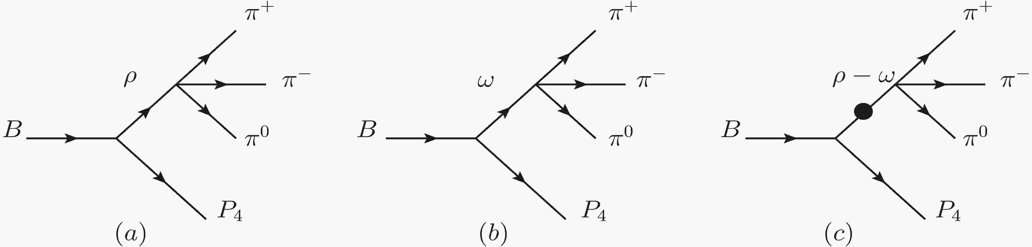
In order to explain the resonance effect, we use the $ B\rightarrow \omega(\rho)P_{4}\rightarrow \pi^{+}\pi^{-}\pi^{0}P_{4} $ decay channel as an example to study CP asymmetry, where $ P_{4} $ refers to the fourth final particle. The decay of B meson into $ \pi^{+}\pi^{-}\pi^{0}P_{4} $ is depicted in diagram (a) of Fig. 1, where the intermediate state ρ meson directly produces the final state $ \pi^{+}\pi^{-}\pi^{0} $. Meanwhile, the middle diagram (b) of Fig. 1 illustrates the decay of B meson into $ \pi^{+}\pi^{-}\pi^{0}P_{4} $, where the production of $ \pi^{+}\pi^{-}\pi^{0} $ is directly mediated by the ω meson. The existence of the $ \pi^{+}\pi^{-}\pi^{0} $ pair can also be attributed to the resonance effect originating from intermediate states involving ρ and ω mesons. However, due to G-parity violation in the decay process of $ \rho \rightarrow \pi^{+}\pi^{-}\pi^{0} $, the contribution of $ \omega \rightarrow \rho \rightarrow \pi^{+}\pi^{-}\pi^{0} $ is suppressed. Therefore, the decay process of $ \rho \rightarrow \omega \rightarrow \pi^{+}\pi^{-}\pi^{0} $ plays a crucial role in the mixing mechanism. Consequently, we investigate the processes involving the mixing of ρ and ω decays into $ \pi^{+}\pi^{-}\pi^{0} $, as depicted in diagram (c) of Fig. 1.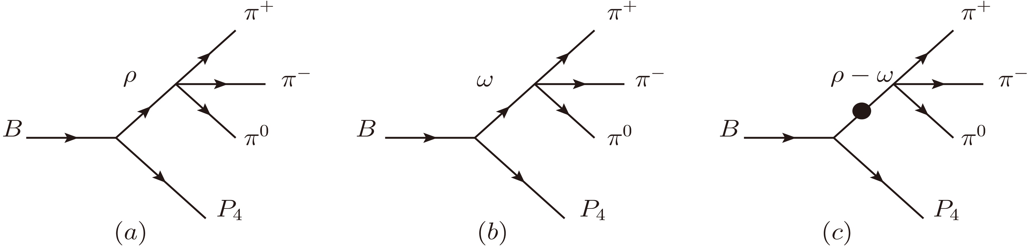

Figure 1.  The decay diagrams for the channel of $ B\rightarrow \omega(\rho)\pi^{0} \rightarrow \pi^{+}\pi^{-}\pi^{0}P_{4} $.

In QCDF approach, the non-perturbative contribution can be characterized by the universal distribution amplitude and form factor of mesons. The value of the form factor can be determined through semi-leptonic decay experiments of B mesons or by employing the QCDF method. Moreover, information regarding the light cone distribution amplitude of mesons can also be extracted from other hard scattering partial decay processes. While naive factorization yields leading-order decay amplitudes, radiation corrections to all orders, including chiral enhancement factors, can be calculated in the heavy quark limit by neglecting power corrections of 1/$ m_b $. We employ a quasi-two-body decay process to calculate the CP asymmetry. In the two-body decay of the B-meson, the form factor governing the transition from the initial hadron to the final hadron is dominated by non-perturbative effects [22]. We can calculate the perturbative contribution associated with the hard gluon from the QCD correction.

In the four-body decay process, we apply the narrow width approximation (NWA) to calculate the decay amplitude [23]. Hence, the relationship can be written as:

where V refers to the intermediate resonant vector meson. Γ and B are the decay width and branching fraction of the decay process, respectively. The decay amplitude of $ B\rightarrow VP_4 \rightarrow \pi^{+}\pi^{-}\pi^{0} P_{4} $ can be expressed as:

where $R_{\rm BW}$ is the Breit-Wigner propagator. M represents the the decay amplitudes, C refer to the $ \omega (\rho)\rightarrow \pi^+ \pi^- \pi^0 $ decay amplitudes associated with matrix elements. The four-body decay process can be described as a quasi-two-body decay, which can be evaluated using QCDF approach. In the following analysis, we will focus on the $ \omega (\rho)\rightarrow \pi^+ \pi^- \pi^0 $ decay process. For simplicity, we replace $ \omega (\rho)\rightarrow \pi^+ \pi^- \pi^0 $ with $ V\rightarrow 1,2,3 $. The double-differential decay rate are expressed as [24, 25]:

where $ C_{V\rightarrow123} $ is the decay amplitude associated with the matrix elements. P is the phase space factor $P= -\dfrac{1}{3}\epsilon_{\mu v \alpha \beta }p^{\mu}p^{v}_{1}p^{\alpha}_{2}\epsilon_{\overline{\mu} \overline{v} \overline{\alpha} \beta }p^{\overline{\mu}}p^{\overline{v}}_{1}p^{\overline{\alpha}}_{2}$. The relation between mass (m) and momentum (p) is is given by: $m^{2}_{ij}=(p_i+p_j)^2, M^2=p^2$, where $ p $ denotes the momentum of the vector meson and M represents the mass of the vector meson. We make an equivalent substitution for momentum and mass: $ q_1^2=m_{23}^2 $, $ q_3^2=m_{12}^2 $, $q_2^2=m_{13}^2=p^2-m^2_{12} - m^2_{23}+ p^2_1+ $ $p^2_2+p^2_3$, $ p=p_1+p_2+p_3 $. Additionally, $ m_{12} $ refer to the invariant mass of $ \pi^+ \pi^- $, $ m_{13} $ pertains to the invariant mass of $ \pi^+ \pi^0 $ and $ m_{23} $ signifies the invariant mass of $ \pi^- \pi^0 $. The amplitudes of the process $ \omega(\rho) \rightarrow \pi^+ \pi^- \pi^0 $ are determined by the matrix element:

The value of $ h_P $ is determined precisely through fitting the electromagnetic pion form factor, while the parameter f represents the pion-decay constant in the chiral limit which is on the order of GeV. The parameters $ h_A $ and $ b_A $ are determined by the radiation decay of vector mesons. By applying the Lagrangian equation, we constrain the combination of $ m_{V}h_{P}h_{A}/f^3 $ for vector meson decay into two pseudoscalar states. The values of the $ h_P $ parameters, fitted from experimental decay widths, are consistent within a range of ±10%. Furthermore, considering radiation decay in vector mesons, we determine the specific values of the following parameters [17]: $ h_{p}=0.304 $, $ h_{A}=2.1 $, $ f=0.09 $ and $ b_{A}=0.27 $.

Additionally, before performing integral operations, we provide a first-order calculation for hadronic three-body decay of vector mesons and estimate uncertainties based on $ \omega \rightarrow \pi^+ \pi^- \pi^0 $ decay analysis. In our two-body decay analysis, we determine the specific values of the above parameters of decay processes that have been proven to be associated with SU(3) flavor symmetry. The measurements of particle combinations are present in hadron two-body decay. To obtain a conservative error estimate, we use the largest error ±10% and assign it to the matrix element from the corresponding process to reduce the effect introduced by the error. Therefore, we use the energy-dependent meson width combined with the meson mass and momentum to define the propagators $ S_{\rho}(q^2) $ and $ S_{\omega}(q^2) $ in Eq. (16). The expressions of momenta dependent propagators $ S_{\rho}(q^2) $ and $ S_{\omega}(q^2) $ are obtained:

where the energy-dependent width of mesons is denoted by $ \Gamma_\rho(q^2) $ or $ \Gamma_\omega(q^2) $. $ \Gamma_{\rho}^{0} $ and $ \Gamma_{\omega}^{0} $ represent the on-shell width of ρ and ω mesons, respectively. Therefore, the decay amplitude of $ B\rightarrow VP_4 \rightarrow \pi^{+}\pi^{-}\pi^{0} P_{4} $ due to the quasi-two-body decays and QCDF can be expressed as

where $ V_{ub}V^{*}_{ud(s)} $ and $ V_{tb}V^{*}_{td(s)} $ are CKM matrix elements. The decay constants $ f^{q(s)}_{\eta^{(')}} $, $ f_{K(\pi)} $, $ f_{B} $ and $ f_{\omega(\rho)} $ correspond to the non-perturbative contributions, while the coefficients $a_{1,2,\cdots,n}$ are associated with the Wilson coefficients $ C_i $ [26]. The form factors for processes such as $ B\rightarrow \rho $ and $ B\rightarrow \omega $, denoted by $ A_0^{B\rightarrow \rho} $ and $ A_0^{B\rightarrow \omega} $, as well as those for processes like $ B\rightarrow \pi $ represented by $ F_1^{B\rightarrow \pi} $, arise from non-perturbative effects. Additionally, annihilation contributions given by $ b_3 $, $ b_3^{e\omega} $ and $ b_4^{e\omega} $ have been considered [27].Here $ \epsilon $ denotes the polarization vector of the meson and $ {p_\pi } $ represents momentum of the π. Furthermore, we define a mass parameter (m) which characterizes the quark mass related to the meson component in $ O_i $ [28, 29]:

We employ phenomenological parameters to express the endpoint integrals of these logarithmic divergences arising from the hard scattering process involving the spectator quark. Additionally, we incorporate the twist-3 distribution amplitude of the final pseudo-scalar meson in order to investigate the annihilation amplitude [29]. In the annihilation decay process, b is the annihilation coefficient where $ b_{1,2} $, $ b_{3,4} $ and $ b_{3,4}^{e\omega} $ correspond to the effective weak operators, $ Q_{1,2} $, QCD penguin operators $ Q_{3-6} $ and the weak electric penguin operator $ Q_{7-10} $, respectively [4]. We introduce the parameters $ X_H $ and $ X_A $, where $ X_{H} $ is defined as $\int_{0}^{1} {(1-y)^{-1}}{{\rm d}{y}}$ and $ X_{A} $ is defined as $\int_{0}^{1} {x}^{-1}{{\rm d}{x}}$, to account for the annihilation contribution. Subsequently, we incorporate the asymptotic form of the meson distribution amplitude into our solution, which cannot be disregarded [30]. The values of some parameters in the amplitude are provided as follow in Table 1.

$ f_{\omega}=0.195\pm0.005 $	$ f_{\rho}=0.216\pm0.003 $	$ f_{\pi}=0.131\pm0.009 $	$ f_{K}=0.155\pm0.002 $
$ f_{B}=0.18\pm0.04 $	$ f^q_{\eta^{(')}}=(1.07\pm0.02)f_\pi $	$ f^s_{\eta^{(')}}=(1.34\pm0.06)f_\pi $	$ F_{1}^{B\rightarrow \pi}=0.28\pm0.05 $
$ F_{1}^{B\rightarrow K}=0.31\pm0.02 $	$ F_{1}^{B\rightarrow \eta^{(')}}=0.132\pm0.003 $	$ A_{0}^{B\rightarrow \rho}=0.37\pm0.06 $	$ A_{0}^{B\rightarrow \omega}=0.281\pm0.04 $

Table 1.  Input parameter value.

The total amplitude used in the calculation is denoted by M, where M represents the sum of the tree-level contribution ($\big < \pi^{+}\pi^{-}\pi^{0}P_{4}|H^{\rm{T}}|B\big >$) and the penguin-level contribution ($ \big<\pi^{+}\pi^{-}\pi^{0}P_{4}|H^P|B\big> $). The phase angle, which affects the CP asymmetry in the decay process, is determined by the ratio of the penguin diagram contribution to that of the tree diagram. The expression can be written as follows [5]:

where the parameter r represents the ratio between the amplitude contributions of the penguin diagram and the tree diagram. The strong phase δ is generated through resonance effects and hadron matrix elements in this four-body decay process, while the weak phase ϕ is associated with the CKM matrix. These phases can significantly impact the CP asymmetry.

Furthermore, considering the interference between ρ and ω, we can present the detailed formalisms of the tree and penguin amplitude by combining the decay diagrams shown in Fig. 1.

where $ t_{\rho}(p_{\rho}) $ and $ t_{\omega}(p_{\omega}) $ are the ratios of the contributions from $ B\rightarrow \rho^{0}P_{4} $ and $ B \rightarrow \omega P_{4} $ decay processes, respectively. $ s $ is the invariant mass squared of mesons $ \pi^+\pi^-\pi^0 $ [25]. Besides, $ C_{\omega \rightarrow \pi^+ \pi^- \pi^0} $ and $ C_{\rho \rightarrow \pi^+ \pi^- \pi^0} $ are calculated in Eq. (14) and Eq. (15), respectively. We can now proceed to obtain the following relations:

where $ \delta_\lambda $, $ \delta_\alpha $ and $ \delta_\beta $ are strong phases. Substituting these into Eq. (29) and Eq. (30), and simplifying, we obtain:

The phase ϕ is determined by the ratio of $ V_{ub}V^{*}_{ud} $($ V_{ub}V_{us}^{*} $) to $ V_{tb}V^{*}_{td} $($ V_{tb}V_{ts}^{*} $) in the CKM matrix. Hence, we can derive $ {\rm{sin}}\phi = \frac{\eta}{\sqrt{(\rho-\rho^2-\eta^2)^2+\eta^2}} $($ {\rm{sin}}\phi = -\frac{\eta}{\sqrt{\rho^2+\eta^2}} $) and ${\rm{cos}}\phi = \frac{\rho-\rho^2-\eta^2}{\sqrt{(\rho-\rho^2-\eta^2)^2+\eta^2}}$($ {\rm{cos}}\phi = -\frac{\rho}{\sqrt{\rho^2+\eta^2}} $) using Wolfenstein parameters [19]. Subsequently, we define the CP asymmetry as follows: $ A_{cp} = \frac{\left| M \right|^2 - \left| \overline{M} \right|^2}{\left| M \right|^2 + \left| \overline{M} \right|^ 2} $.

We consider the resonance effect that generates a new strong phase and influences the CP asymmetry. However, to obtain a more accurate result, we need to integrate the $A_{\rm CP}$ over the phase space. Since ω meson is usually reconstructed through the decay channel $ \omega \rightarrow \pi^+ \pi^- \pi^0 $, the localised CP asymmetry $ A_{\rm CP}^{\Omega} $ of $ B \rightarrow \pi^+ \pi^- \pi^0 P_{4} $ with invariant mass near the ω resonance can be expressed as [11, 31]:

The equation involves the decay amplitude of $ B\rightarrow \pi^+\pi^-\pi^0 P_{4} $, where $ M^{\pm} $ represents it. The squared invariant masses of the systems $ m^2_{\pi^+\pi^-} $, $ m^2_{\pi^-\pi^0} $ and $ m^2_{\pi^+\pi^-\pi^0} $ are denoted by $ m^2_{12} $, $ m^2_{23} $ and $ m^2_{123} $, respectively. Besides, integral limit set in the $ (m_{\omega+\Delta\omega})^2 $ and $ (m_ {\omega-\Delta\omega})^2 $ in the vicinity of ω mass. Here the range of $ m_{\omega+\Delta\omega} $ and $ m_{\omega-\Delta\omega} $ values varies within a small range near ω mass. The mass of the ω meson is denoted as $ m_{\omega} $. The value of $ \Delta\omega $ is chosen such that the line shape of $ \omega $ is included in the integral interval. When reconstructing the ω meson experimentally, the cut $ \Delta\omega $ is selected to optimize the signal-to-background ratio by considering the convolution for the width of the ω meson and the momentum resolution of the detector. Typically, $ \Delta\omega $ is comparable to the decay width $ \Gamma_{\omega} $ of the ω meson, which has been confirmed in previous studies from the ALICE collaboration [23, 32] and we also selected a threshold interval similar to the test in the following calculation.

We thoroughly consider the previous experimental findings and perform calculations on the resonance effect of vector meson mixing. Consequently, the results are presented in Fig. 2−Fig. 10, which illustrate the interrelation between CP asymmetry (denoted by r and the strong phase δ) and the energy $ \sqrt{s} $. Based on the Particle Data Group (PDG) data, the masses of ρ and ω are approximately estimated to be 0.770 GeV and 0.782 GeV, respectively [17]. To visualize the resonance effect around mass ω, we choose the region 0.70−0.90 GeV under our theoretical framework. The plots in Figs. 2–10 correspond to this region, which is the main resonance region for the decay process $ \omega(\rho)\rightarrow \pi^{+}\pi^{-}\pi^{0} $. The invariant mass of $ \pi^{+}\pi^{-}\pi^{0} $ is displayed in the vicinity of the ω meson's mass. By selecting this range, we can effectively observe the overall CP asymmetry [33]. From the plots, we see that the CP asymmetry changes drastically for the $ \bar{B}^{0}\rightarrow \pi^{+}\pi^{-}\pi^{0}\pi^{0}(\bar K^{0}, \eta,\eta^{'}) $ and $ B^{-} \rightarrow \pi^{+}\pi^{-}\pi^{0}\pi^{-}( K^{-}) $ decay modes due to the $ \rho\rightarrow \pi^{+}\pi^{-}\pi^{0} $ and $ \omega\rightarrow \pi^{+}\pi^{-}\pi^{0} $ resonances in Fig. 2, Fig. 3 and Fig. 4 where ω dominates.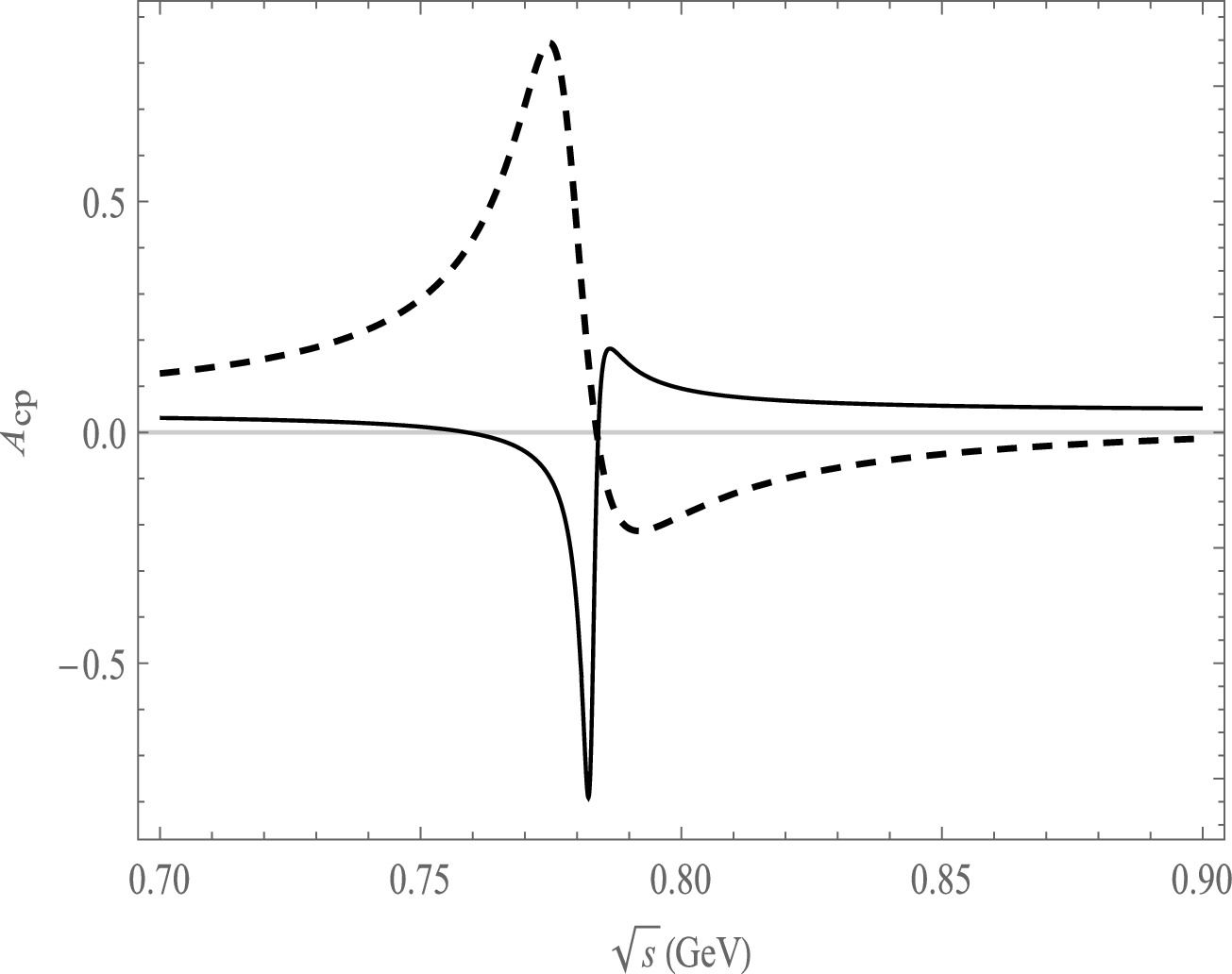

Figure 2.  Plot of $A_{\rm CP}$ as a function of $ \sqrt{s} $, the solid line is the decay channel of $ \bar B^{0}\rightarrow \pi^{+}\pi^{-}\pi^{0}\pi^{0} $, the dash line is the decay channel of $ \bar B^{0}\rightarrow \pi^{+}\pi^{-}\pi^{0}\bar K^{0} $.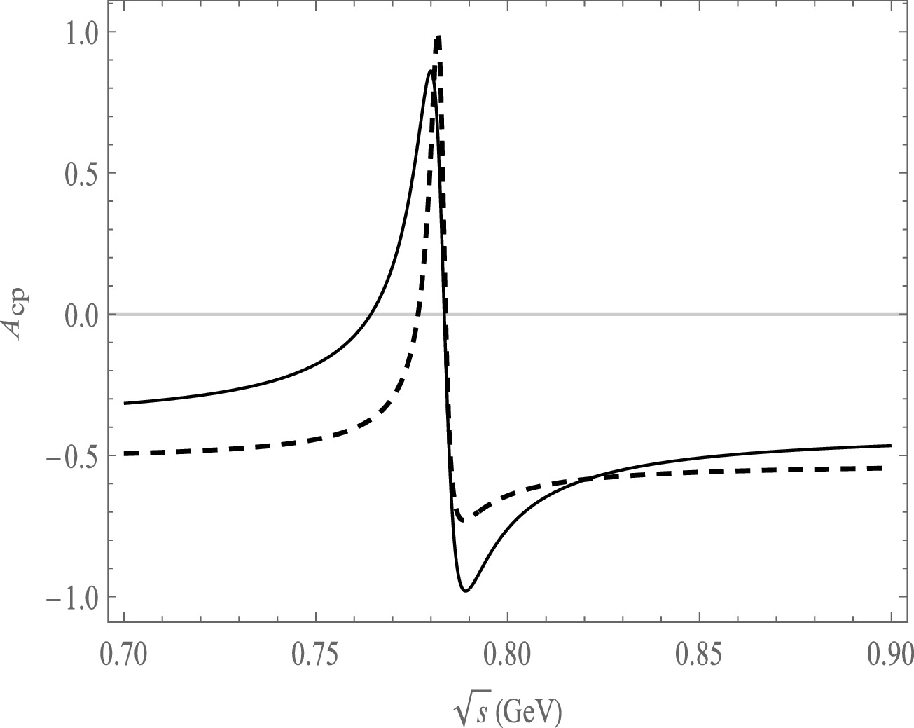

Figure 3.  Plot of $A_{\rm CP}$ as a function of $ \sqrt{s} $, the solid line is the decay channel of $ \bar B^{0}\rightarrow \pi^{+}\pi^{-}\pi^{0}\eta $, the dash line is the decay channel of $ \bar B^{0}\rightarrow \pi^{+}\pi^{-}\pi^{0}\eta^{'} $.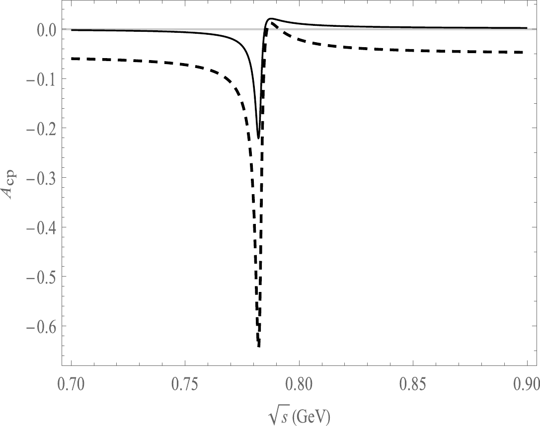

Figure 4.  Plot of $A_{\rm CP}$ as a function of $ \sqrt{s} $, the solid line is the decay channel of $ B^{-}\rightarrow \pi^{+}\pi^{-}\pi^{0}\pi^{-} $, the dash line is the decay channel of $ B^{-}\rightarrow \pi^{+}\pi^{-}\pi^{0}K^{-} $.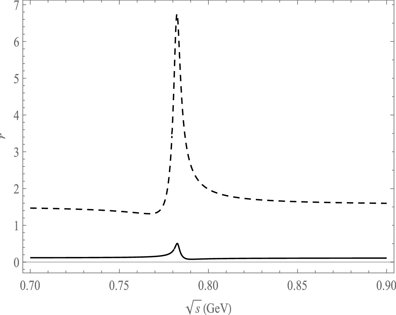

Figure 5.  Plot of $ r $ as a function of $ \sqrt{s} $, the solid line is the decay channel of $ \bar B^{0}\rightarrow \pi^{+}\pi^{-}\pi^{0}\pi^{0} $, the dash line is the decay channel of $ \bar B^{0}\rightarrow \pi^{+}\pi^{-}\pi^{0}\bar K^{0} $.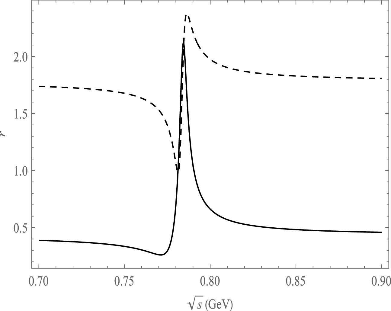

Figure 6.  Plot of $ r $ as a function of $ \sqrt{s} $, the solid line is the decay channel of $ \bar B^{0}\rightarrow \pi^{+}\pi^{-}\pi^{0}\eta $, the dash line is the decay channel of $ \bar B^{0}\rightarrow \pi^{+}\pi^{-}\pi^{0}\eta^{'} $.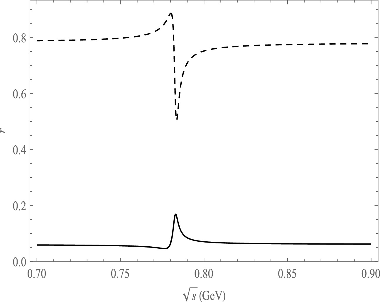

Figure 7.  Plot of $ r $ as a function of $ \sqrt{s} $, the solid line is the decay channel of $ B^{-}\rightarrow \pi^{+}\pi^{-}\pi^{0}\pi^{-} $, the dash line is the decay channel of $ B^{-}\rightarrow \pi^{+}\pi^{-}\pi^{0}K^{-} $.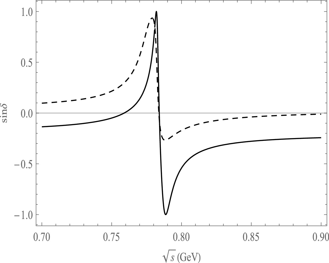

Figure 8.  Plot of $ {\rm{sin}}\delta $ as a function of $ \sqrt{s} $, the solid line is the decay channel of $ \bar B^{0}\rightarrow \pi^{+}\pi^{-}\pi^{0}\pi^{0} $, the dash line is the decay channel of $ \bar B^{0}\rightarrow \pi^{+}\pi^{-}\pi^{0}\bar K^{0} $.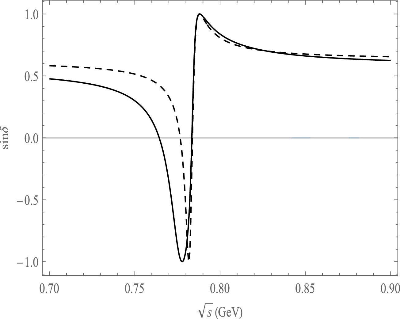

Figure 9.  Plot of $ {\rm{sin}}\delta $ as a function of $ \sqrt{s} $, the solid line is the decay channel of $ \bar B^{0}\rightarrow \pi^{+}\pi^{-}\pi^{0}\eta $, the dash line is the decay channel of $ \bar B^{0}\rightarrow \pi^{+}\pi^{-}\pi^{0}\eta^{'} $.

For the $ \bar{B}^{0}\rightarrow \pi^{+}\pi^{-}\pi^{0}\pi^{0} $ decay mode, significant CP asymmetries ranging from $ -78.5 $% to 18.2% are observed in the resonance regions of ρ and ω, as shown in Fig. 2. In the case of $ \bar{B}^{0}\rightarrow \pi^{+}\pi^{-}\pi^{0}\bar K^{0} $ decay, large CP asymmetries ranging from 84.2% to $-21.9$% are found in the same resonance regions of ρ and ω, as depicted in Fig. 2. So it is noteworthy that there is a large change in CP asymmetry between the two decay modes: $\bar{B}^{0}\rightarrow \pi^{+}\pi^{-}\pi^{0}\bar K^ {0}$ and $ \bar{B}^{0}\rightarrow \pi^{+}\pi^{-}\pi^{0}\pi^{0} $.

We also observe CP asymmetries in the decay channel $ \bar B^{0}\rightarrow \pi^{+}\pi^{-}\pi^{0}\eta $ ranging from $ -98.3 $% to 86.0% within the resonance range of ρ and ω, as shown in Fig. 3. In the case of $ \bar B^{0}\rightarrow \pi^{+}\pi^{-}\pi^{0}\eta' $, we find significant CP asymmetries ranging from $ -73.1 $% to 98.9% within the same resonance region depicted in Fig. 3. The CP asymmetries in the decay channel $\bar B^{0}\rightarrow \pi^{+}\pi^{-}\pi^{0}\eta{'}$ exhibit a pronounced variation similar to that observed in the decay process of $ \bar B^{0}\rightarrow \pi^{+}\pi^{-}\pi^{0}\eta $, specifically within the mass resonances of ω(ρ).

On the other hand, we obtain CP asymmetries ranging from $ -21.8 $% to 2.26% in the ρ and ω resonance range for the decay channel $ B^{-}\rightarrow \pi^{+}\pi^{-}\pi^{0}\pi^{-} $ as shown in Fig. 4. The CP asymmetries range from $ -64.5 $% to 1.30% in the decay channel of $ B^{-}\rightarrow \pi^{+}\pi^{-}\pi^{0}K^{-} $ which also has a large change in the CP asymmetry in the resonance of ρ and ω mass. We can see that the resonance effect is mainly around the ρ and ω mass range for all the decay channels.

The ratio r of the penguin-level contribution and tree-level contribution influences the CP asymmetry. The relationship between r and $ \sqrt{s} $ using the central parameter values of the CKM matrix elements in Fig. 5, Fig. 6 and Fig. 7. The variation range of r in the ω and ρ resonance ranges is not significant for the decay mode of $ B\rightarrow \pi^{+}\pi^{-}\pi^{0}\pi^{0}(\pi^-) $. We also notice that r varies significantly at the ω mass region from the decay modes of $ B\rightarrow \pi^{+}\pi^{-}\pi^{0}\bar K^{0}(\eta,\eta^{'},K^-) $.

In the calculation of CP asymmetry, the strong phase δ is taken into account, and its definition is given in Eq. (32). The variation of the strong phase also affects CP asymmetry. We present the plots of $ {\rm{sin}}\delta $ versus $ \sqrt{s} $ based on the central values of the CKM matrix elements, as depicted in Figs. 8, 9, and 10. These figures illustrate the dependence of CP asymmetry on the strong phase. In Fig. 8, we can clearly observe the variation of $ {\rm{sin}}\delta $ in the ρ and ω resonance regions for the $\bar B^{0}\rightarrow \pi^{+}\pi^{-}\pi^{0}\pi^{0}(\bar K^0)$ decay mode. Similarly, in Fig. 9 and Fig. 10, we observe $ {\rm{sin}}\delta $ significant changes in the ρ and ω resonance regions for the decay modes of $\bar B^{0}\rightarrow \pi^{+}\pi^{-}\pi^{0}\eta(\eta^{'})$ and $B^{-}\rightarrow \pi^{+}\pi^{-}\pi^{0}\pi^{-}(K^{-})$.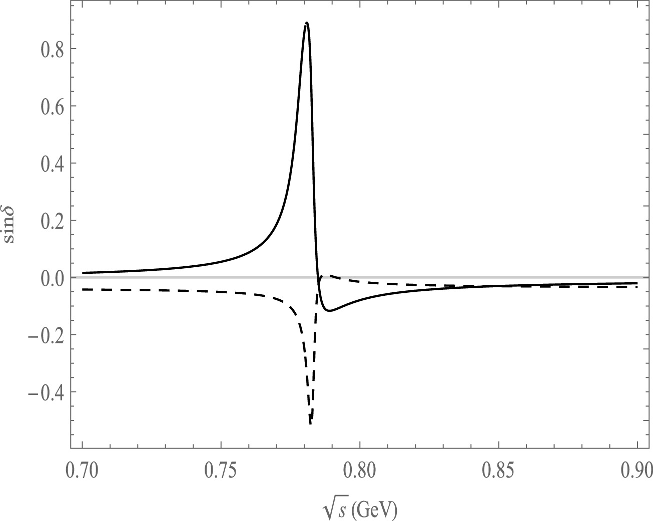

Figure 10.  Plot of $ {\rm{sin}}\delta $ as a function of $ \sqrt{s} $, the solid line is the decay channel of $ B^{-}\rightarrow \pi^{+}\pi^{-}\pi^{0}\pi^{-} $, the dash line is the decay channel of $ B^{-}\rightarrow \pi^{+}\pi^{-}\pi^{0}K^{-} $.

The CP asymmetries are influenced by the non-zero complex phase ϕ in the CKM matrix, strong phase δ and the absolute value r of the ratio of the penguin and tree amplitudes. In the framework of QCDF method, we calculate the decay amplitudes from Eq. (17) to Eq. (26) due to quasi-two-body decay process. It can be seen that the decay amplitudes depend on the CKM matrix elements, decay constants, form factors, and Wilson coefficients for different final state particles. The strong phase δ and the absolute value r of the ratio of the penguin and tree amplitudes can be calculated from the method of QCDF which is different for different final state particle. Hence, the CP asymmetries differ across various decay channels, as seen in Figs. 2, 3, and 4.

The measurement of CP asymmetry in B meson decays has significantly advanced in recent years due to the extensive accumulation of experimental data [34]. The invariant differential cross section of inclusive $ \omega(782) $ meson production at midrapidity ($ |y|<0.5 $) in pp collisions at $ \sqrt{s}=7 $ TeV was measured utilizing the ALICE detector at the Large Hadron Collider across a transverse momentum range of $ 2 < p_T < 17 $ GeV/c. The ω meson was reconstructed through its decay to $ \pi^{+}\pi^{-}\pi^{0} $, where the $ \pi^{0} $ subsequently decays into two photons. This approach required the reconstruction of charged tracks within the ALICE central tracking system, which consists of the inner tracking system (ITS) and the time projection chamber (TPC). Additionally, photons were reconstructed using the electromagnetic calorimeter (EMCal) and the photon spectrometer (PHOS), with the photon conversion method (PCM) used to reconstruct photons from electron–positron track pairs. For further details on the ALICE detector system and its performance, the reader is referred to Refs.[35−38].

Combined with the experimental observation interval, we select the energy range of CP asymmetry producing peak value in the plot, and integrate the CP asymmetry results in this region. In our work, we are the first to calculate the CP asymmetry for the $ \bar B^{0}\rightarrow \omega \bar K^{0}(\pi^{0}) \rightarrow \pi^{+}\pi^{-}\pi^{0}\bar K^{0}(\pi^{0}) $, $ \bar B^{0}\rightarrow \omega \eta(\eta^{'}) \rightarrow \pi^{+}\pi^{-}\pi^{0}\eta(\eta^{'}) $ and $B^{-}\rightarrow \omega K^{-}(\pi^-)\rightarrow \pi^{+}\pi^{-}\pi^{0}K^{-}(\pi^-)$ decay modes by integrating over the invariant masses of $ m_{\pi^{+}\pi^{-}\pi^{0}} $ in the range of 0.75−0.82 GeV from the ρ and ω resonance regions since the mass of ρ is 0.770 GeV and the mass of ω is 0.782 GeV [23].

The formula for the rate of change of the local integral is defined as $({A^\Omega _{cp1}-A^\Omega _{cp2}})/{A^\Omega _{cp1}}$, where $A^\Omega _{cp1}$ is the CP asymmetry result without mixing and $ A^\Omega _{cp2} $ is the CP asymmetry result with mixing. The results and rate of change are summarized in Table 2. We observe that the resonance effect significantly affects the CP asymmetry results for the decay processes $ B\rightarrow \pi^{+}\pi^{-}\pi^{0}P_4 $. Additionally, the rate of change for the local integral in the range 0.75−0.82 GeV provides a clear view of the influence of the resonance effect on CP asymmetry [39]. In Table 2, one can see that the rates of change are large for the processes $ \bar B^{0}\rightarrow \omega(\rho) \pi^{0} \rightarrow \pi^{+}\pi^{-}\pi^{0}\pi^{0} $ and $B^{-}\rightarrow \omega(\rho)K^{-} \rightarrow \pi^{+}\pi^{-}\pi^{0}K^{-}$ comparing with direct decay through ω meson. The mixing results exhibit two sources of uncertainty within the resonance mechanism in our work. The first uncertainty arises from the decay width and the Wolfenstein parameters, while the second is due to the QCDF method, which introduces some error in the parameters themselves.

Decay channel	Without $\omega-\rho$ mixing (0.75−0.82 GeV)	$\omega-\rho$ mixing (0.75−0.82 GeV)	Rate of change
$ \bar B^{0}\rightarrow \omega(\rho) \pi^{0} \rightarrow \pi^{+}\pi^{-}\pi^{0}\pi^{0} $	0.095$ \pm $0.005$ \pm $0.007	–0.004$ \pm $0.007$ \pm $0.011	95.78%
$ \bar B^{0}\rightarrow \omega(\rho) \bar K^{0} \rightarrow \pi^{+}\pi^{-}\pi^{0}\bar K^{0} $	–0.140$ \pm $0.012$ \pm $0.011	0.107$ \pm $0.032$ \pm $0.041	23.57%
$ \bar B^{0}\rightarrow \omega(\rho) \eta \rightarrow \pi^{+}\pi^{-}\pi^{0}\eta $	–0.469$ \pm $0.007$ \pm $0.014	–0.358$ \pm $0.009$ \pm $0.001	23.66%
$ \bar B^{0}\rightarrow \omega(\rho) \eta^{'} \rightarrow \pi^{+}\pi^{-}\pi^{0}\eta^{'} $	–0.582$ \pm $0.006$ \pm $0.007	–0.477$ \pm $0.005$ \pm $0.016	18.04%
$ B^{-}\rightarrow \omega(\rho) \pi^{-} \rightarrow \pi^{+}\pi^{-}\pi^{0}\pi^{-} $	0.015$ \pm $0.003$ \pm $0.004	–0.012$ \pm $0.003$ \pm $0.009	20.01%
$ B^{-}\rightarrow \omega(\rho)K^{-} \rightarrow \pi^{+}\pi^{-}\pi^{0}K^{-} $	–0.089$ \pm $0.008$ \pm $0.012	–0.010$ \pm $0.009$ \pm $0.011	88.76%

Table 2.  The comparison of $ A^\Omega _{cp} $ from $ \omega-\rho $ mixing with $ \omega \rightarrow \pi^{+}\pi^{-}\pi^{0} $.

In this work, we have demonstrated that CP asymmetries exhibit significant variation due to the resonance effect of $ V\rightarrow \pi^{+}\pi^{-}\pi^{0} $ $ (V=\rho, \omega) $ in the $ B \rightarrow \pi^{+}\pi^{-}\pi^{0}\pi (K,\eta^{(')}) $ decay modes when the invariant mass of $ \pi^{+}\pi^{-}\pi^{0} $ is close to the ρ and ω resonance regions within the framework of QCD factorization. The interference of $ \rho-\omega $ generates new strong phases that influence the CP asymmetry from the $ B \rightarrow \pi^{+}\pi^{-}\pi^{0}\pi(K,\eta^{(')}) $ decay rates. The resonance effect plays a critical role on the CP asymmetry under the mixing of the ρ and ω. We also calculated the localized CP asymmetry by integrating $ B \rightarrow \omega(\rho)P_{4} \rightarrow \pi^{+}\pi^{-}\pi^{0}P_{4} $, over specific phase space regions corresponding to these resonance effects. This localized CP asymmetry undergoes a significant change due to the resonances of ρ and ω, which arise from the G-parity suppressed decay process of $ \rho^{0} \rightarrow \pi^{+}\pi^{-}\pi^{0} $.

We calculate the CP asymmetry in the decay process by employing an energy variation interval for ω that closely aligns with experimental observations. Subsequently, we conducted a comparative analysis of our mixed and non-mixed results to identify any disparities between the decay processes. Notably, the resonance effect exerts a significant influence on the CP asymmetry within the same energy range. In particular, the rates of change for the CP asymmetry resulting from the mixing mechanism in these two decay processes, $ \bar{B}^{0}\rightarrow \omega(\rho)\pi^{0} \rightarrow \pi^{+}\pi^{-}\pi^{0}\pi^{0} $ and $ B^{-}\rightarrow \omega(\rho) K^{-} \rightarrow \pi^{+}\pi^{-}\pi^{0}K^{-} $, can attain values of 95.78% and 88.76%, respectively, which are larger than that produced by the others decay processes. We can reconstruct the ρ and ω mesons from the final state mesons of $ \pi^{+}\pi^{-}\pi^{0} $ to validate the predicted CP asymmetries. We anticipate that these results will contribute to the ongoing experimental efforts to explore CP violation in B meson decays, offering insights into the dynamics of weak decays and resonance phenomena.