


 Abstract
 HTML
HTML Reference
 Related
 PDF
PDF


-
In 2003, a milestone in the exploration of the mico-world was reached by the observation of X(3872) [1]. Since then, numerous new hadronic states or candidates, denoted as
$ XYZ $ , have been observed in experiments, but these novel hadronic states cannot be well understood by the conventional quark model [2, 3]. Investigation of these new hadronic states can not only deepen our understanding of strong interaction but also enrich our knowledge of hadron spectroscopy, which is attracting increasing interest from theorists and experimentalists.To date, most new hadronic states observed by experiments possess the regular quantum number, while only a few of them have exotic
$ J^{PC} $ , although many theoretical investigations on exotic hadronic states have been made, including tetraquarks [4–12], hybrid tates [13–17], and glueballs [18–23]. With the development of technology, exotic hadronic states have gradually been observed in experiments, such as the most recently observed$ \eta_1(1855) $ [24, 25]. It is highly expected that more exotic new hadronic structures will emerge soon.As the
$ 0^{--} $ novel hadronic states are relatively light and their quantum number enables their production in the decays of vector quarkonium or quarkoniumlike states easier, special attention should be paid to these. However, no signal of$ 0^{--} $ states has been observed in experiments so far [26]. In Ref. [10],$ 0^{--} $ tetraquarks in diquark-antidiquark configuration were studied in the framework of QCD sum rules (QCDSR). In practice, there may exist another type of tetraquark in molecular configuration. In this paper, the$ 0^{--} $ molecular hidden-heavy tetraquark states are investigated via QCDSR.The QCD sum rule technique [27], as a model-independent approach in the study of hadron physics, has some peculiar advantages in exploring hadron properties involving nonperturbative QCD. The first step to establish the QCD sum rules is to construct the proper interpolating currents corresponding to the hadrons of interest. The interpolating currents should possess information about the quantum numbers and structural components of the concerned hadrons. By interpolating currents, we can construct the two-point correlation function with two representations, i.e., the operator product expansion (OPE) representation and phenomenological representation. Matching two sides of the two-point correlation, the hadron mass may be calculated by establishing the QCD sum rules.
The remainder of this paper is organized as follows. In Sec. II, a brief interpretation of QCD sum rules and some primary formulas in our calculation are presented. The numerical analysis and numerical results are given in Sec. III. Finally, Sec. IV presents a brief summary and discusses the possible decay modes of the
$ 0^{--} $ tetraquark states. -
The interpolating currents of the lowest order ones for
$ 0^{--} $ tetraquark state in molecular configuration can be constructed as follows:$ j_A(x)= {\rm i} [\bar{Q}_a(x) \gamma_\mu Q_a(x)][\bar{q}_b (x) \gamma^\mu\gamma_5 q_b(x)] \;, $

(1) $ j_B(x)= {\rm i}[\bar{Q}_a(x) \gamma_\mu\gamma_5 Q_a(x)][\bar{q}_b (x) \gamma^\mu q_b(x)] \;, $

(2) $ \begin{aligned}[b] j_C(x) =\;& \frac{\rm i}{\sqrt{2}}\big{\{}[\bar{Q}_a(x) \gamma_\mu q_a(x)][\bar{q}_b (x) \gamma^\mu\gamma_5 Q_b(x)]\\ &+[\bar{Q}_a(x) \gamma_\mu\gamma_5 q_a(x)][\bar{q}_b (x) \gamma^\mu Q_b(x)]\big{\}} \;, \end{aligned} $

(3) $ \begin{aligned}[b] j_D(x) =\;& \frac{\rm i}{\sqrt{2}}\big{\{}[\bar{Q}_a(x) \gamma_5 q_a(x)][\bar{q}_b (x) Q_b(x)]\\ &-[\bar{Q}_a(x) q_a(x)][\bar{q}_b (x) \gamma_5 Q_b(x)]\big{\}} \;. \end{aligned} $

(4) Here, the subscripts a and b are color indices, q represents light quark u or d, and Q represents the heavy quarks. Hereafter, for simplicity, the currents in Eqs. (1)–(4) will be referred as cases A to D, respectively.
Inputing currents (1)–(4) into the two-point correlation function, we get
$ \Pi_k(q^2) = {\rm i} \int {\rm d}^4 x\; {\rm e}^{{\rm i} q \cdot x} \langle 0 | T \{ j_k(x),\; j_k (0)^\dagger \} |0 \rangle \;, $

(5) where
$ |0 \rangle $ denotes the physical vacuum, and k runs from A to D. The OPE side of the correlation function$ \Pi(q^2) $ can be expressed as a dispersion relation:$ \Pi^{\rm OPE}_k (q^2) = \int_{s_{\min}}^{\infty} {\rm d} s\frac{\rho^{\rm OPE}_k(s)}{s - q^2}+\Pi^{\rm sum}_k(q^2)\, . $

(6) Here,
$s_{\min}$ is the kinematic limit, which usually corresponds to the square of the sum of current-quark masses of the hadron [28],$\rho^{\rm OPE}(s) = {\rm{Im}} [\Pi^{\rm OPE}(s)] / \pi$ , and can be expressed as$ \begin{aligned}[b] \rho^{\rm OPE}(s) =\;& \rho^{\rm pert}(s) + \rho^{\langle \bar{q} q \rangle}(s) +\rho^{\langle G^2 \rangle}(s) + \rho^{\langle \bar{q} G q \rangle}(s) \\&+ \rho^{\langle \bar{q} q \rangle^2}(s) +\rho^{\langle G^3 \rangle}(s) + \rho^{\langle \bar{q} q \rangle\langle \bar{q} G q \rangle}(s) \;. \end{aligned} $

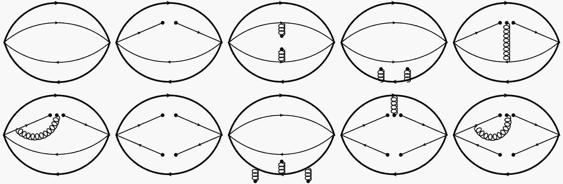
(7) $\Pi^{\rm sum}(q^2)$ is the sum of the contributions in the correlation function that have no imaginary part but are nontrivial after the Borel transformation.The Feynman diagrams corresponding to each term of Eq. (7) are schematically shown in Fig. 1. The analytical expressions of
$\rho^{\rm OPE}(s)$ can be found in Appendix A.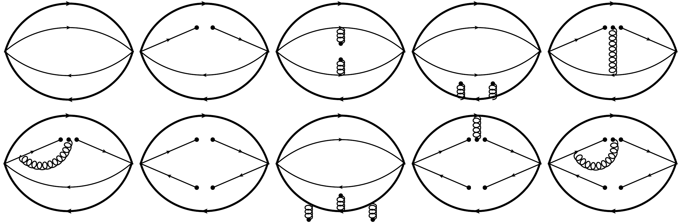
Figure 1. Typical Feynman diagrams related to the correlation function, where the thick solid line represents the heavy quark, the thin solid line represents the light quark, and the spiral line denotes the gluon. There is no heavy quark consendsate due to the large heavy quark mass.
On the phenomenological side, we can separate out the ground state contribution from the pole contribution of the correction function and express
$ \Pi(q^2) $ as a dispersion integral over the physical regime, i.e.,$ \Pi^{\rm phen}_k(q^2) = \frac{{\lambda_k}^2}{{M_k}^2 - q^2} + \int_{s_0}^\infty {\rm d} s \frac{\rho_k(s)}{s - q^2} \, , $

(8) where M, λ, and
$ \rho(s) $ represent the tetraquark mass, coupling constant of current to hadron, and spectral density that contains the contributions from higher excited states and continuum states above the threshold$ s_0 $ , respectively; the subscript i runs from A to D.Using quark–hadron duality, i.e., equating the OPE side and phenomenological side of the correlation function
$ \Pi(q^2) $ , i.e., Eqs. (6) and (8), and then performing the Borel transform, the QCD sum rule for the mass of$ 0^{--} $ tetraquark states is determined to be$ M(s_0, M_B^2) = \sqrt{- \frac{L_{1}(s_0, M_B^2)}{L_{0}(s_0, M_B^2)}} \; . $

(9) Here,
$ L_0 $ and$ L_1 $ are respectively defined as$ L_{0}(s_0, M_B^2) = \int_{s_{\min}}^{s_0} {\rm d} s \; \rho^{\rm OPE}(s) {\rm e}^{- s / M_B^2} +\Pi^{\rm sum}(M_B^2) \;$

(10) and
$ L_{1}(s_0, M_B^2) = \frac{\partial}{\partial{({1}/{M_B^2})}}{L_{0}(s_0, M_B^2)} \; . $

(11) -
In performing the numerical calculation, we use the values of the quark masses and condensates from [28–36], i.e.,
$ m_s=(95\pm5)\; {\rm{MeV}} $ ,$m_c (m_c) = \overline{m}_c= (1.275 \pm 0.025) \;\; {\rm{GeV}}$ ,$ m_b (m_b) = \overline{m}_b= (4.18 \pm 0.03) \; {\rm{GeV}} $ ,$ \langle \bar{q} q \rangle = - (0.23 \pm 0.03)^3 \; {\rm{GeV}}^3 $ ,$ \langle \bar{q} g_s \sigma \cdot G q \rangle = m_0^2 \langle\bar{q} q \rangle $ ,$ \langle g_s^2 G^2 \rangle = (0.88\pm0.25) \; {\rm{GeV}}^4 $ ,$ \langle g_s^3 G^3 \rangle = (0.045\pm0.013) \; {\rm{GeV}}^6 $ , and$ m_0^2 = (0.8 \pm 0.2) \; {\rm{GeV}}^2 $ . For light quarks u and d, the chiral limit masses$ m_u=m_d=0 $ were adopted.In establishing the QCD sum rules, two additional parameters, appropriate threshold
$ s_0 $ and Borel parameter$ M_B^2 $ , need to be introduced. We can select them by the so-called standard procedures by fulfilling the following two criteria in Refs. [27, 28, 36, 37]. The first is the convergence of the OPE, which is essential to compare the relative contribution of the higher dimension condensate to the total contribution on the OPE side; this can be formulated as$ R^{\rm OPE}= \left| \frac{L_{0}^{dim=8}(s_0, M_B^2)}{L_{0}(s_0, M_B^2)}\right|\, . $

(12) In practice, the criterion of the OPE convergence requires that the relative contribution of the highest dimension should be less than
$ 0.2 $ [36]. The second criterion of QCD sum rules requires that the pole contribution (PC) is more than 50% of the total [28, 32], which can be formulated as$ R^{PC} = \frac{L_{0}(s_0, M_B^2)}{L_{0}(\infty, M_B^2)} \; . $

(13) To find a proper value for continuum threshold
$ s_0 $ , a similar analysis as in Refs. [38–40] is performed. Therein, we need to pick up the$ \sqrt{s_0} $ , which yields an optimal window for Borel parameter$ M_B^2 $ . That is, the tetraquark mass M is approximately independent of the$ M_B^2 $ in this window. In practice, the lower and upper bounds of$ \sqrt{s_0} $ can be obtained by varying$ \sqrt{s_0} $ by$ 0.1 $ GeV and hence the uncertainties of$ \sqrt{s_0} $ [41, 42].With the above preparation, we can numerically calculate the mass spectrum of tetraquaek states. As an example, the OPE convergence and the PC for the tetraquark A are drawn in Fig. 2(a). According to the first criterion, it is found the lower limit of
$ M_B^2 $ is$ M_B^2 \ge 2.8\; {\rm{GeV}}^2 $ with an$ \sqrt{s_0} $ value of$ 5.1 $ GeV. The PC gives the upper bound for$ M_B^2 $ , i.e.,$ M_B^2 \le 3.4\; {\rm{GeV}}^2 $ with$ \sqrt{s_0}=5.1 $ GeV. Thus, the optimal Borel window is in the range$ 2.8 \le M_B^2 \le 3.4\; {\rm{GeV}}^2 $ , and the mass$ M^{A} $ can then be obtained as follows: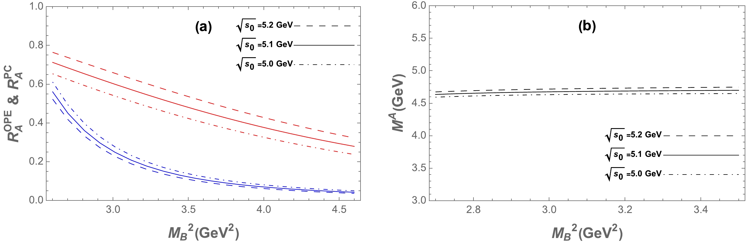
Figure 2. (color online) (a) Ratios of
${R_{A}^{\rm OPE}}$ and${R_{A}^{\rm PC}}$ as functions of the Borel parameter$ M_B^2 $ for different values of$ \sqrt{s_0} $ , where blue lines represent${R_{A}^{\rm OPE}}$ , and red lines denote${R_{A}^{\rm PC}}$ . (b) Mass$ M^{A} $ as a function of the Borel parameter$ M_B^2 $ for different values of$ \sqrt{s_0} $ .$ M^{A} = (4.68\pm 0.07)\; {\rm{GeV}}. $

(14) Similarly, we can evaluate the masses of the
$ 0^{--} $ tetraquarks B-D as$ M^{B} = (4.22\pm 0.09)\; {\rm{GeV}}. $

(15) $ M^{C} = (4.53\pm 0.09)\; {\rm{GeV}}. $

(16) $ M^{D} = (4.26\pm 0.13)\; {\rm{GeV}}, $

(17) with the OPE, pole contribution, and masses as functions of Borel parameter
$ M_B^2 $ given in Appendix B. The errors in results (14)−(17) mainly stem from the uncertainties in quark masses, condensates, and threshold parameter$ \sqrt{s_0} $ . For convenience of reference, a collection of continuum thresholds, Borel parameters, and predicted masses of$ 0^{--} $ tetraquark states are listed in Table 1.Current $\sqrt{s_0}/{\rm{GeV} }$ 

$M_B^2 /{\rm{GeV} }^2$ 

$M^X /{\rm{GeV} }$ 

c-sector A $ 5.1\pm0.1 $ 

$ 2.8-3.4 $ 

$ 4.68\pm0.07 $ 

B $ 4.7\pm0.1 $ 

$ 2.2-2.8 $ 

$ 4.22\pm0.09 $ 

C $ 5.0\pm0.1 $ 

$ 2.6-3.2 $ 

$ 4.53\pm0.09 $ 

D $ 4.8\pm0.1 $ 

$ 2.5-3.1 $ 

$ 4.26\pm0.13 $ 

b-sector A $ 11.8\pm0.1 $ 

$ 9.2-11.2 $ 

$ 11.04\pm0.10 $ 

B $ 11.5\pm0.1 $ 

$ 8.2-9.8 $ 

$ 10.71\pm0.12 $ 

C $ 11.9\pm0.1 $ 

$ 9.8-11.6 $ 

$ 11.09\pm0.10 $ 

D $ 11.6\pm0.1 $ 

$ 8.0-10.4 $ 

$ 10.82\pm0.14 $ 

Table 1. Continuum thresholds, Borel parameters, and predicted masses of hidden-charm and hidden-bottom tetraquark states.
By using the obtained analytical results but with
$ m_c $ replaced by$ m_b $ , the masses of$ 0^{--} $ hidden-bottom tetraquark states in Eqs. (1)−(4) can be extracted, as listed in Table 1. The OPE, pole contribution, and masses as functions of Borel parameter can also be found in Appendix B. -
In summary, QCD sum rule calculations on the
$ 0^{--} $ hidden-heavy tetraquark states in the molecular configuration were performed in this study. According to our results, 4 possible$ 0^{--} $ hidden-charm tetraquark states may exist, and their masses are$ (4.68\pm0.07) $ ,$ (4.22\pm0.09) $ ,$ (4.53\pm0.09) $ , and$ (4.26\pm0.13) $ GeV. Replacing c-quarks by b-quarks, the corresponding hidden-bottom partners are found lying at$ (11.04\pm0.10) $ ,$ (10.71\pm0.12) $ ,$(11.09\pm 0.10)$ , and$ (11.82\pm0.14) $ GeV, respectively. The predicted$ 0^{--} $ hidden-charm tetraquark states in molecular configuration are able to be detected because their masses are attainable in most lepton and hadron colliders, such as BESIII, Belle II, and LHC.The straightforward procedure to finding these exotic hadronic structures is to reconstruct them from their decay products, though understanding their detailed characteristics requires more effort. We list the typical decay modes of these
$ 0^{--} $ hidden-heavy tetraquark states in Table 2, and these processes are expected to be measurable in the running BESIII, BELLEII, and LHC experiments.Current Typle decay modes c-sector A $ X\to J/\psi f_1(1285) $ 

$ X\to J/\psi f_1(1420) $ 

B $ X\to \chi_{c1}\rho $ 

$ X\to \chi_{c1}\omega $ 

C $ X\to D^\ast\bar{D}_1 $ 

$ X\to\bar{D}^\ast D_1 $ 

D $ X\to D\bar{D}_0^\ast $ 

$ X\to \bar{D}D_0^\ast $ 

b-sector A $ X\to \Upsilon f_1(1285) $ 

$ X\to \Upsilon f_1(1420) $ 

B $ X\to \chi_{b1}\rho $ 

$ X\to \chi_{b1}\omega $ 

C $ X\to B^\ast\bar{B}_1 $ 

$ X\to\bar{B}^\ast B_1 $ 

D $ \cdots $ 

Table 2. Typical decay modes of the
$ 0^{--} $ hidden-heavy tetraquark states.It should be noted that, while we list four currents in Eqs. (1)−(4), they are very different states. The structures of the currents in Eqs. (1)−(4) clearly indicate that Eq. (1) couples to the
$ J\psi f_1 $ molecular state, Eq. (2) couples to the$ \chi_{c1} \omega $ molecular state, Eq. (3) couples to the$ D^\ast \bar{D}_1+c.c. $ molecular state, and Eq. (4) couples to the$ D\bar{D}^\ast_0-c.c. $ molecular state. Thus, the experiments can discriminate these states. Furthermore, based on our calculation, the masses for the different states are closed, and the mixing effect between these currents should be considered. For example, the mechanism of the mixing of Eq. (1) and Eq. (3) can be schematically represented via a Feynman diagram, as shown in Fig. 3.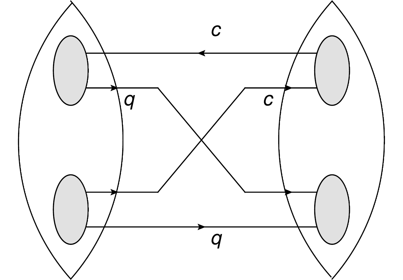
Figure 3. Mechanism of the mixing of Eqs. (1) and (3) schematically represented as a Feynman diagram.
-
1. The spectral densities for the
$ 0^{--} $ tetraquark state in Eq. (1):$ \rho^{\rm pert}(s)=\int_{\alpha_{\rm min}}^{\alpha_{\rm max}} {\rm d} \alpha \int_{\beta_{\rm min}}^{1-\alpha} {\rm d} \beta \bigg{\{}\frac{{\cal F}_{\alpha \beta}^{3}(\alpha+\beta-1)({\cal F}_{\alpha \beta}+m_Q^2(\alpha+\beta-1))}{2^{9}\pi^{6} \alpha^{3} \beta^{3}}\bigg{\}}\; , $

(A1) $ \rho^{\langle \bar{q} q\rangle}=0\;, $

(A2) $ \begin{aligned}[b] \rho^{\langle G^2 \rangle}(s) =\;&\frac{\langle G^2 \rangle}{2^{10}\pi^{6}} \int_{\alpha_{\rm min}}^{\alpha_{\rm max}} {\rm d} \alpha \int_{\beta_{\rm min}}^{1-\alpha} {\rm d} \beta \bigg{\{} \frac{- 3m_Q^2 {\cal F}_{\alpha \beta} }{ \alpha \beta} +\frac{\alpha+\beta-1}{2\alpha^3\beta^3} \Big( {\cal F}_{\alpha \beta} m_Q^2 \left(7 \alpha ^3+3 \alpha ^2 (\beta -1)+3 \alpha \beta ^2+(7 \beta -3) \beta ^2\right)\\ &+ m_Q^4 \left(\alpha ^4+\alpha ^3 (\beta -1)+\alpha \beta ^3+(\beta -1) \beta ^3\right) \Big)\bigg{\}}\;, \end{aligned} $

(A3) $ \rho^{\langle \bar{q} q\rangle^2}=\int_{\alpha_{\rm min}}^{\alpha_{\rm max}} {\rm d} \alpha \frac{3 \langle \bar{q} q\rangle^2(m_Q^2-{\cal H}_\alpha)}{8 \pi^{2}}\;, $

(A4) $ \rho^{\langle G^3 \rangle}(s) =\frac{\langle G^3 \rangle}{2^{11}\pi^{6}}\int_{\alpha_{\rm min}}^{\alpha_{\rm max}} \frac{{\rm d} \alpha}{ \alpha ^3} \int_{\beta_{\rm min}}^{1-\alpha} {\rm d} \beta (\alpha+\beta-1) \Big( 2{\cal F}_{\alpha \beta}+m_Q^2 (3\alpha +7\beta -3)\Big) \; , $

(A5) $ \rho^{\langle \bar{q} q\rangle\langle \bar{q} G q\rangle}=\int_{\alpha_{\rm min}}^{\alpha_{\rm max}} {\rm d} \alpha \frac{3\langle \bar{q} q\rangle\langle \bar{q} G q\rangle\alpha(\alpha-1)}{8 \pi^{2}}\;, $

(A6) $ \Pi^{\langle G^3 \rangle}(M_B^2)=\frac{m_Q^4\langle G^3 \rangle}{2^{11}\pi^6}\int_{0}^{1} \frac{{\rm d} \alpha}{ \alpha ^4} \int_{0}^{1-\alpha} {\rm d} \beta - (\alpha+\beta-1)^2\; {\rm e}^{-\frac{m_Q^2(\alpha+\beta)}{\alpha\beta M_B^2}}\;, $

(A7) $ \Pi^{\langle \bar{q} q\rangle\langle \bar{q} G q\rangle}(M_B^2)=\frac{m_Q^2\langle \bar{q} q\rangle\langle \bar{q} G q\rangle}{2^4\pi^2}\int_{0}^{1} {\rm d} \alpha \; {\rm e}^{-\frac{m_Q^2}{\alpha(1-\alpha) M_B^2}}\;\bigg{\{} \frac{3 m_Q^2}{\alpha(\alpha-1)M_B^2}-6 \bigg{\}} \;, $

(A8) where
$ M_B $ is the Borel parameter introduced by the Borel transformation, and$ Q = c $ or b. Here, we also have the following definitions:$ {\cal F}_{\alpha \beta} = (\alpha + \beta) m_Q^2 - \alpha \beta s \; , {\cal H}_\alpha = m_Q^2 - \alpha (1 - \alpha) s \; , $

(A9) $ \alpha_{\min} = \left(1 - \sqrt{1 - 4 m_Q^2/s} \right) / 2, \; , \alpha_{\max} = \left(1 + \sqrt{1 - 4 m_Q^2 / s} \right) / 2 \; , $

(A10) $ \beta_{\min} = \alpha m_Q^2 /(s \alpha - m_Q^2). $

(A11) 2. Spectral densities for the
$ 0^{--} $ tetraquark state in Eq. (2):$ \rho^{\rm pert}(s)=\int_{\alpha_{\min}}^{\alpha_{\max}} {\rm d} \alpha \int_{\beta_{\min}}^{1-\alpha} {\rm d} \beta \bigg{\{}\frac{3{\cal F}_{\alpha \beta}^{3}(\alpha+\beta-1)({\cal F}_{\alpha \beta}-m_Q^2(\alpha+\beta-1))}{2^{9}\pi^{6} \alpha^{3} \beta^{3}}\bigg{\}}\; , $

(A12) $ \rho^{\langle \bar{q} q\rangle}=0\;, $

(A13) $ \begin{aligned}[b] \rho^{\langle G^2 \rangle}(s) =\;&\frac{\langle G^2 \rangle}{2^{10}\pi^{6}} \int_{\alpha_{\min}}^{\alpha_{\max}} {\rm d} \alpha \int_{\beta_{\min}}^{1-\alpha} {\rm d} \beta \bigg{\{} \frac{ 3m_Q^2 {\cal F}_{\alpha \beta} }{ \alpha \beta} +\frac{\alpha+\beta-1}{2\alpha^3\beta^3} \Big( {\cal F}_{\alpha \beta} m_Q^2 \left( \alpha ^3-3 \alpha ^2 (\beta -1)-3 \alpha \beta ^2+( \beta+3) \beta ^2\right)\\ &- m_Q^4 \left(\alpha ^4+\alpha ^3 (\beta -1)+\alpha \beta ^3+(\beta -1) \beta ^3\right) \Big)\bigg{\}}\;, \end{aligned} $

(A14) $ \rho^{\langle \bar{q} q\rangle^2}=\int_{\alpha_{\min}}^{\alpha_{\max}} {\rm d} \alpha \frac{ \langle \bar{q} q\rangle^2(m_Q^2+3{\cal H}_\alpha)}{8 \pi^{2}}\;, $

(A15) $ \rho^{\langle G^3 \rangle}(s) =\frac{\langle G^3 \rangle}{2^{11}\pi^{6}}\int_{\alpha_{\min}}^{\alpha_{\max}} \frac{{\rm d} \alpha}{ \alpha ^3} \int_{\beta_{\min}}^{1-\alpha} {\rm d} \beta (\alpha+\beta-1) \Big( 2{\cal F}_{\alpha \beta}+m_Q^2 (\alpha -3\beta +3)\Big) \; , $

(A16) $ \rho^{\langle \bar{q} q\rangle\langle \bar{q} G q\rangle}=\int_{\alpha_{\min}}^{\alpha_{\max}} {\rm d} \alpha \frac{3\langle \bar{q} q\rangle\langle \bar{q} G q\rangle\alpha(1-\alpha)}{8 \pi^{2}}\;, $

(A17) $ \Pi^{\langle G^3 \rangle}(M_B^2)=\frac{m_Q^4\langle G^3 \rangle}{2^{11}\pi^6}\int_{0}^{1} \frac{{\rm d} \alpha}{ \alpha ^4} \int_{0}^{1-\alpha} {\rm d} \beta (\alpha+\beta-1)^2\; {\rm e}^{-\frac{m_Q^2(\alpha+\beta)}{\alpha\beta M_B^2}}\;, $

(A18) $ \Pi^{\langle \bar{q} q\rangle\langle \bar{q} G q\rangle}(M_B^2)=\frac{m_Q^2\langle \bar{q} q\rangle\langle \bar{q} G q\rangle}{2^4\pi^2}\int_{0}^{1} {\rm d} \alpha \; {\rm e}^{-\frac{m_Q^2}{\alpha(1-\alpha) M_B^2}}\;\bigg{\{} \frac{ m_Q^2}{\alpha(\alpha-1)M_B^2}+2 \bigg{\}} \;. $

(A19) 3. Spectral densities for the
$ 0^{--} $ tetraquark state in Eq. (3):$ \rho^{\rm pert}(s)=\int_{\alpha_{\min}}^{\alpha_{\max}} {\rm d} \alpha \int_{\beta_{\min}}^{1-\alpha} {\rm d} \beta \frac{3{\cal F}_{\alpha \beta}^{4}(\alpha+\beta-1)}{2^{9}\pi^{6} \alpha^{3} \beta^{3}}\; , $

(A20) $ \rho^{\langle \bar{q} q\rangle}=0\;, $

(A21) $ \rho^{\langle G^2 \rangle}(s)=\frac{m_Q^2\langle G^2 \rangle}{2^{9}\pi^{6}} \int_{\alpha_{\min}}^{\alpha_{\max}} \frac{{\rm d} \alpha}{\alpha^3} \int_{\beta_{\min}}^{1-\alpha} \frac{{\rm d} \beta}{\beta^3} {\cal F}_{\alpha \beta}(\alpha+\beta-1)(\alpha^3+\beta^3) \;, $

(A22) $ \rho^{\langle \bar{q} q\rangle^2}=\int_{\alpha_{\min}}^{\alpha_{\max}} {\rm d} \alpha \frac{ m_Q^2 \langle \bar{q} q\rangle^2}{4 \pi^{2}}\;, $

(A23) $ \rho^{\langle G^3 \rangle}(s) =\frac{\langle G^3 \rangle}{2^{10}\pi^{6}}\int_{\alpha_{\min}}^{\alpha_{\max}} \frac{{\rm d} \alpha}{ \alpha ^3} \int_{\beta_{min}}^{1-\alpha} {\rm d} \beta (\alpha+\beta-1) \Big( {\cal F}_{\alpha \beta}+2\beta m_Q^2 \Big) \; , $

(A24) $ \rho^{\langle \bar{q} q\rangle\langle \bar{q} G q\rangle}=0\;, $

(A25) $ \Pi^{\langle \bar{q} q\rangle\langle \bar{q} G q\rangle}(M_B^2)=\frac{m_Q^2\langle \bar{q} q\rangle\langle \bar{q} G q\rangle}{2^3\pi^2}\int_{0}^{1} {\rm d} \alpha \; {\rm e}^{-\frac{m_Q^2}{\alpha(1-\alpha) M_B^2}}\;\bigg{\{} \frac{ m_Q^2}{\alpha(\alpha-1)M_B^2}-1 \bigg{\}} \;. $

(A26) 4. Spectral densities for the
$ 0^{--} $ tetraquark state in Eq. (4):$ \rho^{\rm pert}(s)=\int_{\alpha_{\min}}^{\alpha_{\max}} {\rm d} \alpha \int_{\beta_{\min}}^{1-\alpha} {\rm d} \beta \frac{3{\cal F}_{\alpha \beta}^{4}(\alpha+\beta-1)}{2^{11}\pi^{6} \alpha^{3} \beta^{3}}\; , $

(A27) $ \rho^{\langle \bar{q} q\rangle}=0\;, $

(A28) $ \rho^{\langle G^2 \rangle}(s) =\frac{\langle G^2 \rangle}{2^{12}\pi^{6}} \int_{\alpha_{\min}}^{\alpha_{\max}} \frac{{\rm d} \alpha}{\alpha^3} \int_{\beta_{\min}}^{1-\alpha} \frac{{\rm d} \beta}{\beta^3} 2 m_Q^2{\cal F}_{\alpha \beta}(\alpha+\beta-1)(\alpha^3+\beta^3)-3{\cal F}_{\alpha \beta}^2\alpha\beta(\alpha+\beta) \;, $

(A29) $ \rho^{\langle \bar{q} q\rangle^2}=\int_{\alpha_{\min}}^{\alpha_{\max}} {\rm d} \alpha \frac{ m_Q^2 \langle \bar{q} q\rangle^2}{16 \pi^{2}}\;, $

(A30) $ \rho^{\langle G^3 \rangle}(s) =\frac{\langle G^3 \rangle}{2^{12}\pi^{6}}\int_{\alpha_{\min}}^{\alpha_{\max}} \frac{{\rm d} \alpha}{ \alpha ^3} \int_{\beta_{\min}}^{1-\alpha} {\rm d} \beta (\alpha+\beta-1) \Big( {\cal F}_{\alpha \beta}+2\beta m_Q^2 \Big) \; , $

(A31) $ \rho^{\langle \bar{q} q\rangle\langle \bar{q} G q\rangle}=0\;, $

(A32) $ \Pi^{\langle \bar{q} q\rangle\langle \bar{q} G q\rangle}(M_B^2)=\frac{m_Q^2\langle \bar{q} q\rangle\langle \bar{q} G q\rangle}{2^5\pi^2}\int_{0}^{1} {\rm d} \alpha \; {\rm e}^{-\frac{m_Q^2}{\alpha(1-\alpha) M_B^2}}\;\bigg{\{} \frac{ m_Q^2}{\alpha(\alpha-1)M_B^2}-1 \bigg{\}} \;. $

(A33) -
For the hidden-charm and hidden-bottom
$ 0^{--} $ tetraquark states in Eqs. (1)−(4), the OPE, pole contribution, and masses as functions of Borel parameter$ M_B^2 $ are given in Figs. B1 to B7.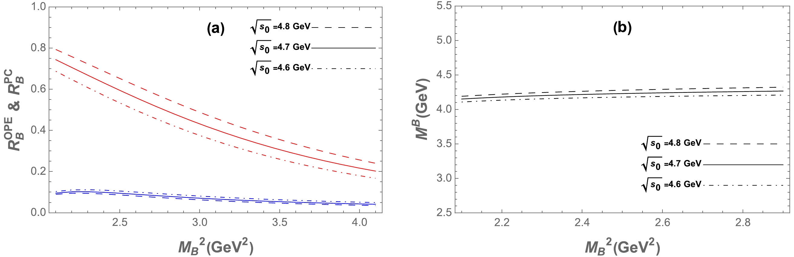
Figure B1. (color online) Same as in Fig. 2 but for the current in Eq. (2).
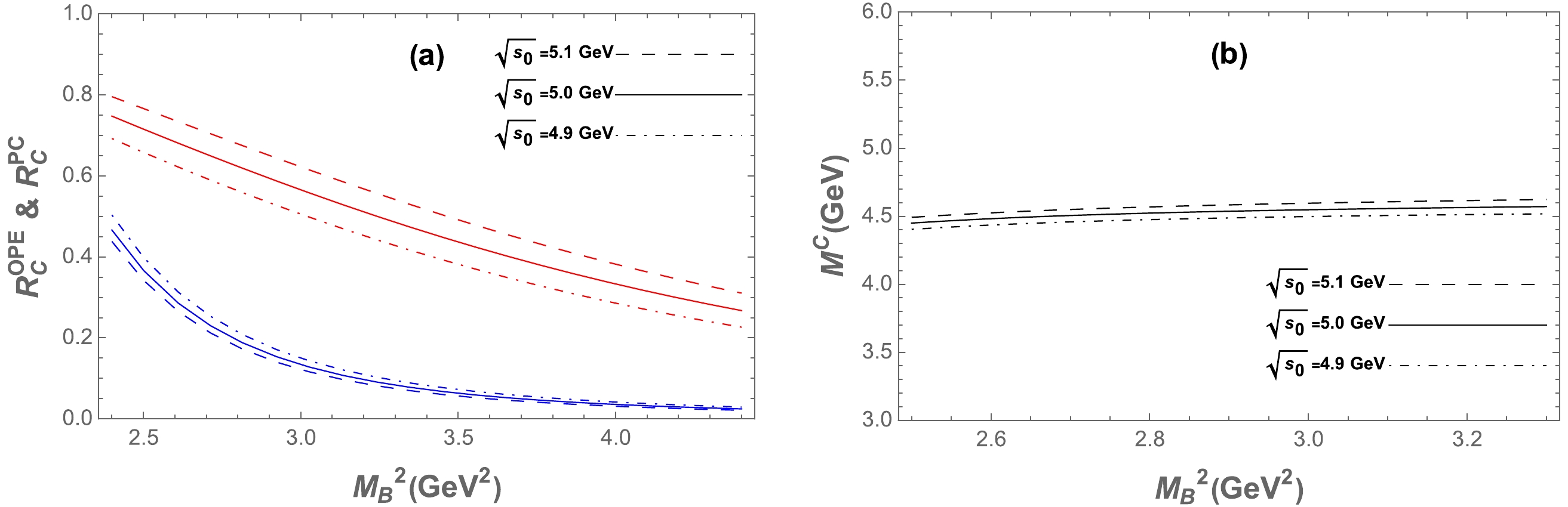
Figure B2. (color online) Same as in Fig. 2 but for the current in Eq. (3).
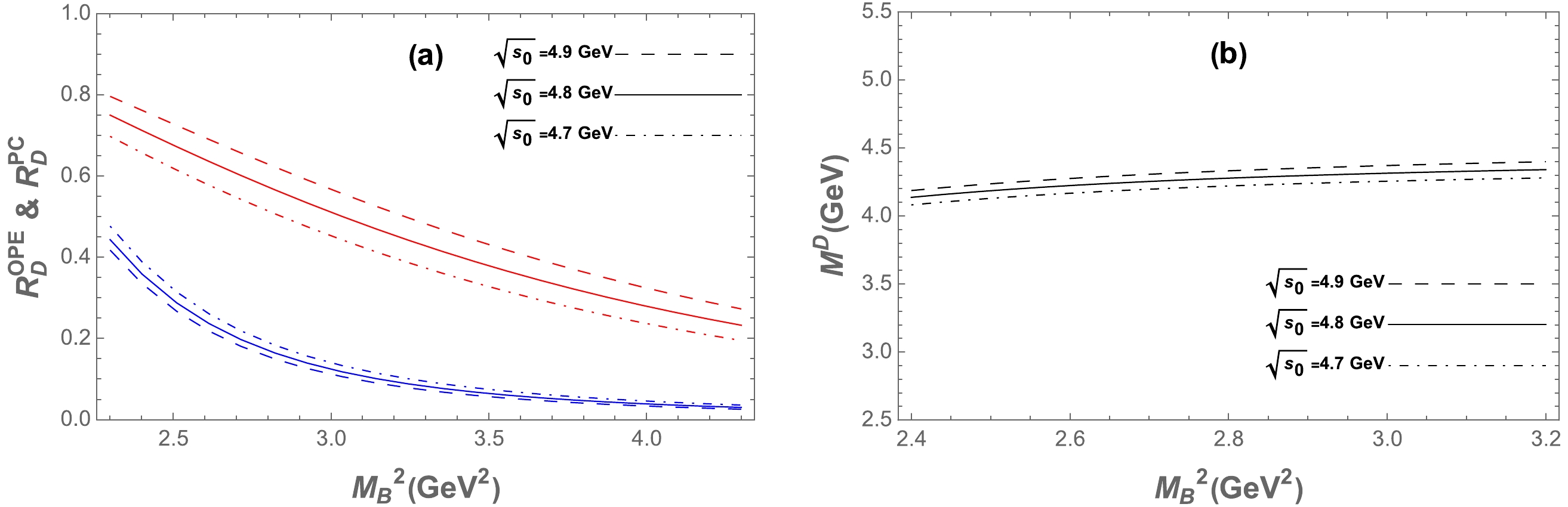
Figure B3. (color online) Same as in Fig. 2 but for the current in Eq. (4).
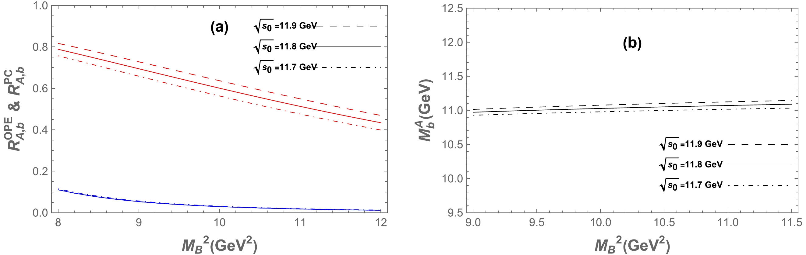
Figure B4. (color online) Same as in Fig. 2 but for the
$ 0^{--} $ hidden-bottom tetraquark state.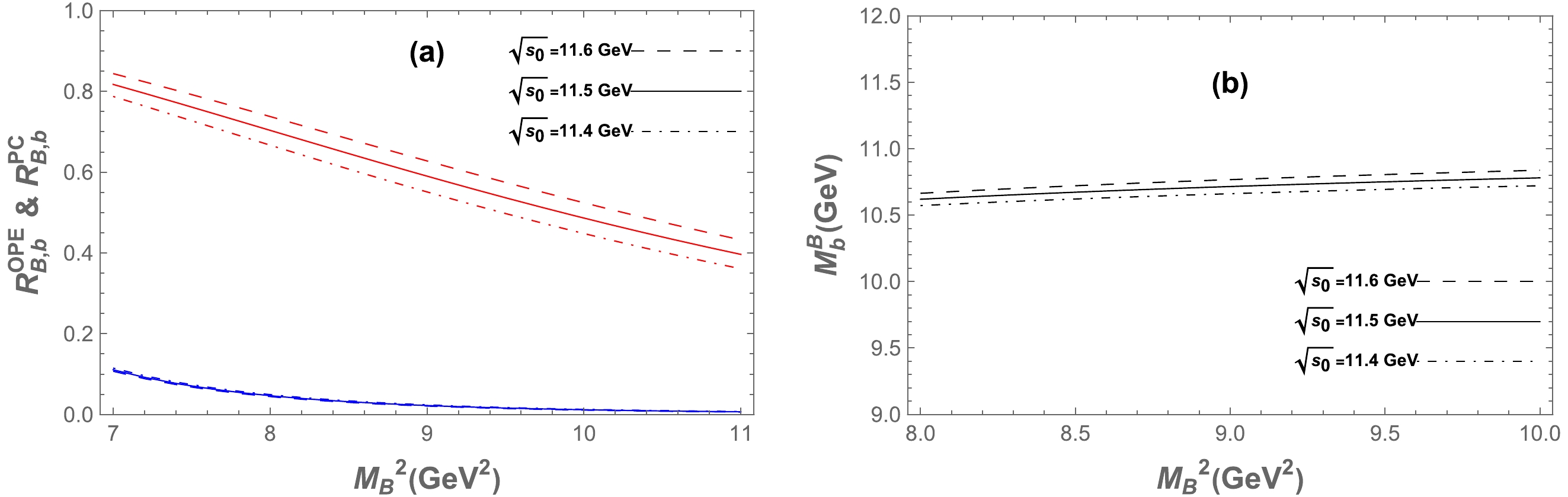
Figure B5. (color online) Same as in Fig. 2 but for the
$ 0^{--} $ hidden-bottom tetraquark state for the current in Eq. (2).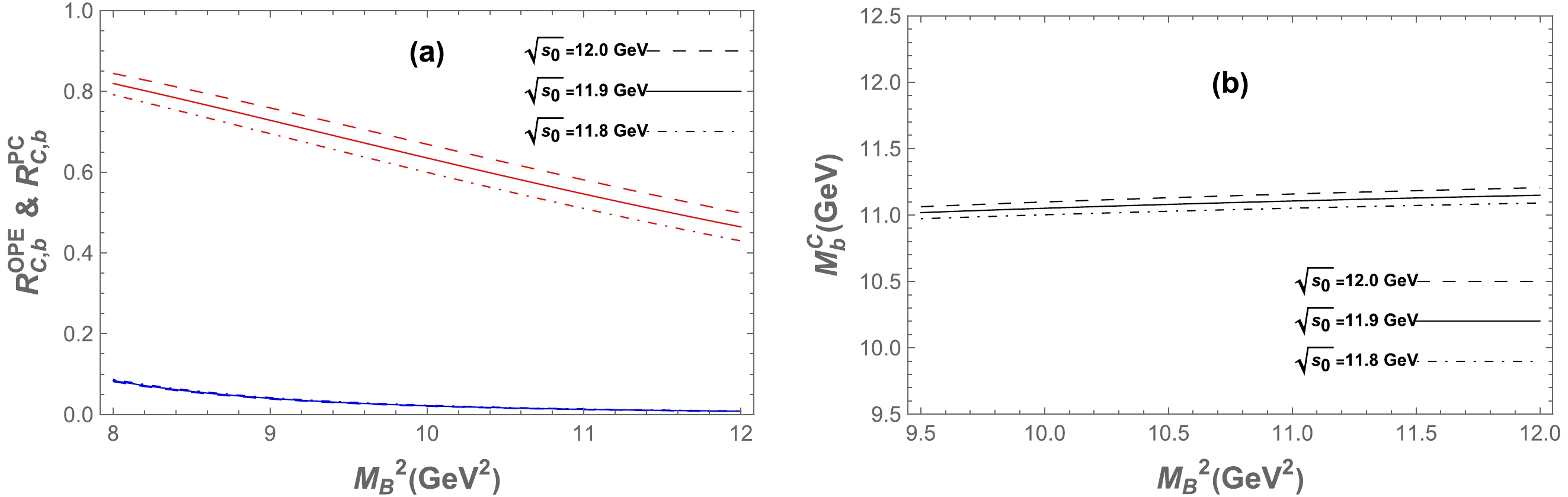
Figure B6. (color online) Same as in Fig. 2 but for the
$ 0^{--} $ hidden-bottom tetraquark state for the current in Eq. (3).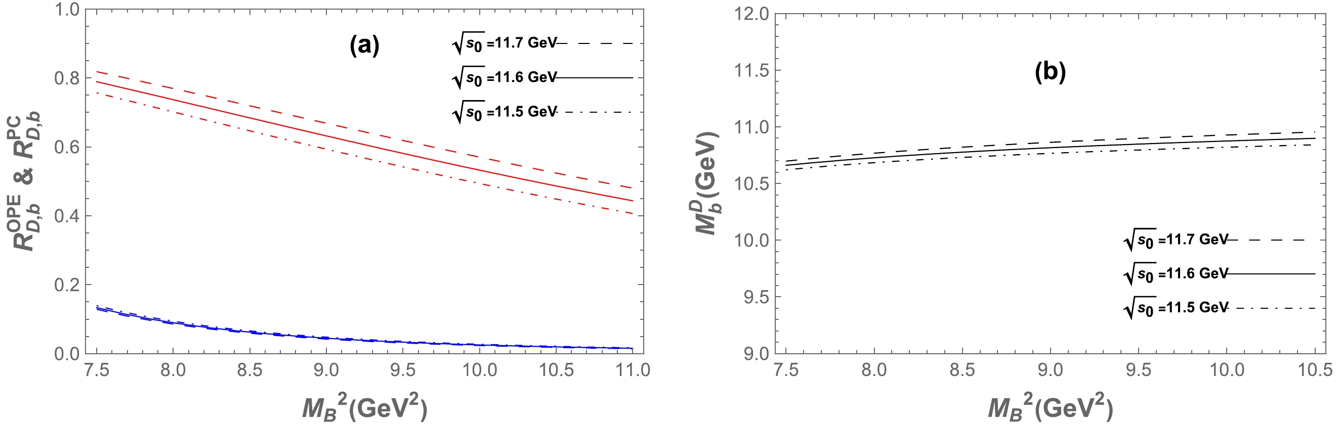
Figure B7. (color online) Same as in Fig. 2 but for the
$ 0^{--} $ hidden-bottom tetraquark state for the current in Eq. (4).
0– – hidden-heavy tetraquark states via QCD sum rules
- Received Date: 2024-03-11
- Available Online: 2024-09-15
Abstract: In this study, we evaluated the mass spectra of the prospective


 DownLoad: