


 Abstract
 HTML
HTML Reference
 Related
 PDF
PDF


-
In 1925, Edwin Hubble, an American astronomer, made the groundbreaking discovery that the universe is expanding. The universe was incredibly hot and dense after the Big Bang. The universe has continued to evolve and cool down, and most galaxies have moved away from the Milky Way. The universe is expanding so rapidly that it is experiencing an accelerating phase. The sustained acceleration of the universe's expansion in the long term is attributed to an exotic variable known for its negative pressure, commonly termed as dark energy (DE). It is defined by a tropical equation of state (EoS) in the form [1]
$ \omega=\frac{P}{\rho}, $

where P and ρ represent pressure and density, while ω is the equation of the state parameter. To consider candidates for DE, various DE models have been implemented, including the cosmological constant [2], quintessence [3], K-essence [4], CDM [5], Tachyon [6], Chaplygin gas (CG) [7], and holographic DE. The existence of the dark sector, which includes DE and dark matter (DM), remains unclear. To explain cosmic acceleration, a key candidate is DE with negative pressure.
The entire universe comprises 26.8% DM, 68.3% DE, and 4.9% ordinary (visible) matter. Big Bang cosmology is an essential tool for studying the expansion and characteristics of the universe. However, it falls short in explaining the origin of the large scale structure (LSS) of the universe and the formation of galaxies. In the context established by these problems, Guth proposed the inflationary theory, which provides a compelling solution to the horizon and flatness issues of the Big Bang model. It also offers a mechanism for describing the homogeneities of the early universe. Inflation is defined as the exponential expansion of the universe over time. After inflation, the universe transitions to a radiation-dominated era, where radiation gives way to matter and eventually, matter gives way to DE. The inflationary theory provides a solution to two fundamental problems of the early universe. The first problem arises from the assumption that the early universe was considered to be homogeneous (horizon problem) [8]. The second problem is the flatness problem, which suggests that the energy density of the present universe is very close to the critical value and depends on the shape of the universe (closed or open). Inflation can be divided into two categories: cold and warm.
Cold inflation represents the initial stage of inflation and has two phases, namely slow-roll and reheating era [9]. During the slow-roll phase, the universe expands, and after this expansion, a reheating period is required. This period allows the universe to transition into the radiation era, fulfilling the requirements of the Big Bang theory. Dissipation is a crucial factor in any physical system that interacts with its environment; however, cold inflation often neglects this effect. At the end of inflation, reheating becomes necessary to align with the radiation-dominated rule of the Big Bang. By contrast, warm inflation has the important feature of preventing the reheating process, because it involves the decay of inflation into radiation during the slow-roll phase at the end of accelerated expansion [10, 11]. Warm inflation exhibits different consistency relations compared to cases where dissipative effects are negligible, as in cold inflation. During the dissipation process, we can determine how the density of the vacuum inflation field changes into radiation, causing the universe to transition from an accelerated expansion phase to a radiation-dominated era [12].
The swampland criteria or conjectures [13, 14] can also be used to reconstruct the K-essence model. The swampland theory is a theory that does not satisfy the principles of string theory or Einstein's theory of gravity. The first conjecture states that the field of inflation is equal to the Planck mass, i.e.,
$ \triangle\phi\leq m_{p} $ , sometimes expressed as$ \triangle\phi\leq cm_{p} $ , where the value of c depends on the nature of the field. The second conjecture is related to the slope of the potential of the scalar field and is given by$ V_{\phi}\geq\dfrac{c}{m_p} $ , where$V_{\phi}=\dfrac{{\rm d}V}{{\rm d}\phi}$ . If these conjectures are true, then inflation may not occur, or it may occur on a small scale, depending on the value of c. We can also relate the second swampland conjecture to slow-roll parameters, which describe the slow variation of the scalar field ϕ over time and are expressed as$ \varepsilon = \frac{1}{2}\bigg(\frac{V_{\phi}}{V}\bigg)^{2},\quad \eta=\frac{V{_\phi{_\phi}}}{V}, $

(1) where
$ {V{_\phi}{_\phi}} $ represents second derivative with respect to (w.r.t) ϕ. Inflation takes place if$ \eta\ll1 $ and$ \varepsilon\ll1 $ .The concept of CG [15] initially emerged outside the realm of cosmology, yet its intriguing property of negative pressure has garnered renewed interest within the field. When integrated with the FLRW background in general relativity, this model elucidates the historical expansion of the cosmos in a universe filled with an unconventional fluid. Notably, CG models, distinguished by its non-constant EoS parameter, present several compelling features [16, 17]. Indeed, CG models have garnered attention in recent studies within the framework of modified gravity theories [18]. However, challenges arise in the formulation of structures and cosmological power spectra within the CG model [19]. Recently, Bento et al. [20] introduced the generalized Chaplygin gas (GCG) model as a solution to address or alleviate the challenges associated with the CG regarding dark energy. Extensive research has been conducted on the GCG model, aiming to elucidate the phenomenon of accelerating universe. Observational evidence has supported its validity [21–24]. One notable aspect of the GCG model is its capability to describe both dark matter and dark energy within a unified fluid framework, facilitated by an exotic equation of state [25].
This manuscript is organized as follows:
● In Sec. II, we provide a concise overview of the warm inflationary scenario and cosmological perturbations.
● Basic formulations of CG and GCG are provided in Sec. III.
● In Sec. IV, we analyze the quasi-exponential potential, examining inflationary parameters and exploring swampland conjectures associated with the underlying potential. Additionally, we present graphical representations illustrating the behavior of these parameters and conjectures, offering insights into the dynamics of the quasi-exponential inflationary scenario.
● Mixed large field inflation is discussed in Sec. V. We derive expressions and graphically check the behavior of some crucial inflationary parameters as well as swampland conjectures.
● In Sec. VI, we assume an exponential form of single-field inflation and investigate the underlying inflationary parameters and conjectures.
● In the concluding Sec. VII, we present and discuss findings derived from our exploration of various inflationary scenarios, potential forms, and associated parameters and conjectures. This section includes a comprehensive summary and interpretation of the results, offering a conclusive perspective on the implications of our study.
● In Sec. VIII, long calculations derived from our study are presented.
-
We begin with the expression of the Friedmann equation applicable to a flat Friedmann-Robertson-Walker (FRW) universe, taking into account the existence of a conventional scalar field alongside a radiation fluid. The equation is outlined as follows:
$ H^2=\frac{1}{3M_P^2}(\rho_\phi+\rho_\gamma), $

(2) where
$M_P=({\sqrt{8\pi G}})^{-1}$ expresses the reduced Planck mass and G denotes the gravitational constant. Here,$ \rho_\gamma $ is the energy density of radiation while$ \rho_\phi $ denotes the energy density of a standard scalar field such that$\rho_\phi= \dot{\phi}^2 /{2} +V(\phi)$ (where$\dot{\phi}=\dfrac{{\rm d}\phi}{{\rm d}t}$ ). For both scalar fields, the corresponding conservation equations become$ \dot{\rho}_\phi+3H(P_{\phi}+\rho_{\phi}) = -\Gamma\dot{\phi}^{2}, $

(3) $ \dot{\rho}_\gamma+4H\rho_{\gamma} = \Gamma\dot{\phi}^{2}, $

(4) where
$ \Gamma>0 $ and$ P_\phi=\dfrac{\dot{\phi}^2}{2}- V(\phi) $ expresses the pressure of the scalar field. Substituting the expressions for energy densities of both the scalar field and radiation into the first conservation equation, we obtain$ \ddot{\phi}+(3H+\Gamma)\dot{\phi}+V'(\phi)=0, $

(5) where
$ V'=\dfrac{{\rm d}V}{{\rm d}\phi} $ . Additionally, the term$ \Gamma\dot{\phi} $ signifies the interaction between the scalar field and radiation, where Γ dictates the decay of the scalar field into radiation. The decay rate of the inflaton may depend on the scalar field alone, the temperature of the thermal bath, or a combination of both quantities; it may also even be a constant.In the context of warm inflation, the generation of radiation remains quasi-stable, i.e.,
$ \dot{\rho}_{\gamma}\ll4H\rho_{\gamma} $ and$\dot{\rho}_{\gamma}\ll \Gamma\dot{\phi^{2}}$ , as derived in [26, 27]. Therefore, under the slow-roll approximation, the equations of motion can be expressed as$ -3H\dot{\phi}(1+R) \simeq V_{\phi}, $

(6) $ 4H\rho_{\gamma} \simeq \Gamma\dot{\phi^{2}}. $

(7) Here, R expresses the dissipative ratio:
$ R\equiv\frac{\Gamma}{3H}. $

(8) Normally, during the evaluation of warm inflation, two types of regimes occur: strong dissipative regime, where
$ R\gg1 $ , and weak regime, in which$ R\ll1 $ [28]. By considering thermalization, the energy density of the radiation field is expressed as$ \rho_{\gamma}= C_{\gamma}T^{4} $ , where$C_{\gamma}={\pi^{2}g_{*}}/{30}$ and$ g_{*} $ represents the number of relativistic degree of freedom. Using Eqs. (6) and (7) with$ \rho_\gamma\propto T^4 $ , we obtain the temperature of the thermal bath:$ T=\bigg[\frac{\Gamma V^{2}_{,{\phi}}}{36C_\gamma\; H^{3}(1+R)^{2}}\bigg]^{\frac{1}{4}}. $

(9) Typically, inflation occurs when the set of slow-roll conditions is satisfied. In warm inflation, the slow-roll parameters are defined as [29]
$ \begin{aligned}[b]& \epsilon = \frac{1}{2}\bigg(\frac{V_,{_\phi}}{V}\bigg)^{2},\quad \eta=\bigg(\frac{V_,{_\phi{_\phi}}}{V}\bigg),\\ &\beta = \bigg(\frac{\Gamma_,{_\phi}V_,{_\phi}}{\Gamma V}\bigg),\quad\sigma=\bigg(\frac{V_,{_\phi}}{\phi V}\bigg). \end{aligned} $

(10) The conditions for slow-roll in warm inflation can be formulated as
$ \epsilon\ll R+1,\quad \eta\ll R+1, \quad \beta\ll R+1,\quad \sigma\ll R+1. $

When one of these conditions is no longer fulfilled, either the expansion's movement is no longer over-damped and slow-roll ends, or the radiation becomes practically identical to the expansion energy density.
-
In the warm inflation model, where a thermalized radiation component coexists with
$ T>H $ , the fluctuations in inflation, denoted as$ \delta\phi $ , are primarily thermal rather than quantum. Consequently, the amplitude of the power spectrum of the curvature perturbation is determined by [30]$ {\cal{P}}_{{\cal{R}}}^\frac{1}{2}\simeq\bigg(\frac{H}{2\pi}\bigg)\bigg(\frac{3H^{2}}{V_,{_\phi}}\bigg) (1+R)^\frac{5}{4}\bigg(\frac{T}{H}\bigg)^\frac{1}{2}. $

(11) The normalization has been set to retrieve the conventional cold inflation outcome as
$ R\rightarrow0 $ and$ T\simeq H $ . Conversely, the scalar spectral index$ n_{s} $ , in the leading order of the slow-roll approximation, is expressed as [30]$ \begin{aligned}[b]n_{s} =\;& \frac{\rm d}{{\rm d}\ln k}(\ln P_{R})+1, \\ \simeq\;& 1-\frac{(17+9R)}{4(1+R)^{2}}\epsilon-\frac{(1+9R)}{4(1+R)^{2}}\beta+\frac{3}{2(1+R)}\eta.\end{aligned} $

(12) The expression for the running of the scalar spectral index, indicating the scale dependence of the spectral index, is provided by the equation for
${{\rm d}n_{s}}/{{\rm d}\ln{k}}$ presented in [29]:$ \frac{{\rm d}n_{s}}{{\rm d}\ln{k}}= \frac{1}{R^{2}}\bigg(-\frac{9 \beta^2}{2}+\frac{15\beta\eta}{4}-\frac{9\beta\epsilon}{2}+\frac {9 \gamma\epsilon}{2}-\frac{3\zeta^2}{2}-\frac{27\epsilon^2}{4}+6\eta \epsilon\bigg), $

(13) where
$ \zeta^{2} $ and γ (second-order slow-roll parameters) are defined as [31]$ \zeta^{2} = \bigg(\frac{V_{,} {_\phi}V_{,}{{_\phi}{_\phi}{_\phi}}}{V^{2}}\bigg),\quad \gamma=\bigg(\frac{\Gamma_{,}{_\phi}{_\phi}}{\Gamma}\bigg). $

(14) The tensor-to-scalar ratio r is expressed as [30]
$ r=\frac{16H\epsilon(1+R)^{-\frac{5}{2}}}{T}. $

(15) When examining a specific type of scalar potential and dissipative coefficient Γ, it is possible to concentrate on the background evolution by utilizing the slow-roll parameters. We investigate how an inflationary decay rate, characterized by a general power-law dependence on both the scalar field ϕ and temperature of the thermal bath T, influences the inflationary features for the power-law plateau potential. We restrict our analysis to the strong dissipation regime. Under the assumption that inflationary dynamics occur within the strong dissipative regime
$ (R\gg1) $ or$ (\Gamma\gg3H) $ , we employ a general parametrization of the dissipative coefficient$\Gamma(\phi, T) = C_\phi{T^{a}}/{\phi^{a-1}}$ (where$ C_{\phi} $ and a represent dimensionless parameters associated with the dissipative microscopic dynamics and inflation decay rate, respectively). For this choice, Eq. (9) becomes$ T = \bigg(\frac{V^2_{{,}\phi}\phi^{a-1}C^{-1}_{\phi}}{4C_{\gamma} H}\bigg)^\frac{1}{(4+a)}. $

(16) -
CG [15] is a theoretical model in physics and cosmology. It constitutes a unique form of exotic matter with distinct properties. Named after the Russian mathematician Sergei Chaplygin, this gas is characterized by its equation of state, which relates pressure and density in a non-trivial manner. The EoS of CG is expressed as
$p=-{C_1}/{\rho}$ , where$ C_1 $ is a positive constant while ρ and p denote the energy density and pressure, respectively. Unlike conventional gases, the CG equation of state incorporates both attractive and repulsive forces, making it a versatile candidate for explaining certain phenomena in astrophysics and cosmology. Originally proposed to model the lift force on an airfoil, the CG has found applications in various cosmological scenarios, including being a candidate for dark energy. Its ability to exhibit features of both attractive and repulsive gravity makes it a fascinating subject for theoretical research, with implications for understanding the fundamental nature of the universe.The GCG model [20] is an extension of the original CG designed to offer a more versatile and comprehensive framework for describing various cosmological scenarios. This model introduces additional parameters and features to enhance its ability to explain the dynamics of both dark matter and dark energy in the universe. The equation of state for GCG is expressed as
$p=-{C_1}/{\rho^\alpha}$ , where$ 0<\alpha\leq1 $ is a positive constant. Notably, when α equals 1, GCG reduces to the original CG, and different values of α result in diverse behaviors, ranging from quintessence-like to phantom-like properties. One can obtain the energy density of GCG through the conservation equation as follows:$ \rho=\left(C_1+\frac{C_2}{a^{3(1+\alpha)}}\right)^{\frac{1}{1+\alpha}}. $

(17) Here,
$ C_2 $ represents the constant of integration. In this context, the term proportional to$ a^{-3} $ corresponds to the energy density of matter$ \rho_m $ .Through an extrapolation of Eq. (17), the identification of the energy density of matter
$ \rho_m $ is extended to include the contribution from the energy density associated with the standard scalar field$ \rho_\phi $ , resulting in$ \rho=(C_1+\rho_m^{1+\alpha})^{\frac{1}{1+\alpha}}\rightarrow (C_1+\rho_\phi^{1+\alpha})^{\frac{1}{1+\alpha}}. $

(18) Referring to it as a non-covariant modification of gravity, we refrain from regarding Eq. (18) a consequence of Eq. (17). Instead, it is considered to give rise to a modified Friedmann equation, as highlighted in [22]. In a spatially flat universe featuring a self-interacting inflation field denoted as ϕ, alongside a radiation field, the Friedmann equation, that is, Eq. (2), can be expressed as
$ H^2=\frac{1}{3}((C_1+\rho_\phi^{1+\alpha})^{\frac{1}{1+\alpha}}+\rho_\gamma). $

(19) Here, we consider
$ M_p^2=1 $ .Emphasizing that Eq. (19) arises from a non-covariant modification of gravity, it is relevant, as highlighted in [23], that the effect leading to Eq. (19) can be assumed to preserve diffeomorphism invariance in (3+1) dimensions, thereby ensuring total stress-energy conservation. In the inflationary phase, dominance of the energy density of the scalar field over the energy density of the radiation field is observed. It is expressed as
$ \rho_\phi\gg\rho_\gamma $ , resulting in$ \rho_\phi\sim V $ . For simplicity, we adopt$ \alpha=1 $ . Consequently, the Friedmann equation expressed by Eq. (19) transforms into$ H^2=\frac{1}{3}\sqrt{C_{1}+V^2}. $

(20) Here, H denotes the Hubble parameter such that
$ H=\dfrac{\dot{a}}{a} $ and$\dot{a}=\dfrac{{\rm d}a}{{\rm d}t}$ .Note that inflationary parameters such as the power spectrum and scalar spectral index remain consistent within the framework of both the generalized Chaplygin gas model and the warm inflationary scenario, even when considering a standard scalar field coupled with radiation. Various authors used these observables for warm Chaplygin gas models in the context standard scalar field with radiation. In [32], the authors investigated the warm Chaplygin gas inflationary model within the framework of the effective field theory of loop quantum cosmology. They examined the primordial perturbation spectra, tensor-to-scalar ratio, and spectral indices for the underlying model during the slow-roll phase of inflation. Similarly, Campo and Herrera [33] discussed warm inflationary universe models in the context of a Chaplygin gas equation. They considered the chaotic potential and found various inflationary parameters. Furthermore, in [34], an intermediate inflationary model was explored within the framework of a generalized Chaplygin gas. The authors investigated the conditions of an inflationary epoch by using a standard scalar field and a tachyon field. Furthermore, in [35], the authors studied warm intermediate inflationary universe models in the presence of a generalized Chaplygin gas. In this paper, we examine the dynamics of inflation by employing the slow-roll approximations within both weak and strong dissipative regimes.
-
The Hamilton-Jacobi approach, described in [36], provides a robust method for examining single-field inflation. This approach allows for recasting the equations of motion with the inflaton, rather than the cosmic time, as the independent variable. It can be applied whenever the scalar field undergoes a continuous evolution over time. Unlike the inflaton potential, which is specific to the scalar field, the Hubble parameter is a geometric property. Therefore, it is more natural to describe inflation in terms of
$ H(\phi) $ rather than$ V(\phi) $ . For example,$ H(f)\sim \exp(\phi) $ corresponds to power-law inflation [37]. Moreover, the Planck collaboration has adopted this formalism to reconstruct the inflaton potential beyond the limitations of the slow-roll approximation. In [38], the authors derived a quasi-exponential inflaton potential using the Hamilton-Jacobi approach, which is presented as$ V(\phi)=\frac{3H_{\rm inf}^2}{8\pi} {\rm e}^{\frac{2\phi}{p(\phi+1)}}, $

(21) where
$H_{\rm inf}$ and p are the free parameters. This potential possesses a notable characteristic, as it effectively resolves the exit problem from inflation when compared to the widely recognized power-law potential. However, it is important to note that the resulting inflaton potential lacks a minimum point, which prompts the question of how to handle the reheating challenge within this model. Nonetheless, it is suggested that the warm inflation scenario could provide a potential solution to this issue. Combining Eqs. (20) and (21) with Eq. (16), the temperature of the thermal bath as a function of the inflation field ϕ becomes$\begin{aligned}\\[-8pt] T=\frac{5}{9^{(4+a)}}256^{-(4+a)^{-1}}\pi^{\frac{-2}{4+a}}\left(\frac{{\rm e}^{\frac{4\phi}{p(1+\phi)}} H^{4}_{\rm inf}\phi^{-1+a}\Bigg(\dfrac{2}{p(1+\phi)}-{\dfrac{2\phi}{P(1+\phi)^2}}\Bigg)^2}{C_\phi C_\gamma\Bigg(\dfrac{9 {\rm e}^{\frac{4\phi}{p(1+\phi)}}H^{4}_{\rm inf}}{64\pi^{2}}+C_1\Bigg)^\frac{1}{4}}\right)^{{1}/({4+a})}.\\ \end{aligned}$ 
(22) Using this value of T in expression
$ \Gamma(\phi_,T)=C_\phi\dfrac{T^{a}}{\phi^{a-1}} $ , the inflation decay rate becomes$ \Gamma = \left[\left(\frac{\phi^{a-1} H_{\inf }^4 {\rm e}^{\frac{4 \phi }{p (\phi +1)}} \left(\dfrac{2}{p (\phi +1)}-\dfrac{2 \phi }{p (\phi +1)^2}\right)^2}{C_{\gamma } C_{\phi } \sqrt[4]{C_1+\dfrac{9 H_{\inf }^4 {\rm e}^{\frac{4 \phi }{p (\phi +1)}}}{64 \pi ^2}}}\right)^{{1}/({a+4})} \times 3^{\frac{5}{2 (a+4)}} 256^{-\frac{1}{a+4}} \pi ^{-\frac{2}{a+4}} \right]^a \phi^{1-a}C_{\phi}. $

(23) For this expression of Γ, the dissipative ratio from Eq. (8) yields
$ R = \frac{\left[3^{\frac{5}{2 (a+4)}}256^{-\frac{1}{a+4}} \pi ^{-\frac{2}{a+4}} \left(\dfrac{\phi^{a-1} H_{\inf }^4 {\rm e}^{\frac{4 \phi }{p (\phi +1)}} \left(\dfrac{2}{p (\phi +1)}-\dfrac{2 \phi }{p (\phi +1)^2} \right)^2}{C_{\gamma } C_{\phi } \sqrt[4]{C_1+ \dfrac{9 H_{\inf }^4 {\rm e}^{\frac{4 \phi }{p (\phi +1)}}}{64 \pi ^2}}}\right)^{{1}/({a+4})}\right]^a}{\sqrt{3} \sqrt[4]{C_1+\dfrac{9 H_{\inf }^4 {\rm e}^{\frac{4 \phi }{p (\phi +1)}}}{64\pi ^2}}} \times \phi ^{1-a} C_{\phi}.$

(24) Concerning the underlying potential, the set of slow-roll parameters can be found as described in Appendix 8.1. For
$ R\gg 1 $ , the slow-roll conditions are$ \epsilon\ll R,\quad \eta\ll R, \quad \beta\ll R,\quad \sigma\ll R. $

(25) -
Here, we discuss the behavior of cosmological perturbations in strong dissipative regime
$R={\Gamma}/{(3H)} > 1$ . Forthis regime, the amplitude of the scalar power spectrum from Eq. (11) becomes$ {\cal{P}}_{{\cal{R}}}^{{1}/{2}}\simeq\bigg(\frac{H}{2\pi}\bigg)\bigg(\frac{3H^{2}}{V_{\phi}}\bigg) \bigg(\frac{T}{H}\bigg)^{{1}/{2}}R^{{5}/{4}}. $

(26) Using all the relevant expression, Eq. (26) becomes
$ \begin{aligned}[b]&{\cal{P}}_{{\cal{R}}} = \frac{3^{\frac{-(13a+32)}{4(a+4)}} 4^{\frac{2a}{a+4}} }{H_{\inf }^4 \Bigg(\dfrac{2}{p (\phi +1)}-\dfrac{2 \phi }{p (\phi +1)^2}\Bigg)^2} \left(\frac{\phi^{a-1} H_{\inf }^4 {\rm e}^{\frac{4 \phi }{p (\phi +1)}} \left(\dfrac{2}{p (\phi +1)}-\dfrac{2 \phi }{p (\phi +1)^2}\right)^2}{C_{\gamma } C_{\phi }\sqrt[4]{C_1+\dfrac{9 {H_{1}}^4 {\rm e}^{\frac{4 \phi }{p (\phi +1)}}}{64 \pi ^2}}}\right)^{{2}/({a+4})}\\&\times \left[\frac{\left( 3^{\frac{5}{2 (a+4)}} 256^{-\frac{1}{a+4}} \pi ^{-\frac{2}{a+4}} \left( \frac{\displaystyle\phi^{a-1} H_{\inf }^4 {\rm e}^{\frac{4\phi }{p (\phi +1)}} \left(\dfrac{2} {p (\phi +1)}-\dfrac{2 \phi }{p (\phi +1)^2}\right)^2} {C_{\gamma } C_{\phi }\sqrt[4]{C_1+\dfrac{9H_{\inf}^4 {\rm e}^{\frac{4 \phi }{p (\phi +1)}}}{64 \pi ^2}}}\right)^{{1}/({a+4})} \right)^a}{\sqrt[4]{C_1+\dfrac{9 H_{\inf }^4 {\rm e}^{\frac{4 \phi }{p (\phi +1)}}}{64 \pi ^2}}} \phi ^{1-a} C_{\phi }\right]^{5/2} \Bigg( C_1 + \dfrac{9 H_{\inf }^4 {\rm e}^{\frac{4 \phi }{p (\phi +1)}}}{64 \pi ^2}\Bigg)\pi ^{-\frac{4}{a+4}}{\rm e}^{-\frac{4 \phi }{p (\phi +1)}}.\end{aligned} $ 
(27) For
$ R\gg1 $ , the scalar spectral index$ n_s $ is defined as$ n_s = 1+\frac{1}{R}(-9\epsilon-9\beta+6\eta). $

(28) Substituting Eqs. (24) and (25) into Eq. (28), we obtain the expression of scalar spectral index (Appendix A, Eq. (A3). In this scenario, the expressions of second-order slow-roll parameters (
$ (\zeta^{2}) $ and γ) are provided in Appendix A. The tensor-to-scalar ratio for underlying potential is determined by replacing Eqs. (20), (22), (24), and (25) into Eq. (15), yielding Eq.(A5) (Appendix A). Similarly, the expression of running scalar spectral index is given in Eq. (A6). -
The string theory landscape, or landscape of vacua, encompasses a collection of possible false vacua in string theory, along with a comprehensive 'landscape' of choices of parameters that control compactifications [39]. In general, the term 'swampland' indicates effective low-energy physical theories that are not consistent with string theory. The swampland conjectures constitute a set of speculated criteria for theories within the string theory landscape. To delineate the boundary separating the landscape from the swampland, two recent swampland conjectures have been proposed:
● Swampland distance conjecture:
The field-range traversed by the scalar fields in field space of the effective field theory (EFT) has an upper bound expressed as
$ \frac{\Delta\phi}{M_{p}}\leq C_{1}, $

where
$ C_{1} $ is a constant of order of unity.● Swampland de-Sitter conjecture:
The scalar field potentials of any EFT should obey one of the following conditions [40−46]:
$ \frac{|\Delta V|}{V}\geq \frac{C_{2}}{M_{p}}, $

$ \frac{\rm min(\nabla_{i}\nabla_{j}V)}{V}\leq - \frac{C_{3}}{M_{p}}, $

where
$ C_{2} $ and$ C_{3} $ are positive constants of order of unity;$ \nabla $ is gradient in field space, and${\rm min}(\nabla_{i}\nabla_{j}V)$ is the minimum eigenvalue of the Hessian$ \nabla_{i}\nabla_{j}V $ in an orthonormal frame.Ooguri et al. [41] reported a derivation of the de Sitter conjecture that merges the distance criterion with an entropy argument. The postulation posits that the entropy attributed to low mass bulk states within a Hubble volume cannot exceed the Gibbons-Hawking entropy [42]. This corresponds to a Boussos covariant entropy bound [43] adapted to a cosmological backdrop. In the scenario of warm inflation, an additional origin of bulk energy arises from the thermal states generated as a result of dissipative effects, wherein a portion of the inflaton's energy density is transformed. The dissipative effects during the slow-roll phase of warm inflation engender a thermal reservoir of light particles that interact with the inflaton [44]. In this study, our focus lies on examining the alteration of the de-Sitter conjecture by incorporating the additional entropy generated during a phase of warm inflation.
Considering that this additional entropy production could potentially impose a more stringent constraint on the slope of the potential, a thorough investigation is essential to ascertain whether the Bousso bound can still be upheld. In the above scenario, the term
${\dot{s}}/{(6\pi M_p^2\dot{H})}$ can also be expressed as [45]$ \frac{\dot{s}}{6\pi M_p^2\dot{H}}= \frac{s}{6\pi M_p^2H}\frac{s'H}{s H'}, $

where
$ ' $ denotes the derivative w.r.t ϕ and$ \dfrac{s'H}{s H'}=\dfrac{6T'V}{TV'} $ . It is suggested that if the ratio satisfies the condition${(T'V)}/{(V'T)} < 1$ , it meets the swampland conjectures [45]. Hence, following [45], we can identify the modified form of de-Sitter conjecture in warm inflationary scenario as$ \begin{aligned}[b]\\[-5pt] \dfrac{T'V}{V'T} =\;& \dfrac{\phi ^{1-a}C_{\gamma } C_{\phi } {\rm e}^{-\frac{4 \phi }{p (\phi +1)}}}{(a+4) H_{\inf }^4 \Bigg(\dfrac{2}{p (\phi +1)}-\dfrac{2 \phi }{p (\phi +1)^2}\Bigg)^3} \sqrt[4]{C_1+\dfrac{9 H_{\inf }^4 {\rm e}^{\frac{4 \phi }{p (\phi +1)}}}{64 \pi ^2}}\\&\times \left(\frac{2 \phi^{a-1} H_{\inf }^4 {\rm e}^{\frac{4 \phi }{p (\phi +1)}} \bigg(\dfrac{4 \phi }{p (\phi +1)^3}-\dfrac{4}{p (\phi +1)^2}\bigg) \bigg(\dfrac{2}{p (\phi +1)}-\dfrac{2 \phi }{p (\phi +1)^2}\bigg)}{C_{\gamma } C_{\phi } \sqrt[4]{C_1+\dfrac{9 H_{\inf }^4 {\rm e}^{\frac{4 \phi }{p (\phi +1)}}}{64 \pi ^2}}}\right)\\& + \frac{(a-1) \phi ^{a-2} H_{\inf }^4 {\rm e}^{\frac{4 \phi }{p (\phi +1)}} \bigg(\dfrac{2}{p (\phi +1)}-\dfrac{2 \phi }{p (\phi +1)^2}\bigg)^2}{C_{\gamma } C_{\phi } \sqrt[4]{C_1+\dfrac{9 H_{\inf }^4 {\rm e}^{\frac{4 \phi }{p (\phi +1)}}}{64 \pi^2}}}+\phi^{a-1} H_{\inf }^4 {\rm e}^{\frac{4 \phi }{p (\phi +1)}}\\& \times \frac{\bigg(\dfrac{2}{p (\phi +1)}-\dfrac{2 \phi }{p (\phi +1)^2} \bigg)^2 \bigg(\dfrac{4}{p (\phi +1)}-\dfrac{4 \phi }{p (\phi +1)^2}\bigg)}{C_{\gamma } C_{\phi } \sqrt[4]{C_1+\dfrac{9 H_{\inf }^4 {\rm e}^{\frac{4 \phi }{p (\phi +1)}}}{64 \pi ^2}}}-9 \phi^{a-1} H_{\inf }^8 {\rm e}^{\frac{8 \phi }{p (\phi +1)}}\\ \end{aligned} $ 
$ \begin{aligned}[b] &\times \left(\frac{\bigg(\dfrac{2}{p (\phi +1)}-\dfrac{2 \phi }{p (\phi +1)^2}\bigg)^2 \bigg(\dfrac{4}{p (\phi +1)}-\dfrac{4 \phi }{p (\phi +1)^2}\bigg)}{256 \pi ^2 C_{\gamma } C_{\phi } \bigg(C_1+\dfrac{9 H_{\inf }^4 {\rm e}^{\frac{4 \phi }{p (\phi +1)}}}{64 \pi ^2}\bigg)^{5/4}}\right). \end{aligned} $

-
In this section, we present plots of different inflationary parameters and swampland conjectures as functions of the scalar spectral index. The inflationary model undergoes testing and constraint evaluation by comparing it to contemporary astrophysical and cosmological observations, with a particular focus on data derived from temperature fluctuations in the cosmic microwave background (CMB). In practical terms, the predictions of various inflationary potential models are plotted on the
$ n_s - r $ plane. This plane also includes the contour plots depicting the regions permitted by the observed data. Recently, the Planck collaboration has released a set of more accurate data related to the anisotropies in the CMB temperature [47, 48]. Hence, we check the behavior of r versus$ n_{s} $ , R versus$ n_{s} $ ,$\dfrac{{\rm d}n_{s}}{{\rm d}\ln k}$ versus$ n_{s} $ , and$ {\dfrac{\acute{T} V}{T \acute{V}}} $ versus$ n_{s} $ .● Behavior of r versus
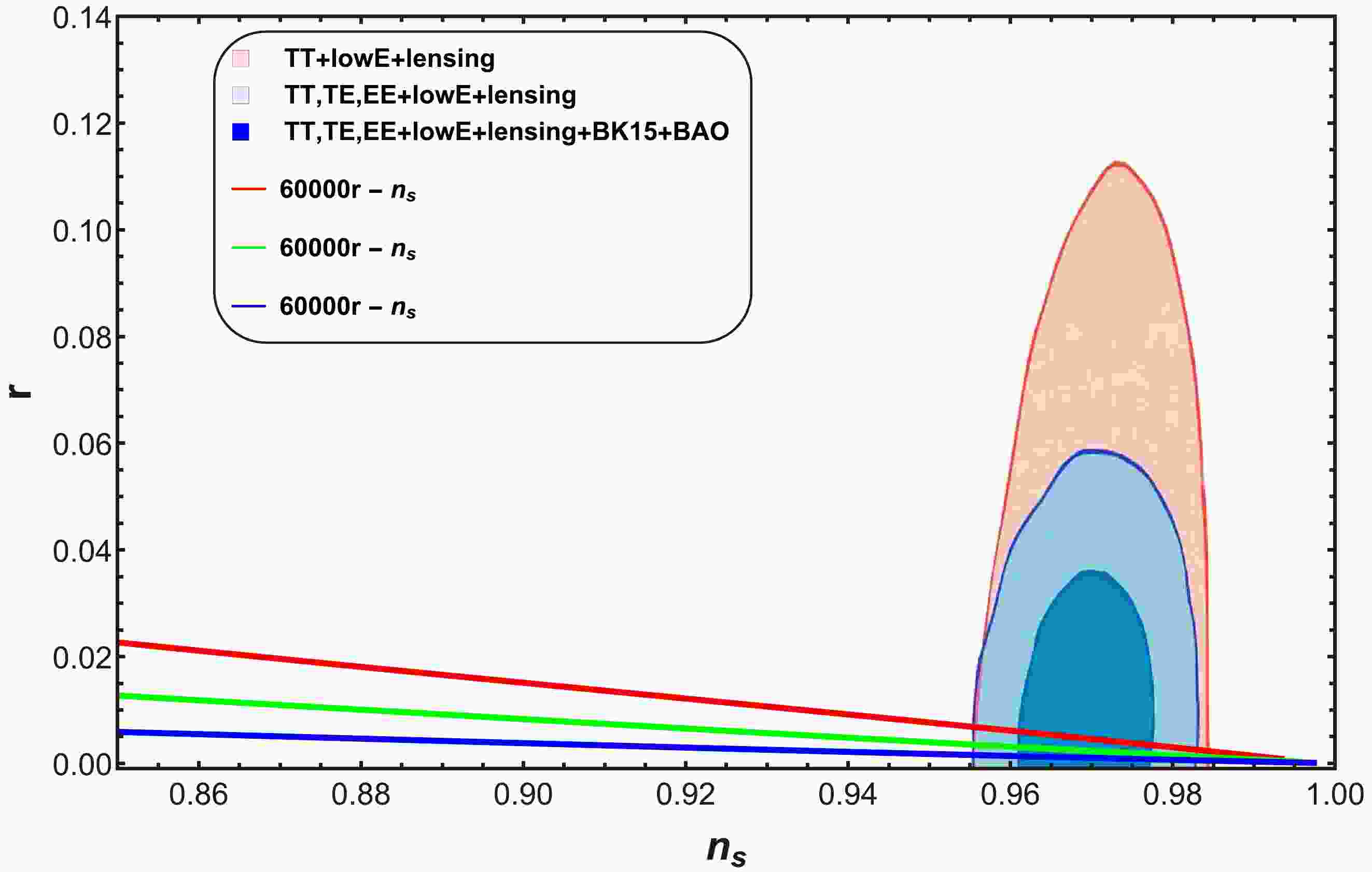
$ n_{s} $ : For the case of a strong dissipative regime, we plot the trajectories of the tensor-to-scalar ratio r versus the scalar spectral index$ n_{s} $ by utilizing Eqs. (33) and (35) for three cases:$ a=0 $ (Fig. 1),$ a=1 $ (Fig. 2), and$ a=-1 $ (Fig. 3). The plot in Fig. 1 corresponds to three different values of the parameter p and h, where$ h=H_{inf} $ [49]. The values of the other parameters are$ C_{\gamma}=70 $ ,$ M_{p}=1 $ ,$ C_1=10^{-35} $ , and$ C_{\phi}=4.39\times10^{-3} $ . The behavior of r decreases for the selected range of$ n_{s} $ . This plot shows that for$ n_{s}=0.9649\pm0.0042 $ , we obtain$ r<0.066 $ , which is reported by the Planck collaboration [47, 48]. In Fig. 2, we present a graph of the tensor-to-scalar ratio r versus the scalar spectral index$ n_{s} $ for the case$ a=1 $ .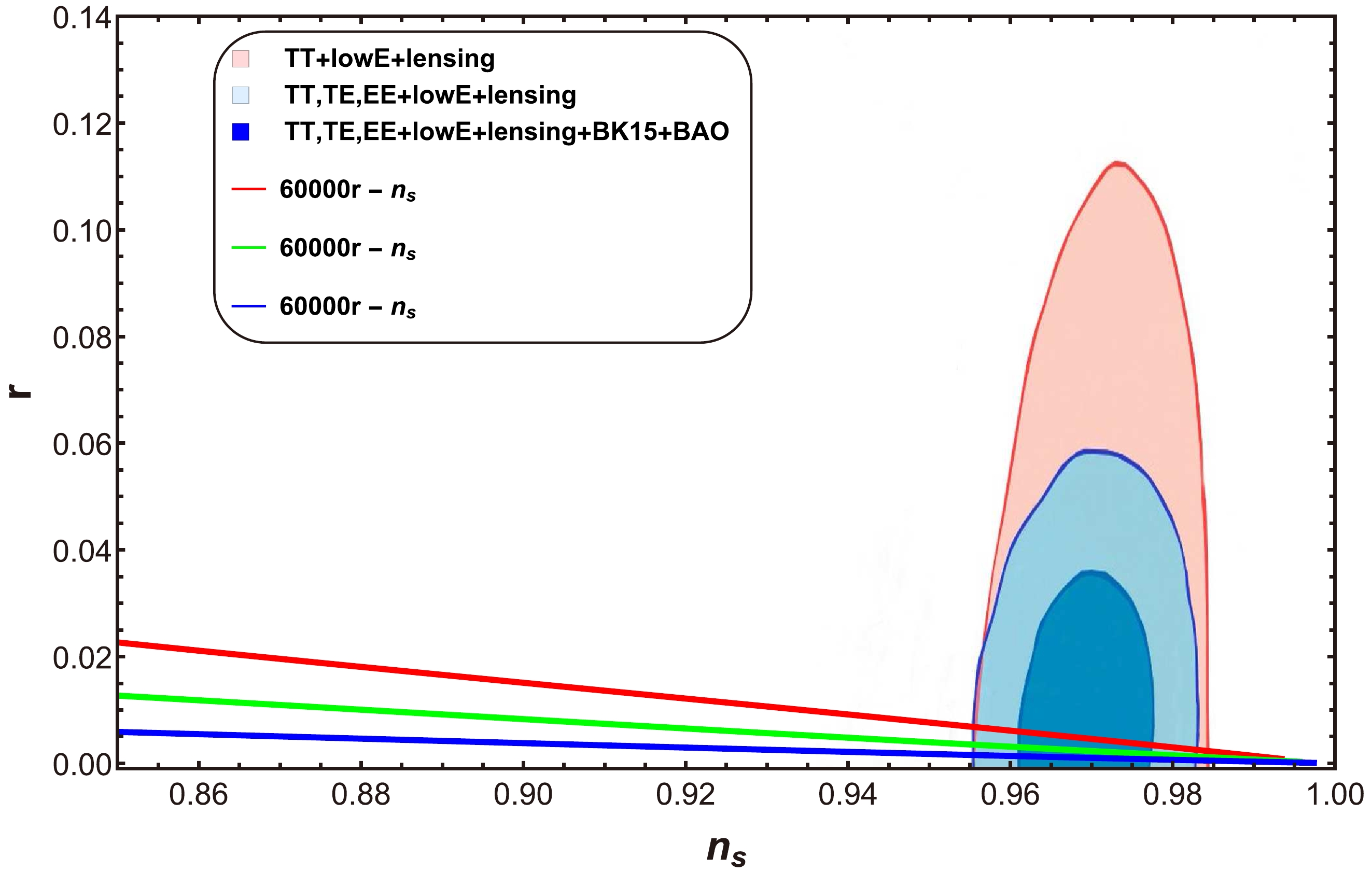
Figure 1. (color online) Plot of tensor-to-scalar ratio r versus scalar spectral index
$ n_{s} $ for$ a=0 $ .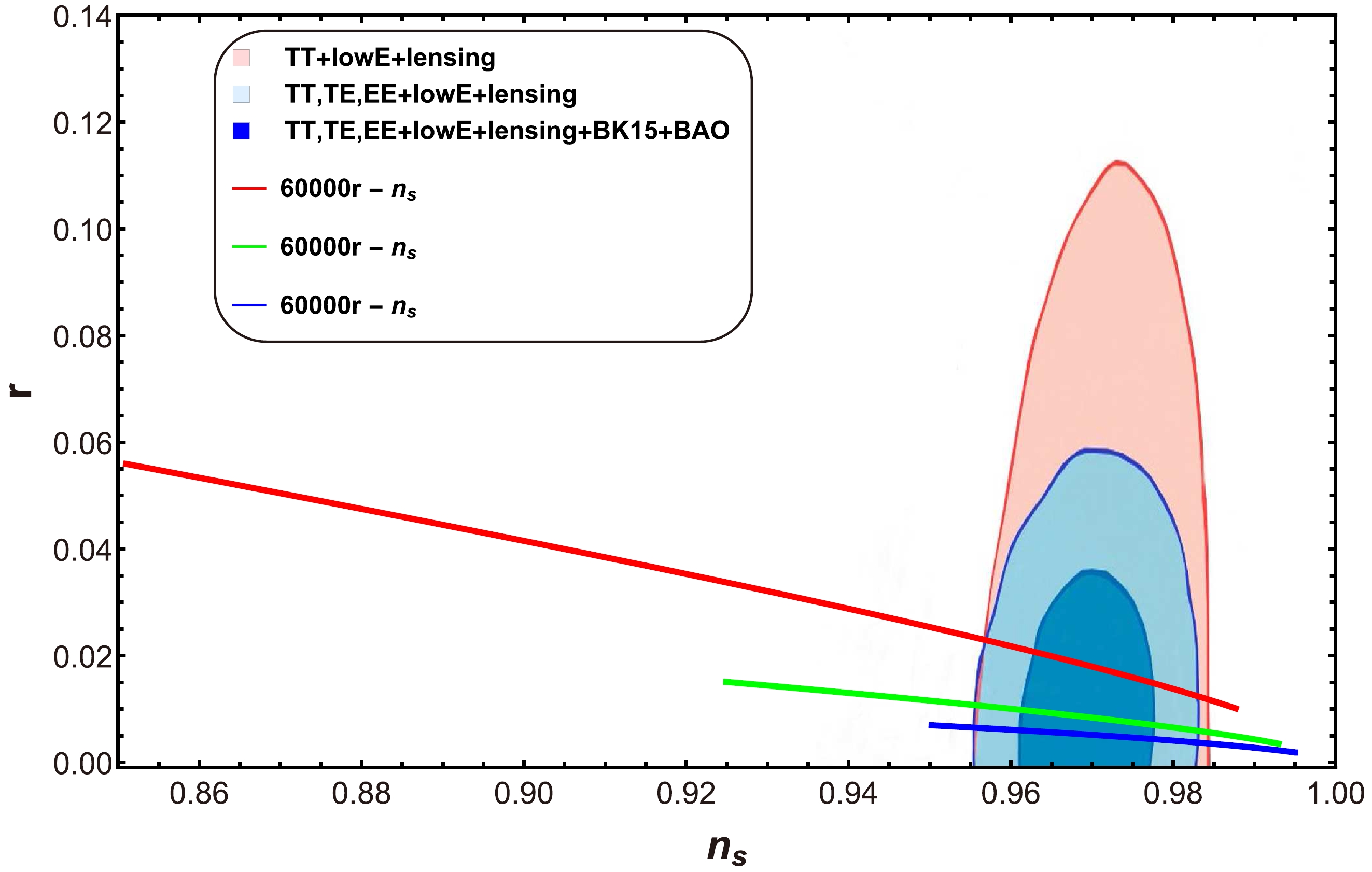
Figure 2. (color online) Graph of tensor-to-scalar ratio r versus scalar spectral index
$ n_{s} $ for$ a=1 $ .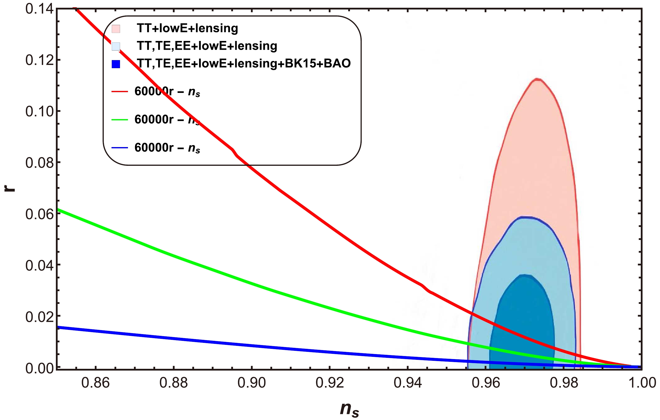
Figure 3. (color online) Plot of tensor-to-scalar ratio r as a function of the scalar spectral index
$ n_{s} $ for$ a=-1 $ .In this plot,
$h=2\times10^{-9}, \; 3\times 10^{-9},4\times10^{-9}$ and$p=3, 5,\; 7$ , and the values of the other parameters remain the same as those in Fig. 1. In this case, the range of values for$ n_s $ and r is also the one given by the Planck collaboration [47, 48]:$ 0.9607<n_s<0.9691 $ and$ 0<r<0.066 $ , respectively. Finally, concerning the underlying potential, Fig. 3 shows the plot of r versus$ n_{s} $ for the case$ a=-1 $ . In this plot,$p=0.52,\; 0.55,\; 0.58,$ and$h=12\times10^{-4},\; 8\times10^{-4}, 4\times10^{-4}$ , and the values of the other parameters remain the same as those in Fig. 1. In this plot, the range of r and$ n_{s} $ are also compatible with Planck data [47, 48]. These three plots confirm the compatibility of our model with the Planck observations. Consequently, the models show consistency with the GCG model for all choices of model parameters.● Behavior of R versus
$ n_{s} $ : Figures 4 and 5 show plots of$R={\Gamma}/{(3H)}$ as a function of the scalar spectral index$ n_{s} $ according to Eqs. (25), (33) and two different cases:$ a=0 $ (Fig. 4) and$ a=1 $ (Fig. 5). In Fig. 4, the general parametrization of the dissipative coefficient$\Gamma(\phi,T) = C_{\phi}{T^{a}}/{\phi^{a-1}}$ takes the form$ \Gamma=C_{\phi}\phi $ . Thus, Eq. (8) becomes$R={C_{\phi}\phi}/{(3H)}$ . In this plot, three different values of the parameters p and h are considered: p = 35.20, 70.20, 105.20,$h=15\times10^{-5},\; 17\times10^{-5}, \; 19\times10^{-5}$ . Other parameters are$ C_{\gamma}=70 $ ,$ C_{\phi}=4\times10^{-4} $ , and$ M_{p}=1 $ .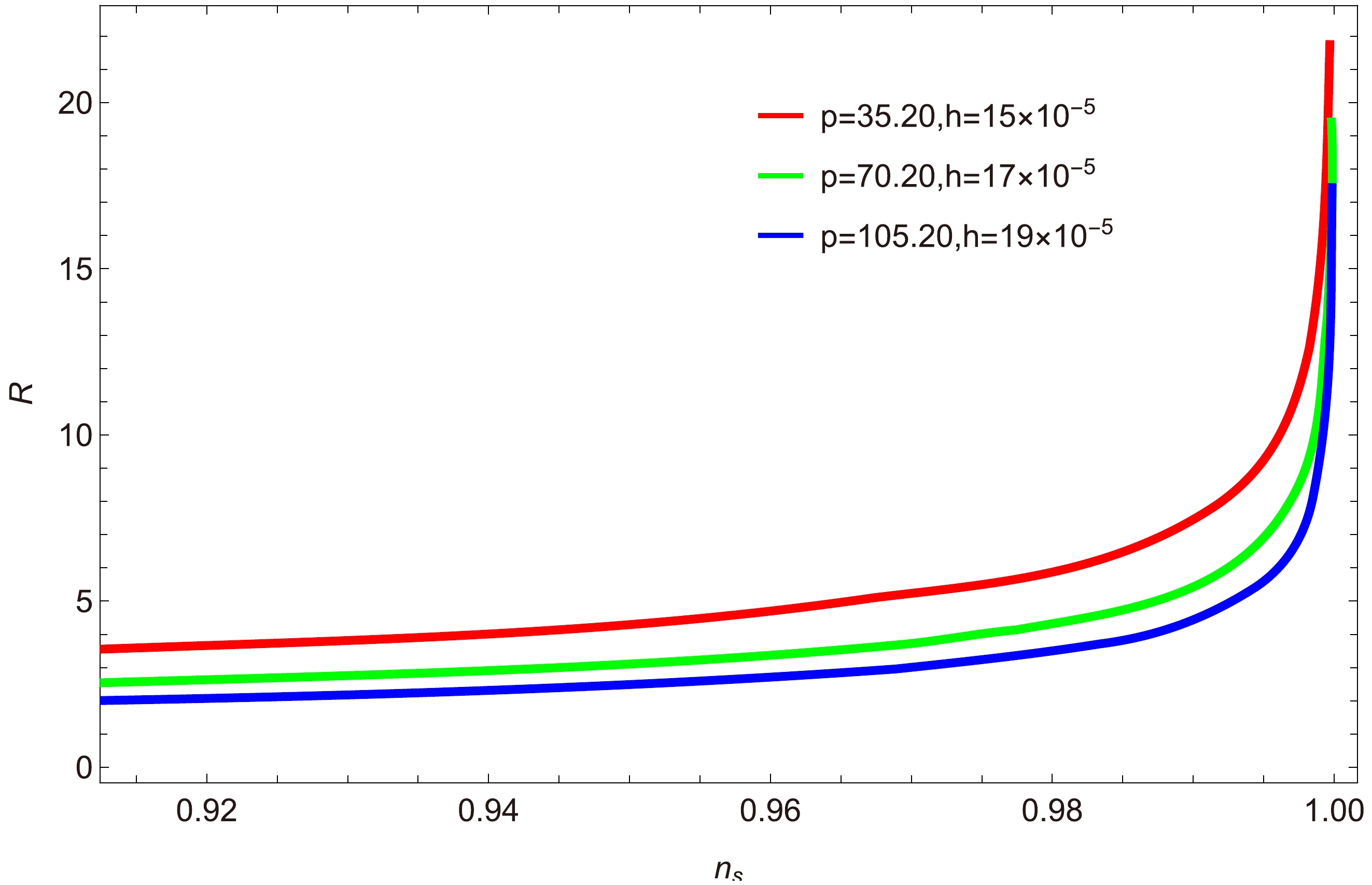
Figure 4. (color online) Plot of
$ R=\dfrac{\Gamma}{3H} $ versus scalar spectral index$ n_{s} $ for$ a=0 $ .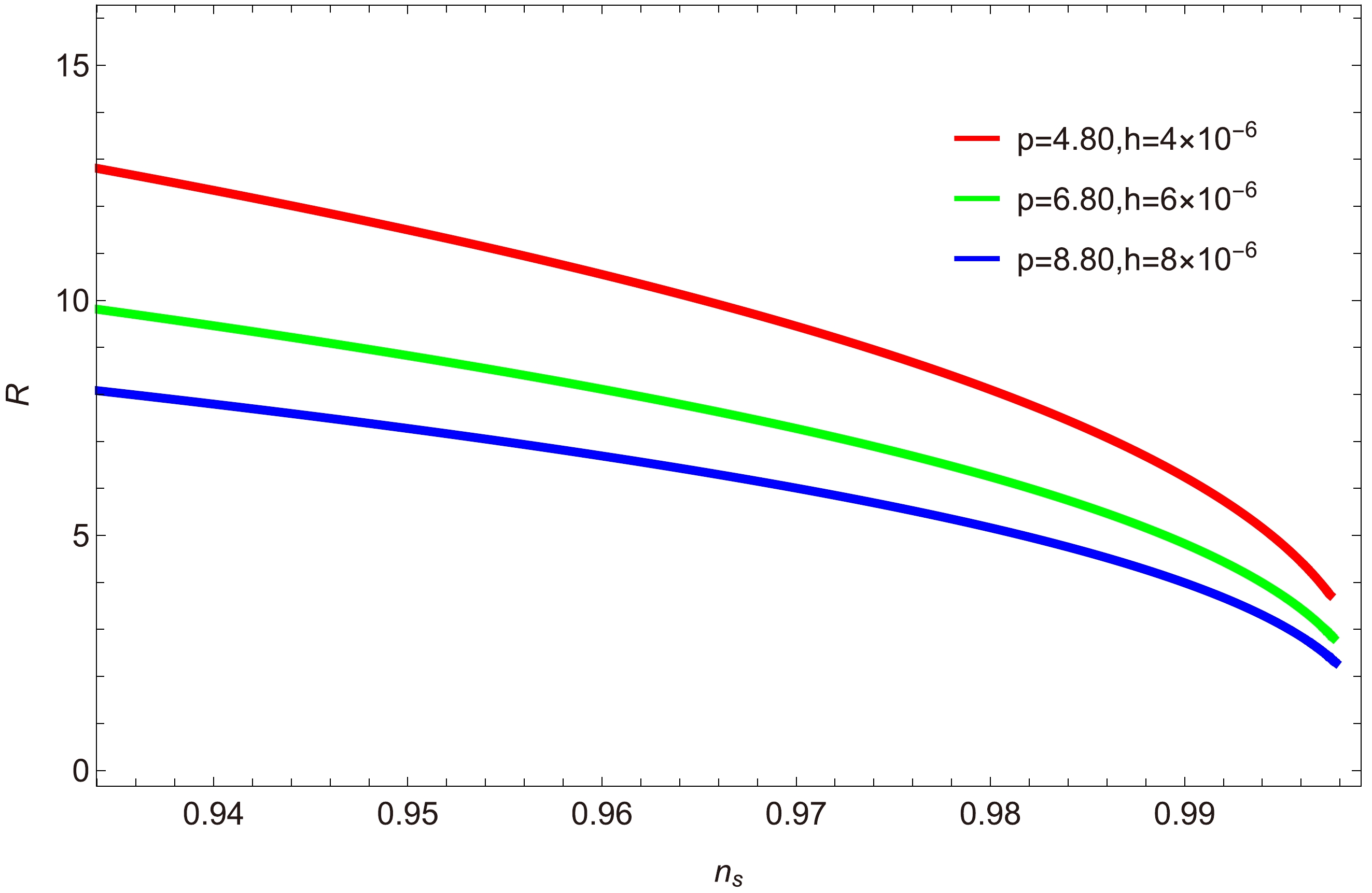
Figure 5. (color online) Plot of
$ R=\dfrac{\Gamma}{3H} $ versus scalar spectral index$ n_{s} $ for$ a=1 $ .Figure 4 clearly shows that for
$ p<105.2 $ and$ h<19\times10^{-5} $ , the model exists in the strong dissipative regime of warm inflation. In Fig. 5, assuming that the model evolves according to the strong dissipative regime$ (R\gg1) $ , we consider three different values of parameters,$ p=4.80,\; 6.80,\; 8.80 $ and$ h=4\times10^{-6},\; 6\times10^{-6},\; 8\times10^{-6} $ , and fixed values for the other parameters:$ C_{\gamma}=70 $ ,$ C_{\phi}=0.439 $ , and$ M_{p}=1 $ . The trajectories of the plot lie in the range$ 0.94\leq n_{s}\leq0.99 $ for$ 0\leq R \leq15 $ . Hence, by considering the essential condition for warm inflation, i.e.,${T}/{H} > 1$ , we obtain the condition for which the model evolves in the strong regime.● Behavior of
$\dfrac{{\rm d}n_{s}}{{\rm d}\ln k}$ and$ n_{s} $ : Planck 2018 collaboration investigated the scale dependence of$ n_s $ . Their results reveal that running in the scalar spectral index leads to a very small negative value close to zero. Figures 6 and 7 show plots depicting the running of the scalar spectral index$\dfrac{{\rm d}n_{s}}{{\rm d}\ln k}$ as a function of$ n_{s} $ for$ a=0 $ and$ a=1 $ , respectively. In Fig. 6, we consider three different values of parameters$ (p,h)=(0.20,\; 4\times 10^{-5}),\; (0.60,\; 6\times10^{-5}) $ , and$ (1.20,\; 8\times10^{-5}) $ . The value of the other parameters are$ C_{\gamma}=70 $ ,$ M_{p}=1 $ , and$ C_{\phi}=15\times10^{-2} $ . For the observational range of$ n_{s}=0.9649\pm0.0042 $ , we obtain the range of the running of the spectral index found by Planck [47, 48], which is$\dfrac{{\rm d}n_{s}}{{\rm d}\ln k}=-0.0126^{+0.0098}_{-0.0087}$ . This prediction suggests that our underlying model is consistent.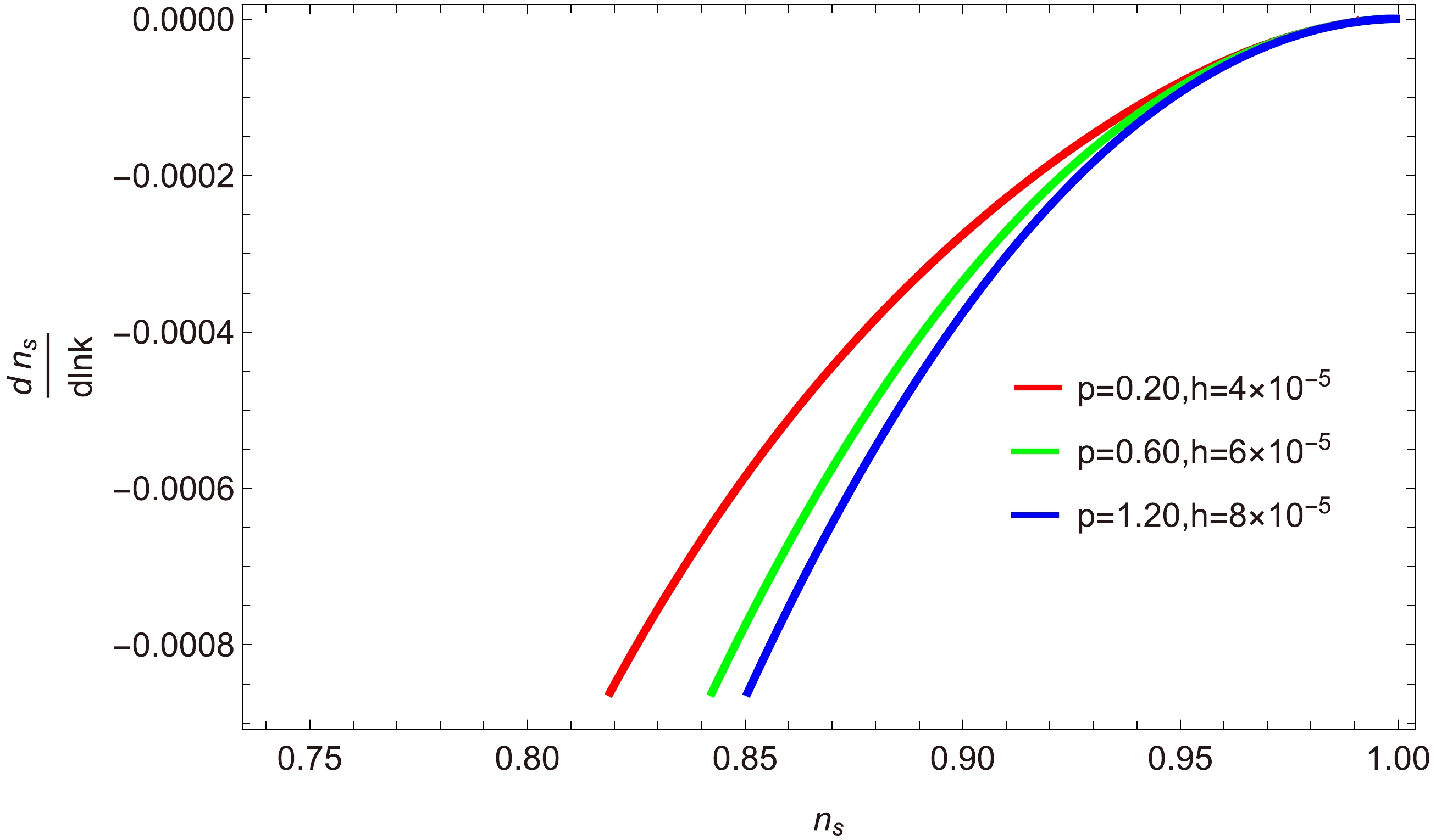
Figure 6. (color online) Plot of running of the scalar spectral index
$\dfrac{{\rm d}n_{s}}{\ln k}$ versus scalar spectral index$ n_{s} $ for$ a=0 $ .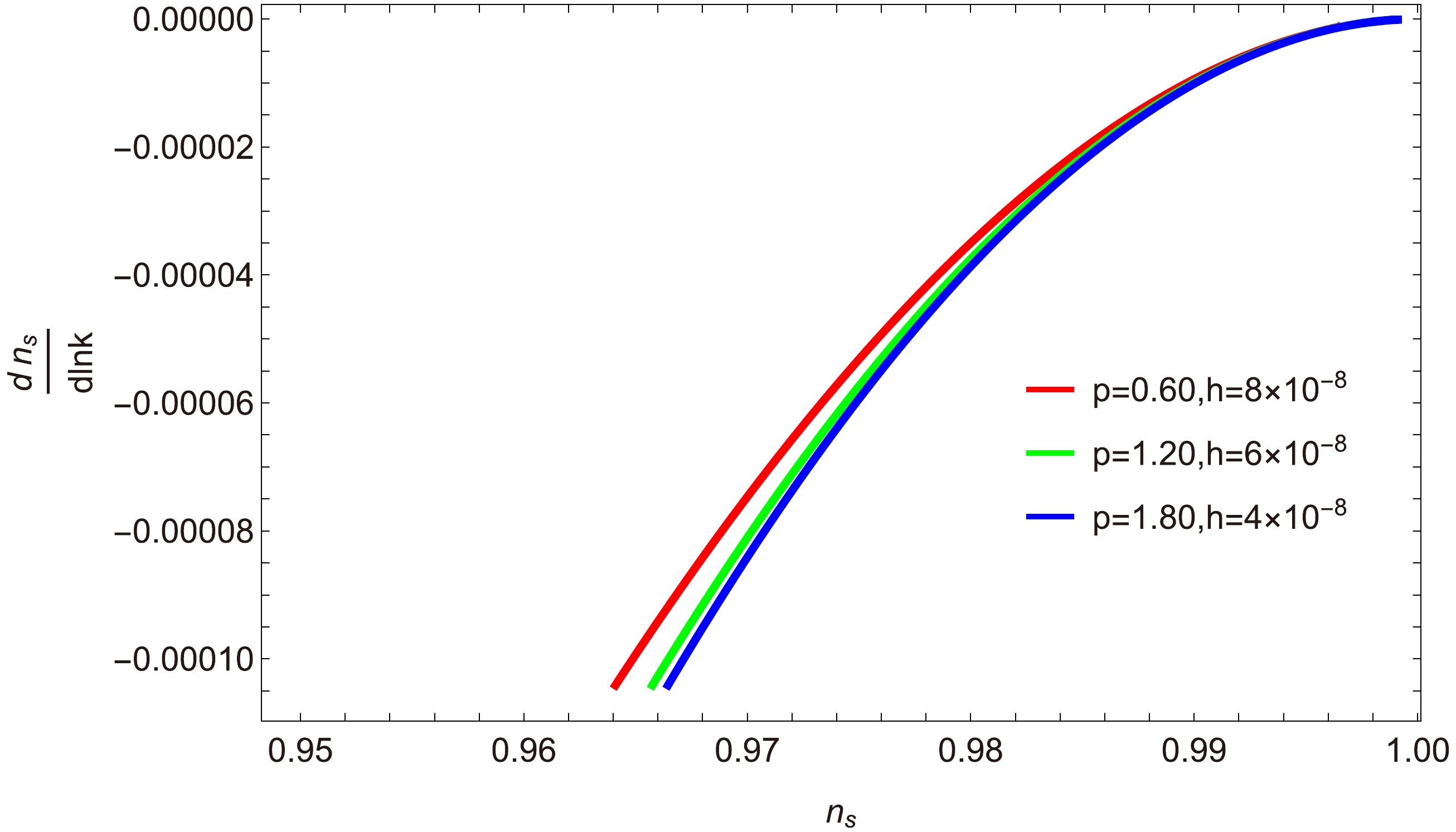
Figure 7. (color online) Graphical behavior of the running of scalar spectral index
$\dfrac{{\rm d}n_{s}}{\ln k}$ versus scalar spectral index$ n_{s} $ for$ a=1 $ .Similarly, in Fig. 7, the pairs of values
$(p,\; h)= (0.60,\; 8\times10^{-8}),\; (1.20,\; 6\times10^{-8})$ and$ (1.80,\; 4\times10^{-8}) $ are represented in red, green, and blue colors, respectively, and the value of the dimensionless parameter is$ C_{\phi}=40.39\times10^{-2} $ . The remaining two parameters are fixed:$ C_{\gamma}=70 $ and$ M_{p}=1 $ . Note in this graph that the running of the spectral index predicted by the model is consistent with the bounds found by Planck [47, 48].● Behavior of
$ {\dfrac{T'V}{TV'}} $ versus$ n_{s} $ : Figures 8 and 9 show plots illustrating the relationship between the scalar spectral index$ n_{s} $ and the ratio$ \dfrac{T'V}{V'T} $ for three different values of p and h. In Fig. 8 (where$ a=0 $ ), we consider$ p=0.100,\; 0.110 $ , and$ 0.120 $ , and$ h=15\times10^{-12},\; 30\times10^{-12} $ and$ 45\times10^{-12} $ . The values$ C_{1}=1\times10^{-35} $ and$ C_{\gamma}=70 $ are fixed in each case, while$ C_{\phi}=2\times10^{3} $ . It is evident that all the trajectories decrease within the selected range of$ n_s $ , and the ratio satisfies the condition$ \dfrac{T'V}{V'T}<1 $ , thereby meeting the swampland conjectures.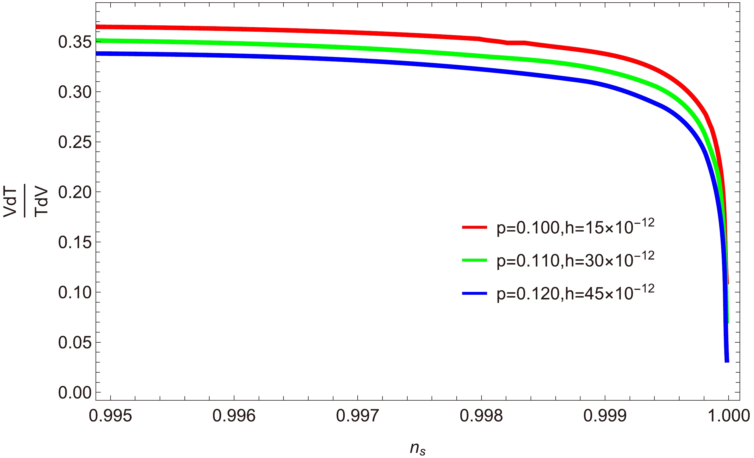
Figure 8. (color online) Plot of ratio
$ {\dfrac{T'V}{TV'}} $ versus$ n_{s} $ for$ a=0 $ .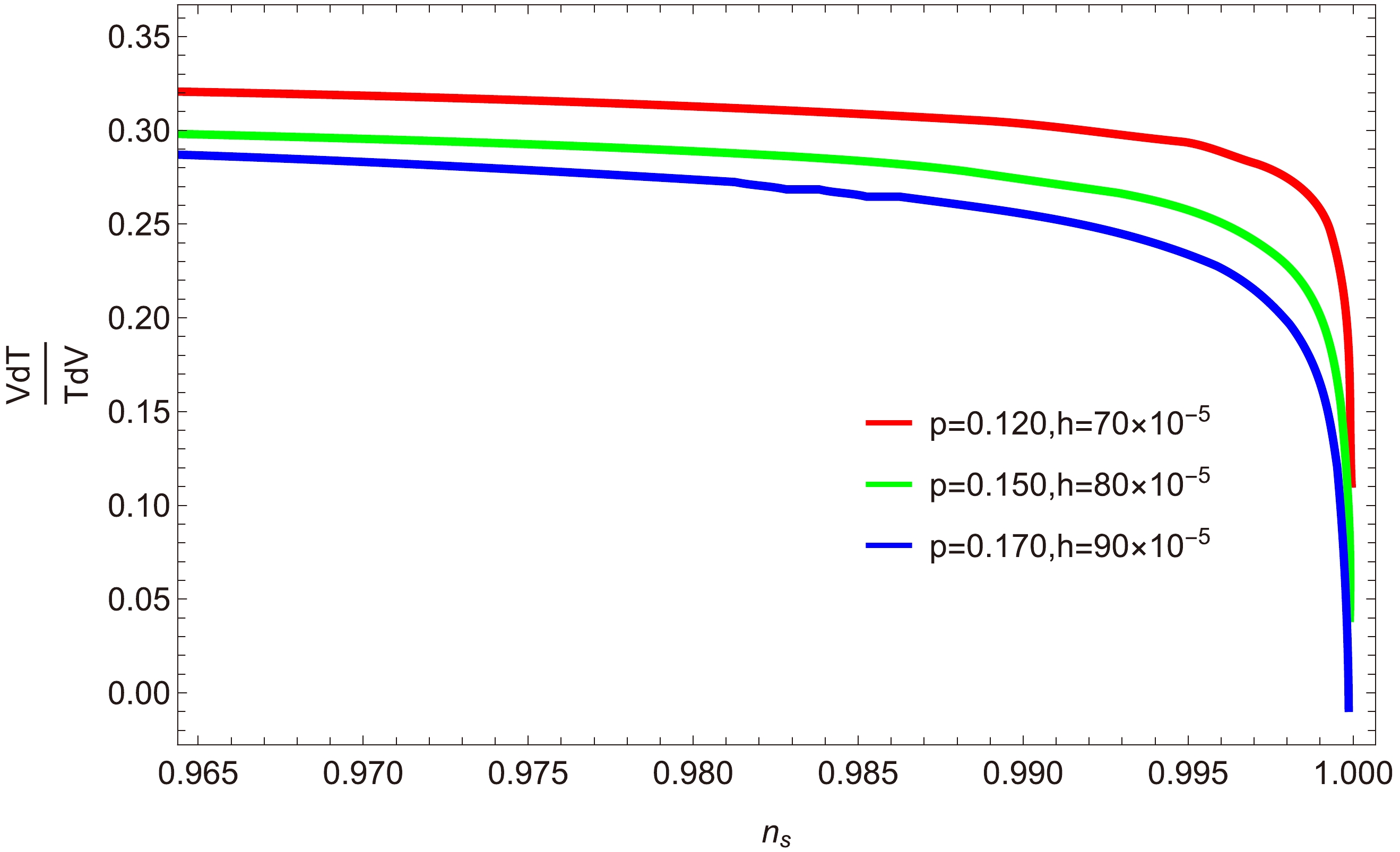
Figure 9. (color online) Plot of ratio
$ {\dfrac{T'V}{TV'}} $ versus$ n_{s} $ for$ a=1 $ .Furthermore, in Fig. 9 (where
$ a=1 $ ), we plot$ \dfrac{T'V}{V'T} $ versus$ n_{s} $ for$ p=0.120,\; 0.150 $ , and$ 0.170 $ , with$h= 70\times10^{-5},\; 80\times10^{-5}$ , and$ 90\times10^{-5} $ . Note from this plot that$ \dfrac{T'V}{V'T}<1 $ , demonstrating the validity of the swampland conjectures. Detain discussion and comparison can be seen in Table 1 and Table 2.For $V=\dfrac{3}{8 \pi}H_{\rm inf}{\rm e}^{\frac{2\phi}{p(\phi+1)} }$ 

a $ n_s $ 

r $\dfrac{{\rm d}n_{s} }{{\rm d}\ln k}$ 

$ \dfrac{T'V}{TV'} $ 

0 $ [0.93,1] $ 

$ [0,1\times10^{-7}] $ 

[−0.0002,0] $<1 $ 

1 $ [0.9,1] $ 

$ [0,8\times10^{-7}] $ 

[−0.00010,0] $<1 $ 

−1 $ [0.93,1] $ 

$ [0,2\times10^{-7}] $ 

$ - $ 

$ - $ 

$ V=M^{4}\bigg(\dfrac{\phi}{M_{p}}\bigg)^{2}\bigg(1+\dfrac{\beta\phi^{2}}{M^{2}_{p}}\bigg) $ 

a $ n_s $ 

r $\dfrac{{\rm d}n_{s} }{{\rm d}\ln k}$ 

$ \dfrac{T'V}{TV'} $ 

0 $ [0.938,0.994] $ 

$ [0,1.4\times10^{-6}] $ 

$ [-0.0001,0.0004] $ 

$<1 $ 

1 $ [0.96,1] $ 

$ [0,2\times10^{-8}] $ 

$ [-0.00005,0.0002] $ 

$<1 $ 

−1 $ [0.954,1] $ 

$ [0,3\times10^{-6}] $ 

$ [-0.000004,0.00002] $ 

$<1 $ 

$V=\dfrac{3}{4}M^{2}(1-{\rm e}^{ {\sqrt{\frac{2}{3} } }\phi})^{2}$ 

a $ n_s $ 

r $\dfrac{{\rm d}n_{s} }{{\rm d}\ln k}$ 

$ \dfrac{T'V}{TV'} $ 

0 $ [0.916,1.005] $ 

$ [0,0.0013] $ 

$ [-0.00017,0] $ 

$<1 $ 

1 $ [0.906,0.966] $ 

$ [0,0.0004] $ 

$ [-0.00013,-0.00005] $ 

$<1 $ 

−1 $ [0.936,1.103] $ 

$ [0,0.00023] $ 

$ [-0.0002,0] $ 

$<1 $ 

Parameter $ Planck $ TT,TE,EE+lowEB+lensing

$ Planck $ TT,TE,EE+lowE+lensing+BK15

$ Planck $ TT,TE,EE+lowE+lensing+BK15+BAO

$ n_s $ 

$ 0.9659 \pm 0.0041 $ 

$ 0.9651 \pm 0.0041 $ 

$ 0.9668 \pm 0.0037 $ 

r $<0.11 $ 

$<0.061 $ 

$<0.063 $ 

α $ -0.0085 \pm 0.0073 $ 

$ -0.0069 \pm 0.0069 $ 

$ -0.0066 \pm 0.0070 $ 

Table 2. Observational data (Akrami et al. 2018 [51]).
-
This model is a generalization of the large field inflation model
$ V(\phi)\propto \phi^p $ . The motivation for investigating mixed large field inflation arises from the aim to enrich our understanding of the early universe's dynamics by exploring a broader spectrum of inflaton field behaviors. Unlike traditional inflationary models, which predominantly focus on either small or large field values, mixed large field inflation considers scenarios where the inflaton traverses both regimes during its evolution. This approach is motivated by the desire to capture a more diverse and realistic range of field dynamics that may have occurred across different regions of the universe. This potential reads as [50]$ V = M^{4}\bigg(\frac{\phi}{M_{p}}\bigg)^{2}\bigg(1+\beta\frac{\phi^{2}}{M^{2}_{p}}\bigg). $

where
$ \beta=\dfrac{M}{M_{p}} $ , M is the mass scale, and$ M_{p} $ is Plank's reduced mass; we set$ M_{p}=1 $ . This model includes a single parameter denoted as β. Given that the exact magnitude of this parameter is not initially known, it is assumed that a Jeffreys prior distribution is applied to β. By repeating the above procedure for this potential, we obtain the equations of dissipative ratio R, scalar spectral index$ n_{s} $ , tensor to-scalar-ratio r, amplitude of power spectrum$ {{\cal{P}}_{{\cal{R}}}}^{\frac{1}{2}} $ , and ratio$ {\dfrac{T' V}{TV'}} $ in Appendix B. -
● Behavior of r versus
$ n_{s} $ : In the case of mixed large field inflation, we present plots of the tensor-to-scalar ratio r and scalar spectral index$ n_{s} $ for three cases,$ a=0 $ ,$ a=1 $ , and$ a=-1 $ , in Figs. 10, 11, and 12, respectively. Figure 10 shows the trajectories for$ \beta=21,\; 24,\; 28 $ , where β is defined as$\beta={M}/{M_{p}}$ (with M representing the mass scale) and$ C_{\phi}=4.39\times10^{-2} $ . From this plot, we determine that the compatible range of Planck data, with$ n_{s}=0.9649\pm0.0042 $ , results in$ r<0.066 $ . We observe a similar behavior of trajectories in the other two cases (Figs. 11 and 12). Therefore, the three plots confirm the compatibility of our model with the latest observational dataset [47, 48].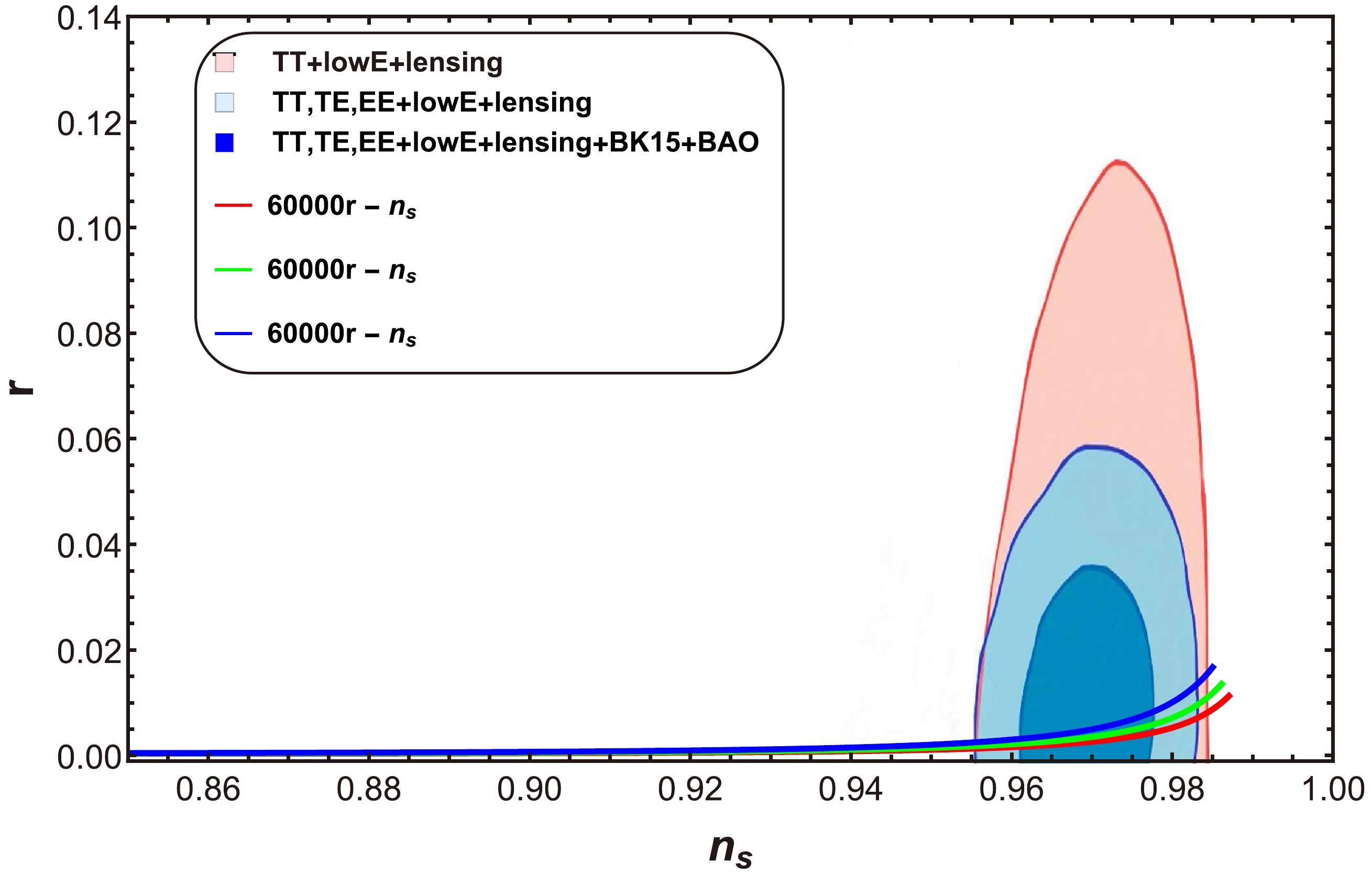
Figure 10. (color online) Plot of r versus
$ n_{s} $ for$ a=0 $ .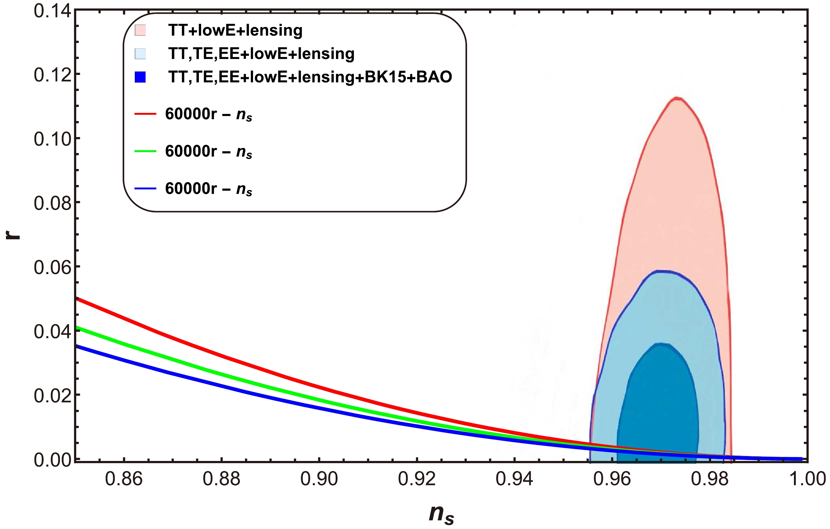
Figure 11. (color online) Plot of r versus
$ n_{s} $ for$ a=1 $ .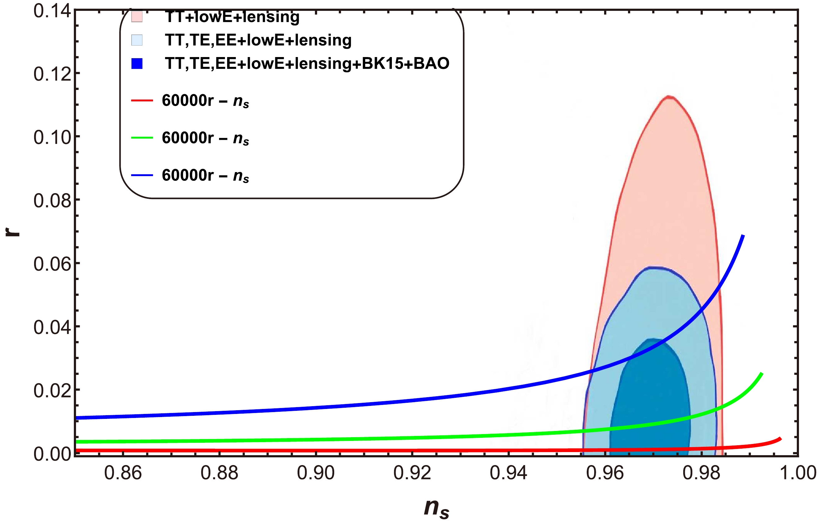
Figure 12. (color online) Plot of r versus
$ n_{s} $ for$ a=-1 $ .● Behavior of
$\dfrac{{\rm d}n_{s}}{{\rm d}\ln k}$ versus$ n_{s} $ : Figures 13, 14, and 15 show the relationship between the scalar spectral index$ n_{s} $ and the running of the spectral index$\dfrac{{\rm d}n_{s}}{{\rm d}\ln k}$ for the strong dissipative regime$ (R\gg1) $ . We explore three different cases of a, specifically$ a=0,\; 1,\; -1 $ , for three different values of β. Figure 13 shows thatwithin the range$ 0.92<n_{s}<0.98 $ , we obtain$\dfrac{{\rm d}n_{s}}{{\rm d}\ln k}$ , implying that the underlying model is consistent. For$ a=1 $ , Fig. 14 shows that the range of$\dfrac{{\rm d}n_{s}}{{\rm d}\ln k}$ lies in the interval$ [0.0000, 0.0006] $ for the selected value of$ n_s $ , and the trajectories of$\dfrac{{\rm d}n_{s}}{{\rm d}\ln k}$ decrease when$ n_s>0.92 $ . This small range indicates that the given model is consistent. Similarly, in Fig. 15, the trajectories of$\dfrac{{\rm d}n_{s}}{{\rm d}\ln k}$ approach zero within the observational range of$ n_s $ , demonstrating a well-matched result with Planck data [47, 48].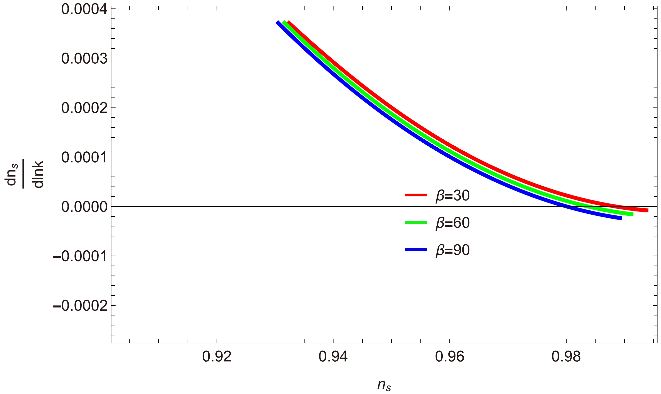
Figure 13. (color online) Plot of
$\dfrac{{\rm d}n_{s}}{{\rm d}\ln k}$ versus$ n_{s} $ for$ a=0 $ .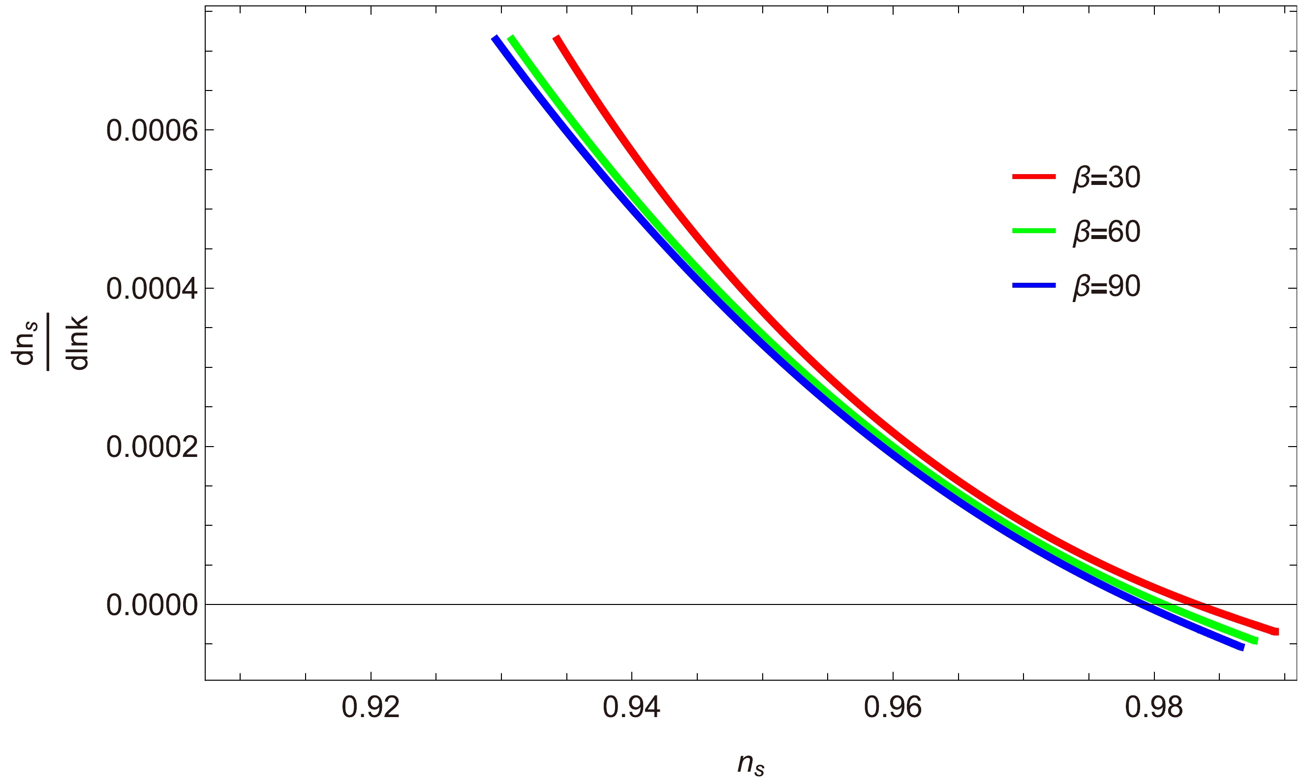
Figure 14. (color online) Plot of
$\dfrac{{\rm d}n_{s}}{{\rm d}\ln k}$ versus$ n_{s} $ for$ a=1 $ .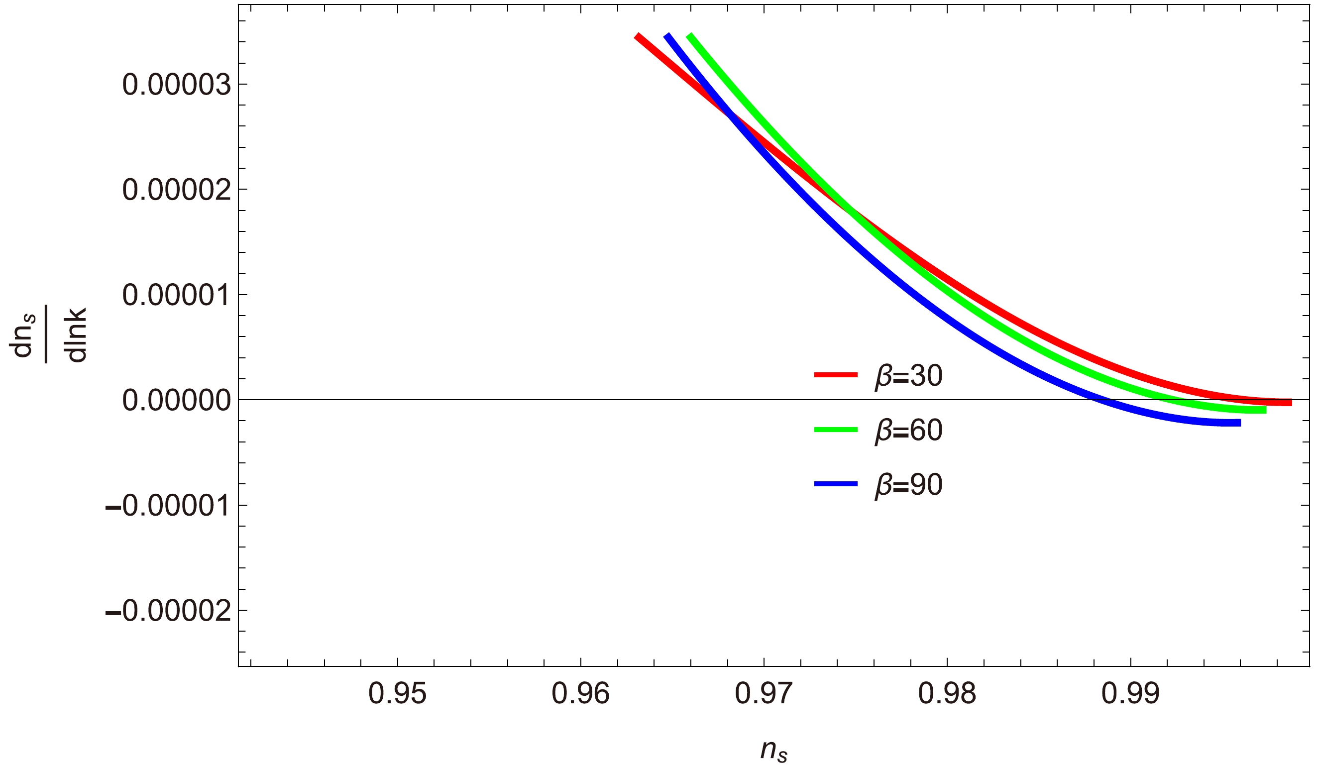
Figure 15. (color online) Plot of
$\dfrac{{\rm d}n_{s}}{{\rm d}\ln k}$ versus$ n_{s} $ for$ a=-1 $ .● Behavior of
$ \dfrac{T'V}{TV'} $ versus$ n_{s} $ : We next analyze the de-Sitter swampland conjecture constraints through the ratio$ \dfrac{T'V}{V'T} $ represented as a function of the scalar spectral index$ n_{s} $ in Figs. 16, 17, and 18 for different values of β. In Fig. 16, we consider 68% confidence limits of the scalar spectral index,$ 0.94\lesssim n_s\lesssim0.99 $ . Within this range,$ \dfrac{T'V}{V'T}<1 $ , satisfying the required swampland conjectures. In the other two figures, we obtain results similar to those shown in Fig. 16.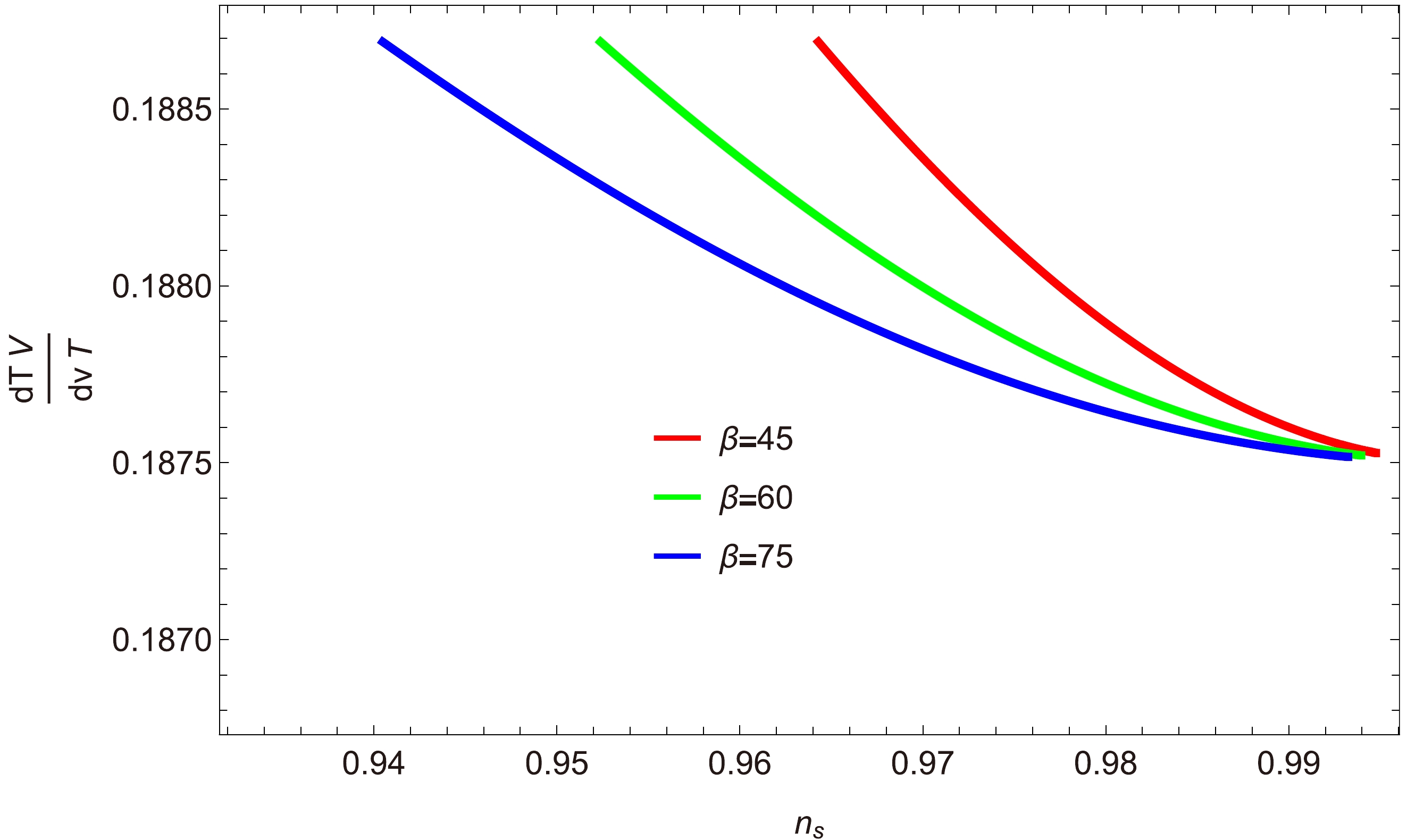
Figure 16. (color online) Plot of
$ \dfrac{T'V}{TV'} $ versus$ n_{s} $ for$ a=0 $ .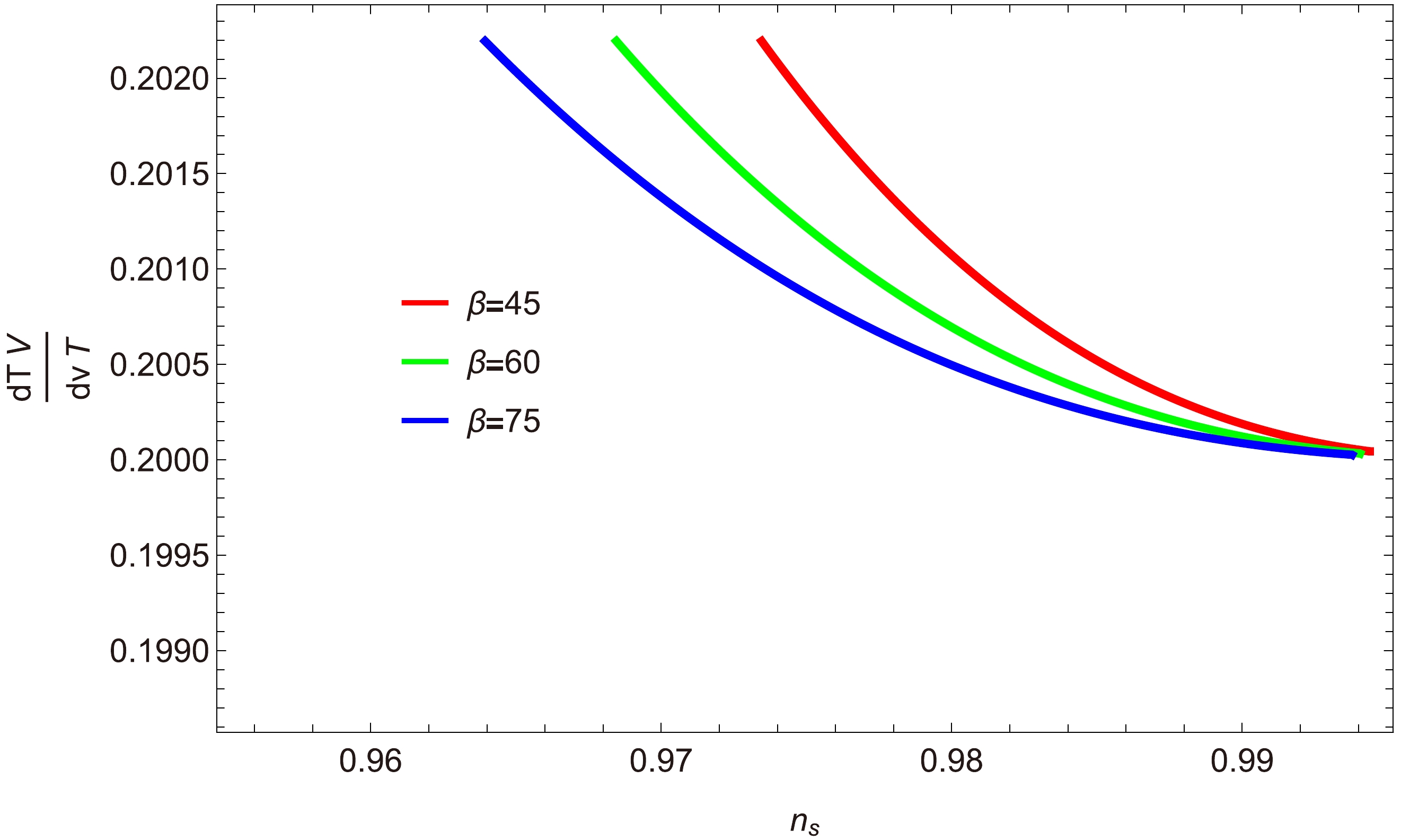
Figure 17. (color online) Plot of
$ \dfrac{T'V}{TV'} $ versus$ n_{s} $ for$ a=1 $ .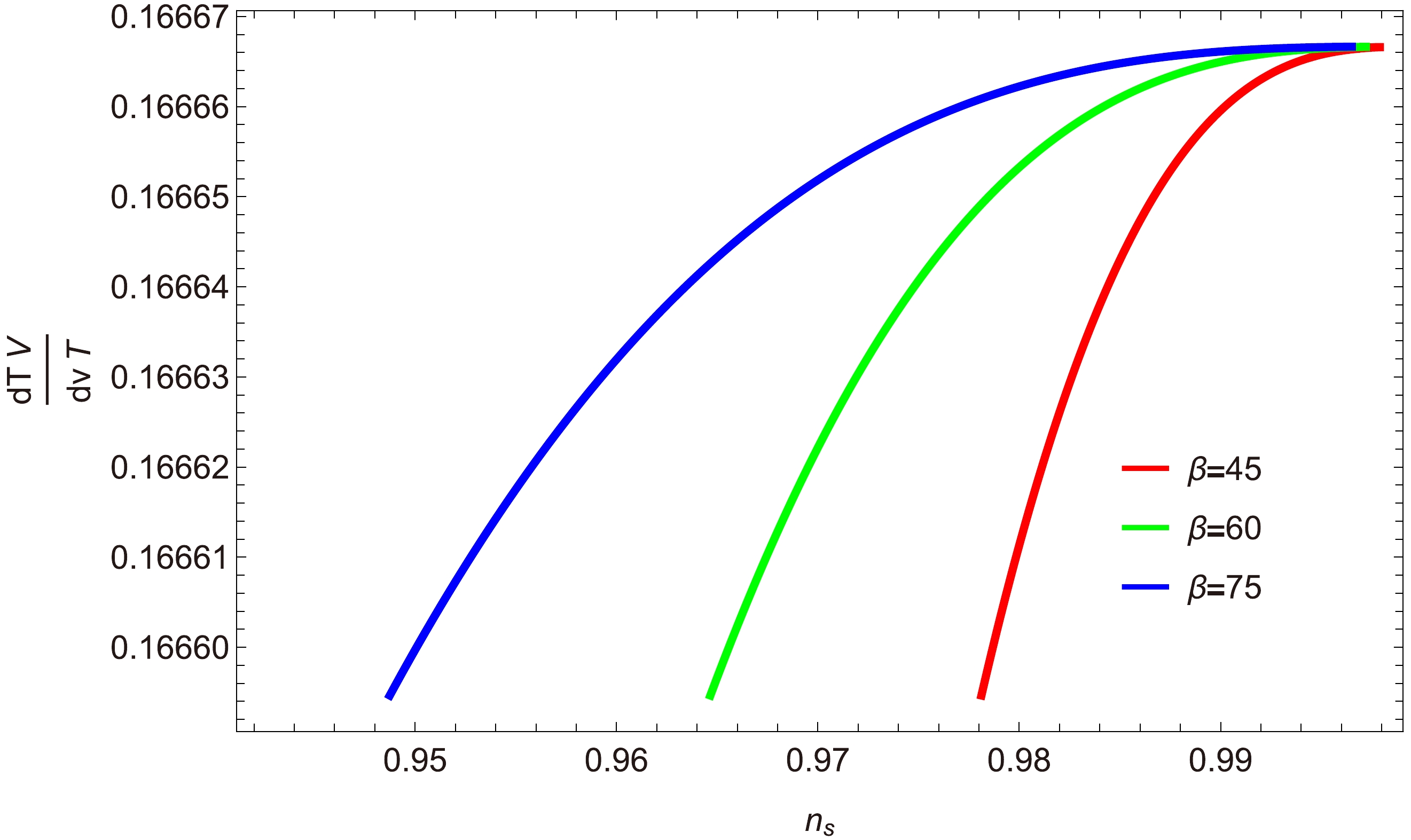
Figure 18. (color online) Plot of
$ \dfrac{T'V}{TV'} $ versus$ n_{s} $ for$ a=-1 $ . -
The exponential potentials naturally exhibit a power-law behavior, offering a simple and tractable form that facilitates analytical treatment. This simplicity allows for a more straightforward analysis of the inflationary dynamics and its consequences. We consider a single-field exponential potential expressed as [49]
$ V = \frac{3}{4}M^{2}(1-{\rm{e}}^{{\sqrt{\frac{2}{3}}}\phi})^{2}, $

where M is the mass scale. The equations of dissipative ratio R, curvature perturbation
$ {{\cal{P}}_{{\cal{R}}}} $ , scalar spectral index$ n_{s} $ , running of the scalar spectral index$\dfrac{{\rm d}n_{s}}{{\rm d}\ln k}$ , and ratio$ {\dfrac{\acute{T} V}{T \acute{V}}} $ for strong regime$ (R\gg1) $ are derived in Appendix C. -
● Behavior of r Vs
$ n_{s} $ : Figures 19, 20, and 21 show plots of the trajectories of the tensor-to-scalar ratio r as a function of the scalar spectral index$ n_s $ for small variations in the values of M. It is evident that all the trajectories are generally consistent with recent observations from Planck 2018 [47, 48]. Specifically, they remain in the region$ r<0.066 $ for the selected values of$ n_s $ 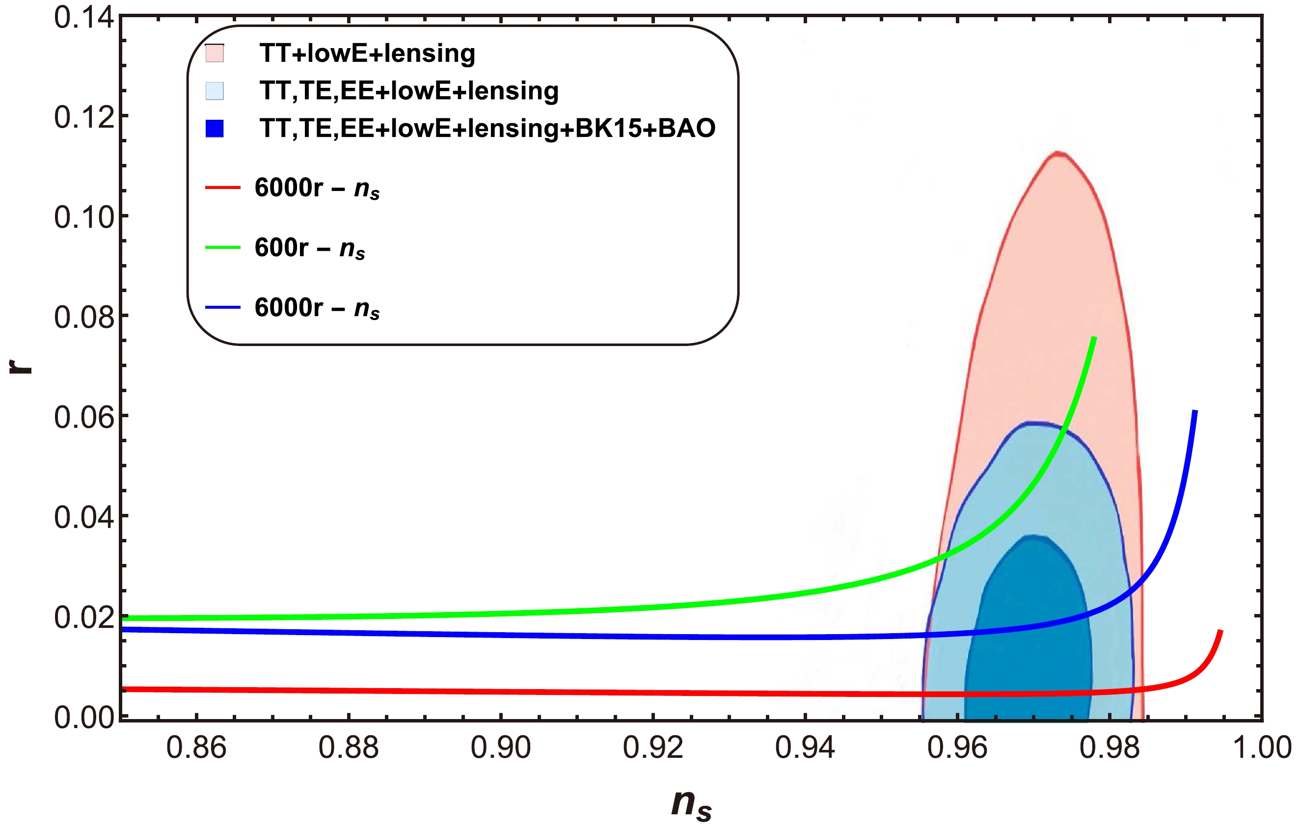
Figure 19. (color online) Plot of r versus
$ n_{s} $ for$ a=0 $ .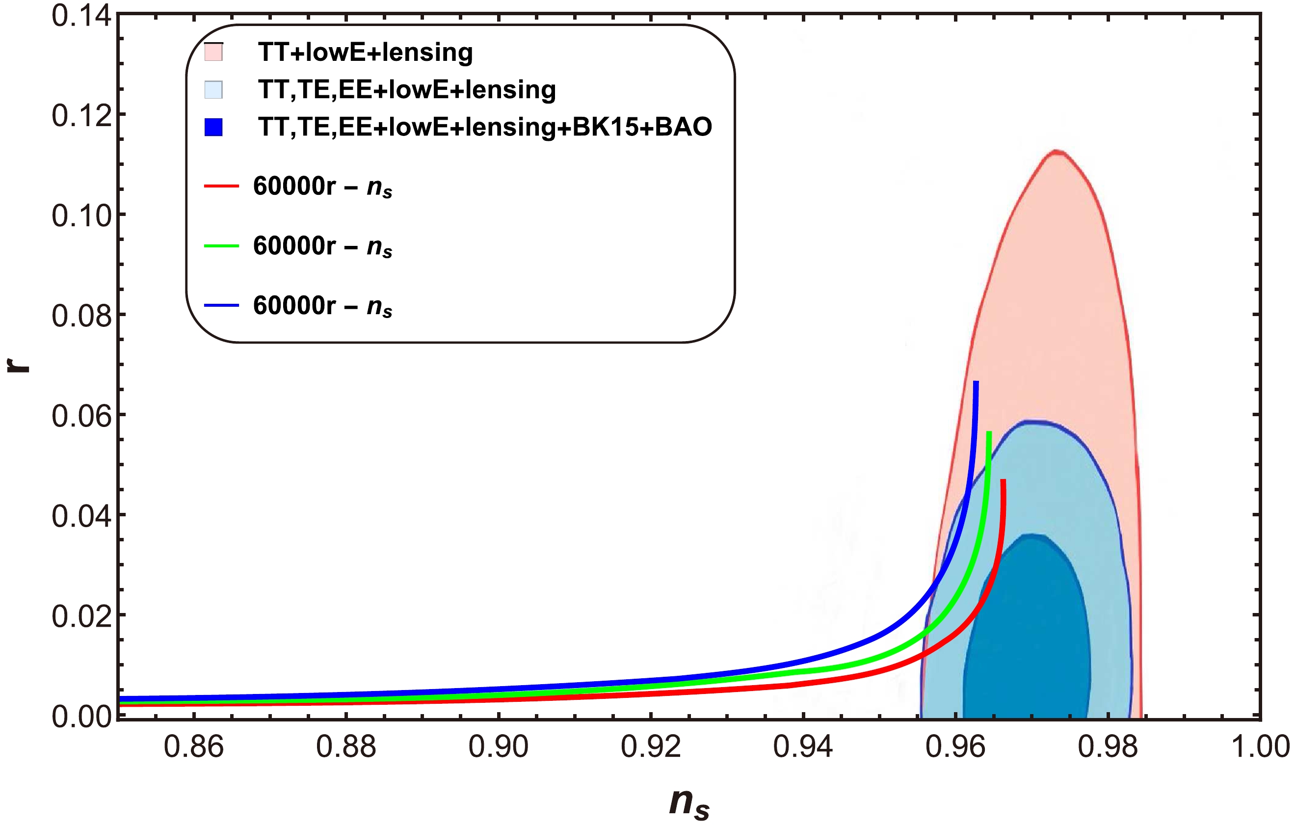
Figure 20. (color online) Plot of r versus
$ n_{s} $ for$ a=1 $ .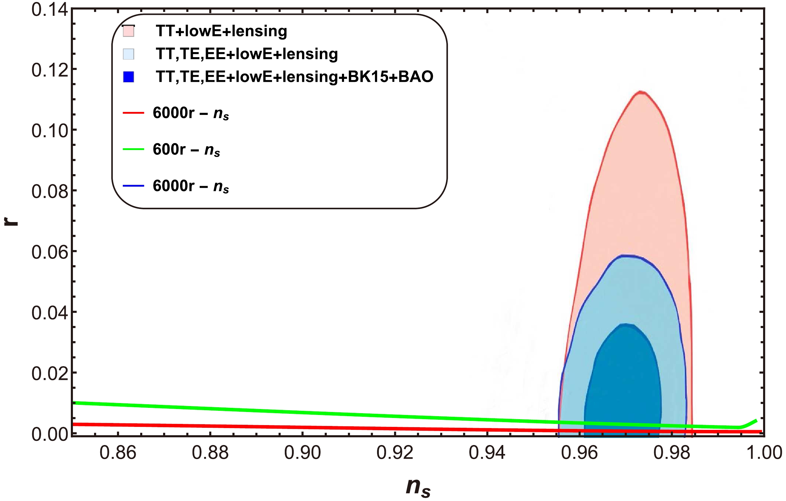
Figure 21. (color online) Plot of r versus
$ n_{s} $ for$ a=-1 $ .● Behavior of
$\dfrac{{\rm d}n_{s}}{{\rm d}\ln k}$ versus$ n_{s} $ : Figures 22, 23, and 24 show the relationship between the running of the scalar spectral index$\dfrac{{\rm d}n_{s}}{{\rm d}\ln k}$ and the scalar spectral index$ n_{s} $ for three inflationary decay rates:$ a=0,\; 1,\; -1 $ . Figure 22 shows that for the case$ a=0 $ , the trajectories of$ n_{s} $ and$\dfrac{{\rm d}n_{s}}{{\rm d}\ln k}$ fall within the intervals$ [0.94, 1.00] $ and$ [-0.00015, 0.00000] $ . This small negative range of$\dfrac{{\rm d}n_{s}}{{\rm d}\ln k}$ confirms the compatibility of our model withrecent observational data. Similarly, in Figs. 23 and 24, the range of the running of the scalar spectral index is$-0.00015\lesssim\dfrac{{\rm d}n_{s}}{{\rm d}\ln k}\lesssim0.00007$ and$-0.0005\lesssim \dfrac{{\rm d}n_{s}}{{\rm d}\ln k}\lesssim0$ , respectively. These small negative ranges align with the Planck data set [47, 48].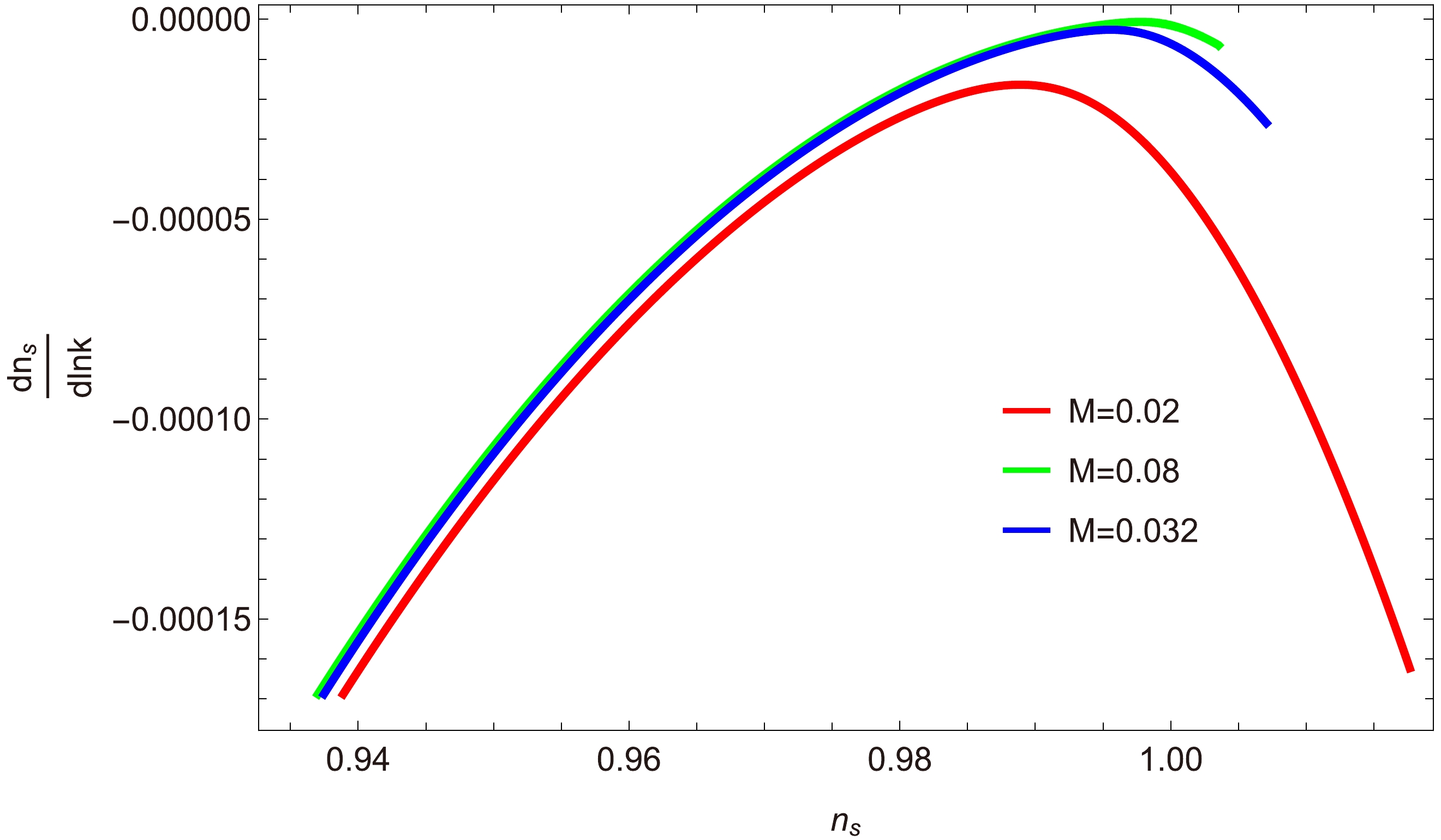
Figure 22. (color online) Plot of
$\dfrac{{\rm d}n_{s}}{{\rm d}\ln k}$ versus$ n_{s} $ for$ a=0 $ .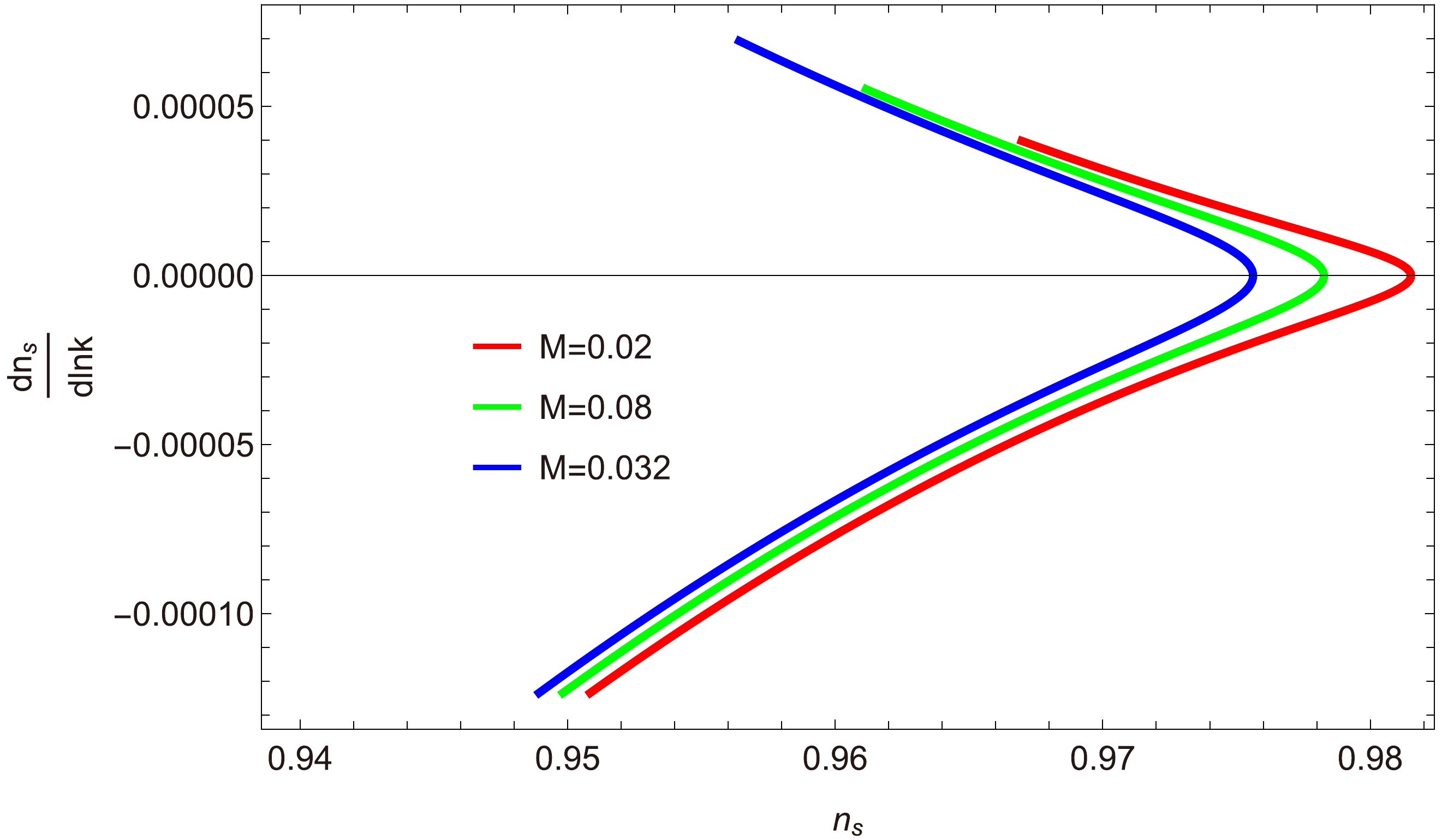
Figure 23. (color online) Plot of
$\dfrac{{\rm d}n_{s}}{{\rm d}\ln k}$ versus$ n_{s} $ for$ a=1 $ .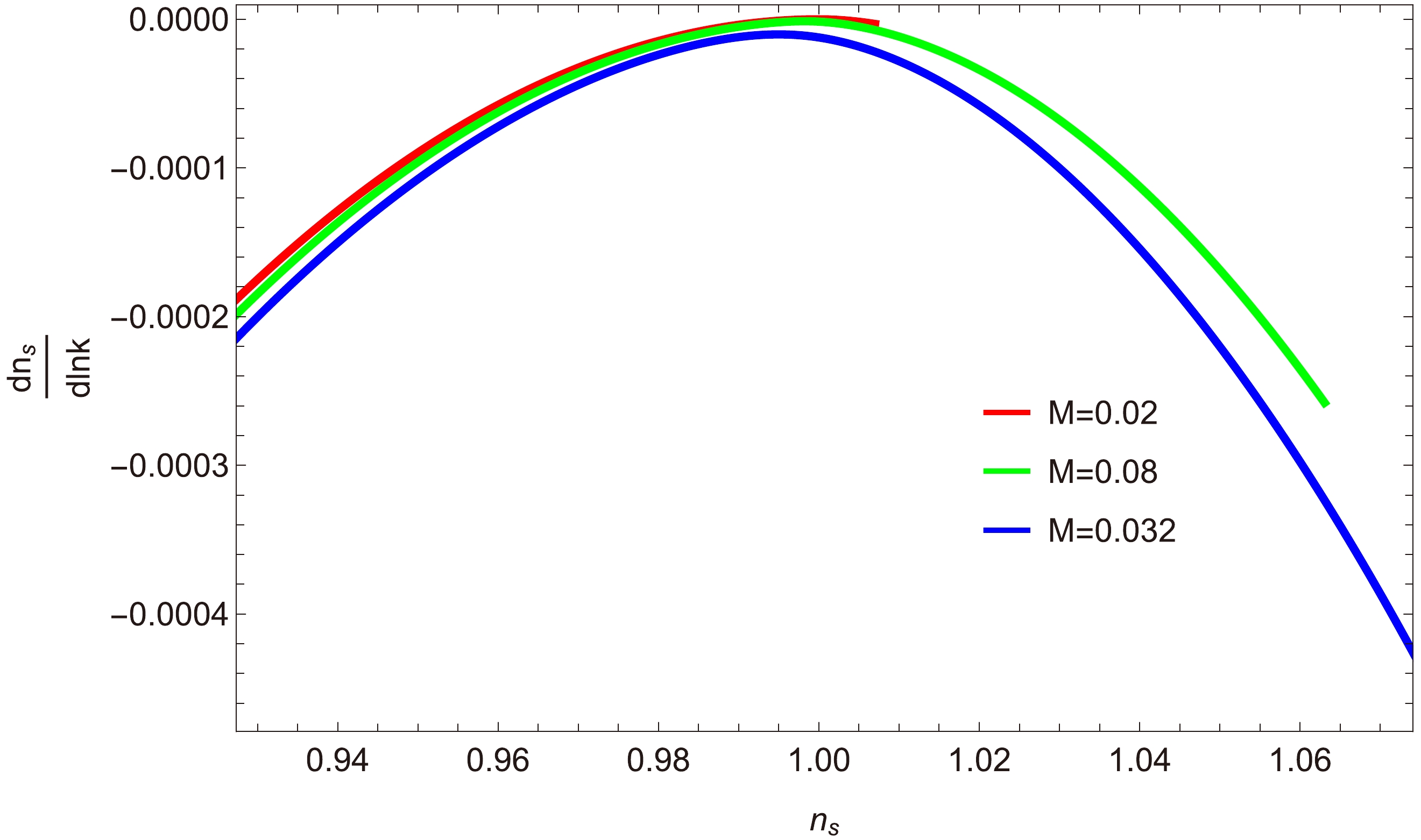
Figure 24. (color online) Plot of
$\dfrac{{\rm d}n_{s}}{{\rm d}\ln k}$ versus$ n_{s} $ for$ a=-1 $ .● Behavior of
$ \dfrac{T'V}{TV'} $ versus$ n_{s} $ : Figures 25, 26, and 27 depict the relationship between the generalized ratio of the de-Sitter conjecture$ \dfrac{T'V}{TV'} $ and the scalar spectral index$ n_{s} $ , for three inflationary decay rates:$ a=0, 1, -1 $ . These figures clearly show that$ \dfrac{T'V}{TV'}<1 $ , demonstrating the validity of the swampland conjectures.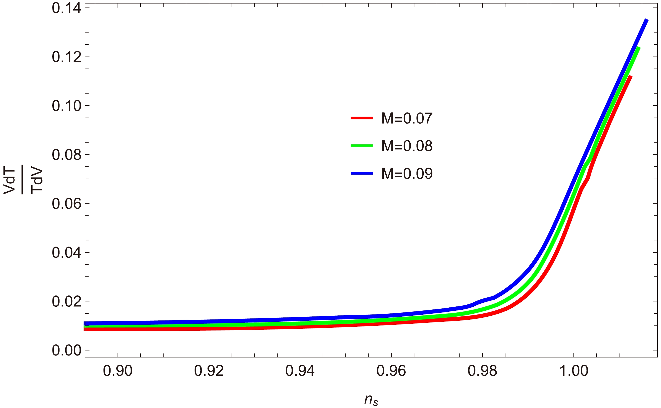
Figure 25. (color online) Plot of
$ \dfrac{T'V}{TV'} $ versus$ n_{s} $ for$ a=0 $ .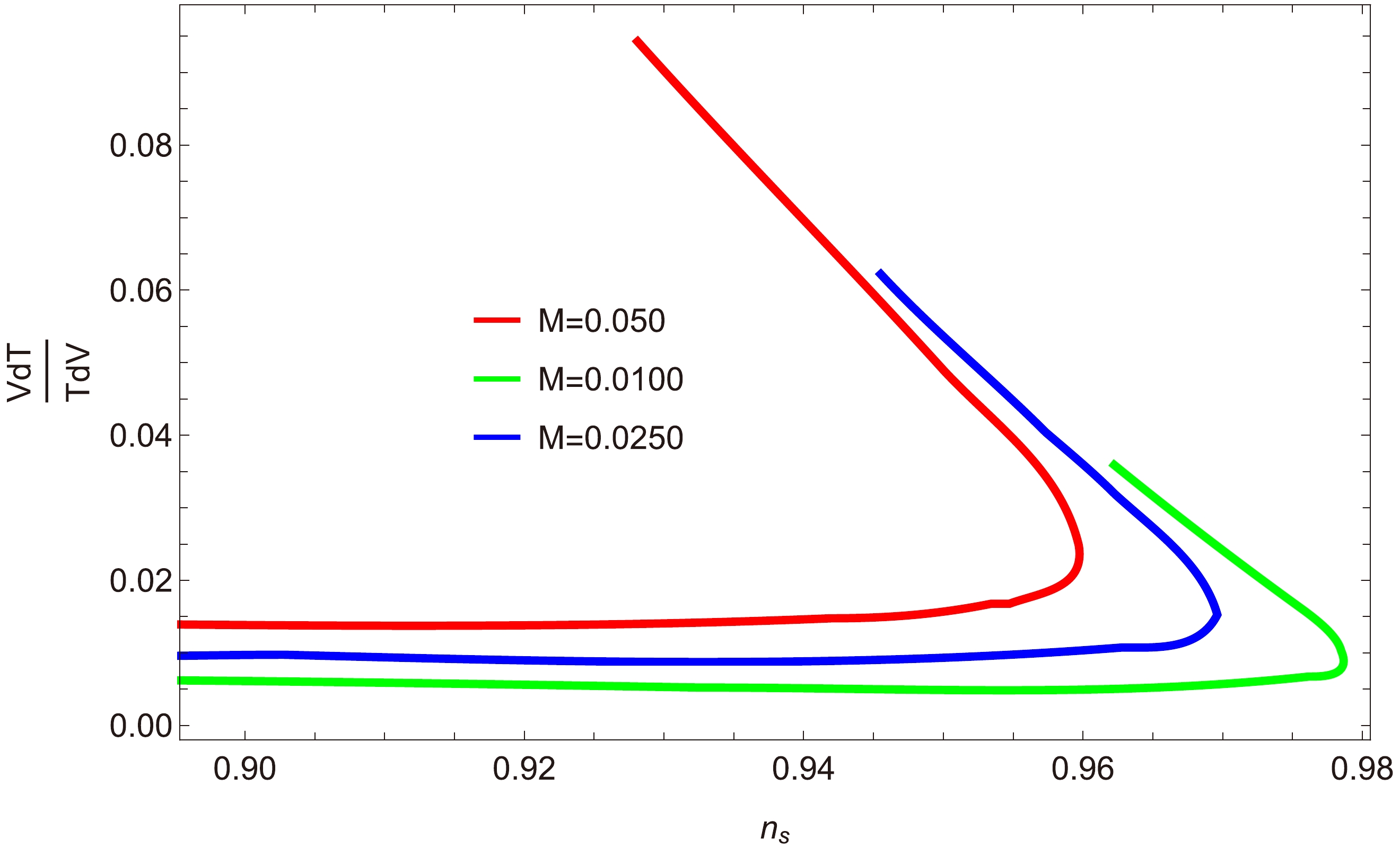
Figure 26. (color online) Plot of
$ \dfrac{T'V}{TV'} $ versus$ n_{s} $ for$ a=1 $ .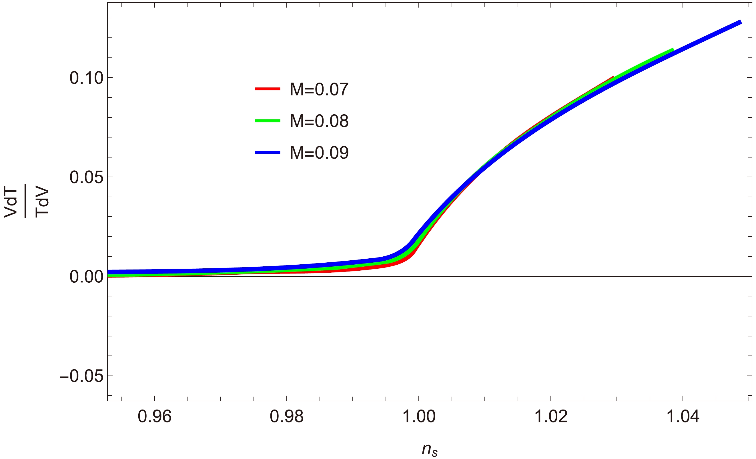
Figure 27. (color online) Plot of
$ \dfrac{T'V}{TV'} $ versus$ n_{s} $ for$ a=-1 $ . -
In this paper, we have focused on the outcomes from considering another family of single-field inflation models, namely power-law plateau inflation, within the context of warm inflation, inspired from CG and GCG models. To elucidate the dissipative effects during inflationary expansion, we have focused on a generalized expression for the inflation decay ratio given by
$ \Gamma(\phi, T)= $ $C_{\phi}\dfrac{T^{a}}{\phi^{a-1}} $ , where$ a=0, 1, -1 $ denote three different inflationary decay rates. These decay rates are associated with the potentials$V=\dfrac{3}{8\pi}H_{\rm inf}{\rm e}^{\frac{2\phi}{p(\phi+1)}}$ ,$ V=M^{4}\bigg(\dfrac{\phi}{M_{p}}\bigg)^{2}\bigg(1+\dfrac{\beta\phi^{2}}{M^{2}_{p}}\bigg) $ , and$ V=\dfrac{3}{4}M^{2}(1-{\rm e}^{{\sqrt{\frac{2}{3}}}\phi})^{2} $ , which represent different inflationary decay ratios studied in the literature. Our focus has been on the strong dissipative regime, where$ R\gg1 $ . Within this dissipative regime, we have applied slow-roll approximations to discuss both the background and perturbative dynamics of these inflation models.We have also calculated the expressions of the scalar power spectrum
$ {{\cal{P}}_{{\cal{R}}}} $ , scalar spectral index$ n_{s} $ , running scalar spectral index$\dfrac{{\rm d}n_{s}}{{\rm d}\ln k}$ , dissipative ratio R, and ratio$ \dfrac{T'V}{TV'} $ . For each potential, we have obtained the observational range of all inflationary parameters:$ r<0.066 $ ,$ n_s=0.9661\pm0.0040 $ , and$\dfrac{{\rm d}n_s}{{\rm d}\ln k}=-0.006\pm0.013$ [47, 48]. We have also checked the validity of the swampland conjectures through the ratio$ \dfrac{T'V}{TV'} $ . In every case, we have found that this ratio lies in the interval$ (0,1) $ , which satisfies the required swampland conjectures. It is interesting to remark that all our results confirm the compatibility of our model with observational data. The following tables (Table 1 and Table 2) constitute a detailed discussion of our findings. -
For the quasi-exponential potential
$V(\phi)=\dfrac{3H_{\rm inf}^2}{8\pi}{\rm{e}}^{\frac{2\phi}{p(\phi+1)}}$ , the set of slow-roll parameters takes the form$ \epsilon = -\frac{1}{2}\bigg(\frac{2}{p(1+\phi)}-\frac{2\phi}{p(1+\phi)^2}\bigg)^2, $

(A1) $ \begin{aligned}[b] \eta =\;& {\rm{e}}^{\frac{4\phi}{p(1+\phi)}}\bigg[\frac{-4}{p(1+\phi)^{3}}+\bigg(\frac{2}{p(1+\phi)} -\frac{2\phi}{p(1+\phi)^{2}}\bigg)^{2}\bigg],\\ \beta =\;& \bigg(3^{\frac{5}{2 (a+4)}} 256^{-\frac{1}{a+4}} \pi ^{-\frac{2}{a+4}} \bigg(\dfrac{{\rm{e}}^{\frac{4 \phi }{p (\phi +1)}} H_{\inf }^4 \phi^{a-1} \bigg(\dfrac{2} {p (\phi +1)}-\frac{2 \phi }{p (\phi +1)^2}\bigg)^2}{C_{\phi } C_{\gamma } \sqrt[4]{\dfrac{9 {\rm{e}}^{\frac{4 \phi }{p (\phi +1)}} H_{\inf }^4}{64 \pi ^2}+{C_{1}}}}\bigg)^{\frac{1}{a+4}}\bigg)^{-a}\\ &\times \bigg(3^{\frac{5}{2(a+4)}}256^{-\frac{1}{a+4}}\pi^{-\frac{2}{a+4}}\bigg(\frac{{\rm{e}}^{\frac{4 \phi }{p (\phi +1)}} H_{\inf }^4 \phi^{a-1} \bigg(\dfrac{2}{p (\phi +1)}- \dfrac{2 \phi }{p (\phi +1)^2}\bigg)^2}{C_{\phi } C_{\gamma } \sqrt[4]{\dfrac{9 {\rm{e}}^{\frac{4 \phi }{p (\phi +1)}} H_{\inf }^4} {64 \pi^2}+{C_{1}}}}\bigg)^{\frac{-(a+3)}{(a+4)}}\\ &\times \bigg(\frac{2}{p (\phi +1)}-\frac{2 \phi }{p (\phi+1)^2}\bigg)^{\frac{1}{a+4}}\bigg(\frac{{\rm{e}}^{\frac{4 \phi }{p (\phi +1)}} H_{\inf }^4 \phi^{a-1} \bigg(\dfrac{2}{p(\phi+1)}-\dfrac{2 \phi }{p (\phi+1) ^2}\bigg)^2}{C_{\phi } C_{\gamma } \sqrt[4]{\dfrac{9 {\rm{e}}^{\frac{4 \phi}{p (\phi +1)}} H_{\inf }^4}{64 \pi ^2}+{C_{1}}}}\times \frac{\phi^{a-1}}{C_{\phi }} \bigg) ^{\frac{1}{a+4}}\bigg)^{a-1}\\&\times\bigg[ \frac{\bigg(\bigg((a-1){\rm{e}}^{\frac{4\phi} {p(\phi +1)}} \bigg(\dfrac{2}{p (\phi +1)}-\dfrac{2 \phi } {p (\phi +1)^2}\bigg)^2 H_{\inf }^4 \phi ^{a-2}}{{C_{\phi } C_{\gamma } \sqrt[4]{\dfrac{9 {\rm{e}}^{\frac{4 \phi }{p(\phi+1)}}H_{\inf}^4}{64\pi^2}+{C_{1}}}}} \\& + \bigg({\rm{e}}^{\frac{4 \phi }{p (\phi +1)}} \bigg(\frac{2}{p (\phi +1)}-\frac{2 \phi } {p (\phi +1)^2}\bigg)^2(\frac{4}{p (\phi +1)}-\frac{4 \phi }{p (\phi +1)^2}\bigg) H_{\inf }^4 \\ &\times \phi^{a-1}+2 {\rm{e}}^{\frac{4 \phi }{p (\phi +1)}} \bigg(\frac{2}{p (\phi +1)}-\frac{2 \phi }{p (\phi +1)^2}\bigg) \bigg(\frac{4 \phi }{p (\phi +1)^3}-\frac{4} {p (\phi +1)^2}\bigg) \times H_{\inf }^4 \phi^{a-1}\bigg)\\ &-\frac{9 {\rm{e}}^{\frac{8 \phi }{p (\phi +1)}} H_{\inf }^8 \bigg(\dfrac{2}{p (\phi +1)}- \dfrac{2 \phi }{p (\phi +1)^2}\bigg)^2 \bigg(\dfrac{4} {p (\phi +1)}-\dfrac{4 \phi }{p (\phi +1)^2}\bigg) } {256 C_{\phi } C_{\gamma } \bigg(\dfrac{9 {\rm{e}}^{\frac{4 \phi } {p (\phi +1)}} H_{\inf }^4}{64 \pi ^2}+{C_{1}}\bigg)^{5/4} \pi ^2}\times \phi^{a-1}\bigg) \\ &+(1-a) \bigg( \pi ^{-\frac{2}{a+4}} \bigg(\frac{{\rm{e}}^{\frac{4 \phi }{p (\phi +1)}} H_{\inf }^4 \phi^{a-1} \bigg(\dfrac{2}{p (\phi +1)}-\dfrac{2 \phi }{p (\phi +1)^2} \bigg)^2}{C_{\phi } C_{\gamma } \sqrt[4]{\dfrac{9 {\rm{e}}^{\frac{4 \phi }{p (\phi +1)}} H_{\inf }^4}{64 \pi ^2}+{C_{1}}}}\times C_{\phi } \phi ^{1-a}256^{-\frac{1}{a+4}}3^{\frac{5}{2 (a+4)}}\bigg)^{\frac{1}{a+4}}\bigg)^a C_{\phi}\phi^{-a}\bigg]. \end{aligned} $

(A2) The expressions of the scalar spectral index, second-order slow-roll parameters, tensor-to-scalar ratio, and running scalar spectral index for the underlying potential are
$ \begin{aligned}[b] n_s =\;& \bigg(3^{\frac{5}{2 (a+4)}} 256^{-\frac{1}{a+4}} \bigg(\frac{\phi^{a-1} H_{\inf }^4{\rm{e}}^{\frac{4 \phi }{p (\phi +1)}}\bigg(\dfrac{2}{p (\phi +1)}-\dfrac{2 \phi } {p (\phi +1)^2}\bigg)^2}{C_{\gamma } C_{\phi } \sqrt[4]{C_1+\dfrac{9 H_{\inf }^4 {\rm{e}}^{\frac{4 \phi } {p (\phi +1)}}}{64 \pi ^2}}}\pi ^{-\frac{2}{a+4}} \bigg)^{\frac{1}{a+4}}\bigg)^{-a}\times -\dfrac{9}{2} \bigg(\dfrac{2}{p (\phi +1)}-\dfrac{2 \phi }{p (\phi+1)^2}\bigg)^2\dfrac{\sqrt{3} \phi^{a-1}}{{C_{\phi }}} \\&+\dfrac{16{\rm{e}}^{-\frac{2 \phi }{p (\phi +1)}}\pi }{H_{\inf }^2}\bigg(3 H_{\inf }^2\times \dfrac{ {\rm{e}}^{\frac{2 \phi }{p (\phi +1)}}}{8 \pi }\bigg(\bigg(\dfrac{4 \phi }{p (\phi +1)^3}-\dfrac{4}{p (\phi +1)^2}\bigg)+\bigg(\dfrac{2}{p (\phi +1)}-\dfrac{2 \phi }{p (\phi +1)^2}\bigg)^2\bigg)\bigg)\times \sqrt[4]{C_1+\dfrac{9 H_{\inf }^4 {\rm{e}}^{\frac{4 \phi }{p (\phi +1)}}}{64 \pi ^2}}\\ &-\bigg(\bigg(\dfrac{\phi^{a-1} H_{\inf }^4 {\rm{e}}^{\frac{4 \phi }{p (\phi +1)}} \bigg(\dfrac{2}{p (\phi +1)}-\dfrac{2 \phi }{p (\phi +1)^2}\bigg)^2}{C_{\gamma }C_{\phi}\sqrt[4]{C_1+\dfrac{9 H_{\inf }^4 {\rm{e}}^{\frac{4 \phi }{p (\phi +1)}}}{64\pi^2}}}\bigg)^{\frac{1}{a+4}}\times 256^{-\frac{1}{a+4}}\pi ^{-\frac{2}{a+4}}\bigg)^{-a}\frac{9 \phi^{a-1}}{C_{\phi }}\bigg(\dfrac{2}{p (\phi +1)}-\dfrac{2 \phi }{p (\phi +1)^2}\bigg) \\ &\times\bigg(3^{\frac{5}{2 (a+4)}} 256^{-\frac{1}{a+4}} \times \pi ^{-\frac{2}{a+4}}\bigg(\bigg(\frac{\phi^{a-1} H_{\inf }^4 {\rm{e}}^{\frac{4 \phi }{p (\phi +1)}} \bigg(\dfrac{2}{p (\phi +1)}-\dfrac{2 \phi }{p (\phi +1)^2}\bigg)^2}{C_{\gamma } C_{\phi } \sqrt[4]{C_1+\dfrac{9 H_{\inf }^4 {\rm{e}}^{\frac{4 \phi }{p (\phi +1)}}}{64\pi^2}}}\bigg)^{\frac{1}{a+4}}\bigg)^{-a}\bigg((1-a)C_{\phi }\phi ^{-a}\times \bigg(3^{\frac{5}{2 (a+4)}} 256^{-\frac{1}{a+4}} \pi ^{-\frac{2}{a+4}}\bigg)\bigg)\\ &\times \bigg(\frac{\phi^{a-1} H_{\inf }^4 {\rm{e}}^{\frac{4 \phi }{p (\phi +1)}} \bigg(\dfrac{2}{p (\phi +1)} - \dfrac{2 \phi }{p (\phi +1)^2}\bigg)^2}{C_{\gamma } C_{\phi } \sqrt[4]{C_1+\dfrac{9 H_{\inf }^4 {\rm{e}}^{\frac{4 \phi }{p (\phi +1)}}}{64 \pi ^2}}}\bigg)^{\frac{a}{a+4}} + \frac{3^{\frac{5}{2 (a+4)}} 256^{-\frac{1}{a+4}} a \pi ^{-\frac{2}{a+4}} \phi ^{1-a} C_{\phi }}{4 + a}\bigg(\frac{\phi^{a-1} H_{\inf }^4 \bigg(\dfrac{2}{p (\phi +1)} - \dfrac{2 \phi }{p (\phi +1)^2}\bigg)^2}{C_{\gamma } C_{\phi } \sqrt[4]{C_1+\dfrac{9 H_{\inf }^4 {\rm{e}}^{\frac{4 \phi }{p (\phi +1)}}}{64 \pi ^2}}} \times {\rm{e}}^{\frac{4 \phi }{p (\phi +1)}}\bigg)^{\frac{-a-3}{a+4}}\\ &\times \bigg(3^{\frac{5}{2 (a+4)}} 256^{-\frac{1}{a+4}} \pi ^{-\frac{2}{a+4}} \bigg(\frac{\phi^{a-1} H_{\inf }^4 \bigg(\dfrac{2}{p (\phi +1)}-\dfrac{2 \phi }{p (\phi +1)^2}\bigg)^2} {C_{\gamma } C_{\phi } \sqrt[4]{C_1+\dfrac{9 H_{\inf }^4 {\rm{e}}^{\frac{4 \phi }{p (\phi +1)}}}{64 \pi ^2}}}\times {\rm{e}}^{\frac{4 \phi } {p (\phi +1)}}\bigg)^{\frac{1}{a+4}}\bigg)^{a-1} \bigg(\frac{\phi^{a-1} H_{\inf }^4 {\rm{e}}^{\frac{4 \phi }{p (\phi +1)}} \bigg(\dfrac{2}{p (\phi +1)}-\dfrac{2 \phi }{p (\phi +1)^2}\bigg)^2}{C_{\gamma} C_{\phi} \sqrt[4]{C_1+\dfrac{9 H_{\inf }^4 {\rm{e}}^{\frac{4 \phi }{p (\phi +1)}}}{64 \pi ^2}}}\bigg)^{\frac{-a-3}{a+4}} \\ & - \bigg(\frac{9 \phi^{a-1} H_{\inf }^8 {\rm{e}}^{\frac{8 \phi }{p (\phi +1)}} \bigg(\dfrac{2} {p (\phi +1)}-\dfrac{2 \phi }{p (\phi +1)^2}\bigg)^2 \bigg(\frac{4}{p (\phi +1)}-\frac{4 \phi }{p (\phi +1)^2}\bigg)}{256 \pi ^2 C_{\gamma } C_{\phi } \bigg(C_1+\dfrac{9 H_{\inf }^4 {\rm{e}}^{\frac{4 \phi }{p (\phi +1)}}}{64 \pi^2}\bigg)^{5/4}}\bigg) + \frac{2 \phi^{a-1} H_{\inf }^4 {\rm{e}}^{\frac{4 \phi }{p (\phi +1)}} \bigg(\frac{4 \phi }{p (\phi +1)^3}-\frac{4}{p (\phi +1)^2}\bigg) \bigg(\dfrac{2}{p (\phi +1)}-\dfrac{2 \phi }{p (\phi +1)^2} \bigg)}{C_{\gamma } C_{\phi } \sqrt[4]{C_1+\dfrac{9 H_{\inf }^4 {\rm{e}}^{\frac{4 \phi }{p (\phi +1)}}}{64 \pi ^2}}} \\ & + \bigg(\frac{\phi^{a-1} H_{\inf }^4 {\rm{e}}^{\frac{4 \phi }{p (\phi +1)}} \bigg(\dfrac{2}{p (\phi +1)}-\dfrac{2 \phi }{p (\phi +1)^2}\bigg)^2 \bigg(\frac{4}{p (\phi +1)}-\frac{4 \phi }{p (\phi +1)^2}\bigg)}{C_{\gamma } C_{\phi } \sqrt[4]{C_1+\dfrac{9 H_{\inf }^4 {\rm{e}}^{\frac{4 \phi }{p (\phi +1)}}}{64 \pi ^2}}}\bigg). \end{aligned} $

(A3) $ \begin{aligned}[b] \zeta^{2} =\;& \dfrac{2}{H_{inf}}\sqrt{\dfrac{2 \pi }{3}}\bigg({\rm{e}}^{-\frac{2 \phi } {p (\phi +1)}} \bigg(\dfrac{2}{p (\phi +1)}-\dfrac{2 \phi }{p (\phi +1)^2}\bigg)\bigg)\bigg(\dfrac{(3 H^2_{\inf } {\rm{e}}^{\frac{2 \phi }{p (\phi +1)}}}{8\pi}\times \bigg(\dfrac{12}{p (\phi +1)^3}-\dfrac{12 \phi }{p (\phi +1)^4}\bigg)\\&+\dfrac{9 H^2_{\inf } {\rm{e}}^{\frac{2 \phi }{p (\phi +1)}} \bigg(\dfrac{4 \phi }{p (\phi +1)^3}-\dfrac{4}{p (\phi +1)^2}\bigg)}{8\pi}\times \bigg(\dfrac{2}{p (\phi +1)}-\dfrac{2 \phi }{p (\phi +1)^2}\bigg)+\dfrac{3 H^2_{\inf } {\rm{e}}^{\frac{2 \phi }{p (\phi +1)}} \bigg(\dfrac{2}{p (\phi +1)}-\dfrac{2 \phi }{p (\phi +1)^2}\bigg)^3}{8 \pi }\bigg)\bigg)^{\frac{1}{2}},\\ \gamma =\;& \bigg(81 {\rm{e}}^{\frac{8 \phi }{p \phi +p}}H^8_{\inf }\bigg(9 a \phi ^2-6 p \phi (\phi +1) (a (9 \phi +4)-4)+(\phi +1)^{2}\times 4p^{2}\bigg)\bigg) a (18 \phi (\phi +1)+5)-(3 \phi +1) (3 \phi +5))+128\pi ^{2}C_1\\ &\times \bigg(9 H^4_{\inf }{\rm{e}}^{\frac{4 \phi }{p \phi +p}}\bigg)\bigg(2 (5 a-4) \phi ^2-7 p \phi (\phi +1) (a (9 \phi +4)-4)+4p^2(\phi +1)^2\times \bigg(-(3 \phi +1)\bigg)a \bigg(18 \phi (\phi +1)+5\bigg)+(3 \phi +5)\bigg)\\&+128\pi ^2\bigg(4 a \phi ^2-2 p \phi \times (\phi +1) (a (9 \phi +4)\bigg) -4\bigg)\bigg(\bigg(+p^2(\phi +1)^2 (a (18 \phi (\phi +1)+5)-(3 \phi +1) \times (3 \phi +5))\bigg) C_{1}\bigg). \end{aligned} $

(A4) $ \begin{aligned}[b] r =\;& 2^{\frac{3a+20}{a+4}} 3^{\frac{3a+2}{4(a+4)}} \pi ^{\frac{2}{a+4}} \bigg(\dfrac{2}{p (\phi +1)}-\dfrac{2 \phi }{p (\phi +1)^2}\bigg)^2 \sqrt[4]{C_1+\dfrac{9 H_{\inf }^4 {\rm{e}}^{\frac{4 \phi }{p (\phi +1)}}}{64 \pi ^2}} \times \bigg(\frac{\phi^{a-1} H_{\inf }^4 {\rm{e}}^{\frac{4 \phi }{p (\phi +1)}} \bigg(\dfrac{2}{p (\phi +1)}-\dfrac{2 \phi }{p (\phi +1)^2}\bigg)^2}{C_{\gamma} C_{\phi} \sqrt[4]{C_1+\dfrac{9 H_{\inf }^4 {\rm{e}}^{\frac{4 \phi }{p (\phi +1)}}}{64 \pi^2}}}\bigg)^{-\frac{1}{a+4}}\\&\times\bigg[C_{\gamma} \phi ^{1-a}\bigg(3^{\frac{5}{2 (a+4)}} 256^{-\frac{1}{a+4}}\times \pi ^{-\frac{2}{a+4}}\bigg)\frac{\bigg(\bigg(\frac{\phi^{a-1} H_{\inf }^4 {\rm{e}}^{\frac{4 \phi }{p (\phi +1)}} \bigg(\dfrac{2}{p (\phi +1)}-\dfrac{2 \phi }{p (\phi +1)^2}\bigg)^2}{C_{\gamma}C_{\phi} \sqrt[4]{C_1+\dfrac{9 H_{\inf }^4 {\rm{e}}^{\frac{4 \phi }{p (\phi +1)}}}{64 \pi ^2}}}\bigg)^{\frac{1}{a+4}}\bigg)^{a}}{\sqrt[4]{C_1+\dfrac{9 H_{\inf }^4 {\rm{e}}^{\frac{4 \phi }{p (\phi +1)}}}{64 \pi ^2}}}\bigg]^{\frac{-5}{2}}. \end{aligned} $

(A5) $ \begin{aligned}[b] \dfrac{{\rm d}n_{s}}{{\rm d}\ln{k}} =\;& \dfrac{1}{\bigg(2 \pi (a+4)^2 p^4 (\phi +1)^8 C_{\phi }^2 \bigg(64 \pi ^2 C_1+9 H_{\inf }^4 {\rm{e}}^{\frac{4 \phi }{p \phi +p}}\bigg)^{3/2}\bigg)} \times \Bigg(81{\rm{e}}^{\frac{8 \phi }{p \phi +p}} H_{\inf }^8\Bigg(2 (a - 2) (2 a - 1) \phi ^2+p^2(\phi + 1)^2\bigg(3 (a - 1) \times (3a - 8)\bigg)\Bigg)\\& +\bigg((5 a-16) (5 a-7) \phi ^2+8 (a-1) (4 a-11) \phi \bigg) - 2 p \phi (\phi +1)(a+24 \phi +8(9 a \phi +7 a-39 \phi -15))+1024C_1^{2}\pi ^{4}\\&\bigg(3 a - 4(11 a-4) \phi ^2+4 p^2 (\phi +1)^2 \bigg((5 a-16) (5 a-7) \phi ^2+8 (a-1) (4 a - 11) \phi +3 (a-1)(3 a-8)\bigg) \\&-8 p \phi (\phi +1) \bigg(a (13 a \phi +10 a-50 \phi - 18)+24 \phi +8\bigg)\bigg)+288 C_1 {\rm{e}}^{\frac{4 \phi }{p \phi +p}} \pi ^2 H_{\inf }^4(5 a-16) (5 a-7) \phi ^2+8 \\ & \times (a-1) (4 a-11) \phi +3 (a-1) (3 a-8) \bigg(\bigg(a (29 a-24)+16\bigg) \phi ^2 + 4 p^2 (\phi +1)^2\bigg)\\&-4 p \phi (\phi +1)\bigg(a\bigg(22 a \phi +17 a-89 \phi -4 p \phi (\phi +1) \times \bigg(a \bigg(22 a \phi +17 a-89 \phi -33\bigg)+48 \phi +16\bigg)\bigg)\bigg)\Bigg). \end{aligned} $

(A6) -
$ \begin{aligned} R =\;& \frac{\phi ^{1-a} C_{\phi } \bigg(3^{\frac{1}{2 (a+4)}} 4^{-\frac{1}{a+4}} \bigg(\dfrac{M^8 \phi^{a-1} (4 \beta \phi ^3+2 \phi )^2}{C_{\gamma } C_{\phi } \sqrt[4]{C_1+M^8 (\beta \phi ^4+\phi ^2)^2}})^{\frac{1}{a+4}}\bigg)^a}{\sqrt{3} \sqrt[4]{C_1+M^8 (\beta \phi ^4+\phi ^2)^2}},\\ n_{s} =\;& 1+\frac{6\sqrt{3} \phi ^{a-3} \bigg(3^{\frac{1}{2 a+8}} \bigg(\dfrac{M^8 \phi ^{a+1} (2\beta \phi ^2+1)^2}{C_{\gamma } C_{\phi } \sqrt[4]{C_1+M^8 (\beta \phi ^4+\phi ^2)^2}}\bigg)^{\frac{1}{a+4}}\bigg)^{-a}}{(a+4) (\beta \phi ^2+1)^2 C_{\phi } (C_1+M^8 (\beta \phi ^4+\phi ^2)^2)^{3/4}} \times C_1 (-12 (a+2) \beta^2 \phi ^4-4 (a+7)\beta \phi ^2+5 a-16)\\ & - 4 M^8 \phi ^4 (\beta \phi ^2+1)^2 (-2 a(\beta \phi ^2+1)+\beta \phi ^2 (6\beta \phi ^2+7)+4), \\ r =\;& 2^{\frac{3a+14}{a+4}} 3^{\frac{3a+10}{2(a+4)}} (4\beta \phi ^3+2 \phi )^2\sqrt[4]{C_1+M^8 (\beta \phi ^4+\phi ^2)^2}\\ &\times \frac{\bigg(\dfrac{M^8 \phi^{a-1} (4\beta \phi ^3+2 \phi )^2}{C_{\gamma } C_{\phi } \sqrt[4]{C_1+M^8 (\beta \phi ^4+\phi ^2)^2}}\bigg)^{-\frac{1}{a+4}}}{(\beta \phi ^4+\phi ^2)^2 \bigg(\dfrac{\phi ^{1-a} C_{\phi } \bigg(3^{\frac{1}{2 (a+4)}} 4^{-\frac{1}{a+4}} \bigg(\dfrac{M^8 \phi^{a-1} (4\beta \phi ^3+2 \phi )^2}{C_{\gamma } C_{\phi } \sqrt[4]{C_1+M^8 (\beta \phi ^4+\phi ^2)^2}}\bigg)^{\frac{1}{a+4}}\bigg)^a}{\sqrt[4]{C_1+M^8 (\beta \phi ^4+\phi ^2)^2}}\bigg)^{5/2}}, \end{aligned}$

$ \begin{aligned}[b] {{\cal{P}}_{{\cal{R}}} }^{\frac{1}{2}} =\;& \dfrac{3^{\frac{a-3}{2(4+a)}}4^{\frac{-(5+a)}{4+a}}}{\pi ^2 M^8(4 B \phi ^3+2 \phi)^2} \bigg(\dfrac{M^8 \phi^{a-1}(4 B \phi ^3+2 \phi )^2}{C_{\gamma}C_{\phi} \sqrt[4]{C_1+M^8 (B \phi ^4+\phi ^2)^2}}\bigg)^{\frac{1}{a+4}} \\ &\times \bigg(\frac{C_{\gamma} \phi^{1-a} \bigg(3^{\frac{1}{2 (a+4)}} 4^{-\frac{1}{a+4}} \bigg(\dfrac{M^8 \phi^{a-1}(4 B \phi ^3+2 \phi)^2}{C_{\gamma} C_{\phi}\sqrt[4]{C_1+M^8(B \phi ^4+\phi ^2)^2}}\bigg) ^{\frac{1}{a+4}}\bigg)^a}{\sqrt{3} \sqrt[4]{C_1+M^8 (B \phi ^4+\phi ^2)^2}}+1\bigg)^{5/2}, \\ \dfrac{T'V}{V'T} =\;& \dfrac{\phi ^{1-a} (\beta \phi ^4+\phi ^2) C_{\gamma } C_{\phi } \sqrt[4]{C_1+M^8 (\beta \phi ^4+\phi ^2)^2}}{(a+4) M^8 (4\beta \phi ^3+2 \phi )^3}\bigg(-\frac{M^{16} \phi^{a-1}(\beta \phi ^4+\phi ^2)}{2 C_{\gamma } C_{\phi }} \times \dfrac{(4\beta \phi ^3+2 \phi)^3(\beta \phi ^4+\phi ^2)}{(C_1+M^8 (\beta \phi ^4+\phi ^2)^2)^{5/4}}\\&+\dfrac{2 M^8 \phi^{a-1}(12\beta \phi ^2+2)(4 \beta \phi ^3+2 \phi)}{C_{\gamma } C_{\phi } \sqrt[4]{C_1+M^8(\beta \phi ^4+\phi ^2)^2}} + \dfrac{(a-1) M^8 \phi ^{a-2}(4\beta \phi ^3+2 \phi)^2}{C_{\gamma } C_{\phi } \sqrt[4]{C_1+M^8(\beta\phi ^4+\phi ^2)^2}}\bigg). \end{aligned} $

-
$ \begin{aligned}[b] R =\;& \Bigg(\bigg(\dfrac{M^4 {\rm{e}}^{2 \sqrt{\frac{2}{3}} \phi }(1-{\rm{e}}^{\sqrt{\frac{2}{3}} \phi })^2\phi^{a-1}}{C_{\gamma} C_{\phi } \sqrt[4]{C_1+\dfrac{9}{16} M^4 (1-{\rm{e}}^{\sqrt{\frac{2}{3}} \phi } )^4}}\bigg)^{\frac{1}{a+4}}\Bigg)^{a}\bigg({C_1+ (1-{\rm{e}}^{\sqrt{\frac{2}{3}} \phi})^4} \times \frac{9}{16} M^4\bigg)^{\frac{1}{4}} \frac{\phi^{1-a}C_{\phi}8^{-\frac{1}{a+4}}}{3^{\frac{a+1}{2(a+4)}}} ,\\ r =\;& \Bigg(\dfrac{M^4 {\rm{e}}^{2 \sqrt{\frac{2}{3}} \phi } ({\rm{e}}^{\sqrt{\frac{2}{3}} \phi }-1)^2 \phi^{a-1}}{C_{\gamma}C_{\phi} \sqrt[4]{16 C_1+9 M^4 ({\rm{e}}^{\sqrt{\frac{2}{3}} \phi }-1)^4}}\Bigg)^{-\frac{1}{a+4}} \bigg({C_1+({\rm{e}}^{\sqrt{\frac{2}{3}} \phi }-1)^4} \times \dfrac{9}{16} M^4\bigg)^{\frac{1}{4}}\\&\times\Bigg(\frac{\bigg(4^{-\frac{1}{a+4}} 27^{\frac{1}{2 a+8}} (\frac{M^4 {\rm{e}}^{2 \sqrt{\frac{2}{3}} \phi } ({\rm{e}}^{\sqrt{\frac{2}{3}} \phi }-1)^2 \phi^{a-1}}{C_{\gamma} C_{\phi} \sqrt[4]{16 C_1+9 M^4({\rm{e}}^{\sqrt{\frac{2}{3}} \phi }-1)^4}})^{\frac{1}{a+4}}\bigg)^a}{\sqrt[4]{16 C_1+9 M^4 ({\rm{e}}^{\sqrt{\frac{2}{3}} \phi }-1)^4}} \times C_{\gamma} \phi ^{1-a} \Bigg)^{5/2}\dfrac{2^{\frac{32+7a}{2(a+4)}}3^{-\frac{a+10}{4(a+4)}}}{({\rm{e}}^{\sqrt{\frac{2}{3}} \phi}-1)^2},\\ n_{s} =\;& \Bigg(\frac{6 \sqrt{6} {\rm{e}}^{\sqrt{\frac{2}{3}} \phi } \phi^{a-1}}{C_{\gamma} (1-{\rm{e}}^{\sqrt {\frac{2}{3}} \phi })}+\frac{8 (M^2 {\rm{e}}^{2 \sqrt{\frac{2}{3}} \phi }-M^2 {\rm{e}}^{\sqrt{\frac{2}{3}} \phi } (1-{\rm{e}}^{\sqrt{\frac{2}{3}} \phi }))}{M^2 (1-{\rm{e}}^{\sqrt{\frac{2}{3}} \phi })^2}\\& - \bigg(3^{\frac{3}{2 (a+4)}} 8^{-\frac{1}{a+4}}\bigg(\frac{M^4 {\rm{e}}^{2 \sqrt{\frac{2}{3}} \phi }(1-{\rm{e}}^{\sqrt{\frac{2}{3}} \phi } )^2 \phi^{a-1}}{C_{\gamma}C_{\phi} \sqrt[4]{C_1+\frac{9}{16} M^4 (1-{\rm{e}}^{\sqrt{\frac{2}{3}} \phi })^4}}\bigg)^{\frac{1}{a+4}}\bigg)\Bigg)^{-a}\\ & + \Bigg(C_{\gamma} \phi^{-a} \bigg(3^{\frac{3}{2 (a+4)}} 8^{-\frac{1}{a+4}} (\frac{M^4 {\rm{e}}^{2 \sqrt{\frac{2}{3}} \phi } (1-{\rm{e}}^{\sqrt{\frac{2}{3}} \phi })^2 \phi^{a-1}}{C_{\gamma} C_{\phi}\sqrt[4]{C_1+\frac{9}{16} M^4 (1-{\rm{e}}^{\sqrt{\frac{2}{3}} \phi } )^4}})^{\frac{1}{a+4}}\bigg)\Bigg)^a\\ & \times 8^{-\frac{1}{a+4}} \Bigg(3^{\frac{3}{2 (a+4)}} 8^{-\frac{1}{a+4}} \bigg(\frac{M^4 {\rm{e}}^{2 \sqrt{\frac{2}{3}} \phi} (1-{\rm{e}}^{\sqrt{\frac{2}{3}} \phi})^2 \phi^{a-1}}{C_{\gamma}C_{\phi} \sqrt[4]{C_1+\frac{9}{16} M^4 (1-{\rm{e}}^{\sqrt{\frac{2}{3}} \phi})^4}}\bigg)^{\frac{1}{a+4}}\Bigg)^{a-1} \times \Bigg(\frac{M^4 {\rm{e}}^{2 \sqrt{\frac{2}{3}} \phi } (1-{\rm{e}}^{\sqrt{\frac{2}{3}} \phi })^2 \phi^{a-1}}{C_{\gamma}C_{\phi} \sqrt[4]{C_1+\frac{9} {16} M^4(1-{\rm{e}}^{\sqrt{\frac{2}{3}} \phi })^4}}\Bigg)^{\frac{-a-3}{a+4}}\\ &\times\Bigg(\frac{{\rm{e}}^{2 \sqrt{\frac{2}{3}}\phi } (1-{\rm{e}}^{\sqrt{\frac{2}{3}} \phi })^2}{ \sqrt[4]{C_1+(1-{\rm{e}}^{\sqrt {\frac{2}{3}} \phi })^4}} + \dfrac{3 \sqrt{\frac{3}{2}} M^8 {\rm{e}}^{\sqrt{6} \phi } (1-{\rm{e}}^{\sqrt{\frac{2}{3}} \phi })^5 \phi^{a-1}}{8C_{\gamma}C_{\phi} \bigg(C_1+\frac{9}{16} M^4 (1-{\rm{e}}^{\sqrt{\frac{2}{3}} \phi })^4\bigg)^{5/4}}-\dfrac{2 \sqrt{\frac{2}{3}} M^4 {\rm{e}}^{\sqrt{6} \phi } (1-{\rm{e}}^{\sqrt{\frac{2}{3}} \phi })}{ \sqrt[4]{C_1+\frac{9}{16} M^4(1-{\rm{e}}^{\sqrt{\frac{2}{3}} \phi })^4}}\\& \times \frac{{\phi^{a-1}}}{C_{\gamma}C_{\phi}} +\frac{2 \sqrt{\frac{2}{3}} M^4 {\rm{e}}^{2 \sqrt{\frac{2}{3}} \phi } (1-{\rm{e}}^{\sqrt{\frac{2}{3}} \phi })^2 \phi^{a-1}}{C_{\gamma}C_{\phi} \sqrt[4]{C_1+\frac{9}{16} M^4 (1-{\rm{e}}^{\sqrt{\frac{2}{3}} \phi })^4}}\Bigg), \end{aligned}$

$ \begin{aligned}[b] \dfrac{T'V}{V'T} =\;& \Bigg(\dfrac{(a-1) M^4 {\rm{e}}^{2 \sqrt{\frac{2}{3}} \phi } (1-{\rm{e}}^{\sqrt{\frac{2}{3}} \phi })^2 \phi^{a-2}}{C_{\gamma}C_{\phi} \sqrt[4]{C_1+\dfrac{9}{16} M^4 (1-{\rm{e}}^{\sqrt{\frac{2}{3}} \phi })^4}}+\dfrac{3 \sqrt{\dfrac{3}{2}} M^8 {\rm{e}}^{\sqrt{6} \phi } \phi^{a-1}}{8C_{\gamma}C_{\phi} \bigg(C_1+\dfrac{9}{16} M^4\bigg)^{5/4}} - \dfrac{2 \sqrt{\dfrac{2}{3}} M^4 {\rm{e}}^{2 \sqrt{\frac{2}{3}} \phi }(1-{\rm{e}}^{\sqrt{\frac{2}{3}} \phi })^2 \phi^{a-1}}{{C_\gamma} C_{\phi} \sqrt[4]{{c_1}+\dfrac{9}{16} M^4 (1-{\rm{e}}^{\sqrt{\frac{2}{3}} \phi })^4}}\\&+\dfrac{2 \sqrt{\dfrac{2}{3}} M^4 {\rm{e}}^{\sqrt{6} \phi } (1-{\rm{e}}^{\sqrt{\frac{2}{3}} \phi }) \phi^{a-1}}{{C_{\gamma}}{C_{\phi}} \sqrt[4]{{c_1}+\dfrac{9}{16} M^4 (1-{\rm{e}}^{\sqrt{\frac{2}{3}} \phi })^4}}\Bigg) \times \dfrac{\sqrt{\dfrac{3}{2}}C_{\gamma} C_{\phi}{\rm{e}}^{-\sqrt{6} \phi} \phi^{1-a} \sqrt[4]{C_1+\dfrac{9}{16} M^4 (1-{\rm{e}}^{\sqrt{\frac{2}{3}} \phi })^4}}{2 (a+4) M^4 (1-{\rm{e}}^{\sqrt{\frac{2}{3}} \phi })},\\ \dfrac{{\rm d}n_{s}}{{\rm d}\ln k} =\;& -\Bigg(256 {\rm{e}}^{2 \sqrt{\frac{2}{3}} \phi } \phi ^{2 a-4} \bigg( \bigg(\frac{M^4 {\rm{e}}^{2 \sqrt{\frac{2}{3}}\phi}({\rm{e}}^{\sqrt{\frac{2}{3}} \phi }-1)^2 \phi^{a-1}}{C_{\gamma} C_{\phi} \sqrt[4]{16 C_1+9 M^4 ({\rm{e}}^{\sqrt{\frac{2}{3}} \phi }-1)^4}}\bigg)^{\frac{1}{a+4}} \times 4^{-\frac{1}{4+a}}27^{\frac{1}{8+2a}}\bigg)^{-2 a}\\&\times\bigg(C_1^2\bigg(4 (a-4) (a-2) \phi^2-2 \sqrt{6} (a-1) (7 a-20) + 18 (a-1) (3 a-8)+{\rm{e}}^{2 \sqrt{\frac{2}{3}} \phi }\bigg)\bigg)(3 a-4) (11 a-4) \phi^2+8 \sqrt{6} a \phi \\& + 18 a (3 a-11)-32 \sqrt{6} \phi +144+\bigg(2 {\rm{e}}^{\sqrt{\frac{2}{3}} \phi} \bigg(-4 (a (2 a-15)+4) \phi^2 + 9 \sqrt{6} a (3 a-7) \phi +18 a (11-3 a)+36 (\sqrt{6} \phi -4)\bigg)\bigg)\\&-18C_{1}{\rm{e}}^{\sqrt{6} \phi }M^4 \times \bigg(36 a (3 a-11)+24 \sqrt{6} (5-2 a) a \phi +2 (a (7 a-52)+16) \phi^2-72 \times (\sqrt{6} \phi -4)\bigg)\\ & +3\bigg(((16-11 a) a-16) \phi^2+8 \sqrt{6} a (2 a-5) \phi \times (11-3 a)\bigg)\bigg(+24 (\sqrt{6} \phi -4)\bigg)\cosh (\sqrt{\frac{2}{3}} \phi )+\bigg(5 a^2 (4 \sqrt{6}-5 \phi) - \sqrt{6} a\bigg)\\ & \times\bigg(\bigg(-8 (\sqrt{6}-2 \phi )\bigg)\phi\sinh (\sqrt{\frac{2}{3}} \phi )\bigg)\sinh^4(\frac{\phi }{\sqrt{6}}) - 162 M^8 \times \bigg(18 a (3 a - 11)+3 \sqrt{6} (19 - 7 a) a \phi + 2 (a (3 a - 22) + 8) \phi^2 - 36\bigg)\\ &-2 (a-2) (5 a-6)\phi^2+3\sqrt{6}a(7a-19)\phi+18a(11-3a) \times (\sqrt{6}\phi-4)\phi(\sqrt{6}(a-1)(7a+4)-2(a-2)\phi)+\cosh (\sqrt{\frac{2}{3}}\phi)\\ & \times \frac{\bigg((\sinh (\sqrt{\dfrac{2}{3}} \phi ))\sinh^8(\dfrac{\phi }{\sqrt{6}})\bigg)}{(a+4)^2 C_{\gamma}^2 ({\rm{e}}^{\sqrt{\frac{2}{3}}\phi}-1)^4 \bigg(16 C_1+9 M^4 ({\rm{e}}^{\sqrt{\frac{2}{3}} \phi}-1)^4\bigg)^{3/2}}\Bigg),\\ {{\cal{P}}_{{\cal{R}}}} =\;& \Bigg(\bigg(\frac{4\ 3^{5/8} \sqrt{3}C_{\gamma} \phi^{1-a} \bigg(27^{\frac{1}{2 a+8}}\bigg(\dfrac{M^4 {\rm{e}}^{\sqrt{6}\phi} \phi^{a-1}\sinh^2(\dfrac{\phi }{\sqrt{6}})}{C_{\gamma} C_{\phi} \sqrt[4]{16 C_1+9 M^4 ({\rm{e}}^{\sqrt{\frac{2}{3}} \phi }-1)^4}}\bigg)^{\frac{1}{a+4}}\bigg)^a}{\sqrt[4]{16C_1+9 M^4 ({\rm{e}}^{\sqrt{\frac{2}{3}} \phi }-1)^4}} + 3\bigg)^{5/4}\times \frac{{\rm{e}}^{-\sqrt{\frac{2}{3}}\phi}\sqrt{16C_1+9 M^4 ({\rm{e}}^{\sqrt{\frac{2}{3}}\phi}-1)^4}}{M^2{\rm{e}}^{\sqrt{\frac{2}{3}}\phi }-1)}\\& \times {\sqrt{\frac{3^{\frac{3(a+5)}{2(a+4)}} 4^{-\frac{1}{a+4}}\bigg(\frac{M^4{\rm{e}}^{2\sqrt{\frac{2}{3}}\phi} ({\rm{e}}^{\sqrt{\frac{2}{3}}\phi}-1)^2\phi^{a-1}}{C_{\gamma}C_{\phi} \sqrt[4]{16 C_1+9M^4({\rm{e}}^{\sqrt{\frac{2}{3}} \phi}-1)^4}}\bigg)^{\frac{-1}{a+4}}}{\sqrt[4]{16C_1+9 M^4 ({\rm{e}}^{\sqrt{\frac{2}{3}}\phi}-1)^4}}}}\Bigg)^{\frac{1}{2}}. \end{aligned}$

Chaplygin gas inspired warm inflation and swampland conjectures through various scalar potentials
- Received Date: 2023-11-21
- Available Online: 2024-09-15
Abstract: In this paper, we analyze inflationary parameters and swampland conjectures in the presence of a scalar field and Chaplygin models. We examine inflationary parameters, such as slow-roll parameters, scalar and tensor power spectra, spectral index, and tensor-to-scalar ratio, in the presence of a scalar field and Chaplygin gas models. We also discuss recently proposed swampland conjectures. We assume that the inflationary expansion is driven by a standard scalar field with a decay ratio Γ that has a generic power-law dependence on the scalar field ϕ and that the temperature of the thermal bath T is given by


 DownLoad: