


 Abstract
 HTML
HTML Reference
 Related
 PDF
PDF


-
In 2006, the BaBar collaboration studied the cross section
$ e^+ e^- \to \phi f_{0}(980) $ and discovered a structure near the threshold compatible with quantum numbers$J^{PC}=1^{--}$ for the first time; its mass is$M = 2.175 \pm 0.010\pm 0.015\;{\rm{GeV}}$ , and its decay width is$\Gamma = 58\pm 16\pm 20\;{\rm{MeV}}$ [1]. This structure was named as$ Y(2175) $ [2]. It is a suitable fully-light tetraquark candidate [2], and experimental results have attracted extensive interest given that there are alternative interpretations beyond the tetraquark state [3]. Later, the BESII collaboration confirmed the presence of$ Y(2175) $ and reported its Breit-Wigner mass and width,$M = 2.186\pm0.010 \pm0.006\;{\rm{GeV}}$ and$\Gamma = 65\pm23 \pm 17\,{\rm{MeV}}$ , respectively [4]. The Belle collaboration also confirmed the existence of$ Y(2175) $ , in addition to a cluster of events near$ 2.4\,{\rm{GeV}} $ [5]. Shen and Yuan studied combined data from the Belle and BaBar collaborations and observed evidence for the structure$ X(2400) $ with a mass$ 2.436\pm0.026 \,{\rm{GeV}} $ and width$ 121\pm35 \,{\rm{MeV}} $ [6].In 2019, the BESIII collaboration measured the cross section of the process
$ e^+ e^- \to K^+K^- $ ($ K^+K^-K^+K^- $ ) and observed a resonance structure,$ X(2240) $ , with a Breit-Wigner mass$M = 2239.2\pm7.1\pm 11.3 \;{\rm{MeV}}$ ($2.232\;{\rm{GeV}}$ ) and width$\Gamma = 139.8\pm12.3 \pm20.6 \;{\rm{MeV}}$ [7] ([8]). Its resonant parameters differ from the world average parameters of$ \rho(2150) $ and$ \phi(2170) $ by more than$ 3\sigma $ in mass and more than$ 2\sigma $ in width [7]. Furthermore, the isovector resonance$ \rho(2150) $ is not well established [9]. In 2020, the BaBar collaboration measured the same cross section in conjunction with previous BaBar results for the relevant processes, and obtained a similar Breit-Wigner mass and width for the isovector resonance$ \rho(2230) $ :$ M = 2232\pm 8\pm 9 \,{\rm{MeV}} $ and$ \Gamma = 133\pm14 \pm4 \,{\rm{MeV}} $ , respectively [10]. Recently, the BESIII collaboration measured the cross section$ e^+ e^- \to \Lambda\bar{\Lambda} \eta $ and observed a resonance structure,$ X(2400) $ , with$ J^{PC}=1^{--} $ , a Breit-Wigner mass$M=2356\pm 7\pm 17 \;{\rm{MeV}}$ , and a width$\Gamma=304 \pm 28 \pm 54\;{\rm{MeV}}$ [11].To date, an increasing number of potential fully-light exotic hadron candidates have been discovered. In particular,
$ X(1835) $ , previously observed by the BESII collaboration [12], was verified with a statistical significance greater than$ 20\sigma $ [13]. Additionally,$ X(2120) $ and$ X(2370) $ were observed in the$ \pi^+ \pi^- \eta' $ invariant mass spectrum in the decays$ J/\psi \to \gamma \pi^+ \pi^- \eta' $ [13]. In 2016, pseudoscalar states$ \eta(2100) $ and$ X(2500) $ were detected. In addition, the scalar state$ f_0(2100) $ and tensor states$ f_2(2010) $ ,$ f_2(2300) $ , and$ f_2(2340) $ were detected in the process$ J/\psi\to \gamma \phi \phi $ [14]. As the pieces of evidence began to accumulate, theoretical physicists were obliged to investigate the fully-light tetraquark states. In short, several possible theoretical interpretations have been proposed for$ Y(2175)/ \phi(2170) $ , such as the tetraquark state [2, 15−22],$ \Lambda\bar{\Lambda} $ baryonium [23, 24], conventional$ s\bar{s} $ state [25, 26],$ \phi K \bar K $ resonance state [27, 28], and strangeonium hybrid [29].In previous works, the QCD sum rules were used to explore the tetraquark states
$ ss\bar{s}\bar{s} $ with quantum numbers$ J^P=0^{++} $ ,$1^{--}$ ,$ 1^{+-} $ ,$ 2^{++} $ , etc. [2, 15−18, 30]. In Refs. [2, 15, 16, 18],$ Y(2175)/\phi(2170) $ was interpreted as the$ ss\bar{s}\bar{s} $ vector tetraquark state (or as the$ sq\bar{s}\bar{q} $ state [19]) with an implicit P-wave (or with an explicit P-wave in the (anti)diquark constituent [17]), according to the calculations via QCD sum rules. The mass spectrum and strong decays of the$ ss\bar{s}\bar{s} $ states with S-wave and P-wave are studied in the relativized quark model, and the assignment of$ Y(2175)/\phi(2170) $ as a$ ss\bar{s}\bar{s} $ candidate cannot be excluded [20, 21]. In the flux-tube,$ {}^3P_0 $ , modified GI quark, and quark pair creation (QPC) models, the state$ Y(2175)/\phi(2170) $ is assigned as the hidden strange$ ss\bar{s}\bar{s} $ tetraquark state [22],$ \Lambda\bar{\Lambda} $ baryonium [23, 24], and$ 2^3D_1s\bar{s} $ meson [25, 26], respectively. For further details and literature, please refer to [3].Diquarks
$ \varepsilon^{ijk}q^{T}_j C\Gamma q^{\prime}_k $ in the color antitriplet have five structures in the Dirac spinor space,$ C\Gamma=C\gamma_5 $ , C,$ C\gamma_\mu \gamma_5 $ ,$ C\gamma_\mu $ , and$ C\sigma_{\mu\nu} $ , for the scalar, pseudoscalar, vector, axialvector, and tensor diquarks, respectively, where i, j, and k are color indexes. The favored or stable configurations are the scalar$ \varepsilon^{ijk}q^{T}_j C\gamma_5 q^{\prime}_k $ and axialvector$ \varepsilon^{ijk}q^{T}_j C\gamma_\mu q^{\prime}_k $ diquark states based on the QCD sum rules [31]; for the diquarks containing the same flavor,$ \varepsilon^{ijk}q^{T}_j C\gamma_5 q_k = 0 $ , we give priority to axialvector diquarks$ \varepsilon^{ijk}q^{T}_j C\gamma_{\mu} q_k $ as the basic constituents. However, diquarks$ q^{T}_j C\gamma_5 q_k $ in the color sextet can exist, according to Fermi-Dirac statistics, although the attractive (repulsive) force from the one-gluon exchange favors (disfavors) the formation of the diquarks in the color antitriplet (sextet) [32−34].In case of negative-parity, the relative P-waves in the diquarks can be implied in the underlined
$ \gamma_5 $ for the$ C\gamma_5 \underline{\gamma_5} \otimes \gamma_\mu C $ -type and$ C\gamma_5 \otimes \underline{\gamma_5}\gamma_\mu C $ -type currents, in the underlined$ \gamma^\alpha $ for the$ C\gamma_\alpha \underline{\gamma^\alpha} \otimes \gamma_\mu C $ -type currents [35], or in the vector components for the$ C\sigma_{\mu\nu} $ and$ C\sigma_{\mu\nu}\gamma_5 $ type diquarks [36]. In Refs. [15, 16], Chen et al. selected the diquarks both in the color antitriplet and sextet as the basic constituents to construct two vector currents to interpolate$ Y(2175) $ ; the P-wave was implied in the diquarks. The mixing effects between the two currents were taken into account, and the lowest masses of$ 2.41 \pm 0.25 \,{\rm{GeV}} $ and$ 2.34 \pm 0.17\,{\rm{GeV}} $ were obtained for the vector$ ss\bar{s}\bar{s} $ tetraquark states. The central values were larger than those of the experimental data. In Ref. [30], we chose the$ C\gamma_\mu\otimes \gamma_\nu C-C\gamma_\nu\otimes \gamma_\mu C $ -type current without introducing an explicit or implicit P-wave to interpolate$ Y(2175) $ . The P-wave was only implicitly embodied in the non-vanishing couplings to the vector tetraquark states. The calculations also led to a larger mass for the vector$ ss\bar{s}\bar{s} $ tetraquark configuration having an implicit P-wave than the experimental mass of$ Y(2175)/\phi(2170) $ . In Ref. [2], we chose the$ \gamma_\mu \otimes \underline{\gamma_5} \gamma_5 $ -type current in the color octet-octet to interpolate$ Y(2175) $ ; the P-wave was implied in the underlined$ \gamma_5 $ , and the experimental mass of$ Y(2175) $ was reproduced. However, the pole contribution was not large enough.Thus, we propose to introduce the explicit P-wave to study the fully-light vector tetraquark states and construct the
$ \stackrel{\leftrightarrow}{\partial}_\mu C\gamma_5\otimes \gamma_5C $ -type,$ C\gamma_5\otimes\stackrel{\leftrightarrow}{\partial}_\mu \gamma_5C $ -type,$ \stackrel{\leftrightarrow}{\partial}_\mu C\gamma_\alpha \otimes \gamma^\alpha C $ -type, and$ C\gamma_\alpha \otimes \stackrel{\leftrightarrow}{\partial}_\mu \gamma^\alpha C $ -type four-quark vector currents, where$ \stackrel{\leftrightarrow}{\partial}_\mu=\stackrel{\rightarrow }{\partial}_\mu-\stackrel{\leftarrow}{\partial}_\mu $ [37, 38]. The additional P-wave in the non-relativistic quark model can alter the parity by adding a factor$ (-)^L=- $ , where$ L=1 $ is the angular momentum.By comparing Ref. [38] with Ref. [39], we found that the masses of the
$ C \otimes \gamma_\mu C \pm C \gamma_\mu \otimes C $ -type,$ C\gamma_5 \otimes \gamma_5\gamma_\mu C \pm C \gamma_\mu\gamma_5 \otimes \gamma_5 C $ -type, and$ C\gamma_\mu \otimes \gamma_\nu C - C \gamma_\nu \otimes \gamma_\mu C $ -type vector hidden-charm tetraquark states are notably different from the masses of the$ C \gamma_5 \stackrel{\leftrightarrow}{\partial}_\mu \gamma_5 C $ -type,$ C \gamma_\alpha \otimes\stackrel{\leftrightarrow}{\partial}_\mu\otimes \gamma^\alpha C $ -type,$ C \gamma_\mu \otimes\stackrel{\leftrightarrow}{\partial}_\alpha\otimes \gamma^\alpha C + C \gamma^\alpha \otimes\stackrel{\leftrightarrow}{\partial}_\alpha\otimes \gamma_\mu C $ -type and,$ C \gamma_5 \otimes\stackrel{\leftrightarrow}{\partial}_\mu\otimes \gamma_\nu C + C \gamma_\nu \stackrel{\leftrightarrow}{\partial}_\mu \gamma_5 C -C \gamma_5 \otimes\stackrel{\leftrightarrow}{\partial}_\nu\otimes \gamma_\mu C - C \gamma_\mu \otimes\stackrel{\leftrightarrow}{\partial}_\nu\otimes \gamma_5 C $ -type vector hidden-charm tetraquark states. Thus,$ Y(2175)/ \phi(2170) $ could be viewed as an$ s\bar s $ analogue of$ Y(4260) $ or as an$ s\bar ss\bar s $ state that decays primarily to$ \phi f_0(980) $ .In this study, we extend our previous work on
$ Y(4220/4260) $ ,$ Y(4320/4360) $ ,$ Y(4390) $ , and$ Y(4660) $ reported in Ref. [38]. In particular, we study the hidden-charm vector tetraquark states with an explicit P-wave between the diquark and antidiquark using the QCD sum rules in a systematic way to explore the fully-light tetraquark states. More explicitly, we extend the doubly-heavy and doubly-light quarks to the case where the four valence quarks are all light quarks, and study the$ ss\bar{s}\bar{s} $ ,$ sq\bar{s}\bar{q} $ , and$ qq\bar{q}\bar{q} $ tetraquark states with an explicit P-wave via QCD sum rules. We also compare the predictions with the corresponding results without an explicit P-wave [15, 16, 30].Generally speaking, we can choose either the partial or covariant derivatives to construct the interpolating currents. The currents with covariant derivative
$ D_\mu $ are gauge invariant; however, this does not favor interpreting$\stackrel{\leftrightarrow}{D}_\mu=\stackrel{\rightarrow }{\partial}_\mu-{\rm i} g_sG_\mu-\stackrel{\leftarrow}{\partial}_\mu- {\rm i} g_sG_\mu$ as angular momentum. The currents with partial derivative$ \partial_\mu $ are not gauge covariant; however, this does favor interpreting$ \stackrel{\leftrightarrow}{\partial}_\mu=\stackrel{\rightarrow }{\partial}_\mu-\stackrel{\leftarrow}{\partial}_\mu $ as angular momentum. Furthermore, the covariant derivative$ D_\mu $ leads to some hybrid components in the hadron states due to the gluon field$ G_\mu $ . In this paper, we present the results with both partial derivatives$ \partial_\mu $ and covariant derivatives$ D_\mu $ for completeness.The paper is organized as follows. In Section II, we derive the QCD sum rules for the vector tetraquark states with explicit P-waves. In Section III, we report the numerical results and discuss them. Finally, in Section IV, we draw conclusions.
-
In the following, we show the two-point correlation functions
$ \Pi_{\mu\nu}(p) $ and$ \Pi_{\mu\nu\alpha\beta}(p) $ in the QCD sum rules:$ \Pi_{\mu\nu}(p)= {\rm i} \int {\rm d}^4x {\rm e}^{{\rm i} p \cdot x} \langle0|T\left\{J_\mu(x)J_\nu^{\dagger}(0)\right \}|0\rangle \, , $

(1) $ \Pi_{\mu\nu\alpha\beta}(p)= {\rm i} \int {\rm d}^4x {\rm e}^{{\rm i} p \cdot x} \langle0|T\left\{J_{\mu\nu}(x) J_{\alpha\beta}^{\dagger}(0)\right\}|0\rangle \, , $

(2) where
$ J_\mu(x)=J^{1,2,3,4}_{\mu,ss\bar{s}\bar{s}/qs\bar{q}\bar{s}/qq\bar{q}\bar{q}}(x) $ ,$ J^5_{\mu,qs\bar{q}\bar{s}}(x) $ ,$J_{\mu\nu}(x)= J^6_{\mu\nu,qs\bar{q}\bar{s}}(x)$ ,$ \begin{aligned}[b]\\ J^1_{\mu,ss\bar{s}\bar{s}}(x)=&\varepsilon^{ijk}\varepsilon^{imn}s^{Tj}(x)C \gamma_\alpha s^k(x)\stackrel{\leftrightarrow}{\partial}_\mu \bar{s}^m(x)\gamma^\alpha C \bar{s}^{Tn}(x) \, ,\\ J^2_{\mu,ss\bar{s}\bar{s}}(x)=&\frac{\varepsilon^{ijk}\varepsilon^{imn}}{\sqrt{2}} \left[ \begin{array}{l} \quad s^{Tj}(x)C\gamma_\mu s^k(x)\stackrel{\leftrightarrow}{\partial}_\alpha \bar{s}^m(x)\gamma^\alpha C \bar{s}^{Tn}(x) \\ +\, s^{Tj}(x)C\gamma^\alpha s^k(x)\stackrel{\leftrightarrow}{\partial}_\alpha \bar{s}^m(x)\gamma_\mu C \bar{s}^{Tn}(x) \end{array} \right]\, ,\\ J^3_{\mu,ss\bar{s}\bar{s}}(x)=&\varepsilon^{ijk}\varepsilon^{imn}s^{Tj}(x)C\sigma_{\alpha\beta} s^k(x)\stackrel{\leftrightarrow}{\partial}_\mu \bar{s}^m(x) \sigma^{\alpha\beta} C \bar{s}^{Tn}(x) \, ,\\ J^4_{\mu,ss\bar{s}\bar{s}}(x)=&\frac{\varepsilon^{ijk}\varepsilon^{imn}}{\sqrt{2}}\left[ \begin{array}{l}\quad s^{Tj}(x)C\sigma_{\mu\nu} s^k(x)\stackrel{\leftrightarrow}{\partial}_\alpha \bar{s}^m(x)\sigma^{\alpha\nu} C \bar{s}^{Tn}(x) \\ +\, s^{Tj}(x)C\sigma^{\alpha\nu} s^k(x)\stackrel{\leftrightarrow}{\partial}_\alpha \bar{s}^m(x)\sigma_{\mu\nu} C \bar{s}^{Tn}(x)\end{array} \right]\, , \end{aligned} $

(3) $ \begin{aligned}[b] J^1_{\mu,qs\bar{q}\bar{s}}(x)=&\varepsilon^{ijk}\varepsilon^{imn}q^{Tj}(x)C \gamma_\alpha s^k(x)\stackrel{\leftrightarrow}{\partial}_\mu \bar{q}^m(x) \gamma^\alpha C \bar{s}^{Tn}(x) \, ,\\ J^2_{\mu,qs\bar{q}\bar{s}}(x)=&\frac{\varepsilon^{ijk}\varepsilon^{imn}} {\sqrt{2}}\left[ \begin{array}{l} \quad q^{Tj}(x)C\gamma_\mu s^k(x)\stackrel{\leftrightarrow}{\partial}_\alpha \bar{q}^m(x)\gamma^\alpha C \bar{s}^{Tn}(x) \\ + \,q^{Tj}(x)C\gamma^\alpha s^k(x)\stackrel{\leftrightarrow}{\partial}_\alpha \bar{q}^m(x)\gamma_\mu C \bar{s}^{Tn}(x)\end{array} \right]\, ,\\ J^3_{\mu,qs\bar{q}\bar{s}}(x)=&\varepsilon^{ijk}\varepsilon^{imn}q^{Tj}(x)C \sigma_{\alpha\beta} s^k(x)\stackrel{\leftrightarrow}{\partial}_\mu \bar{q}^m(x) \sigma^{\alpha\beta} C \bar{s}^{Tn}(x) \, ,\\ J^4_{\mu,qs\bar{q}\bar{s}}(x)=&\frac{\varepsilon^{ijk}\varepsilon^{imn}}{\sqrt{2}}\left[ \begin{array}{l} \quad q^{Tj}(x)C\sigma_{\mu\nu} s^k(x)\stackrel{\leftrightarrow}{\partial}_\alpha \bar{q}^m(x)\sigma^{\alpha\nu} C \bar{s}^{Tn}(x) \\ + \, q^{Tj}(x)C\sigma^{\alpha\nu} s^k(x)\stackrel{\leftrightarrow}{\partial}_\alpha \bar{q}^m(x)\sigma_{\mu\nu} C \bar{s}^{Tn}(x)\end{array} \right],\\ J^5_{\mu,qs\bar{q}\bar{s}}(x)=&\varepsilon^{ijk}\varepsilon^{imn}q^{Tj}(x)C\gamma_5 s^k(x)\stackrel{\leftrightarrow}{\partial}_\mu \bar{q}^m(x)\gamma_5 C \bar{s}^{Tn}(x) \, ,\end{aligned} $

$ \begin{aligned}[b] J^6_{\mu\nu,qs\bar{q}\bar{s}}(x)=&\frac{\varepsilon^{ijk}\varepsilon^{imn}}{2}\left[ \begin{array}{l} \quad q^{Tj}(x)C\gamma_5 s^k(x)\stackrel{\leftrightarrow}{\partial}_\mu \bar{q}^m(x)\gamma_\nu C \bar{s}^{Tn}(x) \\ + \,q^{Tj}(x)C\gamma_\nu s^k(x)\stackrel{\leftrightarrow}{\partial}_\mu \bar{q}^m(x)\gamma_5 C \bar{s}^{Tn}(x) \\ -\, q^{Tj}(x)C\gamma_5 s^k(x)\stackrel{\leftrightarrow}{\partial}_\nu \bar{q}^m(x)\gamma_\mu C \bar{s}^{Tn}(x) \\ -\, q^{Tj}(x)C\gamma_\mu s^k(x)\stackrel{\leftrightarrow}{\partial}_\nu \bar{q}^m(x)\gamma_5 C \bar{s}^{Tn}(x)\end{array} \right]\, , \end{aligned} $

(4) $ \begin{aligned}[b] J^1_{\mu,qq\bar{q}\bar{q}}(x)=&\varepsilon^{ijk}\varepsilon^{imn}q^{Tj}(x)C\gamma_\alpha q^k(x)\stackrel{\leftrightarrow}{\partial}_\mu \bar{q}^m(x)\gamma^\alpha C \bar{q}^{Tn}(x) \, ,\\ J^2_{\mu,qq\bar{q}\bar{q}}(x)=&\frac{\varepsilon^{ijk}\varepsilon^{imn}}{\sqrt{2}}\left[ \begin{array}{l} \quad q^{Tj}(x)C\gamma_\mu q^k(x)\stackrel{\leftrightarrow}{\partial}_\alpha \bar{q}^m(x)\gamma^\alpha C \bar{q}^{Tn}(x) \\ + \,q^{Tj}(x)C\gamma^\alpha q^k(x)\stackrel{\leftrightarrow}{\partial}_\alpha \bar{q}^m(x)\gamma_\mu C \bar{q}^{Tn}(x)\end{array} \right]\, ,\\ J^3_{\mu,qq\bar{q}\bar{q}}(x)=&\varepsilon^{ijk}\varepsilon^{imn}q^{Tj}(x)C\sigma_{\alpha\beta} q^k(x)\stackrel{\leftrightarrow}{\partial}_\mu \bar{q}^m(x) \sigma^{\alpha\beta} C \bar{q}^{Tn}(x) \, ,\\ J^4_{\mu,qq\bar{q}\bar{q}}(x)=&\frac{\varepsilon^{ijk}\varepsilon^{imn}}{\sqrt{2}}\left[ \begin{array}{l} \quad q^{Tj}(x)C\sigma_{\mu\nu} s^k(x)\stackrel{\leftrightarrow}{\partial}_\alpha \bar{q}^m(x)\sigma^{\alpha\nu} C \bar{q}^{Tn}(x) \\ + \, q^{Tj}(x)C\sigma^{\alpha\nu} q^k(x)\stackrel{\leftrightarrow}{\partial}_\alpha \bar{q}^m(x)\sigma_{\mu\nu} C \bar{q}^{Tn}(x)\end{array} \right]\, , \end{aligned} $

(5) where i, j, k, m, and n are color indexes; C is the charge conjugation matrix; and
$ \stackrel{\leftrightarrow}{\partial}_\mu=\stackrel{\rightarrow }{\partial}_\mu-\stackrel{\leftarrow}{\partial}_\mu $ . The tensor diquark operators$ \varepsilon^{ijk}s^{Tj}(x)C\sigma_{\mu\nu} s^k(x) $ ,$ \varepsilon^{ijk}q^{Tj}(x)C\sigma_{\mu\nu} s^k(x) $ , and$ \varepsilon^{ijk}q^{Tj}(x)C\sigma_{\mu\nu} q^k(x) $ beyond the axialvector diquark operators are chosen to construct the four-quark currents, as they also exist, according to Fermi-Dirac statistics.Applying the simple replacement
$ \stackrel{\leftrightarrow}{\partial}_\mu \to \stackrel{\leftrightarrow}{D}_\mu $ in Eqs. (3)−(5), the corresponding gauge invariant currents are obtained:$ \begin{aligned}[b]& J_\mu(x)\to J_\mu(x)\mid_{\stackrel{\leftrightarrow}{\partial} \to \stackrel{\leftrightarrow}{D}}\, ,\\& J_{\mu\nu}(x)\to J_{\mu\nu}(x)\mid_{\stackrel{\leftrightarrow}{\partial} \to \stackrel{\leftrightarrow}{D}}\, , \end{aligned} $

(6) as already done in Refs. [40, 41]. In this work, the currents with both partial and covariant derivatives are chosen to interpolate the vector tetraquark states.
Under parity transform
$ \widehat{P} $ and charge conjugation transform$ \widehat{C} $ , the currents$ J_\mu(x) $ and$ J_{\mu\nu}(x) $ have the following properties:$ \begin{aligned}[b] \widehat{P} J_\mu(x)\widehat{P}^{-1}=&+J^\mu(\tilde{x}) \, , \\ \widehat{P} J_{\mu\nu}(x)\widehat{P}^{-1}=&-J^{\mu\nu}(\tilde{x}) \, , \end{aligned} $

(7) $ \begin{aligned}[b] \widehat{C}J_{\mu}(x)\widehat{C}^{-1}=&- J_{\mu}(x) \, , \\ \widehat{C}J_{\mu\nu}(x)\widehat{C}^{-1}=&- J_{\mu\nu}(x) \, , \end{aligned} $

(8) where
$ x^\mu=(t,\vec{x}) $ and$ \tilde{x}^\mu=(t,-\vec{x}) $ .On the hadron side, we obtain the hadronic representation by inserting a complete set of intermediate hadronic states with the same quantum numbers as the current operators
$ J_\mu(x) $ and$ J_{\mu\nu}(x) $ into the correlation functions$ \Pi_{\mu\nu}(p) $ and$ \Pi_{\mu\nu\alpha\beta}(p) $ [42, 43]. The following results are obtained by separating the ground state contributions of the vector tetraquark states:$ \begin{aligned}[b] \Pi_{\mu\nu}(p)=&\frac{\lambda_{Y}^2}{M_{Y}^2-p^2}\left(-g_{\mu\nu} +\frac{p_\mu p_\nu}{p^2}\right) + \cdots \, \, ,\\ =&\Pi_Y(p^2)\left(-g_{\mu\nu} +\frac{p_\mu p_\nu}{p^2}\right) +\cdots \, , \end{aligned} $

(9) $ \begin{aligned}[b] \Pi_{\mu\nu\alpha\beta}(p)=&\frac{\lambda_{ Y}^2}{M_{Y}^2\left(M_{Y}^2-p^2\right)}(p^2g_{\mu\alpha}g_{\nu\beta} -p^2g_{\mu\beta}g_{\nu\alpha} \\&-g_{\mu\alpha}p_{\nu}p_{\beta}-g_{\nu\beta}p_{\mu}p_{\alpha}+g_{\mu\beta}p_{\nu}p_{\alpha}+g_{\nu\alpha}p_{\mu}p_{\beta}) \\ &+\frac{\lambda_{ Z}^2}{M_{Z}^2\left(M_{Z}^2-p^2\right)}( -g_{\mu\alpha}p_{\nu}p_{\beta}-g_{\nu\beta}p_{\mu}p_{\alpha}\\&+g_{\mu\beta}p_{\nu}p_{\alpha}+g_{\nu\alpha}p_{\mu}p_{\beta}) +\cdots \, , \\ =&\widetilde{\Pi}_{Y}(p^2)(p^2g_{\mu\alpha}g_{\nu\beta} -p^2g_{\mu\beta}g_{\nu\alpha} -g_{\mu\alpha}p_{\nu}p_{\beta}\\&-g_{\nu\beta}p_{\mu}p_{\alpha}+g_{\mu\beta}p_{\nu}p_{\alpha}+g_{\nu\alpha}p_{\mu}p_{\beta}) \\ &+\widetilde{\Pi}_{Z}(p^2)( -g_{\mu\alpha}p_{\nu}p_{\beta}-g_{\nu\beta}p_{\mu}p_{\alpha}+g_{\mu\beta}p_{\nu}p_{\alpha}\\&+g_{\nu\alpha}p_{\mu}p_{\beta}) \, ,\\[-10pt] \end{aligned} $

(10) where the pole residues
$ \lambda_{Y} $ and$ \lambda_{Z} $ are defined as$ \begin{aligned}[b] \langle 0|J_\mu(0)|Y(p)\rangle =&\lambda_{Y} \,\varepsilon_\mu \, , \\ \langle 0|J_{\mu\nu}(0)|Y(p)\rangle =& \frac{\lambda_{Y}}{M_{Y}} \, \varepsilon_{\mu\nu\alpha\beta} \, \varepsilon^{\alpha}p^{\beta}\, ,\end{aligned} $

$ \begin{aligned}[b] \langle 0|J_{\mu\nu}(0)|Z(p)\rangle =& \frac{\lambda_{Z}}{M_{Z}} \left(\varepsilon_{\mu}p_{\nu}-\varepsilon_{\nu}p_{\mu} \right)\, , \end{aligned} $

(11) where
$ \varepsilon_\mu $ denotes the polarization vectors of the vector and axialvector tetraquark states Y and Z with$J^{PC}=1^{--}$ and$ 1^{+-} $ , respectively. Now, the components$ \Pi_{Y}(p^2) $ and$ \Pi_{Z}(p^2) $ are projected out by introducing the operators$ P_{Y}^{\mu\nu\alpha\beta} $ and$ P_{Z}^{\mu\nu\alpha\beta} $ :$ \begin{aligned}[b] \Pi_{Y}(p^2)=&p^2\widetilde{\Pi}_{Y}(p^2)=P_{Y}^{\mu\nu\alpha\beta}\Pi_{\mu\nu\alpha\beta}(p) \, , \\ \Pi_{Z}(p^2)=&p^2\widetilde{\Pi}_{Z}(p^2)=P_{Z}^{\mu\nu\alpha\beta}\Pi_{\mu\nu\alpha\beta}(p) \, , \end{aligned} $

(12) where
$ \begin{aligned}[b] P_{Y}^{\mu\nu\alpha\beta}=&\frac{1}{6}\left( g^{\mu\alpha}-\frac{p^\mu p^\alpha}{p^2}\right)\left( g^{\nu\beta}-\frac{p^\nu p^\beta}{p^2}\right)\, , \\ P_{Z}^{\mu\nu\alpha\beta}=&\frac{1}{6}\left( g^{\mu\alpha}-\frac{p^\mu p^\alpha}{p^2}\right)\left( g^{\nu\beta}-\frac{p^\nu p^\beta}{p^2}\right)-\frac{1}{6}g^{\mu\alpha}g^{\nu\beta}\, . \end{aligned} $

(13) In this paper, the components
$ \Pi_{Y}(p^2) $ are chosen to study the fully-light tetraquark states with$J^{PC}=1^{--}$ , thereby obtaining the hadronic spectral representation through the dispersion relation,$ \Pi_{Y}(p^2) = \frac{1}{\pi} \int_0^\infty \frac{{\rm Im}\Pi_{Y}(s)}{s-p^2}\, . $

(14) On the QCD side, if we take the current
$ J_\mu(x)= J^1_{\mu,ss\bar{s}\bar{s}}(x) $ with partial derivatives as an example, the correlation function$ \Pi_{\mu\nu}(p) $ can be expressed as$ \begin{aligned}[b] \Pi_{\mu\nu}(p)=&-4{\rm i} \varepsilon^{ijk}\varepsilon^{imn}\varepsilon^{i^{\prime}j^{\prime}k^{\prime}}\varepsilon^{i^{\prime}m^{\prime}n^{\prime}}\int {\rm d}^4x\, {\rm e}^{{\rm i} p \cdot x} \\ & \times\left[\begin{array}{l}+{\rm Tr} \left\{\gamma_\alpha S^{kk^{\prime}}(x)\gamma_\beta CS^{jj^{\prime}T}(x)C \right\} \partial_\mu \partial_\nu {\rm Tr} \left\{\gamma^\beta S^{n^{\prime}n}(-x)\gamma^\alpha C S^{m^{\prime}mT}(-x)C \right\} \\ -\partial_\mu {\rm Tr} \left\{\gamma_\alpha S^{kk^{\prime}}(x)\gamma_\beta CS^{jj^{\prime}T}(x)C \right\} \partial_\nu {\rm Tr} \left\{\gamma^\beta S^{n^{\prime}n}(-x)\gamma^\alpha C S^{m^{\prime}mT}(-x)C \right\} \\ -\partial_\nu {\rm Tr} \left\{\gamma_\alpha S^{kk^{\prime}}(x)\gamma_\beta CS^{jj^{\prime}T}(x)C \right\} \partial_\mu {\rm Tr} \left\{\gamma^\beta S^{n^{\prime}n}(-x)\gamma^\alpha C S^{m^{\prime}mT}(-x)C \right\} \\ +\partial_\mu \partial_\nu {\rm Tr} \left\{\gamma_\alpha S^{kk^{\prime}}(x)\gamma_\beta CS^{jj^{\prime}T}(x)C \right\} {\rm Tr} \left\{\gamma^\beta S^{n^{\prime}n}(-x)\gamma^\alpha C S^{m^{\prime}mT}(-x)C \right\} \end{array}\right] \, , \\ \end{aligned} $ 
(15) after performing the Wick's contractions, where
$ S_{ij}(x) $ is the full s-quark propagator [43−45],$ \begin{aligned}[b] S_{ij}(x)=& \frac{i\delta_{ij} \not {x}}{ 2\pi^2x^4} -\frac{\delta_{ij}m_s}{4\pi^2x^2}-\frac{\delta_{ij}\langle \bar{s}s\rangle}{12} +\frac{i\delta_{ij} \not {x}m_s \langle\bar{s}s\rangle}{48}-\frac{\delta_{ij}x^2\langle \bar{s}g_s\sigma Gs\rangle}{192}+\frac{i\delta_{ij}x^2 \not {x} m_s\langle \bar{s}g_s\sigma Gs\rangle }{1152} \\&-\frac{ig_s G^{a}_{\alpha\beta}t^a_{ij}( \not {x} \sigma^{\alpha\beta}+\sigma^{\alpha\beta} \not {x})}{32\pi^2x^2} -\frac{1}{8}\langle\bar{s}_j\sigma^{\mu\nu}s_i \rangle \sigma_{\mu\nu}+\cdots \, , \end{aligned} $

(16) and
$t^n=\dfrac{\lambda^n}{2}$ ;$ \lambda^n $ is the Gell-Mann matrix. We retain the term$ \langle\bar{s}_j\sigma_{\mu\nu}s_i \rangle $ , which originates from the Fierz re-arrangement of$ \langle s_i \bar{s}_j\rangle $ , to absorb the gluons emitted from other quark lines to extract the mixed condensate$ \langle\bar{s}g_s\sigma G s\rangle $ [45]. Then, it is straightforward to carry out the integrals$ d^4x $ in the coordinate space by setting$ d^4x \to d^Dx $ and using the basic integral,$ \int {\rm d}^D x \frac{{\rm e}^{{\rm i} p\cdot x}}{x^{2n}}=i(-1)^{n+1}\frac{2^{D-2n}\pi^{\frac{D}{2}}\Gamma\left( \frac{D}{2}-n\right)}{\Gamma(n)(-p^2)^{\frac{D}{2}-n}} \, , $

(17) to obtain the correlation function
$ \Pi_{\mu\nu}(p) $ . Thus, the spectral representation at the quark-gluon level is obtained through the dispersion relation,$ \Pi_Y(p^2)=\frac{1}{\pi}\int_0^\infty {\rm d}s \frac{{\rm Im }\Pi_Y(s)}{s-p^2} \, , $

(18) where the QCD spectral density is obtained as
$\rho_{\rm QCD}(s)=\frac{{\rm Im }\Pi_Y(s)}{\pi}$ , using the formula$ \frac{1}{\pi}{\rm Im}\frac{\Gamma(\epsilon-\alpha)}{(-p^2)^{\epsilon-\alpha}}=\frac{p^{2\alpha}}{n!}\, , $

(19) $ D=4+2\epsilon $ ,$ \alpha=n-2 $ .Now, we apply the simple replacement
$\delta_{ij}\partial_\mu \to \delta_{ij}\partial_\mu- {\rm i} g_sG^a_\mu \dfrac{\lambda^a_{ij}}{2}$ in the vertexes in Eq. (15) to account for additional terms originating from the covariant derivatives. Thus, we obtain the corresponding correlation function for the gauge invariant current; the calculation is straightforward via the same procedure. The mass of the s-quark is assumed to be a small quantity and treated perturbatively in Eq. (16), which requires the lower bound of the integral$ ds $ to be zero.Now, we obtain the analytical expressions of QCD spectral densities
$\rho_{\rm QCD}(s)$ . We first apply the quark-hadron duality below the continuum thresholds$ s_0 $ by setting$ \frac{1}{\pi} \int_0^{s_0} \frac{{\rm Im}\Pi_{Y}(s)}{s-p^2} = \int_0^{s_0} {\rm d} s \frac{\rho_{\rm QCD}(s)}{s-p^2}\, , $

(20) and implement the Borel transform with respect to the variable
$ P^2=-p^2 $ to obtain the QCD sum rules,$ \lambda^2_{Y}\, \exp\left(-\frac{M^2_{Y}}{T^2}\right)= \int_{0}^{s_0} {\rm d} s\, \rho_{\rm QCD}(s) \, \exp\left(-\frac{s}{T^2}\right) \, , $

(21) the explicit expressions of the spectral densities
$\rho_{\rm QCD}(s)$ for the currents with both partial and covariant derivatives are all provided in the Appendix. The vacuum condensates$ \langle \bar{q}q\rangle^3 $ make no contribution owing to the special structures of the currents, where$ q=u $ , d, or s.We calculate the vacuum condensates with dimensions up to 11 in the operator product expansion, and consider the impact of the vacuum condensates which are vacuum expectations of the quark-gluon operators of the orders
$ \mathcal{O}(\alpha_s^{k}) $ with$ k\leq 1 $ , as in previous works of ours [45−47]. Vacuum condensates$ \langle g_s^3f^{abc}G_aG_bG_c\rangle $ ,$ \langle\frac{\alpha_s}{\pi}GG\rangle^2 $ , and$ \langle\overline{q}g_s\sigma Gq\rangle\langle\frac{\alpha_s}{\pi}GG\rangle $ are the vacuum expectations of the quark-gluon operators of orders$ \mathcal{O}(\alpha_s^{\frac{3}{2}}) $ ,$ \mathcal{O}(\alpha_s^{2}) $ , and$ \mathcal{O}(\alpha_s^{\frac{3}{2}}) $ , respectively, where$ q=u $ , d, or s; these condensates are neglected. Direct calculations indicate that these contributions are extremely small in the QCD sum rules for the multiquark states [48]. The vacuum condensates$ \langle\overline{q}q\rangle^4 $ are accompanied by the strong coupling constant$ g_s^2 $ , whose contribution is also extremely small; these condensates are also neglected for simplicity.We differentiate Eq. (21) with respect to
$ \tau=\dfrac{1}{T^2} $ , eliminate pole residues$ \lambda_{Y} $ , and obtain QCD sum rules for the masses of the fully-light vector tetraquark states,$ M^2_{Y}= -\frac{\displaystyle\int_{0}^{s_0} {\rm d}s\frac{\rm d}{{\rm d} \tau}\rho_{\rm QCD}(s)\exp\left(-\tau s \right)}{\displaystyle\int_{0}^{s_0} {\rm d}s \rho_{\rm QCD}(s)\exp\left(-\tau s\right)}\, . $

(22) -
We take the standard values of the vacuum condensates
$ \langle \bar{q}q \rangle=-(0.24\pm 0.01\, {\rm{GeV}})^3 $ ,$ \langle \bar{q}g_s\sigma G q \rangle=m_0^2\langle \bar{q}q \rangle $ ,$ m_0^2=(0.8 \pm 0.1)\,{\rm{GeV}}^2 $ ,$ \langle\bar{s}s \rangle=(0.8\pm0.1)\langle\bar{q}q \rangle $ ,$ \langle\bar{s}g_s\sigma G s \rangle= m_0^2\langle \bar{s}s \rangle $ , and$ \langle \dfrac{\alpha_s GG}{\pi}\rangle=(0.012\pm0.004)\,{\rm{GeV}}^4 $ at the energy scale$ \mu=1\, {\rm{GeV}} $ [42, 43, 49] and choose the$\rm\overline{MS}$ mass$ m_s(\mu=2\,{\rm{GeV}})=0.095\pm 0.005\,{\rm{GeV}} $ from the Particle Data Group [9]. We also choose the square, cube, and Nth powers of the s quark mass$m_s^N=0~ (N=2,~3,~4,...)$ and neglect the small u and d quark masses. We usually choose the energy scale$ \mu = 1\,{\rm{GeV}} $ for the QCD spectral densities of the fully-light mesons and baryons [30, 50, 51] and evolve the s-quark mass to the energy scale$ \mu = 1\,{\rm{GeV}} $ accordingly.According to the experimental values of mass gaps between the ground states and first radial excited states of the mesons, we constrain the central values of the fully-light vector tetraquark masses
$ M_c $ and continuum threshold parameters$ {\sqrt{s_0}}_c $ to the range$ \begin{array}{*{20}{l}} 0.50\, \,{\rm GeV} \leq {\sqrt{s_0}}_c - M_c \leq 0.60 \,\,{\rm GeV}\, , \end{array} $

(23) in order to ensure uniformity and reliability of the results. For the conventional pseudoscalar and vector mesons with valence quarks s, c, and b, the mass gaps between the ground states and the first radial excited states are approximately
$0.55- 0.75~{\rm{GeV}}$ , according to the Particle Data Group [9]. We borrow some ideas from the experimental data and add an uncertainty$\delta {\sqrt{s_0}}= \pm 0.10 $ GeV. Thus, the continuum threshold parameters are approximately${\sqrt{s_0}}={\sqrt{s_0}}_c\pm 0.10\,\;{{\rm{GeV}}}=M_c+ 0.40 \sim0.70~{\rm GeV}$ ; therefore, the aforementioned strict constraint is reasonable.The pole contributions (PC) are controlled to range from 35% to 75% to ensure pole dominance at the phenomenological side whenever possible. Thus, the PC are defined as
$ \text{PC}=\frac{\displaystyle\int_{0}^{s_{0}}{\rm d} s\,\rho_{\rm QCD}\left(s\right)\exp\left(-\frac{s}{T^{2}}\right)} {\displaystyle\int_{0}^{\infty} {\rm d} s\,\rho_{\rm QCD}\left(s\right)\exp\left(-\frac{s}{T^{2}}\right)}\, . $

(24) The contributions of the vacuum condensates
$ D(n) $ in the operator product expansion are defined as$ D(n)=\frac{\displaystyle\int_{0}^{s_{0}}{\rm d} s\,\rho_{n}(s)\exp\left(-\frac{s}{T^{2}}\right)} {\displaystyle\int_{0}^{s_{0}} {\rm d} s\,\rho_{\rm QCD}\left(s\right)\exp\left(-\frac{s}{T^{2}}\right)}\ , $

(25) where the subscript n in the QCD spectral densities
$ \rho_ n(s) $ denotes the dimension of the vacuum condensates:$ \begin{aligned}[b] \rho_{3}(s)\propto&\; \langle\bar{q}q\rangle\, ,\qquad \rho_{4}(s)\propto \langle\frac{\alpha_{s}GG}{\pi}\rangle\, ,\\ \rho_{5}(s)\propto&\; \langle\bar{q}g_s\sigma Gq\rangle\, ,\qquad \rho_{6}(s)\propto \langle\bar{q}q\rangle^2\, ,\\ \rho_{7}(s)\propto&\; \langle\bar{q}q\rangle\langle\frac{\alpha_{s}GG}{\pi}\rangle\, ,\qquad \rho_{8}(s)\propto \langle\bar{q}q\rangle\langle\bar{q}g_s\sigma Gq\rangle\, ,\\ \rho_{9}(s)\propto&\; \langle\bar{q}q\rangle^3 \, ,\quad \rho_{10}(s)\propto \langle\bar{q}g_s\sigma Gq\rangle^2\, , \langle\bar{q}q\rangle^2\langle\frac{\alpha_{s}GG}{\pi}\rangle\, ,\\ \rho_{11}(s)\propto& \; \langle\bar{q}q\rangle^2\langle\bar{q}g_s\sigma Gq\rangle\, , \end{aligned} $

(26) where
$ q=u $ , d, or s. We require the criterion$ D(11)\sim 0\% $ to assess the convergent behaviors. Thus, we obtain suitable Borel parameters and continuum threshold parameters via trial and error. Table 1 shows the numerical results for the fully-light vector tetraquark states in the case of partial derivatives.Y $T^2 /{\rm{GeV} }^2$ 

$\sqrt{s_0}\, /\rm GeV$ 

pole(%) $M /{\rm{GeV} }$ 

$\lambda /{\rm{GeV} }^6$ 

$ Y^1_{ss\bar{s}\bar{s}} $ 

$ 1.30-1.60 $ 

$ 2.75\pm0.10 $ 

$(37-70)$ 

$ 2.16\pm0.14 $ 

$ (2.67\pm0.50)\times 10^{-2} $ 

$ Y^2_{ss\bar{s}\bar{s}} $ 

$ 1.45-1.75 $ 

$ 2.95\pm0.10 $ 

$ (35-66) $ 

$ 2.35\pm0.17 $ 

( $ 3.67\pm0.89)\times 10^{-2} $ 

$ Y^3_{ss\bar{s}\bar{s}} $ 

$ 1.75-2.15 $ 

$ 3.50\pm0.10 $ 

$ (42-71) $ 

$ 2.98\pm0.10 $ 

$ (2.86\pm0.43)\times 10^{-1} $ 

$ Y^4_{ss\bar{s}\bar{s}} $ 

$ 1.80-2.20 $ 

$ 3.65\pm0.10 $ 

$ (46-74) $ 

$ 3.13\pm0.11 $ 

$ (1.58\pm0.22)\times 10^{-1} $ 

$ Y^1_{qs\bar{q}\bar{s}} $ 

$ 1.25-1.55 $ 

$ 2.65\pm0.10 $ 

$ (38-71)$ 

$ 2.06\pm0.13 $ 

$ (1.19\pm0.23)\times 10^{-2} $ 

$ Y^2_{qs\bar{q}\bar{s}} $ 

$ 1.40-1.70 $ 

$ 2.85\pm0.10 $ 

$ (35-67)$ 

$ 2.24\pm0.17 $ 

$ (1.90\pm0.46)\times 10^{-2} $ 

$ Y^3_{qs\bar{q}\bar{s}} $ 

$ 1.70-2.10 $ 

$ 3.40\pm0.10 $ 

$ (41-71) $ 

$ 2.87\pm0.10 $ 

$ (1.24\pm0.19)\times 10^{-1} $ 

$ Y^4_{qs\bar{q}\bar{s}} $ 

$ 1.75-2.15 $ 

$ 3.55\pm0.10 $ 

$ (46-75) $ 

$ 3.00\pm0.11 $ 

$ (6.77\pm1.01)\times 10^{-2} $ 

$ Y^5_{qs\bar{q}\bar{s}} $ 

$ 1.30-1.70 $ 

$ 2.60\pm0.10 $ 

$ (37-73) $ 

$ 2.05\pm0.10 $ 

$ (5.79\pm0.64)\times 10^{-3} $ 

$ Y^6_{qs\bar{q}\bar{s}} $ 

$ 2.50-3.40 $ 

$ 4.05\pm0.10 $ 

$ (44-74) $ 

$ 3.52\pm0.11 $ 

$ (3.89\pm0.85)\times 10^{-2} $ 

$ Y^1_{qq\bar{q}\bar{q}} $ 

$ 1.20-1.50 $ 

$ 2.55\pm0.10 $ 

$ (39-72) $ 

$ 1.98\pm0.11 $ 

$ (2.15\pm0.33)\times 10^{-2} $ 

$ Y^2_{qq\bar{q}\bar{q}} $ 

$ 1.35-1.65 $ 

$ 2.75\pm0.10 $ 

$ (36-68) $ 

$ 2.13\pm0.16 $ 

$ (2.84\pm0.58)\times 10^{-2} $ 

$ Y^3_{qq\bar{q}\bar{q}} $ 

$ 1.65-2.05 $ 

$ 3.30\pm0.10 $ 

$ (40-71) $ 

$ 2.77\pm0.11 $ 

$ (2.18\pm0.33)\times 10^{-1} $ 

$ Y^4_{qq\bar{q}\bar{q}} $ 

$ 1.70-2.10 $ 

$ 3.45\pm0.10 $ 

$(46-75)$ 

$ 2.89\pm0.10 $ 

$ (1.21\pm0.17)\times 10^{-1} $ 

Table 1. Borel parameters, continuum threshold parameters, pole contributions, masses, and pole residues of the P-wave fully-light vector tetraquark states (partial derivatives).
According to the analytical expressions of the QCD spectral densities shown in the Appendix, the currents with partial and covariant derivatives make no difference on the tetraquark states
$ Y^{1/3}_{ss\bar{s}\bar{s}} $ ,$ Y^{1/3/5}_{qs\bar{q}\bar{s}} $ and$ Y^{1/3}_{qq\bar{q}\bar{q}} $ . By contrast, for the tetraquark states$ Y^2_{ss\bar{s}\bar{s}} $ ,$ Y^2_{qs\bar{q}\bar{s}} $ ,$ Y^2_{qq\bar{q}\bar{q}} $ ,$ Y^{4}_{ss\bar{s}\bar{s}} $ ,$ Y^{4/6}_{qs\bar{q}\bar{s}} $ , and$ Y^{4}_{qq\bar{q}\bar{q}} $ , the currents with covariant derivatives lead to slightly different masses or pole residues compared with the corresponding ones with partial derivatives. All the numerical results for covariant derivatives are presented in Table 2.Y $T^2 /{\rm{GeV} }^2$ 

$\sqrt{s_0} \, /\rm GeV$ 

pole(%) $M /{\rm{GeV} }$ 

$\lambda /{\rm{GeV} }^6$ 

$ Y^1_{ss\bar{s}\bar{s}} $ 

$ 1.30-1.60 $ 

$ 2.75\pm0.10 $ 

$(37-70)$ 

$ 2.16\pm0.14 $ 

$ (2.67\pm0.50)\times 10^{-2} $ 

$ Y^2_{ss\bar{s}\bar{s}} $ 

$ 1.45-1.75 $ 

$ 2.95\pm0.10 $ 

$ (35-65) $ 

$ 2.35\pm0.17 $ 

( $ 3.64\pm0.83)\times 10^{-2} $ 

$ Y^3_{ss\bar{s}\bar{s}} $ 

$ 1.75-2.15 $ 

$ 3.50\pm0.10 $ 

$ (42-71) $ 

$ 2.98\pm0.10 $ 

$ (2.86\pm0.43)\times 10^{-1} $ 

$ Y^4_{ss\bar{s}\bar{s}} $ 

$ 1.80-2.20 $ 

$ 3.65\pm0.10 $ 

$ (45-73) $ 

$ 3.16\pm0.10 $ 

$ (1.60\pm0.22)\times 10^{-1} $ 

$ Y^1_{qs\bar{q}\bar{s}} $ 

$ 1.25-1.55 $ 

$ 2.65\pm0.10 $ 

$ (38-71) $ 

$ 2.06\pm0.13 $ 

$ (1.19\pm0.23)\times 10^{-2} $ 

$ Y^2_{qs\bar{q}\bar{s}} $ 

$ 1.40-1.70 $ 

$ 2.85\pm0.10 $ 

$ (35-67) $ 

$ 2.24\pm0.17 $ 

$ (1.88\pm0.38)\times 10^{-2} $ 

$ Y^3_{qs\bar{q}\bar{s}} $ 

$ 1.70-2.10 $ 

$ 3.40\pm0.10 $ 

$ (41-71) $ 

$ 2.87\pm0.10 $ 

$ (1.24\pm0.19)\times 10^{-1} $ 

$ Y^4_{qs\bar{q}\bar{s}} $ 

$ 1.75-2.15 $ 

$ 3.55\pm0.10 $ 

$ (45-74) $ 

$ 3.02\pm0.11 $ 

$ (6.89\pm0.95)\times 10^{-2} $ 

$ Y^5_{qs\bar{q}\bar{s}} $ 

$ 1.30-1.70 $ 

$ 2.60\pm0.10 $ 

$ (37-73) $ 

$ 2.05\pm0.10 $ 

$ (5.79\pm0.64)\times 10^{-3} $ 

$ Y^6_{qs\bar{q}\bar{s}} $ 

$ 2.50-3.40 $ 

$ 4.05\pm0.10 $ 

$ (44-74) $ 

$ 3.54\pm0.09 $ 

$ (3.93\pm0.74)\times 10^{-2} $ 

$ Y^1_{qq\bar{q}\bar{q}} $ 

$ 1.20-1.50 $ 

$ 2.55\pm0.10 $ 

$ (39-72) $ 

$ 1.98\pm0.11 $ 

$ (2.15\pm0.33)\times 10^{-2} $ 

$ Y^2_{qq\bar{q}\bar{q}} $ 

$ 1.35-1.65 $ 

$ 2.75\pm0.10 $ 

$ (35-67) $ 

$ 2.13\pm0.16 $ 

$ (2.78\pm0.51)\times 10^{-2} $ 

$ Y^3_{qq\bar{q}\bar{q}} $ 

$ 1.65-2.05 $ 

$ 3.30\pm0.10 $ 

$ (40-71) $ 

$ 2.77\pm0.11 $ 

$ (2.18\pm0.33)\times 10^{-1} $ 

$ Y^4_{qq\bar{q}\bar{q}} $ 

$ 1.70-2.10 $ 

$ 3.45\pm0.10 $ 

$(45-75)$ 

$ 2.90\pm0.10 $ 

$ (1.21\pm0.16)\times 10^{-1} $ 

Table 2. Borel parameters, continuum threshold parameters, pole contributions, masses, and pole residues of the P-wave fully-light vector tetraquark states (covariant derivatives).
In the calculations, taking the currents with partial derivatives as an example, we observe that the perturbative terms
$ D(0) $ ,$ D(3) $ ,$ D(6) $ ,$ D(8) $ , and$ D(10) $ constitute the most significant contributions, as shown in Fig. 1. In general, although the contributions vary (remarkably) with the vacuum condensates of increasing dimensions, the contributions$ D(0) $ or$ D(8) $ serve as milestones. The higher dimensional vacuum condensates play a less important (or decreasing) role, and$ D(11)\sim 0\% $ . More explicitly, for the curves C, D, G, H, M, and N, the dominant contributions come from$ D(0) $ . For the curves A, B, F, and J, the largest contributions come from$ D(0) $ ; the contributions from$ D(8) $ are also significant; the higher vacuum condensate contributions decrease quickly to zero. For the curves E, I, K, and L, the largest contributions come from$ D(8) $ ; the higher vacuum condensate contributions decrease quickly to zero. All in all, for the curves A, B, C, D, F, G, H, J, M, and N, the operator product expansion converges well; for the curves E, I, K, and L, the operator product expansion converges.
Figure 1. (color online) Absolute contributions of the vacuum condensates of dimension n for the central values of the input parameters for the
$ ss\bar{s}\bar{s} $ and$ qs\bar{q}\bar{s} $ P-wave (with partial derivatives) fully-light vector tetraquark states, where A, B, C, and D denote$ Y^1_{ss\bar{s}\bar{s}} $ ,$ Y^2_{ss\bar{s}\bar{s}} $ ,$ Y^3_{ss\bar{s}\bar{s}} $ , and$ Y^4_{ss\bar{s}\bar{s}} $ ; E, F, G, H, I, and J denote$ Y^1_{qs\bar{q}\bar{s}} $ ,$ Y^2_{qs\bar{q}\bar{s}} $ ,$ Y^3_{qs\bar{q}\bar{s}} $ ,$ Y^4_{qs\bar{q}\bar{s}} $ ,$ Y^5_{qs\bar{q}\bar{s}} $ , and$ Y^6_{qs\bar{q}\bar{s}} $ ; and K, L, M, and N denote$ Y^1_{qq\bar{q}\bar{q}} $ ,$ Y^2_{qq\bar{q}\bar{q}} $ ,$ Y^3_{qq\bar{q}\bar{q}} $ , and$ Y^4_{qq\bar{q}\bar{q}} $ , respectively.It is straightforward to obtain the masses and pole residues of the vector tetraquark states, which are listed in Tables 1−2; the uncertainties δ are calculated with the formula
$ \delta=\sqrt{\sum\limits_i\left(\frac{\partial f}{\partial x_i}\right)^2\mid_{x_i=\bar{x}_i} (x_i-\bar{x}_i)^2}\, , $

(27) where f denotes the tetraquark masses
$ M_Y $ and pole residues$ \lambda_Y $ ;$ x_i $ denote all the input parameters$ m_s $ ,$ \langle \bar{q}q \rangle $ ,$ \langle \bar{s}s \rangle $ ,$ \cdots $ . Given that the partial derivatives$ \frac{\partial f}{\partial x_i} $ are difficult to obtain analytically, we use the approximation$ \left(\frac{\partial f}{\partial x_i}\right)^2 (x_i-\bar{x}_i)^2\approx \left[f(\bar{x}_i\pm \delta x_i)-f(\bar{x}_i)\right]^2 $ .Note in the calculations that if we choose the continuum threshold parameter
$ \sqrt{s_0}=2.75\pm 0.10\,{\rm{GeV}} $ and Borel parameter$ T^2=(1.3-1.6)\,{\rm{GeV}}^2 $ , then the pole contribution is approximately$(37\%-70\%)$ for the vector tetraquark state$ Y^1_{ss\bar{s}\bar{s}} $ , and the predicted mass is$ M = 2.16 \pm 0.14\,{\rm{GeV}} $ , as shown in Tables 1−2. This value matches the experimental one,$M_Y = 2.175 \pm 0.010\pm 0.015\,{\rm{GeV}}$ , for$ Y(2175)/\phi(2170) $ [1], and supports assigning$ Y(2175)/\phi(2170) $ as a vector$ ss\bar{s}\bar{s} $ tetraquark state.In this paper, the pole contributions are approximately
$(35\%-75\%)$ consistently. This is the largest pole contributions to date, as reported in a previous work of ours [30], where the S-wave diquark-antidiquark type$ ss\bar{s}\bar{s} $ and$ qq\bar{q}\bar{q} $ states were explored using the QCD sum rules. In these rules, we extract the masses in the Borel windows, which depend on the pole contributions and convergent behaviors of the operator product expansion. Thus, the predicted masses change with variations of the Borel windows. There are two choices when it comes to defining the contributions of the vacuum condensates$ D(n) $ . The definition in Eq. (25) is chosen in the present work and Refs. [15, 16, 30], while in Ref. [17],$ D(n) $ is defined by setting$ s_0 \to \infty $ . It was expected that the existing predictions were compatible or slightly different. In Refs. [15, 16], Chen et al. obtained masses of$ 2.41 \pm 0.25 \,{\rm{GeV}} $ and$ 2.34 \pm 0.17\,{\rm{GeV}} $ for the two lowest vector tetraquark states$ ss\bar{s}\bar{s} $ . The central values were larger than those of the present calculation$ 2.16 \pm 0.14\,{\rm{GeV}} $ . Furthermore, note that the interpolating currents have the same quantum numbers$ J^{PC} $ but different structures, which correspond to several tetraquark states or a tetraquark state with several Fock components. Therefore, different predictions were expected.Another noteworthy point is that the masses of
$ Y^2_{qs\bar{q}\bar{s}} $ and$ Y^2_{ss\bar{s}\bar{s}} $ , shown in Tables 1−2, are$ M=2.24 \pm 0.17\,{\rm{GeV}} $ and$ 2.35 \pm 0.17\,{\rm{GeV}} $ , respectively, which fit the experimentally observed states$ X(2240) $ and$ X(2400) $ with masses in the range$ (2.20-2.40)\,{\rm{GeV}} $ [7, 8, 10, 11]. It is possible that$ X(2240) $ and$ X(2400) $ correspond to the$ qs\bar{q}\bar{s} $ and$ ss\bar{s}\bar{s} $ states, respectively, with structure$C\gamma_\mu\otimes \stackrel{\leftrightarrow}{\partial}_\alpha \otimes\gamma^\alpha C + C\gamma^\alpha \otimes\stackrel{\leftrightarrow}{\partial}_\alpha \otimes\gamma_\mu$ or$ C\gamma_\mu\otimes \stackrel{\leftrightarrow}{D}_\alpha \otimes\gamma^\alpha C + C\gamma^\alpha \otimes\stackrel{\leftrightarrow}{D}_\alpha \otimes\gamma_\mu $ . The assignments are consistent with the observation of$ X(2240) $ in the$ K^+K^- $ invariant mass spectrum [7], as the decay$ Y^2_{qs\bar{q}\bar{s}} \to K^+K^- $ can occur through the Okubo-Zweig-Iizuka super-allowed fall-apart mechanism. Meanwhile, the decay$ Y^2_{ss\bar{s}\bar{s}} \to \Lambda \bar{\Lambda} $ can occur through annihilation of an$ s\bar{s} $ pair and creation of a$ u\bar{u} $ pair and a$ d\bar{d} $ pair, which is not Okubo-Zweig-Iizuka favored. Thus, we can search for the two-body strong decays$ Y^2_{ss\bar{s}\bar{s}} \to \phi f_0(980) $ ,$ \phi \eta^\prime $ to diagnose the nature of$ X(2400) $ .In a previous work of ours [30], the predicted mass of the vector tetraquark state without an explicit P-wave between the diquark and antidiquark pair,
$ M_{X}=3.08\pm 0.11\,{\rm{GeV}} $ , was much larger than the experimental value of the mass of$ Y(2175)/\phi(2170) $ . This is not consistent with assigning$ Y(2175)/\phi(2170) $ as a hidden-strange partner of the Y states without an explicit P-wave. Most of the vector tetraquark states with an explicit P-wave have lower masses than the corresponding vector tetraquark states with an implicit P-wave studied previously [30], as shown in Tables 1−2. If we allow the pole contributions$(37\%-70\%)$ to take smaller values, we can obtain even smaller masses than those presented in Tables 1−2; this is the case of the values obtained in Refs. [2, 51].The predicted masses are stable with variations of the Borel parameters, as shown in Figs. 2−4 for the currents with partial derivatives as an example. The uncertainties come from the fact that the Borel parameters are small, but the predictions are robust. Furthermore, according to Tables 1−2, it is clear that the currents with both covariant and partial derivatives present only small differences. We prefer covariant derivatives when it comes to constructing the interpolating currents if gauge invariance is emphasized. If only final numerical results are concerned, either covariant derivatives or partial derivatives can be chosen.

Figure 2. (color online) Masses with variations of the Borel parameters
$ T^2 $ , where A, B, C, and D denote the$ Y^1_{ss\bar{s}\bar{s}} $ ,$ Y^2_{ss\bar{s}\bar{s}} $ ,$ Y^3_{ss\bar{s}\bar{s}} $ , and$ Y^4_{ss\bar{s}\bar{s}} $ P-wave (with partial derivatives) fully-light vector tetraquark states, respectively.
Figure 3. (color online) Masses with variations of the Borel parameters
$ T^2 $ , where E, F, G, H, I, and J denote the$ Y^1_{qs\bar{q}\bar{s}} $ ,$ Y^2_{qs\bar{q}\bar{s}} $ ,$ Y^3_{qs\bar{q}\bar{s}} $ ,$ Y^4_{ss\bar{s}\bar{s}} $ ,$ Y^5_{qs\bar{q}\bar{s}} $ , and$ Y^6_{qs\bar{q}\bar{s}} $ P-wave (with partial derivatives) fully-light vector tetraquark states, respectively.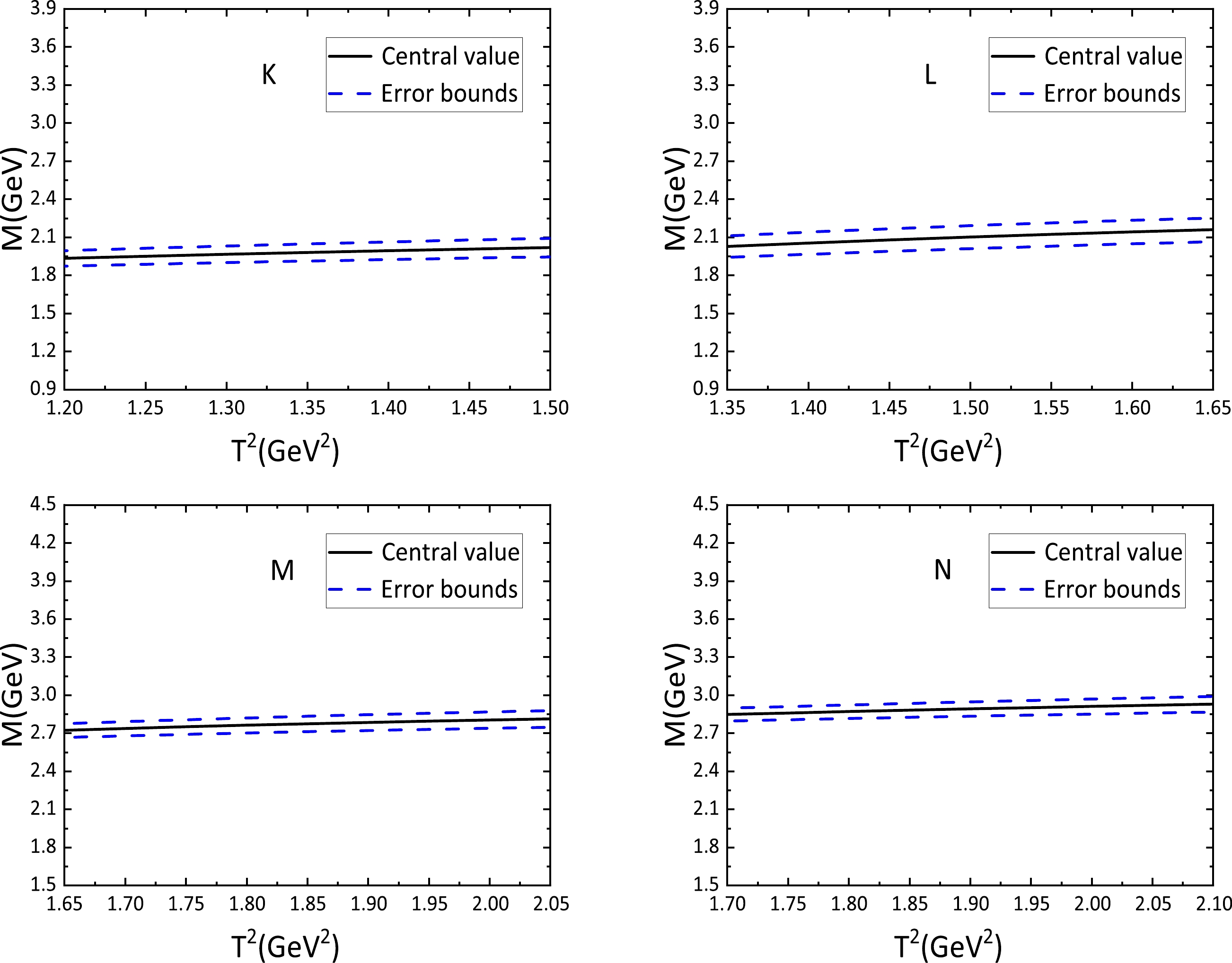
Figure 4. (color online) Masses with variations of the Borel parameters
$ T^2 $ , where K, L, M, and N denote the$ Y^1_{qq\bar{q}\bar{q}} $ ,$ Y^2_{qq\bar{q}\bar{q}} $ ,$ Y^3_{qq\bar{q}\bar{q}} $ and$ Y^4_{qq\bar{q}\bar{q}} $ P-wave (with partial derivatives) fully-light vector tetraquark states, respectively.Given that the currents
$ J_{\alpha} $ with same quantum numbers could mix with each other under renormalization, we introduce the mixing matrixes U to obtain the diagonal currents,$ J_{\alpha}^{\prime }=UJ_{\alpha} $ , which couple potentially to (more) physical states, as the physical states have several Fock components. The matrixes U can be determined by directly calculating anomalous dimensions of all the currents. It is difficult to obtain a diagonal current, because it is a special superposition of several non-trial currents that match with all the considerable Fock states. For the vector tetraquark state$ ss\bar{s}\bar{s} $ , if we want to obtain a more physical state, we have to account for the mixing effects of currents$ J^1_{\mu,ss\bar{s}\bar{s}} $ ,$ J^2_{\mu,ss\bar{s}\bar{s}} $ ,$ J^3_{\mu,ss\bar{s}\bar{s}} $ , and$ J^4_{\mu,ss\bar{s}\bar{s}} $ at least, and introduce three mixing angles, namely θ,$ \theta_{12} $ , and$ \theta_{34} $ ,$ \begin{aligned}[b] J_{\mu,ss\bar{s}\bar{s}}=&\cos\theta \left( \cos\theta_{12} J^1_{\mu,ss\bar{s}\bar{s}}+\sin\theta_{12} J^2_{\mu,ss\bar{s}\bar{s}}\right)\\&+\sin\theta \left( \cos\theta_{34} J^3_{\mu,ss\bar{s}\bar{s}}+\sin\theta_{34} J^4_{\mu,ss\bar{s}\bar{s}}\right) , \end{aligned} $

(28) Currents
$ J^1_{\mu,ss\bar{s}\bar{s}} $ ,$ J^2_{\mu,ss\bar{s}\bar{s}} $ ,$ J^3_{\mu,ss\bar{s}\bar{s}} $ , and$ J^4_{\mu,ss\bar{s}\bar{s}} $ may potentially couple to four different tetraquark states or a tetraquark state with four different Fock components. Without further exploring the mixing effects and strong decays in combination with precise experimental data, we cannot assign$ Y(2175)/\phi(2170) $ ,$ X(2240) $ , and$ X(2400) $ in a rigorous manner. At the present time, we just assign those exotic states tentatively and approximately. According to BESIII and BaBar data,$ Y(2175)/\phi(2170) $ and$ X(2240) $ are two different states [7, 10], and their valence quark constituents are favored to be$ ss\bar{s}\bar{s} $ and$ qs\bar{q}\bar{s} $ , respectively. The mixing effects between currents$ J^1_{\mu,ss\bar{s}\bar{s}} $ and$ J^2_{\mu,qs\bar{q}\bar{s}} $ are expected to be small; thus, the proposed assignments make sense. We expect that these vector tetraquark states can be experimentally verified in the future and the predictions can be confronted with experimental data from BESIII, LHCb, Belle II, etc. -
In this study, we construct fully-light vector/tensor four-quark currents and introduce an explicit P-wave between the diquark and antidiquark pairs. We analyze the contributions of the vacuum condensates up to dimension 11 in the operator product expansion and obtain the QCD sum rules for the masses and pole residues of the vector tetraquark states. For one of the
$ ss\bar{s}\bar{s} $ structures, the predicted mass$ M = 2.16\pm0.14\,{\rm{GeV}} $ is in great agreement with the experimental value of$ Y(2175)/\phi(2170) $ from the BaBar/BESIII/Belle collaborations, which supports assigning$ Y(2175)/\phi(2170) $ as the$ C\gamma_\alpha\otimes\stackrel{\leftrightarrow}{\partial}_\mu\otimes\gamma_\alpha C $ -type (or$ C\gamma_\alpha\otimes\stackrel{\leftrightarrow}D_\mu\otimes\gamma^\alpha C $ -type) fully-strange vector tetraquark state with an explicit P-wave. The$C\gamma_\mu\otimes \stackrel{\leftrightarrow}{\partial}_\alpha \otimes \gamma^\alpha C + $ $ C\gamma^\alpha \otimes\stackrel{\leftrightarrow}{\partial}_\alpha \otimes\gamma_\mu$ (or$ C\gamma_\mu\otimes \stackrel{\leftrightarrow}D_\alpha \otimes\gamma^\alpha C + C\gamma^\alpha \otimes\stackrel{\leftrightarrow}D_\alpha \otimes\gamma_\mu $ ) type$ qs\bar{q}\bar{s} $ and$ ss\bar{s}\bar{s} $ vector tetraquark states have masses compatible with the experimental values of$ X(2240) $ and$ X(2400) $ , respectively, in the region from$ 2.20 $ to$2.40~{\rm{GeV}}$ from the BaBar/BESIII collaborations. All in all, we predict that the central values of the masses of the vector$ ss\bar{s}\bar{s} $ tetraquark states with an explicit P-wave lie at the region$ 2.16-3.13\,{\rm{GeV}} $ (or$ 2.16-3.16\,{\rm{GeV}} $ ). We also obtain masses and pole residues of the$ sq\bar{s}\bar{q} $ and$ qq\bar{q}\bar{q} $ vector tetraquark states and expect that these fully-light vector tetraquark states can be observed in the future. -
The analytical expressions of the QCD spectral densities for the P-wave fully-light vector tetraquark states in the case of the partial derivatives are as follows:
$ \begin{aligned}[b]\\ \rho^1_{ss\bar{s}\bar{s}}(s)=\;& \frac{31s^5}{806400\pi^6}+\frac{s^3\,m_s\langle\bar{s}s\rangle}{40\pi^4} +\frac{s^3}{768\pi^4}\langle\frac{\alpha_{s}GG}{\pi}\rangle -\frac{25s^2\,m_s\langle\bar{s}g_{s}\sigma Gs\rangle}{576\pi^4} +\frac{s m_s\langle\bar{s}s\rangle}{9\pi^2}\langle\frac{\alpha_{s}GG}{\pi}\rangle \\ &+\frac{7s\langle\bar{s}s\rangle \langle\bar{s}g_{s}\sigma Gs\rangle}{9\pi^2} -\frac{7\langle\bar{s}s\rangle^2}{18}\langle\frac{\alpha_{s}GG}{\pi}\rangle -\frac{5\langle\bar{s}g_{s}\sigma Gs\rangle^2}{12\pi^2} -\frac{142m_s\langle\bar{s}s\rangle^2\langle\bar{s}g_{s}\sigma Gs\rangle}{27}\delta(s) \, , \end{aligned}\tag{A1} $ 
$ \begin{aligned}[b] \rho^2_{ss\bar{s}\bar{s}}(s)=\;& \frac{s^5}{23040\pi^6}+\frac{s^3\,m_s\langle\bar{s}s\rangle}{24\pi^4} +\frac{49s^3}{92160\pi^4}\langle\frac{\alpha_{s}GG}{\pi}\rangle -\frac{109s^2\,m_s\langle\bar{s}g_{s}\sigma Gs\rangle}{1152\pi^4}-\frac{s^2\langle\bar{s}s\rangle^2}{9\pi^2} +\frac{s m_s\langle\bar{s}s\rangle}{1728\pi^2}\langle\frac{\alpha_{s}GG}{\pi}\rangle \\& +\frac{17s\langle\bar{s}s\rangle \langle\bar{s}g_{s}\sigma Gs\rangle}{18\pi^2} -\frac{\langle\bar{s}s\rangle^2}{9}\langle\frac{\alpha_{s}GG}{\pi}\rangle -\frac{13\langle\bar{s}g_{s}\sigma Gs\rangle^2}{48\pi^2} -\frac{25m_s\langle\bar{s}s\rangle^2\langle\bar{s}g_{s}\sigma Gs\rangle}{9}\delta(s) \, , \end{aligned}\tag{A2} $

$ \rho^3_{ss\bar{s}\bar{s}}(s)= \frac{53s^5}{201600\pi^6}+\frac{3s^3\,m_s\langle\bar{s}s\rangle}{10\pi^4} +\frac{s^3}{192\pi^4}\langle\frac{\alpha_{s}GG}{\pi}\rangle -\frac{35s^2\,m_s\langle\bar{s}g_{s}\sigma Gs\rangle}{288\pi^4} -\frac{s m_s\langle\bar{s}s\rangle}{54\pi^2}\langle\frac{\alpha_{s}GG}{\pi}\rangle -\frac{128m_s\langle\bar{s}s\rangle^2\langle\bar{s}g_{s}\sigma Gs\rangle}{3}\delta(s) \, , \tag{A3} $

$ \begin{aligned}[b] \rho^4_{ss\bar{s}\bar{s}}(s)=\;& \frac{s^5}{20160\pi^6}+\frac{3s^3\,m_s\langle\bar{s}s\rangle}{40\pi^4} +\frac{s^3}{23040\pi^4}\langle\frac{\alpha_{s}GG}{\pi}\rangle -\frac{5s^2\,m_s\langle\bar{s}g_{s}\sigma Gs\rangle}{128\pi^4} +\frac{19s m_s\langle\bar{s}s\rangle}{864\pi^2}\langle\frac{\alpha_{s}GG}{\pi}\rangle +\frac{s\langle\bar{s}s\rangle \langle\bar{s}g_{s}\sigma Gs\rangle}{3\pi^2} \\ &-\frac{\langle\bar{s}s\rangle^2}{2}\langle\frac{\alpha_{s}GG}{\pi}\rangle -\frac{\langle\bar{s}g_{s}\sigma Gs\rangle^2}{2\pi^2} -\frac{146m_s\langle\bar{s}s\rangle^2\langle\bar{s}g_{s}\sigma Gs\rangle}{9}\delta(s) \, , \end{aligned}\tag{A4} $

$ \begin{aligned}[b] \rho^1_{qs\bar{q}\bar{s}}(s)=\;& \frac{31s^5}{3225600\pi^6}+\frac{s^3\,m_s(5\langle\bar{s}s\rangle-2\langle\bar{q}q\rangle)}{960\pi^4} +\frac{s^3}{3072\pi^4}\langle\frac{\alpha_{s}GG}{\pi}\rangle\\ & -\frac{s^2\,m_s(18\langle\bar{q}g_{s}\sigma Gq\rangle+7\langle\bar{s}g_{s}\sigma Gs\rangle)}{4608\pi^4}+\frac{s\,m_s(13\langle\bar{q}q\rangle+11\langle\bar{s}s\rangle)}{1728\pi^2}\langle\frac{\alpha_{s}GG}{\pi}\rangle \\ & +\frac{7s(\langle\bar{s}s\rangle \langle\bar{q}g_{s}\sigma G q\rangle +\langle\bar{q}q\rangle \langle\bar{s}g_{s}\sigma Gs\rangle)}{72\pi^2}-\frac{7\langle\bar{q}q\rangle\langle\bar{s}s\rangle}{72}\langle\frac{\alpha_{s}GG}{\pi}\rangle -\frac{5\langle\bar{q}g_{s}\sigma Gq\rangle\langle\bar{s}g_{s}\sigma Gs\rangle}{48\pi^2} \\ &-\frac{m_s(48\langle\bar{q}q\rangle^2\langle\bar{s}g_{s}\sigma Gs\rangle-12\langle\bar{s}s\rangle^2\langle\bar{q}g_{s}\sigma Gq\rangle+48\langle\bar{q}q\rangle\langle\bar{s}s\rangle\langle\bar{q}g_{s}\sigma Gq\rangle-13\langle\bar{q}q\rangle\langle\bar{s}s\rangle\langle\bar{s}g_{s}\sigma Gs\rangle)}{108}\delta(s) \, , \\ \end{aligned}\tag{A5} $

$ \begin{aligned}[b] \rho^2_{qs\bar{q}\bar{s}}(s)=\;& \frac{s^5}{92160\pi^6}+\frac{s^3\,m_s(3\langle\bar{s}s\rangle-\langle\bar{q}q\rangle)}{384\pi^4} +\frac{49s^3}{368640\pi^4}\langle\frac{\alpha_{s}GG}{\pi}\rangle \\ &-\frac{s^2\,m_s(41\langle\bar{q}g_{q}\sigma Gs\rangle+68\langle\bar{s}g_{s}\sigma Gs\rangle)}{9216\pi^4}-\frac{s^2\langle\bar{q}q\rangle\langle\bar{s}s\rangle}{36\pi^2} +\frac{s m_s(10\langle\bar{q}q\rangle-9\langle\bar{s}s\rangle)}{13824\pi^2}\langle\frac{\alpha_{s}GG}{\pi}\rangle \\ &+\frac{17s(\langle\bar{s}s\rangle \langle\bar{q}g_{s}\sigma Gq\rangle+\langle\bar{q}q\rangle \langle\bar{s}g_{s}\sigma Gs\rangle)}{144\pi^2} -\frac{\langle\bar{q}q\rangle\langle\bar{s}s\rangle}{36}\langle\frac{\alpha_{s}GG}{\pi}\rangle -\frac{13\langle\bar{q}g_{s}\sigma Gq\rangle\langle\bar{s}g_{s}\sigma Gs\rangle}{192\pi^2} \\ & -\frac{m_s(24\langle\bar{q}q\rangle^2\langle\bar{s}g_{s}\sigma Gs\rangle-10\langle\bar{s}s\rangle^2\langle\bar{q}g_{s}\sigma Gq\rangle+24\langle\bar{q}q\rangle\langle\bar{s}s\rangle\langle\bar{q}g_{s}\sigma Gq\rangle-13\langle\bar{q}q\rangle\langle\bar{s}s\rangle\langle\bar{s}g_{s}\sigma Gs\rangle)}{72}\delta(s) \, , \\ \end{aligned}\tag{A6} $

$ \begin{aligned}[b] \rho^3_{qs\bar{q}\bar{s}}(s)=\;& \frac{53s^5}{806400\pi^6}+\frac{3s^3\,m_s\langle\bar{s}s\rangle}{80\pi^4} +\frac{s^3}{768\pi^4}\langle\frac{\alpha_{s}GG}{\pi}\rangle -\frac{35s^2\,m_s\langle\bar{s}g_{s}\sigma Gs\rangle}{2304\pi^4} \\ &-\frac{s m_s\langle\bar{s}s\rangle}{432\pi^2}\langle\frac{\alpha_{s}GG}{\pi}\rangle -\frac{8m_s(\langle\bar{q}q\rangle^2\langle\bar{s}g_{s}\sigma Gs\rangle+\langle\bar{q}q\rangle\langle\bar{s}s\rangle\langle\bar{q}g_{s}\sigma Gq\rangle)}{3}\delta(s) \, , \end{aligned}\tag{A7} $

$ \begin{aligned}[b] \rho^4_{qs\bar{q}\bar{s}}(s)=\;& \frac{s^5}{80640\pi^6}+\frac{s^3\,m_s(2\langle\bar{q}q\rangle+7\langle\bar{s}s\rangle)}{960\pi^4} +\frac{s^3}{92160\pi^4}\langle\frac{\alpha_{s}GG}{\pi}\rangle -\frac{5s^2\,m_s\langle\bar{s}g_{s}\sigma Gs\rangle}{1024\pi^4} \\ &+\frac{s m_s(11\langle\bar{q}q\rangle+27\langle\bar{s}s\rangle)}{13824\pi^2}\langle\frac{\alpha_{s}GG}{\pi}\rangle +\frac{s(\langle\bar{s}s\rangle \langle\bar{q}g_{s}\sigma Gq\rangle+ \langle\bar{q}q\rangle\langle\bar{s}g_{s}\sigma Gs\rangle)}{24\pi^2} \\ &-\frac{\langle\bar{q}q\rangle\langle\bar{s}s\rangle}{8}\langle\frac{\alpha_{s}GG}{\pi}\rangle -\frac{\langle\bar{q}g_{s}\sigma Gq\rangle\langle\bar{s}g_{s}\sigma Gs\rangle}{8\pi^2}\\ & -\frac{m_s(192\langle\bar{q}q\rangle^2\langle\bar{s}g_{s}\sigma Gs\rangle+22\langle\bar{s}s\rangle^2\langle\bar{q}g_{s}\sigma Gq\rangle+192\langle\bar{q}q\rangle\langle\bar{s}s\rangle\langle\bar{q}g_{s}\sigma Gq\rangle+32\langle\bar{q}q\rangle\langle\bar{s}s\rangle\langle\bar{s}g_{s}\sigma Gs\rangle)}{216}\delta(s) \, ,\\ \end{aligned}\tag{A8} $

$ \begin{aligned}[b] \rho^5_{qs\bar{q}\bar{s}}(s)=\;& \frac{s^5}{691600\pi^6}+\frac{s^3\,m_s(2\langle\bar{q}q\rangle+\langle\bar{s}s\rangle)}{960\pi^4} +\frac{s^3}{46080\pi^4}\langle\frac{\alpha_{s}GG}{\pi}\rangle -\frac{7s^2\,m_s\langle\bar{s}g_{s}\sigma Gs\rangle}{18432\pi^4} \\ &+\frac{s m_s(8\langle\bar{q}q\rangle+3\langle\bar{s}s\rangle)}{6912\pi^2}\langle\frac{\alpha_{s}GG}{\pi}\rangle +\frac{s(\langle\bar{s}s\rangle \langle\bar{q}g_{s}\sigma Gq\rangle+ \langle\bar{q}q\rangle\langle\bar{s}g_{s}\sigma Gs\rangle)}{24\pi^2} \\ &-\frac{29\langle\bar{q}q\rangle\langle\bar{s}s\rangle}{576}\langle\frac{\alpha_{s}GG}{\pi}\rangle -\frac{\langle\bar{q}g_{s}\sigma Gq\rangle\langle\bar{s}g_{s}\sigma Gs\rangle}{16\pi^2}\\ & -\frac{m_s(24\langle\bar{q}q\rangle^2\langle\bar{s}g_{s}\sigma Gs\rangle-12\langle\bar{s}s\rangle^2\langle\bar{q}g_{s}\sigma Gq\rangle+24\langle\bar{q}q\rangle\langle\bar{s}s\rangle\langle\bar{q}g_{s}\sigma Gq\rangle-13\langle\bar{q}q\rangle\langle\bar{s}s\rangle\langle\bar{s}g_{s}\sigma Gs\rangle)}{216}\delta(s) \, ,\\ \end{aligned}\tag{A9} $

$ \begin{aligned}[b] \rho^6_{qs\bar{q}\bar{s}}(s)=\;& \frac{19s^5}{38707200\pi^6}+\frac{s^3\,m_s(9\langle\bar{s}s\rangle-5\langle\bar{q}q\rangle)}{11520\pi^4} +\frac{7s^3}{221184\pi^4}\langle\frac{\alpha_{s}GG}{\pi}\rangle -\frac{s^2\,m_s(467\langle\bar{q}g_{s}\sigma Gq\rangle-230\langle\bar{s}g_{s}\sigma Gs\rangle)}{110592\pi^4} \\ &+\frac{5s^2\langle\bar{q}q\rangle\langle\bar{s}s\rangle}{216\pi^2}-\frac{s m_s(227\langle\bar{q}q\rangle-20\langle\bar{s}s\rangle)}{41472\pi^2}\langle\frac{\alpha_{s}GG}{\pi}\rangle \\ &-\frac{s(\langle\bar{q}q\rangle \langle\bar{q}g_{s}\sigma Gq\rangle+\langle\bar{s}s\rangle \langle\bar{s}g_{s}\sigma Gs\rangle+353\langle\bar{s}s\rangle \langle\bar{q}g_{s}\sigma Gq\rangle+ 353\langle\bar{q}q\rangle\langle\bar{s}g_{s}\sigma Gs\rangle)}{5184\pi^2} \\ &+\frac{\langle\bar{q}q\rangle\langle\bar{s}s\rangle}{24}\langle\frac{\alpha_{s}GG}{\pi}\rangle -\frac{(\langle\bar{q}g_{s}\sigma Gq\rangle^2+\langle\bar{s}g_{s}\sigma Gs\rangle^2-82\langle\bar{q}g_{s}\sigma Gq\rangle\langle\bar{s}g_{s}\sigma Gs\rangle)}{1536\pi^2}\\ & +\frac{m_s(48\langle\bar{q}q\rangle^2\langle\bar{s}g_{s}\sigma Gs\rangle-17\langle\bar{s}s\rangle^2\langle\bar{q}g_{s}\sigma Gq\rangle+47\langle\bar{q}q\rangle\langle\bar{s}s\rangle\langle\bar{q}g_{s}\sigma Gq\rangle-25\langle\bar{q}q\rangle\langle\bar{s}s\rangle\langle\bar{s}g_{s}\sigma Gs\rangle)}{216}\delta(s)\, ,\\ \end{aligned}\tag{A10} $

$ \rho^1_{qq\bar{q}\bar{q}}(s)= \frac{31s^5}{806400\pi^6} +\frac{s^3}{768\pi^4}\langle\frac{\alpha_{s}GG}{\pi}\rangle+\frac{7s\langle\bar{q}q\rangle \langle\bar{q}g_{s}\sigma Gq\rangle}{9\pi^2} -\frac{7\langle\bar{q}q\rangle^2}{18}\langle\frac{\alpha_{s}GG}{\pi}\rangle -\frac{5\langle\bar{q}g_{s}\sigma Gq\rangle^2}{12\pi^2} \, , \tag{A11} $

$ \rho^2_{qq\bar{q}\bar{q}}(s)= \frac{s^5}{23040\pi^6} +\frac{49s^3}{92160\pi^4}\langle\frac{\alpha_{s}GG}{\pi}\rangle-\frac{s^2\langle\bar{q}q\rangle^2}{9\pi^2} +\frac{17s\langle\bar{q}q\rangle \langle\bar{q}g_{s}\sigma Gq\rangle}{18\pi^2}-\frac{\langle\bar{q}q\rangle^2}{9}\langle\frac{\alpha_{s}GG}{\pi}\rangle -\frac{13\langle\bar{q}g_{s}\sigma Gq\rangle^2}{48\pi^2} \, , \tag{A12} $

$ \rho^3_{qq\bar{q}\bar{q}}(s)= \frac{53s^5}{201600\pi^6} +\frac{s^3}{192\pi^4}\langle\frac{\alpha_{s}GG}{\pi}\rangle \, , \tag{A13} $

$ \rho^4_{qq\bar{q}\bar{q}}(s)= \frac{s^5}{20160\pi^6} +\frac{s^3}{23040\pi^4}\langle\frac{\alpha_{s}GG}{\pi}\rangle+\frac{s\langle\bar{q}q\rangle \langle\bar{q}g_{s}\sigma Gq\rangle}{3\pi^2} -\frac{\langle\bar{q}q\rangle^2}{2}\langle\frac{\alpha_{s}GG}{\pi}\rangle -\frac{\langle\bar{q}g_{s}\sigma Gq\rangle^2}{2\pi^2} \, . \tag{A14} $

With simple replacements
$ \begin{aligned}[b] \rho^{1/2/3/4}_{ss\bar{s}\bar{s}}(s)\to\;&\rho^{1/2/3/4}_{ss\bar{s}\bar{s}}(s)+\tilde{\rho}^{1/2/3/4}_{ss\bar{s}\bar{s}}(s)\, , \\ \rho^{1/2/3/4/5/6}_{qs\bar{q}\bar{s}}(s)\to\;&\rho^{1/2/3/4/5/6}_{qs\bar{q}\bar{s}}(s)+\tilde{\rho}^{1/2/3/4/5/6}_{qs\bar{q}\bar{s}}(s)\, , \\ \rho^{1/2/3/4}_{qq\bar{q}\bar{q}}(s)\to\;&\rho^{1/2/3/4}_{qq\bar{q}\bar{q}}(s)+\tilde{\rho}^{1/2/3/4}_{qq\bar{q}\bar{q}}(s)\, , \end{aligned}\tag{A15} $

we obtain the corresponding QCD spectral densities for the currents with covariant derivatives, with additional terms
$ \tilde{\rho}^1_{ss\bar{s}\bar{s}}(s)=0\, , \tag{A16}$

$ \begin{aligned}[b] \tilde{\rho}^2_{ss\bar{s}\bar{s}}(s)=\;&-\frac{77s^3}{184320\pi^4}\langle\frac{\alpha_{s}GG}{\pi}\rangle +\frac{253 s m_s\langle\bar{s}s\rangle}{6912\pi^2}\langle\frac{\alpha_{s}GG}{\pi}\rangle\\& -\frac{11\langle\bar{s}s\rangle^2}{96}\langle\frac{\alpha_{s}GG}{\pi}\rangle \, , \end{aligned}\tag{A17} $

$ \tilde{\rho}^3_{ss\bar{s}\bar{s}}(s)=0\, , \tag{A18} $

$ \begin{aligned}[b] \tilde{\rho}^4_{ss\bar{s}\bar{s}}(s)=\;&-\frac{51s^3}{61440\pi^4}\langle\frac{\alpha_{s}GG}{\pi}\rangle +\frac{7s^2\,m_s\langle\bar{s}g_{s}\sigma Gs\rangle}{2304\pi^4}\\& +\frac{719s m_s\langle\bar{s}s\rangle}{6912\pi^2}\langle\frac{\alpha_{s}GG}{\pi}\rangle \\ & +\frac{5s\langle\bar{s}s\rangle \langle\bar{s}g_{s}\sigma Gs\rangle}{864\pi^2} -\frac{\langle\bar{s}g_{s}\sigma Gs\rangle^2}{384\pi^2}\\& -\frac{m_s\langle\bar{s}s\rangle^2\langle\bar{s}g_{s}\sigma Gs\rangle}{108}\delta(s) \, , \end{aligned}\tag{A19} $

$ \tilde{\rho}^1_{qs\bar{q}\bar{s}}(s)=0\, , \tag{A20}$

$ \begin{aligned}[b] \tilde{\rho}^2_{qs\bar{q}\bar{s}}(s)=\;&-\frac{77s^3}{737280\pi^4}\langle\frac{\alpha_{s}GG}{\pi}\rangle \\&+\frac{77 s m_s(2\langle\bar{q}q\rangle-\langle\bar{s}s\rangle)}{13824\pi^2}\langle\frac{\alpha_{s}GG}{\pi}\rangle \\&-\frac{11\langle\bar{s}s\rangle^2}{384}\langle\frac{\alpha_{s}GG}{\pi}\rangle \, , \end{aligned}\tag{A21} $

$ \tilde{\rho}^3_{qs\bar{q}\bar{s}}(s)=0\, , \tag{A22}$

$ \begin{aligned}[b] \tilde{\rho}^4_{qs\bar{q}\bar{s}}(s)=\;&-\frac{51s^3}{245760\pi^4}\langle\frac{\alpha_{s}GG}{\pi}\rangle \\& +\frac{sm_s(\langle\bar{q}q\rangle-153\langle\bar{s}s\rangle)}{13824\pi^2}\langle\frac{\alpha_{s}GG}{\pi}\rangle \\ & +\frac{5s\langle\bar{q}q\rangle \langle\bar{s}g_{s}\sigma Gs\rangle}{3456\pi^2} \\&-\frac{\langle\bar{q}g_{q}\sigma Gs\rangle\langle\bar{s}g_{s}\sigma Gs\rangle}{1536\pi^2}\\& -\frac{m_s\langle\bar{q}q\rangle \langle\bar{s}s\rangle \langle\bar{s}g_{s}\sigma Gs\rangle}{864}\delta(s) \, , \end{aligned}\tag{A23} $

$ \tilde{\rho}^5_{qs\bar{q}\bar{s}}(s)=0\, , \tag{A24} $

$ \begin{aligned}[b] \tilde{\rho}^6_{qs\bar{q}\bar{s}}(s)=\;&\frac{7s^3}{2211840\pi^4}\langle\frac{\alpha_{s}GG}{\pi}\rangle +\frac{7s^2\,m_s \langle\bar{q}g_{s}\sigma Gq\rangle}{36864\pi^4}-\frac{sm_s(7\langle\bar{q}q\rangle-4\langle\bar{s}s\rangle)}{20736\pi^2}\langle\frac{\alpha_{s}GG}{\pi}\rangle \\ &-\frac{(5\langle\bar{s}s\rangle \langle\bar{q}g_{s}\sigma Gq\rangle+ 5\langle\bar{q}q\rangle\langle\bar{s}g_{s}\sigma Gs\rangle)}{3456\pi^2}+\frac{7\langle\bar{q}q\rangle\langle\bar{s}s\rangle}{6912}\langle\frac{\alpha_{s}GG}{\pi}\rangle +\frac{\langle\bar{q}g_{s}\sigma Gq\rangle\langle\bar{s}g_{s}\sigma Gs\rangle}{768\pi^2}\\ & +\frac{m_s(2\langle\bar{q}q\rangle^2\langle\bar{s}g_{s}\sigma Gs\rangle-\langle\bar{s}s\rangle^2\langle\bar{q}g_{s}\sigma Gq\rangle+2\langle\bar{q}q\rangle\langle\bar{s}s\rangle\langle\bar{q}g_{s}\sigma Gq\rangle-\langle\bar{q}q\rangle\langle\bar{s}s\rangle\langle\bar{s}g_{s}\sigma Gs\rangle)}{2592}\delta(s)\, , \\ \end{aligned}\tag{A25} $ 
$ \tilde{\rho}^1_{qq\bar{q}\bar{q}}(s)=0\, , \tag{A26} $

$ \tilde{\rho}^2_{qq\bar{q}\bar{q}}(s)=-\frac{77s^3}{184320\pi^4}\langle\frac{\alpha_{s}GG}{\pi}\rangle -\frac{11\langle\bar{q}q\rangle^2}{96}\langle\frac{\alpha_{s}GG}{\pi}\rangle \, , \tag{A27} $

$ \tilde{\rho}^3_{qq\bar{q}\bar{q}}(s)=0\, , \tag{A28} $

$ \begin{aligned}[b] \tilde{\rho}^4_{qq\bar{q}\bar{q}}(s)=\;&-\frac{51s^3}{61440\pi^4}\langle\frac{\alpha_{s}GG}{\pi}\rangle +\frac{5s\langle\bar{q}q\rangle \langle\bar{q}g_{s}\sigma Gq\rangle}{864\pi^2} \\&-\frac{\langle\bar{q}g_{s}\sigma Gq\rangle^2}{384\pi^2} \, . \end{aligned}\tag{A29} $

Fully-light vector tetraquark states with explicit P-wave via QCD sum rules
- Received Date: 2023-10-07
- Available Online: 2024-03-15
Abstract: In this study, we apply the QCD sum rules to investigate the vector fully-light tetraquark states with an explicit P-wave between the diquark and antidiquark pairs. We observed that the


 DownLoad: