Elastic scattering based on energy-dependent relativistic Love-Franey model at energies between 20 and 800 MeV

I. INTRODUCTION

• I. INTRODUCTION
• II. FORMALISM
• III. RESULTS AND DISCUSSIONS
•      A Fitting procedures and results
•      B Proton-nucleus scattering results and discussions
• IV. SUMMARY
• ACKNOWLEDGMENT

The interaction between nucleons is very important in understanding the nuclear experiments and the properties of nuclei and neutron stars. However, the interaction between nucleons is still poorly understood, particularly at high densities. The main reason for this is that the interaction is not a directly observable quantity in experiments. The interaction between nucleons as residual interactions of the QCD cannot be solved via perturbation expansion. Therefore, the interaction between nucleons leads to the uncertainty of the symmetry energy. Considerable effort has been directed toward understanding the interaction between nucleons. The global Dirac phenomenological optical potentials, which describe the elastic proton scattering observables of $^{12}$C and $^{208}$Pb well for incident energies between 20 and 1040 MeV [1, 2], are powerful tools in understanding the interaction between nucleons. They have been widely used to extract the symmetry energy directly or indirectly [3, 4]. The relativistic impulse approximation (RIA) [5–7] can also be used to describe the elastic proton scattering observables. Theoretically, the symmetry energy can be extracted from the microscopic potentials of the RIA.

The original RIA with scalar and vector potentials can reproduce the analyzing power and spin-rotation parameter in proton-nucleus scattering for incident energies above 500 MeV [5, 8]. Because the direct and exchange parts of the t-matrix are not separated explicitly in the original RIA, the optical potential of the original RIA diverges at energies below 500 MeV [8]. By separating the direct and exchange parts of the t-matrix, it is found that the pion with pseudoscalar leads to the divergent optical potential. This can be cured by introducing the pion with pseudovector coupling, in a process known as the relativistic Love-Franey (RLF) model [6, 9,10]. The RLF model has been used to describe the elastic proton scattering observables successfully for incident energies of 135, 200, 300, and 400 MeV [6]. The shortcoming of the original RLF model is that the scattering observables were fitted separately at each energy. The separate fits of the scattering observables cannot reflect the energy-dependent trend of the scattering observables. This motivates the proposal of the energy-dependent RLF model [11, 12]. The energy-dependent RLF model has been used to fit empirical amplitudes successfully at incident energies of 50–200 MeV [13], 200–500 MeV [11], and 500–800 MeV [12]. It should be noted that these fits are separated from each other. In this work, we try to construct the energy-dependent RLF model over the laboratory energy range of 20 to 800 MeV within a unified fit.

The RLF model has been used to study both elastic proton-nucleus scattering [6, 7] and the (p, 2p) reaction [14]. The RLF model without Pauli blocking (PB) corrections cannot well describe the differential cross sections ${\rm d}\Omega/{\rm d}\sigma$, analyzing powers $A_y$, and spinrotation functions Q of elastic proton-nucleus scattering. With the PB corrections, the RLF model can describe ${\rm d}\Omega/{\rm d}\sigma$, $A_y$, and Q well [6, 7]. The RLF model is also helpful in understanding the in-medium effect. In-medium nucleon-nucleon (NN) cross sections, which are key inputs of various transport models, can be obtained from RLF. It has been recognized that the theoretical uncertainty in extracting the density dependence of the symmetry energy from data of heavy-ion reactions can be largely ascribed to the poor knowledge and premature treatment of the isospin-dependent in-medium NN cross sections [15, 16]. Although the NN cross section in free space is well-determined, the in-medium NN cross section is still model dependent [17–28]. Under the original RIA framework, the in-medium NN cross sections have been studied [24, 28]. However, no such work has been done in the framework of the RLF model. At a low nucleon kinetic energy, it would be interesting to study the in-medium NN cross sections with the RLF model. Additionally, the energy and density dependent symmetry potential of nuclear matter has been investigated with the original RIA and RLF models [24, 28, 29]. The energy and density dependence symmetry potential of the energy-dependent RLF model may have some differences from the results of the original RIA and RLF models.

The remainder of this paper is organized as follows. In Sec. II, we briefly introduce formulas and approaches used in this work. The formulas include the fits between RIA scattering amplitudes and the empirical amplitudes, as well as the elastic proton scattering observables of $^{208}$Pb. Results and discussions are presented in Sec. III. Finally, a summary is given in Sec. IV.

II. FORMALISM

• I. INTRODUCTION
• II. FORMALISM
• III. RESULTS AND DISCUSSIONS
•      A Fitting procedures and results
•      B Proton-nucleus scattering results and discussions
• IV. SUMMARY
• ACKNOWLEDGMENT

In order to obtain the on-shell NN matrix elements of RLF scattering amplitudes, one needs to transform the NN matrix elements of RLF scattering amplitudes into those of the non-relativistic NN scattering amplitudes. The relation between the matrix elements of the RLF scattering amplitudes and the matrix elements of the non-relativistic NN scattering amplitudes in the center-of-mass frame can be written as [5, 6, 9, 10, 13]

where $k_1\equiv (E_c,\mathbf{k}_c)$ and $k_2\equiv (E_c,-\mathbf{k}_c)$ are the incident 4-momenta in the center-of-mass frame. $\chi'$s represent the usual Pauli spinors. $k_c$ represents the momentum in the center of mass frame. The Dirac spinors are normalized ($\bar{u}u$=1). $\hat{f}_{cm}$ and $\hat{F}$ are the non-relativistic scattering matrix and scattering matrix of RLF respectively. $\hat{f}_{cm}$ contains five real and imaginary amplitudes [30]:

where a, b, c, d, and e are the non-relativistic real and imaginary amplitudes. The scattering matrix of RLF $\hat{F}$ also contains five real and imaginary amplitudes:

where i includes the scalar (S), vector (V), pseudoscalar (P), axial vector (A), and tensor (T). $F_S$, $F_V$, $F_P$, $F_A$, and $F_T$ are the relativistic amplitudes of RLF. The Dirac matrices of S, V, P, A, and T are $I_{4\times 4}$, $\gamma_\mu$, $\gamma_5$, $\gamma_5\gamma_\mu$, and $\sigma_{\mu\nu}$ respectively. With these Dirac matrices and Eq. (1), the relation between the non-relativistic amplitudes and the relativistic amplitudes is obtained as follows [5, 9, 10, 13]:

The $O_{5\times5}$ matrix is written as [10, 13]

with

where θ represents the scattering angle in the two-body center-of-mass, and M represents the free nucleon mass. Now, the relation between the matrix elements of the RLF scattering amplitudes and the matrix elements of the non-relativistic NN scattering amplitudes is clear. For comparison with the empirical amplitudes, the relativistic amplitudes $F_i(s,t,u)$ need to be solved. The $F_i(s,t,u)$ contains direct and exchange contributions:

with

where N represents the number of mesons in this work, $C_{i(j),i}$ is the Fierz matrix [6, 9, 31], $T_j$ is the isospin of the jth meson, and $T_{NN}$ is the total isospin of the two-nucleon state. When $T_{NN}=1$, $\langle\mathbf{\tau}_1\cdot\mathbf{\tau}_2\rangle^{T_j}=1$ for both $T_j=0$ and $T_j=1$. When $T_{NN}=0$, $\langle\mathbf{\tau}_1\cdot\mathbf{\tau}_2\rangle^{T_j}=1$ for $T_j=0$, and $\langle\mathbf{\tau}_1\cdot\mathbf{\tau}_2\rangle^{T_j}=-3$ for $T_j=1$. For instance, when $T_{NN}=0$, the scalar amplitudes are written as

where $f^j(E_c,|\mathbf{q}|)$ and $f^j(E_c,|\mathbf{Q}|)$ contain the real and imaginary parts. For instance:

where $g_j^2(E_c)$, $m_j$, and $\Lambda_j$ are the coupling constant, mass, and momentum cutoff of the jth real meson, respectively. $\bar{g}_j^2(E_c)$, $\bar{m}_j$, and$\bar{\Lambda}_j$ are the coupling constant, mass, and cutoff parameter of the jth imaginary meson, respectively. The direct momentum transfer $|\mathbf{q}|$ and the exchange momentum transfer $|\mathbf{Q}|$ are written as [9]

For a given projectile's kinetic energy $T_{\rm lab}$, the momentum and energy of the center of mass frame are $k_c=\dfrac{\sqrt{2MT_{\rm lab}}}{2}$ and $E_c=\sqrt{k_c^2+M^2}$, respectively. With these fitting formulas, the parameterization of the RLF model can be obtained. Then, the Dirac optical potential is generated with the fitting parameters of the RLF model.

The Dirac optical potential of the RLF model is the same as that of the original RIA model [6, 32, 33]:

where $p_{\rm lab}$ represents the laboratory momentum of incident nucleons. q and E represent the momentum transfer and collision energy, respectively. $|\Psi\rangle$ represents the A-particle ground state of the target nucleus.

In proton-nucleus scattering, the scattering process can be approximately treated as incident protons scattered by each of the nucleons in the target nucleus. Assuming the incident proton wave function as $U_0(\mathbf{r})$ and the relativistic Hartree wave function of the nucleus ground state as $U_0(\mathbf{r})$, the optical potential can act on the incident proton wave function and project into the coordinate space. In this work, we only list the formulas after Fourier transforms [33]:

where

with $t_D^L(q,E)\equiv ({\rm i} M^2/2E_ck_c)F_D^L({q})$ and $t_E^L(Q,E)\equiv ({\rm i}M^2/ 2E_ck_c)F_E^L({Q})$, respectively. The first term of the above equation represents the direct optical potential in the coordinate space:

and the second term of the above equation represents the exchange optical potential. With the local-density approximation, the exchange optical potential is written as

$j_0$ is a spherical Bessel function. The nuclear densities of Eqs. (13), (16), and (17) are defined as

The occupied states indicate that one sums over target protons for the density with pp amplitudes and over target neutrons for the density with pn amplitudes. The densities of target protons and neutrons can be obtained from relativistic mean field theory (RMF) [7, 33]. When the densities of target protons and neutrons predicted by various models are substituted into Eq. (18), the results are almost the same in p+$^{208}$ Pb elastic scattering. In the following sections, we take the densities predicted by the code of Ref. [33] as the input.

With above formulas, the Dirac optical potential can be obtained. For the spin-saturated nucleus, the Dirac optical potential only contains scalar, vector, and tensor terms. Because the tensor contribution is small, the tensor contribution has been neglected in the calculation. The Dirac optical potential is simplified as

For the laboratory energy near 200 MeV, the contribution of Pauli blocking (PB) plays an important role in the calculations. The modification of PB with a local-density approximation is [6, 13, 33]

Here, $\rho_B(\mathbf{r})$ represents the local baryon density of the target nuclus, and $\rho_0=0.1934~\rm fm^{-3}$.

With the Dirac optical potential, the Dirac equation of the projectile is written as

By solving the Dirac equation, i.e., Eq. (21), the scattering observables (the differential cross section ${\rm d}\sigma/{\rm d}\Omega$, analyzing power $A_y$, and spin rotation function Q) are determined. The detailed solution processes are presented in Ref. [33]. In this work, we concentrate on ${\rm d}\sigma/ {\rm d}\Omega$, $A_y$, and Q of p+$^{208}$Pb elastic scattering.

III. RESULTS AND DISCUSSIONS

• I. INTRODUCTION
• II. FORMALISM
• III. RESULTS AND DISCUSSIONS
•      A Fitting procedures and results
•      B Proton-nucleus scattering results and discussions
• IV. SUMMARY
• ACKNOWLEDGMENT

A Fitting procedures and results

• I. INTRODUCTION
• II. FORMALISM
• III. RESULTS AND DISCUSSIONS
•      A Fitting procedures and results
•      B Proton-nucleus scattering results and discussions
• IV. SUMMARY
• ACKNOWLEDGMENT

The RLF pp and pn scattering amplitudes are written as [9]

where the relativistic amplitudes $F_S$, $F_V$, $F_P$, and $F_A$ of pp and pn and the non-relativistic amplitudes a, b, c, d, and e of pp and pn are generated from Eq. (4). However, the non-relativistic amplitudes are no longer available on the on-line Scattering Analysis Interactive Dial-in (SAID) facility. The scattering observables are still available on SAID. There are several models available for computing the scattering observables on SAID. We choose the scattering observables obtained from the weighted fits (WF16) on SAID [34]. In contrast to previous studies [11–13], we fit 10 scattering observables of the weighted fits (WF16) rather than the real and imaginary amplitudes of pp and pn. These 10 scattering observables are written as [30]

These 10 scattering observables are the unpolarized differential cross section ($\rm\dfrac{d\sigma}{d\Omega}$), depolarization tensor for polarized beam (D), polarization transfer from beam to recoil particle (DT), polarization correlation for initially unpolarized particles $A_{yy}$, CKP, CKK, CPP, polarization of scattered particle (P), and triple scattering parameters A and R. α is a function of the angle:

where $\theta_{\rm lab}$ represents the laboratory scattering angle. Theoretically, the fitting quality with these 10 scattering observables of pp and pn should be as good as that in the previous case with the non-relativistic amplitudes of pp and pn.

The real isovector pseudoscalar (π), isoscalar vector (ω), and isovector vector (ρ) masses are fixed to their physical values $m_{\pi}=138$ MeV, $m_{\omega}=782$ MeV, and $m_{\rho}=$ 770 MeV, respectively. The remaining meson masses are set in accordance with Ref. [13]. Because the energy boundary between low energy and high energy is around 200 MeV, we first fit the scattering observables to obtain the initial coupling strengths of RLF. The initial coupling constant ${g}_0^2$ ($\bar{g}_0^2$) and the cutoff parameter Λ ($\bar{\Lambda}$) are obtained by fitting the scattering observables for $T_{\rm lab}=$ 200 MeV alone. In order to obtain the best fit to the scattering observables for $T_{\rm lab}=$ 200 MeV, the Levenberg-Marquadt method has been employed to minimize the value of $\chi^2$. $\chi^2$ is defined as follows:

where $\langle\chi_{\rm empirical}^2\rangle$ represents an angle-averaged value and is defined as

where $N_{\rm empirical}=35$ represents the number of angles per energy. For a single incident energy, the number of the data points is 700: 35 angles $\times$ 10 scattering observables $\times$ 2 pp and pn. As a result, the real (imaginary) initial coupling constant ${g}_0^2$ ($\bar{g}_0^2$), the real (imaginary) meson mass ${m}$ ($\bar{m}$), and the real (imaginary) cutoff parameter Λ ($\bar{\Lambda}$) are presented in Table 1. It should be noted that $\Lambda > m$ has been employed for a given meson.

Table 1

Table 1.  Parameter sets for the energy-dependent RLF over the laboratory energy range of 20 to 800 MeV. The masses m ($\bar{m}$) and cutoff parameters Λ ($\bar{\Lambda}$) are in MeV, whereas the remaining parameters are dimensionless.

Real parameters
Meson	Isospin	Coupling type	m	$g_0^2$	$a_1$	$a_2$	$a_3$	$a_4$	Λ
σ	0	Scalar (S)	600	−8.348	6.527$\times10^{-1}$	2.773	−2.741$\times10^{-2}$	−7.639	962.7
ω	0	Vector (V)	782	1.019$\times10^{1}$	−6.246$\times10^{-1}$	−1.400$\times10^{1}$	8.492$\times10^{-1}$	2.677$\times10^{1}$	1155
$t_0$	0	Tensor (T)	550	2.794$\times10^{-1}$	3.303	1.172$\times10^{1}$	−6.676$\times10^{-1}$	−3.008$\times10^{1}$	1945
$a_0$	0	Axial vector (A)	500	4.921$\times10^{-1}$	6.066	1.953$\times10^{1}$	−1.089	−5.133$\times10^{1}$	1597
η	0	Pseudoscalar (P)	950	1.180$\times10^{1}$	−1.694$\times10^{2}$	−1.350$\times10^{2}$	5.417	5.550$\times10^{2}$	957.3
δ	1	Scalar (S)	500	6.095$\times10^{-3}$	5.635$\times10^{-1}$	1.287	−6.040$\times10^{-2}$	−4.101	2945
ρ	1	Vector (V)	770	−1.667$\times10^{-1}$	9.420$\times10^{-5}$	1.644$\times10^{-1}$	−2.905$\times10^{-2}$	2.915$\times10^{-1}$	3001
$t_1$	1	Tensor (T)	600	−2.500$\times10^{-1}$	−1.893	−7.848	4.448$\times10^{-1}$	1.989$\times10^{1}$	1280
$a_1$	1	Axial vector (A)	650	−1.356	−4.678	−1.529$\times10^{1}$	8.102$\times10^{-1}$	4.146$\times10^{1}$	745.1
π	1	Pseudoscalar (P)	138	1.095$\times10^{1}$	−3.834$\times10^{-9}$	−4.889	4.005$\times10^{-1}$	1.082$\times10^{1}$	677.4
Imaginary parameters
Meson	Isospin	Coupling type	$\bar{m}$	$\bar{g}_0^2$	$a_1$	$a_2$	$a_3$	$a_4$	$\bar{\Lambda}$
σ	0	Scalar (S)	600	−2.849	−4.637	−1.475$\times10^{1}$	6.301$\times10^{-1}$	4.377$\times10^{1}$	800.0
ω	0	Vector (V)	700	4.405	4.825	2.077$\times10^{1}$	−9.616$\times10^{-1}$	−5.672 $\times10^{1}$	716.0
$t_0$	0	Tensor (T)	750	−9.457$\times10^{-1}$	−1.474	−7.535	4.140$\times10^{-1}$	1.914$\times10^{1}$	1340
$a_0$	0	Axial vector (A)	750	−2.198	−3.583	−1.374$\times10^{1}$	6.840$\times10^{-1}$	3.762$\times10^{1}$	1437
η	0	Pseudoscalar (P)	1000	1.420$\times10^{1}$	−1.619$\times10^{2}$	−2.011$\times10^{2}$	9.779	6.591$\times10^{2}$	2758
δ	1	Scalar (S)	650	3.094	1.593	2.945	1.614$\times10^{-2}$	−1.328$\times10^{1}$	751.9
ρ	1	Vector (V)	600	−2.421	−9.543$\times10^{-1}$	−3.644	9.074$\times10^{-2}$	1.292$\times10^{1}$	766.6
$t_1$	1	Tensor (T)	750	6.140$\times10^{-1}$	1.513	5.775	−3.011$\times10^{-1}$	−1.557$\times10^{1}$	1662
$a_1$	1	Axial vector (A)	1000	2.265	5.071	1.997$\times10^{1}$	−1.011	−5.450$\times10^{1}$	1233
π	1	Pseudoscalar (P)	500	−5.891	2.029$\times10^{1}$	2.363$\times10^{1}$	−9.593$\times10^{-1}$	−7.574$\times10^{1}$	1342

DownLoad: CSV

Show Table

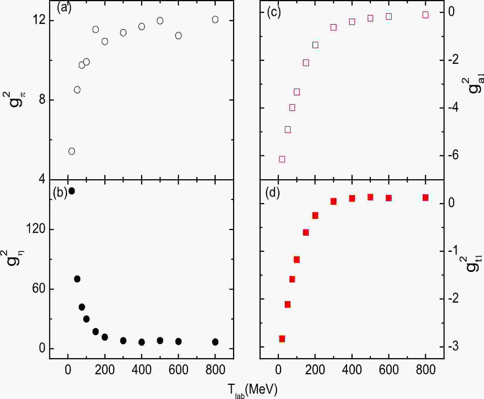
The energy-dependent RLF model has been used to fit the empirical NN data for separate incident energies (50–200 MeV [13], 200–500 MeV [11], and 500–800 MeV [12]). To relate these energy domains, we first fit the scattering observables of various energies ($T_{\rm lab}=$ 20, 50, 75, 100, 150, 200, 300, 400, 500, 600, and 800 MeV) separately with the same cutoff parameters and meson masses as 200 MeV. As shown in Fig. 1, we find that the coupling strengths, such as $g_{\pi}^2$, $g_{\eta}^2$, $g_{a1}^2$, and $g_{t1}^2$, approximately follow a logarithmic or parabolic curve opening to the right. Combining the linear and square terms [11, 12], the energy-dependent coupling strengths can be written as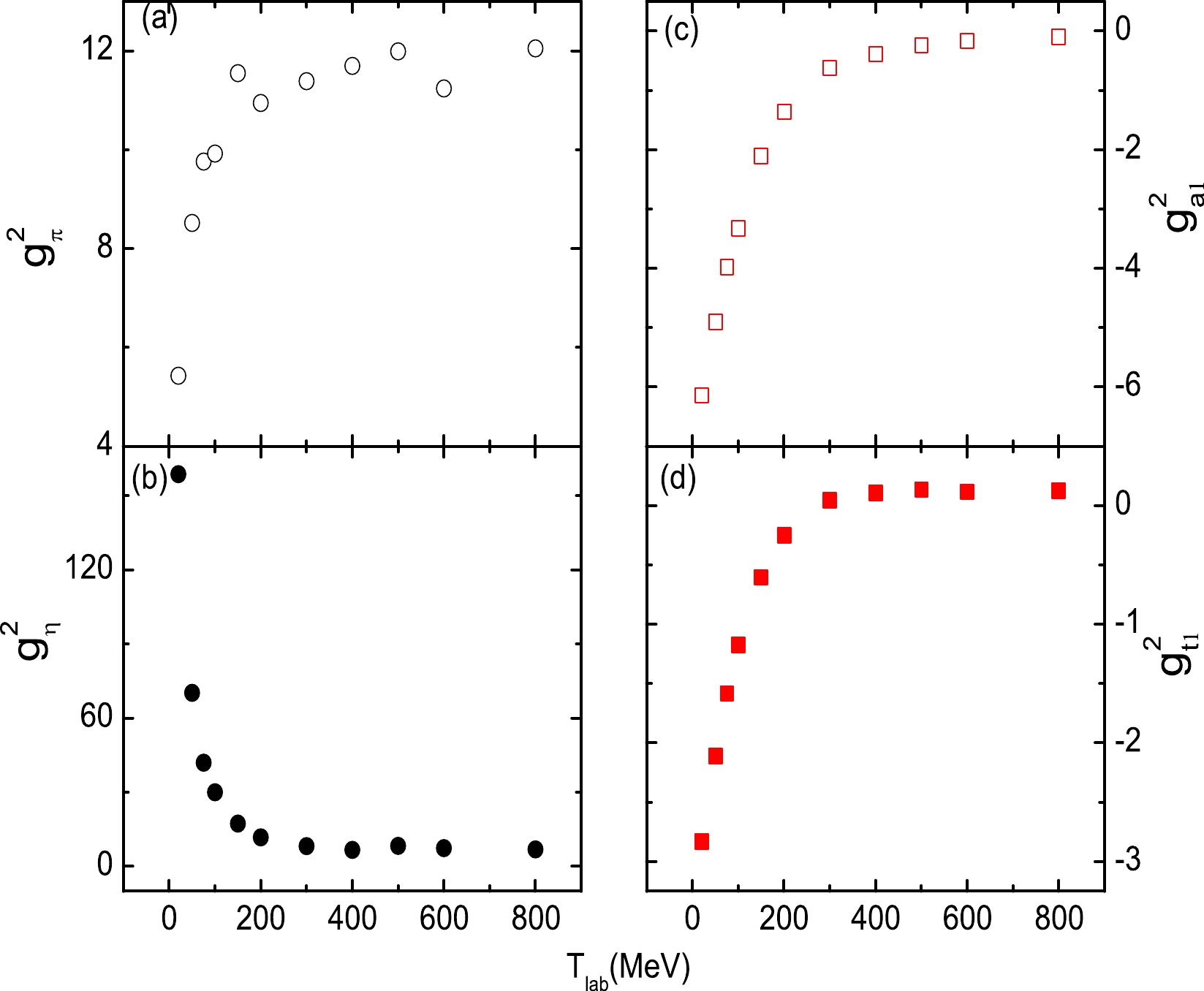

Figure 1

Figure 1.  (color online) The coupling constants ($g_{\pi}^2$, $g_{\eta}^2$, $g_{a1}^2$, and $g_{t1}^2$) as a function of the laboratory energies $T_{\rm lab}$. The coupling constants are obtained from separate fits with $T_{\rm lab}=$ 20, 50, 75, 100, 150, 200, 300, 400, 500, 600, and 800 MeV.

DownLoad: Full-Size Img PowerPoint

with $T_0=200$ MeV. This equation is also valid for the imaginary coupling strengths. When the incident energy is 200 MeV, the energy-dependent coupling strengths should equal the initial coupling strengths. The meson masses and cutoff parameters of RLF are assumed to be independent of the energy in this work.

For various incident energies, the initial coupling constant, the meson mass, and the cutoff parameter remain the same. However, the coupling constants ${g}_j^2(E_c)$ and $\bar{g}_j^2(E_c)$ change with respect to the incident energy. The parameters $a_1$, $a_2 a_3$, and $a_4$ of Eq. (27) are obtained by fitting the scattering observables for various incident energies ($T_{\rm lab}=$ 20, 50, 75, 100, 150, 200, 300, 400, 500, 600, and 800 MeV) uniformly. The number of the data points is 7700: 11 energies $\times$ 35 angles $\times$ 10 scattering observables $\times$ 2 pp and pn. The final results for $a_1$, $a_2 a_3$, and $a_4$ are presented in Table 1.

To illustrate the fitting quality, we show the unpolarized differential cross section ($\rm\frac{d\sigma}{d\Omega}$), depolarization tensor for the polarized beam (D), polarization transfer from beam to recoil particle (DT), polarization correlation for initially unpolarized particles ($A_{yy}$), and polarization of scattered particles (P) of pp and pp at $T_{\rm lab}=$ 20, 100, 200, 400, and 800 MeV in Figs. 2–6. At $T_{\rm lab}=$ 200 MeV, as shown in Fig. 4, because the scattering observables of $T_{\rm lab}=$ 200 MeV are fitted alone, the scattering observables are described well for both np and pp. As the Coulomb corrections dominate the empirical pp scattering observables of forward and backward angles, the Coulomb corrections are included in the pp scattering observables in this work. The Coulomb corrections are obtained by subtracting the $T_{NN} = 1$ amplitudes of SAID from the pp amplitudes of SAID.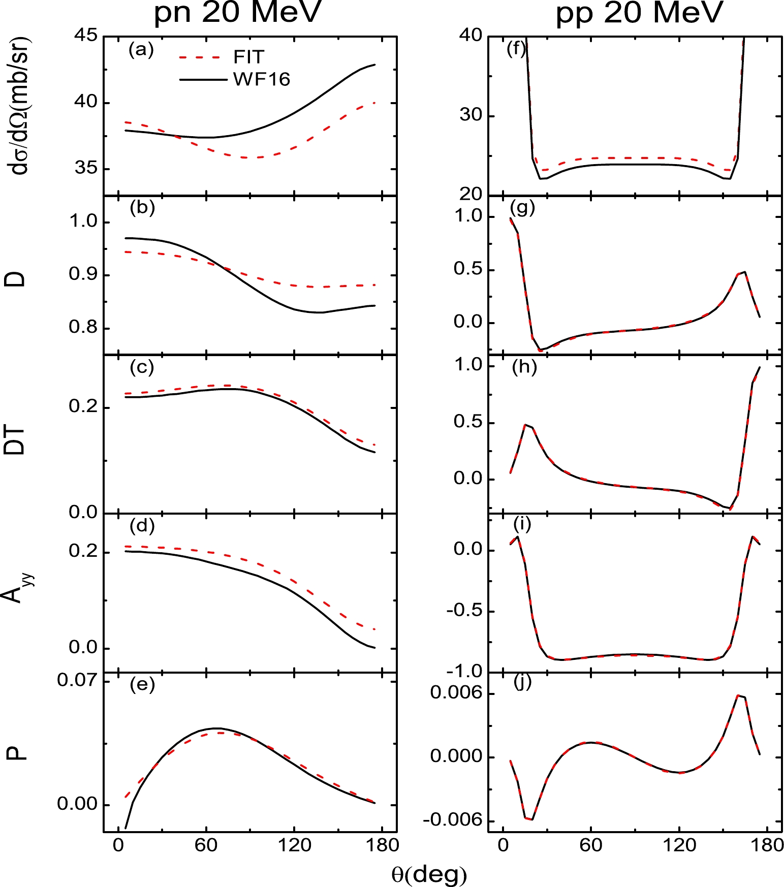

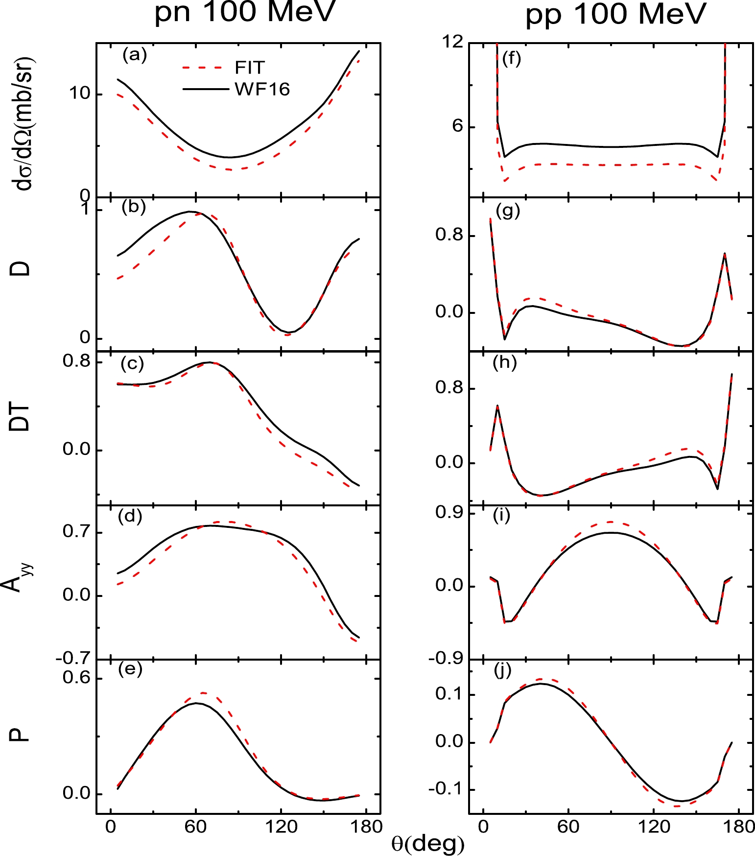
Figure 2

Figure 2.  (color online) np and pp observables as a function of the center-of-mass scattering angle θ for $T_{\rm lab}$ = 20 MeV. The dashed curves are generated from Table 1, and the solid curves are the observables of WF16 [34].

DownLoad: Full-Size Img PowerPoint

Figure 3

Figure 3.  (color online) Same as Fig. 2 but for $T_{\rm lab}$ = 100 MeV.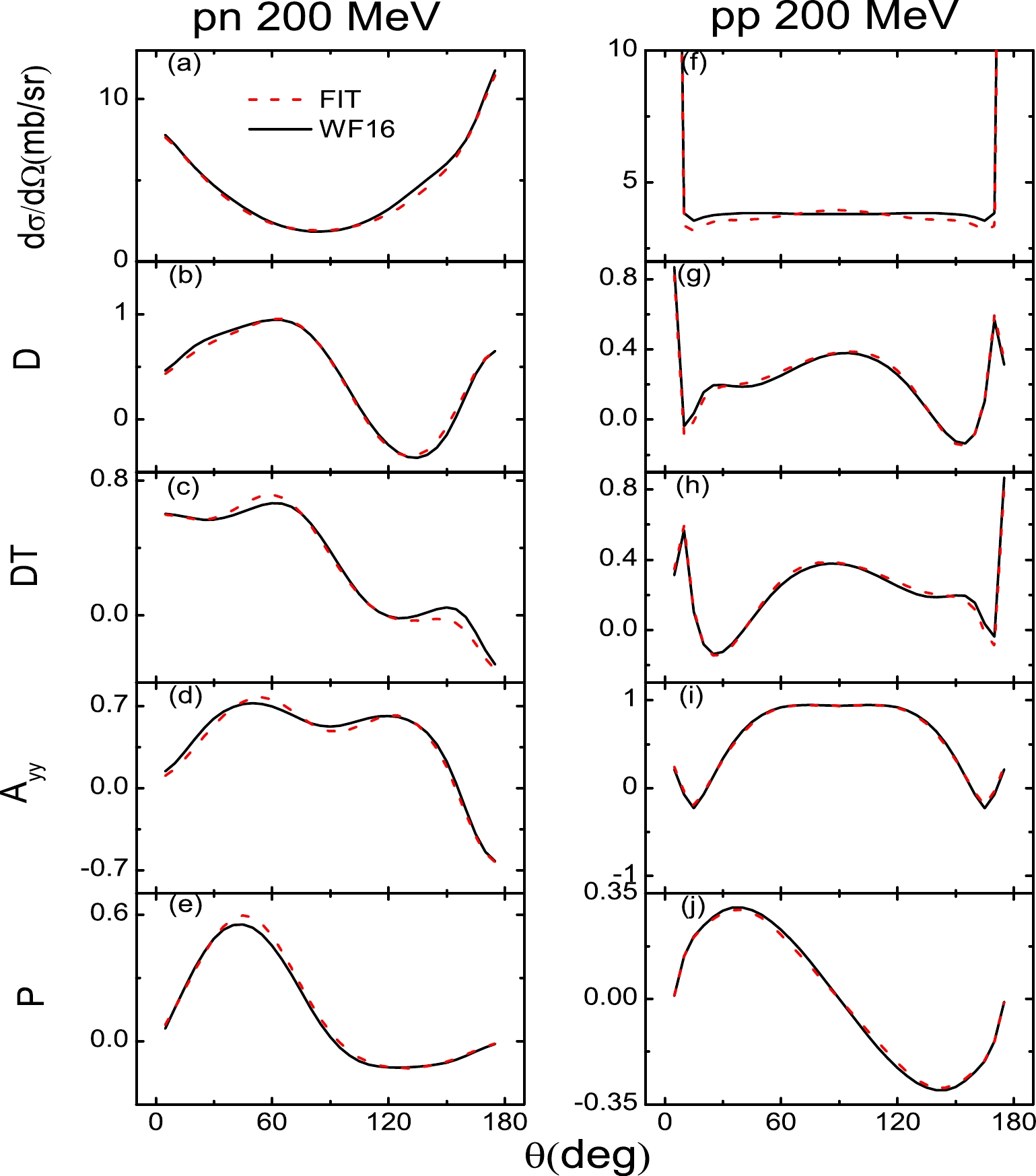

DownLoad: Full-Size Img PowerPoint

Figure 4

Figure 4.  (color online) Same as Fig. 2 but for $T_{\rm lab}$ = 200 MeV.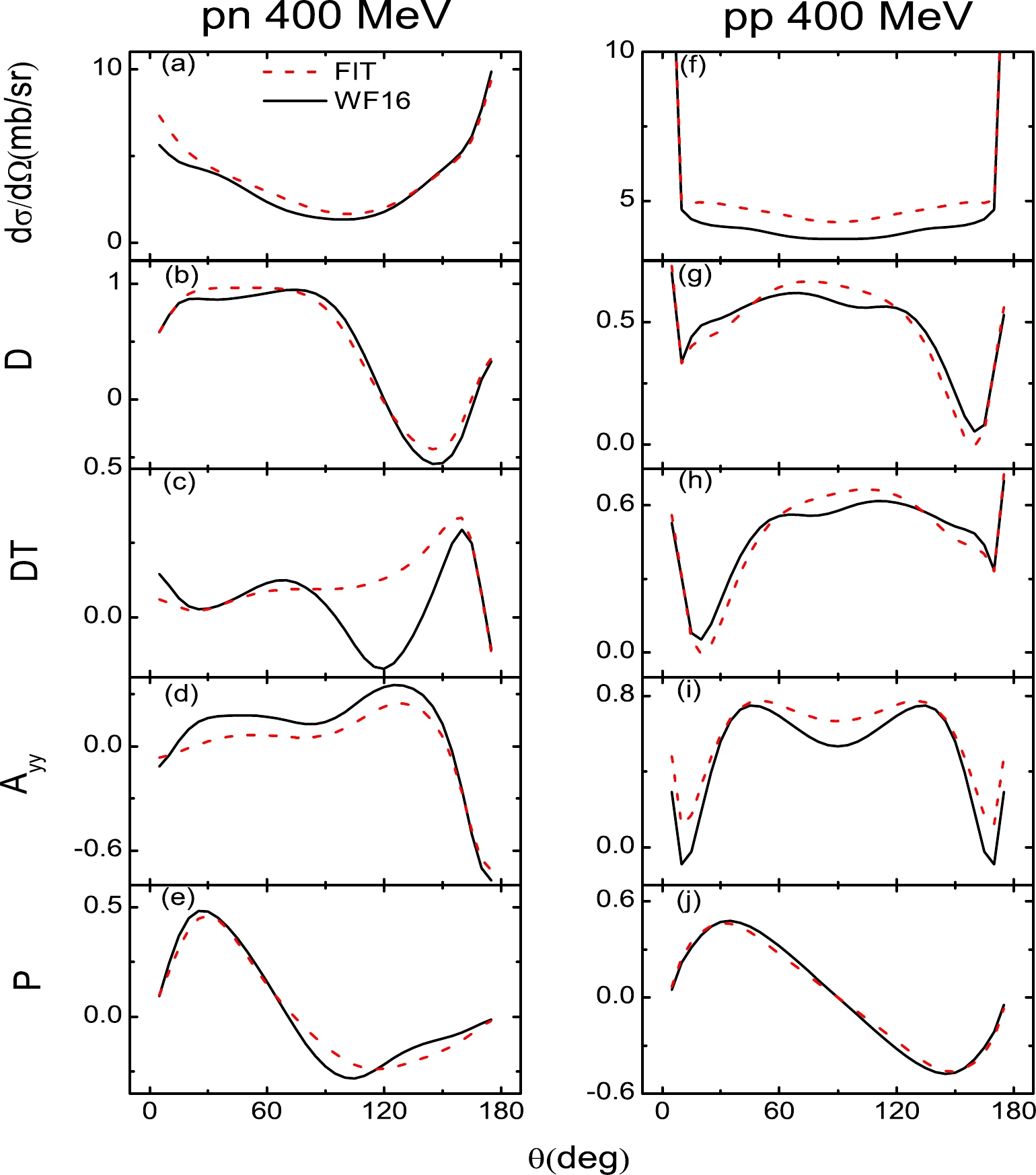

DownLoad: Full-Size Img PowerPoint

Figure 5

Figure 5.  (color online) Same as Fig. 2 but for $T_{\rm lab}$ = 400 MeV.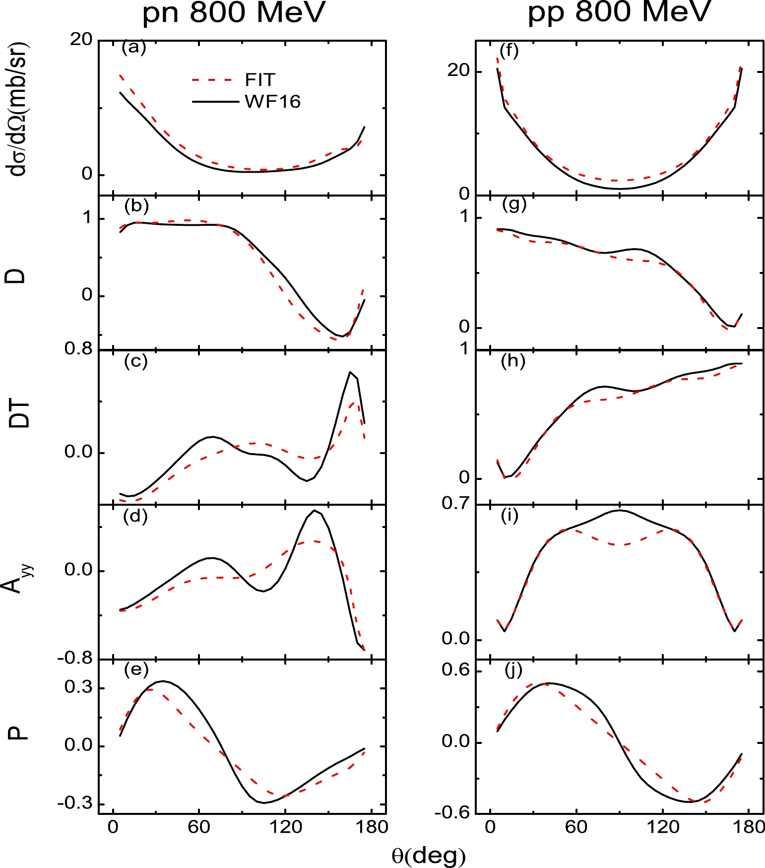

DownLoad: Full-Size Img PowerPoint

Figure 6

Figure 6.  (color online) Same as Fig. 2 but for $T_{\rm lab}$ = 800 MeV.

DownLoad: Full-Size Img PowerPoint

For energies above and below 200 MeV, because the fits cover a wide range of energies, it is expected that the scattering observables are not described as well as those at 200 MeV. As shown in Figs. 2 and 3, for energies far from 200 MeV ($T_{\rm lab}=$ 20 MeV), the unpolarized differential cross section ($\rm\frac{d\sigma}{d\Omega}$) and depolarization tensor for the polarized beam (D) of pn are not perfectly described. However, because the Coulomb corrections of all the pp scattering observables are very significant at energies below 200 MeV, the pp scattering observables are well described. For incident energies above 200 MeV, the results are similar to those of previous studies [11, 12]. As shown in Figs. 5 and 6, the polarization transfer from beam to recoil particle (DT) and polarization correlation for initially unpolarized particles ($A_{yy}$) of pn are not perfectly described. When the Coulomb corrections are included, the pp scattering observables are better described than those of pn. For energies above and below 200 MeV, although some fits are not perfectly described, they are not far from the experiment observables. In conclusion, the RLF model of the NN interaction has been constructed over the laboratory energy range of 20 to 800 MeV.

B Proton-nucleus scattering results and discussions

• I. INTRODUCTION
• II. FORMALISM
• III. RESULTS AND DISCUSSIONS
•      A Fitting procedures and results
•      B Proton-nucleus scattering results and discussions
• IV. SUMMARY
• ACKNOWLEDGMENT

To examine the validity of the above fit, we investigate the p+$^{208}$Pb elastic scattering for a wide energy range ($T_{\rm lab}=$30, 65, 200, 295, 500, and 800 MeV). The differential cross sections ${\rm d}\Omega/{\rm d}\sigma$, analyzing powers $A_y$, and spinrotation functions Q have been investigated with RLF [6, 7]. However, the RLF model has not been used to describe ${\rm d}\Omega/{\rm d}\sigma$, $A_y$, and Q for energies above 400 MeV. Moreover, because the parameters of this work are fitted for a wide energy range, the physical quantities may differ somewhat from those in previous studies. For our calculations, we have taken pseudovector coupling for the pion of RLF. Additionally, because the tensor potential is small, it has been neglected in the calculations.

The PB corrections have been proved to be significant in RLF at low energy [6, 7]. However, the PB correction factors are still model-dependent. The initial PB parameters are obtained via a relativistic Dirac-Brueckner approach [6]. However, the initial PB parameters cannot well describe the ${\rm d}\Omega/{\rm d}\sigma$, $A_y$, and Q in the energy-dependent RLF model [7]. Therefore, the PB factors of the energy-dependent RLF model are obtained by acquiring the best fits of ${\rm d}\Omega/{\rm d}\sigma$, $A_y$, and Q. Because the fits of this work cover a wide range of energies, the PB factors of the previous energy-dependent RLF model may not be able to describe the p+$^{208}$Pb elastic scattering. In order to obtain the PB factors and evaluate our fits, we first compare the optical potentials of this work with the Dirac global optical potentials (GOPs) [1] and the optical potentials of Ref. [7] at 65 MeV. As shown in upper panel of Fig. 7, without considering the PB corrections, the real (Re) values of the optical potentials of this work are similar to those of the previous energy-dependent RLF model, and the imaginary (Im) values of the optical potentials of this work are slightly higher than those of the previous energy-dependent RLF model. These results indicate that the fits of this work are reasonable. The Im values of the optical potentials of both this work and the previous energy-dependent RLF model are higher than those of the GOPs; however, the Re values of the optical potentials of both this work and the previous energy-dependent RLF model are lower than those of the GOPs. The higher Im and lower Re optical potentials imply that the signs of the PB factors of the Im and Re optical potentials in this work should be opposite. At low energy, the extrapolation of Dirac-Brueckner PB factors are too small to properly change the optical potentials. The Im values with PB factors of the phenomenological approach [7] can change the Im values of the optical potentials properly; however, the Re values with PB factors of the phenomenological approach are too low and positive. As shown in the lower panel of Fig. 7, the optical potentials are obtained with the fit of this work and various PB factors. With the extrapolation of Dirac-Brueckner PB factors, the optical potentials do not change much compared with those without the PB corrections. With the PB factors of the phenomenological approach [7], the Im values of the optical potentials are consistent with those of the GOPs, and the Re values of optical potentials are lower than those of GOPs. Therefore, with phenomenological approach, we re-fit the optical potentials by adjusting the PB factors. The PB factors of this work are presented in Table 2. The PB factors of previous studies are also listed, for comparison. The optical potentials with the PB factors of this work are close to the GOPs. When the optical potentials become reasonable, the energy-dependent RLF can well describe the p+$^{208}$Pb scattering.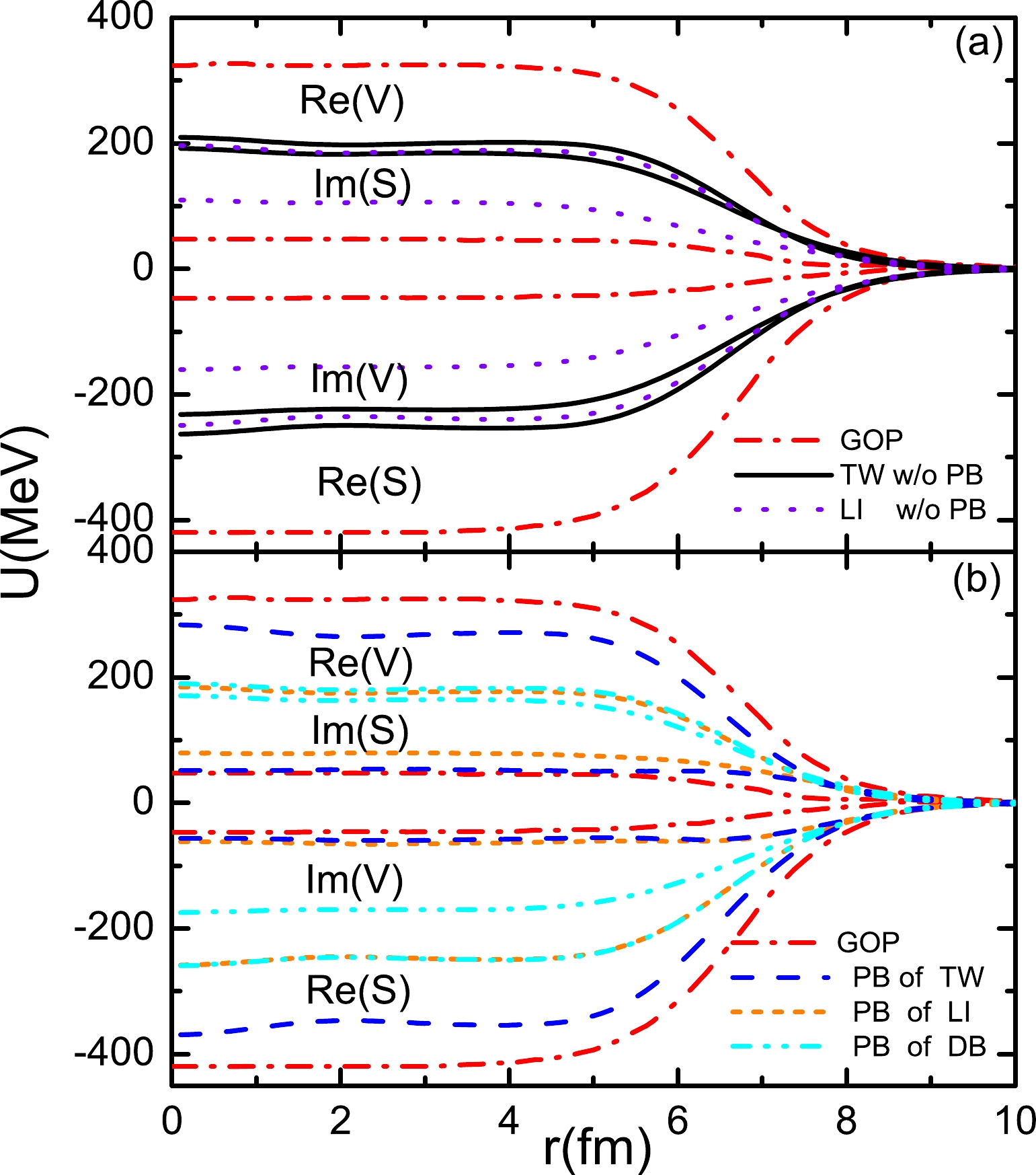

Figure 7

Figure 7.  (color online) The real (Re) and imaginary (Im) parts of the scalar S and vector V optical potentials for p$+^{208}\rm{Pb}$ at 65 MeV. The black solid curves of the upper panel are obtained via the fit of this work (TW) without the Pauli blocking (PB) corrections. The violet dot curves of the upper panel were obtained in Li's work (LI) without PB corrections [7]. The blue dashed curves of the lower panel are obtained by considering the PB corrections of this work. The orange short-dash curves of the lower panel are obtained by considering the PB corrections of Li's work. The cyan dash-dot-dot curves of lower panel are obtained by considering the extrapolation of Dirac-Brueckner (DB) PB corrections [6]. The Dirac GOPs (red dash-dot curves) come from Ref. [1].

DownLoad: Full-Size Img PowerPoint

Table 2

Table 2.  Pauli blocking correction factors $a^L$. The phenomenological Pauli blocking factors [7] and the Pauli blocking correction factors of the Dirac-Brueckner approach [6] are shown for comparison.

The Pauli blocking correction factors of this work
Energy/MeV	Real scalar	Imaginary scalar	Real vector	Imaginary vector
30	−1.30	0.95	−0.85	1.05
65	−0.47	0.85	−0.41	0.88
200	−0.05	0.65	−	0.65
295	−	0.65	−	0.50
500	−	−	−0.05	−
650	−	−	−0.1	−
800	−	−	−0.1	−
The phenomenological Pauli blocking factors
Energy/MeV	Real scalar	Imaginary scalar	Real vector	Imaginary vector
65	0.020	0.68	0.14	0.85
100	0.007	0.60	0.11	0.73
135	0.005	0.53	0.09	0.60
170	0.008	0.42	0.07	0.50
200	0.010	0.35	0.605	0.42
The Pauli blocking correction factors of Dirac-Brueckner approach
Energy/MeV	Real scalar	Imaginary scalar	Real vector	Imaginary vector
135	0.00377	0.11236	0.08403	0.24535
200	−0.0078	0.098	0.0605	0.207
300	−0.0256	0.0759	0.0243	0.148
400	−0.0434	0.061	−0.0119	0.089

DownLoad: CSV

Show Table

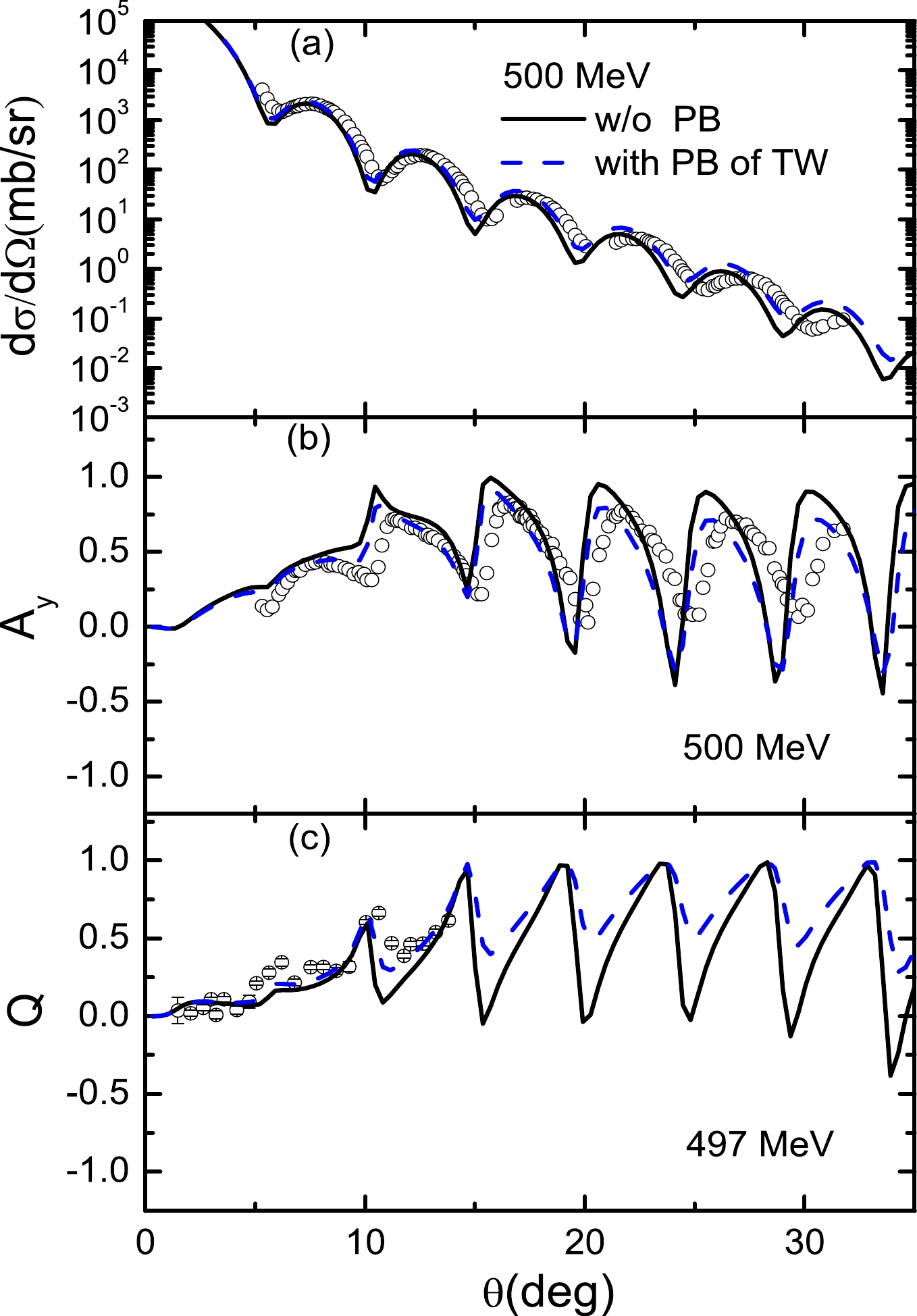
As shown in Fig. 8, the ${\rm d}\Omega/{\rm d}\sigma$ values of $T_{\rm lab}=$65 MeV without PB contributions are lower than the experimental data, and $A_y$ and Q fail to describe the experimental data over the entire angular range. With the PB corrections of this work, the experimental ${\rm d}\Omega/{\rm d}\sigma$, $A_y$, and Q of $T_{\rm lab}=$65 MeV can be well described for the entire angular range. Our predictions of 65 MeV are as good as the previous results obtained by changing $g_\sigma^2$ and $g_\omega^2$[7]. The ${\rm d}\Omega/{\rm d}\sigma$, $A_y$, and Q with the PB corrections of previous studies are also shown, for comparison. In this work, the PB factors of the phenomenological approach [7] and the extrapolation of Dirac-Brueckner fail to describe the ${\rm d}\Omega/{\rm d}\sigma$, $A_y$, and Q. Generally, different fitting methods need different PB corrections to describe elastic scattering. It should be noted that the PB factors of energies below 200 MeV are far larger than the initial PB parameters generated from the relativistic Dirac-Brueckner approach [6]. In the following, we only consider the PB corrections of this work.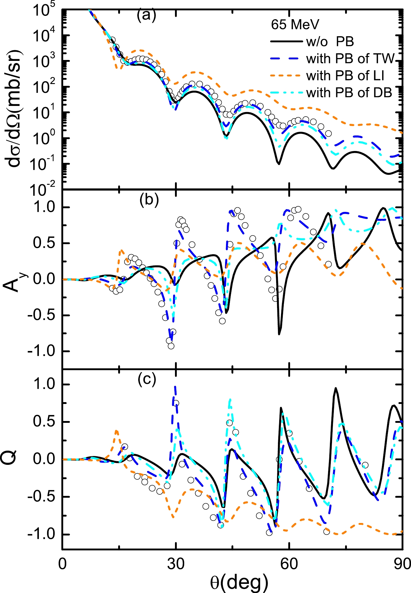

Figure 8

Figure 8.  (color online) Differential cross sections (${\rm d}\Omega/{\rm d}\sigma$), analyzing powers ($A_y$), and spinrotation functions (Q) as a function of the center-of-mass scattering angle for 65 MeV p+$^{208}$Pb scattering. The black solid curves do not include the Pauli blocking (PB) corrections. The blue dashed curves include the PB corrections of this work. The orange short-dash curves of the lower panel are obtained by considering the PB corrections of Li's work (LI) [7]. The cyan dash-dot-dot curves are obtained by considering the extrapolation of PB corrections of Dirac-Brueckner (DB) [6]. The open circles indicate the experimental data taken from Ref. [35].

DownLoad: Full-Size Img PowerPoint

For energies far below 200 MeV, as shown in Fig. 9, the ${\rm d}\Omega/{\rm d}\sigma$ and $A_y$ of $T_{\rm lab}=$30 MeV without PB contributions lack the property of fluctuating with respect to the angle in the p+$^{208}$Pb elastic scattering and cannot describe the experimental data well. When the PB corrections are taken into account, the property of fluctuating with respect to the angle is generated, and the ${\rm d}\Omega/{\rm d}\sigma$ and $A_y$ of 30 MeV can be consistent with the experimental data. For scattering angles smaller than 120 degrees, our result of 30 MeV shows some improvement over the previous results based on changing the real $\sigma N$ and $\omega N$ coupling constants ($g_\sigma^2$ and $g_\omega^2$) [7]. Because the spin observable Q of 30 MeV lacks experimental data, there may be uncertainties in the predictions of 30 MeV.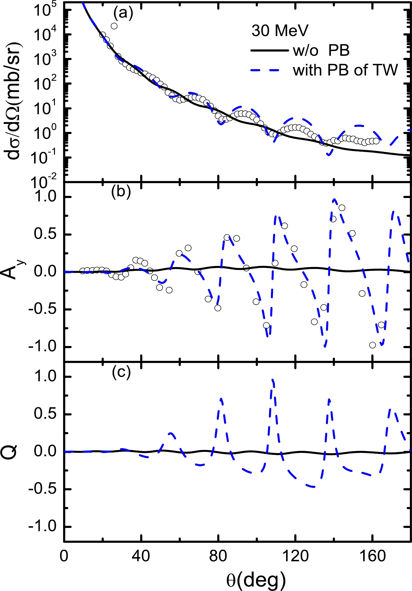

Figure 9

Figure 9.  (color online) Differential cross sections (${\rm d}\Omega/{\rm d}\sigma$), analyzing powers ($A_y$), and spinrotation functions (Q) as a function of the center-of-mass scattering angle for 30 MeV p+$^{208}$Pb scattering. The solid curves do not consider the Pauli blocking (PB) corrections, and the dashed curves consider the PB corrections of this work. The open circles indicate the experimental data taken from Refs. [36, 37].

DownLoad: Full-Size Img PowerPoint

When $T_{\rm lab}=$200 MeV, as shown in Figs. 4 and 10, even though the np and pp scattering observables are the best fit, the experimental ${\rm d}\Omega/{\rm d}\sigma$, $A_y$, and Q without PB contributions cannot fit the experimental data well. In particular, the spin observable Q is poorly fitted for the entire angular range. When the PB corrections are included, the experimental ${\rm d}\Omega/{\rm d}\sigma$, $A_y$, and Q are fitted well for scattering angles smaller than 40 degrees. The result of $T_{\rm lab}=$200 MeV is similar to that of Ref. [7].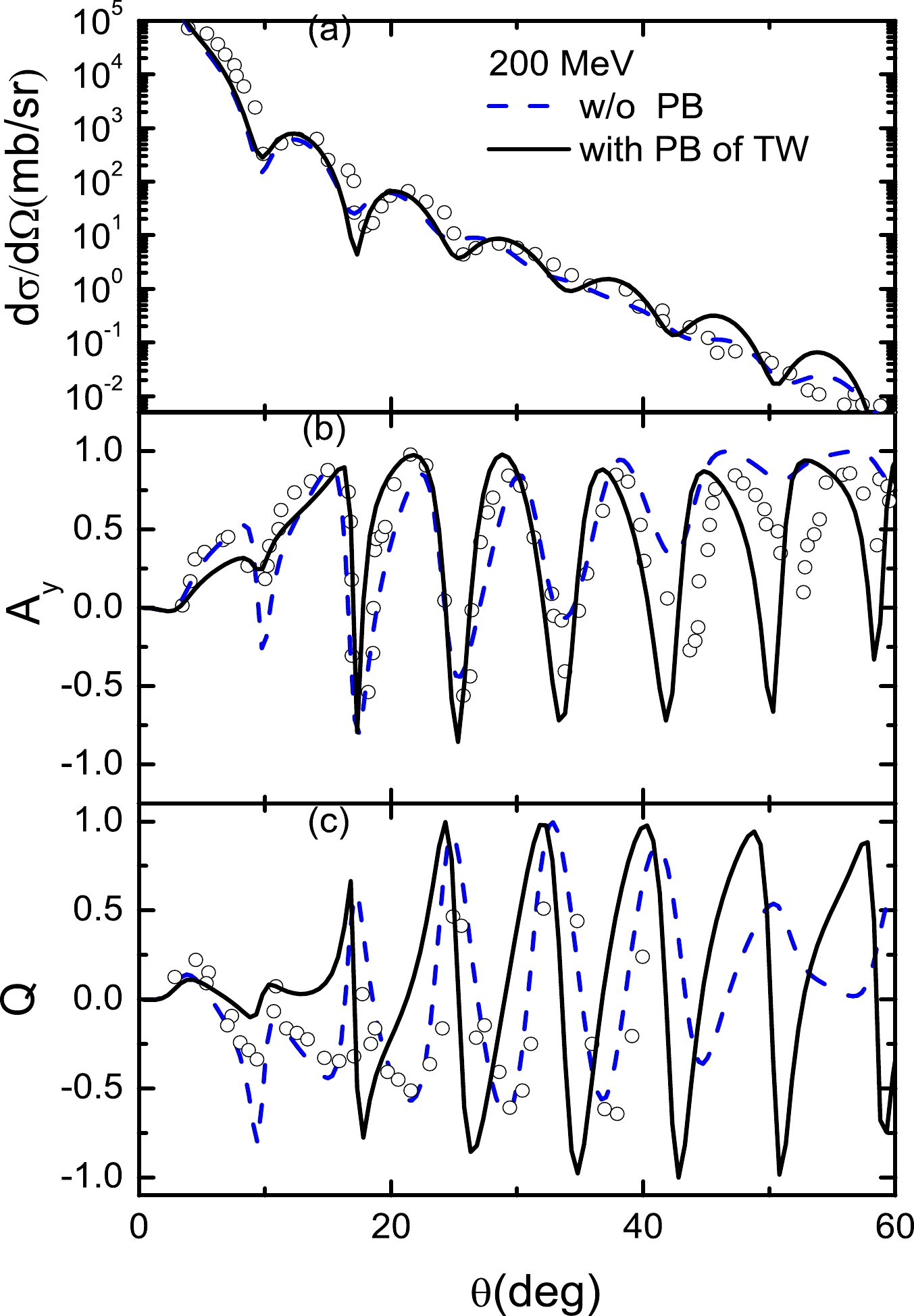

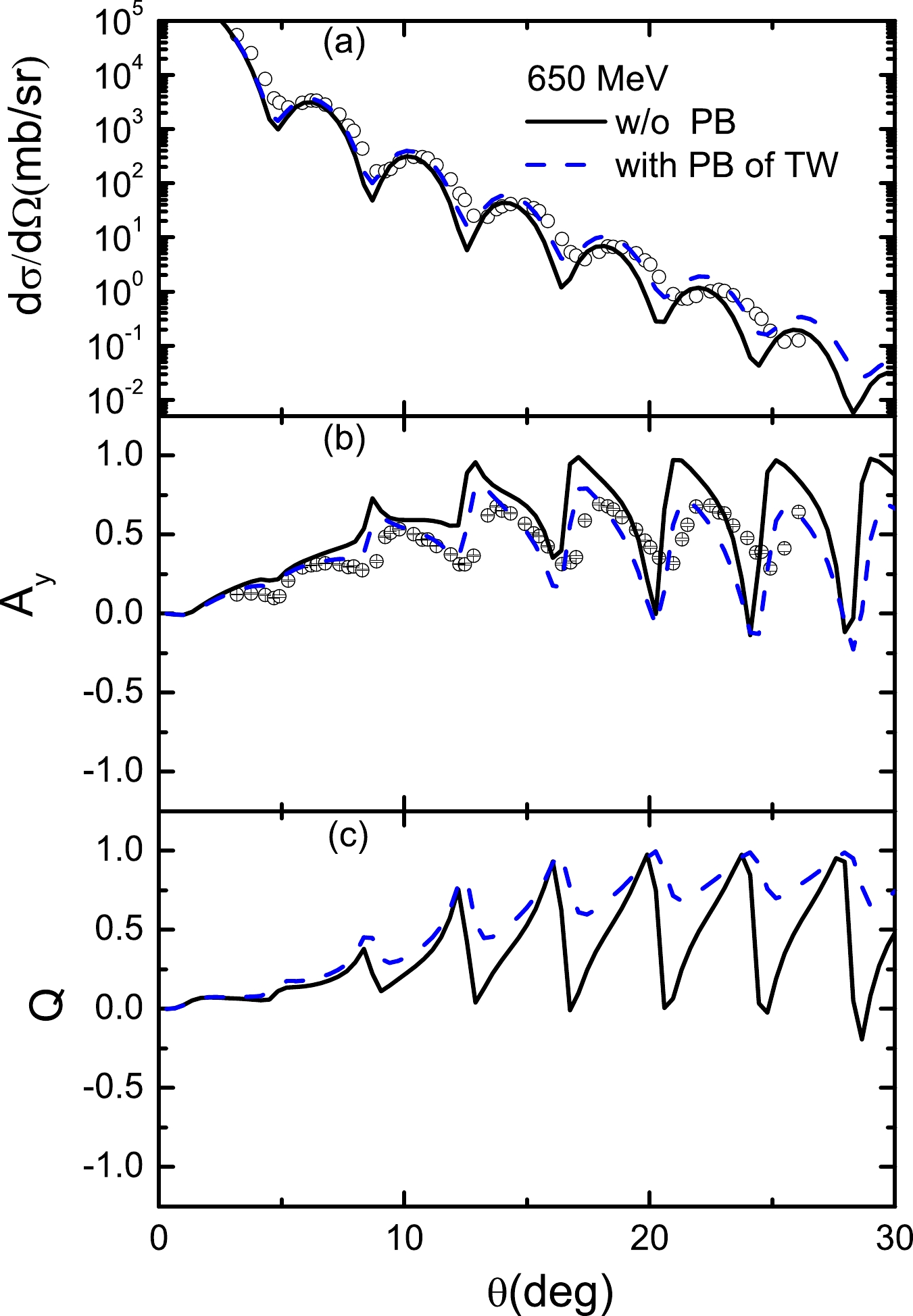
Figure 10

Figure 10.  (color online) Same as Fig. 9 but for 200 MeV p+$^{208}$Pb scattering. The open circles indicate the experimental data taken from Refs. [38–40].

DownLoad: Full-Size Img PowerPoint

For energies above 200 MeV, the situation of PB corrections is complex. When the energy equals 295 MeV, as shown in Fig. 11, the ${\rm d}\Omega/{\rm d}\sigma$ and $A_y$ without PB contributions are not well fitted. When a large imaginary factor of PB contributions is used for $T_{\rm lab}=$295 MeV, the ${\rm d}\Omega/{\rm d}\sigma$ and $A_y$ are only slightly corrected for scattering angles smaller than 30 degrees. As the energy increases, the factors of PB contributions become small; however, the effect of PB corrections cannot be neglected. For instance, as shown in Figs. 12–14, when $T_{\rm lab}=$500, 650, and 800 MeV, the ${\rm d}\Omega/{\rm d}\sigma$, $A_y$, and Q without PB contributions are not described well. When a small factor of the real vector of PB contributions is included, the ${\rm d}\Omega/{\rm d}\sigma$, $A_y$, and Q are fitted better than those in the case without PB contributions.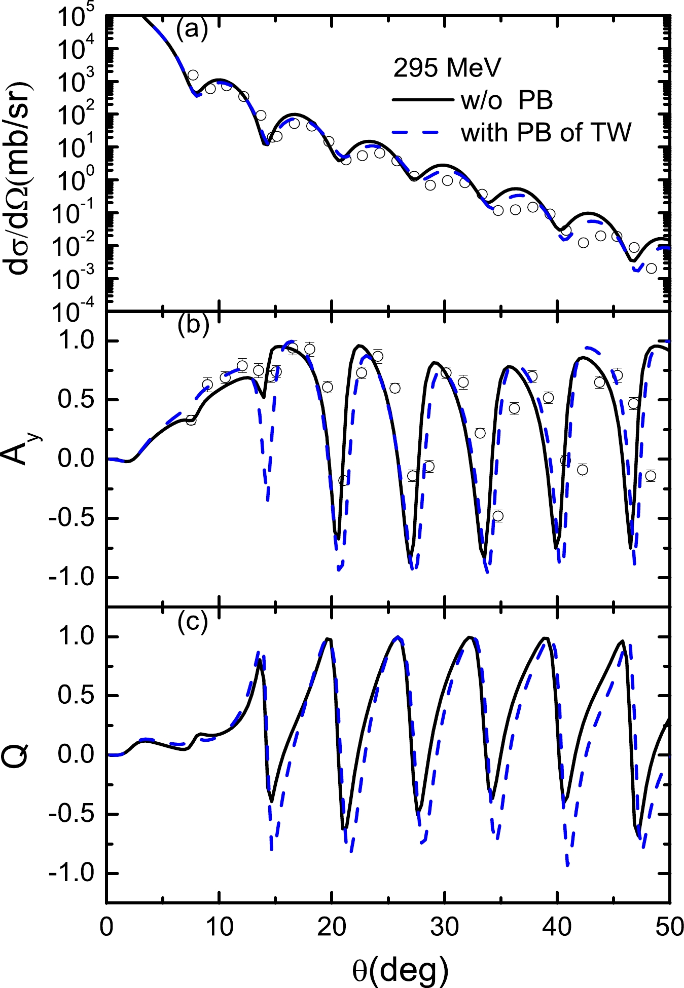

Figure 11

Figure 11.  (color online) Same as Fig. 9 but for 295 MeV p+$^{208}$Pb scattering. The open circles indicate the experimental data taken from Ref. [41].

DownLoad: Full-Size Img PowerPoint

Figure 12

Figure 12.  (color online) Same as Fig. 9 but for 497 and 500 MeV p+$^{208}$Pb scattering. The experimental differential cross sections and analyzing powers of 500 MeV are taken from Ref. [42], and the experimental spinrotation functions of 497 MeV are taken from Ref. [43].

DownLoad: Full-Size Img PowerPoint

Figure 13

Figure 13.  (color online) Same as Fig. 9 but for 650 MeV p+$^{208}$Pb scattering. The open circles indicate the experimental data taken from Ref. [44].

DownLoad: Full-Size Img PowerPoint

Figure 14

Figure 14.  (color online) Same as Fig. 9 but for 800 MeV p+$^{208}$Pb scattering. The open circles indicate the experimental data taken from Refs. [45, 46].

DownLoad: Full-Size Img PowerPoint

IV. SUMMARY

• I. INTRODUCTION
• II. FORMALISM
• III. RESULTS AND DISCUSSIONS
•      A Fitting procedures and results
•      B Proton-nucleus scattering results and discussions
• IV. SUMMARY
• ACKNOWLEDGMENT

The energy-dependent RLF model has been used to fit empirical amplitudes for various energy domains: 50–200, 200–500, and 500–800 MeV. In this work, we try to relate these energy domains within a unified fit. In contrast to previous studies, we fit the scattering observables of pp and pn of WF16 instead of the non-relativistic amplitudes of pp and pn. Because an energy of 200 MeV is chosen as the energy boundary between low and high energy, we first fit the scattering observables of pp and pn of 200 MeV alone. When the scattering observables of pp and pn of 200 MeV are well fitted, the scattering observables of pp and pn of other energies are fitted by using the energy-dependent RLF model. Even though the scattering observables of other energies are not described as well as those of 200 MeV, their trends are consistent with the experimental value, and their values are not far from the experimental values. In conclusion, we constructed the RLF model of the NN interaction over the laboratory energy range of 20 to 800 MeV.

To examine the validity of our fit, we use the energy-dependent RLF model in the range of 20 to 800 MeV to investigate p+$^{208}$ Pb elastic scattering for $T_{\rm lab}=$30, 65, 200, 295, 500, and 800 MeV. The differential cross sections ${\rm d}\Omega/{\rm d}\sigma$, analyzing powers $A_y$, and spin rotation functions Q of p+$^{208}$ Pb elastic scattering without PB corrections are not well fitted at all the energies considered. Although the scattering observables of pp and pn of 200 MeV best fit the experiment values, the RLF model of 200 MeV without PB corrections fails to describe the experimental ${\rm d}\Omega/{\rm d}\sigma$, $A_y$, and Q. For a better description, the PB corrections must be taken into account. We vary the PB factors to obtain the best fits of ${\rm d}\Omega/{\rm d}\sigma$, $A_y$, and Q. In our calculations, the PB factors are larger than those obtained via a relativistic Dirac-Brueckner approach at energies below 295 MeV but similar to those of phenomenological PB effects [7]. For $T_{\rm lab}\geq$500 MeV, the RLF model with a small factor of the real vector of PB contributions can better describe the ${\rm d}\Omega/{\rm d}\sigma$, $A_y$, and Q than those without PB corrections. Our results clearly indicate the importance of PB corrections in the RLF model.

ACKNOWLEDGMENT

• I. INTRODUCTION
• II. FORMALISM
• III. RESULTS AND DISCUSSIONS
•      A Fitting procedures and results
•      B Proton-nucleus scattering results and discussions
• IV. SUMMARY
• ACKNOWLEDGMENT

We thank Ying Kuang and Profs. Zhi-Pan Li and Wei-Zhou Jiang for helpful discussions.

References