


 Abstract
 HTML
HTML Reference
 Related
 PDF
PDF


-
Certain unsolved problems, such as flatness and the horizon, still exist in standard cosmology. Notably, identifying solutions to these problems may be possible if one considers the existence of a phase of inflation in the early universe. Over the years, numerous models capable of generating such an inflationary phase have been proposed. The basis of these old models [1–4] is that the universe began in a thermal equilibrium state and that there exists a Higgs field, which is the inflaton, owing to spontaneous symmetry breaking with a huge amount of energy density for a properly selected effective potential. With regard to the theories regarding inflation, Linde introduced a new paradigm, viz., the "chaotic inflation" [5, 6]. Single-field inflationary models assume the existence of a sufficiently flat potential for the scalar field, which dominates the energy density of the universe. If more than one scalar field is involved, inflation is possible even when the potential is not flat, as discussed elaborately for hybrid inflation by Linde and Bellido [7, 8] and by the assisted inflationary models of Liddle et al. [9]. Thus, in these cases, no ad hoc assumptions on the shape of the potential are required.
However, different unsolved problems still prevail in the inflationary cosmological scenario. Among these problems, the Achilles heel is mostly a cosmological constant problem owing to a huge gap between the observational value of the vacuum energy density and theoretical predictions [10–12]. The upper bound of the observational data [13, 14] corresponding to the vacuum energy density (
$ \rho_{\Lambda} $ ) obtained by Komatsu et al. is 120 orders smaller than the theoretically predicted values of different models. In the study conducted by Weinberg [10], different approaches were adopted for obtaining solutions to this problem. In particular, Wetterich [15] proposed a model, wherein the energy momentum tensor was adjusted dynamically such that the cosmological constant became time-dependent. A large vacuum energy density is usually necessary in different inflationary models to produce sufficient inflation. It can be predicted that the cosmological constant (Λ) had a large value during early times, which is consistent with the theoretical predictions reported by Paul et al. [16]. A few phenomenological Λ models focus on the importance of the time-dependent variable Λ; these include the models proposed by Ray et al. [17] and Mukhopadhyay et al. [18]. Some definite dynamical models [19, 20] of Λ have been selected for inspecting the nature of dark energy. The variability of the cosmological constant in the form of dark energy has been discussed by Peebles and Ratra [21]. A simple toy model has been proposed by Bhattacharyya et al. [22], and it includes the end of inflation to avoid possible deadlock; moreover, the results agree well with the observational data reported by Dunkley et al. [23], Ade et al. [24, 25], and Akrami et al. [26]. A recent study conducted by Basilakos et al. [27] revealed a dynamical process of decaying vacuum energy density from inflation to the radiation phase, which is followed by the dark matter and vacuum regimes. In connection with inflationary cosmology, certain interesting studies related to dark energy are available in the literature [28–30].In the context of general relativity, conformal re-scalings and conformal techniques have been adopted extensively. Different models of inflation (e.g., Kalara et al. [31]) based on non-minimal gravity can be treated in a similar manner as standard inflationary analyses using conformal transformations. Certain applications of conformal transformations [32] to a general class of single field inflation models of gravity and non-standard kinetic terms with non-minimal coupling have been proposed by Kubotam et al. Over the years, the technique of Weyl or conformal transformation has been adopted [33–36], based on which the cosmological constant is assumed to decrease as time progresses.
In the present study, we mainly focus on the duration of the inflationary phase and use the progressive technique proposed by Darabi [37] and Bisabr [38, 39]. This progressive technique is important in terms of the quintessence theory as it predicts that dark energy is a new force that will fade away just as it emerged. In our analysis, we make two assumptions for our model. The first assumption relates to the existence of a large effective cosmological constant in the early universe. In the present study, we model the cosmological constant term using an inflaton, which is a minimally coupled scalar field, and the corresponding potential has contributions from different fields characterizing particle physics. The second assumption deals with the fact that there exists a conformal background metric that couples with the large energy density, i.e., it is related to the gravitational coupling of the cosmological term. In the presence of gravitational coupling, the conformal factor turns into a damping factor in the cosmological term that is responsible for the reduction in the latter during inflation. As the potential of the scalar field reduces during the inflationary phase, the universe undergoes power law inflation (PLI) and not de Sitter inflation. In the present study, the PLI justifies the small value of the cosmological constant (i.e., the vacuum energy) at later times, and it solves the horizon and flatness problems.
The inflationary scenario has been mostly successful in describing the present universe. This is why one of the major objectives of the cosmic microwave background (CMB) study is the verification of inflation models. However, numerous unanswered questions relating to this scenario, particularly at later times, still prevail. These questions are particularly concerned with how the foregoing scenario can lead to the current accelerating phase of the universe, as well as with the events occurring before the initiation of the inflationary mechanism. In addition, the exact nature of the inflaton field is yet to be determined. Numerous speculations on the initiation of the inflationary mechanism have been made to date. Among these, one of the speculations assumes that the universe at extremely high energy densities and small length scales must be dominated by quantum mechanical effects, and there may have been a quantum mechanical tunnelling process leading to the initiation of inflation. However, if the universe was indeed dominated by radiation before inflation began, it must have been geodesically incomplete in the past, encountering a curvature singularity in the finite past. Another possibility is that a non-singular bounce experienced by a contracting universe could have given rise to inflation. The final alternative is an inflationary universe emerging from a universe existing in an eternally quasi-static state.
The outline of the manuscript is as follows: In Sec. II, the basic features of the slow-roll parameters in the conventional PLI with an exponential potential are summarized. In Sec. III, the progressive technique based on conformal transformation for a monomial potential is discussed. We present the field equations and evaluate their exact solutions. We observe that the solutions exhibit a PLI for a power-law potential of the scalar inflaton. Sec. IV presents a comparison of the results obtained using this model with recent observational data. In Sec. V, we provide certain concluding remarks.
-
In a single-field inflationary model, the Lagrangian density can be written as
$ {\mathcal{L}}(g_{\alpha\beta}, \psi)=\frac{1}{2}g^{\alpha\beta}\nabla_{\alpha}\psi\nabla_{\beta}\psi+V(\psi), $

(1) where ψ is the inflaton field, and the potential function is represented by
$ V(\psi) $ .The full action with the unit
$ \hbar=c=1 $ is given by$ S=\frac{1}{16\pi G} \int {\rm d}^{4}x \sqrt{-g} {\mathcal{R}} - \int {\rm d}^{4}x \sqrt{-g}\mathcal{L} , $

(2) where the first term represents the Einstein–Hilbert action.
If we consider the universe to be isotropic and homogeneous, the evolution of the inflaton field
$ \psi(t) $ and the scale factor$ a(t) $ can be expressed by the Friedmann equation:$ 3H^2=k\left[\frac{1}{2}\dot{\psi}^2+V(\psi)\right], $

(3) $ \begin{array}{*{20}{l}} \ddot{\psi}+3H\dot{\psi}=-V'(\psi), \end{array} $

(4) where the Hubble parameter
$ H=\dfrac{\dot{a}}{a} $ , and$ k=8\pi G $ . The dot represents differentiation with respect to t, whereas prime indicates differentiation with respect to ψ. When the slow-roll parameters are small, we note a period of accelerated expansion, i.e., inflation, and the corresponding slow-roll parameters can be written as [40]$ \epsilon(\psi)=\frac{m_p^2}{2}\left[\frac{V'(\psi)}{V(\psi)}\right]^2, $

(5) $ \eta(\psi)=m_p^2\left[\frac{V''(\psi)}{V(\psi)}\right]. $

(6) Here,
$ {m_p}^2=\dfrac{1}{G} $ , and$ m_p $ denotes the Planck mass. As the slow-roll parameters are small, the time-derivatives of ψ in Eqs. (3) and (4) can be justifiably ignored, and the potential term is much greater than the kinetic term, i.e.,$ \dfrac{1}{2}\dot{\psi}^2 \ll V(\psi) $ . Thus, Eq. (3) becomes$ 3H^2\approx k V(\psi) $ . Therefore, when$ \psi \approx $ constant, the energy density corresponding to the scalar field has a constant value, which results in a de sitter solution.In addition to exponential acceleration, non-exponential accelerated expansion can also perform work [41–43]. One may consider, for instance, a power law expansion, and the corresponding scale factor is given by
$ a(t)\sim t^q $ , where the power law index q is greater than unity ($ q>1 $ ). In the conventional PLI, the canonical scalar field has an exponential potential of the form$V(\psi)=V_0{\rm e}^{-\sqrt{\frac{2}{q}}(\frac{\psi}{M_p})}$ , with$ V_0 $ as a constant [44–48]. With the exponential potential, the slow-roll parameters from Eqs. (5) and (6) can be written as$ \epsilon=\frac{1}{q}, $

(7) $ \eta=\frac{2}{q}. $

(8) Within the slow-roll paradigm,
$ \epsilon, \eta\; \ll 1 $ , and hence,$ q\gg 1 $ . For the de Sitter inflationary paradigm, the exponential expansion terminates when the slow-roll approximation is no longer applicable. In the PLI, q is a constant parameter, and hence, the termination of inflation is not clear. Thus, an exit mechanism should be incorporated into the entire inflationary scenario such that with a progress in the expansion, the inflationary phase matches the standard hot Big Bang model, i.e., the radiation or the matter dominated region.Any given inflationary model is usually characterized by the scalar spectral index,
$ n_s $ , and the tensor-to-scalar ratio, r [49, 50]. These two parameters are related to the slow-roll parameters ($ \epsilon, \eta $ ) as$ \begin{array}{*{20}{l}} n_s-1 = 2\eta-6\epsilon, \end{array} $

(9) $ \begin{array}{*{20}{l}} r = 16\epsilon. \end{array} $

(10) For the PLI, we have
$ n_s-1 = -\frac{2}{q}, $

(11) $ r = \frac{16}{q}. $

(12) The Planck data [24], combined with the Wilkinson microwave anisotropy probe (WMAP) result [23], require that the value of the scalar spectral index (
$ n_s $ ) be in the range of$ n_s\in [0.945, 0.98] $ and the tensor-to-scalar ratio be$ r<0.11 $ (in the model Planck TT+lowP+BAO). The constraint originating from a combination of the Planck [26], BICEP2, and Keck Array data [25, 26] is$ r<0.07 $ . The observational limits on$ n_s $ are equivalent to the limits of the power law index,$ 38\leq q \leq 101 $ , which correspond to$ 0.16 < r < 0.43 $ . This range of r lies beyond the above-mentioned ranges. In Fig. 2, the outermost and middle contours represent the Planck + WP data, and the innermost contour corresponds to the Planck + BICEP2 + Keck Array data. The solid line representing the PLI lies completely outside the outer contour.Thus, the conventional PLI has two drawbacks. The first problem is the graceful exit problem, and the second is the mismatch between observations and theoretical predictions. Hence, one must clarify the Lagrangian density corresponding to the inflaton so that
$ n_s $ and r become consistent with the observational data [43, 51]. -
Conformal transformation is typically used as a mathematical tool to map the equations of motion between physical systems and mathematically equivalent sets of equations, rendering them easier to solve and computationally more convenient to study. In this model, we make two assumptions regarding the gravitational coupling of matter systems. First, different types of matter couple with a particular metric. This implies that all types of fields in different standard models couple in a similar manner to gravity, irrespective of extensive variations in their physical properties. Second, we consider a unique metric describing the background geometry. Thus, gravitational coupling is universal, and the equivalence principle supports this fact with numerous observable results, such as those presented by Damour [52, 53]. This has also been verified empirically several times since the seventeenth century [54, 55]. In this case, the results are extrapolated to the total age of the universe because all the equivalence principle tests have been conducted within a limited time interval (four hundred years since the time of Galileo). However, there exists a possibility that the equivalence principle has been violated at some point during the evolution of the universe. Further, all the equivalence principle tests are restricted to the solar system. It is well known that there exist some screening techniques, based on which the anomalous gravitational coupling of matter can be obscured from experiments, e.g., if a chameleon scalar field interacts with matter [56, 57]), such an interaction cannot be detected empirically. In this case, the local gravity constraints are suppressed in the laboratory as the chameleon field is heavy. Meanwhile, the field can be sufficiently light in the low-density cosmological environment to produce observable effects on a large scale.
In this study, we attempt to consider gravitational coupling to cool off the aforementioned assumptions. We also consider the fact that the two metrics for the matter and gravitational sectors relate to different conformal frames. In this case, we consider a minimally coupled scalar field as depicted by the Lagrangian density (1). As we consider contributions resulting from the various fields of elementary particles, the potential of the inflaton ψ has a large effective mass, which corresponds to a large effective cosmological constant. Further, we consider in the full action that the inflaton part pertains to a different conformal frame [58, 59]. Thus,
$ \bar{g}_{\alpha\beta} ={\rm e}^{-2\xi} g_{\alpha\beta}, $

(13) $ \begin{array}{*{20}{l}} \bar{\psi} = {\rm e}^{\xi} \psi. \end{array} $

(14) From Eq. (13), the inverse metric
$ g^{\alpha\beta} $ and the determinant g = det[$ g_{\alpha\beta} $ ] transform as$ \begin{array}{*{20}{l}} \bar{g}^{\alpha\beta} ={\rm e}^{2\xi} g^{\alpha\beta}, \end{array} $

(15) $ \begin{array}{*{20}{l}} \sqrt{-\bar{g}} = {\rm e}^{-4\xi} \sqrt{-g}. \end{array} $

(16) We consider the conformal transformations as local unit transformations [60–65] with a space-time dependent conversion factor. Usually, ξ depends on the space-time, and it is a smooth, dimensionless function. However, later in the calculation, we will assume that ξ is a function of time only. Hence, the Lagrangian density corresponding to the inflaton can be written as
$ {\mathcal{L}}(\bar{g}_{\alpha\beta}, \bar{\psi})=\frac{1}{2}\bar{g}^{\alpha\beta}\nabla_{\alpha}\bar{\psi}\nabla_{\beta}\bar{\psi}+V(\bar{\psi}). $

(17) Based on the fact that the Lagrangian is invariant under a conformal transformation, the full action from Eq. (2) is given by
$ \begin{eqnarray} S=\frac{1}{2k} \int {\rm d}^{4}x \sqrt{-g} {\mathcal{R}} -\int {\rm d}^{4}x \sqrt{-\bar{g}} {\mathcal{L}}(\bar{g}_{\alpha\beta} \bar{\psi}). \end{eqnarray} $

(18) In terms of
$ g_{\alpha\beta} $ and ψ, the action in Eq. (18) becomes$ \begin{aligned}[b] S =&\frac{1}{2} \int {\rm d}^{4}x \sqrt{-g}\bigg\{\frac{1}{k}{\mathcal{R}}-g^{\alpha\beta} \nabla_{\alpha} \psi \nabla_{\beta}\psi \\& -2\psi g^{\alpha\beta} \nabla_{\alpha} \psi \nabla_{\beta}\xi -\psi^2 g^{\alpha\beta} \nabla_{\alpha} \xi \nabla_{\beta}\xi -V({{\rm e}^{\xi}}\psi){\rm e}^{-4\xi}\bigg\}. \end{aligned} $

(19) The action functional thus obtained depends on two scalar fields, viz., ξ and ψ, which are dynamical in nature with a term belonging to the mixed kinetic type [66, 67]. This type of system has an important application in the formulation of assisted quintessence [68–71], as well as in the amelioration of different dark energy models [67, 72, 73].
We may consider the following:
$ \begin{array}{*{20}{l}} \psi g^{\alpha\beta} \nabla_{\alpha}\psi \nabla_{\beta}\xi = \nabla_{\alpha} (\psi \xi g^{\alpha\beta}\nabla_{\beta}\psi)-\xi g^{\alpha\beta} \nabla_{\alpha} \psi\nabla_{\beta}\psi-\psi \xi \Box\psi. \end{array} $

(20) Using Eq. (20), the action in Eq. (19) can be written as
$ \begin{aligned}[b] S =&\frac{1}{2} \int {\rm d}^{4}x \sqrt{-g} \bigg\{\frac{1}{k}{\mathcal{R}}-(1-2\xi)g^{\alpha\beta} \nabla_{\alpha} \psi \nabla_{\beta}\psi \\& - 2\psi \xi \Box \psi -\psi^2 g^{\alpha\beta} \nabla_{\alpha} \xi \nabla_{\beta}\xi -V({\rm e}^{\xi}\psi){\rm e}^{-4\xi}\bigg\}. \end{aligned} $

(21) It should be noted from Eq. (21) that the scalar field has a dimension of
$ L^{-1} $ or M in a natural unit system. However, the conformal factor is dimensionless. Thus, ξ is a dynamical variable but not a scalar field, and hence, in Eq. (21), we only have one scalar field.When the slow-roll condition is valid, we can write
$ \begin{array}{*{20}{l}} \{(\partial \psi)^2, \Box \psi \} \ll V({\rm e}^{\xi}\psi){\rm e}^{-4\xi}. \end{array} $

(22) Thus, Eq. (21) can be approximated to
$ S=\frac{1}{2} \int {\rm d}^{4}x \sqrt{-g} \left\{\frac{1}{k}{\mathcal{R}} -\psi^2 g^{\alpha\beta}\partial_{\alpha} \xi \partial_{\beta}\xi-V({\rm e}^{\xi}\psi){\rm e}^{-4\xi}\right\}. $

(23) It is well known that during inflation, the potential term is much greater than the kinetic term. Hence, the approximation depicted in Eq. (22) is justified, implying that Eq. (23) is correct. However, we can use Eq. (23) instead of the full action in Eq. (21). It is also interesting to note the existence of an exponential coefficient in the potential term. If ξ increases with time, the coefficient plays the role of a damping factor, and the potential decreases.
-
As an example, we consider a potential of the form [6]
$ V(\bar{\psi})= \nu m_p^4\left(\frac{\bar{\psi}}{m_p}\right)^p,$

(24) where ν and p are constant quantities with
$ \nu\ll 1 $ .The corresponding slow-roll parameters are given by
$ \epsilon=\frac{p^2}{2\gamma^2}\; ,\; \eta=\frac{p(p-1)}{\gamma^2}, $

(25) where
$ \gamma \equiv \psi/m_p $ , and during slow-roll inflation, we can write$ \gamma \gg 1 $ , which will be discussed later in this section.With this, from Eq. (23) and using the monomial potential in Eq. (24), we have
$ \begin{aligned}[b] S=&\frac{1}{2} \int {\rm d}^{4}x \sqrt{-g} \Bigg[\frac{1}{k}{\mathcal{R}} -\psi^2\Big\{g^{\alpha\beta} \partial_{\alpha} \xi \partial_{\beta}\xi\\&+ \nu m_p^{4-p}\psi^{p-2} {\rm d}^{(p-4)\xi}\Big\}\Bigg]. \end{aligned} $

(26) Varying the action with respect to
$ g_{\alpha\beta} $ and ξ produces the required field equations in a spatially flat FRW background, as follows:$ 3 \left(\frac{\dot{a}}{a}\right)^2=\frac{1}{2}k \psi^2\left\{\dot{\xi}^2+\nu m_p^{4-p}\psi^{p-2} {\rm d}^{(p-4)\xi}\right\}. $

(27) $ \ddot{\xi}+3H \dot{\xi}+\frac{1}{2}(p-4)\nu m_p^{4-p}\psi^{p-2} {\rm e}^{(p-4)\xi}=0. $

(28) The corresponding solution can be provided as follows [31]
$ \begin{array}{*{20}{l}} a(t)=a_{0} t^q , \end{array} $

(29) $ \xi(t)=\xi_T - C\ln {\left(\frac{t}{t_T}\right)}, $

(30) where
$\begin{aligned}[b]& q= 4\pi C^2\gamma^2,\quad C=\frac{2}{(p-4)} \; \;\text{and}\; \\& t_T^2=\left[\frac{4(3q-1)}{\nu \gamma^{p-2}(p-4)^2m_p^2 {\rm e}^{(p-4)\xi_T}}\right]. \end{aligned} $

(31) In this case,
$ \xi_T $ is a constant, which is a dimensionless quantity and represents the value of ξ when the inflation terminates. However, following the approach adopted by Kalara et al. [31], one can opt for simplified forms of Eqs. (29)–(31).From Eq. (31), we can assert that during a power law inflationary phase, the universe results in
$ \gamma>\dfrac {|p-4|}{4\sqrt{\pi}} $ . Here, the values of ψ from$ -\infty $ to$ +\infty $ are completely appropriate. If$ \rho_{\psi} $ is the energy density of ψ, and$ \rho_{\psi}< m_p^4 $ , the universe can be described classically. As$ \nu \ll 1 $ , one can constrain the kinetic energy of ψ, viz.,$ (\partial\psi)^2<m_p^4 $ [5, 6].From Eq. (30), it is evident that
${\rm e}^{(p-4)\xi}$ decreases with t. Thus,$\Lambda_{\rm eff}\equiv 4\pi\nu m_p^2\gamma^p {\rm e}^{(p-4)\xi}$ reduces during the inflationary phase such that$\Lambda_{\rm eff}\sim t^{-2}$ . This result matches well with the observational upper limit and with the phenomenological models proposed by Ray et al. [19] and Mukhopadhyay et al. [20]; in these studies, it was concluded that for a flat universe,$ \Lambda\sim t^{-2} $ is true for different models.To discriminate among the different components that may be responsible for the present acceleration of the universe [74, 75], two new geometrical parameters, termed as the statefinder parameters, which depend on the nature of the space-time metric, were introduced by Sahni et al. [76]. These parameters are usually denoted by r and s, but here, we will denote them by
$ r' $ and$ s' $ . The parameters are defined, along with the deceleration parameter$q_{\rm dec}$ , as$ q_{\rm dec}=-1-\frac{\dot{H}}{H^2}, $

(32) and
$ r'=1+\frac{3\dot{H}}{H^2}+\frac{\ddot{H}}{H^3},\; s'=\frac{r'-1}{3\left(q_{\rm dec}-\frac{1}{2}\right)}. $

(33) Using the form of a obtained in Eq. (31), the deceleration and statefinder parameters can be determined to be
$ q_{\rm dec}=-\left(\frac{q+1}{q}\right),\; r'=1+\frac{2-3q}{q^2},\; s= \frac{2}{q}\left(\frac{3q-2}{3q+2}\right). $

(34) We can observe from the above result that despite using a scalar field inflaton to generate the inflationary mechanism, both the statefinder parameters are determined to be constants, which is also the case for the Λ-term. Thus, our description of the inflationary mechanism in terms of
$\Lambda_{\rm eff}$ is further established.Another important point regarding the inflationary model is the exit mechanism, i.e., the mechanism of inflation termination. The exit mechanism has been previously identified as a serious problem in the PLI. In the present study, graceful exit occurs owing to the decay of vacuum density. The inflaton ψ is freezed during the slow-roll paradigm, and the corresponding energy density of ψ is given by
$\rho_{\psi}\equiv\dfrac{1}{2}\dot{\psi}^2+V{\rm e}^{-4\xi}\approx V{\rm e}^{-4\xi}$ . Unlike exponential inflation, the energy density$ \rho_{\psi} $ in the present case does not remain constant but decays during inflation. With the evolution of time,$V{\rm e}^{-4\xi}$ reduces. Thus, at a particular stage, there will exist an instant in time when the kinetic term cannot be neglected in$ \rho_{\psi} $ . At this point in time, the kinetic and potential terms will have the same order of magnitude, i.e., the slow-roll approximation will no longer be valid at this stage, and inflation will terminate.After the inflationary paradigm, the reheating stage initiates, and during this stage, the inflaton begins oscillating near the minimum of its effective potential; consequently, elementary particles are produced. These particles interact with each other and ultimately create a state of thermal equilibrium for the universe at some temperature. During reheating, the inflaton energy is converted into matter and radiation, after which the universe re-enters the hot Big Bang model phase, followed by the dark matter and vacuum phases. In this model, we deal with two dynamical scalar fields; however, the reheating process is actually controlled by the inflaton ψ. At the end of the inflation, the conformal factor tends to have a constant configuration, and the kinetic energy part of the inflaton, which was unimportant during inflation, now becomes important. Indeed, the parts of ψ and ξ change during the phase of reheating, and the model is again reduced to a single-field type. In the present case, the reheating process proceeds in a similar manner as that in the standard Big Bang model.
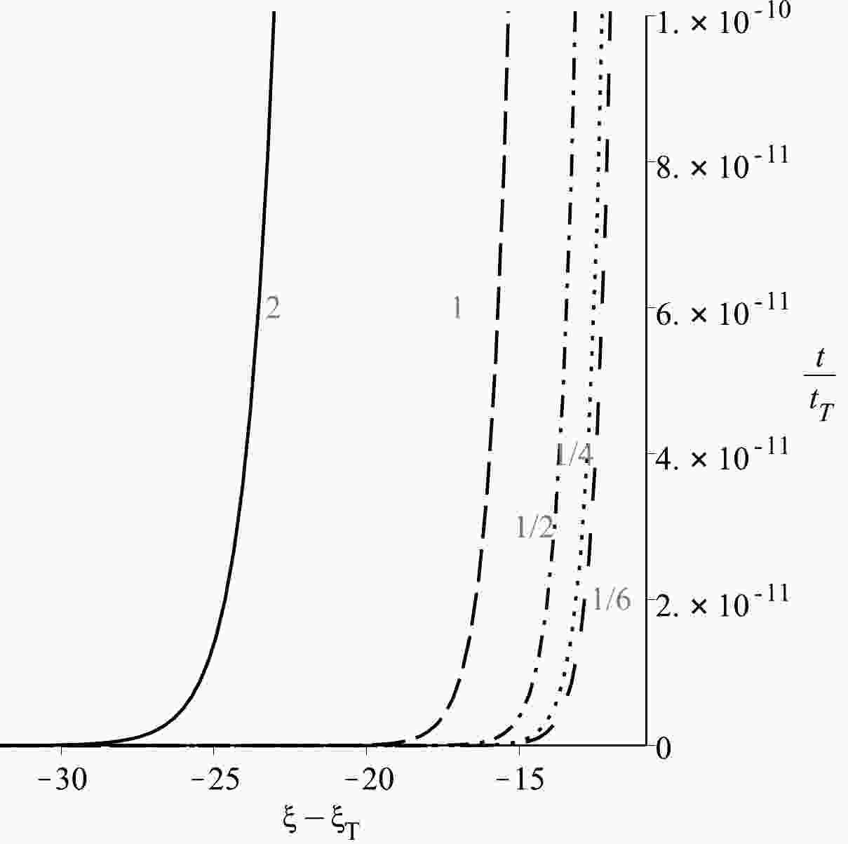
Next, let us assume that inflation terminates at time
$ t_T $ . From Eq. (30), it is evident that$ \xi \rightarrow \xi_0 $ when$ t \rightarrow t_T $ . This implies that when inflation terminates, ξ assumes a constant value. It is clear from Fig. 1 that practically, even when$ t \ll t_T $ , the variation in ξ is negligible, i.e.,$ t_b \ll t_T $ . Therefore, the action given by Eq. (19) reduces to
Figure 1. Variation of the conformal field
$ \xi(t) $ with time t at different values of p.$ S=\frac{1}{2} \int {\rm d}^{4}x \sqrt{-g}\; \left\{\frac{1}{k}{\mathcal{R}}-g^{\alpha\beta} \nabla_{\alpha} \psi \nabla_{\beta}\psi -V(\psi)\right\}, $

(35) where the conformal factor
${\rm e}^{-4\xi}$ in Eq. (19) becomes a constant factor${\rm e}^{-4\xi_T}$ , and hence, it can be consumed by the potential. Thus, after the termination of inflation, one would expect to observe the following two features: (i) the effective cosmological term$\Lambda_{\rm eff}\sim t^{-2}$ decreases in an identical manner to the energy densities of the radiation and matter dominated phases after the inflationary era in the Big Bang model, and (ii) reheating initiates in a manner very similar to that in the conventional inflationary models.One important factor in any model regarding inflation is the number of e-foldings produced by inflation, which is defined as
$ N\equiv \ln \frac{a_T}{a_b} =\int_{t_b}^{t_T} \frac{{\rm d}a}{a}=\int_{t_b}^{t_T} H {\rm d}t, $

(36) where
$ t_b $ and$ t_T $ denote the times at which inflation begins and terminates, respectively, and$ a_b $ and$ a_T $ are the corresponding scale factors.Substituting the solutions of (29) and (30) in Eq. (27), we can obtain
$ \begin{array}{*{20}{l}} N\sim q\ln\left(\dfrac{t_T}{t_b}\right), \end{array} $

(37) where q can be obtained from Eq. (31).
Next, to overcome the smoothness and flatness problems, we must ensure that
$ N>60 $ . Based on Eqs. (31) and (37) and the fact that$ t_b \ll t_T $ and$ \gamma \gg 1 $ , one can understand that this condition can be achieved easily. In this connection, we would like to mention that with a constant value of ψ as$ \gamma \gg 1 $ , it is possible to easily achieve the slow-roll condition, and we explain the smoothness and flatness problems based on this. Here, ξ is a dynamical variable; however, ξ eventually becomes a constant quantity, as is evident from Fig. 1. Hence, Eq. (23) effectively transforms into Eq. (35), and it implies the end of inflation. Therefore, we can explain the end of inflation through the dynamical behavior of ξ. -
In this section, we compare our model results with recent observational data [23–26].
From Eq. (25), we have
$ n_s-1=-\frac{p(p+2)}{\gamma^2}, $

(38) $ r =\frac{8p^2}{\gamma^2}. $

(39) Equations (38) and (39) are plotted in Fig. 2 for different values of p. Essentially, we do not require an explicit value for γ while plotting the variation in
$ n_s $ and r; this is because on considering the ratio, the factor γ cancels out. Thus, we skip the step to opt for any particular value of the parameter.
Figure 2. (color online) Plot of r versus
$ n_s $ for different values of p of the monomial potential (all the coloured lines between$ n_s $ and the extreme right line of the conventional power law inflation). The innermost contour corresponds to the Planck + BICEP2 + Keck Array data, whereas the outermost and middle contours correspond to the Planck + WMAP + BAO data at σ and 2σ confidence limits (CL), respectively.Figure 2 indicates that while the conventional power law inflationary model with exponential potential remains completely outside the region allowed by observational results in the
$ \{r, n_s\} $ space, the present model (Eq. (26)) is in very good agreement with the results reported by Dunkley et al. [23] and Ade et al. [24], and it agrees fairly well with the results reported by Ade et al. [25]) and Akrami et al. [26], along with the highly modified inflationary models. It is worth noting that in the present study, for a minimal coupling scalar field, the power-law potential index must satisfy$ p<4 $ to agree with the observational data reported by Dunkley et al. [23], Ade et al. [24, 25], and Akrami et al. [26]. This is different from the non-minimal coupling scalar field case, for which the power law potential index must satisfy$ p>4 $ [77]. In general, for chaotic inflationary models, the usual convention is the following:$ p \geq 1 $ ; however, in the present model, one can infer that for$ p<1 $ , the latest experimental result can be retrieved particularly well. In this connection, it is worthwhile to mention that the monomial potentials$ V(\psi) = \nu m^4_{Pl} (\psi/m_{Pl})^p $ , as described [see Eq. (24)] by Linde [6], with$ p \geq 2 $ are strongly unfavorable with respect to the$ R^2 $ model. Akrami et al. [26] argued that, for these values, the Bayesian evidence is worse than it was in 2015 owing to the smaller level of tensor modes allowed by BK14 [25]. Notably, models with$ p = 1 $ or$ p = 2/3 $ are more compatible with the data reported by Silverstein and Westphal [78] and McAllister et al. [79, 80]. It is interesting to note that our prescribed value$ p<1 $ agrees well with the second option$ p = 2/3 $ . -
Notably, the conventional PLI with an exponential potential encounters important limitations: the cosmological constant problem, graceful exit problem, and mismatch between the parameters obtained theoretically and recent observational results. Over the years, different inflationary models have been proposed to address some of the cosmological problems. In standard inflationary models, researchers typically use a minimally coupled canonical scalar field with an appropriate potential function. Some of these inflationary models depend on the existence of a large cosmological constant at early times; however, they do not make any predictions regarding its small value at later times.
Based on our model, natural explanations to these drawbacks can be obtained. In our analysis, we probed a single scalar field, termed as an inflaton, and its potential had contributions from different fields in the standard model. Thus, it resulted in a large value of the effective cosmological constant. Here, two metrics in the gravitational and inflaton parts pertain to two different conformal frames. This type of anomalous gravitational coupling of the inflaton has been demonstrated to possess novel features in the inflationary paradigm. We can summarize the main results as follows:
1) In this model, the conformal factor behaves like a dynamical field, and anomalous coupling provides a damping factor, which affects the effective potential. Owing to the decay mechanism, the effective cosmological term reduces with time evolution; hence, the large cosmological constant decreases during the inflationary phase. Thus, the cosmological constant problem in the case of the PLI is suppressed.
2) For a monomial inflaton potential, a set of exact solutions is obtained, resulting in the PLI. From this solution set, we can conclude that inflation terminates at a particular time, and with the evolution of time, the radiation and matter dominated era observed after inflation in the standard hot Big Bang model occurs. Thus, the graceful exit problem can be suppressed.
3) We can effectively describe the inflationary mechanism in terms of
$\Lambda_{\rm eff}\equiv 4\pi\nu m_p^2\gamma^p {\rm e}^{(p-4)\xi}$ . The statefinder parameters$ r' $ and$ s' $ turn out to be constants for the scale factor obtained from the PLI with a monomial potential, as should be the case for acceleration due to a Λ-term.4) We demonstrated that the values of the spectral index and the tensor-to-scalar ratio are in very good agreement with the corresponding observational data. A comparison was made with a non-minimally coupled to scalar field situation.
The conformal transformation approach is used in the present case to introduce a damping term so that the potential of the scalar field tends to decrease, and we can explain the termination of inflation. The power law models of inflation have been ruled out based on current observations, and these are also plagued by the graceful exit problem. Thus, we introduce the conformal transformation technique as a tool to modify the PLI such that the graceful exit problem may be solved owing to the damping factor resulting from the transformation; moreover, the spectral index and tensor-to-scalar ratio also turn out to be in agreement with the corresponding observational data. In addition, a late time Λ-like behavior can be observed in case of the monomial potential to justify the current accelerating phase of the universe. In the present study, we did not consider perturbations of any type; however, this aspect will be covered in future research to present our model within a more concrete physical framework and scenario.
-
Author PP is specially grateful to Prof. Amit Kundu, IIEST, for the encouraging discussion. All the authors are thankful to the anonymous referees for their valuable comments, which have enhanced the quality of the paper.
Studies on modified power law inflation
- Received Date: 2022-09-11
- Available Online: 2023-03-15
Abstract: In this study, we evaluate power law inflation (PLI) with a monomial potential and obtain a novel exact solution. It is well known that the conventional PLI with an exponential potential is inconsistent with the Planck data. Unlike the standard PLI, the present model does not encounter the graceful exit problem, and the results agree fairly well with recent observations. In our analysis, we calculate the spectral index and the tensor-to-scalar ratio, both of which agree very well with recent observational data and are comparable with those of other modified inflationary models. The employed technique reveals that the large cosmological constant decreases with the expansion of the universe in the case of the PLI. The coupling of the inflaton with gravitation is the primary factor in this technique. The basic assumption here is that the two metric tensors in the gravitational and inflaton parts correspond to different conformal frames, which contradicts with the conventional PLI, where the inflaton is directly coupled with the background metric tensor. This fact has direct applications to different dark energy models and the assisted quintessence theory.


 DownLoad: