Using simulated Tianqin gravitational wave data and electromagnetic wave data to study the coincidence problem and Hubble tension problem

The observations of Type Ia supernovae (SNe) suggest that the universe is in a state of accelerated expansion [1–5]. Subsequent observations of the cosmic microwave background (CMB) radiation and large-scale structure have further confirmed this view [6–10]. Consequently, scientists have introduced a negative pressure energy as the driving force for the expansion of the universe; they called it dark energy. At the same time, many dark energy models have been proposed to study the nature of dark energy. Among them, the Λ cold dark matter (ΛCDM) model is the most widely used and agrees with various cosmology observations. However, the ΛCDM model also faces some unresolved theoretical challenges [11, 12], namely the coincidence problem. This problem raises because the present epoch is particularly special: the density of dark energy is of the same order of magnitude as the energy density of matter during this period. In addition, the measurement of $ H_0 $ in Ref. [13] was $74.03 \pm $$ 1.42 ~{\rm kms}^{-1}~{\rm Mpc}^{-1}$ and another measurement of $ H_0 $ was $67.4\pm 0.5 ~{\rm kms}^{-1}~{\rm Mpc}^{-1}$ [7] ; the deviation between these two results is $ 4.4\sigma $. It reflects the problem of measurement inconsistencies between the early and late universes. At present, there are two main directions to solve these problems: one is the use of new models [14–25]; the other is to find a more intuitive cosmological observation to obtain a more accurate Hubble constant, for example by using gravitational wave data to constrain the cosmological model [26–30].

In this study, we used an interaction dark energy model that considers a particular interaction. When we consider the proper interaction of dark energy with dark matter, dark energy can transform into dark matter, which in turn allows dark matter and dark energy to gain some balance, thereby alleviating the problem of coincidence. Some observations also support this idea of interactions. For example, Bertolami et al. [31–34] pointed out that the Abelle group A586 indicates an interaction between dark energy and dark matter. In addition, Abdalla et al. [35, 36] found that optical, X-ray, and weak lens data from the relaxation cluster show signals of energy exchange between them. In addition to proposing a cosmological model, the model itself must be constrained with the parameters of the observed model from various data. Chen et al. [37] limited the model with data from supernovae (SNIa), CMB, and baryon acoustic oscillation (BAO), showing that dark energy interaction with matter was necessary. Cao et al. [38, 39] used a combination of data such as Hubble parametric data and SNIa to constrain the model parameters, and the results showed that the coincidence problem is not alleviated. However, a slight transfer of dark energy to dark matter is expected to be one of the solutions to alleviate the coincidence problem. In a previous study of ours, based on the VLBI observation results of dense structures in 120 medium-luminance radio quasars (QSO), we combined SNIa, CMB, and BAO data [14]. We also investigated the roles of strong gravitational lensing data in the study of dark energy by using measurements of the time-delay effect in 18 strong gravitational lensing systems [40].

In this study, the data we used were simulated gravitational wave (GW) data from Tianqin. Gravitational wave sources from binary bodies are produced together and provide a direct measurement of the luminosity distance. The Tianqin is a space-based GW detector developed by a team at Sun Yat-sen University in China, and its project concept has some unique features [41–46]. The equilateral triangular arm is approximately $ 10^{5} $ km long, and the frequency sensitivity band of the detector overlaps with LISA at approximately $ 10^{4} $ Hz and DECIGO at approximately 0.1 Hz. Owing to its short arm length and better sensitivity than LISA and Taiji in higher frequency bands, Tianqin fills the frequency gap between LISA and DECIGO. In addition, we also used $ H(z) $, SNe, and H0LiCOW data combined with Tianqin data to constrain the model.

The rest of the paper is organized as follows. In Sec. II, we introduce the interaction dark energy model used in this study. In Sec. III, we mainly introduces the gravitational wave data (Tianqin) and electromagnetic wave data (H0LiCOW, $ H(z) $, SNe) used in this study. In Sec. IV, we describe how gravitational wave data and electromagnetic wave data were used to constrain the interacting dark energy model and analyze the results. Finally, in Sec. V, we summarize this paper.

To describe dark energy, we choose a model of interaction between dark energy density and dark matter density. In the flat FRW metric universe, it is assumed that dark energy and dark matter exchange energy through interaction Q [14].

where $ \rho_{X} $ is the density of dark energy and $ \rho_{m} $ is the density of matter. $ H(z)=\dfrac{\dot{a}}{a} $ represents the Hubble parameter, where $ a=1/(1+z) $ and $ \dot{a} $ means derivative with respect to time. In addition, $ \rho_{X} $ and $ \rho_{m} $ have a phenomenological relationship $ \dfrac{\rho_{X}}{\rho_{m}}\varpropto a^{\xi} $, where ξ is the severity of the coincidence problem. Thus, we have the following expression:

where $ \omega_x $ is the equation of state of dark energy, and $ \Omega_{X} $ is the dark energy density parameter expressed as $ \Omega_{X}=(1-\Omega_{m})/[1-\Omega_{m}+\Omega_{m}(1+z)^{\xi}] $.

When $\xi+3\omega_x=0(Q=0)$, no interaction exists between dark energy and dark matter. When $\xi+3\omega_x > 0 (Q < 0)$, dark matter is converted into dark energy and the coincidence problem is not alleviated. When $\xi+3\omega_x < 0 (Q > 0)$, dark energy is converted into dark matter and the coincidence problem can be alleviated [47-49]. The parameterized Friedman equation is expressed as follows:

It is believed that supermassive binary black hole unions constitute a good source of gravitational waves [50], and the Tianqin detector can detect supermassive black holes [51–54]. For these reasons, we simulated 1000 sets of gravitational wave data from the merger of two black holes with a mass of $ 10^3 $ solar masses. The redshift (z) of these data was $ 0\sim15 $. It is important to note that when simulating the gravitational wave data, we adopted the flat ΛCDM model with the matter density parameter set as $ \Omega_m=0.286 $ and the Hubble constant set as $ H_0= \rm 69.6~ kms^{-1}Mpc^{-1} $ with $1$% uncertainty [55].

Tianqin is a typical millihertz frequency gravitational wave observatory. Its main mission is to detect GWs from coalescing supermassive black hole binaries (SMBHBs), inspiral of stellar mass black hole binaries, Galactic ultra-binaries, extreme mass ratio inspirals (EMRIs), and stochastic GW background originating from primordial BHs or cosmic strings [51–54]. SMBHB mergers are the most powerful GW sources [50]. This is why we simulated GW data set of SMBHBs with a mass of $ 10^3M_\odot $ and the redshift z was set in the range of $ 0\sim15 $.

We can obtain an absolute measure of the luminosity distance $ D_{L} $ from the chirping GW signals of inspiral compact binary stars [56]. The so-called chirp mass ($ \mathcal{M}_c $) and luminosity distance ($ D_{L} $) determine the GW strain amplitude. The chirp mass can be obtained from the GW signal's phase position, so it is allowed to extract luminosity distance from the amplitude. The waveform function of GW we used is $ h(f) $:

where the Fourier amplitude $ \mathcal{A} $ is

here the luminosity distance $ D_{L} $ is crucial for our purpose and can be expressed as a function of the redshift in the standard flat ΛCDM cosmological model:

where $\Omega_{M}=0.286,\; \Omega_{\lambda}=0.714$, H₀ = 69.6 kms^-1Mpc^-1. $ M_c=(1+z)(m_{1}m_{2})^{3/5}/(m_{1}+m_{2})^{1/5} $ denotes the observed chirp mass. For Tianqin, $ F_{+} $, $ F_{\times} $ and phase parameters can be found in [50].

Moreover, the one-sided power spectral density (PSD) of the detectors' equivalent strain noise provided by Tianqin is as follows [57, 46]:

where $ L_0 $ is the arm length and $L_0=1.73\times10^5 ~{\rm km}$; the PSD of the position noise is $S_x=10^{-24}~ {\rm m^2/Hz}$ and the PSD of the residual acceleration noise is $S_a=10^{-30} {\rm m^2 s^{-4}/Hz}$.

Combining Eqs. (5), (6), (8), we can obtain the signal-to-noise ratio (SNR) of Tianqin:

where $f_{\rm fin} = {\rm min}(f_{\rm ISCO}, f_{\rm end})$ with GW frequency at the innermost stable circular orbit $f_{ISCO} =1/(6^{3/2}M\pi)$ Hz; the upper cutoff frequency for Tianqin is $f_{\rm end} = 1~{\rm Hz}$; $f_{\rm in} = {\rm max}(f_{\rm low},~ f_{\rm obs})$ with lower cutoff frequency of $f_{\rm low} = 10^{-5}$ Hz; and the initial observation frequency is $f_{\rm obs}=4.15\times10^{-5}(M_c/10^{6}M_\odot)^{-5/8}(T_{\rm obs}/1 {\rm yr})^{-3/8}$ Hz. The observation time $T_{\rm obs}$ is 3 months.

The inherent uncertainty of the measurement $\sigma^{\rm inst}_{D_L}$ and increased uncertainty due to weak lenses $\sigma^{\rm lens}_{D_L}$ jointly determine the uncertainty of the luminosity distance. Therefore, we can calculate the total uncertainty of the measurement $ D_L $ as follows [58, 59]:

In order to limit the model parameters, the $ \chi^{2} $ minimum fitting method was adopted:

where $ D_{L}^{GW} $ is the luminosity distance observed by simulation, $ \sigma_{D_{L}}^{GW} $ is the data error, and $D_{L}^{\rm th}$ can be expressed as follows:

In addition, 580 groups of Ia SNe data were also used in this study [60]. These data generally describe the brightness information of the supernova by distance modulus. The observed values in the data are expressed by the apparent magnitude m and absolute magnitude M as follows:

The theoretical value can also be obtained by the following formula:

The $ \chi^{2} $ minimum fitting method related to the distance modulus can be expressed as follows:

where$ \sigma_{u, i} $ denotes the observation errors of supernovae.

Finally, the 31 Hubble parameter ($ H(z) $) samples from the differential age method were also used [61]. The $ \chi^2 $ minimum fitting method related to Hz parameter data set can be expressed as follows:

The time delay phenomenon of strong gravitational lensing in the late universe is an important cosmological probe that provides a method for measuring the Hubble constant ($ H_{0} $) . The time delay data we used came from the H0LiCOW project ($ H_{0} $ Lenses in COSMOGRAIL's Wellspring) [62–65]. In a strong gravitational lensing system, the source of stars forms multiple observation images under the action of the lens, and these images takes different paths to reach our detector, thus creating a time delay between the images. These data are sensitive to the Hubble constant $ H_{0} $ and therefore can be used as suitable constraint data [64].

The time delay between images located at $ \theta_{i} $ and $ \theta_{j} $ can be expressed as

where τ denotes the dimensionless time of arrival, $ \tau=\dfrac{1}{2}\lvert\theta\lvert^{2}-\theta\cdot\beta $, and β is the location of the source. $ \Delta t_{ij} $ represents the measured value of time delay whereas $ D_{\Delta t} $ is the called time delay distance, which can be expressed as follows:

where $ D_{d} $ and $ D_{s} $ are the angular diameter distances obtained when the redshift is $ z_{d} $ and $ z_{s} $, respectively, and $ D_{ds} $ is the angular diameter distance between the lens and source.

In order to constrain cosmological parameters, we used the least squares fitting method to fit the parameters:

where $D_{\Delta t}^{\rm th}$ is the time-delay distance value that theoretically exists in the cosmological model and$D_{\Delta t}^{\rm obs}$ is the actual measured value whose uncertainty is $ \sigma(i) $.

In this study, we used different combinations of four cosmological data sources, namely Tianqin, H0LiCOW, SNe, and $ H(z) $, to constrain the interaction model. More specifically, they are Tianqin, $ H(z) $+SNe, H0LiCOW, H0LiCOW+SNe+$ H(z) $, and Tiqanqin+H0LiCOW+SNe+$ H(z) $, respectively. The Markov Chain Monte Carlo (MCMC) algorithm and maximum likelihood method were used to limit the interacting dark energy model. For $ \chi^{2} $ values of multiple sets of data, the following formula was used for combination:

In Table 1, we show the constraint results of constraint model parameters ($ \Omega_{m} $, $ \omega_{x} $, ξ, $ H_{0} $) under five different data combinations. Table 2 shows the parameter error estimates obtained under different data combinations calculated as $ \epsilon(p)=\sigma(p)/p $, where p represents the parameter center value in the model and $\sigma(p)= $ $ \sqrt{(\sigma(p)^{2}_{\rm upper}+\sigma(p)^{2}_{\rm lower})/2}$.

Data	$ \Omega_m $	$ \omega_x $	ξ	$ H_0 $
Tianqin	$ 0.40_{-0.17}^{+0.25}(1\sigma) $	$ -1.83_{-0.67}^{+0.67}(1\sigma) $	$ 3.8_{-1.9}^{+0.89}(1\sigma) $	$ 74.4_{-6.0}^{+4.3}(1\sigma) $
H(z)+SNe	$ 0.38_{-0.20}^{+0.20}(1\sigma) $	$ -1.37_{-0.28}^{+0.68}(1\sigma) $	$ 3.39_{-1.6}^{+0.56}(1\sigma) $	$ 69.99_{-0.44}^{+0.44}(1\sigma) $
H0LiCOW	$ 0.284_{-0.27}^{+0.067}(1\sigma) $	$ -1.73_{-0.75}^{+0.21}(1\sigma) $	$ 4.5_{-1.6}^{+5.4}(1\sigma) $	$ 79.6_{-6.7}^{+4.8}(1\sigma) $
H0LiCOW+SNe+H(z)	$ 0.34_{-0.21}^{+0.21}(1\sigma) $	$ -1.26_{-0.22}^{+0.63}(1\sigma) $	$ 3.43_{-1.8}^{+0.54}(1\sigma) $	$ 69.97_{-0.42}^{+0.42}(1\sigma) $
Tianqin+H0LiCOW+SNe+H(z)	$ 0.36_{-0.18}^{+0.18}(1\sigma) $	$ -1.29_{-0.23}^{+0.61}(1\sigma) $	$ 3.15_{-1.1}^{+0.36}(1\sigma) $	$ 70.04_{-0.42}^{+0.42}(1\sigma) $

Table 1.  Parametric results obtained from different data constraint interaction models.

Data	$ \epsilon(\Omega_{m}) $	$ \epsilon(\omega_{x}) $	$ \epsilon(\xi) $	$ \epsilon({H}_{0}) $
Tianqin	$ 0.625(1\sigma) $	$ 0.367(1\sigma) $	$ 0.5(1\sigma) $	$ 0.081(1\sigma) $
H(z)+SNe	$ 0.526(1\sigma) $	$ 0.496(1\sigma) $	$ 0.472(1\sigma) $	$ 0.006(1\sigma) $
H0LiCOW	$ 0.950(1\sigma) $	$ 0.433(1\sigma) $	$ 1.200(1\sigma) $	$ 0.084(1\sigma) $
H0LiCOW+SNe+H(z)	$ 0.617(1\sigma) $	$ 0.500(1\sigma) $	$ 0.524(1\sigma) $	$ 0.006(1\sigma) $
Tianqin+H0LiCOW+SNe+H(z)	$ 0.5(1\sigma) $	$ 0.473(1\sigma) $	$ 0.349(1\sigma) $	$ 0.006(1\sigma) $

Table 2.  Constraint precision of the parameters ($\Omega_m,~ \omega_x,~ \xi,~ H_0$) obtained from different observational data.

As can be seen from Table 1, the Hubble constant ($ H_0 $) values given by the five data combinations with $ 1\sigma $ error are $ {H}_{0}=74.4_{-6.0}^{+4.3}~{\rm kms}^{-1}~{\rm Mpc}^{-1}$, $H_{0}=69.99_{-0.44}^{+0.44} {\rm kms}^{-1}~{\rm Mpc}^{-1}$, $H_{0}=79.6_{-6.7}^{+4.8}~{\rm kms}^{-1}~{\rm Mpc}^{-1}$, $H_{0}=69.97_{-0.42}^{+0.42} $ ${\rm kms}^{-1}~{\rm Mpc}^{-1}$, and$H_{0}=70.04_{-0.42}^{+0.42}~{\rm kms}^{-1}~{\rm Mpc}^{-1}$, respectively. We can see that the values of the Hubble constant $ H_0 $ given by ($ H(z) $+SNe, H0LiCOW+SNe+$ H(z) $, Tianqin+ H0LiCOW+SNe+$ H(z) $) with a confidence interval of $ 1\sigma $ are $H_{0}=69.99_{-0.44}^{+0.44}~{\rm kms}^{-1}~{\rm Mpc}^{-1}$, $H_{0}=69.97_{-0.42}^{+0.42} {\rm kms}^{-1}~{\rm Mpc}^{-1}$, and $H_{0}=70.04_{-0.42}^{+0.42}~{\rm kms}^{-1}~{\rm Mpc}^{-1}$, which are smaller than $H_{0}=74.03_{-1.42}^{+1.42}~{\rm kms}^{-1}~{\rm Mpc}^{-1}$ given by the Hubble Space Telescope (HST) and larger than $H_{0}=67.4_{-0.5}^{+0.5}~{\rm kms}^{-1}~{\rm Mpc}^{-1}$ given by Plank 2018. This indicates that the conflict problem of $ H_0 $ has been alleviated to some extent. However, the center value of $ H_0 $ given by Tianqin and H0LiCOW data is larger than $H_{0}=74.03_{-1.42}^{+1.42}~{\rm kms}^{-1}~{\rm Mpc}^{-1}$ given by the HST, which indicates that the Hubble tension problem has not been alleviated. In addition, we can see from Table 2 that the constraint precision of $ H_0 $ given by the combination of electromagnetic wave data (H0LiCOW+SNe+$ H(z) $) and gravitational wave data (Tianqin) is 0.006 and 0.081, respectively. This means that, in this model, the electromagnetic wave data has a better constraint effect on $ H_0 $ than gravitational wave data. Furthermore, the constraint precision given by Tianqin+H0LiCOW+SNe+$ H(z) $ is 0.006, which further indicates that the constraint effect of gravitational wave data on $ H_0 $ in this model is weak.

In addition, other parameters besides Hubble's constant are listed in Table 1 to analyze the coincidence problem. In the previous content, we mentioned that when $ \xi+3\omega_x=0 $, there is no interaction; when $ \xi+3\omega_x> 0 $, dark matter transitions into dark energy and the coincidence problem is not alleviated; and when $ \xi+3\omega_x<0 $, dark energy transitions into dark matter and the coincidence problem can be alleviated. Note from Table 1 that $ \xi+3\omega_x=-1.69^{+2.9}_{-3.91} $(Tianqin), $ \xi+3\omega_x= -0.35^{+2.43}_{-2.46} $ (H0Li-COW+SNe+$ H(z) $), and $ \xi+3\omega_x = -0.72^{+2.19}_{-1.79} $ (Tianqin+ H0LiCOW+SNe+$ H(z) $). We can clearly see that each of the three data sets (Tianqin, H0LiCOW+SNe+$ H(z) $, Tianqin+H0LiCOW+SNe+$ H(z) $) presents a central value of $ \xi+3\omega_x $ less than 0, which means that the coincidence problem is alleviated, but $ \xi+3\omega_x=0 $ is still within the $ 1\sigma $ error range. In addition, the results for the parameter $ \Omega_{m} $ obtained by the five data constraint models are consistent with those obtained by the CMB data from Planck satellite ($ \Omega_{m}=0.31\pm0.017(1\sigma) $) [66] within an error range of $ 1\sigma $.

In this study, we used 31 groups of Hubble parameter observation data, 6 groups of H0LiCOW data, 580 groups of Type Ia supernova observation data, and 1000 groups of Tianqin simulation data to constrain the parameters of the interacting dark energy model. We used Python programming to calculate data related formulas and implement the MCMC algorithm program. 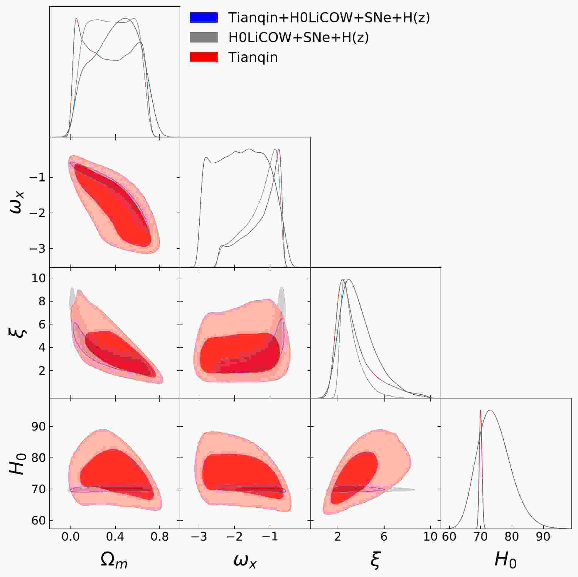The MCMC algorithm was used to calculate the $ \chi^{2} $ test value of the observed data. The constraint results of the observational data on the model parameters and the circle graphs are shown in Table 1 and Fig. 1, respectively.

Figure 1.  (color online) Contour maps of Tianqin, H0LiCOW+SNe+$ H(z) $ and Tianqin+H0LiCOW+SNe+$ H(z) $ data combinations with constraints on model parameters ($ \Omega_m $, $ \omega_x $, ξ, $ H_0 $).

(1) The value of the Hubble constant $ H_0 $ given by ($ H(z) $+SNe, H0LiCOW+SNe+$ H(z) $, Tianqin+H0LiCOW+SNe+$ H(z) $) with a confidence interval of $ 1\sigma $ are $H_{0}=69.99_{-0.44}^{+0.44}~{\rm kms}^{-1}~{\rm Mpc}^{-1}$, $ H_{0}=69.97_{-0.42}^{+0.42} ~{\rm kms}^{-1}~{\rm Mpc}^{-1}$, and $H_{0}=70.04_{-0.42}^{+0.42}~{\rm kms}^{-1}~{\rm Mpc}^{-1}$, respectively. This indicates that the conflict problem of $ H_0 $ has been alleviated to some extent.

(2) With respect to the constraint precision of the Hubble constant ($ H_0 $), we found that the electromagnetic wave data (H0LiCOW+SNe+$ H(z) $) are better than the gravitational wave data for the model parameter $ H_0 $ in this interacting dark energy model.

(3) Based on the constraint results of the different observational data on the parameters ξ and $ \omega_{x} $, we can see that $ \xi+3\omega_x=-1.69^{+2.9}_{-3.91} $(Tianqin), $ \xi+3\omega_x=-0.35^{+2.43}_{-2.46} $(H0LiCOW+SNe+$ H(z) $), and $ \xi+3\omega_x=-0.72^{+2.19}_{-1.79} $(Tianqin+H0LiCOW+SNe+$ H(z) $). This means that both electromagnetic wave data and gravitational wave data can alleviate the coincidence problem to some extent in this model. However, $ \xi+3\omega_x=0 $ is still within a$ 1\sigma $ error range, which indicates that the ΛCDM model is still the model in best agreement with observational data at present.

Finally, given that the Tianqin Gravitational wave detector has not yet detected GWs generated by high-redshift supermassive black hole binaries (SMBHBs), we used GW data with uniform distribution of redshift for simulation. In addition, H0LiCOW and Tianqin data have a weak constraint effect on the model parameters that may be caused by the small H0LiCOW data and unreal gravitational wave data. Therefore, we expect to detect more real gravitational wave data and strong gravitational lensing data in the future to help us further investigate the coincidence and Hubble tension problems.