


 Abstract
 HTML
HTML Reference
 Related
 PDF
PDF


-
Weyl [1] in 1919 and Eddington [2] in 1923included higher order constant terms concerned with the curvature in the action of General Relativity (GR) first introduced by Albert Einstein. We can quantize GR by the non-renormalizability of the theory in a conventional way. Utiyama and De Witt [3] in 1962 showed that we can renormalize GR in one loop if the Einstein-Hilbert (EH) action is constructed with higher-order curvature terms. In addition, when quantum corrections, or string theory, entered into the scenario, the action of effective gravitational field with low energy required higher-order curvature terms [4]. Inspired by this argument, scientists have tried to modify the EH action in applied higher order theories of gravity.
Therefore, higher-orders of Ricci scalar should be incorporated into the action. We should keep in mind that the modified theories of gravity are important at scales only in the range of the Planck scale, i.e., in the newborn universe or at black hole (BH) singularities, e.g., inflation due to curvature case [5]. Sotiriou and Felice [6, 7] reviewed the well-known "
$ f(R) $ theory of gravity." This$ f(R) $ gravity was reconstructed by Dunsby et al. [8] considering the background as Friedman-Lemaitre-Robertson-Walker (FLRW) type. Particularly, the authors predicted the only Lagrangian with a real value for which$ f(R) $ can generate a true Lambda cold dark matter ($ {\Lambda} CDM $ ) expansion for a dust-like matter-filled universe and is equivalent to the EH Lagrangian with a cosmological constant, which is positive. A general formalism was proposed by Mukherjee and Banerjee [9], using which we can observe the later time dynamics of the universe for a given analytic model of$ f(R) $ gravity considering cold dark matter. The outcomes of energy conditions of the$ f(R) $ gravity for various cosmological cases have also been investigated in Ref. [10–14]. The energy conditions using the Raychaudhuri equations in the expanding universe were also studied in Refs. [15–17].Harko and Lobo [18] considered the action as an arbitrary function of not only the Ricci scalar (R) but also the matter Lagrangian (
$ L_{m} $ ). With the help of the metric formalism, the authors achieved the gravitational field equations of$ f(R,L_{m}) $ gravity, along with the equations of motion (EOM) of test particles. Subsequently, Wang et al. [19] achieved the general energy conditions of the$ f(R,L_{m}) $ gravity. In Refs. [20–22], the authors described the power-law cosmic expansion in higher derivative gravity. Harko et al. [23] included the trace of the Stress-energy tensor in the action along with the Ricci scalar and developed a new theory named `$ f(R,T) $ theory'. This type of modified gravity has been extensively used recently to study various cosmological phenomena [24–27].The development of the K-essence model was carried out in Refs. [28–36]. On the basis of the Dirac-Born-Infeld (DBI) model [37–39], Manna et al. [40–42] derived a K-essence emergent gravity metric (
$ \bar G_{\mu\nu} $ ), which has a different significance than the usual gravitational metric,$ g_{\mu\nu} $ . The K-essence model [28–36] is essentially a scalar field theory where the kinetic energy of the K-essence field dominates the potential energy of the field. The Lagrangian corresponding to the K-essence field is of non-canonical type. The difference between K-essence theory, which incorporates non-canonical kinetic parts, and canonical relativistic field theories lies in the non-trivial dynamical solutions of the K-essence EOM. In addition to the spontaneous breaking of Lorentz invariance, it also changes the perturbed metric near the solutions. Hence, these perturbations move along the formal emergent or analogue curved space-time with the perturbed metric. The Lagrangian for the K-essence model can be written as,$ L=-V(\phi)F(X) $ , where ϕ is the K-essence scalar field and$ X=\frac{1}{2}g^{\mu\nu}\nabla_{\mu}\phi\nabla_{\nu}\phi $ [43].A modified version of
$ f(R) $ gravity was also studied by Nojiri et al. [44]. They considered the higher order kinetic terms of a scalar field, which was incorporated in vacuum$ f(R) $ gravity's action part. The authors included a general class of the K-essence Lagrangian,$ G(X) $ with the action of vacuum$ f(R) $ gravity. In the background of slow-roll approximation, the authors investigated the inflationary sides of their theory. Odintsov et al. [45] analyzed the consequences of K-essence geometry in the$ f(R) $ gravity when cold dark matter and radiation are present. Perfect fluids with a similar model were considered in Ref. [44]. Their findings included several cosmological quantities, such as the dark energy equation of state parameter ($ {\omega} $ ), the dark energy density parameter ($ \Omega_d $ ), and some state finder quantities. Recently, Oikonomou et al. [46] discussed the phase space of a simple K-essence$ f(R) $ gravity theory.Next, let us discuss the importance of the K-essence theory with specific choice of the DBI type Lagrangian. It is now unavoidable to admit the acceleration of the universe after analyzing the observations of Large-Scale Structure, type Ia Supernovae's observations, and measurements of anisotropy of Cosmic Microwave Background [47]. It has also been acknowledged that our universe is now dominated by a component named dark energy, which imposes negative pressure. Scientists proposed cosmological constant or vacuum density to be the candidates for such an exotic component of the universe. However, the barrier of the cosmological coincidence problem created hurdles for us and raised the question, "why does the strange dark energy component possess a tiny energy density
$ (O(meV^4 )) $ compared with the simple expectation based on quantum field theory?" Additionally, "the occurrence of the acceleration at such a late stage of evolution" continuously poked cosmologists for better theories. The problem with most of the dark energy models (e.g., cosmological constant) is that they require extraordinary fine tuning of the initial energy density, which is on the order of$ 100 $ or more smaller than the initial matter-energy density.A new model, known as K-essence theory, with a scalar field and excellent dynamic properties that can avoid the long awaited fine-tuning problem has been developed [28]. The most promising feature of this model is that it brings the negative pressure from its nonlinear kinetic energy of the scalar field. It has already been investigated for a wide class of theories. There exist attractor solutions [29, 48] in which the scalar field propagates with different evolution speeds to achieve the required equation of state of the K-essence theory in different epochs with changing background equation of state. While our universe was going through the epoch of radiation domination, K-essence field was dominant, and by imitating the equation of state (EOS) of the radiation, the ratio of K-essence field and radiation density is held constant. At the time of dust domination, the K-essence theory failed to mimic the EOS of dust-like phase for its dynamical characteristics. It also significantly decreased its energy value and settled upon a constant value. Subsequently, the field outgrew the matter density and took the universe into cosmic acceleration at a time roughly corresponding to the current age of the universe. Finally, the EOS of K-essence theory gradually settled to a value between
$ 0 $ and$ -1 $ .The well-known Quintessence Trackers models [49–55] almost give the same result as that of the K-essence theory, but with one problem. Although it can mimic the state equation of matter and radiation for background EOS, it requires an adjustable parameter, which needs to be fine tuned to get the preferable energy density that can produce the negative pressure at present age.
K-essence theory is different in the sense that it traces the background energy density when the universe was in radiation epoch only. The sharp transition of positive pressure to negative pressure at the matter-radiation equality occurs automatically because of its dynamics. K-essence theory was unable to dominate before matter-radiation equality as it was busy tracking the radiation background. Since the energy density inevitably drops to a small value at the transition to dust domination, it is impossible to dominate immediately just after the dust domination. On the other hand, as the matter density drops more rapidly than the energy density with expanding universe, the K-essence field came into control at an age roughly around the current epoch. Thus, the whole Cosmic Coincidence Problem (i.e., why we live in the era of dark matter and dark energy density's equality) vanishes owing to the fact that we came to observe the universe at the right time after matter-radiation equality.
K-essence models also ensures the production of the dark energy component where the sound speed (
$ c_{s} $ ) does not exceed light speed. There exists a difference between these models and scalar field quintessence models from the observational background with a canonical kinetic term (for which$ c_{s} = 1 $ ), and this may be one of the ways to reduce cosmic microwave background (CMB) fluctuations measured on large angular scales [56–58]. Though, there may be some stages where the fluctuations of the field can propagate superluminally ($ c_{s}>1 $ ) [32, 33, 59].Some cosmological behaviors and the stability of the K-essence model in FLRW spacetime has been studied by Yang et al. [60]. Some opposite results have been obtained for small sound speeds of scalar perturbations, which implies clustering of dark energy and an increase in cosmological perturbations [61, 62].
Historically, Born and Infeld [37] introduced a non-canonical kinetic theory to overcome the infinite self-energy of the electron. Some more non-canonical theories were also studied in literature, like [38, 39]. The studies [63–71], focusing on topics such as string theory, brane cosmology, and D-branes have also used the DBI type non-canonical Lagrangian.
Motivated by this importance of the K-essence theory, which prescribes a way to investigate the effects of the presence of the dark energy component in the cosmological framework, in this paper, we study
$ f(R)- $ gravity in the context of K-essence emergent gravity, i.e., dark energy in a general manner. We have made the generalization of the$ f({\bar{R}},L(X)) $ theory with the help of the metric formalism, where$ {\bar{R}} $ is the Ricci scalar of the K-essence geometry and$ L(X) $ is the DBI type non-canonical Lagrangian. Panda et al. [72] modified the$ f(R,T) $ theory in the context of dark energy using the K-essence model. The process of studying these two papers is fundamentally different, i.e., the consideration of actions differs.Further, we have calculated the energy conditions and modified Friedman equations in
$ f({\bar{R}},L(X)) $ gravity and considered the flat FLRW-type metric as the background gravitational metric. The modified field equation, Friedmann equations, and energy conditions for the new$ f({\bar{R}},L(X)) $ gravity theory are different from the usual$ f(R,L_{m}) $ [18] and$ f(R) $ [6] gravity theories. In addition, we have solved the modified Friedmann equations using the power law cosmic expansion method.The remainder of this paper is organized as follows. In Sec. II, we briefly discuss the K-essence emergent geometry based on the following works [30–34, 40–42]. In Sec. III, we formulate
$ f({\bar{R}},L(X)) $ gravity in the context of the K-essence emergent geometry. We also derive the modified field equations and the requirement condition of the energy-momentum tensor conservation in$ f({\bar{R}},L(X)) $ gravity. The modified Friedmann equations are introduced in Sec. IV, considering the background gravitational metric as flat FLRW and the K-essence scalar field as a function of time only. The solution of the Friedmann equations is solved for specific choice of$ f({\bar{R}},L(X)) $ using the power law method in Sec. V, whereas in Sec. VI, we develop the energy conditions and constraints of$ f({\bar{R}},L(X)) $ gravity with an example. The last section, Sec. VII, contains some general discussion and key conclusions of our work. Additionally, we briefly discuss the$ f(R) $ -gravity and$ f(R,L_{m})- $ gravity and corresponding energy conditions [10–14, 19, 73] in the Appendix. -
In this section, we will discuss the development of the modified metric corresponding to the emergent spacetime, which is related with a general background geometry and a very general K-essence scalar field. The K-essence scalar field, ϕ, has action [30–34]
$ \begin{array}{*{20}{l}} S_{k}[\phi,g_{\mu\nu}]= \int {\rm d}^{4}x {\sqrt -g} L(X,\phi), \end{array} $

(1) which has a minimal coupling with the background space-time metric,
$ g_{\mu\nu} $ , and$ X={1\over 2}g^{\mu\nu}\nabla_{\mu}\phi\nabla_{\nu}\phi $ represents the canonical kinetic term. The energy-momentum tensor is$ \begin{aligned}[b] T_{\mu\nu}\equiv & {-2\over \sqrt {-g}}{\delta S_{k}\over \delta g^{\mu\nu}}=-2\frac{{\partial} L}{{\partial} g^{\mu\nu}}+g_{\mu\nu}L \\=&-L_{X}\nabla_{\mu}\phi\nabla_{\nu}\phi+g_{\mu\nu}L, \end{aligned} $

(2) with
$L_{\rm X}= {{\rm d}L\over {\rm d}X},\; L_{{\rm{X}}X}= {{\rm d}^{2}L\over {\rm d}X^{2}},\; L_{\phi}={{\rm d}L\over {\rm d}\phi}$ , and the symbol$ \nabla_{\mu} $ standing for the covariant derivative with respect to the gravitational metric,$ g_{\mu\nu} $ .The EOM of a scalar field is
$ -{1\over \sqrt {-g}}{\delta S_{k}\over \delta \phi}= G^{\mu\nu}\nabla_{\mu}\nabla_{\nu}\phi +2XL_{X\phi}-L_{\phi}=0, $

(3) where
$ G^{\mu\nu}\equiv \frac{c_{s}}{L_{X}^{2}}[L_{X} g^{\mu\nu} + L_{XX} \nabla ^{\mu}\phi\nabla^{\nu}\phi], $

(4) with
$ 1+ {2X L_{XX}\over L_{X}} > 0 $ and$ c_s^{2}(X,\phi)\equiv{(1+2X{L_{XX}\over L_{X}})^{-1}} $ .The inverse metric,
$ G^{\mu\nu} $ , can be written in the following form:$ G_{\mu\nu}={L_{X}\over c_{s}}[g_{\mu\nu}-{c_{s}^{2}}{L_{XX}\over L_{X}}\nabla_{\mu}\phi\nabla_{\nu}\phi]. $

(5) Applying a conformal transformation further [40, 41],
$ \bar G_{\mu\nu}\equiv {c_{s}\over L_{X}}G_{\mu\nu} $ gives$ \bar G_{\mu\nu} ={g_{\mu\nu}-{{L_{XX}}\over {L_{X}+2XL_{XX}}}\nabla_{\mu}\phi\nabla_{\nu}\phi}. $

(6) Using Eq. (2), the effective emergent metrics (6) can be written as [32, 33]
$ \bar G_{\mu\nu}=\left[1-\frac{LL_{XX}}{L_{X}(L_{X}+2XL_{XX})}\right]g_{\mu\nu}+\frac{L_{XX}}{L_{X}(L_{X}+2XL_{XX})}T_{\mu\nu}. $

(7) We should always keep it in mind that,
$ L_{X}\neq 0 $ when$ c_{s}^{2} $ is positive, and only then, Eqs. (1) – (4) will yield meaningful physics.Evidently, if ϕ has a non-trivial space-time configuration, then usually the emergent metric,
$ \bar G_{\mu\nu} $ , is not conformally equivalent to$ g_{\mu\nu} $ . So ϕ has dissimilar characteristics as ompared with canonical scalar fields with the locally defined causal structure. Further, if there is no explicit dependency of L on ϕ, the reformed EOM (3) becomes$ -{1\over \sqrt {-g}}{\delta S_{k}\over \delta \phi} = \bar G^{\mu\nu}\nabla_{\mu}\nabla_{\nu}\phi=0. $

(8) The authors [33, 34, 37–42, 74] take the Dirac-Born-Infeld (DBI) type non-canonical Lagrangian as
$ L(X,\phi)=V(\phi)[ 1-\sqrt{1-2X}] $ , where$ V(\phi) $ is a constant potential and kinetic energy of the K-essence scalar field and is much greater than the potential part of the Lagrangian. In this article, we choose the DBI type non-canonical Lagrangian to be an explicit function of X only as$ L(X,\phi)\simeq L(X) $ [43], without any loss of generality and dimensionality since in the K-essence theory, the kinetic energy dominates over the potential energy of the system. Therefore, we can write the Lagrangian as$ \begin{array}{*{20}{l}} L(X,\phi)\simeq L(X)= V\big[1-\sqrt{1-2X}\big], \end{array} $

(9) where V is a constant potential term.
Then
$ c_{s}^{2}(X,\phi)=1-2X $ , and hence, the effective emergent metric (6) turns out to be$ \begin{array}{*{20}{l}} \bar G_{\mu\nu}= g_{\mu\nu} - \nabla_{\mu}\phi\nabla_{\nu}\phi\equiv g_{\mu\nu} - {\partial}_{\mu}\phi{\partial}_{\nu}\phi, \end{array} $

(10) since ϕ is a scalar.
Eqs. (2) and (10) can be rewritten in terms of
$ T_{\mu\nu} $ and$ \nabla_{\mu}\phi $ as$ \begin{array}{*{20}{l}} \bar G_{\mu\nu}L =L_{X}\nabla_{\mu}\phi\nabla_{\nu}\phi+T_{\mu\nu}-L\nabla_{\mu}\phi\nabla_{\nu}\phi. \end{array} $

(11) Following [40, 75], the relation between the new Christoffel symbols and the old ones is
$ \begin{aligned}[b] \bar\Gamma ^{\alpha}_{\mu\nu} =&\Gamma ^{\alpha}_{\mu\nu} + (1-2X)^{-1/2}\bar{G}^{\alpha\gamma}\\&\times[\bar{G}_{\mu\gamma}\partial_{\nu}(1-2X)^{1/2} +\bar{G}_{\nu\gamma}\partial_{\mu}(1-2X)^{1/2}-\bar{G}_{\mu\nu}\partial_{\gamma}(1-2X)^{1/2}]\\ =&\Gamma ^{\alpha}_{\mu\nu} -\frac {1}{2(1-2X)}[\delta^{\alpha}_{\mu}\partial_{\nu}X + \delta^{\alpha}_{\mu}\partial_{\nu}X]. \end{aligned} $

(12) Therefore, using the new Christoffel connections,
$ \bar\Gamma $ , the geodesic equation for the K-essence becomes$ \frac {{\rm d}^{2}x^{\alpha}}{{\rm d}{\lambda}^{2}} + \bar\Gamma ^{\alpha}_{\mu\nu}\frac {{\rm d}x^{\mu}}{{\rm d}{\lambda}}\frac {{\rm d}x^{\nu}}{{\rm d}{\lambda}}=0, $

(13) where
$ {\lambda} $ is an affine parameter.Now introducing the covariant derivative,
$ D_{\mu} $ [32, 33], corresponding to the emergent metric$ \bar G_{\mu\nu} $ $ (D_{{\alpha}}\bar G^{{\alpha}{\beta}}=0) $ as$ \begin{array}{*{20}{l}} D_{\mu}A_{\nu}={\partial}_{\mu} A_{\nu}-\bar \Gamma^{{\lambda}}_{\mu\nu}A_{{\lambda}}, \end{array} $

(14) and the inverse of the emergent metric is
$ \bar G^{\mu\nu} $ such that$ \bar G_{\mu{\lambda}}\bar G^{{\lambda}\nu}=\delta^{\nu}_{\mu} $ .Ultimately, the "emergent" Einstein's equation becomes
$ \bar{E}_{\mu\nu}={\bar{R}}_{\mu\nu}-\frac{1}{2}\bar{G}_{\mu\nu}{\bar{R}}={\kappa} T_{\mu\nu}, $

(15) where
$ {\kappa}=8\pi G $ is a constant,$ {\bar{R}}_{\mu\nu} $ is emergent gravity's Ricci tensor, and${\bar{R}}(={\bar{R}}_{\mu\nu}\bar{G}^{\mu\nu}) $ is the Ricci scalar of the emergent space-time. -
We now consider the action of modified gravity in the context of K-essence emergent space-time, which takes the following form (
$ {\kappa}=1 $ )$ S= \int {\rm d}^{4}x \sqrt{-\bar{G}}\; f({\bar{R}},L(X)), $

(16) where
$ f({\bar{R}},L(X)) $ is an arbitrary function of the Ricci scalar$ {\bar{R}} $ , the non-canonical Lagrangian density,$ L(X) $ , corresponding to the K-essence theory, and$ \sqrt{-{\bar{G}}}=\sqrt{-{\rm det}({{\bar{G}}_{\mu\nu}})}. $

Based on the following work [18], varying the action, S, with respect to the K-essence emergent gravity metric,
$ \bar{G}^{\mu\nu} $ , we obtain$ \begin{aligned}[b] \delta S =& \int \Bigg[f_{{\bar{R}}}({\bar{R}}, L)\delta {\bar{R}} + f_{L}({\bar{R}}, L)\frac{\delta L}{\delta \bar{G}^{\mu\nu}}\delta \bar{G}^{\mu\nu}\\&- \frac{1}{2}\bar{G}_{\mu\nu}f({\bar{R}}, L)\delta \bar{G}^{\mu\nu} \Bigg] \times\sqrt{-\bar{G}}\; {\rm d}^{4}x, \end{aligned} $

(17) where we have denoted
$ f_{{\bar{R}}}({\bar{R}}, L)=\frac{{\partial}{f({\bar{R}}, L)}}{{\partial} {\bar{R}}} $ and$ f_{L}({\bar{R}}, L)= \frac{{\partial}{f({\bar{R}}, L)}}{{\partial} L} $ .Now, we obtain the variation of the Ricci scalar for the K-essence emergent gravity metric
$ \begin{aligned}[b] \delta {\bar{R}} =& \delta ({\bar{R}}_{\mu\nu}\bar{G}^{\mu\nu}) = \delta {\bar{R}}_{\mu\nu}\bar{G}^{\mu\nu} + {\bar{R}}_{\mu\nu}\delta \bar{G}^{\mu\nu}\\ =&{\bar{R}}_{\mu\nu}\delta \bar{G}^{\mu\nu}+{\bar{G}}^{\mu\nu}(D_{{\lambda}}\delta\bar{\Gamma}^{{\lambda}}_{\mu\nu}-D_{\nu}\delta\bar{\Gamma}^{{\lambda}}_{\mu{\lambda}}), \end{aligned} $

(18) where
$ \begin{array}{*{20}{l}} {\bar{R}}_{\mu\nu} = \partial_{\mu}\bar{\Gamma}^{\alpha}_{\alpha\nu} - \partial_{\alpha}\bar{\Gamma}^{\alpha}_{\mu\nu} + \bar{\Gamma}^{\alpha}_{\beta\mu}\bar{\Gamma}^{\beta}_{\alpha\nu} - \bar{\Gamma}^{\alpha}_{\alpha\beta}\bar{\Gamma}^{\beta}_{\mu\nu}, \end{array} $

(19) $ \bar{\Gamma}^{\alpha}_{\mu\nu} = \frac{1}{2}\bar{G}^{\alpha\beta}[\partial_{\mu}\bar{G}_{\beta\nu} + \partial_{\nu}\bar{G}_{\mu\beta} - \partial_{\beta}\bar{G}_{\mu\nu}], $

(20) and the variation of
$ \delta\bar{\Gamma}^{{\lambda}}_{\mu\nu} $ is$ \delta\bar{\Gamma}^{{\lambda}}_{\mu\nu}=\frac{1}{2}{\bar{G}}^{{\lambda}{\alpha}}[D_{\mu}{\delta}{\bar{G}}_{\nu{\alpha}}+D_{\nu}{\delta}{\bar{G}}_{\mu{\alpha}}-D_{{\alpha}}{\delta}{\bar{G}}_{\mu\nu}]. $

(21) Thus, the expression for the variation of the Ricci scalar,
$ {\delta}{\bar{R}} $ , is$ \begin{array}{*{20}{l}} {\delta}{\bar{R}}={\bar{R}}_{\mu\nu}{\delta}{\bar{G}}^{\mu\nu}+{\bar{G}}_{\mu\nu}D_{{\alpha}}D^{{\alpha}}{\delta}{\bar{G}}^{\mu\nu}-D_{\mu}D_{\nu}{\delta}{\bar{G}}^{\mu\nu}. \end{array} $

(22) Therefore, variation of Eq. (17) is
$ \begin{aligned}[b] \delta S=& \int \Big[f_{{\bar{R}}}({\bar{R}}, L){\bar{R}}_{\mu\nu}\delta \bar{G}^{\mu\nu} + f_{{\bar{R}}}({\bar{R}}, L)\bar{G}_{\mu\nu}D_{{\alpha}}D^{{\alpha}}\delta \bar{G}^{\mu\nu}\\&- f_{{\bar{R}}}({\bar{R}}, L)D_{\mu}D_{\nu}\delta \bar{G}^{\mu\nu} + f_{L}({\bar{R}}, L)\frac{\delta L}{\delta \bar{G}^{\mu\nu}}\delta \bar{G}^{\mu\nu}\\&- \frac{1}{2}\bar{G}_{\mu\nu}f({\bar{R}}, L)\delta \bar{G}^{\mu\nu}\Big]\sqrt{-\bar{G}}d^{4}x.\; \; \; \; \; \end{aligned} $

(23) After partially integrating second and third terms of the above Eq. (23), we get
$ \begin{aligned}[b] \delta S =& \int \Big[f_{{\bar{R}}}({\bar{R}}, L){\bar{R}}_{\mu\nu} + \bar{G}_{\mu\nu}D_{\mu}D^{\mu}f_{{\bar{R}}}({\bar{R}}, L) \\&- D_{\mu}D_{\nu}f_{{\bar{R}}}({\bar{R}}, L) + f_{L}({\bar{R}}, L)\frac{\delta L}{\delta \bar{G}^{\mu\nu}} \\&- \frac{1}{2}\bar{G}_{\mu\nu}f({\bar{R}}, L)\Big]\delta \bar{G}^{\mu\nu}\sqrt{-\bar{G}}{\rm d}^{4}x. \end{aligned} $

(24) Therefore, using the principle of least action, i.e.
$ \delta S = 0 $ , we have the modified field equation for$ f({\bar{R}}, L(X)) $ theory$ \begin{aligned}[b] &f_{{\bar{R}}}({\bar{R}}, L){\bar{R}}_{\mu\nu} + \bar{G}_{\mu\nu}D_{{\alpha}}D^{{\alpha}}f_{{\bar{R}}}({\bar{R}}, L) - D_{\mu}D_{\nu}f_{{\bar{R}}}({\bar{R}}, L) \\&\quad- \frac{1}{2}\bar{G}_{\mu\nu}f({\bar{R}}, L) + f_{L}({\bar{R}}, L)\frac{\delta L}{\delta \bar{G}^{\mu\nu}} = 0. \end{aligned} $

(25) Now, we evaluate the term
$ \frac{\delta L}{\delta \bar{G}^{\mu\nu}} $ as$ \frac{\delta L}{\delta \bar{G}^{\mu\nu}}=\frac{{\delta} L}{{\delta} X}\frac{{\delta} X}{{\delta} g^{\mu\nu}}\frac{{\delta} g^{\mu\nu}}{{\delta}{\bar{G}}^{\mu\nu}}=\frac{1}{2}L_{X}D_{\mu}\phi D_{\nu}\phi(1+D_{{\alpha}}\phi D^{{\alpha}}\phi), $

(26) since for the scalar field
$ \nabla_{\mu}\phi\equiv{\partial}_{\mu}\phi\equiv D_{\mu}\phi $ .Using Eqs. (11), (25), and (26), we obtain the expression for the modified field equation for the
$ f({\bar{R}}, L(X)) $ theory in terms of$ T_{\mu\nu} $ as$ \begin{aligned}[b] &f_{{\bar{R}}}({\bar{R}}, L){\bar{R}}_{\mu\nu} +\left(\bar{G}_{\mu\nu}{\bar{\square}} - D_{\mu}D_{\nu}\right)f_{{\bar{R}}}({\bar{R}}, L)\\&- \frac{1}{2}\left [f({\bar{R}}, L)-Lf_{L}({\bar{R}}, L)(1+D_{{\alpha}}\phi D^{{\alpha}}\phi)\right]\bar{G}_{\mu\nu}\\ &+\frac{1}{2}Lf_{L}({\bar{R}}, L)D_{\mu}\phi D_{\nu}\phi\left[1+D_{{\alpha}}\phi D^{{\alpha}}\phi\right] \end{aligned} $

$ \begin{aligned}[b] \quad=\frac{1}{2}f_{L}({\bar{R}}, L)T_{\mu\nu}\left[1+D_{{\alpha}}\phi D^{{\alpha}}\phi\right]=\frac{1}{2}f_{L}({\bar{R}}, L){\bar{T}}_{\mu\nu},\; \; \; \; \end{aligned} $

(27) where
$ {\bar{\square}}=D_{\mu}D^{\mu} $ and$ {\bar{T}}_{\mu\nu}=T_{\mu\nu}[1+D_{{\alpha}}\phi D^{{\alpha}}\phi] $ .The above Eq. (27) is different from the usual Eq. (104) of
$ f(R,L_{m}) $ theory in the presence of the K-essence scalar field (vide the Appendix). If we consider the emergent gravity metric,$ {\bar{G}}_{\mu\nu} $ , is conformally equivalent to the gravitational metric,$ g_{\mu\nu} $ , and L can be matter Lagrangian, then we get back to the usual$ f(R,L_{m}) $ theory in the absence of the K-essence scalar field. Further, if we consider$ f({\bar{R}},L(X))\equiv f(R,L_{m})\equiv \frac{1}{2}R+L_{m} $ , i.e., the Hilbert-Einstein Lagrangian form, then from Eq. (27), we lead to the standard Einstein field equation$ R_{\mu\nu}-\frac{1}{2}g_{\mu\nu}R=T_{\mu\nu} $ .Contracting the above field equation, Eq. (27), with
$ {\bar{G}}^{\mu\nu} $ , we have the modified trace equation for the$ f({\bar{R}}, L(X)) $ theory as$ \begin{aligned}[b] f_{{\bar{R}}}({\bar{R}}, L){\bar{R}} + 3{\bar{\square}} f_{{\bar{R}}}({\bar{R}}, L)-2\Big[f({\bar{R}}, L)-f_{L}({\bar{R}}, L)L(1+D_{{\alpha}}\phi D^{{\alpha}}\phi)\Big]+\frac{1}{2}Lf_{L}({\bar{R}}, L)D_{\mu}\phi D^{\mu}\phi[1+D_{{\alpha}}\phi D^{{\alpha}}\phi]=\frac{1}{2}f_{L}({\bar{R}}, L){\bar{T}}, \\ \end{aligned} $ 
(28) where
$ {\bar{T}}={\bar{T}}^{\mu}_{\mu} $ is trace of the energy-momentum tensor.Subtracting Eq.
$ (28)\times {\bar{G}}_{\mu\nu} $ from Eq.$ (27)\times 3 $ , we get$ \begin{aligned}[b] &f_{{\bar{R}}}({\bar{R}}, L)({\bar{R}}_{\mu\nu}-\frac{1}{3}{\bar{G}}_{\mu\nu}{\bar{R}})+\frac{1}{6}{\bar{G}}_{\mu\nu}[f({\bar{R}}, L)-Lf_{L}({\bar{R}}, L)(1+D_{{\alpha}}\phi D^{{\alpha}}\phi)]+\frac{1}{3}Lf_{L}({\bar{R}}, L)D_{\mu}\phi D_{\nu}\phi[1+D_{{\alpha}}\phi D^{{\alpha}}\phi]\\=&\frac{1}{2}f_{L}({\bar{R}}, L)({\bar{T}}_{\mu\nu}-\frac{1}{3}{\bar{G}}_{\mu\nu}{\bar{T}})+D_{\mu}D_{\nu}f_{{\bar{R}}}({\bar{R}}, L), \end{aligned} $

(29) which is an another form of the modified field equation in the presence of the K-essence scalar field, ϕ.
By taking covariant divergence with respect to
$ D^{\mu} $ of Eq. (27), we have$ \begin{aligned}[b] &D^{\mu}\Big[f_{{\bar{R}}}({\bar{R}}, L)\Big]{\bar{R}}_{\mu\nu}-({\bar{\square}} D_{\nu}-D_{\nu}{\bar{\square}})f_{{\bar{R}}}({\bar{R}}, L)+f_{{\bar{R}}}({\bar{R}}, L)D^{\mu}\Big({\bar{R}}_{\mu\nu}-\frac{1}{2}{\bar{G}}_{\mu\nu}{\bar{R}}\Big)+\frac{1}{2}{\bar{G}}_{\mu\nu}f_{{\bar{R}}}({\bar{R}},L)D^{\mu}({\bar{R}})\\&-\frac{1}{2}D^{\mu}\Big[f({\bar{R}},L)\Big]{\bar{G}}_{\mu\nu}+\frac{1}{2}D^{\mu}\Big[Lf_{L}({\bar{R}}, L)(1+D_{{\alpha}}\phi D^{{\alpha}}\phi)\Big]{\bar{G}}_{\mu\nu} +\frac{1}{2}D^{\mu}\Big[Lf_{L}({\bar{R}}, L)D_{\mu}\phi D_{\nu}\phi(1+D_{{\alpha}}\phi D^{{\alpha}}\phi)\Big]\\=&\frac{1}{2}D^{\mu}\Big[f_{L}({\bar{R}}, L){\bar{T}}_{\mu\nu}\Big]. \end{aligned} $

(30) Using identities on purely geometrical grounds [76–78] ,
$ D^{\mu}({\bar{R}}_{\mu\nu}-\frac{1}{2}{\bar{G}}_{\mu\nu}{\bar{R}})=D^{\mu}\bar{E}_{\mu\nu}=0 $ ,$ D^{\mu}[f_{{\bar{R}}}({\bar{R}}, L)]{\bar{R}}_{\mu\nu}= ({\bar{\square}} D_{\nu}- D_{\nu}{\bar{\square}})f_{{\bar{R}}}({\bar{R}}, L) $ , and also Eqs. (11) and (26), the above Eq. (30) becomes$ \begin{aligned}[b] D^{\mu}[f_{L}({\bar{R}}, L){\bar{T}}_{\mu\nu}]=&-f_{L}({\bar{R}}, L)D^{\mu}[{\bar{G}}_{\mu\nu}L] +D^{\mu}\left[Lf_{L}({\bar{R}}, L)(1+D_{{\alpha}}\phi D^{{\alpha}}\phi)({\bar{G}}_{\mu\nu}+D_{\mu}\phi D_{\nu}\phi)\right]\\ &\Rightarrow D^{\mu}{\bar{T}}_{\mu\nu}=D^{\mu}\; {\rm ln}[f_{L}({\bar{R}},L)]\times\left[L_{X}D_{\mu}\phi D_{\nu}\phi (1+D_{{\alpha}}\phi D^{{\alpha}}\phi)\right]+D^{\mu}\left[L D_{\mu}\phi D_{\nu}\phi (1+D_{{\alpha}}\phi D^{{\alpha}}\phi)+L{\bar{G}}_{\mu\nu}D_{{\alpha}}\phi D^{{\alpha}}\phi\right]\\ &\Rightarrow D^{\mu}{\bar{T}}_{\mu\nu}=2D^{\mu}\; {\rm ln}[f_{L}({\bar{R}},L)]\frac{\delta L}{\delta {\bar{G}}^{\mu\nu}}+D^{\mu}\left[L D_{\mu}\phi D_{\nu}\phi (1+D_{{\alpha}}\phi D^{{\alpha}}\phi)+L{\bar{G}}_{\mu\nu}D_{{\alpha}}\phi D^{{\alpha}}\phi\right]. \end{aligned} $

(31) Thus, the requirement of the conservation of the energy-momentum tensor
$ (D^{\mu}{\bar{T}}_{\mu\nu}=0) $ for the K-essence Lagrangian, gives an effective functional relation as$ \begin{array}{*{20}{l}} 2D^{\mu}\; {\rm ln}[f_{L}({\bar{R}},L)]\frac{\delta L}{\delta {\bar{G}}^{\mu\nu}}+D^{\mu}\Big[L D_{\mu}\phi D_{\nu}\phi (1+D_{{\alpha}}\phi D^{{\alpha}}\phi)+L{\bar{G}}_{\mu\nu}D_{{\alpha}}\phi D^{{\alpha}}\phi\Big]=0. \end{array} $

(32) -
We consider the gravitational metric,
$ g_{\mu\nu} $ , to be a flat Friedmann-Lemaître-Robertson-Walker (FLRW) metric and the line element for this is$ {\rm d}s^{2}={\rm d}t^{2}-a^{2}(t)\displaystyle\sum\limits_{i=1}^{3} ({\rm d}x^{i})^{2}, $

(33) with
$ a(t) $ being the scale factor, as usual.From Eq. (10), we have the components of the emergent gravity metric as
$ {\bar{G}}_{00}=(1-\dot\phi^{2})\; ;\; {\bar{G}}_{ii}=-[a^{2}(t)+(\phi^{'})^{2}]\; ;\; {\bar{G}}_{0i}=-\dot\phi \phi^{'}={\bar{G}}_{i0}, $

(34) where we consider
$ \phi\equiv \phi(t,x^{i}) $ ,$ \dot\phi=\frac{{\partial} \phi}{{\partial} t} $ , and$ \phi^{'}=\frac{{\partial} \phi}{{\partial} x^{i}} $ .So, the line element of the FLRW emergent gravity metric is
$ {\rm d}S^{2}=(1-\dot\phi^{2}){\rm d}t^{2}-\big[a^{2}(t)+(\phi^{'})^{2}\big]\displaystyle\sum\limits_{i=1}^{3} ({\rm d}x^{i})^{2}-2\dot\phi \phi^{'}{\rm d}t {\rm d}x^{i}. $

(35) Now, from the emergent gravity equation of motion, Eq. (8), we have
$ \begin{aligned}[b] &{\bar{G}}^{00}({\partial}_{0}{\partial}_{0}\phi-{\Gamma}^{0}_{00}{\partial}_{0}\phi-{\Gamma}^{i}_{00}{\partial}_{i}\phi)+{\bar{G}}^{ii}({\partial}_{i}{\partial}_{i}\phi\\&\quad-{\Gamma}^{0}_{ii}{\partial}_{0}\phi-{\Gamma}^{i}_{ii}{\partial}_{i}\phi)+{\bar{G}}^{0i}({\partial}_{0}{\partial}_{i}\phi-{\Gamma}^{0}_{0i}{\partial}_{0}\phi-{\Gamma}^{i}_{oi}{\partial}_{i}\phi) \\&\quad+{\bar{G}}^{i0}({\partial}_{i}{\partial}_{0}\phi-{\Gamma}^{0}_{i0}{\partial}_{0}\phi-{\Gamma}^{i}_{i0}{\partial}_{i}\phi)=0. \end{aligned} $

(36) For simplification, we consider the homogeneous K-essence scalar field, ϕ, i.e.,
$ \phi(t,x^{i})\equiv\phi(t) $ then$ {\bar{G}}_{00}=(1-\dot\phi^{2}) $ ,$ {\bar{G}}_{0i}={\bar{G}}_{i0}=0={\partial}_{i}\phi $ ,$ {\bar{G}}_{ii}=-a^{2}(t) $ , and$ X={1\over 2}g^{\mu\nu}\nabla_{\mu}\phi\nabla_{\nu}\phi=\frac{1}{2}\dot\phi^{2} $ . This consideration is possible in this case, since the dynamical solutions of the K-essence scalar fields spontaneously break Lorentz symmetry. Therefore, the flat FLRW emergent gravity line element (35) and the equation of motion (36) become$ {\rm d}S^{2}=(1-\dot\phi^{2}){\rm d}t^{2}-a^{2}(t)\displaystyle\sum\limits_{i=1}^{3} ({\rm d}x^{i})^{2}, $

(37) and
$ \frac{\dot a}{a}=H(t)=-\frac{\ddot\phi}{\dot\phi(1-\dot\phi^{2})}, $

(38) where
$ H(t)=\frac{\dot a}{a} $ is the usual Hubble parameter (always$ \dot a\neq 0 $ ). Eq. (38) gives the relation between the Hubble parameter and the time derivatives of the K-essence scalar field. Note that in the above spacetime, Eq. (37) always is$ \dot\phi^{2}<1 $ . If$ \dot\phi^{2}>1 $ , the signature of this spacetime will be ill-defined. Moreover, the$ \dot\phi^{2}\neq 0 $ condition holds, instead of$ \dot\phi^{2}=0 $ , which leads to non-applicability of the K-essence theory. Additionally,$ \dot\phi^{2}\neq 1 $ because$\Omega_{\rm matter} + \Omega_{\rm radiation} + \Omega_{\rm dark energy}= 1$ and we can measure$ \dot\phi^{2} $ as dark energy density in units of the critical density, i.e., it is nothing but$\Omega_{\rm dark energy}$ [40–42, 74]. Therefore$ \dot\phi^{2} $ takes a value between$ 0 $ and$ 1 $ .The Ricci tensors and Ricci scalar of the emergent gravity space-time are
$ \begin{aligned}[b] {\bar{R}}_{ii}=&-\frac{a^{2}}{1-\dot\phi^{2}}\left[\frac{\ddot a}{a}+2\left(\frac{\dot a}{a}\right)^{2}+\frac{\dot a}{a}\frac{\dot\phi \ddot\phi}{1-\dot\phi^{2}}\right]\\=&-\frac{a^{2}}{1-\dot\phi^{2}}\left[\frac{\ddot a}{a}+\left(\frac{\dot a}{a}\right)^{2}(2-\dot\phi^{2})\right]\\=&-\frac{a^{2}}{1-\dot\phi^{2}}\left[\dot H+H^{2}(3-\dot\phi^{2})\right], \end{aligned} $

(39) $ \begin{aligned}[b] {\bar{R}}_{00}=&3\frac{\ddot a}{a}+3\frac{\dot a}{a}\frac{\dot\phi \ddot\phi}{1-\dot\phi^{2}} =3\frac{\ddot a}{a}+3\left(\frac{\dot a}{a}\right)^{2}\dot\phi^{2}\\=&3\left[\dot H+H^{2}(1-\dot\phi^{2})\right], \end{aligned} $

(40) and
$ \begin{aligned}[b] {\bar{R}} =& \frac{6}{1-\dot\phi^{2}}\left[\frac{\ddot a}{a}+\left(\frac{\dot a}{a}\right)^{2}+\frac{\dot a}{a}\frac{\dot\phi \ddot\phi}{1-\dot\phi^{2}}\right]\\=& \frac{6}{1-\dot\phi^{2}}\left[\frac{\ddot a}{a}+\left(\frac{\dot a}{a}\right)^{2}(1-\dot\phi^{2})\right]\\ =& \frac{6}{1-\dot\phi^{2}}\left[\dot H +H^{2}(2-\dot\phi^{2})\right], \end{aligned} $

(41) where we have used the relation Eq. (38) and
$ \dot H\equiv\frac{{\partial} H}{{\partial} t}=\frac{a\ddot{a}-\dot{a}^{2}}{a^{2}} $ .Combining Eqs. (39) and (40) with (41), we get
$ {\bar{R}}_{00}=\frac{1}{2}(1-\dot\phi^{2}){\bar{R}}-3H^{2}, $

(42) $ {\bar{R}}_{ii}=-\frac{a^{2}}{(1-\dot\phi^{2})}\left[\frac{1}{6}{\bar{R}}(1-\dot\phi^{2})+H^{2}\right]. $

(43) We assume that the energy-momentum tensor is an ideal fluid type, which is
$ \begin{aligned}[b] T_{\mu}^{\nu}=&diag(\rho,-p,-p,-p)=(\rho +p)u_{\mu}u^{\nu}-\delta_{\mu}^{\nu} p\\ T_{\mu\nu}=&{\bar{G}}_{\mu{\alpha}}T^{{\alpha}}_{\nu}, \end{aligned} $

(44) where p is the pressure and ρ is the matter density of the cosmic fluid. In the comoving frame, we have
$ u^{0}=1 $ and$ u^{{\alpha}}=0 $ ;$ {\alpha}= 1, 2, 3 $ in the K-essence emergent gravity spacetime.Now, the question is whether this type of energy-momentum tensor is valid or not in the case of a perfect fluid model when the kinetic energy (
$ \dot\phi^{2} $ ) of the K-essence scalar field is present. The answer is "yes" since our Lagrangian is$ L(X) = 1-\sqrt{1-2X} $ . This class of models is equivalent to perfect fluid models with zero vorticity, and the pressure (Lagrangian) can be expressed through the energy density only [33, 74].Now, we evaluate the
$ ii $ and$ 00 $ components of the modified field equation (Eq. 27) using Eq. (44) and considering$ \phi\equiv\phi(t) $ only:$ \begin{aligned}[b]& F{\bar{R}}_{ii} + (\bar{G}_{ii}{\bar{\square}} - D_{i}D_{i})F - \frac{1}{2}[f-Lf_{L}(1+\dot\phi^{2})]\bar{G}_{ii}\\ =&\frac{1}{2}f_{L}a^{2}(t)\bar{p}\; \; \; \; \end{aligned} $

(45) and
$ \begin{aligned}[b]& F{\bar{R}}_{00} + (\bar{G}_{00}{\bar{\square}} - D_{0}D_{0})F - \frac{1}{2}[f-Lf_{L}(1+\dot\phi^{2})]{\bar{G}}_{00} \\&\quad+\frac{1}{2}Lf_{L}\dot\phi^{2}(1+\dot\phi^{2}) =\frac{1}{2}f_{L}(1-\dot\phi^{2})\bar{\rho}, \end{aligned} $

(46) with
$ F=f_{{\bar{R}}}({\bar{R}},L)\equiv\dfrac{{\partial} f({\bar{R}},L)}{{\partial} {\bar{R}}} $ ,$ \bar{p}=p(1+\dot\phi^{2}) $ , and$ \bar{\rho}=\rho(1+\dot\phi^{2}) $ .Now, we calculate the terms
$ {\bar{G}}_{00}{\bar{\square}} F $ and$ {\bar{G}}_{ii}{\bar{\square}} F $ using the determinant of the flat FLRW emergent gravity metric,$ \sqrt{-{\bar{G}}}=a^{3}\sqrt{1-\dot\phi^{2}} $ , and Eq. (38):$ {\bar{G}}_{00}{\bar{\square}} F =\ddot F+3 \frac{\dot a}{a}\dot F +\dot F\frac{\dot\phi \ddot\phi}{(1-\dot\phi^{2})}=\ddot F + H\dot F (3-\dot\phi^{2}),\; \; \; \; $

(47) and
$ {\bar{G}}_{ii}{\bar{\square}} F =D_{i}D_{i}F-\frac{a^{2}}{(1-\dot\phi^{2})}\left[\ddot F +2H\dot{F}(1-\dot\phi^{2})\right], $

(48) where we have used,
$ ({\partial}_{i}t)^{2}=\dfrac{a^{2}}{1-\dot\phi^{2}} $ for the flat FLRW emergent gravity metric.Now, we substitute Eqs. (42) and (47) into Eq. (46) to obtain the first modified Friedmann equation as
$ \begin{aligned}[b] 3H^{2}=&\frac{1}{F}\Big[-\frac{1}{2}\bar{\rho}f_{L}(1-\dot\phi^{2})+3H\dot{F}\\&+(1-\dot\phi^{2})\frac{1}{2}(F{\bar{R}}-f)+\frac{1}{2}Lf_{L}(1+\dot\phi^{2})\Big]\\=&\frac{1}{F}\Big[-\frac{1}{2}\bar{\rho}f_{L}(1-\dot\phi^{2}) +3H\dot{{\bar{R}}}F_{{\bar{R}}} +3HF_{L}L_{X}\dot{X}\\&+(1-\dot\phi^{2})\frac{1}{2}(F{\bar{R}}-f)+\frac{1}{2}Lf_{L}(1+\dot\phi^{2})\Big].\; \; \; \end{aligned} $

(49) We also substitute Eqs. (39), (41), and (48) into the
$ ii $ -components of Eq. (45), and after rearranging, we get the second modified Friedmann equation for the flat FLRW K-essence emergent gravity spacetime under$ f({\bar{R}}, L(X)) $ theory. Hence,$ \begin{aligned}[b] \\[-10pt] 2\dot{H}+H^{2}(3-2\dot\phi^{2}) =&\frac{1}{F}\Big[\frac{1}{2}\bar{p}f_{L}(1-\dot\phi^{2})+\ddot{F}+2H\dot{F}(1-\dot\phi^{2})-\frac{1}{2}(1-\dot\phi^{2})(f-{\bar{R}} F)+\frac{1}{2}Lf_{L}(1-\dot\phi^{2})(1+\dot\phi^{2})\Big]\\=&\frac{1}{F}\Big[\frac{1}{2}\bar{p}f_{L}(1-\dot\phi^{2})+\ddot{{\bar{R}}}F_{{\bar{R}}}+(\dot{{\bar{R}}})^{2}F_{{\bar{R}}{\bar{R}}}+2H\dot{{\bar{R}}}F_{{\bar{R}}}(1-\dot\phi^{2})-\frac{1}{2}(1-\dot\phi^{2})(f-{\bar{R}} F)+\frac{1}{2}Lf_{L}(1-\dot\phi^{2})(1+\dot\phi^{2})\Big]\\&+\frac{1}{F}\Big[2H(1-\dot\phi^{2})F_{L}L_{X}\dot{X}+F_{LL}(L_{X}\dot{X})^{2}+F_{L}L_{XX}(\dot{X})^{2}+F_{L}L_{X}\ddot{X}\Big]. \end{aligned} $ 
(50) Since the Lagrangian (L) of the K-essence theory is a function of
$ X(={1\over 2}g^{\mu\nu}\nabla_{\mu}\phi\nabla_{\nu}\phi) $ , we can write$ \begin{aligned}[b]\dot{F}=&F_{{\bar{R}}}\dot{{\bar{R}}}+F_{L}L_{X}\dot{X}\; and\; \\\ddot{F}=&F_{{\bar{R}}}\ddot{{\bar{R}}}+(\dot{{\bar{R}}})^{2}F_{{\bar{R}}{\bar{R}}}+F_{LL}(L_{X}\dot{X})^{2}+F_{L}L_{XX}(\dot{X})^{2}+F_{L}L_{X}\ddot{X}. \end{aligned} $

(51) The above Friedmann equations in the presence of the kinetic energy of the K-essence scalar field are different from the usual
$ f(R) $ gravity model. Notably, if we consider$ f({\bar{R}},L(X))\equiv f(R) $ and$ {\bar{G}}_{\mu\nu}\equiv g_{\mu\nu} $ , then, the above modified Friedmann equations (49) and Eq. (50) reduces to the usual Friedmann equations of$ f(R) $ gravity, with$ \kappa=1 $ and$ T_{\mu\nu} $ replaced by$ \frac{1}{2}T_{\mu\nu} $ [6, 7] as$ 3H^{2}=\frac{1}{F}\Big[\frac{-\rho}{2}+\frac{RF-f}{2}-3H\dot{R}F_{R}\Big], $

(52) and
$ 2\dot{H}+3H^{2}=\frac{1}{F}\Big[\frac{p}{2}+(\dot{R})^{2}F_{RR}+2H\dot{R}F_{R}+\ddot{R}F_{R}-\frac{f-RF}{2}\Big]. $

(53) -
We choose a Starobinsky type model [5, 6] to investigate our theory and evaluate some cosmological values of the universe. This model has achieved popularity as the inflationary predictions produced by this theory seem very much consistent with the observational data. The coefficient of the
$ R^2 $ curvature term single-handedly obtains the slow-roll inflation with tremendous success, without the introduction of outside inflation field by hand. Other reasons for the Starobinksy model to be treated as an important model have been discussed in [79]. Now, we write$ f({\bar{R}},L) $ as$ \begin{array}{*{20}{l}} f({\bar{R}},L)={\bar{R}}+\alpha{\bar{R}}^2+L, \end{array} $

(54) and L is the DBI type Lagrangian mentioned in Eq. (9).
Therefore, we get
$ f_L=\frac{\partial f}{\partial L}=1, \quad{F}=\frac{\partial f}{\partial {\bar{R}}}=1+2\alpha{\bar{R}}, \quad{F}_{{\bar{R}}}=2\alpha, \quad{F}_L=0. $

(55) Using these values and after some algebraic calculations we can write Friedmann equation (49) as
$ \begin{aligned}[b] (1+2\alpha {\bar{R}})3H^{2}=&-\frac{1}{2}\bar{\rho}(1-\dot{\phi}^2)+\frac{1}{2}(1-\dot{\phi}^2)\alpha {\bar{R}}^{2}\\&+6\alpha H\dot{{\bar{R}}}+\dot{\phi}^2(1-\sqrt{1-\dot{\phi}^2}). \end{aligned} $

(56) Analogous to [20–22], let us now assume there exists an exact power–law solution to the field equations, i.e., the scale factor behaves as
$ \begin{array}{*{20}{l}} a(t)=a_0 t^m, \end{array} $

(57) where
$ m(>0) $ is a fixed real number.The definition of H gives us
$ H=\frac{\dot{a}}{a}=\frac{m}{t}, \quad \dot{H}=-\frac{m}{t^2}, \ddot{H}=\frac{2m}{t^3}, \quad \dot{\ddot{H}}=-\frac{6m}{t^4}. $

(58) Now, taking Eq. (41) into consideration, we can evaluate the value of Ricci scalar as
$ {\bar{R}}=\frac{6}{(1-\dot{\phi}^2)t^2}\Big[-m+m^2 (2-\dot{\phi}^2)\Big], $

(59) and then using Eq. (38) we get
$ \begin{aligned}[b] \dot{{\bar{R}}}=&\frac{6}{1-\dot\phi^{2}}\Big[\ddot{H}+4H\dot{H}(1-\dot\phi^{2})-2H^{3}\dot\phi^{2}\Big]\\=&\frac{12}{t^3 (1-\dot{\phi}^2)}\Big[m-m^3\dot{\phi}^2 -2m^2 (1-\dot{\phi}^2)\Big].\; \; \; \; \end{aligned} $

(60) Now, putting the values of Eqs. (57)–(60) into (56), we simply get
$ \begin{aligned}[b] \frac{1}{2}\bar{\rho}(1-\dot\phi^{2})=&\frac{90\alpha m^2}{t^4 (1-\dot{\phi}^2)}-\frac{180\alpha m^3}{t^4(1-\dot{\phi}^2)}+\frac{180\alpha m^3\dot{\phi}^2}{t^4(1-\dot{\phi}^2)}\\ &-\frac{108\alpha m^4 \dot{\phi}^2}{t^4 (1-\dot{\phi}^2)}+\frac{18\alpha m^4 \dot{\phi}^4}{t^4 (1-\dot{\phi}^2)}-\frac{3m^2}{t^2}\\&+\dot{\phi}^2(1-\sqrt{1-\dot{\phi}^2}). \end{aligned} $

(61) Now, from the second Friedmann equation (50), we have
$\begin{aligned}[b]\\[-5pt] (1+2\alpha {\bar{R}})\Big[2\dot{H}+H^2(3-2\dot{\phi}^2)\Big]=\frac{1}{2}\bar{p}(1-\dot{\phi}^2)+2\alpha \ddot{{\bar{R}}} +4\alpha H \dot{{\bar{R}}}(1-\dot{\phi}^2)+\frac{1}{2}\alpha {\bar{R}}^2(1-\dot{\phi}^2) +\dot{\phi}^2(1-\sqrt{1-\dot{\phi}^2})\; \; \; \; \; \end{aligned} $ 
(62) or
$ \begin{aligned}[b] \frac{1}{2}\bar{p}(1-\dot{\phi}^2)=&-\frac{2m}{t^2}+\frac{3m^2}{t^2}+\frac{2m\dot{\phi}^2}{t^2}-\frac{5m^{2}\dot\phi^{2}}{t^{2}}-\frac{186\alpha m^2}{t^4(1-\dot{\phi}^2)} +\frac{240\alpha m^2\dot{\phi}^2}{t^4(1-\dot{\phi}^2)} +\frac{84\alpha m^3}{t^4(1-\dot{\phi}^2)}-\frac{252\alpha m^3\dot{\phi}^2}{t^4(1-\dot{\phi}^2)} +\frac{12\alpha m^4 \dot{\phi}^2}{t^4(1-\dot{\phi}^2)}\\&+\frac{72\alpha m}{t^4(1-\dot{\phi}^2)}-\frac{42\alpha m^4 \dot{\phi}^4}{t^4(1-\dot{\phi}^4)} +\frac{96\alpha m^3 \dot{\phi}^4}{t^4(1-\dot{\phi}^2)}-\frac{1}{2}\dot{\phi}^2(1-\sqrt{1-\dot{\phi}^2})+\frac{1}{2}\dot{\phi}^4(1-\sqrt{1-\dot{\phi}^2}).\; \; \; \end{aligned} $

(63) For our case, the energy-momentum conservation relation is
$ \begin{array}{*{20}{l}} D^{\mu}\bar{T}_{\mu\nu}=0, \end{array} $

(64) with
$ {\bar{T}}_{\mu\nu}=T_{\mu\nu}[1+D_{{\alpha}}\phi D^{{\alpha}}\phi] $ .Now, using Eqs. (44) and (64), we have the conserving equation as
$ \dot{\bar{\rho}}=3\frac{\dot{a}}{a}(\bar{\rho}+\bar{p}), $

(65) where
$ \bar{\rho} $ and$ \bar{p} $ already have been defined. It is essential to mention here that$ \bar{\rho} $ and$ \bar{p} $ are not the same as the normal ρ and p.Now, considering the power law, we get the following from Eq. (65):
$ \begin{array}{*{20}{l}} \bar{\rho}=\rho(1+\dot{\phi}^2)=\rho_0 t^{-3m(1+\omega)}, \end{array} $

(66) where
$ \omega=\dfrac{\bar{p}}{\bar{\rho}}=\dfrac{p}{\rho} $ .Now, putting the value of
$ \bar{\rho} $ into the Friedmann equation (61), we have$ \begin{aligned}[b] \frac{1}{2}\rho_0 t^{-3m(1+\omega)}=&\frac{90\alpha m^2}{t^4 (1-\dot{\phi}^2)^{2}}-\frac{180\alpha m^3}{t^4(1-\dot{\phi}^2)^{2}}\\&+\frac{180\alpha m^3\dot{\phi}^2}{t^4(1-\dot{\phi}^2)^{2}} -\frac{108\alpha m^4 \dot{\phi}^2}{t^4 (1-\dot{\phi}^2)^{2}}+\frac{18\alpha m^4 \dot{\phi}^4}{t^4 (1-\dot{\phi}^2)^{2}}\\&-\frac{3m^2}{t^2(1-\dot{\phi}^2)}+\frac{\dot{\phi}^2}{(1-\dot{\phi}^2)}(1-\sqrt{1-\dot{\phi}^2}).\; \; \; \end{aligned} $

(67) On the other hand, to maintain the energy-momentum conservation, the relation (32) must be satisfied. So, the effective functional relation (32) for homogeneous K-essence scalar field reduces to
$ \begin{array}{*{20}{l}} 3\dot\phi^{2}-2=2\sqrt{1-\dot\phi^{2}}, \end{array} $

(68) where we have used Eqs. (9) and (55).
Solving Eq. (68), we have either
$ \dot\phi^{2}=0 $ , which is not acceptable for our case, or$ \dot\phi^{2}=\frac{8}{9}=0.888={\rm{constant}}. $

(69) It should be noted that the exact solution of field equations (Eq. (2) in Ref. [22]) are already obtained by the assumption of the power law form of the scale factor using the Starobinsky Model in [22]. The results of that case are
$ \rho_{\phi}=\frac{3n^2}{t^2}-\frac{\rho_{0}}{t^{3n(1+\omega)}}+\frac{54\alpha n^2(2n-1)}{t^4}, $

(70) and
$ p_{\phi}=\frac{n(2-3n)}{t^{2}}+\frac{18{\alpha} n(2n-1)(4-3n)}{t^{4}}-\frac{{\omega}\rho_{m0}}{t^{3n(1+{\omega})}}, $

(71) where
$ \rho_{\phi} $ and$ p_{\phi} $ is the energy density and pressure of the scalar field, and n is synonymous to m for our case.Rearranging Eq. (70), we get
$ \rho_0 t^{-3n(1+\omega)}=\frac{3n^2}{t^2}+\frac{108\alpha n^3}{t^4}-\frac{54\alpha n^2}{t^4} -\frac{1}{2}\dot{\phi}^2-V(\phi), $

(72) where they have defined,
$ \rho_{\phi}=\dfrac{1}{2}\dot{\phi}^2+V(\phi) $ ,$ p_{\phi}=\dfrac{1}{2}\dot{\phi}^2- V(\phi) $ , and$ V(\phi) $ is the scalar potential.Singh et al. [22] used a canonical Lagrangian and the usual field equations of
$ f(R) $ -gravity, but, in our case, we have used a non-canonical Lagrangian and the corresponding field equations (27). This is the basic difference between these two studies. Notably, the scalar field of each is not identical with the K-essence scalar field.Now, let us concentrate upon the deceleration parameter using the expression
$ q=-\frac{1}{H^2}\frac{\ddot{a}}{a}=\frac{1}{m}-1, $

(73) where we have used Eq. (57).
From the above expression, it is clear that for our present epoch, the deceleration parameter should have a negative value to support the acceleration of the universe. Therefore, we can conclude from Eq. (73) that the m takes a value greater than
$ 1 $ . A negative value of m cannot be considered since observations show the universe is expanding.As we know, the value of
$ \dot{\phi}^2 $ is less than$ 1 $ , so neglecting the higher order terms$ O(\dot{\phi}^4 $ ) in Eq. (61) and (63), and using Eq. (69), we get the equation of state (EOS) parameter of this scenario as:$ \omega=\frac{-(2+13m)t^{2}+\alpha (648+246m-1260m^{2}-96m^{3})}{-3mt^{2}+\alpha m(810-180m-864m^{2})}.\\ $

(74) The variation of ρ and p (using Eqs. (61) and (63) and omitting
$ O(\dot{\phi}^4 $ ) terms) with time (t) has been plotted in Fig. 1 for different choices of the positive power law parameter ($ m=1.5,2 $ ) and the positive coefficient of$ {\bar{R}}^2 $ in the Starobinsky model ($ \alpha=1,3,5,7,9 $ ). Figure 2 shows the variation of the EOS parameter, ω, with t for the aforementioned values of m and α. As we know, the values of ρ and p should differ in signature for a dark-energy dominated era and simultaneously the value of the EOS parameter (ω) should approach a value close to$ -1 .$ Therefore, the above two figures conclude that the choice of positive m and positive α is ruled out for our model to produce dark energy conditions. The time, t, here is the cosmological time, i.e., the time corresponding to the FLRW metric.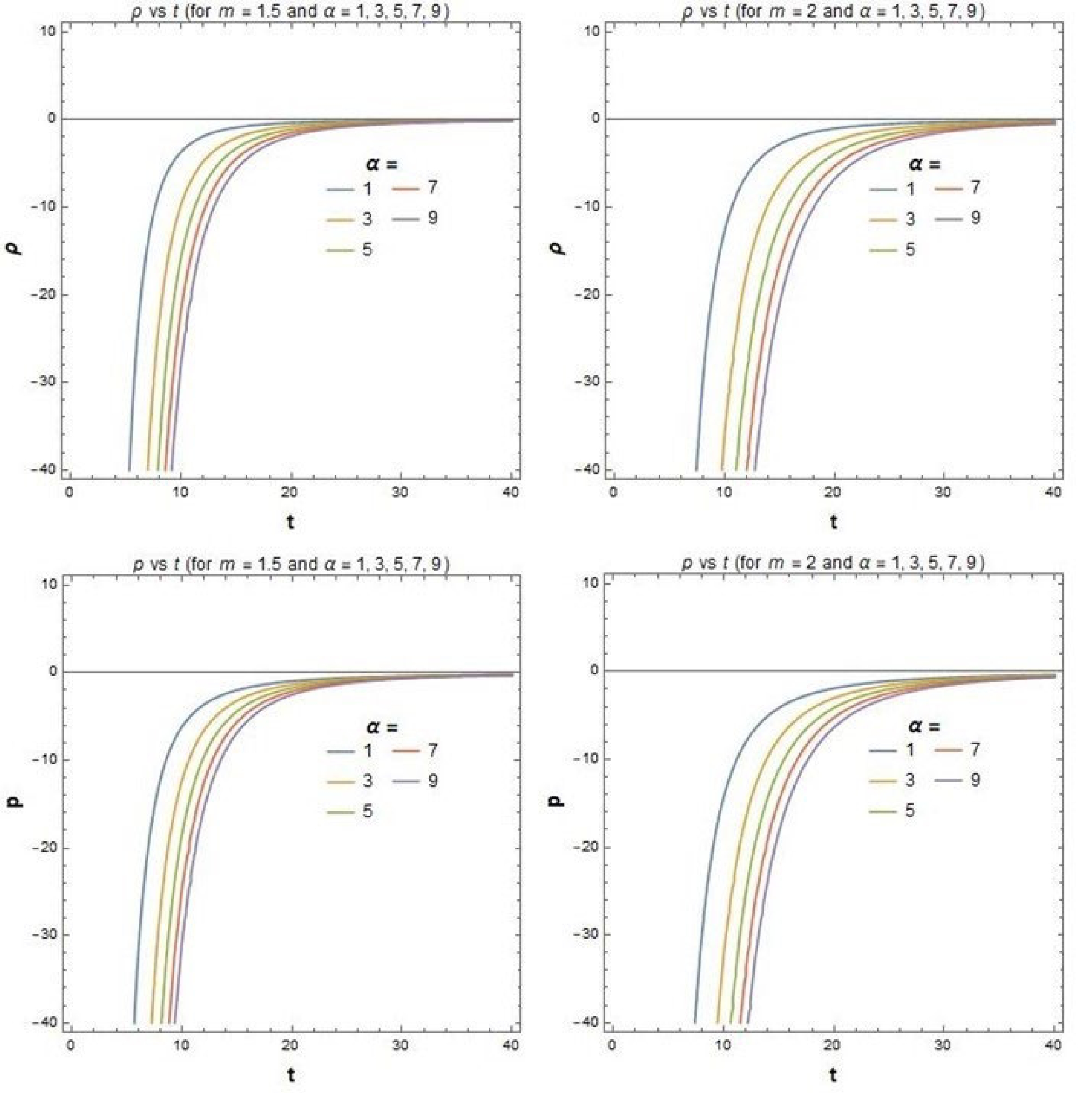
Figure 1. (color online) Variation of ρ and p with t for different values of m (
$ =1.5,2 $ ) and$ {\alpha} $ $ (=1,3,5,7,9) $ .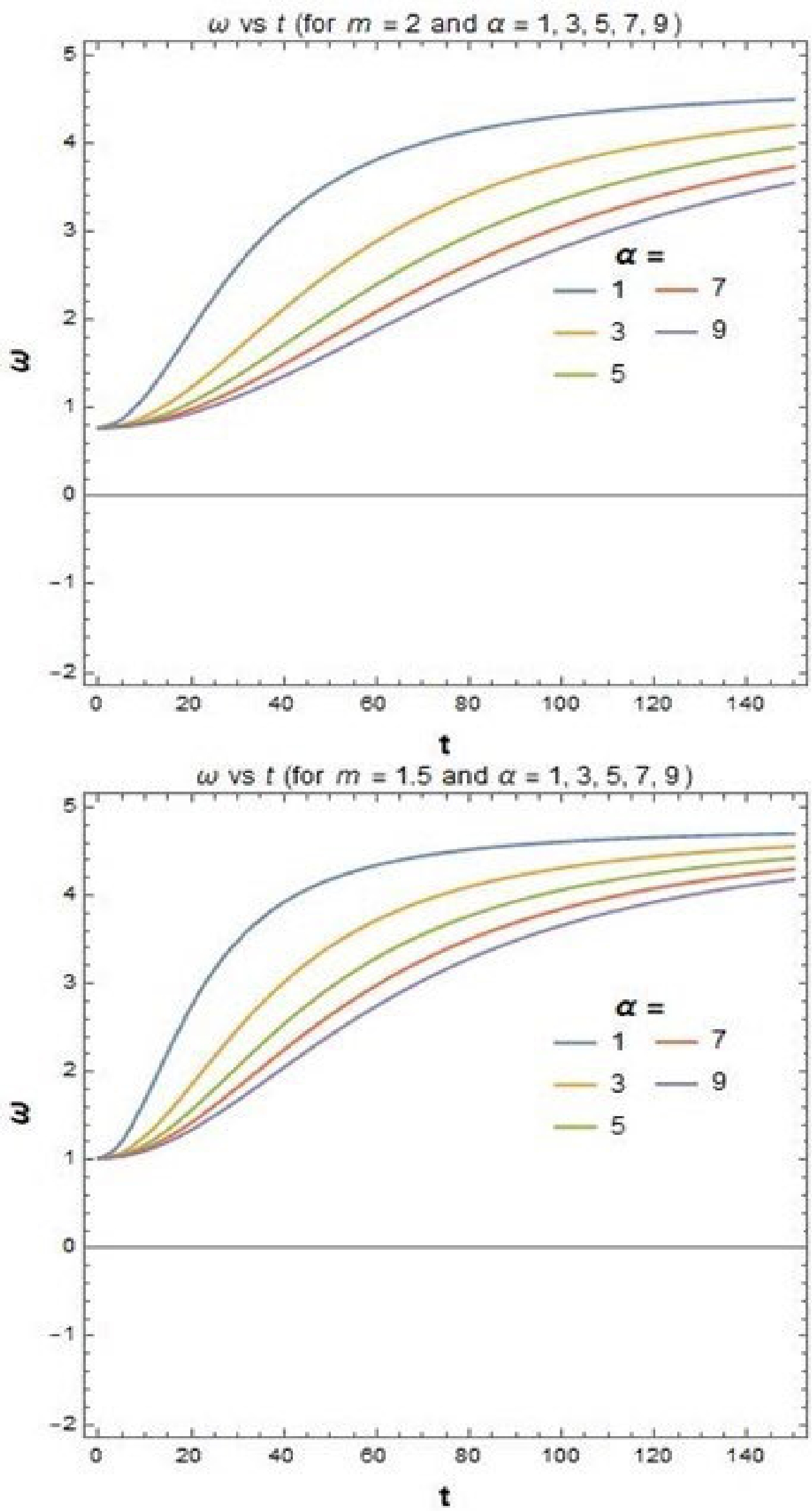
Figure 2. (color online) Variation of ω with t for different values of m (
$ =1.5,2 $ ) and$ {\alpha} $ $ (=1,3,5,7,9) $ .The negative values of α hav already been considered in [80] for
$ f(R,T) $ gravity. So, let's check the results of our model for a positive value of$ m(=2,3) $ and negative values of$ \alpha(=-0.9,-0.7,-0.5,-0.3,-0.1) $ . Figure 3 depicts the variation of ρ and p with time (t) for the above parameter values. Figure 4 shows the variation of the EOS parameter$ (\omega) $ with time$ (t) $ . From Fig. 3, it is evident that the value of ρ and p have the expected nature at a particular region of time. Simultaneously, Fig. 4 produces the anticipated value of ω, which is$ -1 $ for the dark energy epoch. We discuss the results more elaborately obtained in Figs. 3 and 4 in the following subsection.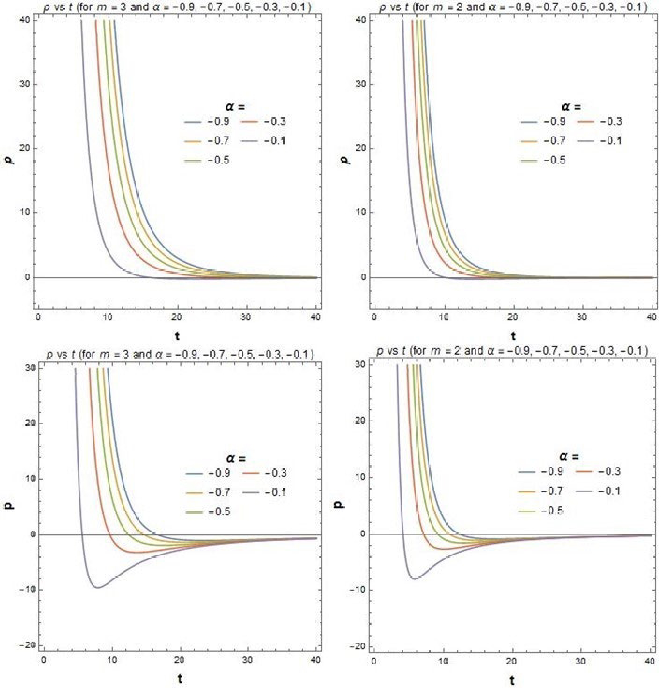
Figure 3. (color online) Variation of ρ and p with t for different values of m (
$ =3,2 $ ) and$ {\alpha}(=-0.9,-0.7,-0.5,-0.3,-0.1) $ .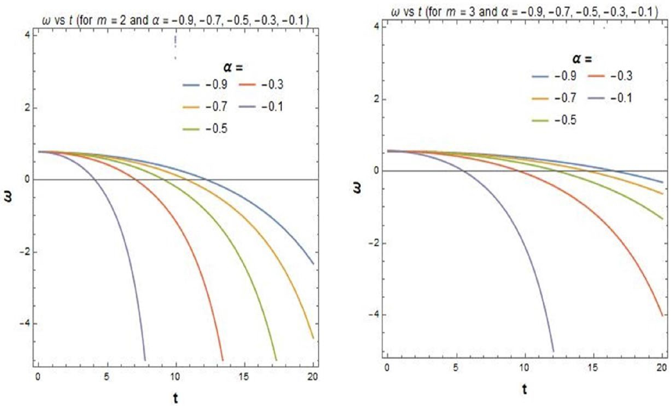
Figure 4. (color online) Variation of ω with t for different values of m (
$ =2, 3 $ ) and$ {\alpha} $ $ (=-0.1,-0.3,-0.5,-0.7,-0.9) $ . -
Before entering into this section, we would like to discuss two significant works, one was done by Tripathi et al. [81] and the other one was done by Moraes et al. [80]. In [81], they constrained the dark energy models for low redshifts and compared the data with the observations of Supernova Type Ia data, Baryon Acoustic Oscillation data, and Hubble parameter measurements. On the other hand, in [80], the authors studied various cosmological aspects with the help of the Starobinsky model in the framework of
$ f(R,T) $ gravity. They found the nature of material content of the universe, i.e. ρ and p in both decelerated and accelerated regimes of the universe.The variation of ρ and p with time obtained in Fig. 3 is quite similar with the variation obtained in [80], though our models differ from each other. Figure 3 shows that at early time (
$ t\rightarrow 0 $ ), the pressure was positive. But, after a certain value of time, it takes negative value, which may be correlated with the effect of the negative pressure fluid responsible for the accelerating universe. We have shown a table which depicts that for different choices of the positive m and the negative α, and we get a range of t (from Fig. 4) where the value of ω agrees with the observational data of Supernova Type Ia data, Baryon Acoustic Oscillation data, and Hubble parameter measurements (Observational data are taken from [81]). Furthermore, if we concentrate on the range of t that has been shown in Table 1 and match those values with Fig. 3, then can be observed that at those particular time regions, the value of p takes the negative sign, whereas the ρ is positive.m α t ω ( $ 3\sigma $ confidence)

Observation 2 $ -0.9 $ 

$ 14.96-15.5 $ 

$ -0.95\geq\omega\geq-1.13 $ 

SNIa+ BAO+ H(z) 3 $ 22.8-23.87 $ 

2 $ -0.7 $ 

$ 13.2-13.67 $ 

3 $ 20.1-21.05 $ 

2 $ -0.5 $ 

$ 11.16-11.55 $ 

3 $ 17.06-17.8 $ 

2 $ -0.3 $ 

$ 8.64-8.95 $ 

3 $ 13.22-13.78 $ 

2 $ -0.1 $ 

$ 4.98-5.16 $ 

3 $ 7.63-7.97 $ 

Table 1. Table for Observational Verification of the Model.
-
With the help of the modified field equation (27) for
$ f({\bar{R}},L(X)) $ theory, the emergent Einstein's equation (15) can be written as ($ {\kappa}=1 $ )$ {\bar{R}}_{\mu\nu}-\frac{1}{2}{\bar{G}}_{\mu\nu}{\bar{R}}=T_{\mu\nu}^{\rm eff}, $

(75) where
$ \begin{aligned}[b] T_{\mu\nu}^{\rm eff}=&\frac{1}{F}[\frac{1}{2}f_{L}{\bar{T}}_{\mu\nu}-\frac{1}{2}{\bar{R}} F{\bar{G}}_{\mu\nu}-({\bar{G}}_{\mu\nu}\bar{\square}-D_{\mu}D_{\nu})F\\&+\frac{1}{2}{\bar{G}}_{\mu\nu}(f-Lf_{L}(1+D_{{\alpha}}\phi D^{{\alpha}}\phi))\\&-\frac{1}{2}Lf_{L}D_{\mu}\phi D_{\nu}\phi(1+D_{{\alpha}}\phi D^{{\alpha}}\phi)] \\ =&\frac{1}{F}[\frac{1}{2}f_{L}{\bar{T}}_{\mu\nu}+\frac{1}{2}{\bar{G}}_{\mu\nu}(f-F{\bar{R}})-({\bar{G}}_{\mu\nu}\bar{\square}-D_{\mu}D_{\nu})F\\&-\frac{1}{2}Lf_{L}{\bar{G}}_{\mu\nu}(1+D_{\mu}\phi D^{\mu}\phi)^{2}], \end{aligned} $

(76) with
$ F=f_{{\bar{R}}}=\dfrac{{\partial} f({\bar{R}},L(X))}{{\partial} {\bar{R}}} $ .The trace of the effective energy momentum tensor (76) is
$ \begin{aligned}[b] T^{\rm eff}=&\frac{1}{F}[\frac{1}{2}f_{L}{\bar{T}} +2(f-F {\bar{R}})-3 \bar{\square} F-\\&2Lf_{L}(1+D_{\mu}\phi D^{\mu}\phi)^{2}]. \end{aligned} $

(77) Now, from Eq. (75), we have the emergent Ricci tensor in terms of the effective energy momentum tensor as
$ {\bar{R}}_{\mu\nu}=T_{\mu\nu}^{\rm eff}-\frac{1}{2}{\bar{G}}_{\mu\nu}T^{\rm eff}. $

(78) Let
$ \bar{u}^{\mu} $ be the tangent vector field to a congruence of time-like geodesics in the K-essence emergent space-time manifold endowed with the metric$ {\bar{G}}_{\mu\nu} $ ($ {\bar{G}}_{\mu\nu}\bar{u}^{\mu}\bar{u}^{\nu}=1 $ ), then the strong energy condition (SEC) (107) in$ f({\bar{R}},L(X)) $ modified gravity can be expressed as$ {\bar{R}}_{\mu\nu}\bar{u}^{\mu}\bar{u}^{\nu}=(T_{\mu\nu}^{\rm eff}\bar{u}^{\mu}\bar{u}^{\nu}-\frac{1}{2}T^{\rm eff})\geq 0. $

(79) On the other hand, if we consider
$ \bar{k}^{\mu} $ be the tangent vector along the null geodesic congruence ($ {\bar{G}}_{\mu\nu}\bar{k}^{\mu}\bar{k}^{\nu}=0 $ ), then the null energy condition (NEC) (109) in$ f({\bar{R}},L(X)) $ gravity is$ {\bar{R}}_{\mu\nu}\bar{k}^{\mu}\bar{k}^{\nu}=T_{\mu\nu}^{\rm eff}\bar{k}^{\mu}\bar{k}^{\nu}\geq 0. $

(80) So, considering an additional condition [19]
$ \dfrac{f_{L}({\bar{R}},L)}{f_{{\bar{R}}}({\bar{R}},L)}>0 $ , and the K-essence scalar field to be homogeneous, i.e.,$ \phi(x^{i},t)\equiv \phi(t) $ , and using the perfect fluid energy momentum tensor (44), we have the SEC and NEC in the$ f({\bar{R}},L(X)) $ gravity are$ \begin{aligned}[b] SEC:&\; \bar{\rho}+3\bar{p}-\frac{2}{f_{L}}(f-F{\bar{R}})+2L(1+\dot\phi^{2})^{2}\\&+\frac{6}{f_{L}(1-\dot\phi^{2})}[\ddot{F}(1-\frac{2}{3}\dot\phi^{2})+H\dot{F}(1-\dot\phi^{2}+\frac{2}{3}\dot\phi^{4})]\geq 0, \end{aligned} $

(81) $ NEC: \bar{\rho}+\bar{p}+\frac{2}{f_{L}}(\ddot{F}-H\dot{F}\dot\phi^{2})\geq 0, $

(82) where
$ \bar{\rho}=\rho(1+\dot\phi^{2}) $ and$ \bar{p}=p(1+\dot\phi^{2}) $ .To evaluate the effective density,
$\bar{\rho}^{\rm eff}$ , and effective pressure,$\bar{p}^{\rm eff}$ , in the K-essence emergent$ f({\bar{R}},L(X)) $ gravity, we consider the two following equations$ T_{\mu\nu}^{\rm eff}\bar{u}^{\mu}\bar{u}^{\nu}-\frac{1}{2}{\bar{G}}_{\mu\nu}T^{\rm eff}\bar{u}^{\mu}\bar{u}^{\nu}=\bar{\rho}^{\rm eff}+3\bar{p}^{\rm eff}, $

(83) and
$ T_{\mu\nu}^{\rm eff}\bar{k}^{\mu}\bar{k}^{\nu}=\bar{\rho}^{\rm eff}+\bar{p}^{\rm eff}. $

(84) Solving these Eqs. (49) and (50), we get
$ \begin{aligned}[b] \bar{\rho}^{\rm eff}=&\bar{\rho}+\frac{1}{f_{L}}(f-F{\bar{R}})-\frac{6}{f_{L}(1-\dot\phi^{2})}[\frac{1}{3}\ddot{F}\dot\phi^{2}\\&+H\dot{F}(1-\frac{1}{3}\dot\phi^{4})]-L(1+\dot\phi^{2})^{2}, \end{aligned} $

(85) $ \begin{aligned}[b] \bar{p}^{\rm eff}=&\bar{p}-\frac{1}{f_{L}}(f-F{\bar{R}})+\frac{3}{f_{L}(1-\dot\phi^{2})}[\frac{1}{3}\ddot{F}(2-\dot\phi^{2})\\&+H\dot{F}(1-\frac{2}{3}\dot\phi^{2}+\frac{1}{3}\dot\phi^{4})]+L(1+\dot\phi^{2})^{2}. \end{aligned} $

(86) From the above Eqs. (85) and (86), we have WEC and DEC, respectively, for the K-essence emergent
$ f({\bar{R}},L(X)) $ gravity as$ \begin{aligned}[b] WEC:& \bar{\rho}+\frac{1}{f_{L}}(f-F{\bar{R}})-\frac{6}{f_{L}(1-\dot\phi^{2})}\Big[\frac{1}{3}\ddot{F}\dot\phi^{2}\\&+H\dot{F}(1-\frac{1}{3}\dot\phi^{4})\Big]-L(1+\dot\phi^{2})^{2}\geq 0, \end{aligned} $

(87) $ \begin{aligned}[b] DEC:&\bar{\rho}-\bar{p}+\frac{2}{f_{L}}(f-F{\bar{R}})-\frac{2}{f_{L}(1-\dot\phi^{2})}[\ddot{F}(1+\frac{1}{2}\dot\phi^{2})\\&+3H\dot{F}(\frac{3}{2}-\frac{1}{3}\dot\phi^{2}-\frac{1}{6}\dot\phi^{4})]-2L(1+\dot\phi^{2})^{2}\geq 0. \end{aligned} $

(88) These energy conditions (81), (82), (87), and (88) of the K-essence emergent
$ f({\bar{R}},L(X)) $ gravity are different from the usual$ f(R,L_{m}) $ -gravity (111) and$ f(R) $ -gravity (110) in the presence of the K-essence scalar field, ϕ. Also, note that if we consider$ f({\bar{R}},L(X))\equiv R $ and$ {\bar{G}}_{\mu\nu}\equiv g_{\mu\nu} $ , then we can get back to the usual energy conditions of GR, i.e.,$ SEC:\; \rho+3p\geq 0 $ ;$ NEC:\; \rho+p\geq 0 $ ; and$ WEC:\; \rho\geq 0 $ and$ DEC:\; \rho\geq |p| $ .One may notice that we briefly have discussed the energy conditions of
$ f(R) $ and$ f(R,L_m) $ gravity in the Appendix. -
The inequalities of the energy conditions (81), (82), (87), and (88) can also be expressed in terms of the deceleration (q), jerk (j), and snap (s) parameters such that the Ricci scalar and its derivatives for a spatially flat K-essence emergent FLRW geometry (37) are
$ {\bar{R}}=\frac{6}{1-\dot\phi^{2}}\left[\dot H +H^{2}(2-\dot\phi^{2})\right]=\frac{6H^{2}}{1-\dot\phi^{2}}\left[1-q-\dot\phi^{2}\right], $

(89) $ \begin{aligned}[b] \dot{{\bar{R}}}=&\frac{6}{1-\dot\phi^{2}}\left[\ddot{H}+4H\dot{H}(1-\dot\phi^{2})-2H^{3}\dot\phi^{2}\right] \\=&\frac{6H^{3}}{1-\dot\phi^{2}}\left[(j-q-2)+2\dot\phi^{2}(1-2q)\right], \end{aligned} $

(90) $ \begin{aligned}[b] \ddot{{\bar{R}}}=&\frac{6}{1-\dot\phi^{2}}[(\dot{\ddot{H}}+4\dot{H}^{2}+4H\ddot{H})\\&-2\dot\phi^{2}(2\dot{H}^{2}+3H\ddot{H}-2H^{4}+3H^{2}\dot{H}] \\=&\frac{6H^{4}}{1-\dot\phi^{2}}[(s+q^{2}+8q+6)-2\dot\phi^{2}(3+3j+10q+2q^{2})], \end{aligned} $

(91) $ q=-\frac{1}{H^{2}}\frac{\ddot{a}}{a}\; ;\; j=\frac{1}{H^{3}}\frac{\dot{\ddot{a}}}{a}\; ;\; s=\frac{1}{H^{4}}\frac{\ddot{\ddot{a}}}{a}. $

(92) Now, from Eq. (51), we evaluate the values of
$ \dot{F} $ and$ \ddot{F} $ (using Eq. (38)) in terms of$q,\; j,\; {\rm{and}} \; s$ as$ \begin{aligned}[b] \dot{F}=&\frac{6H^{3}}{1-\dot\phi^{2}}F_{{\bar{R}}}[(j-q-2)+2\dot\phi^{2}(1-2q)]\\&-HF_{L}L_{XX}\dot\phi^{2}(1-\dot\phi^{2}), \end{aligned}$

(93) $ \begin{aligned}[b] \ddot{F}=&\frac{6H^{4}}{1-\dot\phi^{2}}F_{{\bar{R}}}[(s+q^{2}+8q+6)-2\dot\phi^{2}(3+3j+10q+2q^{2})] \\&+\frac{36H^{6}}{(1-\dot\phi^{2})^{2}}F_{{\bar{R}}{\bar{R}}}[(j-q-2)+2\dot\phi^{2}(1-2q)]^{2}\\&+H\dot\phi^{4}(1-\dot\phi^{2})^{2}\left(F_{LL}L_{X}^{2}+F_{L}L_{XX}\right)\\&-F_{L}L_{X}\dot\phi^{2}(1-\dot\phi^{2})[\dot{H}-2H^{2}(1-2\dot\phi^{2})].\; \; \end{aligned} $

(94) Therefore, putting these values of
$ \dot{F} $ and$ \ddot{F} $ into the energy conditions (81), (82), (87), and (88), we have the energy conditions in terms of q, j, and s. We can easily check that these energy conditions in terms of q, j, and s are also different from the$ f(R,L_{m}) $ -gravity [19] in the presence of the K-essence scalar field, ϕ. -
Considering the Starobinsky Model, i.e., Eq. (54), we obtain the following results as
$ f_{L}=1 $ ,$ F=1+2\alpha{\bar{R}} $ ,$ \dot{F}=2\alpha\dot{{\bar{R}}} $ , and$ \ddot{F}=2\alpha\ddot{{\bar{R}}} $ .Using these results we get the energy conditions from (81), (82), (87), and (88) as follows:
$ \begin{aligned}[b] SEC :\;& \bar{\rho}+3\bar{p}+2\left[\alpha{\bar{R}}^{2}+L\dot{\phi}^2(2+\dot{\phi}^2)\right]\\&+\frac{12\alpha\ddot{{\bar{R}}}}{1-\dot{\phi}^2}\left(1-\frac{2}{3}\dot{\phi}^2\right) +\frac{12\alpha H\dot{{\bar{R}}}}{1-\dot{\phi}^2}\left(1-\dot{\phi}^2+\frac{2}{3}\dot{\phi}^4\right)\geq 0 \end{aligned} $

(95) $ NEC :\; \bar{\rho}+\bar{p}+4\alpha\left(\ddot{{\bar{R}}}-H\dot{{\bar{R}}}\dot{\phi^2}\right)\geq 0 $

(96) $ \begin{aligned}[b] WEC :\;&\bar{\rho}-\alpha{\bar{R}}^{2}-\frac{4\alpha}{1-\dot{\phi}^2}\left[\ddot{{\bar{R}}}\dot{\phi}^2-3\dot{{\bar{R}}}(1-\frac{1}{3}\dot{\phi}^4)\right]\\&-L\dot{\phi}^2(2-\dot{\phi}^2)\geq 0 \end{aligned} $

(97) $ \begin{aligned}[b] DEC :\;&\bar{\rho}-\bar{p}-2\alpha{\bar{R}}^{2}-\frac{4\alpha}{1-\dot{\phi}^2}\Bigg[\ddot{{\bar{R}}}(1-\frac{1}{2}\dot{\phi}^2)\\&-3H\dot{{\bar{R}}}\left(\frac{3}{2}-\frac{1}{3}\dot{\phi}^2-\frac{1}{6}\dot{\phi}^4\right)\Bigg]-2L\dot{\phi}^2(2+\dot{\phi}^2)\geq 0\; \; \end{aligned} $

(98) Again, if we put the values of
$ {\bar{R}} $ ,$ \dot{{\bar{R}}} $ , and$ \ddot{{\bar{R}}} $ from (89), (90), and (91) into the above equations (95), (96), (97), and (98), we easily reconstruct the energy conditions in terms of the deceleration (q), jerk (j), and snap (s) parameters. -
In this work, we present a new type of modified theory, viz.
$ f({\bar{R}}, L(X)) $ -gravity, with a general formalism in the context of dark energy (using K-essence emergent geometry) where$ {\bar{R}} $ is the Ricci scalar of this geometry,$ L(X) $ is the DBI type non-canonical Lagrangian with$ X={1\over 2}g^{\mu\nu}\nabla_{\mu}\phi\nabla_{\nu}\phi $ , and ϕ is the K-essence scalar field. The K-essence emergent metric,$ {\bar{G}}_{\mu\nu} $ , is not conformally equivalent to the gravitational metric,$ g_{\mu\nu} $ . This new type of modified theory is a general mixing between$ f(R) $ gravity and K-essence emergent gravity based on the DBI model.Let us discuss some salient features of the present study which are as follows:
(1) It is to be noted that the modified field equation (27) is different from the usual
$ f(R) $ and$ f(R,L_{m}) $ gravities. If we consider$ f({\bar{R}},L(X))\equiv R $ and$ {\bar{G}}_{\mu\nu}\equiv g_{\mu\nu} $ , then we can easily get back to the standard Einstein field equation. The effective functional relation for the requirement of the conservation of the energy-momentum tensor is also different from$ f(R,L_{m}) $ -gravity. We derive the modified Friedmann equations for the$ f({\bar{R}},L(X)) $ -gravity considering the background gravitational metric as flat FLRW and the K-essence scalar field, ϕ, being simply a function of time only, which are quite different from the Friedmann equations of the standard$ f(R) $ gravity.(2) For the particular choice (viz. Starobinksy-type), Eq. (54) of
$ f({\bar{R}},L) $ and from the requirement of the energy-momentum conservation (32), the kinetic energy of the K-essence scalar field is a constant. This value of$ \dot\phi^{2} $ ($ =0.888 $ ) is less than unity, which is comparable with the range of$ \dot\phi^{2} $ . It is also noted that the K-essence theory can be used to investigate the effects of the presence of dark energy on cosmological scenarios. In this context, if we consider$ \dot\phi^{2} $ to be dark energy density in unit of critical density as [40–42], then the value of dark energy density, i.e.,$ \dot\phi^{2}=\frac{8}{9}=0.888 $ , indicates that the present universe is dark-energy dominated.It is well known that the present observational value [86, 87] of dark energy density is approximately
$ 0.75 $ . Therefore, we note that in the context of the dark energy regime, our result is in good agreement with observational data. Nowadays, people believe that dark energy is one of the reasons for the accelerating universe. So, our value of dark energy density may indicate that the universe is more accelerating. From Figs. 3 and 4, we also observe that our model is observationally verified for certain values of parameters. According to Fig. 3, the negativity of pressure can be achieved after a certain value of time, which may be responsible for the accelerating universe. The variation of EOS ($ {\omega} $ ) with time (t) in Fig. 4 shows that$ {\omega} $ approaches negative values, which corresponds to observational results [81] of the present universe.Also, we would like to put here the following two special aspects which emerge from the present investigation: (i) This model can open up an alternative window to explore the current cosmic acceleration without a stringent condition of invoking an exotic component as the dark energy. In other words, this theory seems interesting from a purely gravitational theory standpoint, rather than the cosmological context of dark energy whose very existence is still an issue of doubt [88] according to the latest analysis of data from the Planck consortium [86, 87]. However, the arbitrariness in the choice of different functional forms of
$ f({\bar{R}},L(X)) $ based on a DBI Lagrangian gives rise to the problem of how to constrain the many possible$ f({\bar{R}},L(X)) $ gravity theories on physical grounds. In this context, we have shed some light on this issue by discussing some constraints on general$ f({\bar{R}},L(X)) $ gravity from the so-called energy conditions. (ii) Also, we have derived the null, strong, weak, and dominant energy conditions in the framework of$ f({\bar{R}},L(X)) $ gravity from the Raychaudhuri equations. These energy conditions are different from the usual$ f(R,L_{m}) $ and$ f(R) $ theories. With the help of the specific form of$ f({\bar{R}},L(X)) $ , we also have derived these energy conditions in$ f({\bar{R}},L(X)) $ -gravity.However, we intend to report on this interesting theory in the near future encompassing the multifarious aspects of cosmology.
-
All of the authors would like to thank the referee for illuminating suggestions to improve the manuscript.
-
Let us consider here the well known
$ f(R) $ and$ f(R,L_{m}) $ gravity, where R is the Ricci scalar with respect to the gravitational metric,$ g_{\mu\nu} $ , and$ L_{m} $ is the matter Lagrangian. The total action for the$ f(R) $ gravity is [6, 7]$ S=\frac{1}{2\kappa}\int {\rm d}^{4}x\sqrt{-g}f(R)+S_{M}(g_{\mu\nu},\psi), \tag{A1}$

where
$ S_{M} $ is the matter term, ψ denotes the matter fields,$ {\kappa}=8\pi G $ , G is the gravitational constant, g is the determinant of the gravitational metric, and$ R\; (=g^{\mu\nu}R_{\mu\nu}) $ is the Ricci scalar.Varying with respect to the gravitational metric, we achieve the modified field equation as
$ f'(R)R_{\mu\nu}-\frac{1}{2}f(R)g_{\mu\nu}-[\nabla_{\mu}\nabla_{\nu}-g_{\mu\nu}\Box]f'(R)={\kappa} T_{\mu\nu},\tag{A2}$

with
$ T_{\mu\nu}= \frac{-2}{\sqrt{-g}}\frac{\delta S_{M}}{\delta g^{\mu\nu}}, \tag{A3} $

where
$ f'(R)=\dfrac{{\partial} f(R)}{{\partial} R} $ ,$ \nabla_{\mu} $ is covariant derivative with respect to the gravitational metric, and$ \square\equiv \nabla^{\mu}\nabla_{\mu} $ .On the other hand, the action for the
$ f(R,L_{m}) $ gravity is [18, 19]$ S=\frac{1}{2\kappa}\int {\rm d}^{4}x\sqrt{-g}f(R,L_{m}), \tag{A4} $

where
$ f(R,L_{m}) $ is an arbitrary function of the Ricci scalar R, and the Lagrangian density corresponding to matter,$ L_{m} $ . The energy-momentum tensor is$ T_{\mu\nu}= \frac{-2}{\sqrt{-g}}\frac{\delta (\sqrt{-g}L_{m})}{\delta g^{\mu\nu}}=-2\frac{{\partial} L_{m}}{{\partial} g^{\mu\nu}}+g_{\mu\nu}L_{m},\; \; \tag{A5} $

where the Lagrangian density,
$ L_{m} $ , is only matter dependent on the metric tensor components,$ g_{\mu\nu} $ .The modified field equations of the
$ f(R,L_{m}) $ -gravity model is$ \begin{aligned}[b] &f_{R}(R,L_{m})R_{\mu\nu}+(g_{\mu\nu}\square-\nabla_{\mu}\nabla_{\nu})f_{R}(R,L_{m})\\&-\frac{1}{2}[f(R,L_{m})-L_{m}f_{L_{m}}(R,L_{m})]g_{\mu\nu} \\=& \frac{1}{2}f_{L_{m}}(R,L_{m})T_{\mu\nu},\; \; \; \end{aligned}\tag{A6} $

where
$ f_{R}(R,L_{m})={\partial} f(R,L_{m})/{\partial} R $ and$ f_{L_{m}}(R,L_{m})= {\partial} f(R,L_{m})/{\partial} L_{m} $ . However, if$ f(R,L_{m})=R/2+L_{m} $ , then the above Eq. (A6) reduces to the usual field equation$ R_{\mu\nu}-(1/2)g_{\mu\nu}R={\kappa} T_{\mu\nu} $ . -
Following most of the techniques of [10–14, 19, 73], we will derive the energy conditions for modified (
$ f(R) $ ,$ f(R,L_{m}) $ , etc.) gravities. From these theories we can approach the Null Energy Condition (NEC) and Strong Energy Condition (SEC) in the context of GR. The origin of these energy conditions comes from the Raychaudhuri equations. Let$ u^{\mu} $ be the tangent vector field to a congruence of time-like geodesics in a space-time manifold endowed with a metric,$ g_{\mu\nu} $ . Therefore, the Raychaudhuri equation [89–94] is$ \frac{{\rm d}{\theta}}{{\rm d}\tau}=-\frac{1}{3}{\theta}^{2}-{\sigma}_{\mu\nu}{\sigma}^{\mu\nu}+{\omega}_{\mu\nu}{\omega}^{\mu\nu}-R_{\mu\nu}u^{\mu}u^{\nu}, \tag{B1} $

where
$ R_{\mu\nu} $ is the Ricci tensor corresponding to the metric$ g_{\mu\nu} $ , and$ {\theta} $ ,$ {\sigma}_{\mu\nu} $ , and$ {\omega}_{\mu\nu} $ are the expansion, shear, and rotation associated with the congruence, respectively. While in the case of a congruence of null geodesics defined by the vector field,$ k^{\mu} $ , the Raychaudhuri equation [92] is given by$ \frac{{\rm d}{\theta}}{{\rm d}\tau}=-\frac{1}{2}{\theta}^{2}-{\sigma}_{\mu\nu}{\sigma}^{\mu\nu}+{\omega}_{\mu\nu}{\omega}^{\mu\nu}-R_{\mu\nu}k^{\mu}k^{\nu}. \tag{B2} $

These equations are purely based on geometric statements, and as such it makes no reference to any gravitational field equations. In other words, the Raychaudhuri equation can be thought of as geometrical identities, which do not depend on any gravitational theory. These equations provide the evolution of the expansion of a geodesic congruence. However, since the GR field equations relate
$ R_{\mu\nu} $ to the energy-momentum tensor,$ T_{\mu\nu} $ , the combination of Einstein and Raychaudhuri equations can be used to restrict energy-momentum tensors on physical grounds. Indeed, the shear is a "spatial" tensor given by$ {\sigma}^{2}\equiv {\sigma}_{\mu\nu}{\sigma}^{\mu\nu}\geq 0 $ .Thus, it is clear from the Raychaudhuri equation that for any hypersurface orthogonal congruences (
$ {\omega}_{\mu\nu}\equiv 0 $ ), the condition for attractive gravity (convergence of timelike geodesics or geodesic focusing) reduces to ($ R_{\mu\nu}u^{\mu}u^{\nu}\geq 0 $ ), which by virtue of Einstein’s equation implies$ R_{\mu\nu}u^{\mu}u^{\nu}=(T_{\mu\nu}-\frac{T}{2}g_{\mu\nu})u^{\mu}u^{\nu}\geq 0, \tag{B3} $

where T is the trace of the energy momentum tensor,
$ T_{\mu\nu} $ ($ {\kappa}=1 $ ). Here, Eq. (B3) is nothing but the SEC stated in a coordinate-invariant way in terms of$ T_{\mu\nu} $ and vector fields of fixed (time-like) character. Thus, in the context of GR, the SEC ensures the fact that the gravity is attractive. In particular, for a perfect fluid of density, ρ, and pressure, p,$ T_{\mu\nu}=(\rho +p)u_{\mu}u_{\nu}-pg_{\mu\nu} \tag{B4} $

and the restriction given by Eq. (B3) takes the familiar form for the SEC, i.e.,
$ \rho +3p \geq 0 $ .On the other hand, the condition for the convergence (geodesic focusing) of hypersurface orthogonal (
$ {\omega}_{\mu\nu}\equiv 0 $ ) congruences of null geodesics along with Einstein’s equation implies$ R_{\mu\nu}k^{\mu}k^{\nu}=T_{\mu\nu}k^{\mu}k^{\nu} \geq 0 \tag{B5} $

which is the condition for NEC written in a coordinate-invariant way.
Thus, in GR the NEC ultimately encodes the null geodesic focusing due to the gravitational attraction. For the energy-momentum tensor of a perfect fluid (B4), the above condition (B5) reduces to the well-known form of the NEC, i.e.,
$ \rho +p\geq 0 $ .The Weak Energy Condition (WEC) states that
$ T_{\mu\nu}u^{\mu}u^{\nu}\geq 0 $ for all time-like vectors,$ u^{\mu} $ , or equivalently for perfect fluid it is$ \rho>0 $ and$ \rho +p>0 $ . The Dominant Energy Condition (DEC) includes the WEC, as well as the additional requirement that$ T_{\mu\nu}u^{\mu} $ is a non space-like vector, i.e.,$ T_{\mu\nu}T^{\nu}_{{\lambda}}u^{\mu}u^{{\lambda}}\leq 0 $ . For a perfect fluid, these conditions, together, are equivalent to the simple requirement that$ \rho\geq |p| $ , the energy density must be non-negative, and greater than or equal to the magnitude of the pressure.In
$ f(R) $ -gravity [10, 11], the energy conditions for perfect fluid are given by$ \begin{aligned}[b] &SEC:\; \; \rho +3p-f+Rf'+3(\ddot{R}+\dot{R}H)f"+3\dot{R}^{2}f"'\geq 0,\\ &NEC:\; \; \rho +p+(\ddot{R}-\dot{R}H)f"+\dot{R}^{2}f"'\geq 0,\\ &WEC:\; \; \rho+\frac{1}{2}(f-Rf')-3\dot{R}Hf"\geq 0,\\ \end{aligned} $

$ \begin{aligned}[b] &DEC:\; \rho-p+f-Rf'-(\ddot{R}+5\dot{R}H)f"-\dot{R}^{2}f"'\geq 0, \end{aligned}\tag{B6} $

where
$ f'=\dfrac{{\partial} f(R)}{{\partial} R} $ .In
$ f(R,L_{m}) $ -gravity [19], the energy conditions are$ \begin{aligned}[b] &SEC: \rho +3p-\frac{2}{f_{L_{m}}}[f-Rf']+\frac{6}{f_{L_{m}}}[\dot{R}^{2}f"' +\ddot{R}f" \\&+H\dot{R}f"]-2L_{m}\geq 0.\\ &NEC: \rho +p+\frac{2}{f_{L_{m}}}[\dot{R}^{2}f"' +\ddot{R}f" ]\geq 0,\\& WEC: \rho+\frac{1}{f_{L_{m}}}[f-Rf']-\frac{6}{f_{L_{m}}}H\dot{R}f"+L_{m}\geq 0,\\ &DEC: \rho-p+\frac{2}{f_{L_{m}}}[f-Rf']-\frac{2}{f_{L_{m}}}\Big[\dot{R}^{2}f"' +\ddot{R}f"+6H\dot{R}f"\Big]\\&+2L_{m}\geq 0, \end{aligned}\tag{B7} $

where
$ f'=\dfrac{{\partial} f(R,L_{m})}{{\partial} R} $ .
${ \boldsymbol f(\bar{\boldsymbol R}, \boldsymbol L(\boldsymbol X))} $ -gravity in the context of dark energy with power law expansion and energy conditions
- Received Date: 2022-08-20
- Available Online: 2023-02-15
Abstract: The objective of this work is to generate a general formalism of


 DownLoad: