Large signal of h → µτ within the constraints of e_i → e_jγ decays in the 3-3-1 model with neutral leptons

Experimental data have confirmed the existence of flavor neutrino oscillations through the precise values of their mixing angles and their mass squared deviation [1]. This is an important assumption about lepton-flavor-violating (LFV) decays. There are two types of LFV decays that have received considerable attention, the lepton-flavor-violating decays of charged leptons (cLFV) and the lepton-flavor-violating decays of standard model- like Higgs bosons (LFVHDs). These LFV decays are considered in both theory and experiment. On the experimental side, the cLFV are constrained by upper bounds, as given in Ref. [2],

These are currently the most stringent experimental limits for cLFV. It should be recalled that in addition to the cLFV limits given at Eq. (1), we are interested in two other decay processes: $\mu \rightarrow 3e$ and $\mu \rightarrow e$ conversion in nuclei. Moreover, we place experimental limits on these decay processes, ${\rm Br}(\mu \rightarrow 3e)<10^{-12}$ from Ref. [3] and ${\rm CR}(\mu^-Ti \rightarrow e^- Ti)<6.1\times 10^{-13}$ from Ref. [4], respectively. These limits are considered looser than that originating from ${\rm Br}(\mu \rightarrow e\gamma)$. Therefore, the limit of ${\rm Br}(\mu \rightarrow e\gamma)$ can be used to find parameter space regions for the relevant process. Charged lepton flavor violation is considered a specific expression of the new physics we are searching for. A hypothesis of its contribution to the decays of heavy particles, such as Z bosons, Higgs bosons, and top quarks, is discussed in detail in Ref. [5].

For the LFVHDs, the experimental limits are given as in Refs. [6–10],

Then, there is an adjustment of ${\rm Br}(h \rightarrow \mu e) < 6.1 \times 10^{-5}$ according to the update in Ref. [11].

On the theoretical side, although LFV processes can generally receive tree and/or loop contributions, the LFV processes we study in this paper originate only from loop diagrams. We therefore consider both the fermion and boson contributions. The fermions mentioned here include ordinary charged leptons, exotic leptons, and neutrinos; however, ordinary charged leptons are assumed to be unmixed so that their contribution can be determined relatively simply. The complex part arises from neutrinos and exotic leptons with different mixing mechanisms. With active neutrinos, we can solve their masses and oscillations using seesaw mechanisms [12–18] or otherwise [19–22], and with exotic leptons, we make different assumptions for large LFV effects, as given in Refs. [19, 20, 23]. For the contribution of bosons, we consider both the charged gauge bosons and charged Higgs. The main contribution of the gauge bosons originates from new charged bosons, which are outside the standard model (SM), because the contribution of the W-boson is strongly suppressed by the GIM mechanism. The contributions of charged Higgs are varied and depend heavily on the energy scales of the accelerators.

It should be emphasized that LFV sources can mainly be found in models beyond the SM (BSM), and the parameter space domains predicted from BSM for the large signal of the LFVHDs, which we are interest in, are limited directly from both experimental data and theory of cLFV [24, 25]. Some published results show that ${\rm Br}(h_1^0\rightarrow \mu\tau)$ can reach values of ${\cal{O}}(10 ^ {-4})$ in supersymmetric and non-supersymmetric models [26–28]. In addition to the correction from the loop, other methods are also suggested in literature for large $h \rightarrow \mu \tau$ signals. For example, by using the type-I seesaw mechanism and an effective dimension-six operator, it is possible to accommodate the CMS $h \rightarrow \mu \tau$ signal with a branching ratio of the order of $10^{-2}$ [29]. In fact, the main contributions to ${\rm Br}(h_1^0\rightarrow \mu\tau)$ originate from new heavy particles BSM. If these contributions are minor or destructive, ${\rm Br}(h_1^0\rightarrow \mu\tau)$ in a model is only approximately ${\cal{O}}(10 ^ {-9})$ [12].

Recently, 3-3-1 models with multiple sources of LFV couplings have been used to investigate LFV decays [30–39]. However, these models can only give small LFV signals, or the cLFV and LFVHDs can achieve relatively large signals but in different regions of parameter space [20, 40–42]. Detailed calculations of the cLFV are given in Ref. [19] without mentioning the LFVHDs, whereas a 3-3-1 model mentioned in Ref. [40] only examines the LFVHDs. Several other versions of 3-3-1 models have used the inverse seesaw mechanism to study LFV decays. In this manner, it is necessary to introduce new particles that are singlets of the gauge group, leading to an increase in the number of particles and free parameters in these models [17]. The 3-3-1 model with neutral leptons can reduce the number of free parameters because without heavy particles that are singlets of the gauge group, the LFV source originates from the usual mixing of neutrinos and neutral leptons. This is a good model for studying both the cLFV and LFVHDs. Besides LFV decays, 3-3-1 models can also give large signals of other SM-like Higgs boson decays, such as $h^0_1\rightarrow \gamma \gamma$ and $h^0_1\rightarrow Z \gamma$ [43, 44].

In this study, we consider a 3-3-1 model to find regions of parameter space that satisfy the experimental limits of the cLFV. In these regions, we predict the existence of a large signal of the $h^0_1\rightarrow \mu \tau$ decay. Combined with the signal of $h^0_1\rightarrow Z \gamma$, as given in Ref. [43], we expect to have parameter space regions for large signals of both $h^0_1\rightarrow \mu \tau$ and $h^0_1\rightarrow Z \gamma$ decays.

This paper is organized as follows: In the next section, we review the model and give the mass spectra of gauge and Higgs bosons. We then show the mass spectra of all leptons in Section III. In Section IV, we calculate the Feynman rules and analytic formulas for the cLFV and LFVHDs. The numerical results are discussed in Section V, and conclusions are presented in Section VI. Finally, we provide Appendix A, B, C, and D to calculate and exclude divergence in the amplitude of the LFVHDs.

The 3-3-1 model with neutral leptons is a specific class of general 3-3-1 models (331β) that obey the gauge symmetry group $S U(3)_C\otimes S U(3)_L\otimes U(1)_X$ and the parameter $\beta=-\dfrac{1}{\sqrt{3}}$. The parameter β is a basis for defining the form of the electric charge operator in this model, $Q=T_3+\beta T_8+X$, where $T_{3,8}$ are diagonal $S U(3)_L$ generators. The model under consideration is developed based on the following highlights: i) Active neutrinos have no right-handed components; hence, they have only Majorana masses, which are generated from effective dimension-five operators, and there is no mixing among active neutrinos and exotic leptons [45]. ii) Exotic leptons are always assumed to have large mixing for the appearance of the LFV effect [40]. iii) There are two neutral Higgs that are identified with the corresponding ones of the two-Higgs-doublet model (THDM), with the expectation of having both large signals of the $h_1^0\rightarrow \mu\tau$ and $h_1^0\rightarrow Z\gamma$ decays. Thus, we call this model 331NL for short.

The leptons in the 331NL model are accommodated in triplet and singlet representations as follows:

where $a=1,2,3$ represents the family index for the usual three generations of leptons, and the numbers in the parentheses are the respective representations of the $S U(3)_C$, $S U(3)_L$, and $U(1)_X$ gauge groups. We use the primes to denote fermions in the flavor basis. The right-handed components of the charged leptons and exotic neutral leptons are $e^\prime_{aR}$ and $N^\prime_{aR}$, respectively. $N^\prime_{aL,R}$ are also the new degrees of freedom in the model.

In the quark sector, the third generation originates in the triplet representation, and the other two are in an anti-triplet representation of $S U(3)_L$ as a requirement for anomaly cancelation. They are given by

where the index $i=1,2$ was chosen to represent the first two generations. $U^{\prime}_{3L,R}$ and $D^{\prime}_{iL,R}$ are new heavy quarks with the usual fractional electric charges.

The scalar part is introduced by three triplets, which are guaranteed to generate the masses of SM fermions.

with η and χ both transforming as $(1\,,\,3\,,\,-1/3)$, and ρ transforming as $(1\,,\,3\,,\,2/3)$.

The 331NL model exhibits two global symmetries, that is, L and ${\cal{L}}$ are the normal and new lepton numbers, respectively. [31, 46]. They are related to each other by $L=\dfrac{4}{\sqrt{3}}T_8+{\cal{L}}$, where $T_8=\dfrac{1}{2\sqrt{3}}{\rm{diag}}(1,1,-2)$. Therefore, L and ${\cal{L}}$ of the multiplets in the model are given as

The number L assigned to each field is

Multiplet	$\Psi_{aL}^\prime$	$e_{aR}^{\prime}$	$N_{aR}^{\prime}$	$Q_{i L}^{\prime}$	$Q_{3L}^{\prime}$	$u_{aR}^{\prime}$	$d_{aR}^{\prime}$	$D_{iR}^{\prime}$	$U_{3R}^{\prime}$	η	ρ	χ
${\cal{L}}$	$\dfrac{1}{3}$	$1$	$1$	$\dfrac{2}{3}$	$-\dfrac{1}{3}$	$0$	$0$	$2$	$-2$	$-\dfrac{2}{3}$	$-\dfrac{2}{3}$	$\dfrac{4}{3}$

Table 1.  Lepton number ${\cal{L}}$ of all multiplets in the 331NL model.

Fields	$\nu_{aL}^\prime$	$e_{aL}^{\prime}$	$N_{aL}^{\prime}$	$e_{aR}^{\prime}$	$N_{aR}^{\prime}$	$u_{a L,R}^{\prime}$	$d_{aL,R}^{\prime}$	$D_{i L,R}^{\prime}$	$U_{3L,R}^{\prime}$	$\eta^{-}$	$\eta^{0}$	$\eta^{\prime 0}$	$\rho^{+}$	$\rho^0$	$\rho^{\prime +}$	$\chi^{\prime 0}$	$\chi^{-}$	$\chi^{0}$
L	$1$	$1$	$-1$	$1$	$1$	$0$	$0$	$2$	$-2$	$0$	$0$	$-2$	$0$	$0$	$-2$	$2$	$2$	$0$

Table 2.  Lepton number L of the fields in the 331NL model.

As a result, the normal lepton number L of $\eta^0$, $\rho^0$, and $\chi^0$ are zero. In contrast, $\eta'^0$ and $\chi'^0$ are bileptons with $L=\mp 2$. This is the difference in the lepton numbers of the components of the η and χ triplets. To break $S U(3)_L$, we require the vacuum expectation values (VEVs) $\langle \chi^0\rangle$ to be non-zero and in the scale of exotic particle masses. Thus, we set the convention $\langle \eta^{\prime 0}\rangle$ to be zero. From Eq. (4), the generations have different gauge charges; therefore, we require the $\eta,~ \rho$ triplets to break $S U(2)_L$. Meanwhile, we require non-zero $\langle \eta^0 \rangle$ and $\langle \rho^0 \rangle$ to ensure this condition, then $\langle \chi^{\prime 0}\rangle$ can be chosen as zero to reduce the free parameter in the model.

Thus, all VEVs in this model are introduced as follows:

The electroweak symmetry breaking (EWSB) mechanism follows

where the VEVs satisfy the hierarchy ${v_3 \gg v_1,v_2}$, as in Refs. [33, 47].

The most general scalar potential constructed based on Refs. [31, 48] has the form

where f is a dimensionless coefficient, which is included for convenience in later calculations. Compared with the general form in Ref. [31], small terms in the Higgs potential in Eq. (7) that violate the lepton number are ignored. However, it still gives this model a diverse Higgs mass spectrum. The masses and physical states of Higgs bosons and gauge bosons are given in Appendix A.

We use the Yukawa terms shown in Ref. [45] to generate the masses of charged leptons, active neutrinos, and exotic neutral leptons, namely,

where the notation $(\Psi^\prime)^c_a=( (\nu'_{aL})^c,\;(e'_{aL})^c,\;(N'_{aL})^c\;)^T\equiv ( \nu'^c_{aR},\;e'^c_{aR},\;N'^c_{aR}\;)^T$ implies that $\psi^c_R\equiv P_R \psi^c= (\psi_L)^c$, where ψ and $\psi^c \equiv C\overline{\psi}^T$ are the Dirac spinor and its charge conjugation, respectively. A reminder that $P_{R,L}\equiv \dfrac{1\pm\gamma_5}{2}$ are the right- and left-chiral projection operators, and we have $\psi_L= P_L \psi, \; \psi_R=P_R\psi$. Λ is some high energy scale. The corresponding mass terms are

Because there are no right-handed components, active neutrinos have only Majorana masses. Their mass matrix is $(M_{\nu})_{ab} \equiv \dfrac{h^{\nu}_{ab}v^2_2}{ \Lambda}$, which is proved to be symmetric based on Ref. [49]; therefore, the mass eigenstates can be found by a single rotation expressed by a mixing matrix U that satisfies $U^{\dagger} M_{\nu}U={\rm{diagonal}}(m_{\nu_1},\;m_{\nu_2}, \;m_{\nu_3})$, where $m_{\nu_i}$ (i = 1, 2, 3) are the mass eigenvalues of the active neutrinos.

We now define transformations between the flavor basis $\{e'_{aL,R},\; \nu'_{aL},\; N'_{aL,R}\}$ and the mass basis $\{e_{aL,R},\; \nu_{aL}, N_{aL,R}\}$ as

where $V^L_{ab},\; U^L_{ab}$, and $V^R_{ab}$ are transformations between the flavor and mass bases of leptons. Here, primed and unprimed fields denote the flavor basis and mass eigenstates, respectively, and $\nu'^c_{aR}=(\nu'_{aL})^c=U_{ab}\nu^c_{aR}$. The four-spinors representing the active neutrinos are $\nu^c_{a}=\nu_{a}\equiv (\nu_{aL},\; \nu^c_{aR})^T$, resulting in the following equalities: $\nu_{aL}=P_L\nu^c_a=P_L\nu_a$ and $\nu^c_{aR}=P_R\nu^c_a=P_R\nu_a$. Experiments have not yet observed the oscillation of charged leptons. This is confirmed again in Refs. [50–52]. Consequently, the upper bounds of recent experiments for LFV processes in normal charged leptons are highly suppressed, implying that the two flavor and mass bases of charged leptons should be the same.

The relations between the mass matrices of leptons in two flavor and mass bases are

where $H^{\nu}$ and $H^N$ are Yukawa matrices defined as $(H^{\nu})_{ab}=h^{\nu}_{ab}$ and $(H^{N})_{ab}=h^{N}_{ab}$.

The Yukawa interactions between leptons and Higgs can be written according to the lepton mass eigenstates,

where we use the Majorana property of the active neutrinos, $\nu^c_a=\nu_a$, with $a=1,2,3$. In addition, using the equality $\overline{e^c_{b}}P_L\nu_{a}= \overline{\nu_{a}}P_Le_{b}$, for this case, the term relating to $\eta^{\pm}$ in the last line of (12) is reduced to $\sqrt{2}\eta^{+} \overline{\nu_{a}}P_Le_{b}$.

The covariant derivatives of the leptons contain lepton-lepton-gauge boson couplings, namely,

The couplings of Higgs to gauge bosons originates from the covariant derivative of the scalar fields.

Based on Eq. (14), we obtain the couplings of SM-like Higgs to charged gauge bosons and charged Higgs. In particular, regarding the interactions of charged Higgs with the W-boson and Z-boson mentioned in Refs. [53, 54], we find that, in this model, only $H_1^\pm W^\mp Z$ is non-zero and $H_2^\pm W^\mp Z$ is suppressed. This results in $m_{H_1^\pm}$ being limited to approximately $600\; {\rm{GeV}}$ [53] or $1.0\; {\rm{TeV}}$ [54].

From the above expansions, we show the couplings relating to the cLFV and LFVHDs of this model in Table 3.

Vertex	Coupling	Vertex	Coupling
$\bar{\nu}_ae_bH_1^{+}$	$-{\rm i} \sqrt{2}U^{L*}_{ba}\left( \dfrac{m_{e_b} }{v_1}c_{12}P_R+\dfrac{m_{\nu_a} }{v_2}s_{12}P_L\right)$	$\bar{e}_b\nu_aH_1^{-}$	$-{\rm i}\sqrt{2}U^{L}_{ab}\left( \dfrac{m_{e_b} }{v_1}c_{12}P_L+\dfrac{m_{\nu_a} }{v_2}s_{12}P_R\right)$
$\bar{N}_a e_bH_2^{+}$	$-{\rm i}\sqrt{2}V^{L*}_{ba}\left( \dfrac{m_{e_b} }{v_1}c_{13} P_R+ \dfrac{m_{N_a} }{v_3}s_{13} P_L\right)$	$\bar{e}_a N_bH_2^{-}$	$-{\rm i}\sqrt{2}V^{L}_{ba}\left( \dfrac{m_{e_b} }{v_1}c_{13} P_L+ \dfrac{m_{N_a} }{v_3}s_{13} P_R\right)$
$\bar{e}_ae_ah_1^0$	$- \dfrac{{\rm i}m_{e_a} }{v_1}s_ \alpha$	$\bar{\nu}_a\nu_ah_1^0$	$\dfrac{{\rm i}m_{\nu_a}c_ \alpha}{v_2}$
$\bar{N}_ae_bV_\mu^{+}$	$\dfrac{{\rm i}g}{\sqrt{2} }V^{L*}_{ba} \gamma^\mu P_L$	$\bar{e}_bN_aV_\mu^{-}$	$\dfrac{{\rm i}g}{\sqrt{2} }V^{L}_{ab} \gamma^\mu P_L$
$\bar{\nu}_ae_bW_\mu^{+}$	$\dfrac{{\rm i}g}{\sqrt{2} }U^{L*}_{ba} \gamma^\mu P_L$	$\bar{e}_b\nu_aW_\mu^{-}$	$\dfrac{{\rm i}g}{\sqrt{2} }U^{L}_{ab} \gamma^\mu P_L$
$W^{\mu+}W_\mu^{-}h_1^0$	$\dfrac{{\rm i}g}{2}m_W\left( c_ \alpha s_{12}- s_ \alpha c_{12}\right)$	$V^{\mu+}V_\mu^{-}h_1^0$	$-\dfrac{{\rm i}g}{2}m_W s_ \alpha c_{12}$
$h_1^0H_1^{+}W^{\mu-}$	$\dfrac{{\rm i}g}{2}\left(c_ \alpha c_{12}+s_ \alpha s_{12} \right) (p_{h_1^0}-p_{H_1^{+} })_\mu$	$h_1^0H_1^{-}W^{\mu+}$	$\dfrac{{\rm i}g}{2}\left(c_ \alpha c_{12}+s_ \alpha s_{12} \right)(p_{H_1^{-} }-p_{h_1^0})_\mu$
$h_1^0H_2^{+}V^{\mu-}$	$\dfrac{{\rm i}g}{2}s_ \alpha c_{13}(p_{h_1^0}-p_{H_2^{+} })_\mu$	$h_1^0H_2^{-}V^{\mu+}$	$\dfrac{{\rm i}g}{2}s_ \alpha c_{13}(p_{H_2^{-} }-p_{h_1^0})_\mu$
$h_1^0 H_1^{+}H_1^{-}$	$-{\rm i} \lambda_{h^0H_1H_1}$	$h_1^0H_2^{+}H_2^{-}$	$-{\rm i}\lambda_{h^0H_2H_2}$

Table 3.  Couplings relating to the cLFV and LFVHDs in the 331NL model. All the couplings are considered only in the unitary gauge.

The self-couplings of Higgs bosons are given as

As shown in Table 3, the flavor-diagonal modes $h_1^0 \rightarrow e^+_a e^-_a$ occur naturally at the tree level. Because the corresponding vertices are not suppressed, $h_1^0\bar{e}_ae_a = -\dfrac{{\rm i}m_{e_a}s_\alpha}{v_1}=\dfrac{{\rm i}m_{e_a}}{v}.\dfrac{c_{(\beta_{12}+\delta)}}{c_{\beta_{12}}}$. Recall that we have $h^0\bar{e}_ae_a = \dfrac{{\rm i}m_{e_a}}{v}$ in the SM. Therefore, the $h_1^0\bar{e}_ae_a$ decays in this model are implemented in parameter domains different from those of the SM. This difference is determined through a coefficient $\dfrac{c_{(\beta_{12}+\delta)}}{c_{\beta_{12}}}$, which is small and will be suppressed in the limit $\delta \rightarrow 0$.

This model has a striking resemblance to the SM in that the W-boson only couples with active neutrinos. In contrast, exotic neutrinos couple with both the newly charged gauge boson and heavily charged Higgs. By setting an alignment limit on Eq. (40) and the mixing of neutral Higgs in Eq. (46), we obtain $h^0_1$, which fully inherits the same characteristics as the SM-like Higgs in the THDM shown in Ref. [32]. However, this also leads to the canceling out of certain couplings, such as $h^0_1\overline{N}_aN_a$, $h^0_1H_1^\pm H_2^\mp$, $h^0_1H_1^\pm V^\mp$, and $h^0_1H_2^\pm W^\mp$.

In this section, we consider the one-loop order contributions of the cLFV. Based on Table 3, all Feynman diagrams at the one-loop order for $e_i \rightarrow e_j \gamma$ decays are given as shown below.

The general form of the cLFV is given as

where $p_i=p_j+q$. The amplitude is known as

where $\epsilon_{\lambda}$ is the polarization vector of photons, and $\Gamma^{\lambda}$ are $4\times4$ matrices, which depend on external momenta, coupling constants, and gamma matrices. Using the formulas $\epsilon_{\mu}q^{\mu}=0$ and $q_{\lambda}\overline{u}_i(p_i)\Gamma^{\lambda} u_j(p_j)=0$, we can obtain the following amplitude form:

where $P_L=\dfrac{1-\gamma_5}{2},\,P_R=\dfrac{1+\gamma_5}{2}$, and ${\cal{C}}_{(ij)L},\,{\cal{C}}_{(ij)R}$ are factors.

For convenience of calculations, we denote ${\cal{C}}_{(ij)L}=2m_j{\cal{D}}_{(ij)L}$ and ${\cal{C}}_{(ij)R}=2m_i{\cal{D}}_{(ij)R}$. Based on the discussions in Refs. [19, 55], we can obtain the total branching ratios of the cLFV processes as

where $G_F=g^2/(4\sqrt{2}m_W^2)$, and for different charged lepton decays, we use the experimental data ${\rm{Br}}(\mu\rightarrow e\overline{\nu_e}\nu_\mu)=100{\text{%}}, {\rm{Br}}(\tau\rightarrow e\overline{\nu_e}\nu_\tau)=17.82{\text{%}},~ {\rm{Br}}(\tau\rightarrow \mu\overline{\nu_\mu}\nu_\tau)$=17.39%, as given in Refs. [1, 2, 56]. This result is consistent with the formulas used in Refs. [17–19, 23, 48, 57] for 3-3-1 models.

The analytical results of the diagrams in Fig. 1 are given in Appendix C. The total one-loop contribution to the cLFV $e_i\rightarrow e_j\gamma$ is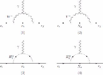

Figure 1.  Feynman diagrams at the one-loop order for $e_i \rightarrow e_j \gamma$ decays in the unitary gauge.

With ordinary charged leptons, $m_{e_i}\gg m_{e_j}, i > j$ leads to $\left| {\cal{D}}_{(ji)R}\right| \gg \left| {\cal{D}}_{(ji)L}\right|$; therefore, we usually ignore ${\cal{D}}_{(ji)L}$ in Eq. (19) when examining ${\rm{Br}}(e_i\rightarrow e_j\gamma)$. The notations corresponding to the contributions to $e_i\rightarrow e_j\gamma$ decays are

The third contributor (${\rm{Br}}^{\nu W}$) consists of only the same particles as those that appear in the SM. We investigate the contributions of these components to ${\rm{Br}}^{\rm Total}(e_i\rightarrow e_j\gamma)$ in the numerical calculation.

For convenience, when investigating the LFVHDs of the SM-like Higgs boson $h^0_1\rightarrow e_i^{\pm}e_j^{\mp}$, we use the scalar factors ${\rm{C}}_{(ij)L}$ and ${\rm{C}}_{(ij)R}$. Therefore, the effective Lagrangian of these decays is

Based on the couplings listed in Table 3, the one-loop Feynman diagrams contributing to these LFVHD amplitudes in the unitary gauge are shown in Fig. 2. Inevitably, the scalar factors ${\rm{C}}_{(ij)L,R}$ arise from the loop contributions, and we only consider all corrections at the one-loop order.

Figure 2.  Feynman diagrams at the one-loop order of $h_1^0 \rightarrow \mu \tau$ decays in the unitary gauge.

The partial width of $h^0_1\rightarrow e_i^{\pm}e_j^{\mp}$ is

We use the following conditions for external momentum: $p^2_{i,j}=m^2_{i,j}$, $(p_i+p_j)^2=m^2_{h^0_1}$, and $m^2_{h^0_1}\gg m^2_{i,j}$, which leads to the branching ratio of $h^0_1\rightarrow e_i^{\pm}e_j^{\mp}$ decays being given as

where $\Gamma^{\rm{total}}_{h^0_1}\simeq 4.1\times 10^{-3}\; {\rm{GeV}}$, as shown in Refs. [2, 58].

The factors corresponding to the diagrams of Fig. 2 are given in Appendix D. To calculate the total amplitude for the LFVHDs in this model, we separate them into two parts: ${\rm{C}}_{(ij)L,R}^\nu$ for the contributions of active neutrinos, and ${\rm{C}}_{(ij)L,R}^{N}$ for the contributions of exotic leptons. They are

and

The total factor for the LFVHD process is

In ${\rm{C}} _ {(ij) L, R}$, there are divergence terms, which are implicit in Passarino-Veltman (PV) functions ($B_0^{(n)},\,B_1^{(n)}, n=1,2$), as shown in Appendix D. However, we can use the techniques mentioned in Refs. [40, 57] to separate the divergences and finite parts in each factor. It is clear that the divergence parts are eliminated because their sum is zero, and the contributions of the remaining finite part are shown in the following numerical investigation.

We use the following well-known experimental parameters [1, 2]: the charged lepton masses $m_e=5\times 10^{-4} {\rm{GeV}}$, $m_\mu=$ 0.105 GeV, and $m_\tau=$ 1.776 GeV, the SM-like Higgs mass $m_{h^0_1}=$ 125.1 MeV, the mass of the W boson $m_W=$ 80.385 GeV, and the gauge coupling of $S U(2)_L$ symmetry $g \simeq 0.651$.

In this model, we can give the relationship of the neutral gauge boson outside the SM as $m_Z'^2= \dfrac{g^2v_3^2c_W^2}{3-4s_W^2}$. However, $m_Z'\geq 4.0\,{\rm{TeV}}$ is the limit given by Refs. [8, 9], resulting in $v_3\geq 10.1\, {\rm{TeV}}$. At the LHC$@13{\rm{TeV}}$, we can choose $m_V=4.5[{\rm{TeV}}]$ to satisfy the above conditions. This value of $m_V$ is suitable and shown in the numerical investigation below. The mixing angle between light VEVs is chosen as $\dfrac{1}{60}\leq t_{12}\leq 3.5$, in accordance with Refs. [43, 59]. However, the LFVHDs in this model depend very little on the change in $t_{12}$; hence, we choose $t_{12}=0.5$ for the following investigations. Furthermore, the $s_\delta$ parameter is an important parameter of the THDM. In section III, we show that the couplings of $h^0_1$ are similar to those in the SM when $s_\delta \rightarrow 0$, and combined with the condition used to satisfy all THDMs, $c_\delta > 0.99$, according to the results shown in Ref. [60], we choose $\left| s_\delta\right| < 0.14$. With the arange of $\left| s_\delta\right|$, the model under consideration also predicts the existence of a large signal of $h_1^0 \rightarrow Z \gamma$. This has been detailed in a recent study [43].

The absolute values of all Yukawa and Higgs self couplings should be less than $\sqrt{4\pi}$ and $4\pi$, respectively. In addition to the parameters that can impose conditions on determining value domains, we choose the set of free parameters for this model as $\lambda_1,\,\tilde{\lambda}_{12},\, s_\delta, \,m_{h_2^0},\,m_{N_1},\,m_{N_2}$, and $m_{H^\pm_2}$.

Therefore, the dependent parameters are given below.

and $\lambda_{13}$ is given using the invariance trace of the squared mass matrices in Eq. (A9) in Appendix A,

Regarding the parameters of active neutrinos, we use the recent results of experiments shown in Refs. [1, 2, 56]. $\Delta m_{21}^2=7.55 \times 10^{-5} {\rm{eV}}^2$, $\Delta m_{31}^2=2.424 \times 10^{-3} {\rm{eV}}^2$, $\sin^2 \theta^\nu_{12}=0.32$, $\sin^2 \theta^\nu_{23}=0.547$, and $\sin^2 \theta^\nu_{13}=0.0216$.

The mixing matrix of active neutrinos is derived from $U^{\rm MNPS}$ when we ignore a very small deviation [61]. That way, $U \equiv U^L=U (\theta_{12}^\nu,\theta_{13}^\nu,\theta_{23}^\nu)$, and $U^\dagger=U^\dagger (\theta_{12}^\nu,\theta_{13}^\nu,\theta_{23}^\nu)$, where $\theta_{ij}^\nu$ are the mixing angles of active neutrinos. The parameterized form of the U matrix is

Exotic leptons are also mixed in a common way based on Eq. (30) by choosing $V^L \equiv U^L(\theta_{12}^N,\theta_{13}^N,\theta_{23}^N)$, where $\theta_{ij}^N$ are the mixing angles of exotic leptons. The parameterization of $V^L$ is chosen so that LFV decays can be obtained with large signals. According to that criterion, we can provide cases corresponding to the large mixing angle of exotic leptons, for example, $V^L \equiv U^L\left(\dfrac{\pi}{4},\dfrac{\pi}{4},\dfrac{\pi}{4}\right)$, $V^L \equiv U^L\left(\dfrac{\pi}{4},\dfrac{\pi}{4},-\dfrac{\pi}{4}\right)$, and $V^L \equiv U^L\left(\dfrac{\pi}{4},0,0\right)$. The other cases only change minus signs in thetotal amplitudes without changing the final result of the branching ratios of the LFVHD process.

The analytical results for the components of $e_i \rightarrow e_j \gamma$ are given with Eq. (21). Using these, we give the parameter space domains of this model satisfying the experimental limits of $e_i \rightarrow e_j \gamma$ decays.

Among the cLFV, $\mu \rightarrow e \gamma$ has the strictest experimental limit; therefore, in the regions of parameter space where $\mu \rightarrow e \gamma$ satisfies the experimental limits, the $\tau \rightarrow e \gamma$ and $\tau \rightarrow \mu \gamma$ decays also satisfy them. This result has also been shown in similar studies mentioned in Refs. [19, 57]. To avoid unnecessary investigations, we only introduce parameter regions satisfying the experimental conditions of $\mu \rightarrow e \gamma$ in different mixing cases of exotic leptons. These domains are ensured to match for the remaining two cLFV.

Without loss of generality, we can investigate the $V^L_{ab} = U^L_{ab}(\pi/4,\pi/4,\pi/4)$ case. Then, the components of the $\mu \rightarrow e\gamma$ decay are given, as shown in Fig. 3.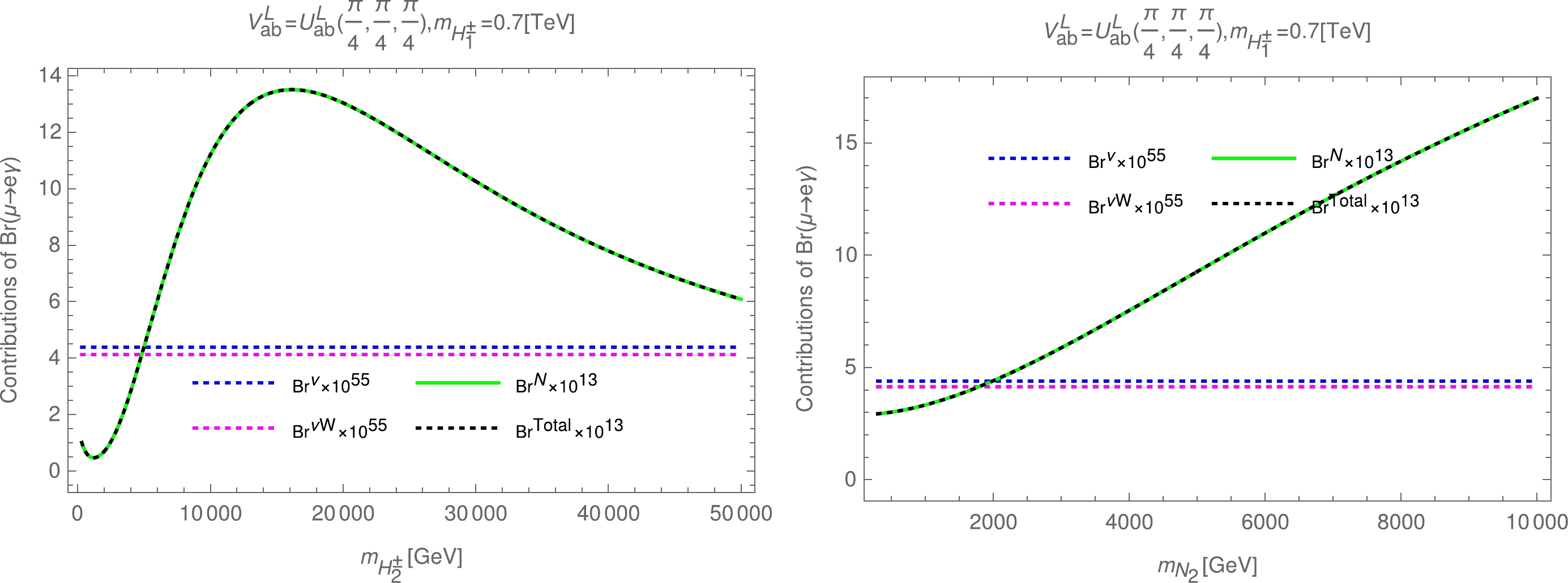

Figure 3.  (color online) Contributions to the $\mu \rightarrow e\gamma$ decay in the case of $V^L_{ab} = U^L_{ab}(\pi/4,\pi/4,\pi/4)$ with respect to $m_{H^\pm_2}$ (left panel) and $m_{N_2}$ (right panel).

As a result, ${\rm{Br}}^\nu$ and ${\rm{Br}}^{\nu W}$ give a very small contribution compared with ${\rm{Br}}^{\rm Total}$, whereas ${\rm{Br}}^N$ of the exotic leptons is close to the main contribution. Therefore, we can ignore small contributions in later calculations. In particular, with the choice of the largest mixing parameters of the exotic leptons, significant signals for the $\mu \rightarrow e\gamma$ decay are at approximately $m_{H^\pm_2}<8.0\; {\rm{TeV}}$ (left panel) and $m_{N_2}<2.0\; {\rm{TeV}}$ (right panel).

The anomalous magnetic moments of electrons and muons $a_{e,\mu}=(g_{e,\mu}-2)/2$ mentioned earlier are of interest now. However, they are closely related to the decays of charged leptons. From Eqs. (19) and (20), we can write

where ${\cal{D}}^\nu_{(ij)R} ={\cal{D}}^{\nu_a WW}_{(ij)R}+{\cal{D}}^{\nu_a H_1H_1}_{(ij)R},\; {\cal{D}}^{N}_{(ij)R}={\cal{D}}^{N_a VV}_{(ij)R}+{\cal{D}}^{N_a H_2H_2}_{(ij)R}$, and using the results in Appendix C, we have

According to the results shown in Fig. 3, the contribution of active neutrinos is very small compared with that of neutral leptons. Therefore, the contributions to the anomalous magnetic moments of muons and the cLFV are

With the form of the matrix $V^L_{ab}$ chosen as Eq. (30), ${\cal{D}}_{(21)R}$ and ${\cal{D}}_{(22)R}$ are always of the same order. Furthermore, in the limit ${\rm{Br}}(\mu \rightarrow e\gamma)\leq 4.2 \times 10^{-13}$, the condition $|{\cal{D}}_{(21)R}|\leq {\cal{O}}(10^{-13})$ is required. Hence, $|{\cal{D}}_{(22)R}|\leq {\cal{O}}(10^{-13})$ [48], resulting in $|\Delta a_\mu|\leq {\cal{O}}(10^{-13})$. This is a very small signal compared with the current experimental limit (${\cal{O}}(10^{-9})$); therefore, the signal of $|\Delta a_\mu|$ is negligible in the parameter space regions in which we investigate the cLFV.

Based on Refs. [8, 9], in this model ($\beta =- {1}/{\sqrt{3}}$), we have the limit on the heavy VEV of $v_3 \geq 10.1 \; {\rm{TeV}}$, resulting in $m_V\geq 3.8 \; {\rm{TeV}}$. Correspondingly, at the expected energy scale of the LHC, $v_3 \sim 13 \; {\rm{TeV}}$, and hence $m_V\sim 4.5 \; {\rm{TeV}}$. To select the appropriate region of $m_V$, we fix $m_{N_1}=13\; {\rm{TeV}}$. Then, the dependence of ${\rm{Br}}(\mu \rightarrow e\gamma)$ on $m_V$ and $m_{H^\pm_2}$ or $m_{N_2}$ is given as shown in Fig. 4.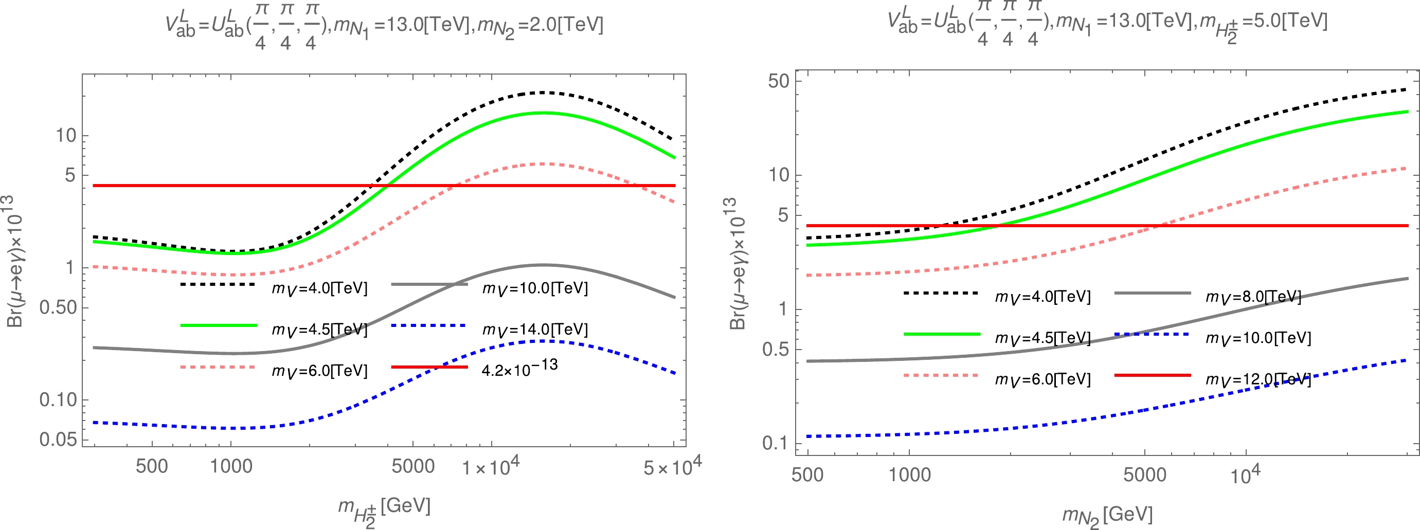

Figure 4.  (color online) Dependence of ${\rm{Br}}(\mu \rightarrow e\gamma)$ on $m_{V}$ and $m_{H^\pm_2}$ (left) or $m_{N_2}$ (right) in the case of $V^L_{ab} = U^L_{ab}(\pi/4,\pi/4,\pi/4)$.

As indicated by the result in Fig. 4, the larger the value of $m_V$, the better the experimental limits on ${\rm{Br}}(\mu \rightarrow e\gamma)$ are satisfied. However, a small value of ${\rm{Br}}(\mu \rightarrow e\gamma)$ may be considered undesirable because this makes it difficult to detect experimentally. We find the best fit when choosing $m_V=4.5\; {\rm{TeV}}$ to perform the numerical investigation of lepton-flavor-violating decays.

The results of the numerical survey show that ${\rm{Br}}(\mu \rightarrow e\gamma)$ depends very little on the change in $t_{12}$. Therefore, to ensure the limit $\dfrac{1}{60}\leq t_{12}\leq 3.5$, we always choose the fixed value $t_{12}=0.5$. Combined with the fixed selection of $m_V=4.5\; {\rm{TeV}}$, the dependence of ${\rm{Br}}(\mu \rightarrow e\gamma)$ on $m_{H^\pm_2}$ and the masses of exotic leptons is given in Fig. 5.

Figure 5.  (color online) Dependence of ${\rm{Br}}(\mu \rightarrow e\gamma)$ on $m_{H^\pm_2}$ (first row) and contour plots of ${\rm{Br}}(\mu \rightarrow e\gamma)$ (second row) as functions of $m_{H^\pm_2}$ and $m_{N_1}$ (left panel) or $m_{H^\pm_2}$ and $m_{N_2}$ (right panel) in the case of $V^L_{ab} = U^L_{ab}(\pi/4,\pi/4,\pi/4)$.

In Fig. 5, we consider the dependence of ${\rm{Br}}(\mu \rightarrow e\gamma)$ on $m_{H^\pm_2}$ and $m_{N_1}$ or $m_{N_2}$. In the first row, we show the parameter space region of ${\rm{Br}}(\mu \rightarrow e\gamma)< 4.2\times 10^{-13}$ in the domain $1.0 \; {\rm{TeV}} \leq m_{H^\pm_2}\leq 7.0\; {\rm{TeV}}$ with two cases: i) $m_{N_1}=2.0\; {\rm{TeV}}$, and $m_{N_2}$ is approximately $13.0 \; {\rm{TeV}}$ (left), and ii) $m_{N_2}=2.0\; {\rm{TeV}}$ and $m_{N_1}$ is approximately $13.0 \; {\rm{TeV}}$ (right). In each of these parameter regions, the value curves of ${\rm{Br}}(\mu \rightarrow e\gamma)$ decrease as $m_{N_1}$ increases (left) or increase as $m_{N_2}$ increases (right). Therefore, the contributions of $m_{N_1}$ and $m_{N_2}$ to ${\rm{Br}}(\mu \rightarrow e\gamma)$ in this case can presented in short form as follows: $m_{N_2}$ has an increasing effect, whereas $m_{N_1}$ has a decreasing effect. This property is also true for the other two decays, $\tau \rightarrow e\gamma$ and $\tau \rightarrow \mu\gamma$. The combination of these properties leads to the existence of regions of parameter space that satisfy the experimental limits of $e_i \rightarrow e_j\gamma$ decays when one exotic lepton has a mass of approximately $2.0 \; {\rm{TeV}}$ and another is approximately $13.0 \; {\rm{TeV}}$. These significant space regions are shown to correspond to the colorless part shown in the second row of Fig. 5.

In the same manner, we can obtain the results of the remaining typical cases of exotic lepton mixing, as shown in Fig. 6.

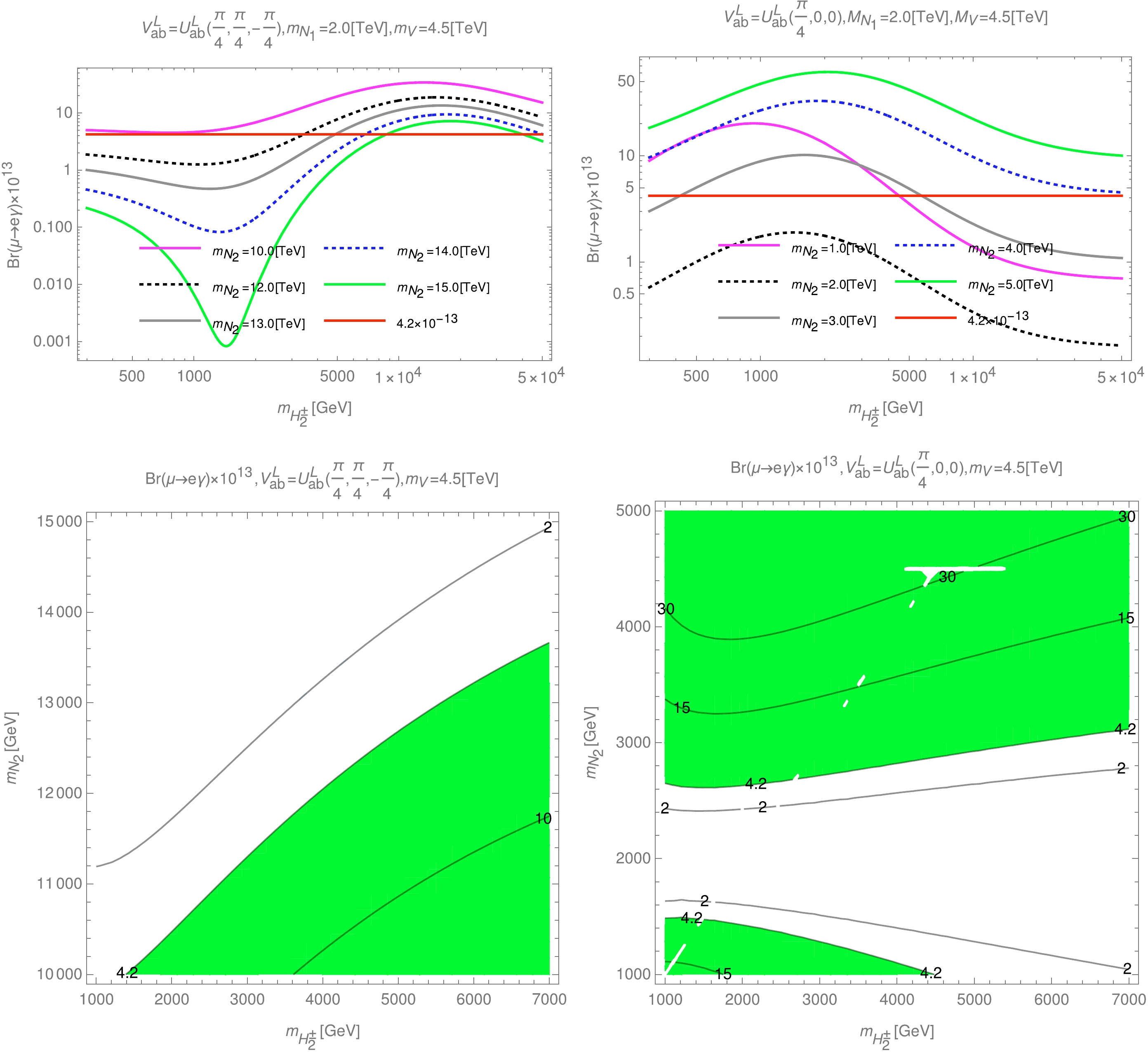
Figure 6.  (color online) Dependence of ${\rm{Br}}(\mu \rightarrow e\gamma)$ on $m_{H^\pm_2}$ (first row) and contour plots of ${\rm{Br}}(\mu \rightarrow e\gamma)$ as functions of $m_{H^\pm_2}$ and $m_{N_2}$ (second row) in the case of $V^L_{ab} = U^L_{ab}(\pi/4,\pi/4,-\pi/4)$ (left panel) or in the case of $V^L_{ab} = U^L_{ab}(\pi/4,0,0)$ (right panel).

In both the $V^L_{ab} = U^L_{ab}(\pi/4,\pi/4,-\pi/4)$ and $V^L_{ab} = U^L_{ab}(\pi/ 4,0,0)$ cases, we choose $m_{N_1}=2.0 \; {\rm{TeV}}$. The allowed domains of the $e_i \rightarrow e_j\gamma$ decays are shown in the second row of Fig. 6. We find that the $V^L_{ab} = U^L_{ab}(\pi/4,\pi/4,-\pi/4)$ and $V^L_{ab} = U^L_{ab}(\pi/4,\pi/4,\pi/4)$ cases give nearly the same results when the role of $m_{N_1}$ and $m_{N_2}$ are swapped (see the left panels in the second row of Fig. 5 and Fig. 6). This is also a typical feature of this model; therefore, the numerical investigation below is mainly performed according to the dependence on $m_{H^\pm_2}$ and $m_{N_2}$.

The three LFVHDs have an experimental upper limit as given in Eq. (2). We can investigate these decays in regions of the parameter space that satisfy $e_i \rightarrow e_j\gamma$ decays. From Eq. (27) and Appendix D, we realize that $C_{(ij)L}\sim m_j,\,C_{(ij)R}\sim m_i$ combined with $m_\tau \gg m_\mu \gg m_e$; hence, ${\rm{Br}}(h^0_1 \rightarrow \mu\tau)$ can receive the largest signal among the LFVHDs in this model. Therefore, we focus on finding the large signal of the $h^0_1 \rightarrow \mu\tau$ decay in the following surveys.

We use Eq. (24) to investigate the dependence of ${\rm{Br}}(h^0_1 \rightarrow \mu\tau)$ on $s_\delta$ in the case of $V^L_{ab} = U^L_{ab}(\pi/4,\pi/4,\pi/4)$, ($s_\delta$-specific parameter for the THDM), and the results are given as shown in Fig. 7. Clearly, ${\rm{Br}}(h^0_1 \rightarrow \mu\tau)$ increases proportionally to the absolute value of $s_\delta$. Therefore, in the limited range $0<\left| s_\delta \right| <0.14$, ${\rm{Br}}(h^0_1 \rightarrow \mu\tau)$ can give the largest signal when $\left| s_\delta \right| \rightarrow 0.14$.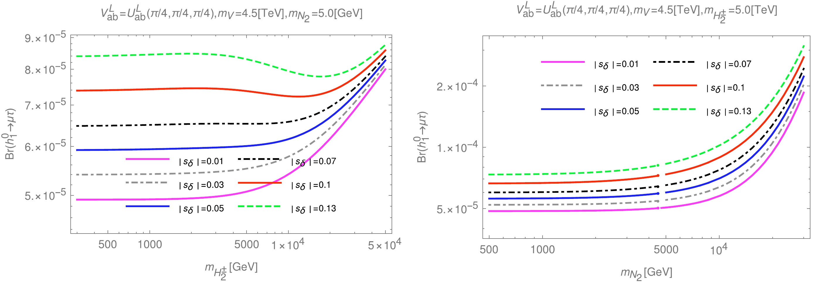

Figure 7.  (color online) Dependence of ${\rm{Br}}(h^0_1 \rightarrow \mu\tau)$ on $m_{H^\pm_2}$ (left) or $m_{N_2}$ (right) in the case of $V^L_{ab} = U^L_{ab}(\pi/4,\pi/4,\pi/4)$.

In the case of $V^L_{ab} = U^L_{ab}(\pi/4,\pi/4,\pi/4)$, to find the possible parameter space for the large signal of ${\rm{Br}}(h^0_1 \rightarrow \mu\tau)$, we choose the fixed value $\left| s_\delta \right| = 0.13$. Then, the change in ${\rm{Br}}(h^0_1 \rightarrow \mu\tau)$ according to $m_{H^\pm_2}$ and $m_{N_2}$ is shown in Fig. 8.

Figure 8.  (color online) ${\rm{Br}}(h^0_1 \rightarrow \mu\tau)$ as a function of $m_{H^\pm_2}$ in the case of $V^L_{ab} = U^L_{ab}(\pi/4,\pi/4,\pi/4)$ (left) and density plots of ${\rm{Br}}(h^0_1 \rightarrow \mu\tau)$ as a function of $m_{H^\pm_2}$ and $m_{N_2}$ (right). The black curves in the right panel show the constant values of ${\rm{Br}}(\mu \rightarrow e\gamma)\times 10^{13}$.

As a result, ${\rm{Br}}(h^0_1 \rightarrow \mu\tau)$ increases with $m_{N_2}$, as shown in the left part of Fig. 8. However, the part of the parameter space is significant; the part in which the experimental limits of ${\rm{Br}}(\mu \rightarrow e\gamma)$ are satisfied is shown in the interval between the $4.2$ curves in the right part of Fig. 8. We show that the largest value ${\rm{Br}}(h^0_1 \rightarrow \mu\tau)$ can achieve in this case is approximately ${\cal{O}}(10^{-5})$.

In a similar manner, we investigate ${\rm{Br}}(h^0_1 \rightarrow e\mu)$ and ${\rm{Br}}(h^0_1 \rightarrow e\tau)$ in the region of parameter space given in Fig. 8. The results are shown in Fig. 9.

Figure 9.  (color online) Density plots of ${\rm{Br}}(h^0_1 \rightarrow e\mu)$ (left) and ${\rm{Br}}(h^0_1 \rightarrow e\tau)$ (right) as a function of $m_{H^\pm_2}$ and $m_{N_2}$ in the case of $V^L_{ab} = U^L_{ab}(\pi/4,\pi/4,\pi/4)$. The black curves show the constant values of ${\rm{Br}}(\mu \rightarrow e\gamma)\times 10^{13}$.

The results obtained for ${\rm{Br}}(h^0_1 \rightarrow e\mu)$ and ${\rm{Br}}(h^0_1 \rightarrow e\tau)$ are below the upper bound of the experimental limits mentioned in Eq. (2). In addition, these values are smaller than the corresponding values of ${\rm{Br}}(h^0_1 \rightarrow \mu \tau)$. Therefore, we are only interested in the large signal that ${\rm{Br}}(h^0_1 \rightarrow \mu \tau)$ can achieve in the other investigated cases.

For the other cases of mixed matrix exotic leptons, $V^L_{ab} = U^L_{ab}(\pi/4,\pi/4,-\pi/4)$ and $V^L_{ab} = U^L_{ab}(\pi/4,0,0)$, we also show parameter space domains that can give large signals of ${\rm{Br}}(h^0_1 \rightarrow \mu\tau)$ and satisfy the experimental conditions of $(e_i \rightarrow e_j\gamma)$ decays, as shown in Fig. 10.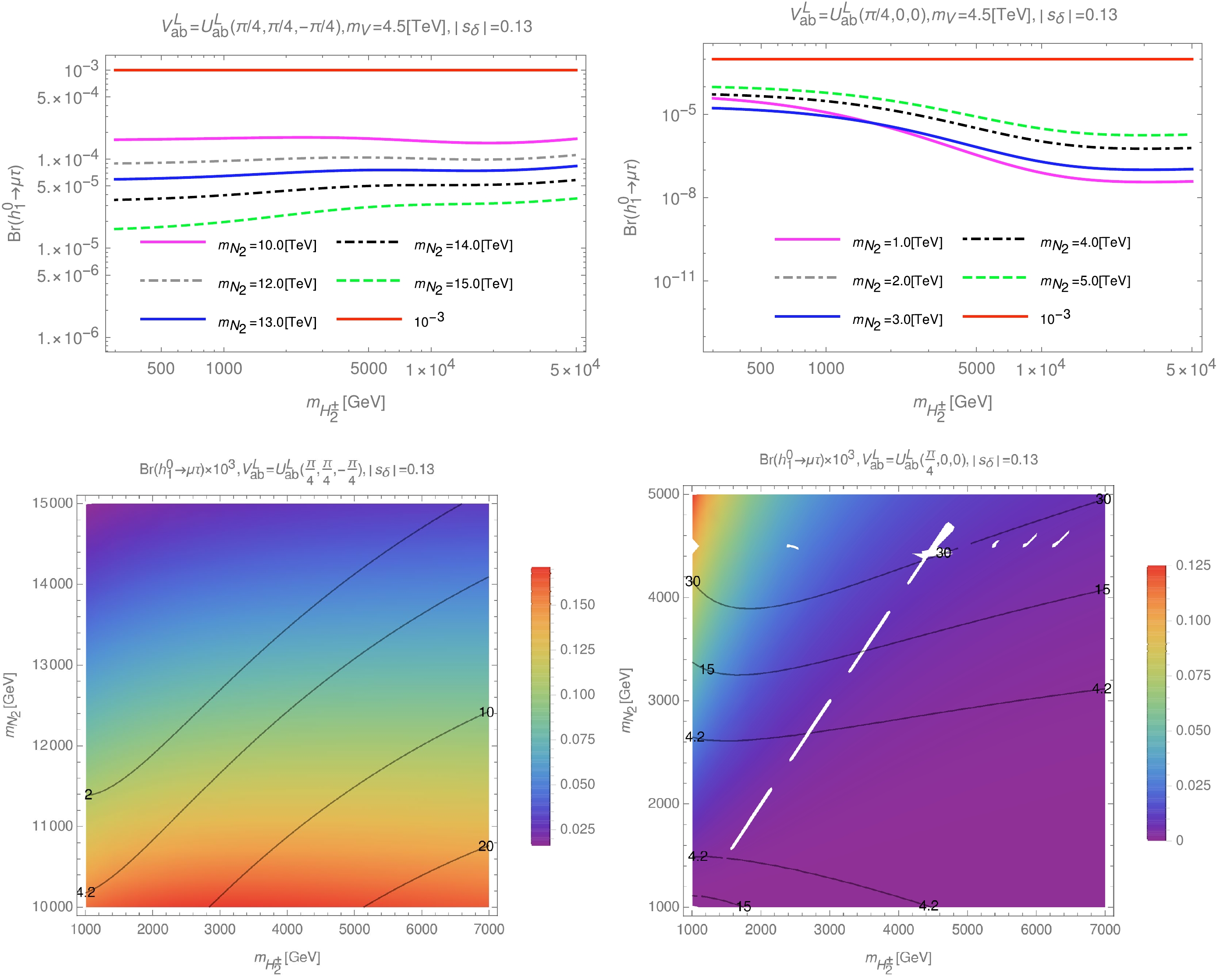

Figure 10.  (color online) Dependence of ${\rm{Br}}(h^0_1 \rightarrow \mu\tau)$ on $m_{H^\pm_2}$ (first row), and density plots of ${\rm{Br}}(h^0_1 \rightarrow \mu\tau)$ as a function of $m_{H^\pm_2}$ and $m_{N_2}$ (second row) in the case of $V^L_{ab} = U^L_{ab}(\pi/4,\pi/4,-\pi/4)$ (left panel) or in the case of $V^L_{ab} = U^L_{ab}(\pi/4,0,0)$ (right panel). The black curves in the second row show the constant values of ${\rm{Br}}(\mu \rightarrow e\gamma)\times 10^{13}$.

With $V^L_{ab} = U^L_{ab}(\pi/4,0,0)$, ${\rm{Br}}(h^0_1 \rightarrow \mu\tau)$ can reach approximately $10^{-4}$; however, in space domains satisfying the experimental limits of the $(\mu \rightarrow e\gamma)$ decay, ${\rm{Br}}(h^0_1 \rightarrow \mu\tau)$ can only reach a value of less than $10^{-5}$. This result is entirely consistent with the corresponding object, which was previously published in Ref. [40]. When the mixing matrix of exotic leptons has the form $V^L_{ab} = U^L_{ab}(\pi/4,\pi/4,-\pi/4)$, we can obtain allowed parameter space domains that can give signals of ${\rm{Br}}(h^0_1 \rightarrow \mu\tau)$ of up to $10^{-4}$. This is the largest signal of ${\rm{Br}}(h^0_1 \rightarrow \mu\tau)$ that we can predict in this model and is also close to the upper limit of this decay ($10^{-3}$), as shown in Refs. [1, 2, 56]. It should be recalled that we previously showed the existence the large signal of ${\rm{Br}}(h^0_1 \rightarrow Z\gamma)$ ($1.0\leq {\rm{R}}_{Z\gamma/\gamma \gamma}\leq 2.0$) in Ref. [43]. Although, the two decays $h^0_1 \rightarrow \mu\tau$ and $h^0_1 \rightarrow Z\gamma$ have different private parts, the common parts are given in the same corresponding form. For example, the common couplings $hV^-V^+ (V^+\equiv W^+,V^+),\, hf\overline{f} (f\equiv e_a),\,$$hV^-S^+ (S^+\equiv H_{1,2}^+),\, hS^-S^+ (S^+\equiv H_{1,2}^+)$ are given the same form for each decay, the dependent parameters $\lambda_2, \lambda_{12}, \lambda_{13}, \lambda_{23}$ are given in the same corresponding form, and free parameters, such as $\lambda_1, s_\delta, t_{12}, M_V, ...$, are selected corresponding to the same value domains when examining the two decays $h \rightarrow e_ie_j$ and $h \rightarrow Z\gamma$... All common value domains are chosen to be the same. Therefore, we believe that there are parameter space domains of this model in which both the $h \rightarrow e_ie_j$ and $h \rightarrow Z\gamma$ decays achieve large signals. These are the decays of interest of the SM-like Higgs boson, and their signals are expected to be detectable from large accelerators to confirm the influence of this model.

The 3-3-1 model with neutral leptons gives a diverse Higgs mass spectrum when using the Higgs potential in a general form (Eq. (7)). Applying the same technique as Refs. [32, 43], we can identify two neutral Higgs corresponding to those of the THDM. This causes the 331NL model to inherit several features of the THDM, as mentioned in Refs. [32, 62].

We find the contribution of exotic leptons to be the main components of $(e_i \rightarrow e_j\gamma)$ decays at the $13 \; {\rm{TeV}}$ scale of the LHC, leading to constraints on the masses of some particles, such as $m_V \sim$ 4.5 TeV, $m_{H_1^\pm} \sim$ 0.7 TeV, and $m_{h_2^0} \sim$ 1.5 TeV. Via numerical investigation, we show that the parameter space regions satisfying the experimental limits of $(e_i \rightarrow e_j\gamma)$ are highly dependent on the mixing of exotic leptons. However, two cases, $V^L_{ab} = U^L_{ab}(\pi/4,\pi/4, \pi/4)$ and $V^L_{ab} = U^L_{ab}(\pi/4,\pi/4,-\pi/4)$, can give roughly the same result when the roles of $m_{N_1}$ and $m_{N_2}$ are swapped. The allowed space regions in this part are all given when fixed at $m_V=4.5 \; {\rm{TeV}}$, exotic leptons have masses of approximately $2.0 \; {\rm{TeV}}$, or another exotic lepton is at $13.0 \; {\rm{TeV}}$.

Although, the forms of the mixing matrix of exotic leptons do not affect the absolute value of the total amplitude of the $h^0_1 \rightarrow \mu\tau$ decay, they affect the regions of parameter space where ${\rm{Br}}(e_i \rightarrow e_j\gamma)$ are satisfied. This motivates us to find the large signal of ${\rm{Br}}(h^0_1 \rightarrow \mu\tau)$ in the allowed space of $e_i \rightarrow e_j\gamma$ decays.

Performing a numerical investigation, we show that ${\rm{Br}}(h^0_1 \rightarrow \mu\tau)$ is always less than $10^{-5}$ in the case of $V^L_{ab} = U^L_{ab}(\pi/4,0,0)$, which is in full agreement with the previously published results in Ref. [40]. We also show that ${\rm{Br}}(h^0_1 \rightarrow \mu\tau)$ always increases proportionally to $\left| s_\delta \right|$ in all cases of $V^L_{ab}$. Therefore, in the range of values $0<\left| s_\delta \right|<0.14$, ${\rm{Br}}(h^0_1 \rightarrow \mu\tau)$ can be obtain large values when $\left| s_\delta \right| \rightarrow 0.14$. Combined with the results shown in Ref. [43], ${\rm{Br}}(h^0_1 \rightarrow Z\gamma)$ can also give large signals in this range of values. Hence, we can expect to obtain regions of parameter space for the existence of large signals from both ${\rm{Br}}(h^0_1 \rightarrow \mu\tau)$ and ${\rm{Br}}(h^0_1 \rightarrow Z\gamma)$ in this model. Furthermore, we also predict that the large signal of ${\rm{Br}}(h^0_1 \rightarrow \mu\tau)$ can reach $10^{-4}$ in the case of $V^L_{ab} = U^L_{ab}(\pi/4,\pi/4,-\pi/4)$. This signal is close to the upper limit of this channel and is expected to be detectable using large accelerators.

Higgs bosons

From Eq. (7), the minimum conditions of the Higgs potential are

There are two Goldstone bosons, $G^{\pm}_W$ and $G^{\pm}_V$, of the respective singly charged gauge bosons $W^{\pm}$ and $V^{\pm}$. Two other massive singly charged Higgs have the masses

The relationship between the two flavor and mass bases of the singly charged Higgs is

where $s_{ij}\equiv\sin\beta_{ij}$, $c_{ij}\equiv\cos\beta_{ij}$, $t_{12}\equiv\tan\beta_{12}= \dfrac{v_2}{v_1}, ~~ t_{13}\equiv \tan\beta_{13}= \dfrac{v_1}{v_3},\; t_{23}\equiv\tan\beta_{23}=\dfrac{v_2}{v_3}$,

With the components of the selected scalar fields (Eq. (6)), we initially obtain $5$ real scalars, namely, $S_1, S_2, S_3, S_2'. S_3'$. In the final state, similar to Refs. [40, 63], we obtain four massive Higgs and a Goldstone boson ($G_{U}$) corresponding to the gauge boson U. A heavy neutral Higgs mixed with $G_{U}$ on the original basis ($S'_2, S'_3$) is

and the mass of $h^0_4$ is given as

The remainders are three neutral Higgs whose mass mixing matrix on the flavor basis ($S_1,S_2,S_3$) is

Among the three neutral Higgs mentioned in Eq. (A6), the lightest, $h^0_1$, is identified with the Higgs boson in the SM (known as the SM-like Higgs boson). To avoid the tree level contributions of the SM-like Higgs boson to the flavor changing neutral currents in the quark sector, we used the aligned limit introduced in Refs. [32, 43], namely

For simplicity, we choose f and $\lambda_{23}$ as functions of the remainder. Thus, the mass matrix of the Higgs in Eq. (A6) becomes

As a result, $S_3\equiv h^0_3$ is a physical CP-even neutral Higgs boson with mass $m^2_{h^0_3}= \lambda_{13}v_2^2 +2\lambda_3 v_3^2$. The sub-matrix $2\times 2$ in Eq. (A8) is denoted as $M'^2_h$, which is diagonalized as follows:

where

Using the techniques described in Refs. [32, 43], we find that the masses of neutral Higgs depend on the mixing angle δ, which is a characteristic parameter of the THDM. As mentioned in Ref. [60], this parameter constrains $c_\delta >0.99$ for all THDMs, resulting in $\left| s_\delta \right| <0.14$.

The components $M_{{\rm{ij}}}$ of a $2\times 2$ matrix are formed from the sub-matrix of ${\cal{M}}^2_h$ after rotating the angle $\beta_{12}$.

We also have

The lightest $h^0_1$ is the SM-like Higgs boson found at the LHC. From Eqs. (44) and (45), we can see that $\tan2\delta= \dfrac{2M^2_{12}}{M^2_{22} -M^2_{11}}= {\cal{O}}\left(\dfrac{v^2}{v_3^2}\right) \simeq0$ when $v^2\ll v_3^2$. In this limit, $m^2_{h}= M^2_{22} + v^2\times$ ${\cal{O}}\left(\dfrac{v^2}{v_3^2}\right)\sim M^2_{22}$, while $m^2_{h^0_2}= M^2_{11} + v^2 \times {\cal{O}}\left(\dfrac{v^2}{v_3^2}\right) \simeq M^2_{11}$. In the next section, we see more explicitly that the couplings of $h_1^0$ are the same as those given in the SM in the limit $\delta\rightarrow 0$.

Using the invariance trace of the squared mass matrices in Eq. (A9), we have

where $\lambda_{13}$ can be written as

The other Higgs self couplings are given in Table 3. They should satisfy all constraints discussed in literature to guarantee the pertubative limits, the vacuum stability of the Higgs potential [64], and the positive squared masses of all Higgs bosons.

Gauge bosons

$S U(3)_L\otimes U(1)_X$ includes eight generators, $T^a$ (a=1,8), of $S U(3)_L$ and a generator $T^9$ of $U(1)_X$, corresponding to eight gauge bosons, $W^a_{\mu}$, and $X_{\mu}$ of $U(1)_X$. The respective covariant derivative is

The Gell-Mann matrices are denoted as $\lambda_a$, and we have $T^a=\dfrac{1}{2}\lambda_a,-\dfrac{1}{2}\lambda_a^T$, or $0$ depending on the triplet, antitriplet, or singlet representation of the $S U(3)_L$ that $T^a$ acts on. $T^9$ is defined as $T^9=\dfrac{1}{\sqrt{6}}$, and X is the $U(1)_X$ charge of the field it acts on. We also define $W_\mu^+ = \dfrac{1}{\sqrt{2}}(W_\mu^1- {\rm i} W_\mu^2)$, $V_\mu^-=\dfrac{1}{\sqrt{2}}(W_\mu^6-{\rm i} W_\mu^7)$, and $U_\mu^0=\dfrac{1}{\sqrt{2}}(W_\mu^4- {\rm i} W_\mu^5)$:

The masses of these gauge bosons are

where we use the relation $v_1^2+v_2^2=v^2\equiv 246^2 {\rm{GeV^2}}$ so that the mass of the W-boson in the 331NL model matches the corresponding value in the SM.

The three remaining neutral gauge bosons, $A_\mu$, $Z_\mu$, and $Z^\prime_\mu$, couple to the fermions in a diagonal basis, as shown in Ref. [43]. These couplings do not correlate with LFV decays; hence, we do not mention them in this paper.

To calculate the contributions at the one-loop order of the Feynman diagrams in Figs. 1 and 2, we use the PV functions mentioned in Ref. [65]. By introducing the notations $D_0=k^2-M_0^2+{\rm i}\delta$, $D_1=(k-p_1)^2- M_{1}^2+ {\rm i}\delta$, and $D_2=(k+p_2)^2-M_2^2+{\rm i}\delta$, where δ is infinitesimally a positive real quantity, we have

where $n=1,2$, $D=4-2\epsilon \leq 4$ is the dimension of the integral, while $\; M_0,\; M_1,\; M_2$ stand for the masses of virtual particles in the loops. We also assume $p^2_1=m^2_{1},\; p^2_2=m^2_{2}$ for external fermions. The tensor integrals are

where $A_0$, $B^{(n)}_{0,1}$, $B^{(12)}_{n}$, and $C_{0,n}, C_{mn}$ are PV functions. It is well-known that $C_{0,n}, C_{mn}$ are finite while the remains are divergent. We denote

where $\gamma_{\rm E}$ is the Euler constant.

Using the technique mentioned in Ref. [19], we can show the divergent parts of the above PV functions as

Apart from the divergent parts, the rest of these functions are finite.

Thus, the above PV functions can be written in form

where $a_0(M), \,\,b^{(n)}_{0,1}, \,\, b^{(12)}_{0,1,2}$ are finite parts and have a specific form defined in Ref. [19] for $e_i \rightarrow e_j \gamma$ decays and Ref. [20] for the $h^0_1 \rightarrow \mu \tau$ decay.

We use the techniques shown in [19, 57] to give the factors at the one-loop order of $e_i \rightarrow e_j\gamma$ decays. The PV functions obey the rules shown in [65] and have a common set of variables ($p_k^2,m_1^2,m_2^2,m_3^2$), with $p_k^2=m_{e_i}^2,0,m_{e_j}^2$ related to external momenta, and $m_1^2,m_2^2,m_3^2$ related to masses in the loop of Fig. 1. For brevity, we use the notations $C_{0,n} \equiv C_{0,n}(p_k^2,m_1^2,m_2^2,m_3^2)$ and $C_{mn} \equiv C_{mn}(p_k^2, m_1^2, m_2^2,m_3^2); m,n=1,2$ in the analytic formulas below.

The factors of diagram (1) in Fig. 1.

The factors of diagram (2) in Fig. 1.

The factors of diagram (3) in Fig. 1.

The factors of diagram (4) in Fig. 1.

The one-loop factors of the diagrams in Fig. 2 are given in this appendix. We used the same calculation techniques as shown in [20, 66]. We denote $m_{e_i} \equiv m_1$ and $m_{e_j} \equiv m_2$.