Probing top-quark operators with precision electroweak measurements

The standard model (SM), despite its enormous success, is generally considered an effective theory with a cutoff that can be as low as a few TeVs. Considerable effort is being devoted to constructing and studying extensions of the SM that predict new particles with masses of approximately the TeV scale. To date, direct searches for such new particles at colliders have been unsuccessful. A complementary approach to direct searches is indirect searches, where precise measurements of SM processes are compared with SM predictions, and an observed deviation from the latter is a strong indication that the process may receive virtual contributions of heavy new particles. A powerful model-independent framework to identify, constrain, and parametrize potential deviations with respect to SM predictions is the standard model effective field theory (SMEFT) [1−5]. Assuming electroweak symmetry breaking is linearly realized as in the SM, and the new physics scale (usually denoted as Λ) is significantly larger than the electroweak scale, the SM Lagrangian is augmented by a series of higher dimensional operators suppressed by powers of $1/\Lambda$. Here, we focus on the effects of the leading operators (denoted as $Q_i$) that preserve baryon and lepton numbers, which are of dimension six.

where Λ is the energy scale of new physics, and $c_{i}$ are the dimensionless Wilson coefficients. $Q_{i}$ spans the entire space of dimension-6 operators [6−8]. If experiments detect significant deviations from SM predictions, the SMEFT could help characterize their possible origin and guide direct searches for new physics. In the absence of any significant deviation, the SMEFT can be used to systematically constrain the scales of different BSM physics scenarios.

Many dimension-6 operators have been extensively studied in various experiments. Among them, operators that modify electroweak processes are stringently constrained by the precision measurements of the Z and W bosons at lepton colliders. Global analyses have been performed for these operators at both current and future colliders [9−11]. Although similar analyses have also been conducted for the Higgs and top sectors (and their combinations with the EW sector) [12−28], several corresponding operators are not well constrained for a number of reasons. A well-known example is the operator $(H^\dagger H)^3$, which modifies the trilinear Higgs coupling. Even at the high luminosity LHC, its coefficient is only probed at the order-one level with the measurement of the double-Higgs process [29]. Interestingly, the measurement of single-Higgs processes, where the $(H^\dagger H)^3$ operator contributes at the one-loop order, offers competitive reaches on it due to their better measurement precision (in particular, the Higgsstrahlung process at future lepton colliders) [30–33]. Similarly, operators that generate anomalous gauge couplings of the top quark are generally less-well constrained at the tree level and contribute to many Higgs and electroweak processes at the one-loop order [16, 25, 34]. Some of these contributions are also enhanced by the large top mass. From the UV point of view, sizable contributions to top-quark operators are generated in many plausible new physics models. A typical example is the composite Higgs model with partial compositeness [35]. A large mixing between the top quark and strong sector is required to generate a large top mass, which also tends to generate large contributions to 3rd-generation quark operators. Strong constraints from flavor observables can be avoided by imposing approximate $U(2)^3$ symmetry on the first two generation quarks [36], which can also be naturally embedded in composite Higgs models [37]. Therefore, with the high precision of electroweak measurements, it is entirely possible that one-loop effects from top-quark operators are non-negligible, despite loop suppression, and should be included in the electroweak analysis. This calls for two important questions: First, are the one-loop contributions of these top-quark operators sufficiently sizable for the electroweak measurements to have a sensitivity that is comparable to, or even better than, that from the LHC, which probes them directly? Second, by introducing additional degrees of freedom to the electroweak analysis, are we still able to obtain meaningful bounds in a global framework? In other words, is it possible to separate the effects of top-quark operators from those of tree-level electroweak ones?

In this paper, we perform a comprehensive global analysis with current precision electroweak data to answer these two questions. We focus on the effects of eight dimension-6 operators that generate anomalous couplings between electroweak gauge bosons and third-generation quarks. These include four operators that modify the SM gauge couplings of top and bottom quarks, and four operators that introduce dipole interactions. We include Z-pole measurements from the LEP and SLD, the measurements of the $e^+e^-\to WW$ process at LEP2, and measurements of several low energy scattering processes that are also sensitive to 4-fermion operators [38]. We perform global analyses with the eight operators above and other tree-level operators that contribute to these processes. For the latter, we impose the flavor universality condition to reduce the size of the parameter space. Interestingly, we also find that the tree level effects of the bottom dipole operators, although suppressed by the bottom mass, may be even larger than the one-loop contributions of the other operators, and these tree level effects must be included for consistency. As a first step toward a more complete global analysis, we do not consider the effects of any top-quark-related four-fermion operators in our study. These operators introduce additional degrees of freedom and, in many cases, are notoriously difficult to separate from other top operators [15, 20, 28]. Recent studies also showed that they have a significant impact on Higgs processes [39].

The remainder of this paper is organized as follows: In Sec. II, we lay out the theoretical framework of our study, including the operators we consider, the corresponding tree-level and one-loop contributions to the electroweak processes, and details of the Monte Carlo simulation we use to obtain some of the results. In Sec. III, we provide a detailed description of the experimental inputs used in our analysis. Our results are presented in Sec. IV. We consider both the general framework and a more restrictive "semi-universal" scenario. Results with the new CDF-II W mass measurement [40] are presented, and its implication is also discussed. Our projections for future lepton colliders are provided in Sec. V. Finally, we draw conclusion in Sec. VI. More details of our analysis and additional results are presented in Appendix A.

We work in a global SMEFT framework and consider all dimension-6 operators that contribute to current electroweak measurements (listed in Sec. III). Our standpoint is that third generation quarks are special. Operators involving third generation quarks are thus separated from the other dimension-6 operators, and their one-loop contributions are considered in addition to possible tree-level contributions. For the other operators, we consider only the tree-level contributions^① and impose $U(2)_{u} \bigotimes U(2)_{d} \bigotimes U(2)_{q} \bigotimes$$U(3)_ {l} \bigotimes U(3)_e$ flavor symmetry. This setup allows us to investigate the impact of third-generation-quark operators while maintaining a relatively small parameter space. As mentioned earlier, four-fermion operators involving the top quark are not included in our study. We leave a more general analysis with four-fermion top-quark operators and fewer flavor assumptions to future studies.

Under the above assumptions, the dimension-6 operators involved in our study are summarized in Table 1, where the Warsaw basis is used [7]. These operators are divided into two classes. The first class involves third generation quarks, which are

$\psi ^ { 2 } \varphi ^ { 3 }$	$X^{3}$	$\varphi ^ { 4 } D ^ { 2 }$
$Q_{u\varphi}^{ i j}=(\varphi^\dagger \varphi)(\bar q_i u_j \widetilde\varphi)$	$Q_W=\epsilon^{IJK} W_\mu^{I\nu} W_\nu^{J\rho} W_\rho^{K\mu}$	$Q_{\varphi D}=\left(\varphi^\dagger D^\mu\varphi\right)^\star \left(\varphi^\dagger D_\mu\varphi\right)$
$Q_{d\varphi}^{ i j}=(\varphi^\dagger \varphi)(\bar q_i d_j \varphi)$
$\psi ^ { 2 } \varphi ^ { 2 } D$	$\psi ^ { 2 } X \varphi$	$X ^ { 2 } \varphi ^ { 2 }$
$Q_{\varphi l}^{ij(1)}=\left(\varphi^{\dagger}i\stackrel{\leftrightarrow}{D}_{\mu}\varphi\right)\left(\overline{l}_{i}\gamma^{\mu}l_{j} \right)$	$Q_{uW}^{i j}=(\bar q_{i}\sigma^{\mu\nu}u_{j})\tau^{I}\widetilde{\varphi}W_{\mu\nu}^{I}$	$Q_{\varphi WB}=\varphi^{\dagger}\tau^{I} \varphi W^{I}_{\mu\nu} B^{\mu\nu}$
$Q_{\varphi l}^{ij(3)}=\left(\varphi^{\dagger}i\stackrel{\leftrightarrow}{D}_{\mu}^{I}\varphi \right)\left(\overline {l}_{i}\tau^{I}\gamma^{\mu}l_{j} \right)$	$Q_{uB}^{ij}=(\bar q_{i}\sigma^{\mu\nu}u_{j}) \widetilde\varphi B_{\mu\nu}$
$Q_{\varphi e}^{ i j}=\left(\varphi ^ { \dagger } i \stackrel { \leftrightarrow } { D } _ { \mu } \varphi \right)(\bar e_i \gamma^\mu e_j)$	$Q_{dW}^{ i j}=(\bar q_i \sigma^{\mu\nu} d_j) \tau^I \varphi\, W_{\mu\nu}^I$
$Q_{\varphi q}^{ i j(1)}=\left(\varphi ^ { \dagger } i \stackrel { \leftrightarrow } { D } _ { \mu } \varphi \right)(\bar q_i \gamma^\mu q_j)$	$Q_{dB }^{i j}=(\bar q_i \sigma^{\mu\nu} d_j) \varphi B_{\mu\nu}$
$Q_{\varphi q}^{ i j(3)}=\left(\varphi ^ { \dagger } i \stackrel { \leftrightarrow } { D } _ { \mu } ^ { I } \varphi \right)(\bar q_i \tau^I \gamma^\mu q_j)$
$Q_{\varphi u}^{ i j}=\left(\varphi ^ { \dagger } i \stackrel { \leftrightarrow } { D } _ { \mu } \varphi \right)(\bar u_i \gamma^\mu u_j)$
$Q_{\varphi d}^{ i j}=\left(\varphi ^ { \dagger } i \stackrel { \leftrightarrow } { D } _ { \mu } \varphi \right)(\bar d_i \gamma^\mu d_j)$
$Q_{\varphi u d}^{ i j}=i(\widetilde\varphi^\dagger D_\mu \varphi)(\bar u_i \gamma^\mu d_j)$
$(\overline { L } L) (\overline { L } L)$	$(\overline { R } R) (\overline { R } R)$	$(\overline { L } L) (\overline { R } R)$
$Q_{ll}^{ p r st }=(\bar l_p \gamma_\mu l_r)(\bar l_s \gamma^\mu l_t)$	$Q_{ee}^{ p r s t}=(\bar e_p \gamma_\mu e_r)(\bar e_s \gamma^\mu e_t)$	$Q_{le}^{ p r s t}=(\bar l_p \gamma_\mu l_r)(\bar e_s \gamma^\mu e_t)$
$Q_{lq }^{p r s t(1)}=(\bar l_p \gamma_\mu l_r)(\bar q_s \gamma^\mu q_t)$	$Q_{eu}^{ p r s t}=(\bar e_p \gamma_\mu e_r)(\bar u_s \gamma^\mu u_t)$	$Q_{lu}^{ p r s t}=(\bar l_p \gamma_\mu l_r)(\bar u_s \gamma^\mu u_t)$
$Q_{lq }^{p r s t(3)}=(\bar l_p \gamma_\mu \tau^I l_r)(\bar q_s \gamma^\mu \tau^I q_t)$	$Q_{ed}^{ p r s t}=(\bar e_p \gamma_\mu e_r)(\bar d_s\gamma^\mu d_t)$	$Q_{ld }^{p r s t}=(\bar l_p \gamma_\mu l_r)(\bar d_s \gamma^\mu d_t)$
		$Q_{qe }^{p r s t}=(\bar q_p \gamma_\mu q_r)(\bar e_s \gamma^\mu e_t)$

Table 1.  Operators in the Warsaw basis [8] that are used in our study. The indices i, j, and p, r, s, t label the fermion generation.

where, instead of presenting the flavor indices $ij=33$, we make the replacements $q\to Q$, $u\to t$, and $d\to b$. Here, $Q,\; t,\; b$ denote the $S U(2)$ doublet $(t,\,b)_L$ and the singlets $t_R$and $b_R$, respectively. The corresponding Wilson coefficients $c_i/\Lambda^2$ follow the same notation. The four operators $Q^{(1)}_{\varphi Q}$, $Q^{(3)}_{\varphi Q}$, $Q_{\varphi t}$, and $Q_{\varphi b}$ modify the SM gauge couplings between 3rd generation quarks and the W and Z bosons. There is another operator, $Q_{\varphi tb} = {\rm i}(\widetilde\varphi^\dagger D_\mu \varphi)(\bar t_i\gamma^\mu b_j)$, which generates a right-handed $Wtb$ coupling. It contributes only to the W-boson self energy, and this contribution is strongly suppressed by the bottom mass. For this reason, we do not include it in our analysis. The remaining four operators $Q_{tW}$, $Q_{tB}$, $Q_{bW}$, and $Q_{bB}$ generate dipole interactions between 3rd generation quarks and the gauge bosons. Owing to their different helicities, a fermion mass insertion is required to generate an interference term with the SM amplitude. For the top quark, this contribution may be sizable and should be included in the analysis. The impact of the bottom-quark dipole operators is more subtle — while their contributions to the $Zb\bar{b}$ vertex are suppressed by the small (but non-negligible) bottom mass, these are tree level contributions, which turn out to be comparable to, or even larger than, the one-loop contributions of top operators. As such, they are also included in our analysis. For all eight operators, their leading contributions are included into all the observables in a consistent manner. That is, if an operator already contributes to a process at the tree level (such as the bottom-quark operators to $e^+e^-\to b\bar{b}$), we shall only consider its tree-level contribution; otherwise, its one-loop contribution is included.

The second class contains all other operators that contribute to the $e^+e^- \to f \bar{f}$ and $e^+e^- \to WW$ processes at the tree level, including those that modify the propagators of Z and W bosons, their couplings to fermions (excluding 3rd generation quarks), and triple gauge couplings,

as well as 4-fermion operators that directly contribute to $e^+e^-\to f\bar{f}$ processes and several low energy scattering processes,

where the flavor indices are omitted due to the flavor symmetries we impose. Note that we distinguish $Q'_{ll} \equiv Q^{1221}_{ll}$ (which contributes to the μ decay) from $Q_{ll} \equiv Q^{11ii}_{ll}$ (which contributes to $e^+e^- \to l^+ l^-$), even though they are not independent in the universal flavor case. This is because many new physics models that contribute to the latter (such as a flavor-diagonal $Z'$ boson) do not contribute to the former. In addition, we include the 4-fermion operators in the $e^+e^- \to b\bar{b}$ process to the second class and only consider their tree-level effects. They are

where we again make the replacements $q\to Q$, $u\to t$, and $d\to b$ instead of presenting the 3rd generation flavor indices. For convenience, we also use the following combinations of operators instead of the original ones for 3rd generation quarks:

and their Wilson coefficients follow the same labeling system. $Q^{(-)}_{l Q}$ contributes only to a contact $e^+e^- t\bar{t}$ interaction and is not considered in our analysis. In total, 33 Wilson coefficients are included in our analysis, and we consider their leading contributions for each observable, which are at the one-loop level if there is no tree level contribution.

It is well known that in the Warsaw basis, the operator coefficients that contribute to Z-pole observables at the tree level exhibit flat directions such that a global SMEFT fit with only the Z-pole observables (and the W mass measurement) cannot be closed. These flat directions are lifted by the measurement of the $e^+e^-\to WW$ process (see, for example, [9]). However, because the measurement precision of $e^+e^-\to WW$ at the LEP is significantly worse than that of the Z-pole,^② large correlations remain among many operator coefficients. This may obscure the impact of the 3rd-generation-quark operators investigated in this study. To resolve this issue, in most parts of our analysis, we use a slightly different basis obtained by replacing the operators $Q_{\varphi D}$ and $Q_{\varphi WB}$ with

which do not contribute to the Z-pole observables. The translation to the Warsaw basis is given by

We use the following input parameters in our analysis [42]:

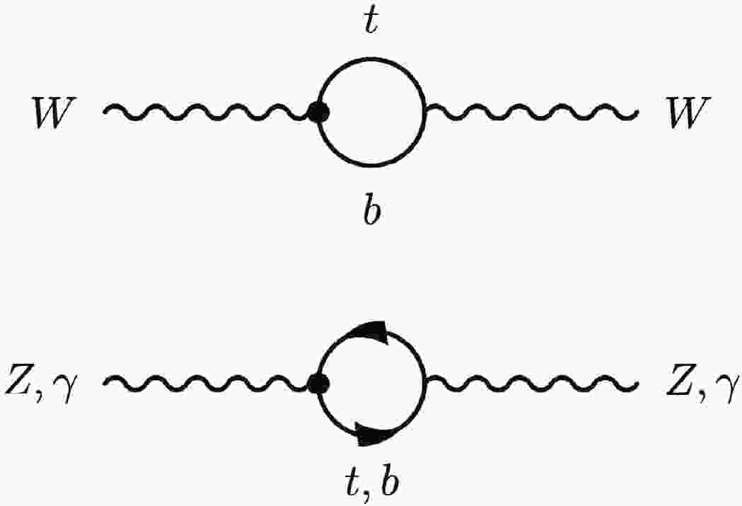
The tree level contributions of the SMEFT dimension-6 operators to the $e^+e^- \to f\bar{f}$ and $e^+e^- \to WW$ processes have been well studied in the past [9–11, 43–46], and we follow these references in our analysis. Here we focus on the one-loop contributions of the 3rd-generation-quark operators in Eq. (2). First, they generate universal contributions to the gauge boson self-energies, as shown in Fig. 1. They have both direct and indirect effects. The indirect effects are the contributions to the measurements of the three input parameters α, $m^2_Z$, and $G_F$. As with the tree level dimension-6 contributions, they change the "inferred SM values" of these parameters. Their effects can be parameterized as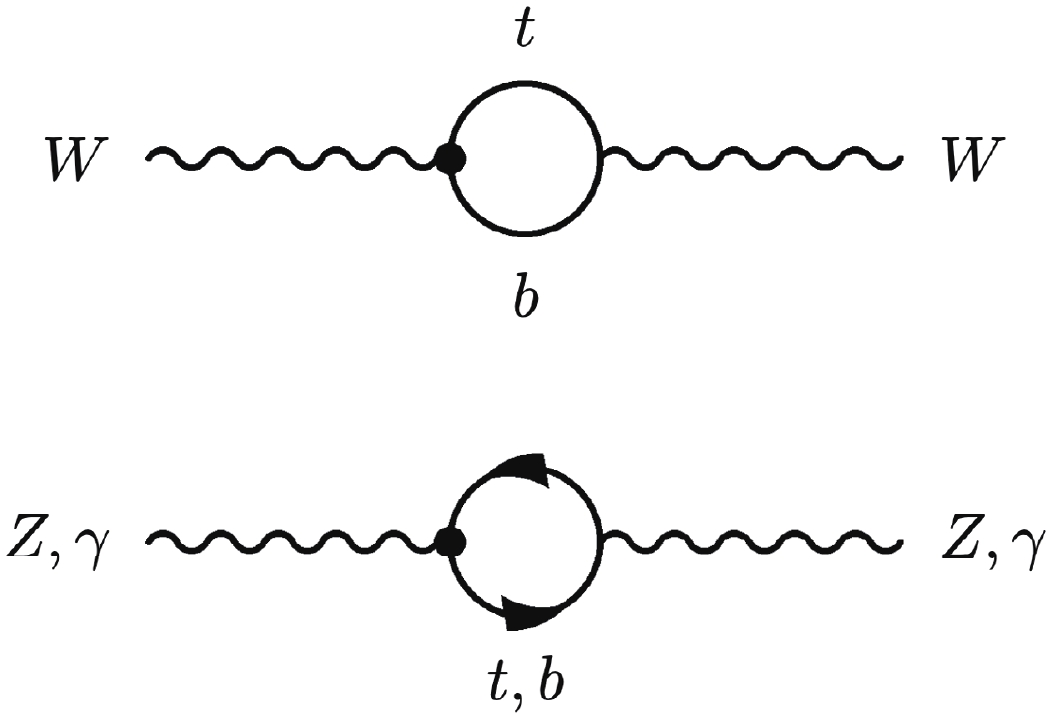

Figure 1.  Gauge boson self-energy correction caused by the operators in Eq. (2). The black dot is the dimension-6 vertex.

where α, $m^{2}_{Z}$, and $G_{F}$ take the values in Eq. (9), $\alpha _{O}$, $m^{2} _{ZO}$, and $G _{FO}$ are the renormalized SM parameters, which are entered into the calculations of EW observables, and $\Pi^{(i)}_{XY}(q^2)$ parameterizes the one-loop corrections to the gauge boson self-energies [47], for which we only consider the contributions from the operators in Eq. (2). Their definitions are shown in Sec. A.3. A renormalized $s^2_W \equiv \sin^2\theta_W$ can be defined as

where $s_{W}^{2}=\dfrac{1}{2}\left(1-\sqrt{1-\dfrac{4\pi\alpha}{\sqrt{2}G_{F}m_{Z}^{2}}}\right)$. The W and Z self-energies also directly enter the observables. The contributions to $e^+e^- \to f\bar{f}$ as well as the W and Z decay rates can be characterized by the tree-level neutral and charged current interactions. At tree level, they are given by (assuming no tree-level contributions from dimension-6 operators)

where $I^{(')}_{3}$and $Q^{(')}$ are the $S U(2)$ and electric charges of the external fermions, respectively, $I_{+}, I_{-}$ are the isospin-raising and isospin-lowering matrices, respectively, and $\alpha _{O}$, $m^{2} _{ZO}$, $G _{FO}$, and $s^{2} _{WO}$ are the renormalized SM parameters in Eqs. (10) and (11). With the direct contributions from the W and Z self-energies, Eq. (12) is modified to

where $m^2_{W*} (q^2)$, $m^2_{Z*} (q^2)$, $Z_{W*} (q^2)$, $Z_{Z*} (q^2)$, $s^2_{W*} (q^2)$, and $e^2_* (q^2)$ generally depend on $q^2$ of the propagators, and their expressions are also listed in Sec. A.3 [48]. In addition to the W and Z self-energies, the 3rd-generation-quark operators also directly modify the $Zb\bar{b}$ vertex^③, as shown in Fig. 2, thus generating non-universal effects. Finally, they also contribute to the processes $e^+e^-\to WW$ and $e^{+}e^{-}\to e^{+}e^{-}$. The calculation of these effects are rather complicated, and we rely on Monte Carlo integration with MadGraph5_aMC@NLO [53]. The method of reweighting [54] is used to generate weighted events. The SM input parameters used in Monte Carlo are the same as those in Eq. (9). We also check that the statistical uncertainties due to simulation sample size are sufficiently small and can be neglected. The numerical results of our calculation can be found in the GitHub repository^④.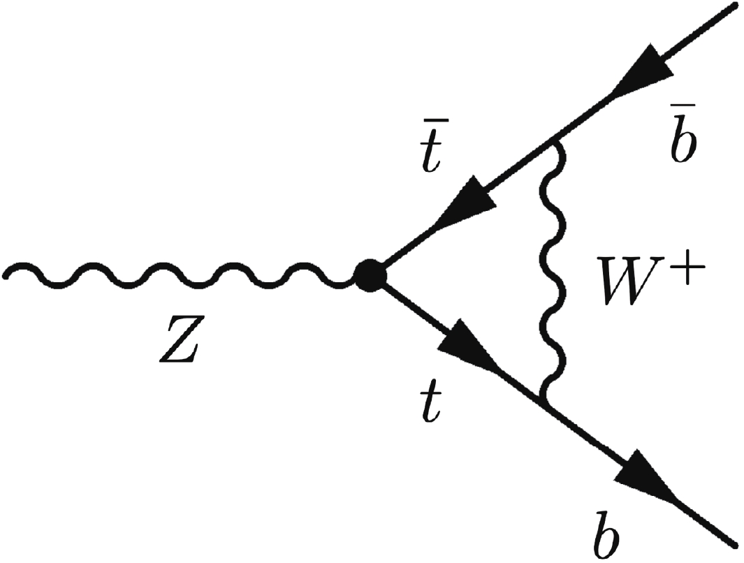

Figure 2.  Diagram of top loop modification to $bb$ production.

The one-loop contributions to EW observables from dimension-6 operators were also recently studied in Refs. [55, 56]. In Ref. [55], the one-loop order QCD and electroweak corrections to the Z and W pole observables are computed under the flavor universality assumption. In contrast, our study focuses on 3rd generation quarks. By also computing the one-loop contributions of the first two generations of quarks and then imposing the flavor universality assumption, we manage to reproduce the results in Ref. [55] on the contributions of $O_{\varphi t}$, $O_{tW}$, and $O_{tB}$ to the $Z\rightarrow bb$ decay width. For $O_{\varphi Q}^{(-)}$, our result turns out to be approximately four times larger than that in Ref. [55], which is likely due to the different choice of cutoff energy. In Ref. [56], the one-loop corrections of flavor non-universal 4-fermion interactions were investigated, which complements our study.

The data used in this study are mainly from the LEP experiment. Data from low energy experiments, such as CHARM [57], CDHS [58], CCFR [59], NuTeV [60], APV [61], QWEAK [62], and PVDIS [63] are also included. These can be divided into the following categories:

● Precision electroweak measurement: We use the Z-pole measurement from the LEP experiment, W mass measurement taken from the combined results of the PDG Group and branching ratio (BR) information from the LEP.

● $e^+ e^- \to f \bar{f}$: Measurements of electron collision to quark and lepton pairs from the LEP experiment are collected. Several observables measured by TRISTAN at 58 GeV are also included.

● $e^+ e^- \to W^+ W^- \to 4f$: The total cross-section and differential cross-section measurements of $e^+ e^- \to W^+ W^- \to 4f$ from the LEP experiment are included in this study.

● Low energy measurement: The neutral-current parameters for ν-hadron and $\nu-e$ processes measured using deep inelastic scattering (DIS) experiments, including CDHS and CHARM in CERN, and CCFR and NuTeV in FermiLab. The parameters for electron scattering are measured using the Cs atomic parity violation (APV) experiment, electron-deuteron DIS (eDIS) experiment PVDIS, and Qweak, which measures the weak charge of protons. Additionally, the cross-section measurement of trident production ($\nu_\mu \gamma^* \rightarrow \nu_\mu \mu^+ \mu^-$) over its SM prediction by CHARM and CDHS is included.

For the data mentioned above, we take the center values, uncertainties, and correlations. The correlations between different categories and experiments are taken as zero. For those with unidentifiable correlations, we make the assumption that they are not correlated with each other. Table 2 shows the varieties of observables included in this study and their references.

	Experiment	Observables	Reference
Low energy	CHARM/CDHS/CCFR/NuTeV/APV/QWEAK/PVDIS	Effective couplings	[42, 64]
Z-pole	LEP/SLC	Total decay width $\Gamma_Z$ Hadronic cross-section $\sigma_{\rm had}$ Ratio of decay width $R_f$ Forward-Backward asymmetry $A_{\rm FB}^f$ Polarized asymmetry $A_f$	[10]
W-pole	LHC/Tevatron/LEP/SLC	Total decay width $\Gamma_W$W branching ratios ${\rm Br}(W\rightarrow l v_l)$Mass of W boson $M_W$	[10, 42]
$ee\rightarrow qq$	LEP/TRISTAN	Hadronic cross-section $\sigma_{\rm had}$Ratio of cross-section $R_f$Forward-Backward asymmetry for b/$c A_{\rm FB}^f$	[65, 66, 67]
$ee \rightarrow ll$	LEP	Cross-section $\sigma_f$Forward-Backward asymmetry $A_{\rm FB}^f$Differential cross-section ${ {\rm d}\sigma_f}/{ {\rm d}{\rm cos}\theta}$	[65]
$ee\rightarrow WW$	LEP	Cross-section $\sigma_{WW}$Differential cross-section ${ {\rm d}\sigma_{WW} }/{ {\rm d}{\rm cos}\theta}$	[65]

Table 2.  Observables used in this study.

Table A1 in the appendix lists the type-I operators that have an impact on the above observables. Besides these, five operators ($Q_{\varphi WB}$, $Q^{ijji}_{ll}$, $Q_{\varphi D}$, $Q^{11(3)}_{\varphi l}$, and $Q^{22(3)}_{\varphi l}$) have an impact on all the obersvables because they affect the electroweak parameters g, $g^{'}$, and v. In the following part, details about several of the categories involved in the experiments will be discussed. These details also affect the generation of Monte Carlo events. Additionally, the uncertainties on SM calculation and experimental measurement will be discussed.

Processes	Observables	Wilson Coefficient
Neutrino DIS and APV	$g _ { L V } ^ { \nu e },g _ { L A } ^ { \nu e }$	$c^{(1)}_{\varphi l},c_{\varphi e},c_{ll},c_{le}$
	$g _ { A V } ^ { e u } + 2g _ { A V } ^ { e d }$$2g _ { A V } ^ { e u } - g _ { A V } ^ { e d }$ $2g _ { V A } ^ { e u } - g _ { V A } ^ { e d }$	$c^{(1)}_{\varphi q}$,$c^{(3)}_{\varphi q},c_{\varphi u}$,$c_{\varphi d}$,$c^{(1)}_{\varphi l}$$c_{\varphi e}$,$c^{(1)}_{lq}$,$c^{(3)}_{lq}$,$c_{lu},c_{ld}$, $c_{qe}$,$c_{eu}$,$c_{ed}$
	$g _ { V A } ^ { e e }$	$c _ { \varphi l } ^ { (1)},c_{\varphi e}, c _ { e e },c _ { l l}$
	$2 \frac{g_{LV}^{\nu_{\mu}\mu,\mathrm{SM}}\delta g_{LV}^{\nu_{\mu}\mu}+g_{LA}^{\nu_{\mu}\mu,\mathrm{SM}}\delta g_{LA}^{\nu_{\mu}\mu}}{\left(g_{LV}^{\nu_{\mu}\mu,\mathrm{SM}} \right)^{2}+\left(g_{LA}^{\nu_{\mu}\mu,\mathrm{SM}} \right)^{2}}$	$c_{\varphi l}^{(1)}$,$c_{\varphi e}$,$c_{le}$, $c_{ll}$
Z-pole	$\Gamma_{Z}$	$c_ { \varphi l } ^ { (1) },c _ {\varphi e },c_ { \varphi q } ^ { (3) },c_ { \varphi q } ^ { (1) },c_{\varphi u},c _ { \varphi d },c_ { \varphi Q} ^ { (+) },c_ { \varphi b }, c_{bB}, c_{bW}$
	$\sigma_{had}$	$c_ { \varphi l } ^ { (1) },c _ { \varphi e },c_ { \varphi q } ^ { (3) },c_ { \varphi q } ^ { (1) },c_{\varphi u},c _ {\varphi d },c_ { \varphi Q} ^ { (+) },c_ { \varphi b }, c_{bB}, c_{bW}$
	$R_{e}$	$c_ { \varphi l } ^ { (1) },c _ { \varphi e },c_ {\varphi q } ^ { (3) },c_ { \varphi q } ^ { (1) },c_ { \varphi u },c_{\varphi d},c_ { \varphi Q} ^ { (+) },c _ {\varphi b }, c_{bB}, c_{bW}$
	$R_{\mu}$	$c_ { \varphi l } ^ { (1) },c _ { \varphi e },c_ { \varphi q } ^ { (3) },c_ { \varphi q } ^ { (1) },c_ { \varphi u },c_{\varphi d},c_ { \varphi Q} ^ { (+) },c _ {\varphi b }, c_{bB}, c_{bW}$
	$R_{\tau}$	$c_ { \varphi l } ^ { (1) },c _ { \varphi e },c_ { \varphi q } ^ { (3) },c_ { \varphi q } ^ { (1) },c_ { \varphi u },c_{\varphi d},c_ { \varphi Q} ^ { (+) },c _ {\varphi b }, c_{bB}, c_{bW}$
	$A^{o,e}_{FB}$	$c _ { \varphi l } ^ { (1) },c_ { \varphi e }$
	$A^{o,\mu}_{FB}$	$c _ { \varphi l } ^ { (1) },c_ { \varphi e }$
	$A^{o,\tau}_{FB}$	$c _ { \varphi l } ^ { (1) },c_ { \varphi e }$
Continued on next page

Table A1.  List of the corresponding coefficients of type I operators that contribute to different observables. Besides these coefficients, there are also four Wilson coefficients that contribute to all observables: $c^{(3)}_{\varphi l}, c^{'}_{ll}, c_{\varphi D}, c_{\varphi WB}$.

Table A1-continued from previous page
Processes	Observables	Wilson coefficient
	$R_{b}$	$c_ { \varphi q } ^ { (3) },c_ { \varphi q } ^ { (1) },c _ { \varphi u },c _ { \varphi d},c_ { \varphi Q} ^ { (+) },c_{\varphi b}, c_{bB}, c_{bW}$
	$R_{c}$	$c_ { \varphi q } ^ { (3) },c_ { \varphi q } ^ { (1) },c _ { \varphi u },c _ { \varphi d},c_ { \varphi Q} ^ { (+) },c_{\varphi b}, c_{bB}, c_{bW}$
	$A^{b}_{FB}$	$c_ { \varphi l } ^ { (1) },c_ { \varphi e },c_ {\varphi Q } ^ { (+) },c _ { \varphi b }, c_{bB}, c_{bW}$
	$A^{c}_{FB}$	$c _ { \varphi l } ^ { (1) },c_ { \varphi e },c_ { \varphi q } ^ { (1) },c _ { \varphi q } ^ { (3) },c _ { \varphi u },$
	$A_{e}$	$c _ { \varphi l } ^ { (1) },c_ { \varphi e }$
	$A_{\mu}$	$c _ { \varphi l } ^ { (1) },c_ { \varphi e }$
	$A_{\tau}$	$c _ { \varphi l } ^ { (1) },c_ { \varphi e }$
	$A_{b}$	$c_ { \varphi Q } ^ { (+) },c _ { \varphi b }, c_{bB}, c_{bW}$
	$A_{c}$	$c_ { \varphi q } ^ { (1) },c_ { \varphi q } ^ { (3) },c _ { \varphi u }$
	$A_{s}$	$c_ { \varphi q } ^ { (1) },c_ { \varphi q } ^ { (3) },c _ { \varphi d }$
W-pole	$M_{W}$
	$Br(W\to e\nu_{e})$ $Br(W\to\mu\nu_{\mu})$ $Br(W \to\tau\nu_{\tau})$$\Gamma_{W}$	$c _ { \varphi q } ^ { (3) }$
$ee\to q\bar{q}$	$\sigma_{eeqq}$	$c _ { \varphi l } ^ { (1) }$,$c _ { \varphi e }$,$c _ { \varphi q } ^ { (3) }$,$c _ {\varphi q } ^ { (1) }$,$c _ { \varphi u }$,$c _ { \varphi d }$,$c _ { \varphi Q} ^ { (+) }$,$c_ { \varphi b }$,$c _ { l q } ^ { (1) }$,$c _ { l q } ^ { (3) }$, $c_{ l u }$,$c _ { l d }$,$c_ { l Q } ^ { (+) }$,$c _ { l b}$,$c _{ q e }$,$c_{eu}$,$c_ { e d }$,$c _ { eQ}$,$c _ { e b}, c_{bB}, c_{bW}$
$ee\to b\bar{b}$	$\sigma_{eebb}$	$c _ { \varphi l } ^ { (1) },c _ { \varphi e },c _ { \varphi Q } ^ { (+) },c _ { \varphi b },c_ { l Q}^ { (+) },c _ { l b},c _ { eQ},c_ { e b}, c_{bB}, c_{bW}$
$ee\to c\bar{c}$	$\sigma_{eecc}$	$c _ { \varphi l } ^ { (1)}$,$c _ { \varphi e }$,$c _ { \varphi q } ^ { (1) }$,$c _ { \varphi q } ^ { (3) }$,$c_ { \varphi u }$,$c_{ l q } ^ { (1) }$,$c_ { l q } ^ { (3) }$,$c _ { l u }$,$c_ { q e }$,$c_ { e u }$
$ee\to \mu^{+}\mu^{-}$	$\sigma_{ee\mu\mu}$	$c_ { \varphi l } ^ {(1) }$,$c_ { \varphi e }$,$c_ { ll}$,$c _ { l e }$,$c _ { e e }$
$ee\to\tau^{+}\tau^{-}$	$\sigma_{ee\tau\tau}$	$c_ { \varphi l } ^ { (1) }$,$c_ { \varphi e }$,$c_ { ll}$,$c _ { l e }$,$c _ { e e }$
$ee\to e^{+}e^{-}$	$\sigma_{eeee}$	$c_ { \varphi l } ^ { (1)}$,$c_ { \varphi e }$,$c_ { ll}$,$c _ { l e }$,$c _ { e e }$
$ee\to W^{+}W^{-}$	$\sigma_{eeww}$	$c _ { \varphi l } ^ { (1)}$,$c_ { \varphi e }$,$c _ { W }$

The theoretical predictions of Z pole and W pole observables are taken from Table 10.5 of [42] and Table 2 of [11]. The theoretical errors on the Z and W pole observables and low energy couplings, except for $m_{W}$, are ignored (the theoretical prediction error om $m_{W}$ is 0.004 GeV [42, 68]).

The main Feynman diagram of $e^+ e^- \rightarrow f \bar{f}$ contains an s-channel photon and Z annihilation (Fig. 3(a)). However, there is an additional t-channel photon and Z exchange in the $e^+ e^- \rightarrow e^+ e^-$ process (Fig. 3(b)), which have a small contribution at the Z-pole. We make the assumption of zero electron and muon mass in our model. As a result, there is only a negligible difference between the contribution of new operators to the observables of the $e^+ e^- \rightarrow e^+ e^-$ and $e^+ e^- \rightarrow \mu^+ \mu^-$ processes, and we take the result of $e^+ e^- \rightarrow \mu^+ \mu^-$ as that of $e^+ e^- \rightarrow e^+ e^-$ at the Z-pole. At other energies, both t-channel and s-channel production of $e^+ e^- \rightarrow e^+ e^-$ are considered.

Figure 3.  Feynman diagrams for the $e^+ e^- \to$$f \bar{f}$ process at the Born level.

For quark pair production, the decay of quarks is not considered. Additional observables in the low energy region for b and c quark production are included, which helps us obtain a better constraint on the 3rd-generation-quark operators.

For fermion-pair production, especially at energies above Z resonance, the QED radiative corrections are very large. This is caused by the initial-state radiation of photons, which lowers the center-of-mass energy, $\sqrt{s}$, to a value of $\sqrt{s'}$. In the LEP experiment, the measurement is performed using events with a small amount of initial state radiation, that is, large $\sqrt{s/s'}$. Therefore, in Monte Carlo integration, initial-state radiation is not considered.

● In the $e^{+}e^{-}\to f\bar{f}$($f=\mu, \tau, q$) processes, the experimental values of cross-sections (in pb) and forward-backward asymmetries are reported in Table 3.4 of [65]. The theoretical prediction uncertainties on $\sigma(q\bar{q}), \sigma(\mu^{+}\mu^{-})$, and $\sigma(\tau^{+}\tau^{-})$ and leptonic forward-backward asymmetries are $0.26$%, $0.4$%, $0.4$%, and $0.4$%, respectively [65, 69]. Their theoretical prediction uncertainties can be neglected because their experimental uncertainties are at least four times larger.

● The experimental and theoretical values of the $e^{+}e^{-}\to\mu^{+}\mu^{-}$and $e^{+}e^{-}\to\tau^{+}\tau^{-}$ differential cross-sections are reported in Tables 3.8 and 3.9 of [65]. In the processes $e^{+}e^{-}\to\mu^{+}\mu^{-}$ and $e^{+}e^{-}\to\tau^{+}\tau^{-}$, we assume that the theoretical uncertainty on the differential distribution is 0.4%, which can be neglected compared with experimental values.

● The experimental and theoretical values of the $e^{+}e^{-}\to e^{+}e^{-}$ differential cross-section are reported in Tables 3.11 and 3.12 of [65]. The theoretical uncertainty on large-angle Bhabha scattering for $\sqrt{s}$ ranging from 189 to 207 GeV is approximately 0.5% [69, 70]. The theoretical uncertainty on the differential distribution is also taken as 0.5%.

● For the process $e^{+}e^{-}\to q\bar{q}$ at $\sqrt{s}=58$ GeV, Table 8 in [71] show the experimental values for $R_{b}$ and $R_{c}$, which are the bottom and charm quark pair production cross-section ratios to the total hadronic cross-section. In [72], their theoretical uncertainties are estimated as 1% and can be ignored.

● For the process $e^{+}e^{-}\to q\bar{q}$ at $\sqrt{s}$ ranging from 189 to 207 GeV, Tables 8.9 and 8.10 in [66] show the experimental values for $R_{b}$ and $R_{c}$ without theoretical uncertainties. We assume the theoretical uncertainties are negligible.

Boson-pair production is also very important in LEP experiments. In our study, the $e^+ e^- \rightarrow W^+ W^-$ process is included. There are three main Feynman diagrams for this process, shown in Fig. 4, which are known as CC03 (Charged Current).

Figure 4.  Main Feynman diagrams for $e^+ e^- \rightarrow W^+ W^-$ at the Born level.

Figure 13.  (color online) Comparison of the current precision of EW observables and the projections for CEPC and FCC-ee.

The W boson will decay into a quark-antiquark pair or lepton-neutrino pair. The BR of hadronic decay is approximately 67%, and that of leptonic decay is approximately 33%. $WW$ events are classified into fully hadronic, semi-leptonic, and fully leptonic events. In the Monte Carlo simulation of the total cross-section of $WW$ production, we ignore the decay of W bosons and only produce events that take the W pair as the final state for convenience. The angular distribution of $WW$ events (${\rm d}\sigma_{WW}/{\rm dcos}\theta_{W^-}$) is also included in this study, where $\theta_{W^-}$ is the polar angle between $W^-$ and the $e^-$ beam direction. In the differential cross-section measurement, the decay of $WW$ is selected as $q\bar{q}e\nu$ and $q\bar{q}\mu\nu$ because these two types of leptonic decays provide the charge tag and a clean background compared with the τ channel. There is a constraint on the experiment that the charged lepton should be $20^\circ$ from the beam, $|\theta_l|>20^\circ$. This angular cut brings about a 93% cut efficiency in the experiment, [65] which matches our Monte Carlo simulation with the SM model. This angular requirement corresponds to the experimental acceptance of the four LEP experiments and also greatly reduces the difference between the full 4f cross-section and the CC03 cross-section by reducing the contribution of t-channel diagrams in the $q\bar{q}e\nu$ final state. (As stated in the LEP result, the difference of the 4f and CC03 cross-sections decreased from 24.0% to approximately 3.5% with the angular cut.) However, its effect is no longer the same for the contribution from new physics. Based on our simulation, the angular cut efficiency of some operators is shown in Fig. 5. The cut efficiency of operators that contribute to the differential cross-section at different energies can be found in the appendix. As a result, the decay of W cannot be ignored in the simulation of W angular distribution. Taking the four fermions as the final state, the process $e^+ e^- \rightarrow W^+ W^- \rightarrow q \bar{q} l \nu$ would be a subset of the process $e^+ e^- \rightarrow q \bar{q} l \nu$. If we simulate the process $e^+ e^- \rightarrow W^+ W^- \rightarrow q \bar{q} l \nu$ and allow the W boson to be off-shell, the gauge invariance would be broken. However, simulating the process $e^+ e^- \rightarrow q \bar{q} l \nu$ would bring about an additional Feynman diagram. Finally, we decided to simulate the process $e^+ e^- \rightarrow W^+ W^- \rightarrow q \bar{q} l \nu$ using MadSpin [73] to place W on shell decay to guarantee gauge invariance.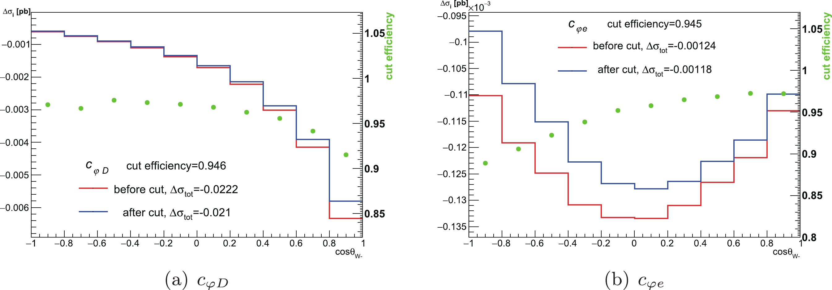

Figure 5.  (color online) Impact of the 20 degree angular cut on the operators $c_{\varphi D}$ and $c_{\varphi e}$ at 183 GeV. The red line shows the differential cross-section of the operators before the angular cut, and the blue line shows the differential cross-section after the cut. The overall cut efficiency is given by the total cross-section after the cut divided by that before the cut.

In [74, 75], the theoretical uncertainties on the $W^{-}$ angular distribution are approximately $0.5$% when $\sqrt{s}$ ranges from 180 to 210 GeV. Because the experimental precision of $W^{-}$ differential angular cross-section are at least seven times larger than the theoretical ones, we can neglect the theoretical prediction uncertainties on $W^{-}$ differential angular cross-section. Although the theoretical uncertainties on the total cross-section of W pair production are also approximately $0.5$% for $\sqrt{s}$ ranging from 180 to 210 GeV, they are non-negligible because the experimental uncertainties are comparable with the theoretical values.

The SMEFT Wilson coefficients are estimated using the least squares method under the assumption of Gaussian errors. The $\chi^2$ function is constructed as

where $\vec{y}$ is the vector of the difference between the experimental result and SM prediction of the observables, A is the contribution matrix ($A_{ij}$ is the i-th operator contribution to j-th observables), $\vec{c}$ is the vector of the Wilson coefficient, and V is the covariance matrix of the observables.

By letting $\nabla\chi^2=0$, we can obtain the least square estimator $\hat{\vec{c}}\;$ that minimizes $\chi^2$ and its covariance matrix U,

The element of the covariance matrix, $U_{ij}$, represents the covariance of the estimators $\hat{c_i}$ and $\hat{c_j}$. The one-sigma bound of $c_i$ can be obtained from the diagonal element of this matrix.

We apply the aforementioned fit strategy to obtain the constraints of the EFT operator coefficients. Two types of bounds are shown. The first is the marginalized bound, derived allowing all operator coefficients to float. When conducting this type of fit, the correlations between the coefficients also contain useful information. The second is the individual bound, which is obtained by considering only one operator coefficient at a time while fixing all others to zero. In the following results, all the bounds are given in the 68% confidence level (CL). The new physics scale Λ of the Wilson coefficients $\dfrac{c_i}{\Lambda^2}$ is fixed to be 1 TeV throughout this section.

We consider a total of 33 operators listed in Section II, which are constrained by the measurements in Sec. III. As mentioned in Sec. II, we trade $\dfrac{c_{\varphi D}}{\Lambda^{2}}Q_{\varphi D}$ and $\dfrac{c_{\varphi WB}}{\Lambda^{2}}Q_{\varphi WB}$ in the Warsaw basis for $\dfrac{c_{D\varphi B}}{\Lambda^{2}}{\rm i}D^{\mu}\varphi^{\dagger}D^{\nu}\varphi B_{\mu\nu}$ and $\dfrac{c_{D\varphi W}}{\Lambda^{2}}{\rm i}D^{\mu}\varphi^{\dagger}\sigma_{a}\varphi W^{a}_{\mu\nu}$ to disentangle several large correlations, whereas the other operators in the Warsaw basis remain unchanged. Our main results are presented in Fig. 6 in terms of the one-sigma (corresponding to a 68% confidence level (CL)) bounds of the Wilson coefficients. To understand the impact of the 3rd generation quark operators, we also consider two additional scenarios for comparison: The first considers only tree-level contributions from dimension-6 operators, whereas the second also includes the loop contributions of the bottom-quark operators (that is, excluding $Q^{(-)}_{\varphi Q}$, $Q_{\varphi t}$, $Q_{tW}$, and $Q_{tB}$). The correlations between the coefficients are shown in Fig. 7 for the tree-level-only scenario and Fig. 8 for the full scenario. The numerical results can be found in Table A2 of the appendix, along with the Fisher information matrix for the full scenario.

Figure 6.  (color online) 68% CL bounds of operator coefficients in the modified Warsaw basis for three different scenarios. (blue) Tree-level contribution only. (green) Tree-level contribution and loop contributions from the bottom-quark operators. (red) Tree-level contribution and the loop contributions of all third-generation-quark operators listed in Sec. II. The dark red bar is the individual bound in this scenario. See Table A2 in the appendix for the best-fitted central values. The value of Λ is set to 1 TeV for all coefficients.

Figure 7.  (color online) Correlation matrix between operator Wilson coefficients in the modified Warsaw basis. Only the tree-level contribution of these operators is considered.

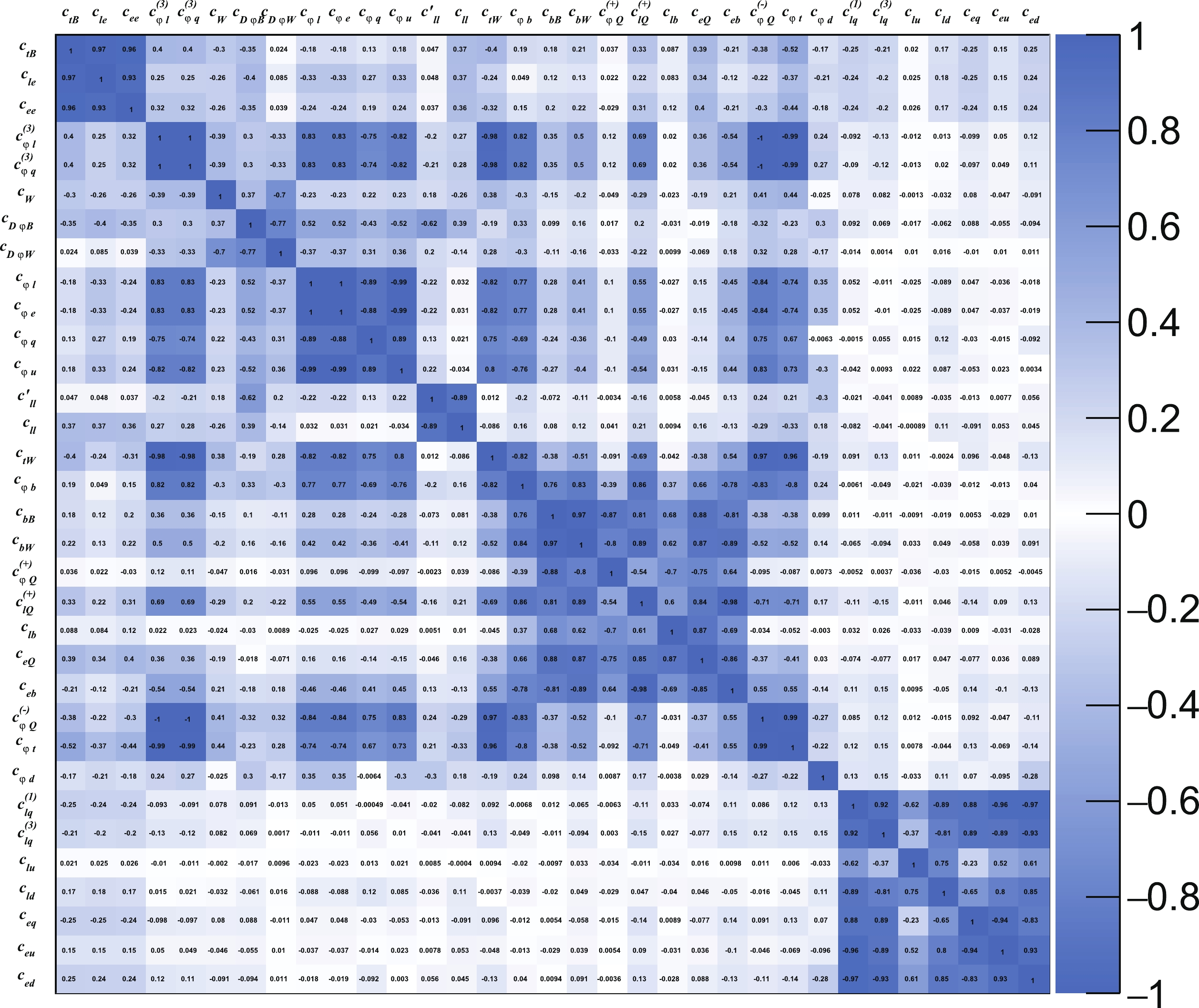
Figure 8.  (color online) Correlation matrix between operator Wilson coefficients in the modified Warsaw basis. The top and bottom loop contributions are considered in addition to the tree-level contribution.

Operators	Marginalized, tree-only	Marginalized, b loop considered	Marginalized, t/b loop considered	Individual, t/b loop considered
$c_{tB}$	−	−	$30 \pm 35$	$-0.13 \pm 0.18$
$c_{le}$	$0.0019 \pm 0.018$	$0.0014 \pm 0.018$	$0.036 \pm 0.036$	$-0.0015 \pm 0.016$
$c_{ee}$	$-0.019 \pm 0.014$	$-0.019 \pm 0.014$	$-0.0082 \pm 0.018$	$-0.012 \pm 0.012$
$c_{\varphi l}^{(3)}$	$-0.023 \pm 0.023$	$-0.027 \pm 0.018$	$-0.42 \pm 2$	$-0.0036 \pm 0.0033$
$c_{\varphi q}^{(3)}$	$-0.079 \pm 0.07$	$-0.11 \pm 0.074$	$-0.47 \pm 2$	$0.0025 \pm 0.0076$
$c_{W}$	$-7.9 \pm 5.1$	$-1.8 \pm 3.7$	$-4.5 \pm 4.5$	$0.41 \pm 0.37$
$c_{D\varphi B}$	$-13 \pm 10$	$-7.9 \pm 11$	$-12 \pm 17$	$-0.2 \pm 1.9$
$c_{D\varphi W}$	$35 \pm 21$	$12 \pm 17$	$23 \pm 20$	$0.82 \pm 1.1$
$c_{\varphi l}$	$0.024 \pm 0.013$	$0.021 \pm 0.013$	$-0.26 \pm 0.67$	$0.0014 \pm 0.0042$
$c_{\varphi e}$	$0.0051 \pm 0.014$	$-2.5e-05 \pm 0.013$	$-0.57 \pm 1.3$	$-0.0018 \pm 0.0054$
$c_{\varphi q}$	$-0.042 \pm 0.13$	$-0.053 \pm 0.14$	$0.085 \pm 0.28$	$-0.015 \pm 0.014$
$c_{\varphi u}$	$0.086 \pm 0.17$	$0.11 \pm 0.17$	$0.49 \pm 0.91$	$-0.011 \pm 0.021$
$c'_{ll}$	$-0.043 \pm 0.03$	$-0.055 \pm 0.029$	$-0.069 \pm 0.094$	$0.0035 \pm 0.0051$
$c_{ll}$	$0.054 \pm 0.033$	$0.066 \pm 0.031$	$0.1 \pm 0.093$	$0.0037 \pm 0.011$
$c_{tW}$	−	−	$4.2 \pm 27$	$-0.3 \pm 0.22$
$c_{\varphi b}$	$-0.34 \pm 0.62$	$-0.27 \pm 0.63$	$-12 \pm 14$	$-0.17 \pm 0.11$
$c_{bB}$	$10 \pm 15$	$9.2 \pm 14$	$12 \pm 18$	$0.25 \pm 0.23$
$c_{bW}$	$16 \pm 27$	$9.7 \pm 25$	$17 \pm 32$	$0.1 \pm 0.13$
$c_{\varphi Q}^{(+)}$	$-3.5 \pm 5.4$	$-2.3 \pm 5$	$-6.1 \pm 5.5$	$0.017 \pm 0.02$
$c_{lQ}^{(+)}$	$-1.5 \pm 2.1$	$-2 \pm 2.4$	$-4.7 \pm 5.5$	$-0.048 \pm 0.042$
$c_{lb}$	$1.2 \pm 2.3$	$1.4 \pm 2.5$	$-1.2 \pm 5.9$	$0.0074 \pm 0.23$
$c_{eQ}$	$0.64 \pm 1.8$	$0.56 \pm 1.8$	$-1.5 \pm 4.8$	$0.035 \pm 0.11$
$c_{eb}$	$3.6 \pm 5$	$5.1 \pm 5.6$	$11 \pm 12$	$-0.1 \pm 0.1$
$c_{\varphi Q}^{(-)}$	−	−	$31 \pm 2.7e+02$	$-0.043 \pm 0.14$
$c_{\varphi t}$	−	−	$3.8 \pm 1.9e+02$	$0.011 \pm 0.12$
$c_{\varphi d}$	$-0.7 \pm 0.8$	$-0.92 \pm 0.86$	$-0.69 \pm 0.99$	$-0.038 \pm 0.028$
$c_{lq}^{(1)}$	$2.3 \pm 1.2$	$2.7 \pm 1.2$	$2.6 \pm 1.2$	$0.014 \pm 0.014$
$c_{lq}^{(3)}$	$0.74 \pm 0.43$	$0.88 \pm 0.43$	$0.84 \pm 0.44$	$0.029 \pm 0.018$
$c_{lu}$	$-1.1 \pm 0.83$	$-1.3 \pm 0.82$	$-1.3 \pm 0.83$	$0.017 \pm 0.026$
$c_{ld}$	$-4.8 \pm 2.4$	$-5.8 \pm 2.4$	$-5.2 \pm 2.4$	$0.042 \pm 0.03$
$c_{eq}$	$2.6 \pm 1.6$	$3 \pm 1.6$	$2.8 \pm 1.6$	$-0.019 \pm 0.014$
$c_{eu}$	$-2.2 \pm 1.1$	$-2.6 \pm 1.1$	$-2.4 \pm 1.1$	$-0.039 \pm 0.023$
$c_{ed}$	$-3.6 \pm 2.1$	$-4.2 \pm 2$	$-4.1 \pm 2.1$	$-0.022 \pm 0.029$

Table A2.  Numerical fit results of the operator coefficients in the modified Warsaw basis for three different scenarios. The error bound is given in the 68% CL.

Overall, our results demonstrate the relevance of 3rd generation quarks in electroweak measurements. The coefficients of the four top operators $Q^{(-)}_{\varphi Q}$, $Q_{\varphi t}$, $Q_{tW}$, and $Q_{tB}$ are constrained in the range of $0.1$ to $1$ for the individual fit, despite the fact that their contributions only enter at the one-loop order. Assuming an order-one coupling, this corresponds to a new physics scale of a few TeVs. After comparing these results with those in Ref. [25], which uses LHC data to probe these four top operators, it is found that the electroweak data have greater constraining power on $Q^{(-)}_{\varphi Q}$ and $Q_{\varphi t}$, whose advantage is estimated to be of the order of 10. Conversely, for $Q_{tW}$ and $Q_{tB}$, the LHC data are more powerful. Their 95% CL individual bounds are listed in Table 3 for comparison.

	$c_{\varphi t}$	$c_{\varphi Q}^{(-)}$	$c_{tW}$	$c_{tB}$
Electroweak	0.286	0.336	0.822	0.592
LHC data	2.275	1.22	0.06	0.145

Table 3.  95% CL individual bounds of top quark operator coefficients using different sets of observables.The electroweak results are from this study, whereas the LHC data are the results in [26].

In a global fit, however, the marginalized bounds of the top-quark operator coefficients become significantly looser, and some of them possibly exceed the range of EFT validity. This is not surprising because the introduction of additional degrees of freedom tends to bring additional flat directions, making the fit difficult to converge. This can also be verified by comparing the correlations in Fig. 7 and Fig. 8; the increase in correlation is visible in the latter. The inclusion of top operators also significantly degrades the reaches of several other operator coefficients. Among them, the most notable are the leptonic operators $c_{l e}$, $c_{e e}$, $c^{(3)}_{\varphi l}$, $c_{\varphi l}$, and $c_{\varphi e}$ (as well as $c^{(3)}_{\varphi q}$), which were previously well constrained and are thus most sensitive to additional degrees of freedom. Note that $c_{l e}$and $c_{e e}$ contribute directly to 4-lepton processes, and their contributions can be distinguished from those with a gauge boson propagator by measuring the processes at several different energies. On the other hand, when only the loop contributions of the bottom-quark operators are included (green bar), the overall reach of the global fit is not significantly degraded compared with that of the tree-level fit, and the reach on some of the operator coefficients are even improved. This is because these operators already contribute at the tree level; hence, the number of operators is not increased, whereas their dependence on the observables changes with the inclusion of loop effects.

It should be noted that, as pointed out in Section II, the effects of the two bottom-quark dipole operators $Q_{bW}$ and $Q_{bB}$ are non-negligible and should be included in the fit. Even at the tree level, this introduces large flat directions with the operators $Q^{(+)}_{\varphi Q}$ and $Q_{\varphi b}$because the four operators are mainly constrained by only two observables, $R_b$ and $A_b \,(A^b_{\rm FB})$. Among them, we observe particular strong correlations among $Q_{bW}$, $Q_{bB}$, and $Q^{(+)}_{\varphi Q}$ ($>0.98$), whereas their correlations with $Q_{\varphi b}$ are relatively smaller ($<0.9$). This is because the former three operators mainly contribute to $R_b$, while $Q_{\varphi b}$ modifies the $Zb_R\bar{b}_R$ coupling and is more sensitive to asymmetry (see, for example, Ref. [76]).

Additional results are also provided in Table A2 in the appendix, which shows both the marginalized bound with central values and individual bounds. Figure A1 shows the impact of different sets of measurements on the Wilson coefficients, which is given by Fisher information.

Figure A1.  (color online) Impact of different sets of measurements on the Wilson coefficients in the Warsaw basis, measured using Fisher information. The larger the number is, the bigger impact of the set have on the constraints of Wilson coefficients.

In addition to the general global-fitting framework, we also consider a special case denoted here as the "$S\,T \, t\,b$" scenario, where we assume that all new physics effects, apart from those in Eq. (2), can be parameterized by the two oblique parameters S and T [47]. This scenario is motivated by a large class of models with top/bottom partners, which generally mixes with 3rd generation quarks and can also contribute to oblique parameters at the one-loop order. For convenience, we work with the modified parameters $\hat{S}$ and $\hat{T}$ [77], which are related to the original parameters via

$\hat{S}$and $\hat{T}$ are defined based on [78]. The measurements considered are still the same as in Sec. IV.B.

For comparison, we first consider the two-parameter fit of $\hat{S}$ and $\hat{T}$. Their 68% CL preferred region and correlation are shown in Fig. 9. The numerical results of the individual and marginalized bound are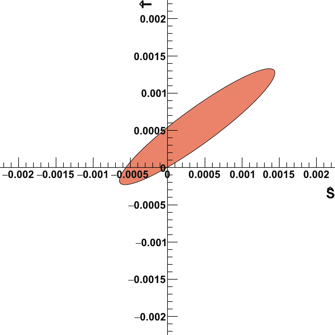

Figure 9.  (color online) 68% CL preferred region of $\hat{S}$ and $\hat{T}$.

and

with the correlation

These results are comparable with those in Ref. [79], which uses the same set of measurements as we do.

With the inclusion of the 3rd-generation quark operators, we perform a 10-parameter fit, and the results are presented in Fig. 10. It should be noted that part of the loop contributions of the 3rd-generation quark operators is universal and can be absorbed in the original definition of the S and T parameters. Here, by $\hat{S}, \hat{T}$, we simply denote the contributions of the corresponding tree-level operators. From Fig. 10, we observe a significantly better reach on the top quark operators compared with the general case in Sec. IV.B. However, the constraining power to the $\hat{S}$ and $\hat{T}$ parameters with the electroweak data is significantly reduced from the 2-parameter case, as expected.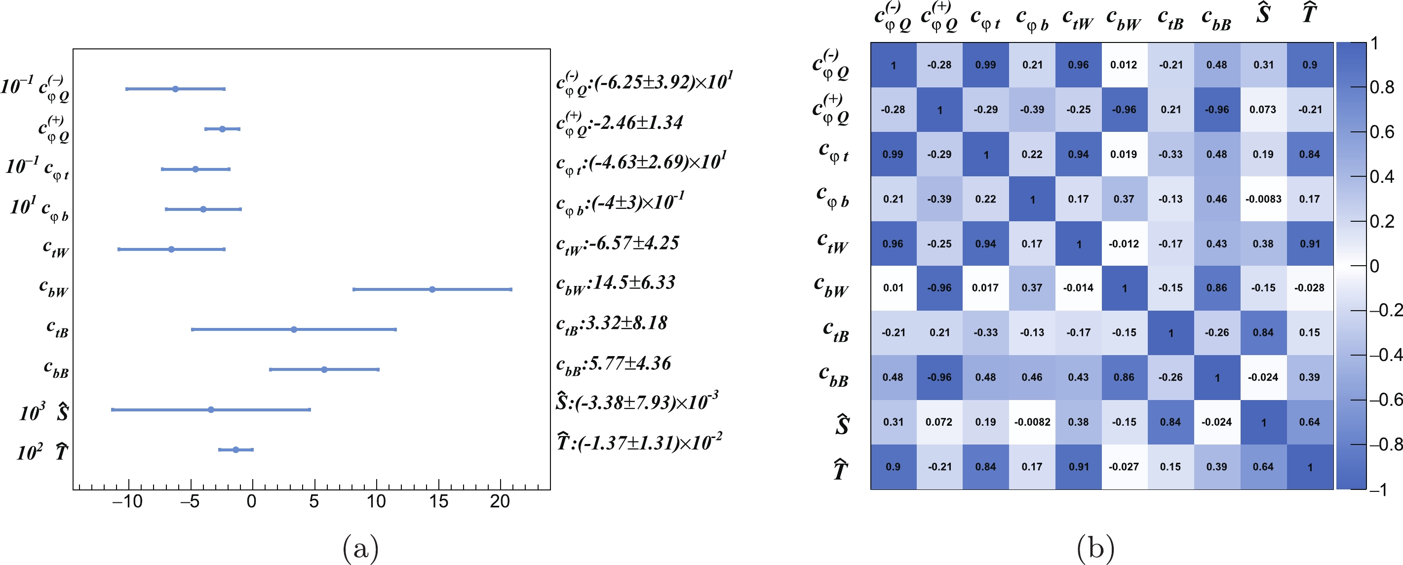

Figure 10.  (color online) Fit results ((left) 68% CL marginalized bound, (right) correlation matrix) of the $\hat{S}$ and $\hat{T}$ parameters and the eight operator coefficients in Eq. (2).

One could also consider a more general set of universal corrections [78] (in addtion to the 3rd generation quark operators), which also requires additional measurements. For instance, the W and Y parameters are strongly constrained by the high energy Drell-Yan measurement at the LHC [80]. A detailed analysis in this direction is left for future studies.

The CDF experiment recently announced their new W mass measurement [40], which deviated from the SM prediction by seven standard deviations. This measurement will greatly affect the fit results. Therefore, in this section, the fit results with this new measured W mass are shown in contrast with those using the previously measured value. Fig. 11 shows the individual bound changes with the new measurement.

Figure 11.  (color online) Individual bounds of operator coefficients in the modified Warsaw basis with the previous (blue) and new (red) W mass measurement. Here, both the tree-level contribution and the loop contributions of all third-generation-quark operators are considered.

With the new CDF W-mass measurement, the results of the $\hat{S}$-$\hat{T}$ two-parameter fit are

and

For the "$S\,T \, t\,b$" scenario, Fig. 12 shows the marginalized bound with the new W mass measurement. The impact of the shifted W mass value is greatly absorbed by the 3rd-generation-quark operators.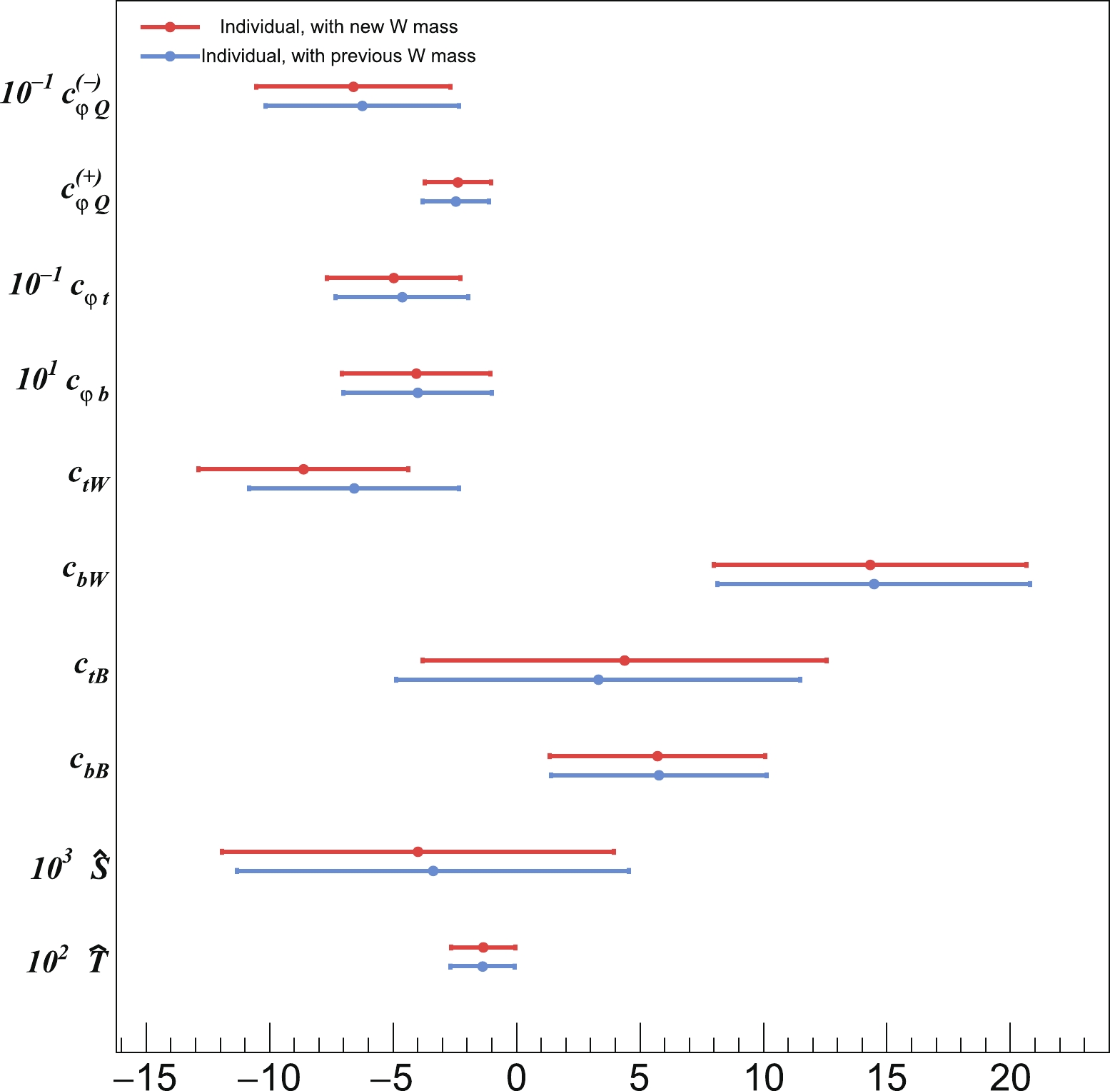

Figure 12.  (color online) 68% CL marginalized bound of operator coefficients in the "$S\,T \, t\,b$" scenario with the new W mass measurement (red) and previous value (blue).

There are several papers [81–90] that also study the impact of the new $m_W$ measurement on new physics scenarios, especially the SMEFT fit and oblique parameters. These results are generally in good agreement with our results.

Recently, there have been several proposals on the construction of future colliders that can reach higher luminosities and energies and will thus significantly increase the precision of electroweak measurements. It is interesting to see how the improvement of measurement affects the constraints on these EFT operators. As a result, the projections of electroweak observables from FCC-ee and CEPC are collected to conduct a chi-square fit. For the other two future collider proposals, the ILC and CLIC, because their Giga-Z proposals are still under discussion and currently there is little information on their expected performance for electroweak observables, they are not included in this study.

In Table 4, we show a comparison of the current precision of electroweak observables and the projections for the CEPC and FCC. Because both experiments are designed to be tera-Z factories, the projections of observables at the Z-pole are taken as a common value. For the CEPC, the projections of luminosity at the WW threshold and 240 GeV are taken from Ref. [91]. For the FCC-ee, the predictions are taken from Ref. [92]. The projections of the constraints on the EFT operators involved in this study are shown in Fig. 13. In general, the future collider will greatly improve the constraining power on these EFT operators; most of the coefficients will obtain at least 10 times better constraints, both on individual and marginalized bounds. Though 3rd-generation quark operators can only be probed at loop level in current projections, they still have significantly better constraints. For several operators, such as $Q_W$ and $Q_{eq}$, their constraints experience relatively small improvement because their constraints mainly originate from the $e^+e^-\to W^+W^-$ process or low energy coupling measurements, which lack the projection of their precision for future colliders. However, it is believed that they can also benefit from the high precision measurements of future colliders. Finally, a high-energy lepton collider running at and above the top threshold will be able to measure the $e^+e^-\to t\bar{t}$ process to an unprecedented precision, providing the ultimate probe for 3rd-generation quark operators [15, 20, 25]. The interplay between the top, Higgs, and EW measurements in probing 3rd-generation quark operators is an important topic for future collider studies; however, this is beyond the scope of our current study.

Observables	SM	Current precision	CEPC	FCC-ee
$\Gamma_Z$	2.4942 G${\rm e}{\rm V}$	2.3 M${\rm e}{\rm V}$	0.1 M${\rm e}{\rm V}$	0.1 M${\rm e}{\rm V}$
$\sigma_{\rm had}$	41.481 nb	0.037 nb	0.004 nb	0.004 nb
$R_e$	20.737	0.05	0.001	0.001
$R_\mu$	20.737	0.033	0.001	0.001
$R_\tau$	20.782	0.045	0.001	0.001
$R_b$	0.21582	0.00066	0.00006	0.00006
$R_c$	0.17221	0.003	0.00026	0.00026
$A_{\rm FB}^b$	0.103	0.0003	0.0003	0.0003
$A_\tau$	0.1472	0.00216	0.0002	0.0002
$M_W$	80.379 G${\rm e}{\rm V}$	12 M${\rm e}{\rm V}$	1 M${\rm e}{\rm V}$	0.5M${\rm e}{\rm V}$
$\Gamma_W$	2.085 G${\rm e}{\rm V}$	42 M${\rm e}{\rm V}$	2.8 M${\rm e}{\rm V}$	1.2 M${\rm e}{\rm V}$
$\sigma_{ee\to ff}^{160\;{\rm GeV} }$	−	−	$\sqrt{\dfrac{\sigma_{\rm SM}}{2.6ab^{-1}}}$	$\sqrt{\dfrac{\sigma_{\rm SM}}{12ab^{-1}}}$
$\sigma_{ee\to ff}^{240\;{\rm GeV} }$	−	−	$\sqrt{\dfrac{\sigma_{\rm SM}}{5.6ab^{-1}}}$	$\sqrt{\dfrac{\sigma_{\rm SM}}{5ab^{-1}}}$
$\sigma_{ee\to \mu\mu/\tau\tau, \rm differential}^{240\;{\rm GeV} }$	−	−	$\sqrt{\dfrac{\sigma_{\rm SM}}{5.6ab^{-1}}}$	$\sqrt{\dfrac{\sigma_{\rm SM}}{5ab^{-1}}}$

Table 4.  Comparison of the projections of electroweak observables for the CEPC [91] and FCC-ee [92].

Precision measurements of electroweak processes offer important probes for physics beyond the SM. Many SMEFT analyses of electroweak measurements focus on the tree-level contributions of dimension-6 operators. However, given the outstanding precision of these measurements (especially at future lepton colliders), they could be sensitive to many important loop contributions of new physics, which are not captured by simple tree-level treatment. In this paper, we attempt to extend the tree-level framework by including the one-loop contributions of operators involving third generation quarks and study their impact in a global analysis of electroweak measurements. This is motivated by many new physics scenarios in which 3rd generation quarks play a special role. We include the measurements of the $e^+e^-\to f\bar{f}$ processes around the Z-pole and at several other energies, the measurements of $e^+e^-\to WW$ at LEP2, and a collection of low energy scattering processes. We find that the 3rd-generation quark operators, and especially top quark ones, offer significant contributions to electroweak processes. In individual fits, where only one operator coefficient is considered at a time, we obtain competitive reaches on these operators, which are all constrained to be at least approximately 1 TeV, with the order-one coupling assumption. On the other hand, in a global framework, where all tree-level operator contributions are also included, the reaches on the operator coefficients become significantly worse because it is difficult to separate the loop effects of the 3rd-generation quark operators from other tree-level effects. However, one should not conclude that the considerations of these loop contributions are meaningless in the SMEFT framework. One important goal of the SMEFT is to provide a bridge between the experimental constraints and the parameters in the UV model, and the likelihood from the SMEFT global analysis could be directly translated to the bounds on the UV model, even if the fit in the SMEFT is not close. In a particular UV model, we usually expect a significantly smaller parameter space, and a global fit with loop effects becomes much more feasible. As a demonstration, we perform a fit in a more constrained scenario, where the only tree level contributions are parameterized by the two oblique parameters S and T. In this case, better constraints are obtained. We also apply our analysis to the electroweak measurements at future lepton colliders. Another important finding of our study is that the tree-level contributions of the bottom dipole operators to the electroweak processes are non-negligible, and their effects are generally difficult to separate from the modifications of $Zb\bar{b}$ couplings.

Our study is one of the many first steps toward a more complete loop-level SMEFT global analysis, for which many improvements are still required. Throughout our study, the loop effects of 4-fermion operators involving 3rd generation quarks are not considered. These contributions could be comparable to those considered in our study and should, in principle, also be included. However, they would introduce more degrees of freedom, and additional measurements would be required to discriminate their effects. Similarly, it is also desirable to remove the flavor assumptions imposed on our study, which also significantly increases the size of the parameter space and requires additional measurements [93]. It is also important to study the complementarity between the direct probes of the top quark operators, either at hadron colliders or a future lepton collider with higher center-of-mass energies, and the indirect probes studied here. Third generation quark operators also enter Higgs processes, and a combined Higgs and electroweak analysis is particularly relevant for future lepton colliders in this framework. Previously, an optimal-observable analysis of $e^+e^- \to WW$ with information on W decay angles was shown to be useful in probing the corresponding tree-level operators [19, 94], which could be extended to include loop effects. However, this requires additional effort in calculating the one-loop contributions to the full differential cross section. We leave these many possible extensions of our current analysis to future studies.

Cen Zhang, who was our collaborator, friend, and Yiming Liu's advisor, unexpectedly passed away while leading the work of this paper. Jiayin Gu joined at a later stage to help complete this paper.

The Fisher information of set i on coefficient $c_j$ is calculated using

where $\chi^2_i$ indicates the chi-squared calculated with only the data of set i, and $\chi^2_{\rm all}$ indicates the chi-squared calculated with all sets of measurements.

● $Q_{\varphi q}^{33(3)}$

● $Q_{\varphi q}^{33(1)}$

● $Q^{33}_{\varphi u}$

● $Q^{33}_{\varphi d}$

● $Q^{33}_{\varphi ud}$

● $Q^{33}_{uW}$

● $Q^{33}_{dW}$

● $Q^{33}_{uB}$

● $Q^{33}_{dB}$

where $\theta_W$ is the weak angle, $N_c=3$ is the number of colors, $E=\dfrac{2}{4-d}-\gamma+\ln 4\pi$, and the functions $b_i$ are given by

where μ is the 't Hooft mass. They have the following analytical expressions:

where

and

According to [48], we can calculate the loop contribution of the following observables:

1. The decay width of $Z\to e^{+}e^{-}$, $\Gamma_{Z\to ee}$. The numerical expressions are

2. The decay width of $W\to l\nu_{l}$, $\Gamma_{W\to l\nu_{l}}$.

3. The coupling between the axial-vector current and Z boson and the coupling between the vector current and Z boson in the $\nu_{\mu}-e$ scattering process at low energy, $g^{\nu_{\mu}e}_{LV}$, $g^{\nu_{\mu}e}_{LA}$ [95].

The W pair production cross-section and $W^{-}$ angular distribution are measured at LEP-II. However, MadGraph cannot calculate the change in space phase induced by $\delta m^{2}_{W}(m^{2}_{W})$, $\delta m_{W}$, and $\delta\Gamma_{W}$. $\delta\Gamma_{W}$ is the third-generation quark loop and tree level contribution to the decay width of W and $\Gamma_{W}$, respectively. Therefore, the calculation of the effect induced by $\delta m^{2}_{W}(m^{2}_{W})$, $\delta m_{W}$, and $\delta\Gamma_{W}$ is performed with Feyncalc [96, 97] and Feynarts [98]. The remaining contributions from dimension-6 operators to the W pair production cross-section and $W^{-}$ angular distribution can be calculated with MadGraph. Next, we demonstrate how to calculate these contributions with Feynarts and Feyncalc in detail.

$\delta\sigma_{\rm{on-shell}}$: $\delta\sigma_{\rm{on-shell}}$ is the contribution of $\delta m^{2}_{W}(m^{2}_{W})$ and $\delta m_{W}$ to $\sigma_{\rm{on-shell}}$. $\sigma_{\rm{on-shell}}$ is the W pair production cross-section in the process $e^{+}e^{-}\to W^{+}W^{-}$ at the SM tree level.

$\dfrac{{\rm d}^{i} \delta\sigma_{\rm{off-shell}}}{{\rm d} \cos\theta}$: $\dfrac{{\rm d}^{i} \delta\sigma_{\rm{off-shell}}}{{\rm d} \cos\theta}$ is the contribution of $\delta m^{2}_{W}(m^{2}_{W})$, $\delta m_{W}$, and $\delta\Gamma_{W}$ to $\dfrac{{\rm d}^{i}\sigma_{\rm{off-shell}}}{{\rm d}\cos\theta}$. $\dfrac{{\rm d}^{i}\sigma_{\rm{off-shell}}}{{\rm d}\cos\theta}$ is the $W^{-}$ angular distribution (θ is the polar angle between the $W^{-}$ and $e^{-}$ beams) in the ith bin at the SM tree level in the process $e^{+}e^{-}\to W^{+}W^{-}\to l\nu_{l}ud$.

We can use the phase space recursion relation and narrow width approximation [99] to calculate $\dfrac{{\rm d}^{i}\sigma_{\rm{off-shell}}}{{\rm d} \cos\theta}$(this approximation will have only a 1% deviation from the total cross-section).

where $\Gamma_{W\to ud}$ is the decay width of $W\to ud$ at the SM tree level, and $\dfrac{{\rm d}^{i}\sigma_{\rm{on-shell}}}{{\rm d}\cos\theta}$ is the $W^{-}$ angular distribution in the ith bin at the SM tree level in the process $e^{+}e^{-}\to W^{+}W^{-}$. Then, $\dfrac{{\rm d}^{i} \delta\sigma_{\rm{off-shell}}}{{\rm d}\cos\theta}$ is

where $\delta\Gamma_{W\to l\nu_{l}}$ and $\delta\Gamma_{W\to ud}$ are the $\delta m^{2}_{W}(m^{2}_{W})$ and $\delta m_{W}$ contributions to $\Gamma_{W\to l\nu_{l}}$and $\Gamma_{W\to ud}$, respectively. $\dfrac{{\rm d}^{i} \delta\sigma_{\rm{on-shell}}}{{\rm d} \cos\theta}$ is the $\delta m^{2}_{W}(m^{2}_{W})$ and $\delta m_{W}$ contributions to $\dfrac{{\rm d}^{i}\sigma_{\rm{off-shell}}}{{\rm d} \cos\theta}$. $\dfrac{{\rm d}^{i}\sigma_{\rm{off-shell}}}{{\rm d} \cos\theta}$ is the $W^{-}$ angular distribution in the ith bin in the process $e^{+}e^{-}\to W^{+}W^{-}$ at the SM tree level.

However, the complete $\mathcal{O}(\alpha)$ electroweak corrections cannot be ignored. We must calculate the contribution of dimension-6 operators including complete $\mathcal{O}(\alpha)$ electroweak corrections.

In the process $e^{+}e^{-}\to W^{+}W^{-}$, our observables are $\sigma_{\rm{on-shell}}^\mathrm{NLO}$ at different $\sqrt{s}$. $\sigma_{\rm{on-shell}}^\mathrm{NLO}$ is the total cross-section of W pair production including complete $\mathcal{O}(\alpha)$ electroweak correction in the process $e^{+}e^{-}\to W^{+}W^{-}$. The assumption is made that the operators' contribution to $\sigma_{\rm{on-shell}}^\mathrm{NLO}$ can be calculated in the following way:

where $\delta\sigma_{\rm{on-shell}}^\mathrm{NLO}$ is the contribution of $\delta m^{2}_{W}(m^{2}_{W})$ and $\delta m_{W}$ to $\sigma_{\rm{on-shell}}^\mathrm{NLO}$.

In the process $e^{+}e^{-}\to W^{+}W^{-}\to l\nu_{l}ud$, the observables are $\dfrac{{\rm d}^{i}\sigma_{\rm{off-shell}}^\mathrm{NLO}}{{\rm d}\cos\theta}$. $\dfrac{{\rm d}^{i}\sigma_{\rm{off-shell}}^\mathrm{NLO}}{{\rm d}\cos\theta}$ is the $W^{-}$ angular distribution in the ith bin including complete $\mathcal{O}(\alpha)$ electroweak correction. Because $\dfrac{{\rm d}^{i}\sigma_{\rm{off-shell}}^\mathrm{NLO}}{{\rm d}\cos\theta}$ changes very slowly in every certain bin ($\cos\theta_{i}=(i-1)\times0.2$), it can be regarded as $\dfrac{{\rm d}\sigma_{\rm{off-shell}}^\mathrm{NLO}}{{\rm d}\cos\theta}\Big|_{\cos\theta=\textstyle\frac{\cos\theta_{i}+\cos\theta_{i+1}}{2}}$. The reweighting method is applied to calculate $\dfrac{{\rm d}^{i}\delta\sigma_{\rm{off-shell}}^\mathrm{NLO}}{{\rm d} \cos\theta}$ from $\dfrac{{\rm d}^{i}\delta\sigma_{\rm{off-shell}}}{{\rm d}\cos\theta}$. $\dfrac{{\rm d}^{i}\delta\sigma_{\rm{off-shell}}}{{\rm d}\cos\theta}$ and $\dfrac{{\rm d}^{i}\delta\sigma_{\rm{off-shell}}^\mathrm{NLO}}{{\rm d} \cos\theta}$ are the contributions of $\delta m^{2}_{W}(m^{2}_{W})$, $\delta m_{W}$, and $\delta\Gamma_{W}$ to $\dfrac{{\rm d}^{i}\sigma_{\rm{off-shell}}}{{\rm d} \cos\theta}$ and $\dfrac{{\rm d}^{i}\sigma_{\rm{off-shell}}^{\mathrm{NLO}}}{{\rm d} \cos\theta}$, respectively.

The numerical result of ${\rm d}^{1}\delta\sigma_{\rm{off-shell}}^\mathrm{NLO}$ when $\sqrt{s}$ is 182.66 GeV.