


 Abstract
 HTML
HTML Reference
 Related
 PDF
PDF


-
It is well-known that the study on hadronic exotic resonances, such as
$ X(3872) $ ,$ Z_c(3900) $ ,$ Z_b(10610) $ ,$ Z_b(10650) $ , and$ P_c(4310) $ , is a critical problem. Different from the normal mesons ($ q{\bar{q}} $ ) and baryons ($ qqq $ ), those exotic states (so-called XYZ particles and/or multi-quark states) usually have a narrow width and mass that locate very near to the thresholds of the two-meson (for exotic meson sectors) or one meson plus one baryon (for exotic baryon sectors). Molecular scenarios are often proposed to study their mass spectrum, decay properties, and productions [1−6]. In the quark degrees of freedom, those quark systems are regarded as tetraquark and pentaquark systems.In addition to those well-known
$ XYZ $ particles, we know that searches have been conducted for dibaryons, such as H and$ {d^*} $ particles, for more than half a century (see reviews by Clement [7, 8]). The possible interpretations of the dibaryon structure have been successively put forward with various theoretical approaches, from the hadronic degrees of freedom (HDF) to the quark degrees of freedom (QDF). The first clear experimental evidence for$ {d^*} $ was found by CELSIUS/WASA and WASA@COSY Collaborations in 2009 [9]. Afterwards, some observations on the existence of such a dibaryon were also claimed in their series of experiments [10−12]. In fact, in their data analysis, it was found that their observed peak cannot simply be understood by either the intermediate Roper excitation or the t-channel intermediate$ \Delta\Delta $ state, except by introducing a new intermediate dibaryon resonance with its baryon number, mass, width, and quantum number being$ 2370\sim 2380\; {\rm{MeV}} $ ,$ 70\sim 80\; {\rm{MeV}} $ , and$I(J^P)= 0(3^+)$ , respectively. Therefore, they believe that this resonant structure is just the light-quark-only dibaryon$ {d^*}(2380) $ , for which searches have been conducted for a long time.By looking at the measured mass of
$ {d^*} $ and the relevant thresholds of the two-baryon ($ {\Delta}{\Delta} $ ), the two-baryon plus one-meson ($ NN\pi $ ), and the two-baryon plus two-meson ($ NN\pi\pi $ ) channels near by, one may easily conclude that the threshold (or cusp) effect should be much smaller in this dibaryon case than that in other XYZ exotic cases [1−4]. Moreover, because$ {d^*} $ has a narrow width of$ 70\sim 80\; {\rm{MeV}} $ , which is only approximately 1/3 of the total width of the two$ {\Delta} $ s, one may regard this dibaryon as a state with a hexaquark dominated structure. Many theoretical studies have been carried out on the possible internal structure of$ {d^*} $ . Among those proposed structures, two of them have attracted significant attention. The first one is based on the QDF. In this case,$ {d^*} $ has$ 1/3 \Delta\Delta $ and$ 2/3 CC $ components①, so it forms a compact structure and is an exotic hexaquark-dominated state [13−19]. It is noted that if it had a$ \Delta\Delta $ component only, it would become a deeply bound state [20, 21]. Another approach is based on the HDF. In this case, one considers$ {d^*} $ as a molecular-like hadronic state, which originates from an assumption of a three-body resonance$ \Delta N\pi $ or a molecular-like state$ D_{12}\pi $ [22−25]. Although the mass and partial widths of the double pionic decays of such a hypothetic dibaryon resonance can be reasonably reproduced at the same time by both proposed structures, the internal structures of$ {d^*} $ in these proposals are entirely different. Consequently, the predictions for the branching ratio of$ NN\pi $ in these two scenarios are quite different. The former is compatible with the experimental data, while the latter is much higher than the upper limit given by the experiment unless further model adjustments are made. Therefore, it is necessary to look for some other physical observables in some sophisticated kinematics regions or processes other than p-p (or p-d) collisions, which might provide very different results for these two scenarios. Actually, such type of theoretical analysis has been carried out on the electromagnetic form factors of$ {d^*} $ [26, 27] and the possible evidence of$ {d^*} $ in the$ \gamma+d $ processes [28]. In addition, some other proposals, such as the triple diquark scenario [29] and the triangle singularity mechanism [30, 31], have also been applied for the structural study of$ {d^*} $ or the analysis of the COSY experimental data.Since the
$ {d^*} $ dibaryon has been observed by WASA@COSY Collaborations in the process of$ pn\to d\pi\pi $ and in the fusion process of$ pd\to ^3 {\rm He}+\pi\pi $ , the signal of$ {d^*} $ was also found in the$ \gamma +d\to d \pi\pi $ process at ELPH [32−34]. To further confirm the existence of$ {d^*} $ , more signals about such particle should be carefully collected and analyzed in a variety of different nuclear processes carried out in many other facilities. The good news is that the forthcoming experiment at the Pbar Annihilation at Darmstadt ($ {{\bar{{{\rm{P}}}}}} $ anda) facility may involve verifying the existence of$ {d^*} $ . This is because, at$ {{\bar{{{\rm{P}}}}}} $ anda, an antiproton beam with momentum in the range of$ 1 $ to 15 GeV/c collides with the proton target, which corresponds to the annihilation reaction of proton and antiproton in the center-of-mass (CM) energy range of$ \sim 2.25 $ to$ \sim 5.5\; {\rm GeV} $ [35−37]. This energy range covers$ 2M_{{d^*}}\sim 4.76\;{\rm GeV} $ as well as$ M_{{d^*}}+2M_N\sim 4.256\; {\rm GeV} $ . Therefore, the future experiment of the$ p{\bar{p}} $ annihilation reaction can provide a new way to produce the dibaryon-antidibaryon pair$ {d^*}{\bar{{d^*}}} $ or a single dibaryon plus two nucleons$ {d^*}{\bar{p}}{\bar{n}} $ and consequently yield further information on the existence of this$ {d^*} $ resonance.In our previous work [38], a phenomenological effective Lagrangian approach (PELA), which is based on the relativistic covariant field theory, was simply employed to study the production of the
$ {d^*}{\bar{{d^*}}} $ pair at$ {{\bar{{{\rm{P}}}}}} $ anda, where the qualitative properties of$ {d^*} $ extracted from the calculation in the constituent quark model were simply borrowed and considered. It should be mentioned that the PELA has been successfully applied to the calculations of some weakly bound states [3], such as the exotic meson$ X(3872) $ ,$ Z_b(10610) $ , and$ Z_b(10650) $ [39−42] and the exotic baryon$ \Lambda_c(2940) $ [43, 44]. It has also been used in the studies of the pion meson properties [45] and the possible dibaryon candidate of$ N \Omega $ (S=2) [46] predicted by the quark model calculation [47] and by the HAL-QCD Collaboration [48]. Here, as a continuation of our previous work [38], we continue to use the PELA to estimate the cross section of the single$ {d^*} $ production$ p{\bar{p}}\to {d^*} {\bar{p}}{\bar{n}} $ (or$ p{\bar{p}}\to {\bar{{d^*}}}pn $ ) in the$ {{\bar{{{\rm{P}}}}}} $ anda energy region.This paper is organized as follows. In Sec. II, the description of
$ {d^*} $ ($ IJ^p=0(3^+)) $ using the PELA is briefly reviewed. Then, the calculation for the cross sections of the$ p{\bar{p}}\to {d^*}{\bar{p}}{\bar{n}} $ or$ p{\bar{p}}\to {d^*}{\bar{{d^*}}}\to {\bar{{d^*}}}pn $ process via the$ {\Delta}{\bar{{\Delta}}} $ intermediate state is shown in Sec. III. In Sec. IV, the model parameters are discussed, and the numerical results for the cross section are presented. Finally, Sec. V is devoted to a short summary and discussion. -
By considering the interpretation of the structure of
$ {d^*} $ in the non-relativistic quark model calculations in Refs. [13, 15−17], here, we write the effective Lagrangian of$ d^* (J^P=3^+) $ with two constituents, say two Δs, as$ \begin{aligned}[b] {\cal L}_{{ d}^*\leftrightarrow\Delta\Delta}(x)=&\int {\rm d}^4y\Phi(y^2){\bar{\Delta}}_{\alpha}(x+y/2) \Gamma_0^{\alpha,(\mu_1\mu_2\mu_3),\,\beta}\\&\times\Delta^C_{\beta} (x-y/2)d^*_{\mu_1\mu_2\mu_3}(x;\lambda)+\,{\rm h. c.}\, , \end{aligned} $

(1) where
$ \Delta_{\alpha} $ is the Rarita-Schwinger field for spin-3/2 Δ, and$ \Delta^C_{\alpha} $ stands for its charge-conjugate with$ \Delta^C_{\alpha}=C{\bar{\Delta}}^T_{\alpha} $ and$ C={\rm i}\gamma^2\gamma^0 $ .$ d^*_{\mu_1\mu_2\mu_3}(x;\lambda) $ in Eq. (1) represents the rank-3 field of$ {d^*} $ with polarization λ. The vertex of two Δs to$ {d^*} $ reads [49]$ \begin{aligned}[b] \Gamma_0^{\alpha,(\mu_1\mu_2\mu_3),\beta}=&\frac{g_{_{{d^*}\Delta\Delta}}}{6}\Big [\gamma^{\mu_1} \big (g^{\mu_2\alpha}g^{\mu_3\beta}+g^{\mu_2\beta}g^{\mu_3\alpha}\big )\\&+\gamma^{\mu_2} \big (g^{\mu_3\alpha}g^{\mu_1\beta}+g^{\mu_1\beta}g^{\mu_3\alpha}\big )\\ &+\gamma^{\mu_3} \big (g^{\mu_1\alpha}g^{\mu_2\beta}+g^{\mu_1\beta}g^{\mu_2\alpha}\big )\Big ]. \end{aligned} $

(2) It should be stressed that the phenomenologically introduced correlation function
$ \Phi(y^2) $ in Eq. (1) describes the distribution of the two constituents in the system. This scalar function plays a similar role to the bound state wave function in quantum mechanics. The correlation function is transformed into momentum space by the Fourier transform is$ \tilde\Phi(-p^2) $ , where$ \Phi(y^2)=\int \dfrac{{\rm d}^4 p}{(2\pi)^4}{\rm e}^{-{\rm i}py} \tilde\Phi(-p^2), $ and p stands for the relative Jacobi momentum between the two constituents of$ {d^*} $ . For simplicity,$ \tilde\Phi $ is phenomenologically selected as a Gaussian-like form of$ \tilde\Phi(-p^2) = \exp(p^2/\Lambda^2) $ with Λ being a model parameter relating to the distribution scale of the constituents inside$ {d^*} $ . All the calculations for the loop integral, hereafter, are performed in the Euclidean space after the Wick transformation, and all the external momenta go like$ p^\mu= (p^0,\vec{p\,}) \to p^\mu_E=(p^4,\vec{p\,}) $ (the subscript "E" stands for the momentum in the Euclidean space) with$ p^4 = -{\rm i}p^0 $ . In the Euclidean space, the introduced Gaussian-like correlation function ensures that all the loop integrals are ultraviolet finite (details can be found in Ref. [3]).Then, the coupling of
$ {d^*} $ to its constituents, for example$ g_{{{d^*}\Delta\Delta}} $ , can be determined by using the Weinberg-Salam compositeness condition [50−53]. This condition means that the probability of finding the dressed bound state as a bare (structureless) state is equal to zero. In the case of$ {d^*} $ , our previous analysis in QDF [13, 15−17] shows that$ {d^*} $ has$ |\Delta\Delta> $ and$ |CC> $ components. The probabilities of these two components are approximately$ P_{(\Delta\Delta)}\sim 1/3 $ and$ P_{(CC)}\sim 2/3 $ , respectively, and these two components are orthogonal to each other. As a result, the compositeness condition is$ \begin{aligned}[b] Z_{{d^*}} =& 1 - \frac{\partial\Sigma^{(1)}_{({\Delta}{\Delta})}({{\cal P}}^2)} {\partial{{\cal P}}^2}\Bigg |_{{{\cal P}}^2=M^2_{{d^*}}}- \frac{\partial\Sigma^{(1)}_{(CC)}({{\cal P}}^2)} {\partial{{\cal P}}^2}\Bigg |_{{{\cal P}}^2= M^2_{{d^*}}}\\ =&Z_{{d^*}, ({\Delta}{\Delta})}+Z_{{d^*}, (CC)}=0\,, \end{aligned} $

(3) where
$ {{\cal P}} $ is the momentum of$ {d^*}(2380) $ , and$ \Sigma^{(1)}_{({\Delta}{\Delta})\; {\rm{or}}\; (CC)}(M^2_{{d^*}}) $ is the non-vanishing part of the structural integral of the mass operator of$ {d^*} $ with spin-parity$ 3^+ $ (the detailed derivation can be found in Refs. [52, 54]). Here, we simply assume that these$ Z_{{d^*}, ({\Delta}{\Delta})} $ and$ Z_{{d^*}, (CC)} $ are independent. Because the probabilities of the$ {\Delta}{\Delta} $ and$ CC $ components are$ P_{{\Delta}{\Delta}}\sim 1/3 $ and$ P_{CC}\sim 2/3 $ ($P_{{\Delta}{\Delta}}+ P_{CC}=1$ ), respectively, in the quark model calculation, the dibaryon in particular is interpreted as a compact hexaquark dominated system, and the effective coupling constant$ g_{{{d^*}\Delta\Delta}} $ can be extracted by the induced compositeness condition:$ \begin{eqnarray} Z_{{d^*},(c)} = P_c -\frac{\partial\Sigma^{(1)}_{(c)}({{\cal P}}^2)} {\partial{{\cal P}}^2}\Bigg |_{{{\cal P}}^2=M^2_{{d^*}}}=0 \,, \end{eqnarray} $

(4) where the subscript
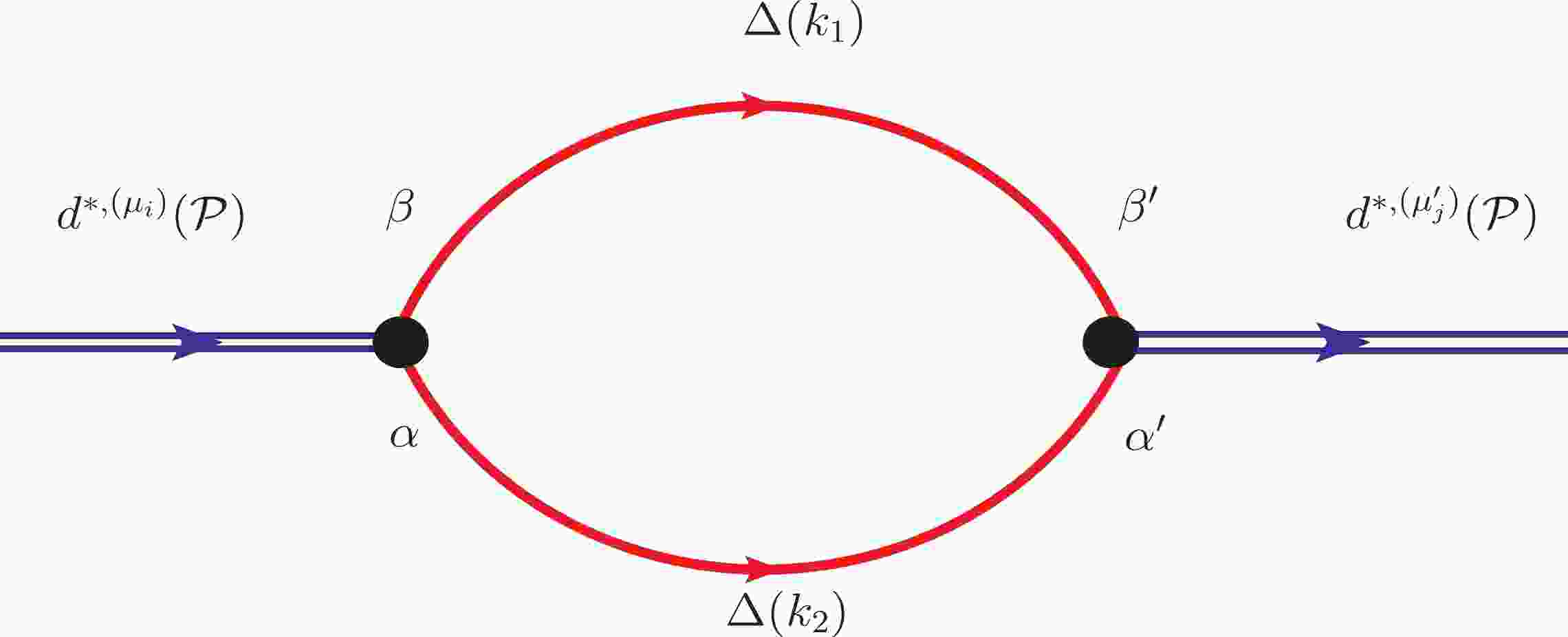
$ (c) $ stands for the channel of$ ({\Delta}{\Delta}) $ or$ (CC) $ , respectively, and$ P_c $ stands for the probability of the individual channel (c). The mass operator of$ {d^*} $ dressed by the$ \Delta\Delta $ loop is given in Fig. 1. It should be stressed that the effective coupling constant, determined by Eq. (4), contains the renormalization effect given that the chain approximation is considered (see, for example, Refs. [52, 54]). The explicit expression of the full mass operator of Fig. 1 and the effective coupling constant$ g_{{{d^*}\Delta\Delta}} $ have been demonstrated explicitly in Ref. [38].
Figure 1. (color online) Mass operator of
$ {d^*}(2380) \to {\Delta}{\Delta} $ .As we phenomenologically adopt the Gaussian-type correlation function of
$ \tilde\Phi(-p^2) = \exp(p^2/\Lambda^2) $ , there exists a model-dependent parameter Λ which relates to the size of the system in the non-relativistic approximation, at least in the physical sense. Consequently, we may roughly connect the size parameter of b in the non-relativistic wave function to the parameter Λ by$ b^2/2\sim 1/\Lambda^2 $ because the Gauss-like wave function$ \exp[-b^2\vec{p}^{2}/2] $ is often selected in the quark model calculation. Moreover, because$ b\sim 0.8\; {\rm fm} $ in the calculation of Refs. [13, 15], we roughly take the model parameter Λ here as$ \sim 0.34\; {\rm GeV} $ . -
We know that the forthcoming experiments at
$ {{\bar{{{\rm{P}}}}}} $ anda are related to the reactions of the antiproton beam colliding with the proton target. In this type of experiment, the baryon number of the initial states is zero. Meanwhile, according to the interpretations of$ {d^*} $ in our previous constituent quark model calculation [13, 15−17],$ {d^*} $ contains approximately 1/3$ |{\Delta}{\Delta}> $ and 2/3$ |CC> $ and, in particular, the$ |{\Delta}{\Delta}> $ component is primarily responsible for the decay of$ {d^*} $ . Therefore, to produce the dibaryon$ {d^*} $ at$ {{\bar{{{\rm{P}}}}}} $ anda in the final state of the$ {d^*}{\bar{{d^*}}} $ pair or$ {d^*}{\bar{p}}{\bar{n}} $ , the$ {\Delta}{\bar{{\Delta}}} $ intermediate state is essential. -
There are a few experiments for the
$ p{\bar{p}}\to \Delta(1232)\times {\bar{\Delta}}(1232) $ process in the literature [55−59] at$ \sqrt{s}=7.23 $ and$ 12\; {\rm GeV} $ . They were carried out from the large exposures of the$2\;{\rm m}$ hydrogen bubble-chamber (HBC) experiment to the U5 antiproton beam at CERN. The account of the final four-body system of$ p{\bar{p}}\pi^+\pi^- $ is believed to be primarily derived from the$ {\Delta}^{++}\overline{{\Delta}^{++}} $ channel. The collected data for the$ p{\bar{p}}\to \Delta(1232){\bar{\Delta}}(1232) $ reaction at$ 3.6 $ and$ 5.7\; {\rm GeV} $ confirm the conclusion drawn by Wolf in [60] that the t-channel pion or reggized pion exchange is a dominant mechanism responsible for this process. In other words, in terms of the t-channel one-pion-exchange (OPE) model, the mentioned reaction can be well-described. In particular, the total cross section of this process, in terms of the CM energy s, is empirically parameterized as$ \sigma (s)=As^{-n} $ with$ A=(67\pm 20)\; {\rm mb} $ and$ n= 1.5\pm 0.1 $ , respectively [58].As the reaction of
$ p{\bar{p}}\to \Delta{\bar{\Delta}} $ can be reasonable reproduced by using an effective Lagrangian, we simply write down the phenomenological effective Lagrangian in the following form [61]:$ \begin{eqnarray} {\cal L}^{(t_{z}^{\Delta}t_z^N)}_{\pi N\Delta}=g_{{\pi N\Delta}}F(p_t){\bar{{\Delta}}}_{\mu}^{(t_z^{{\Delta}})}\vec{\cal I}_{t_z^{{\Delta}}t_z^{N}}\cdot\partial^{\mu} \vec{\pi}^{(t_z^{\pi})}N^{(t_z^{N})}\, +\, {\rm h.c.}, \end{eqnarray} $

(5) where
$ g_{{\pi N\Delta}} $ is the effective coupling constant and$ F(p_t) $ stands for the phenomenological form factor, which is taken as$ \begin{eqnarray} F(p_t)=\Bigg(\frac{\Lambda_M^{*2}-m_{\pi}^2}{\Lambda_M^{*2}-p_t^2}\Bigg )\exp(\alpha p_t^2), \end{eqnarray} $

(6) with the parameters
$ \Lambda_M^{*}\sim 1\;{\rm GeV} $ . In Eq. (5),$ \vec{\cal I}_{t_z^{{\Delta}}t_{z}^{N}}= C_{1t_{\pi},1/2t_z^N}^{3/2t_z^{{\Delta}}}\hat{e}^*_{t_{\pi}} $ is the isospin transition operator. Detailed discussions of the matrix element, model parameter, and resultant cross section in the calculation of the$ p{\bar{p}}\to \Delta{\bar{\Delta}} $ process have been shown in our previous work [38]. The numerical result shows that the tree diagram reasonably reproduces the total cross section of$ p{\bar{p}}\to {\Delta}^{++}\overline{{\Delta}^{++}} $ , although we do not consider the contributions from other meson exchanges, for instance, the ρ meson exchange. In short, the effective Lagrangian$ {\cal L}^{(t_{z}^{\Delta}t_z^N)}_{{\pi N\Delta}} $ of Eq. (5) is qualitatively suitable for describing the cross section of the$ p{\bar{p}}\to \Delta{\bar{\Delta}} $ process and thus can also apply to the studies of the$ p{\bar{p}}\to \Delta{\bar{\Delta}}\to d^*{\bar{d^*}} $ and$ p{\bar{p}}\to \Delta{\bar{\Delta}} \to {d^*}{\bar{p}}{\bar{n}} $ reactions. -
In our previous work, the production rate of the two-body final state
$ {d^*}{\bar{{d^*}}} $ pair is estimated in the center-of-mass energy region of$ {{\bar{{{\rm{P}}}}}} $ anda. Here, the study in this aspect is extended to the calculation of the production rate of the three-body final state$ {d^*}{\bar{p}}{\bar{n}} $ or$ {\bar{{d^*}}}pn $ . The Feynman diagrams of$ p{\bar{p}}\to {d^*}{\bar{p}}{\bar{n}} $ via the$ {\Delta}{\bar{{\Delta}}} $ intermediate state are plotted in Fig. 2, where Fig. 2(a) shows that$ {\bar{p}} $ and$ {\bar{n}} $ are produced in the decay of the intermediate$ {\bar{{d^*}}} $ state, and compared with this subdiagram, Fig. 2(b) exhibits that$ {\bar{p}} $ and$ {\bar{n}} $ are produced in the reaction of two intermediate$ {\bar{\Delta}} $ states. Therefore, in detecting$ {\bar{d^{*}}} \to {\bar{p}}\,+\, {\bar{n}} $ in Fig. 2(a), (b) will be an important "background." It should be mentioned that both the single$ {d^*} $ and$ {d^*}{\bar{{d^*}}} $ pair in the subdiagrams of Fig. 2 are all generated from the$ p{\bar{p}}\to\Delta{\bar{\Delta}} $ annihilation reaction. This is because, in the loop diagrams in Fig. 2, when Δ interacts with Δ (or$ {\bar{\Delta}} $ interacts with$ {\bar{{\Delta}}} $ ), a corresponding hidden-color component$ CC $ (or$ {\bar{C}}{\bar{C}} $ ) would be formed in the symmetry re-arrangement. Further, in the higher order loop calculation, while$ p{\bar{p}} $ annihilate to generate a$ \Delta{\bar{\Delta}} $ pair, it can also create a corresponding$ C{\bar{C}} $ pair in the short range. According to the conclusion drawn in our previous quark model calculations, the structure of$ {d^*} $ can be written as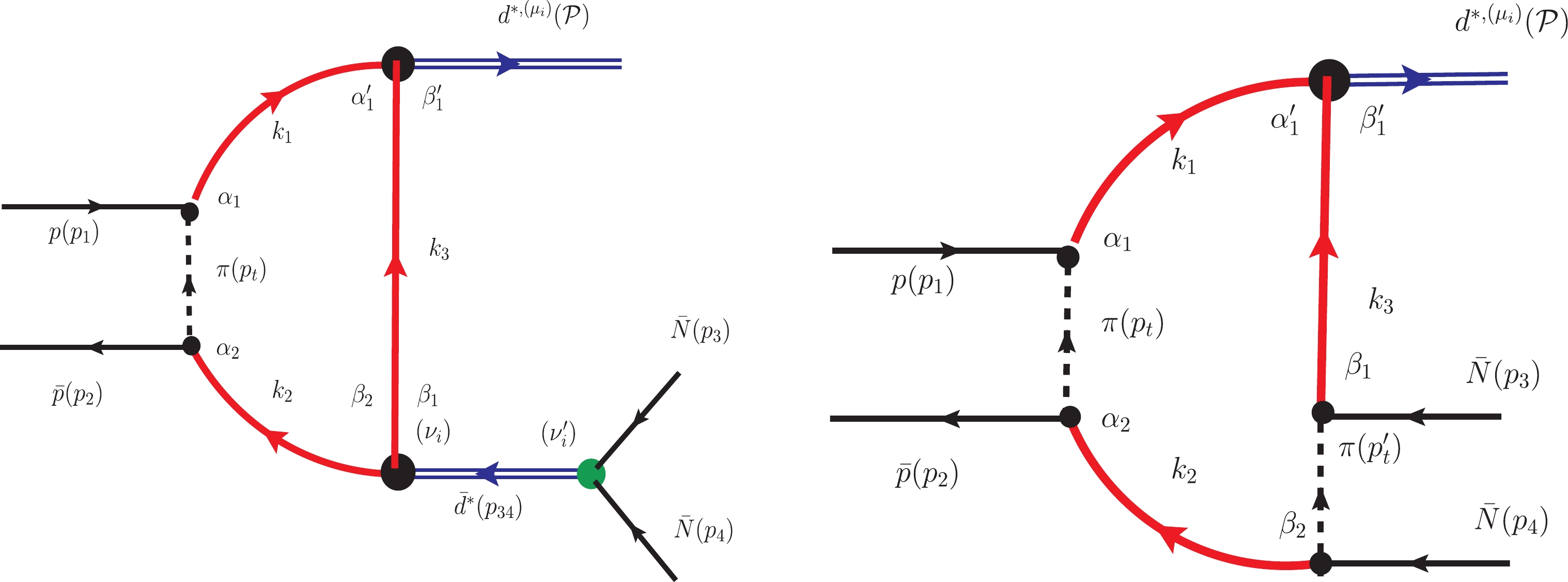
Figure 2. (color online) Feynman diagrams for the process of
$ p{\bar{p}}\to {d^*}(2380)+{\bar{p}}+{\bar{n}} $ via$ {\Delta}\overline{{\Delta}} $ intermediates. The two final states$ ({\bar{N}}(p_3) $ and$ {\bar{N}}(p_4)) $ stand for either$ ({\bar{p}}(p_3),{\bar{n}}(p_4)) $ or$ ({\bar{n}}(p_3),{\bar{p}}(p_4)) $ , respectively.$ \begin{eqnarray*} |{d^*}>\sim \sqrt{\frac{1}{3}}|{\Delta}{\Delta}>+\sqrt{\frac{2}{3}}|CC>, \end{eqnarray*} $

with the spin and isospin quantum numbers of the colored cluster C being 3/2 and 1/2. Because the observed
$ ({d^*})^+ $ is isoscalar, in the isospin space, the above$ |{\Delta}{\Delta}, I=0> $ can be re-written explicitly as$ \begin{eqnarray} |{\Delta}{\Delta}, I=0>=\frac12\big [|{\Delta}^{++}{\Delta}^->+|{\Delta}^+{\Delta}^0>+|{\Delta}^{0}{\Delta}^+>+|{\Delta}^-{\Delta}^{++}>\big ], \end{eqnarray} $

(7) namely, only the components of
$ |{\Delta}^{++}{\Delta}^{-}> $ and$ |{\Delta}^{+}{\Delta}^0> $ contribute to$ {d^*}(2380) $ . In addition, we stress that the reaction$ p{\bar{p}}\to {d^*}+{\bar{p}}+{\bar{n}} $ may occur above the energy threshold of$\sqrt{s}_0=M_{{d^*}}+2M_N\sim 4.256\; {\rm GeV}$ . This threshold is lower than the production threshold of the$ {d^*}{\bar{{d^*}}} $ pair ($ 2M_{{d^*}}\sim 4.47\; {\rm GeV} $ ), and also the upper limit of the center-of-mass energy of the$ {{\bar{{{\rm{P}}}}}} $ anda facility. -
Figure 2(a) shows the contribution of the
$ {d^*}{\bar{{d^*}}} $ production reaction to the specific process considered, where the outgoing$ {\bar{p}} $ and$ {\bar{n}} $ are produced in the decay of the$ {\bar{{d^*}}} $ resonance. The reason to consider this process is that the dibaryon$ {d^*} $ has a decay mode of$ {d^*}\to pn $ . Although this mode is not a so-called "golden" mode [7, 8], such as$ d\pi\pi $ or$ pn\pi\pi $ , its branching rate of approximately$ 10\% $ is still sizeable. From the experimental point of view, this type of events is detectable because$ {\bar{p}} $ and$ {\bar{n}} $ originate from the decay of the same$ {\bar{d^*}} $ . Meanwhile, the other class of events, where$ {\bar{p}} $ and$ {\bar{n}} $ originate from the reaction of two$ {\bar{\Delta}} $ , as shown in Fig. 2(b), despite a much larger cross section, is difficult to measure experimentally due to the large background. Therefore, in the$ p{\bar{p}}\to{d^*}{\bar{p}}{\bar{n}} $ calculation where only one dibaryon will be generated in the final state, one has to consider the important process of$ p{\bar{p}}\to {d^*}{\bar{{d^*}}}\to {d^*}{\bar{p}}{\bar{n}} $ , although$ {\bar{{d^*}}} $ is off-shell and the contribution from this mode might not be remarkable. To describe the subprocess of$ {d^*}\to pn $ , we simply adopt an effective Lagrangian$ {\cal L}_{{d^*} pn} $ as$ \begin{eqnarray} {\cal L}_{{d^*} pn}=g_{_{{d^*} pn}}q^{(pn)}_{\mu_1}q^{(pn)}_{\mu_2}{\bar{\psi}}_N \gamma_{\mu_3}\psi_N^C\times \big ({d^*}({{\cal P}})\big )^{(\mu_i)}\, +{\rm h. c.}, \end{eqnarray} $

(8) with
$ q^{(pn)} $ being the relative momentum between the proton and neutron, and$ \big ({d^*}({{\cal P}})\big)^{(\mu_i)} $ being the field of$ {d^*} $ with spin 3. As the experimentally measured branching ratio of$ {d^*}\to pn $ is approximately$ 10\% $ , the measured partial decay width is therefore approximately$ 7\; {\rm MeV} $ . Then, we can extract the value of the effective coupling constant as$ g_{{{d^*} pn}}\sim 1.01\; {\rm GeV}^{-2} $ .We can write the matrix element of Fig. 2(a) as
$ \begin{aligned}[b]\\[-8pt] {\cal M}_{2a}=&\int \frac{{\rm d}^4p_t}{(2\pi)^4{\rm i}}\Bigg [{\bar{v}}_N(p_2)\Big [p_{t}^{\alpha_2}{{\tilde S}}_{\alpha_2\beta_2}(k_2)\Gamma^{\beta_2\; \; \; \beta_1}_{\; \; (\nu_i)} {{\tilde S}}^C_{\beta_1\beta_1'}(k_3)\Gamma^{\beta_1'\; \; \; \alpha_1'}_{\; \; (\mu_i)} {{\tilde S}}_{\alpha_1'\alpha_1}(k_1)p_{t}^{\alpha_1}\Big ] u_N(p_1)\Bigg ] \\ &\times \big ({d^*}({{\cal P}})\big )^{*,(\mu_i)}\times\frac{g_{\pi N{\Delta}}^2g_{{{d^*} pn}}{\rm e}^{2{\alpha} p_{t;M}^2}}{p_t^2-m_{\pi}^2+{\rm i}\epsilon} \Bigg(\frac{\Lambda_M^{*2}-m_{\pi}^2}{\Lambda_M^{*2}-p_t^2}\Bigg )^2 \times\frac{{{\tilde \epsilon}}^{(\nu_i),(\nu'_j)}(p_{34})}{p_{34}^2-M_{{d^*}}^2+{\rm i}\Gamma_{{d^*}}M_{{d^*}}}\times (q_{34})_{\nu'_1}(q_{34})_{\nu'_2}\Big [{\bar{u}}^C_N(p_3)\gamma_{\nu'_3}v_N(p_4)\Big ], \end{aligned} $ 
(9) where
$ q_{34}=(p_3-p_4)/2 $ ,$ p_{34}=p_3+p_4 $ , and the relations of$ \hat{C}{\bar{u}}^T(\vec{p},s)=v(\vec{p},s) $ and$ \hat{C}{\bar{v}}^T(\vec{p},s)=u(\vec{p},s) $ are used. Moreover, in Eq. (9),$ \begin{aligned}[b] {{\tilde \epsilon}}_{(\mu\nu\sigma;{\alpha}\beta\gamma)}=&\sum_{pol.}\epsilon_{\mu\nu\sigma}\epsilon^*_{\alpha\beta\gamma}=\frac16\Big [{\tilde g}_{\mu\alpha}\Big ({\tilde g}_{\nu\beta}{\tilde g}_{\sigma\gamma} +{\tilde g}_{\nu\gamma}{\tilde g}_{\sigma\beta}\Big ) \\&+{\tilde g}_{\mu\beta}\Big ({\tilde g}_{\nu\alpha}{\tilde g}_{\sigma\gamma} +{\tilde g}_{\nu\gamma}{\tilde g}_{\sigma\alpha}\Big ) +{\tilde g}_{\mu\gamma}\Big ({\tilde g}_{\nu\alpha}{\tilde g}_{\sigma\beta} +{\tilde g}_{\nu\beta}{\tilde g}_{\sigma\alpha}\Big ) \Big ]\\ &-\frac{1}{15}\Big [{\tilde g}_{\mu\nu}\Big ({\tilde g}_{\sigma\alpha}{\tilde g}_{\beta\gamma} +{\tilde g}_{\sigma\beta}{\tilde g}_{\alpha\gamma} +{\tilde g}_{\sigma\gamma}{\tilde g}_{\alpha\beta}\Big ) \\&+{\tilde g}_{\mu\sigma}\Big ({\tilde g}_{\nu\alpha}{\tilde g}_{\beta\gamma} +{\tilde g}_{\nu\beta}{\tilde g}_{\alpha\gamma} +{\tilde g}_{\nu\gamma}{\tilde g}_{\alpha\beta}\Big )\\ & +{\tilde g}_{\nu\sigma}\Big ({\tilde g}_{\mu\alpha}{\tilde g}_{\beta\gamma} +{\tilde g}_{\mu\beta}{\tilde g}_{\alpha\gamma} +{\tilde g}_{\mu\gamma}{\tilde g}_{\alpha\beta}\Big ) \Big ],\\[-6pt] \end{aligned} $

(10) with
$ {\tilde g}^{\alpha\beta}=-g^{\alpha\beta}+\dfrac{p_{34}^{\alpha}p_{34}^{\beta}}{M_{{d^*}}^2} $ .$ \Gamma^{\beta_1',(\mu_i),\alpha_1'}= \Gamma_0^{\beta_1',(\mu_i),\alpha_1'} \exp\big [-q^2_E/\Lambda^2\big] $ contains a Lorentz structure$ \Gamma_0^{\,\beta_1',(\mu_i),\alpha_1'} $ of$ {d^*} (J^P=3^+) $ (see Eq. (2)) as well as a scalar correlation function$ \exp\big [-q^2_E/\Lambda^2\big] $ , which is a function of the relative momentum$ q_E $ between the two constituents of$ {d^*} $ .$ {{\tilde S}}_{{\alpha}\beta} $ stands for the propagator of the Rarita-Schwinger field. In addition, one takes the total width of$ \Gamma_{{d^*}}\sim 70\; {\rm MeV} $ in the Breit-Wigner form of the$ {d^*} $ propagator. -
Figure 2(b) exhibits another
$ p{\bar{p}} $ reaction process, which generates a three-body final state that includes a single dibaryon$ {d^*} $ , a$ {\bar{p}} $ , and a$ {\bar{n}} $ . This process is different from that in Fig. 2(a), since the outgoing$ {\bar{p}} $ and$ {\bar{n}} $ are produced by the final state interaction between$ {\bar{{\Delta}}} $ and$ {\bar{{\Delta}}} $ . Here, we also employ a t-channel pion exchange approach to describe this final state interaction. Then, the matrix element of Fig. 2(b) reads$ \begin{aligned}[b] {\cal M}_{2b}=&\int \frac{{\rm d}^4p_t}{(2\pi)^4{\rm i}}\Bigg [{\bar{v}}_N(p_2) \Big [p_{t}^{\alpha_2}{{\tilde S}}_{\alpha_2\beta_2}(k_2)p_{t}^{'\beta_2}\Big ]v_N(p_4)\Bigg ] \\&\times\Bigg[{\bar{u}}^C(p_3)\Big [p_{t}^{'\beta_1}{{\tilde S}}^C_{\beta_1\beta_1'}(k_3)\Gamma^{\beta_1'\; \; \; \alpha_1'}_{\; \; (\mu_i)} {{\tilde S}}_{\alpha_1'\alpha_1}(k_1)p_{t}^{\alpha_1}\Big ] \end{aligned} $

(11) $ \begin{aligned}[b] \quad&\times u_N(p_1)\Bigg ]\big ({d^*}({{\cal P}})\big )^{*,(\mu_i)} \times\frac{{\rm e}^{2{\alpha} (p_{t}^2+p^{'2}_{t})}}{p_{t}^2-m_{\pi}^2} \frac{g^4_{\pi N{\Delta}}}{p^{'2}_{t}-m_{\pi}^2} \\&\times \Bigg (\frac{\Lambda_M^{*2}-m_{\pi}^2}{\Lambda_M^{*2}-p_{t}^2} \cdot\frac{\Lambda_M^{*2}-m_{\pi}^2}{\Lambda_M^{*2}-p^{'2}_{t}}\Bigg )^2. \end{aligned} $

(11) -
Now, let us define following Mandelstam variables:
$ s_0=\big (p_1+p_2\big)^2 $ for the initial states,$ s_1=\big ({{\cal P}}+p_3\big)^2 $ and$s_3= \big ({{\cal P}}+p_4\big)^2$ for the outgoing$ {d^*} $ and one of the two anti-nucleons, and$ s_2=\big (p_3+p_4\big)^2 $ for the two outgoing anti-nucleons, where the identity of$s_1+s_2+s_3= s_0+M^2_{{d^*}}+M_3^2+ M^2_4 $ holds. Then, the invariant mass spectrum of$ {\bar{p}} $ and$ {\bar{n}} $ for Fig. 2(a) can be expressed as$ \begin{eqnarray} \frac{{\rm d}\sigma_{(2a)}}{{\rm d}\sqrt{s_2}}= \int_{s_1^-}^{s_1^+} {\rm d}s_1 \frac{2\sqrt{s_2}\;\big|\overline{{\cal M}\;\big|}_{\rm Fig. 2(a)}^2}{16(2\pi)^3s_0 \sqrt{(p_1\cdot p_2)^2-m_1^2m_2^2}}, \end{eqnarray} $

(12) where the integral limits caused by the energy conservation are
$ \begin{aligned}[b] s_1^{\pm}=&M_{d^*}^2+m_3^2-\frac{1}{2s_2} \Big [\big (s_2-s_0+M_{d^*}^2\big )\big (s_2+m_3^2-M_{d^*}^2\big )\\&\mp \lambda^{1/2}\big (s_2,s_0,M_{d^*}^2\big ) \lambda^{1/2}\big (s_2,m_3^2,m_4^2\big )\Big ], \end{aligned} $

(13) with
$ \begin{eqnarray} \lambda(x,y,z)=x^2+y^2+z^2-2xy-2yz-2zx. \end{eqnarray} $

(14) It should be mentioned that the variable
$ s_2=\big (p_3+p_4\big)^2 $ is the squared invariance mass of the outgoing anti-proton and anti-neutron in Fig. 2(a); therefore, the invariant mass spectrum$ {\rm d}\sigma_{2(a)}/{\rm d}\sqrt{s_2} $ describes the distribution of the final$ {\bar{p}}{\bar{n}} $ pair originated from the$ {\bar{{d^*}}} $ resonance.Moreover, the total cross section of
$ p{\bar{p}}\to {d^*}+{\bar{p}}+{\bar{n}} $ via the$ {\Delta}{\bar{{\Delta}}} $ intermediate state, contributed by both Fig. 2(a) and (b), reads$ \begin{eqnarray} \sigma= \int_{s_2^-}^{s_2^+} {\rm d}s_2 \Bigg [\frac{{\rm d}\sigma_{(2a)}+{\rm d}\sigma_{(2b)}}{{\rm d}s_2}\Bigg ], \end{eqnarray} $

(15) with the integral limits being
$ \begin{eqnarray} s_2^-=(m_3+m_4)^{2},\; \; \; \; \; s_2^+=(\sqrt{s_0}-M_{d^*})^2. \end{eqnarray} $

(16) In Eq. (15),
$ {\rm d} \sigma_{(i)}/{\rm d} s_2 = \dfrac{1}{2\sqrt{s_2}} \big ({\rm d} \sigma_{(i)}/{\rm d} \sqrt{s_2}\big) $ with$ i=2(a) $ or$ 2(b) $ , and$ {\rm d} \sigma_{2(b)}/{\rm d} \sqrt{s_2} $ has the same form as that in Eq. (12), except that Fig. 2(a) changes to Fig. 2(b). -
In this work, we use the PELA to describe the spin-3 resonance
$ {d^*} $ and use the relativistic covariant field approach to calculate the$ p{\bar{p}}\to {d^*}{\bar{p}}{\bar{n}} $ process via the$ {\Delta}\overline{{\Delta}} $ intermediate state. In the latter approach, we have a model-free parameter Λ. To roughly estimate the value of this parameter, some of the qualitative conclusions given in the study of$ {d^*}(2380) $ with a constituent quark model [16] are simply taken into account. Those conclusions are as follows: 1) it is a compact hexaquark-dominant system; 2) it contains approximately 2/3 hidden color component and only approximately 1/3$ {\Delta}{\Delta} $ component; and 3) its decay properties are mainly determined by its$ {\Delta}{\Delta} $ component. Moreover, when$ b\sim 0.8\; {\rm fm} $ , the value of the model parameter Λ is approximately equal to$ 0.34\; {\rm GeV} $ because$ \Lambda^2 \sim {2}/{b^2} $ . In terms of Eq. (4), one can extract the effective coupling constant of$ {d^*} $ to$ \Delta\Delta $ by taking$ P_{\Delta\Delta} \sim 1/3 $ (see Ref. [38] for details). To demonstrate the Λ-dependence of the final results, we also change the value of Λ around$ 0.34\; {\rm GeV} $ , say$ 0.30\; {\rm GeV} $ or$ 0.40\; {\rm GeV} $ , in the calculation.Here, we mention again that the sub-processes of
$ p{\bar{p}}\to{\Delta}{\bar{{\Delta}}} $ and$ {\bar{{\Delta}}}{\bar{{\Delta}}}\to{\bar{p}}{\bar{n}} $ are simply treated by using a t-channel one-pion exchange approach, and, in terms of an effective Lagrangian approach, the subprocess of$ {d^*}\to pn $ decay in Fig. 2(a) is phenomenologically considered by comparing with the measured partial decay width. The values of model parameters used in the calculation are presented in Table 1.t-channel π exchange ${d^*} \to pn$ 

$g_{ { {\Delta}\pi N} }/{\rm GeV}^{-1}$ 

$\Lambda_M^*/{\rm {\rm GeV}}$ 

$\alpha/{\rm GeV}^{-2}$ 

$g_{{{d^*} pn}}/{\rm GeV}^{-2}$ 

$10.75$ 

$1.0$ 

$0.4$ 

$1.01$ 

Table 1. Parameters used in the calculation.
-
In the region of the CM energy
$ \sqrt{s_0}\in[4.4-5.5]\; {\rm GeV} $ , the total cross sections of the$ p{\bar{p}}\to {d^*}+{\bar{p}}{\bar{n}} $ process through the intermediate state of$ \Delta\overline{\Delta} $ , shown in Fig. 2(a) and 2(b), are calculated, and the corresponding curves are plotted in Fig. 3(a) and 3(b), respectively. To show the dependence of the model parameter Λ, the cross sections with$ \Lambda=0.30,\; 0.34 $ , and$ 0.40\;{\rm GeV}$ are also plotted in Fig. 3(a) and 3(b).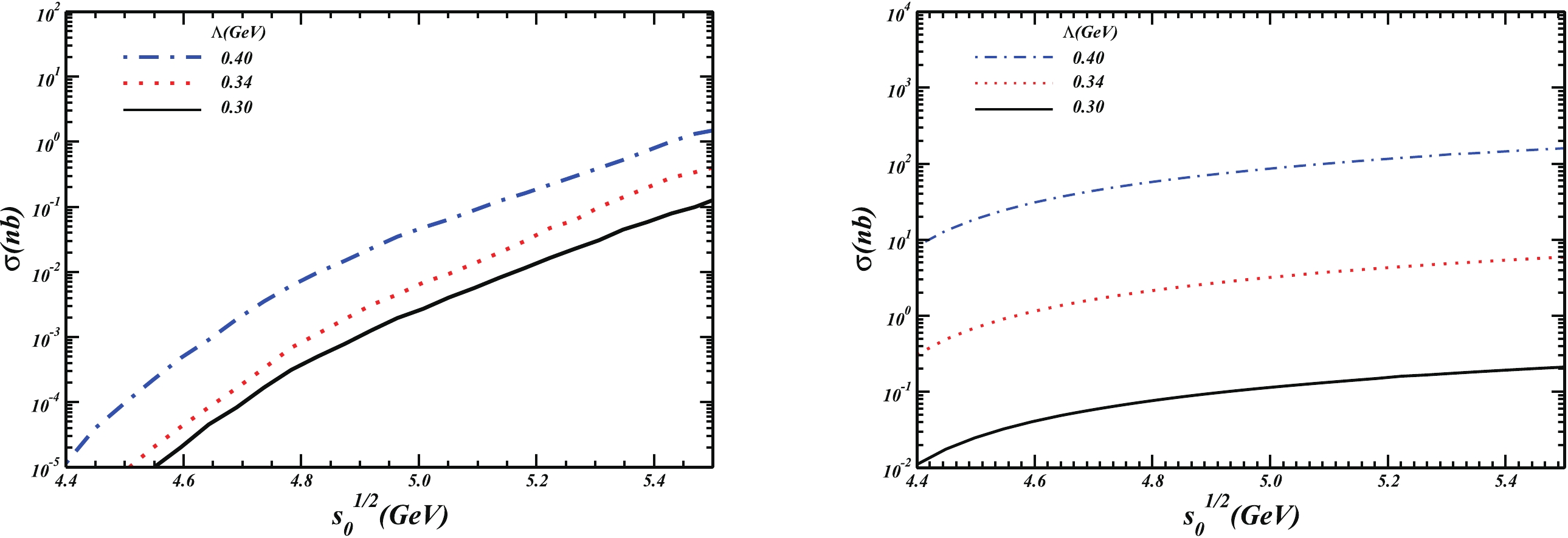
Figure 3. (color online) Numerical results for the total cross section of
$ p{\bar{p}}\to {d^*}+{\bar{p}}{\bar{n}} $ via$ {\Delta}{\bar{{\Delta}}} $ intermediate with CM energy ($ \sqrt{s_0} $ ) being$ (4.4\; -\; 5.5) $ GeV. The left and right panels show the results contributed by Fig. 2(a) and (b), respectively. In both figures, the black-solid, red-dotted, and blue-dotted-dashed curves display the results with Λ being$ 0.30 $ ,$ 0.34 $ , and$ 0.40 $ GeV, respectively.It is known that the cross sections of the diagrams shown in Fig. 2 depend not only on the size of the matrix elements
$ {\cal M}_{2a} $ and$ {\cal M}_{2b} $ , but also on the size of the phase space. The phase space increases with the increase in$ \sqrt{s}_0 $ . The matrix elements$ {\cal M}_{2a} $ and$ {\cal M}_{2b} $ depend on the model parameter Λ, the initial state energy$ \sqrt{s}_0 $ , and the loop integral as well. Therefore, the estimated values of the total cross sections for the considered processes are deeply influenced by the interpretation of the$ {d^*} $ resonance, i.e., its size and structure, namely, the probability of its$ \Delta\Delta $ component. In this work the cross section is evaluated based on the three qualitative interpretations of$ {d^*} $ drawn in the non-relativistic quark model calculation [15, 16], where$ P_{\Delta\Delta}\sim 1/3 $ . Actually, the effective coupling constant$ g_{{{d^*}{\Delta}{\Delta}}} $ is proportional to$ \sqrt{P_{\Delta\Delta}} $ , and the matrix element$ {\cal M}_{2} $ is proportional to$ P^2_{\Delta\Delta} $ in Fig. 2(a) and to$ P_{\Delta\Delta} $ in Fig. 2(b). In this way, the resultant cross sections will change as$ P_{\Delta\Delta} $ changes. In addition, the effective coupling constant$ g_{_{{d^*}{\Delta}{\Delta}}} $ and matrix elements$ {\cal M}_{2(a)} $ and$ {\cal M}_{2(b)} $ are closely related to the structure of the mass operator in the structural integrals in Fig. 1 and to the loop integral in Fig. 2. Therefore, the explanation for the behavior of the cross section curve here is the same as the explanation for the cross section behavior of the$ p{\bar{p}} \to \Delta{\bar{\Delta}} \to {d^*}{\bar{{d^*}}} $ process in our previous paper [38]. We will not repeat it here. Interested readers can refer to [38]. Furthermore, it should be noted that the cross section is sensitive to the value of Λ and even more sensitive in the calculation of Fig. 3(a) than in the evaluation of Fig. 3(b). This is because there are two correlation functions in Fig. 2(a) but only one correlation function in Fig. 2(b).Now, let us look at the magnitude of the cross section. It is approximately
$ 2.0\times 10^{-1}\sim 6.0\;{\rm nb} $ in Fig. 3(b) when$\Lambda\sim 0.34$ GeV, but only approximately$ 1.0\times 10^{-6}\sim 4.0\times 10^{-1}\; {\rm nb} $ in Fig. 3(a). Comparing the results in Figs. 3(a) and (b), we find that the cross sections in Fig. 3(b) are approximately 2−3 orders larger than those in Fig. 3(a). This is because the final anti-proton and anti-neutron are produced by the$ {\bar{{\Delta}}}{\bar{{\Delta}}} $ t-channel reaction in Fig. 2(b), but by the strong decay of the$ {\bar{{d^*}}} $ resonance ($ {\bar{{d^*}}}\to {\bar{p}}{\bar{n}} $ ), which only has a branching ratio of approximately$ 10\% $ , in Fig. 2(a). The effective coupling$ g^2_{\Delta \pi N} $ in the t-channel reaction is approximately 2 orders greater than the effective coupling$ g_{{d^*} p n} $ in the$ {\bar{{d^*}}} \to {\bar{p}}{\bar{n}} $ decay. Therefore, regardless of how we add the cross sections given by Fig. 2(a) and Fig. 2(b), constructively or destructively, the total cross section of Fig. 2 is almost equal to the cross section provided by Fig. 2(b). Namely, compared with Fig. 2(a), (b) plays a super-dominant role.Moreover, in Fig. 4, we plot the invariant mass spectrum of the final outgoing anti-proton and anti-neutron, which are generated by the strong decay of the intermediate
$ {\bar{{d^*}}} $ state shown in Fig. 2(a). In this figure, one clearly sees a resonant structure around$ 2.38 $ GeV. It indicates that the source of the anti-proton and anti-neutron is$ {\bar{{d^*}}} $ .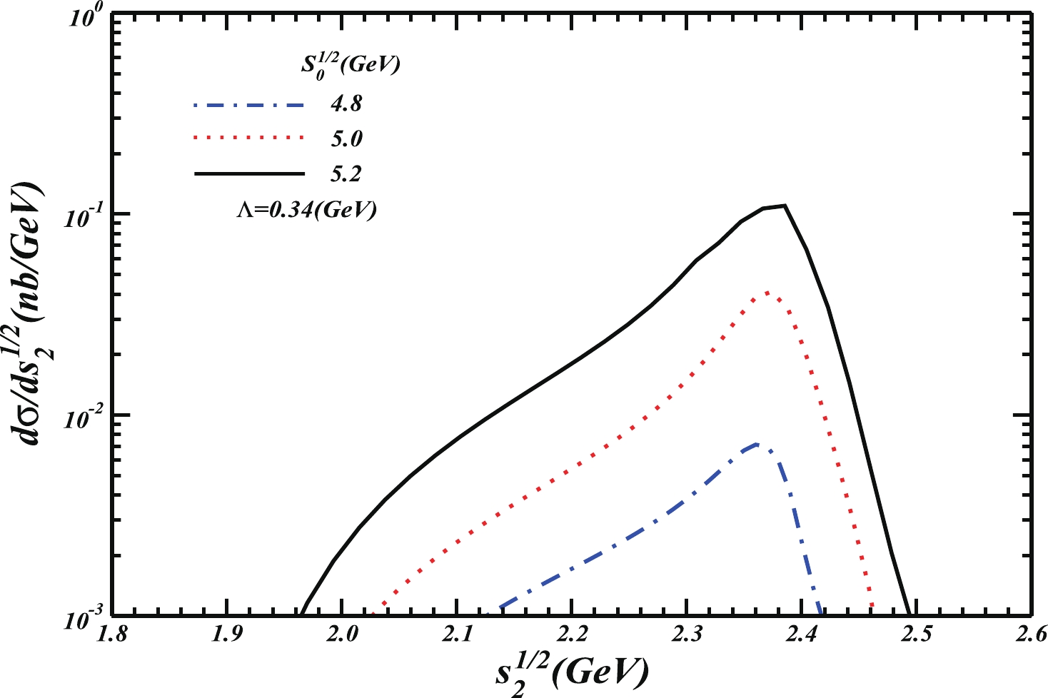
Figure 4. (color online) Numerical results for
$ {\rm d}\sigma/{\rm d}s^{1/2}_2 $ in the case of$ \Lambda=0.34\; {\rm GeV} $ . In the figure, the blue-dotted-dashed, red-dotted, and black-solid curves display the results with$ \sqrt{s_0} $ being$ 4.8 $ ,$ 5.0 $ , and$ 5.2 $ GeV, respectively.Here, we would emphasize again that although the cross section of Fig. 2(b) is relatively larger, it is difficult to measure owing to the huge background of
$ {\bar{p}} $ and$ {\bar{n}} $ in the$ p{\bar{p}} $ annihilation process. Meanwhile, although the cross section of Fig. 2(a) is much smaller than that of Fig. 2(b), it is measurable because$ {\bar{p}} $ and$ {\bar{n}} $ come from the same source. If we can obtain this invariant mass spectrum in the experiment, it can be used as one of the evidences for the existence of$ {\bar{{d^*}}} $ .At
$ \sqrt{s_0}\geq 4.5\; {\rm GeV} $ , based on the fact that the total cross section of$ p{\bar{p}}\to\Delta{\bar{\Delta}}\to {d^*}{\bar{p}}{\bar{n}} $ with$ \Lambda\sim 0.34\; {\rm GeV} $ is in the order of$ {\rm nb} $ , one can further estimate the number of events of such a process at$ {{\bar{{{\rm{P}}}}}} $ anda facility. Considering that the designed luminosity and integrated luminosity of this facility are approximately$\sim 2\times 10^{32}\;{\rm cm}^{-2}/{\rm s}$ and$\sim 1.7\times 10^{4} {\rm nb}^{-1}/{\rm d}$ , respectively, we expect that at$ \sqrt{s_0}=(4.8,\; 5.0, 5.2,\; 5.4)\; {\rm GeV} $ , if the overall efficiency is$ 100\% $ , approximately$ (3.63,\; 5.59,\; 7.23,\; 9.34)\times 10^{4} $ events of$ {d^*}{\bar{p}}{\bar{n}} $ could approximately be generated per-day, of which only approximately$ (20,\; 100,\; 600,\; 3200) $ events are derived from the process in Fig. 2(a). As mentioned above, although the number of the events derived from the$ {\bar{{d^*}}} \to {\bar{p}}{\bar{n}} $ mode are only approximately$ 3\%\sim 4\% $ of the total number of events or even smaller, they can be observed in the experiment. However, a large number of other events cannot be identified.Finally, we stress that in our previous discussion [62, 63], we have mentioned that in order to avoid the interference caused by the background of a large number of produced pions and nucleons, one can measure antiparticle
$ {\bar{{d^*}}} $ instead of$ {d^*} $ . Here, in the$ p{\bar{p}} \to {d^*} {\bar{{d^*}}} $ reaction,$ {d^*} $ can also decay through its "golden" decay channels of$ d\pi\pi $ and$ pn\pi\pi $ or through$ pn $ . Same as the reason mentioned above, the interference from the background makes it difficult to measure$ {d^*} $ . Therefore, we propose that based on the potentially huge data set in$ {{\bar{{{\rm{P}}}}}} $ anda, measuring two final$ {\bar{p}}{\bar{n}} $ generated from one$ {\bar{{d^*}}} $ is another possible method to identify$ {\bar{{d^*}}} $ with the background interference being bypassed. -
As an extension of our previous study on
$ p{\bar{p}}\to{d^*}{\bar{{d^*}}} $ via the$ {\Delta}{\bar{{\Delta}}} $ intermediate state, in this work, we further estimate the cross section of the$ p{\bar{p}}\to {d^*}{\bar{p}}{\bar{n}} $ (or$ p{\bar{p}}\to {\bar{{d^*}}}pn $ ) process, which might possibly occur and consequently be measured at the forthcoming experiments at the$ {\bar{P}} $ anda facility in the CM energy region of$ \sqrt{s}\in [4.4, 5.5]\; {\rm GeV} $ . The present process with the three-body final state is different from the previous one with the two-body final state of$ {d^*}{\bar{{d^*}}} $ because the outgoing anti-proton and anti-neutron (or proton and neutron in the process of$ p{\bar{p}}\to{\bar{{d^*}}}+pn $ ) can be produced not only by the decay of$ {\bar{{d^*}}} $ (or$ {d^*} $ ) but also by the re-scattering of the intermediate$ {\bar{{\Delta}}}-{\bar{{\Delta}}} $ (or$ {\Delta}-{\Delta} $ ) states.We employ the relativistic covariant PELA to roughly estimate the cross section and possible number of events. In describing the structure of the produced dibaryon
$ {d^*} $ or anti-dibaryon$ {\bar{{d^*}}} $ , we directly adopt the qualitative conclusions drawn from the sophisticated dynamic calculation of the structure of$ {d^*} $ in a non-relativistic constituent quark model and fix the model-parameter Λ. Our estimated cross section of this reaction is in the order of$ {\rm nb} $ , which is much smaller than that of the$ p{\bar{p}}\to\Delta{\bar{\Delta}} $ reaction of order$ {\rm mb} $ but much larger than that of the$ p{\bar{p}}\to{d^*}{\bar{{d^*}}}\to{d^*}{\bar{p}}{\bar{n}} $ process shown in Fig. 2(a). However, according to our estimation in this work, in the huge amount of data collected on the hadron pair production at$ {\bar{P}} $ anda facility, there is still a certain and even sizeable amount of$ {d^*}{\bar{p}}{\bar{n}} $ events if$ {d^*} $ exists, in particular, the events generated by the intermediate$ {\bar{{d^*}}} $ state. Certainly, one also expects to have a larger signal of the existence of$ {\bar{{d^*}}} $ from its "golden" decay channel$ {\bar{{d^*}}}\to {\bar{d}}+\pi\pi $ . However, the phase space of the four-body final state may suppress the cross section of the$ p{\bar{p}}\to {d^*}{\bar{d}}\pi\pi $ process. In any case, the study of this process is in progress. -
We would like to thank Prof. Zongye Zhang for valuable discussions.
An estimate of dibaryon production in the process of ${\boldsymbol p{{\bar{\boldsymbol p}}}\to\boldsymbol d^*({\bf 2380})+{\bar{\boldsymbol p}}{\bar{\boldsymbol n}} }$ at ${ {\bar{{\bf{P}}}}} $ anda facility
- Received Date: 2022-06-12
- Available Online: 2022-11-15
Abstract: Although


 DownLoad: