


 Abstract
 HTML
HTML Reference
 Related
 PDF
PDF


-
The historic observation of the Higgs boson in 2012 at the Large Hadron Collider (LHC) [1, 2] declared the discovery of the last missing piece of the most fundamental building blocks in the Standard Model (SM). The SM has been remarkably successful in describing experimental phenomena. However, a precision Higgs physics program would be critically important given that the SM does not predict the parameters in the Higgs potential, nor does it involve particle candidates for dark matter. The precision determination of the Higgs couplings to the SM particles, gauge bosons and leptons/quarks, are the agents probing the Higgs mechanism for generating masses [3]. In particular, potential observable deviations of the Higgs couplings from the SM expectations would indicate new physics [4]. Therefore, the Higgs discovery marks the beginning of a new era of both theoretical and experimental exploration. Various
$ e^+e^- $ colliders were proposed as Higgs factories by the high energy physics community, such as ILC [5], CLIC [6], FCC-ee [7], and CEPC [8, 9].The most important advantages of a Higgs factory are that the center of mass (CM) energy is precisely defined and that they could perform absolute measurements of the Higgs boson. Neglecting Z fusion production, in an
$ e^+e^-\to ZH $ event, where the Z decays into a pair of visible fermions or their stable decay final states ($Z\rightarrow e^+e^-,\; \mu^+\mu^-,\; \tau^+\tau^-,\; \rm{or}\; q\bar{q}$ ), the Higgs boson can be identified from the kinematics of those fermion pairs or their stable daughters independent of the Higgs decays. For example, the$ Z\to e^+e^- $ and$ \mu^+\mu^- $ modes are studied systematically in Refs. [10, 11]. The production cross-section and most of the decay branching fractions of the Higgs could be measured model-independently by the counting method. For example, CEPC could measure the cross-section of$ e^+e^-\rightarrow ZH $ ,$ \sigma(ZH) $ , at 240 GeV, to a precision of 0.5% and the branching fractions of the Higgs boson to a few percent, respectively, by combining the four decay modes of the Z boson [11, 9].The physics goal of a Higgs factory must be accomplished by optimizing the detector design and making use of the latest developments in data science. Recently, various Machine Learning (ML) techniques have already shown very promising performance in data analysis for high energy physics [12], in particular for jet studies. For instance, jets are treated as images [13–18], as sequences [19–22], as trees [23, 24], as graphs [25], or sets [26, 27] of particles, and ML techniques, most notably deep neural networks (DNNs), are used to build new jet tagging algorithms automatically from (labeled) simulated samples and even data [28–31]. While the above ML techniques are used at jet-level for case studies, they naturally can be applied for the event level in
$ e^+e^- $ collisions, which have much simpler topologies and are pile-up free.In this article, two ML approaches are used to study the classification problem of Higgs events. The classification results can serve as the basis of an "end-to-end" (E2E) analysis, which enables the simultaneous analysis of almost all the Higgs decays modes with the state-of-the-art ML techniques, starting with particle-level information and ending with physics observables. The approach also is a "one-stop" analysis to support extracting all Higgs couplings and taking into account the correlations and commonalities of the same detector for the experiment. Throughout this paper, the term "one-stop" analysis refers to an analysis method used to extract multiple observables of the same type at once. It differs from a conventional analysis in several ways. First, because many physics observables are measured using modern ML techniques at the same time, "one-stop" analysis is more efficient. Second, ML techniques usually deploy more information. Instead of only some limited number of selection criteria being used in conventional analysis, four-momenta and impact parameters (only charged tracks) of all particles in an event will be used by the ML techniques. Third, "one-stop" analysis could take into account the correlations and commonalities of the same detector for the experiment. Because all the measurements and their correlations are obtained in a consistent way, creating a combination based on these measurements will be easy.
The rest of this paper is organized as follows. The ML methods used in this study are introduced in Sec. II, followed by the implementation of the ML methods with a Monte Carlo (MC) simulation in Sec. III. Finally, a summary is presented.
-
Recently, various ML techniques were proposed for jet tagging studies. Among them, PFN [26] and ParticleNet [27] achieved superior performance.
In the original publication of PFN [26], the authors applied the Deep Sets concept [32] to the jet-tagging problem. They proposed two elegant model architectures, named EnergyFlow Network (EFN) and ParticleFlow Network (PFN), with provable physics properties, such as infrared and colinear safety. In these two architectures, the features of each particle are encoded into a latent space of Φ [32] and the category, F, is extracted from the summed representation in that latent space. Both Φ and F are approximated by neural networks. The key mathematical fact is that a generic function of a set of particles can be decomposed into an arbitrarily good approximation according to the Deep Set Theorem [32]. The performance of these models in classification problems is comparable with other more complicated models. The authors also tried to interpret and visualize what the model has learned [26].
Motivated by the success of CNNs, the ParticleNet [27] approach based on the Dynamic Graph Convolutional Neural Network (DGCNN) is proposed for learning on particle cloud data. The edge convolution ("EdgeConv") operation, a convolution-like operation for point clouds, is used instead of the regular convolution operation. One important feature of the EdgeConv operation is that it can be easily stacked, just like regular convolutions. Therefore, another EdgeConv operation can be applied subsequently, which makes it possible to learn features of point clouds hierarchically. Another important feature is that the proximity of points can be dynamically learned with EdgeConv operations. The study shows that the graph describing the point clouds is dynamically updated to reflect the changes in the edges, i.e., the neighbors of each point. Reference [27] shows that this leads to better performance than keeping the graph static.
As suggested by the authors [26] and according to the performances of EFN and PFN, we choose PFN and ParticleNet to classify the Higgs decays. This ML attempt contains some distinct features in contrast to conventional data analysis. First, the ML approach is used to classify many physics processes at the same time. If some tiny decays are neglected, there are about 9 branching fractions of the Higgs decays to be measured. The number of classes is greater than 9 when the SM backgrounds are included. In addition, the classification results could be the basis of an E2E analysis, which means that all the particle-level information, such as four-momenta, PID, and impact parameters of charged particles, is used as input directly, and the network calculates the scores of each event. In this case, the analysis no longer needs some dedicated and complicated reconstruction tools, such as lepton/photon isolation, jet-clustering, τ finder, etc.
-
In this section, four 9-category classifications of the all accessible Higgs decay final states are realized according to different Z decay modes with the PFN method, and their confusion matrices are determined. As a preliminary attempt, a more ambitious 39-category classification is tried with the ParticleNet, and promising and consistent results are achieved.
-
For the two ML models used to classify the Higgs decays, kinematic information of energy, polar and azimuthal angles are always given for each reconstructed particle. We should note that energies and polar angles are used instead of the transverse momenta and rapidities, respectively, in the original studies [26, 27] since the models are utilized for
$ e^+e^- $ collider experiments in this study. The inputs also include the PID and impact parameters of charged particles.The PFN architecture [26] is designed to parameterize the functions Φ and F in a sufficiently general way, using several dense neural network layers as universal approximators. For Φ, three dense layers are employed, with 100, 100, and l nodes respectively, where l is the latent dimension that takes 256 after comparing the performances of 128 and 256. For F, we use the same configuration as the original paper, which has three dense layers, each with 100 nodes. Each dense layer uses the
$ {\rm{ReLU}} $ activation function and He-uniform parameter initialization [33]. A nine-unit layer (depending on the number of classes) with a$ {\rm{SoftMax}} $ activation function is the output layer.The ParticleNet [27] architecture consists of three EdgeConv blocks, one aggregation layer, and two fully-connected layers. The first EdgeConv block uses the spatial coordinates of the particles in the
$ \theta-\phi $ space to compute the distances, while the subsequent blocks use the learned feature vectors as coordinates. The number of nearest neighbors k is 16 for all three blocks, and the number of channels C for each EdgeConv block is (64, 64, 64), (128, 128, 128), and (256, 256, 256), respectively. After the EdgeConv blocks, a channel-wise global average pooling operation is applied to aggregate the learned features over all particles in the cloud. This is followed by a fully-connected layer with 256 units and the ReLU activation. A dropout layer with a drop probability of 0.1 is included to prevent overfitting. A fully connected layer with 39 units, followed by a SoftMax function, is used to generate the output for the 39-category classification task. -
In this study, there are 4 production modes for the Higgs boson at 240 GeV to be analyzed, i.e.,
$e^+e^- \to e^+e^-H$ ,$ \mu^+\mu^-H $ ,$ \tau^+\tau^-H $ , and$ q\bar{q}H $ . In each production mode, the same 9 decay modes are measured, which are$ H \to c\bar{c} $ ,$ b\bar{b} $ ,$ \mu^+\mu^- $ ,$ \tau^+\tau^- $ ,$ gg $ ,$ \gamma\gamma $ ,$ ZZ^* $ ,$ WW^* $ , and$ \gamma Z $ , respectively. So there are 36 processes in total. For each process, 400,000 events are generated with WHIZARD 1.9.5 [34] and fed to Pythia6 [35] for hadronization, where decays of most intermediate particles, such as W, Z, and τ, etc., are also simulated by Pythia6 according to its default configuration, and the branching fractions of the Higgs are customized based on Table 1. All the cross sections and decay branching fractions used in this study are summarized in Table 1. The organization and description of 4-fermion backgrounds are complicated and need some sophisticated scheme. Here$ ZZ $ represents that the 4 fermions are produced via two (virtual) neutral vector bosons. More details can be found in Ref. [36]. It should also be noted that the sequential decays of W and Z are not dealt with specifically, to avoid complexity, though it can enhance the classification performance if more decay knowledge is used.Mode Cross section or branching fraction $ \sigma(e^+e^-\to e^+e^-H) $ 

7.04 fb $ \sigma(e^+e^-\to \mu^+\mu^-H) $ 

6.77 fb $ \sigma(e^+e^-\to \tau^+\tau^-H) $ 

6.75 fb $ \sigma(e^+e^-\to q^+q^-H) $ 

136.81 fb $ \sigma(e^+e^-\to ZZ_{l}) $ 

67.81 fb $ \sigma(e^+e^-\to ZZ_{sl}) $ 

516.67 fb $ \sigma(e^+e^-\to ZZ_{h}) $ 

556.49 fb $ B(H\to c\bar{c}) $ 

2.91% $ B(H\to b\bar{b}) $ 

57.7% $ B(H\to \mu^+\mu^-) $ 

$ 2.19\times 10^{-4} $ 

$ B(H\to \tau^+\tau^-) $ 

6.32% $ B(H\to gg) $ 

8.57% $ B(H\to \gamma\gamma) $ 

$ 2.28\times 10^{-3} $ 

$ B(H\to WW^*) $ 

21.5% $ B(H\to ZZ^*) $ 

2.64% $ B(H\to Z\gamma) $ 

$ 1.53\times 10^{-3} $ 

Table 1. Standard model predictions of the decay branching fractions and cross sections at 240 GeV of a 125 GeV Higgs boson, with their irreducible backgrounds at the CEPC.
All the generated samples are simulated in a simplified way to model detector responses. In detail, all particles are simulated according to the performance of the baseline detector in the CEPC CDR [9]. The momentum resolution of charged tracks is
$\frac{\sigma(p_t)}{p_t} = 2\times 10^{-5}\oplus \frac{0.001} {p\sin^{3/2}\theta}~ [\mathrm{GeV}^{-1}] .$

The energy resolution of photons is
$\frac{\sigma(E)}{E} = 0.01 \oplus \frac{0.20}{\sqrt{E/\mathrm{(GeV)}}},$

and that of neural hadrons is
$\frac{\sigma(E)}{E} = 0.03 \oplus \frac{0.50}{\sqrt{E/\mathrm{(GeV)}}},$

and all the reconstruction efficiencies are assumed to be 100% in the simulation. In the case of impact parameters and particle identification, they are taken directly from the truth of generation. While the simplified simulation is a bit too ideal, it is sufficient for a feasibility study. The performance is expected to get worse in the full simulation since the impact parameters are crucial for the separations among Higgs hadronic decays, especially for
$ b\bar{b}/c\bar{c}/gg $ . -
The ParticleFlow Network and ParticleNet are implemented and running with 8 Intel
$ ^\circledR $ Xeon$ ^\circledR $ Gold 6240 CPU cores and 8 NVIDIA$ ^\circledR $ Tesla$ ^\circledR $ V100-SXM2-32GB GPU cards at the IHEP GPU farm. During model training, the common properties of the neural networks include categorical cross-entropy loss function, the Adam optimization algorithm [37], a batch size of 1000, and a learning rate of 0.001. 400,000 events are used for each production mode, and the total number of events for 9 decays is 3,600,000. The full data set is split into training, validation, and test samples according to the ratio 8:1:1. The monitoring of loss and accuracy on training and validation samples shows that the models converge well and there is no obvious over-training after the models are trained for 100 epochs; see Fig. 1 as an example.
Figure 1. (color online) Accuracy and loss versus the number of epochs of the
$ e^+e^- \to e^+e^- H $ process during training.The computation consumption of two architectures can be estimated and compared. Only total consumption of the GPU and CPU is used for comparison, because all the computing resources can only be accessed indirectly via a workload manager server. Taking the 9-category classification as an example, ParticleNet takes about 347 minutes for training (40 epochs) and 4 minutes for inference while PFN takes only about 76 minutes for training (100 epochs) and inference. It can be seen that computation of both architectures can be finished on a reasonable time scale, although PFN is much faster than ParticleNet. This is consistent with the results in the Ref. [27].
The outputs of the classifier, which are from a nine-unit layer with a
$ {\rm{SoftMax}} $ activation function, are visualized in various ways. The$ {\rm{SoftMax}} $ is essential because it helps to produce scores comprising 9 probabilities proportional to the exponential of the input information for each event, which is input for a cut-based data analysis. Figure 2 presents the 9 scores for each category. Taking the bottom left panel as an example, these events are of$ H\to ZZ^* $ , and the curves in different colors represent the probability distributions identifying$ H\to ZZ^* $ as the other processes. The blue curve peaks when the score approaches 1, which means the classifier can identify$ H\to ZZ^* $ signals. There are two small peaks in the blue and brown curves around 0.8, which shows that$H\to Z Z ^*$ and$ H\to \gamma Z $ can contaminate each other because of the similarity of their cascade decays. From Fig. 2, it can be seen that high-dimensional data is difficult to visualize intuitively. A better way is plotting data in lower dimensions to show the inherent structures. To aid visualization of the structure of 9 outputs, the t-SNE [38] method is used. Figure 3 shows the distribution of the two largest components after the dimensionality reduction, where labels 1–9 represent the 9 decay modes of the Higgs boson from$ c\bar{c} $ to$ \gamma Z $ in the same order as the above. The patterns in Fig. 3 are consistent with those in Fig. 2 but much clearer. It can be seen that$ \mu^+\mu^- $ (3),$ \gamma\gamma $ (6),$ \tau^+\tau^- $ (4) and$ \gamma Z $ (9) modes are almost isolated clusters and their backgrounds are rather low in this simplified case. The clusters of the others can also be seen and the overlaps are also significant.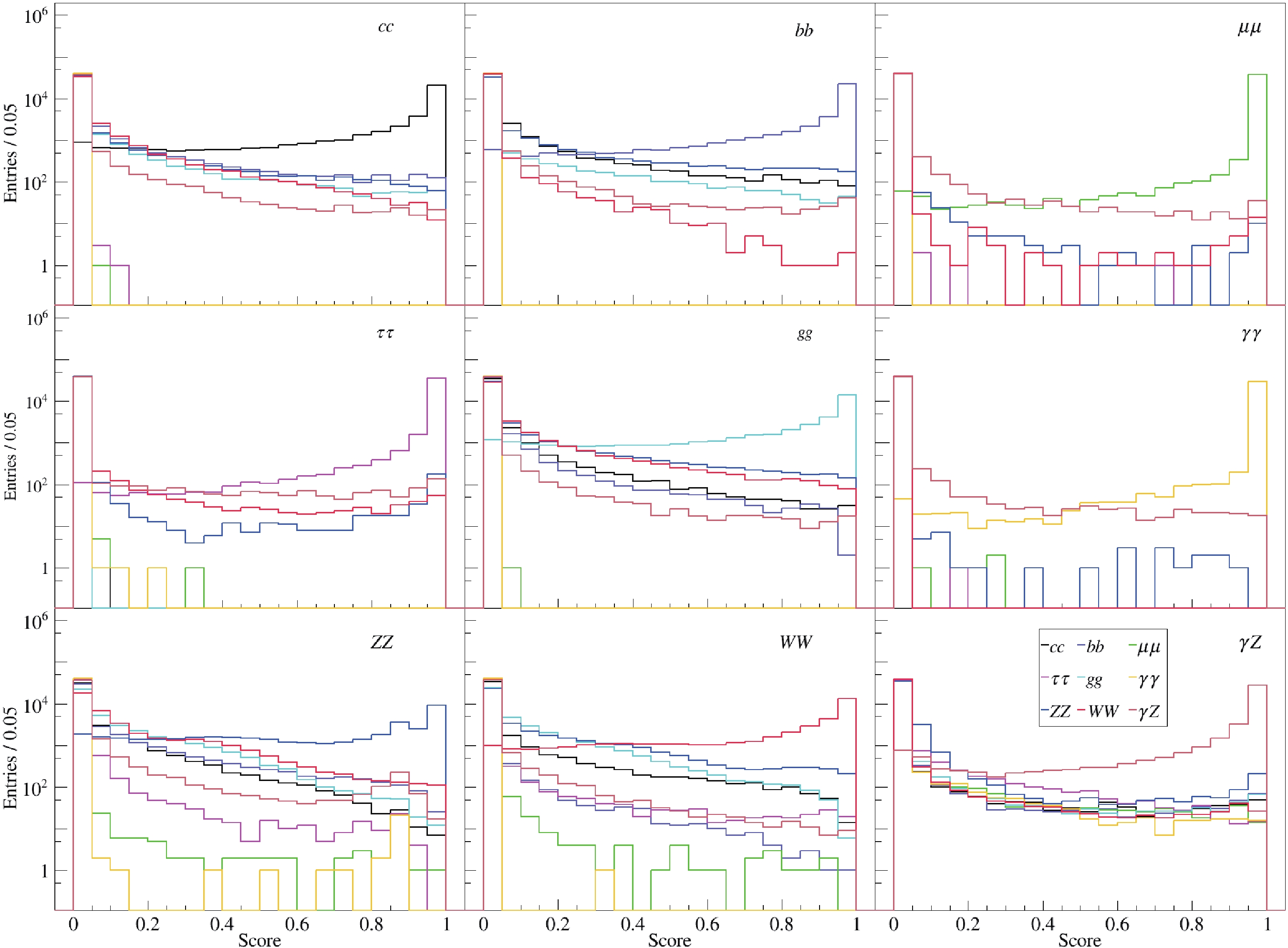
Figure 2. (color online) The distributions of 9 outputs for each true category, taking
$ e^+e^-H $ as an example. Each score is calculated by assuming that the event belongs to that category.
Figure 3. (color online) Classification performance on the test set visualized with t-SNE, where the two largest components are used, taking 10,000 events of
$ e^+e^-\to e^+e^-H $ for illustration.Some standard quantities can measure the performances of classifiers. For instance, efficiency (EFF) measures the fraction of correctly classified observations, ROC curve (Receiver Operating Characteristic curve) visualizes the True Positive Rate (TPR) versus the False Positive Rate (FPR), and AUC (Area Under the Curve) is the area under the ROC curve. If we have a better classification for each threshold value, the area grows, and a perfect classification leads to an AUC of 1.0. The EFF and AUC for all 36 processes in the 4 tagging modes are summarized in Table 2. Several conclusions can be drawn from the table. First, the accuracy reaches about 87%, which is good and adequate for further analysis. The decays of
$ H\to \mu^+\mu^- $ ,$ \tau^+\tau^- $ , and$ \gamma\gamma $ have the best efficiency and largest AUCs, as expected. Last but not least, the efficiencies of$ H\to ZZ^* $ or$ WW^* $ are not as good as the others. The main reason is that the similarities between them, as well as bits of$ bb $ ,$ cc $ , and$ gg $ can also fake$ WW^* $ /$ ZZ^* $ . This leaves room for further improvement.Decay mode $ e^+e^-H $ 

$ \mu^+\mu^- H $ 

$ \tau^+\tau^- H $ 

$ q\bar{q}H $ 

EFF AUC EFF AUC EFF AUC EFF AUC $ H\to c\bar{c} $ 

0.880 0.991 0.882 0.991 0.857 0.987 0.755 0.966 $ H\to b\bar{b} $ 

0.908 0.994 0.893 0.994 0.877 0.991 0.733 0.972 $ H\to \mu^+\mu^- $ 

0.997 1.000 0.986 1.000 0.981 1.000 0.983 1.000 $ H\to \tau^+\tau^- $ 

0.993 0.999 0.985 0.999 0.985 0.999 0.982 0.999 $ H\to gg $ 

0.810 0.985 0.830 0.986 0.816 0.982 0.736 0.954 $ H\to \gamma\gamma $ 

0.997 1.000 0.999 1.000 1.000 1.000 0.997 1.000 $ H\to ZZ^* $ 

0.650 0.958 0.667 0.960 0.585 0.947 0.535 0.926 $ H\to WW^* $ 

0.806 0.981 0.801 0.981 0.771 0.974 0.632 0.952 $ H\to \gamma Z $ 

0.921 0.996 0.936 0.996 0.910 0.993 0.896 0.993 Table 2. Efficiencies (left) and AUCs (right) of four classifiers.
Finally, the confusion matrices are used to evaluate the performance of the ML model and to be used as an important ingredient for further data analysis. Confusion matrices are calculated by comparing the prediction of the model and the true labels. Figure 4 shows the confusion matrices of the four classifiers. In terms of the confusion matrix, the efficiencies appear as the diagonal elements of the corresponding confusion matrices, and the off-diagonal elements represent misclassification rates. So confusion matrices contain complete information of both the correct and incorrect classifications, which could help to unfold the generated numbers of signals,
$ N_i $ .
Figure 4. (color online) Confusion matrices of (a):
$ e^+e^- \to e^+e^- H $ , (b):$ e^+e^- \to \mu^+\mu^-H $ , (c):$ e^+e^- \to \tau^+\tau^-H $ , and (d):$ e^+e^- \to q\bar{q}H $ . -
The above study shows that multicategory classification is very promising in data analysis, so here a more ambitious case of 39-category classification will be tried. For the signal processes, considering that Z decays into 4 categories (neglecting neutrino decay and W fusion processes up to now), i.e,
$ e^+e^- $ ,$ \mu^+\mu^- $ ,$ \tau^+\tau^- $ , and$ q\bar{q} $ , and that the Higgs has the same 9 decay modes as above, so there are 36 signals. For a realistic analysis, the backgrounds must be taken into account, especially the irreducible ones. In the analysis of$ e^+e^- \to ZH $ study, the irreducible backgrounds mainly come from the SM process of$ e^+e^- \to ZZ $ . The background can be categorized into 3 classes depending on the decays of Z bosons, i.e, pure leptonic ($ ZZ_{l} $ ), semi-leptonic($ ZZ_{sl} $ ), and hadronic ($ ZZ_{h} $ ) decays. Overall it is a 39-category classification problem.Same data sets of the signal and extra 3 background processes are pre-processed with the same procedure, which has 39
$ \times $ 400,000 = 15,600,000 events, which is very challenging because of memory usage. So we switch to another deep learning framework, ParticleNet/Weaver[27, 39], which has a more flexible memory strategy.The confusion matrix of the 39-category classification is presented in Fig. 5, which shows very good separation power among all 39 processes. For the signal, four blocks of the
$ e^+e^-H $ ,$ \mu^+\mu^-H $ ,$ \tau^+\tau^-H $ , and$ q\bar{q}H $ processes can be seen clearly, which demonstrate similar patterns to the corresponding processes in Fig. 4. In each sub-matrix, the$ H\to \gamma\gamma $ ,$ \mu^+\mu^- $ , and$ \tau^+\tau^- $ decays achieve the best performances. Among the four "blocks", the misclassification rates are rather small. The$ H\to ZZ^* $ decay doesn't achieve as good performance as the other decays, which is also consistent with the results of the 9-category classification. For the irreducible backgrounds of$ e^+e^- \to ZZ $ , all of three processes are labeled correctly with very high efficiencies, greater than 90%, which indicates that the kinematics of different events can be learnt to discriminate the irreducible backgrounds by the ParticleNet.
Figure 5. (color online) Confusion matrix of the 39-category classification.
In this 39-category classification, all 9 Higgs decays in 4 tagging modes with the irreducible backgrounds together can be classified with rather good accuracy. It is different to the single tagging mode, which indicates that the Higgs decays can be determined with a combined method using much more information.
-
In this paper, we presented a study of the classification of the Higgs decays with the state-of-the-art ML approaches at electron–positron colliders. We deploy the ML techniques and try to classify both the signal and background events with only particle-level information and to obtain the confusion matrices, which can be used in further data analysis. This approach is the basis of an efficient and balanced "one-stop" analysis, which makes it possible to measure all Higgs branching fractions using all detector information and taking all the commonalities and correlations into account. For the analyses of tens or hundreds of channels, they can be repeated using this technique in a few days if all data samples are ready. In contrast, the time could be considerably longer using conventional analysis methods.
This work is only a feasibility study. There are various possibilities to improve and further validate these methods. One is to enhance the performance by taking the sequential decays of W and Z bosons into account and add more categories in the classification, which can adopt more information for each category and enhance the classification performance. Another endeavor with more physical significance is incorporating some physics processes beyond the SM in the analysis, such as invisible and semi-invisible decays of the Higgs boson, which can enhance the sensitivity of an experiment to new physics. In addition, an important issue is to investigate the detailed performance of the classification method based on full simulation. It is also very constructive to take the full SM backgrounds and main systematic uncertainties into account.
-
The authors present special thanks to Yunxuan Song, Congqiao Li, Dr. Yu Bai, and Dr. Huilin Qu for useful discussion and advice. The authors thank the IHEP Computing Center for its firm support.
Classify the Higgs decays with the PFN and ParticleNet at electron–positron colliders
- Received Date: 2022-07-07
- Available Online: 2022-11-15
Abstract: Various Higgs factories are proposed to study the Higgs boson precisely and systematically in a model- independent way. In this study, the Particle Flow Network and ParticleNet techniques are used to classify the Higgs decays into multicategories, and the ultimate goal is to realize an "end-to-end" analysis. A Monte Carlo simulation study is performed to demonstrate the feasibility, and the performance looks rather promising. This result could be the basis of a "one-stop" analysis to measure all the branching fractions of the Higgs decays simultaneously.


 DownLoad: