


 Abstract
 HTML
HTML Reference
 Related
 PDF
PDF


-
The Standard Model (SM) [1, 2] of particle physics predicts the existence of one neutral scalar particle, known as the Higgs boson [3–5]. Electro-weak spontaneous symmetry breaking is introduced by the Higgs mechanism through a complex doublet scalar field. In 2012, the ATLAS [6] and CMS [7] Collaborations claimed the discovery of a new particle with a mass of approximately 125 GeV. Subsequent research has revealed that this particle is consistent with the predicted Higgs boson in the SM.
Interactions between the Higgs boson and third-generation charged fermions have been observed by both the ATLAS and CMS Collaborations [8–10], whereas Higgs couplings to other generations of fermions have not yet been observed. The
$ H\to\mu^+\mu^- $ process is important for probing the properties of Higgs Yukawa couplings to second generation fermions. Recently, in the ATLAS experiment, the detection significance of the$ H \rightarrow {{\mu^+\mu^-}} $ process was found to be 2.0$ \sigma $ (expected value of 1.7$ \sigma $ ) with$ pp $ collision data collected at$ \sqrt{s}=13 $ TeV with an integrated luminosity of 139 fb$ ^{-1} $ [11]. In the CMS experiment, the significance was 3.0$ \sigma $ (expected value of 2.5$ \sigma $ ) with an integrated luminosity of 137 fb$ ^{-1} $ [12]. In projections with the ATLAS detector at the HL-LHC (3000 fb$ ^{\rm{-1}} $ ), the expected precision of the branching ratio (BR) of$ H \rightarrow {{\mu^+\mu^-}} $ is 14% [13]. At the International Linear Collider (ILC), the combined precision of the BR ($ H \rightarrow {{\mu^+\mu^-}} $ ) is estimated to be 17% [14]. The relative uncertainty on the measurement of$ \sigma(ZH)\times B(H\to \mu\mu) $ from the expected Future Circular Collider electron-positron (FCC-ee) data is 19% with an integrated luminosity of 5 ab$ ^{-1} $ at$ \sqrt{s}=240 $ GeV [15].Similar to other lepton colliders, the Circular Electron Positron Collider (CEPC) [16] has significant advantages for Higgs boson property measurements. The signal-to-noise ratio (SNR) is significantly higher than that of other colliders owing to the lepton collisions. Moreover, Higgs boson candidates can be identified using the recoiled mass method without tagging its decay products. A previous study [17, 18] was performed with the CEPC detector at a center-of-mass energy of 250 GeV with an integrated luminosity of 5 ab
$ ^{-1} $ . The detection significance from a counting experiment was reported in a$ {{\mu^+\mu^-}} $ mass window of [124.3,125.2] GeV. According to the new design parameters of the CEPC experiment, the center-of-mass energy would be updated to 240 GeV and the integrated luminosity would be accumulated up to 5.6 ab$ ^{-1} $ over seven years [19]. The benchmark of the detector has been optimized from Pre-CDR [16] to CDR [19]. It is interesting and important to re-study the$ H\to\mu\mu $ process with the latest benchmark of the CEPC detector and the corresponding updated Monte Carlo (MC) samples. Event selections are updated and the Toolkit for Multivariate Data Analysis (TMVA) is applied to improve the sensitivity. The expected significance is estimated using the asymptotic approximation [20] method. Moreover, the performance of the CEPC detector is discussed by smearing the resolution of muon momentum in simulated events (Section VII).This paper is organized as follows. Section II briefly summarizes the CEPC detector and MC samples. Section III presents object reconstruction and event selection. In Section IV, we further optimize event categorization using the TMVA method. In Section V, we study the signal and background models. In Section VI, we calculate the expected measurement precision of the
$ H\to\mu^+\mu^- $ process in the CEPC experiment. Section VII contains discussions on the CEPC detector performance. Finally, Section VIII concludes the analysis. -
The baseline detector concept based on MC simulation studies at the CEPC is developed using the International Large Detector (ILD) through an optimization sequence [19]. The detector is composed of a high precision silicon based vertex and tracking system, Time Projection Chamber (TPC), silicon-tungsten sampling electromagnetic calorimeter (ECAL), resistive plate chamber (RPC)-steel sampling hadron calorimeter (HCAL), 3-Tesla solenoid, and muon/yoke system [21]. The center of mass energy (
$ \sqrt{s} $ ) of the$ e^{+}e^{-} $ collision for Higgs production is 240 GeV. A GEANT4-based detector simulation framework, MokkaPlus (an updated version of Mokka [22]), is used for the CEPC detector simulation. MC events at the CEPC are generated with the Whizard V1.9.5 [23] program at leading order (LO) with initial state radiation (ISR) effects [24] taken into account. Pythia 6 [25] is used for parton showering and hadronization with parameters tuned based on Large Electron Positron Collider (LEP) [26] data. The analysis focuses on the signal process$ e^{+}e^{-} \rightarrow Z(\to q\bar{q}) H(\to\mu^{+}\mu^{-}) $ , where the$ Z $ boson decays into two jets. There are two types of background components: the two-fermion background ($ e^{+}e^{-} \rightarrow f\bar{f} $ ) and four-fermion background. The four fermions in the final states can be combined into two bosons, which are$ Z $ or$ W $ , and the processes are known as "$ ZZ $ " and "$ WW $ ," respectively. Additionally, when the final states contain a pair of electrons and an accompanying neutrino, the process is excluded from the "$ ZZ $ " and "$ WW $ " groups and is refered to as "single$ Z $ " or "single$ W $ ," which indicates the origin of the two remaining fermions. If several final particles can originate from either "$ ZZ $ " or "$ WW $ ," for instance,$ \nu_{\mu}\bar{\nu_{\mu}}\mu^{+}\mu^{-} $ , they are known as a "$ ZZ $ or$ WW $ mix." An analogous combination can also occur between the "single$ Z $ " and "single$ W $ ," which will be referred to as "single$ Z $ or single$ W $ ." The "$ ZZ $ or$ WW $ mix" and "single$ Z $ or single$ W $ " processes are grouped as "$ Z $ or$ W $ " background. For completeness, all background MCs are used in the analysis, although it can be expected that most background will be excluded after event selection (Section III) in the$ Z(\to q\bar{q})H(\to\mu^{+}\mu^{-}) $ phase space, where there are two muons and two jets in the final states. The dominant background in the analysis is the "$ ZZ $ " process, where one of the$ Z $ bosons decays into two muons and the other decays into two quarks.Table 1 summarizes the cross sections and statistics of the MC samples used in the analysis. The signal sample is produced with the Higgs mass at 125 GeV. The designed integrated luminosity of the collected Higgs events from the CEPC detector is 5.6 ab
$ ^{-1} $ . To normalize the simulated events to the expected yields of 5.6 ab$ ^{-1} $ , scale factors are applied and shown in the table.Process $ Z(\to q\bar{q})H(\to{{\mu^+\mu^-}}) $ 

Single $ Z $ 

Single $ W $ 

$ WW $ 

$ ZZ $ 

$ Z $ or

$ W $ 

2 $ f $ 

$ \sigma $ [fb]

0.02977 1541.68 3485.25 9076.11 1140.97 3899.63 143180.71 Statistics $ \sim $ 100 k

$ \sim $ 8 M

$ \sim $ 18 M

$ \sim $ 50 M

$ \sim $ 6 M

$ \sim $ 20 M

$ \sim $ 30 M

Norm Factor 0.0017 1.1 1.1 1.1 1.1 1.1 27 Table 1. Cross sections and statistics of the simulated MC samples. To normalize the simulated events to the expected yields of 5.6 ab
$ ^{-1} $ , scale factors are applied. -
A dedicated particle flow reconstruction toolkit, ARBOR [27, 28], has been developed for the CEPC baseline detector concept [19]. The matching module inside ARBOR identifies calorimeter clusters with matching tracks and builds reconstructed charged particles. In particle flow reconstruction, muons exhibit themselves as minimum ionizing particles in the calorimeter matched with tracks in the tracker as well as in the muon detector. A lepton identification algorithm, LICH [29], has been developed and implemented in ARBOR. LICH combines discriminating variables to build lepton-likelihoods using a multivariate technique. The momenta of muons are determined by their track momenta. The particle flow algorithm provides a coherent interpretation of an entire physics event and is therefore well suited for the reconstruction of compound physics objects, such as jets, which are formed from particles reconstructed by ARBOR using the Durham clustering algorithm (
$ e^{+}e^{-} $ $ k_{T} $ -algorithm) [30]. Jet energies are calibrated through a two-step process. First, calibrations are applied to particles identified by ARBOR. In the second step, the jet energies are calibrated using physics events. At the CEPC,$ W $ and$ Z $ bosons are copiously produced and can be identified with high efficiency and purity. Thus, the$ W\to q\bar{q} $ and$ Z\to q\bar{q} $ decays serve as standard candles for jet energy calibration. The large statistics allows the jet response to be characterized in detail. Specifically, in the analysis, only muons with momenta greater than 30 GeV are considered. Two muons with different charges are selected with the closest invariant mass to the Higgs boson mass (125 GeV). The signal process focuses on the hadronic decay of the$ Z $ boson ($ Z \rightarrow q\bar{q} $ ) owing to its large branching fraction. After excluding the selected$ \mu^+ $ and$ \mu^- $ , the Durham algorithm reconstructs all remaining particles into two jets.Event selection is optimized to improve the signal significance. This analysis requires at least two muons with opposite signs. The Higgs boson candidate is selected by requiring
$ |m_{\mu\mu}-m_{H}|<10 $ GeV, where$ m_{H}=125 $ GeV. Owing to the signature topology of two jets in the final state, the number of reconstructed particles should be greater than the leptonic final states, which must be greater than 25 and less than 115. The di-jet invariant mass is similar to the$ Z $ boson mass, which is selected to be greater than 55 GeV and less than 125 GeV. The four-momentum of the$ q\bar{q}{{\mu^+\mu^-}} $ system should be close to (0, 0, 0,$ \sqrt{s} $ ). Therefore, the momemtum of the$ q\bar{q}{{\mu^+\mu^-}} $ system is less than 32 GeV, and the energy is greater than 195 GeV and less than 265 GeV. To supress contamination from the$ WW $ background, the energy of the muon is required to be greater than 35 GeV and less than 100 GeV. The momenta of the missing energies must be less than 20 GeV along both the$ x $ - and$ y $ -axes, and the solid angle between the$ q\bar{q}\mu $ system and the other muon must be greater than 2.5 rad. To supress contamination from the hadronic background, the momentum of the di-muon system must be greater than 18 GeV and less than 72 GeV.After these selections, the signal efficiency is 77%. The dominant background is the
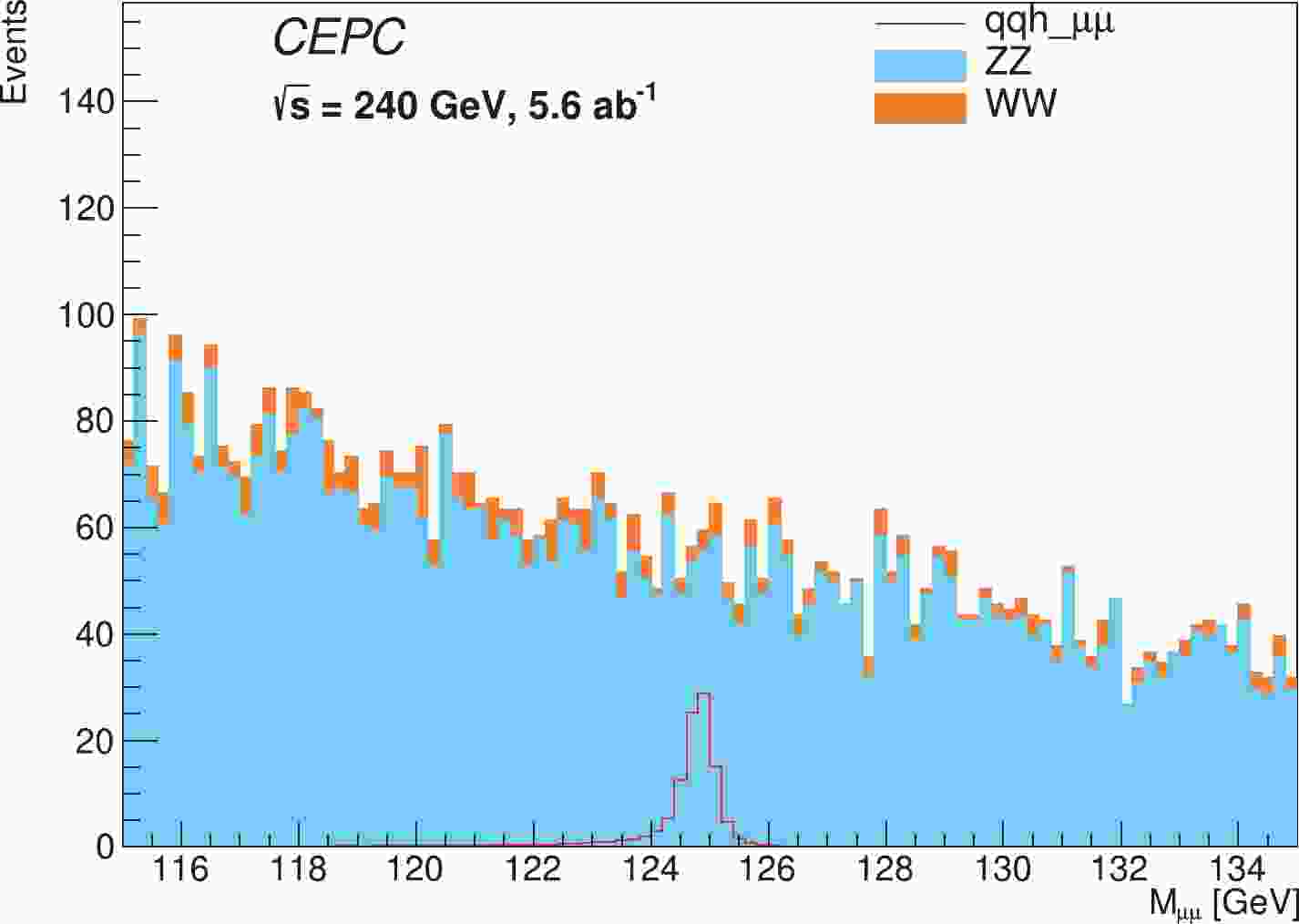
$ ZZ $ process decaying into a di-muon and di-jet, which accounts for 93% of the total background. The remaining background is the$ WW $ process. Contributions from other background processes are found to be negligible. The signal region is defined as$ 115<m_{{{\mu^+\mu^-}}}<135 $ GeV. Fig. 1 shows the$ {{\mu^+\mu^-}} $ invariant mass distributions of the signal and background events after event selection. The red curve is the$ Z(\to q\bar{q})H(\to{{\mu^+\mu^-}}) $ signal. The azure histogram is the$ ZZ $ background, and the orange histogram is the$ WW $ background. The signal detection significance through a counting experiment (counting significance) is defined as$ Z=\sqrt{2[(S+B)\ln(1+\frac{S}{B})-S]} $ , where$ S $ and$ B $ are the corresponding signal and background yields in the$ {{\mu^+\mu^-}} $ mass region of [124.1,125.5] GeV, respectively, which is triple the resolution of the signal model fitted by the Double Sided Crystal Ball function (DSCB, see Section V). The significance is estimated to be 4.9$ \sigma $ .
Figure 1. (color online)
$ {{\mu^+\mu^-}} $ invariant mass distributions of the signal and background events after event selection. The red curve is the$ Z(\to q\bar{q})H(\to{{\mu^+\mu^-}}) $ signal. The azure histogram is the$ ZZ $ background, and the orange histogram is the$ WW $ background. -
TMVA technology is applied to categorize events for further optimization of the signal significance. The gradient boosted decision trees (BDTG) method is used in the analysis. After event selection, nine discriminant variables are used for Multivariate Data Analysis (MVA) training to separate the signal and background processes:
$ \cos\theta_{q\bar{q}} $ ,$ m_{q\bar{q}} $ ,$ \Delta_{q2,\mu^+} $ ($ \Delta $ and$ q1/q2 $ represent the solid angle and leading/sub-leading jet, respectively),$ \Delta_{q1,\mu^-} $ ,$ p_{x}^{q2} $ ,$ p_{y}^{q2} $ ,$ \Delta_{\mu^-,\mu^+} $ ,$ \cos\theta_{q2} $ , and$ \cos\theta^{*}_{\mu^{+},\mu^{-}} $ ①. The signal and background distributions of these variables are shown in Fig. 3. The red curve is the$ Z(\to q\bar{q})H(\to{{\mu^+\mu^-}}) $ signal. The azure histogram is the$ ZZ $ background, and the orange histogram is the$ WW $ background. In Fig. 3, the backgrounds are normalized to the corresponding cross sections multiplied by the integrated luminosity accounting for selection efficiencies. The signal yield is scaled to the total background yield.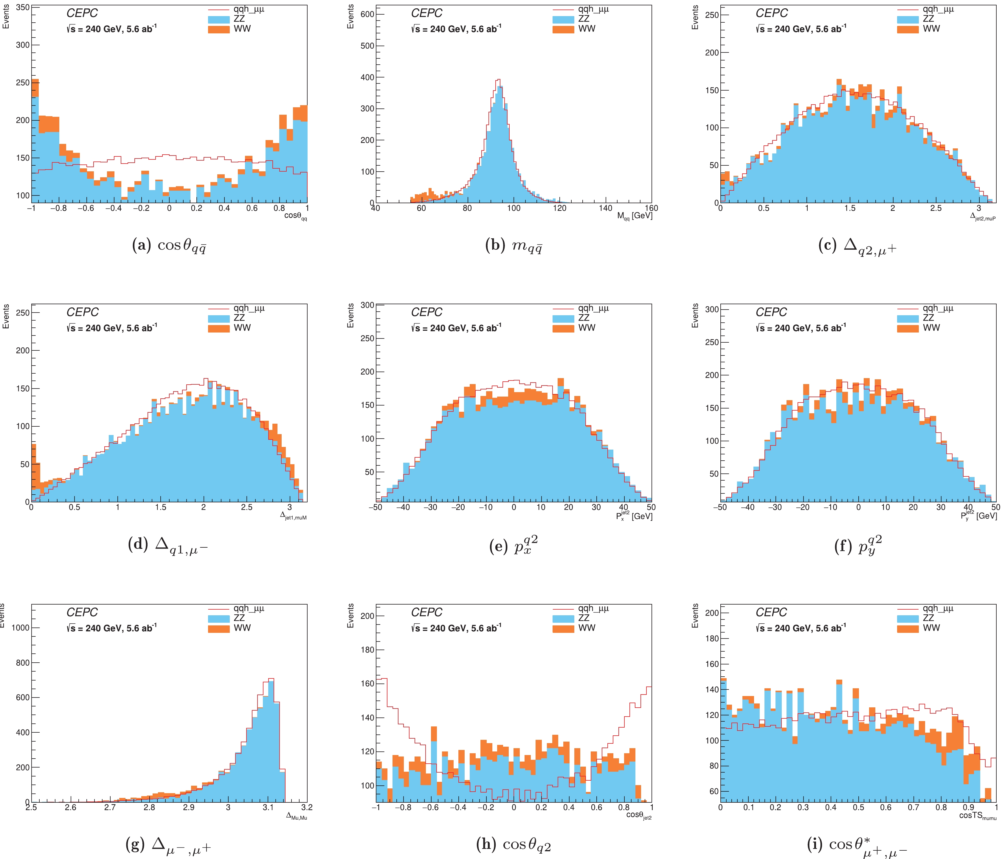
Figure 3. (color online) Signal and background distributions of nine discriminant variables. The red curve is the
$ Z(\to q\bar{q})H(\to{{\mu^+\mu^-}}) $ signal. The azure histogram is the$ ZZ $ background, and the orange histogram is the$ WW $ background. Backgrounds are normalized to the corresponding cross sections multiplied by the integrated luminosity. The signal yield is scaled to the background yield.The events are equally divided into training and test subsets. The training events are trained using the BDTG method to classify the signal and background with an output discriminating variable constructed from nine input variables. To reduce potential over-training effects, only test events are used to evaluate the goodness of the signal and background classification. The BDTG distribution of the total events is shown in Fig. 2. The signal significance is estimated as a function of BDTG response to find the optimal cut to classify two event categories, where the greatest total counting significance (
$Z_{\rm total}= \sqrt{Z_{1}^{2}+Z_{2}^{2}}$ ) is obtained. As a result, tight (BDTG > 0.01) and loose (BDTG < 0.01) categories are defined. Fig. 4 shows$ m_{{{\mu^+\mu^-}}} $ distributions in the tight (a) and loose (b) categories. The combined counting significance is estimated to be 5.6$ \sigma $ , with a 14% improvement with respect to the inclusive significance (4.9$ \sigma $ ). The tight category contributes the most to the sensitivity with a significance of 5.2$ \sigma $ . The event yields of the signal and background components in each category are summarized in Table 2, where the signal and background yields are normalized to the corresponding cross sections multiplied by an integrated luminosity of 5.6 ab$ ^{-1} $ .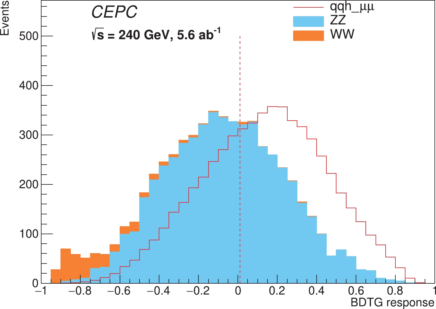
Figure 2. (color online) BDTG reponse after training. The red curve is the
$ Z(\to q\bar{q})H(\to{{\mu^+\mu^-}}) $ signal. The azure histogram is the$ ZZ $ background, and the orange histogram is the$ WW $ background. The signal yield is scaled to the background yield.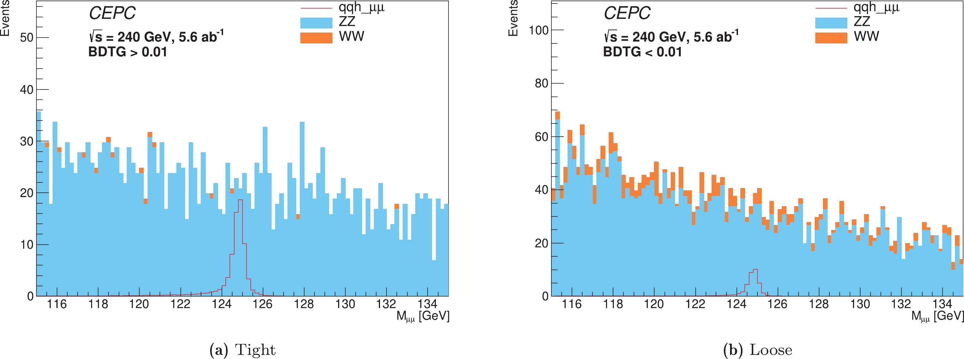
Figure 4. (color online)
$ m_{{{\mu^+\mu^-}}} $ distributions in the tight (a) and loose (b) categories. The azure histogram is the$ ZZ $ background, and the orange histogram is the$ WW $ background.Category $Z(\to q\bar{q})H(\to{{\mu^+\mu^-}})$ 

$WW$ 

$ZZ$ 

Tight 84.50 16 2461 Loose 44.25 386 3590 Total 128.75 402 6051 Table 2. Event yields of the signal and background components in each category.
-
The observable of the analysis is
$ m_{{{\mu^+\mu^-}}} $ because the di-muon final state can be fully reconstructed with excellent efficiency. The narrow resonance rising above a smooth background in the$ m_{{{\mu^+\mu^-}}} $ distribution can be used to extract the Higgs boson signal with good mass resolution. The signal model is described by the DSCB.$ f(t)=N\times \left\{ \begin{array}{*{20}{l}} {\rm e}^{-\frac{1}{2}t^{2}},& -\alpha_{L}\le t\le\alpha_{H}\\ {\rm e}^{-\frac{1}{2}\alpha_{L}^{2}}\left[\dfrac{\alpha_{L}}{n_{L}}\left(\dfrac{n_{L}}{\alpha_{L}}-\alpha_{L}-t\right)\right]^{-n_{L}},& t<-\alpha_{L}\\ {\rm e}^{-\frac{1}{2}\alpha_{H}^{2}}\left[\dfrac{\alpha_{H}}{n_{H}}\left(\dfrac{n_{H}}{\alpha_{H}}-\alpha_{H}+t\right)\right]^{-n_{H}},& t>\alpha_{H}. \end{array} \right. $

(1) Here,
$ t=(m_{{{\mu^+\mu^-}}}-\mu_{CB})/\sigma_{CB} $ . Fig. 5 shows the$ m_{{{\mu^+\mu^-}}} $ distributions of the signal process and the fitted DSCB curves of the two categories. The DSCB can describe the signal$ m_{{{\mu^+\mu^-}}} $ distribution very well. The$ \mu_{CB} $ is estimated to be$ 124.83 $ GeV ($ 124.82 $ GeV) in the tight (loose) category, and the resolution ($ \sigma_{CB} $ ) is estimated to be$ 0.23 $ GeV ($ 0.22 $ GeV) for the tight (loose) category.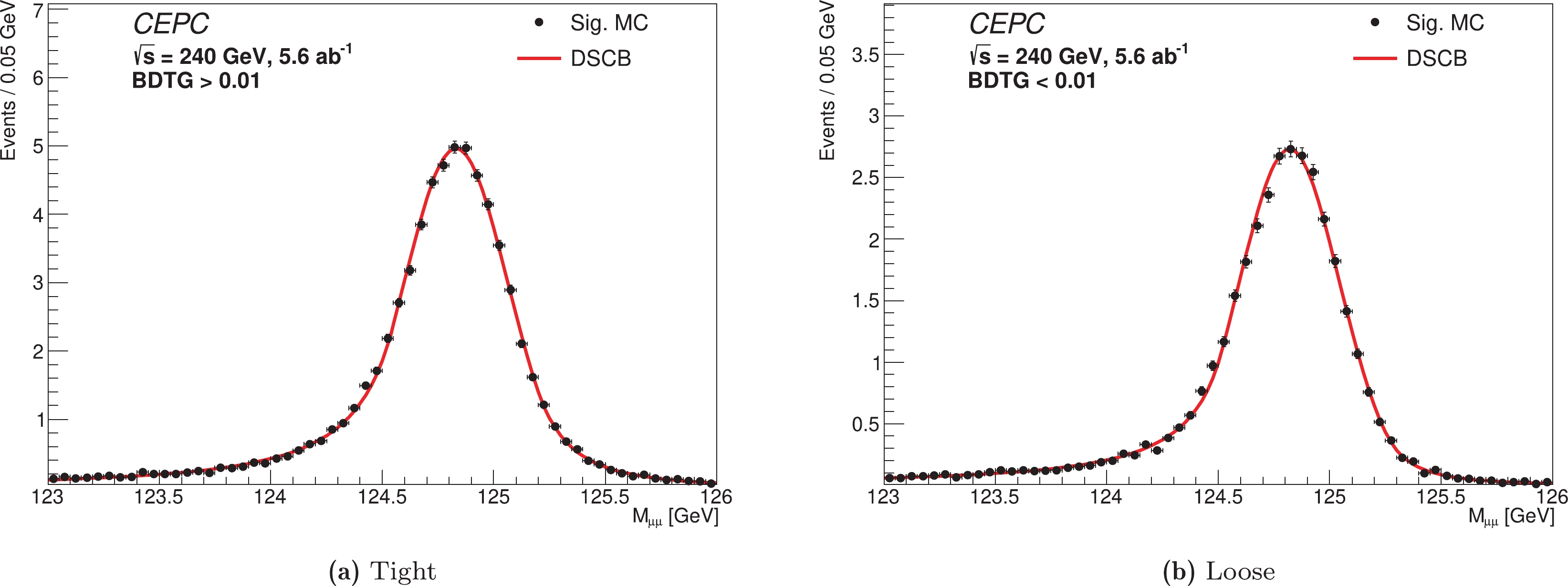
Figure 5. (color online)
$ m_{{{\mu^+\mu^-}}} $ distribution of the signal process and the fitted DSCB curve in the tight (a) and loose (b) categories.Several background functions (for example, Chebyshev polynomials, exponential functions, and polynomials) are employed to fit the background mass distributions, and the second-order Chebyshev function is finally selected owing to the minimum
$ \chi^{2} $ obtained in the fits. This function is described as$ \begin{array}{l} f(m_{{{\mu^+\mu^-}}})=N\times[1+a_{0}m_{{{\mu^+\mu^-}}}+a_{1}(2m_{{{\mu^+\mu^-}}}^{2}-1)]. \end{array} $

(2) Fig. 6 shows the background MC mass distributions and fitted results in the two categories.
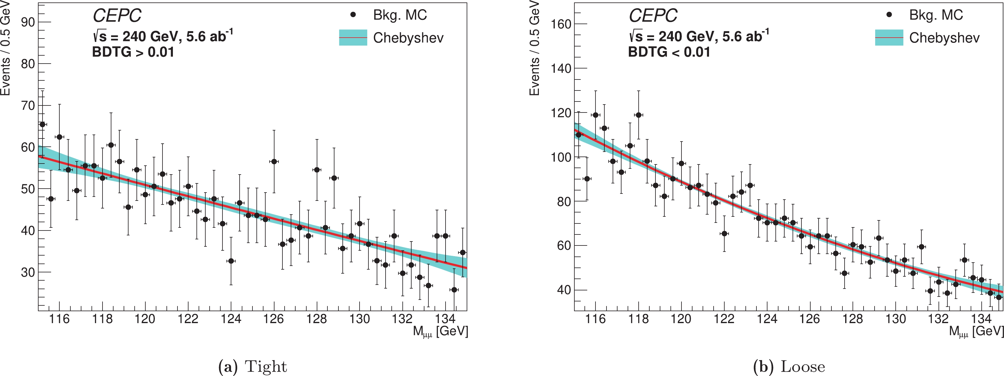
Figure 6. (color online)
$ m_{{{\mu^+\mu^-}}} $ distribution of the background processes and the fitted result in the tight (a) and loose (b) categories. -
In the statistical analysis, pseudo-data are employed to mimic the real
$ m_{{{\mu^+\mu^-}}} $ distribution of the observed data collected by the CEPC detector, which is constructed by combining the signal and background MC events. The expected signal events are extracted from the pseudo-data via fitting on the$ m_{{{\mu^+\mu^-}}} $ distribution in the two categories simultaneously. The unbinned maximum likelihood method is used, and the fitting range is [115,135] GeV. The likelihood function is defined as$ \begin{aligned}[b] {\cal{L}}\left(m_{{{\mu^+\mu^-}}}\right)=&\prod\limits_{c}\bigg(\operatorname{Pois}(N \mid \mu S+B)\cdot\\ & \prod\limits_{n=1}^{N} \frac{\mu S \times f_{S}\left(m_{{{\mu^+\mu^-}}}\right)+B \times f_{B}\left(m_{{{\mu^+\mu^-}}}\right)}{\mu S+B}\bigg), \end{aligned} $

(3) where
$ N $ is the pseudo event number in category$ c $ , and the signal strength is defined as the ratio of the measured signal yield to that expected in the SM:$ \begin{aligned}[b]\mu=\dfrac{N(e^{+}e^{-}\to Z(\to q\bar{q})H(\to{{\mu^+\mu^-}}))}{N^{\rm SM}(e^{+}e^{-}\to Z(\to q\bar{q})H(\to{{\mu^+\mu^-}}))}\end{aligned} $

which is the parameter of interest (POI) in this analysis.
$ S $ and$ B $ are the expected signal and background events, respectively, in category$ c $ , and$ f_{S} $ and$ f_{B} $ are the signal and background models, respectively, in category$ c $ . For the fitting, the signal model parameters are fixed to those in the fitting of the signal MC, and the background model parameters are floated.In the analysis, to avoid statistical fluctuations in the MC samples, Asimov data [20] are generated and fitted to obtain the expected precision and significance of the signal process. Fig. 7 shows the
$ m_{{{\mu^+\mu^-}}} $ distribution of the Asimov data and the fitted models in the two categories. The blue curve is the fitted signal + background model, the red curve is the signal component, and the dashed blue curve is the background component. The expected signal strength$ \mu $ is estimated to be$ 1.00_{-0.18}^{+0.19} $ with statistical uncertainty. The corresponding significance is 6.1$ \sigma $ . To estimate the potential over-training effects on the background events during BDTG event categorization (Section IV), the background categorization efficiency uncertainty accounting for the difference between the training and test background events is applied. The statistical uncertainties on the background model parameters ($ a_{0} $ and$ a_{1} $ of Formula (2)), which are calculated via fitting on the background MC samples, are applied as well as the background shape uncertainties. It is found that the above systematic impacts on the$ H\to\mu^{+}\mu^{-} $ signal measurement precision and significance are negligible and are thus neglected in the study.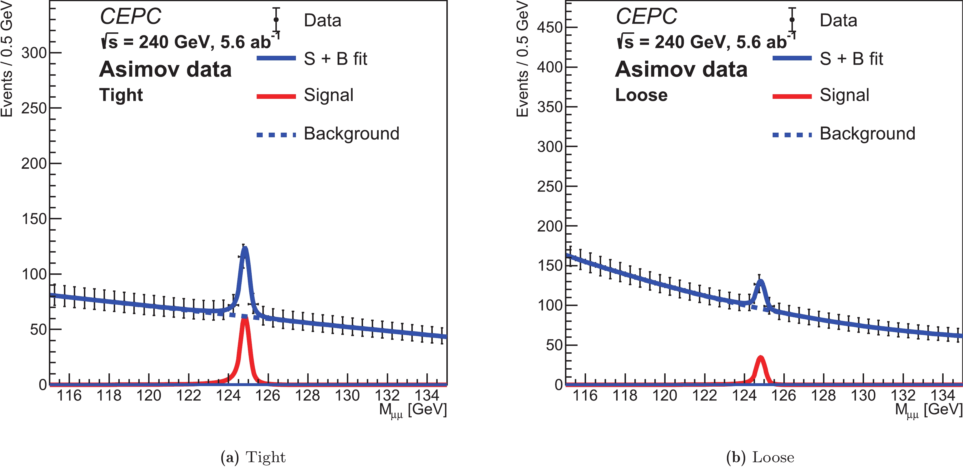
Figure 7. (color online)
$ m_{{{\mu^+\mu^-}}} $ distribution of the Asimov data and the fitted models in the tight (a) and loose (b) categories. The blue curve is the fitted signal + background model, the red curve is the signal component, and the dashed blue curve is the background component.The High Luminosity Large Hadron Collider (HL-LHC) is an upgrade of the LHC that aims to collect
$ pp $ collision data with an integrated luminosity of 3000 fb$ ^{-1} $ at$ \sqrt{s}=14 $ TeV. The expected precision of the$ H\to\mu\mu $ measurement in the ATLAS experiment is extrapolated from the analysis using 79.8 fb$ ^{-1} $ of data at$ \sqrt{s}=13 $ TeV [13]. Approximately 41k$ pp\to H\to\mu\mu $ events will be generated at the HL-LHC, and the precision in the extrapolation is estimated to be 14%, whereas$ \sim $ 167$ e^{+}e^{-}\to Z(\to q\bar{q})H(\to\mu\mu) $ events are expected to be generated at the CEPC. With the help of the extremely high efficiency of muon events and clean backgrounds, the precision is of the same level for the two analyses. The prospects of measuring the branching fraction of$ H\to\mu\mu $ at the ILC have been evaluated considering centre-of-mass energies ($ \sqrt{s} $ ) of 250 GeV and 500 GeV [14]. For both$ \sqrt{s} $ cases, two final states,$ e^{+}e^{-}\to q\bar{q}H $ and$ e^{+}e^{-}\to \nu\bar{\nu}H $ , have been analyzed. For integrated luminosities of 2 ab$ ^{-1} $ at$ \sqrt{s}=250 $ GeV and 4 ab$ ^{-1} $ at$ \sqrt{s}=500 $ GeV, both the$ ZH $ and$ WW $ fusion production modes are considered, and$ \sim $ 199 signal events will be generated. The combined precision is estimated to be 17%. In the FCC-ee experiment [15], the expected uncertainty of$ \sigma(e^{+}e^{-}\to ZH)\times BR(H\to\mu\mu) $ is measured using 5 ab$ ^{-1} $ of data at$ \sqrt{s}=240 $ GeV. The 19% precision is compatible with the result estimated in the CEPC experiment. -
To study the CEPC detector performance on muon measurements, the resolution of the muon momentum (
$\sigma_{\mu}=(p_{\mu}^{\rm reco}-p_{\mu}^{\rm truth})$ ) is smeared by 25%, 50%, and 100%. The$ H\to{{\mu^+\mu^-}} $ measurement is repeated to estimate the reduction in the signal precision. The nominal momentum resolution of a muon is shown in Fig. 8(a), with the MC events (signal + background) passing all selections. The DSCB function is used to fit the spectrum, and$ \sigma_{CB} $ is measured to be 131 MeV.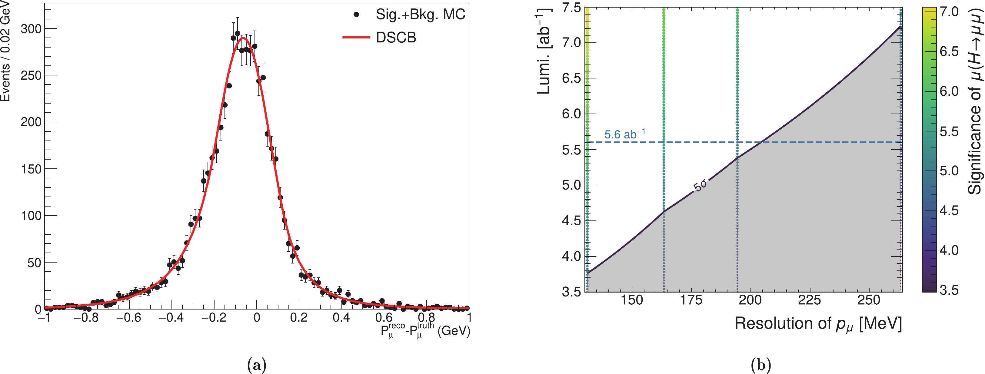
Figure 8. (color online) (a) Nominal momentum resolution of a muon with the signal MC events passing all selections. The DSCB function is used to fit the spectrum, and
$ \sigma_{CB} $ is measured to be 131 MeV. (b) Two dimensional expected significance of the$ H\to\mu\mu $ process as a function of the integrated luminosity and the momentum resolution of the muon. Colored scatters are the expected significances. Significances with the same momentum resolution, other than the measured numbers (Table 3) at the nominal integrated luminosity (5.6 ab$ ^{-1} $ ), are scaled by$ \sqrt{\frac{{\cal{L}}}{{\cal{L}}_{0}}} $ , where$ {\cal{L}} $ is the target integrated luminosity, and$ {\cal{L}}_{0} $ is the nominal one. It is assumed that the significance is only restricted by the number of events. The discovery curve is extrapolated with points in (resolution, integrated luminosity) space, and the expected significances in the gray band are below 5$ \sigma $ .Table 3 shows the expected signal strengths
$ \mu $ , significances, and reductions in significances by smearing the resolution of the muon momentum. The expected significances of the$ H\to\mu\mu $ process are shown in the two dimensional map of the integrated luminosity and the momentum resolution of the muon (Fig. 8 (b)). The colored scatters are the expected significances. Significances with the same momentum resolution, other than the measured numbers (Table 3) at the nominal integrated luminosity (5.6 ab$ ^{-1} $ ), are scaled by$ \sqrt{\frac{{\cal{L}}}{{\cal{L}}_{0}}} $ , where$ {\cal{L}} $ is the target integrated luminosity, and$ {\cal{L}}_{0} $ is the nominal one. It is assumed that the significance is only restricted by the number of events. The discovery curve is extrapolated with points in (resolution, integrated luminosity) space, and the expected significances in the gray band are below 5$ \sigma $ . The resolution must be better than 204 MeV to discover the$ H\to\mu\mu $ process at the nominal integrated luminosity. With the nominal muon momentum resolution of the detector, the integrated luminosity should be greater than 3.8 ab$ ^{-1} $ for the discovery of the di-muon process. In the worst case in which the resolution is 100% worse than the designed parameters, the integrated luminosity should be greater than 7.2 ab$ ^{-1} $ .Smearing 25% 50% 100% $ \mu $ 

$ 1.00_{-0.20}^{+0.21} $ 

$ 1.00_{-0.21}^{+0.22} $ 

$ 1.00_{-0.24}^{+0.25} $ 

Significance $ 5.5 \sigma $ 

$ 5.1 \sigma $ 

$ 4.4 \sigma $ 

Reduction in significance 10% 16% 28% Table 3. Expected signal strength
$ \mu $ , significance, and reduction in significance with the resolution of the muon momentum smeared by 25%, 50%, and 100%. -
The
$ e^{+}e^{-} \rightarrow Z(\to q\bar{q})H(\to\mu^{+}\mu^{-}) $ process is studied using MC events in the CEPC experiment. The simulated samples are generated with a center of mass energy of 240 GeV. Event selection is updated, and categorization is optimized using the BDTG method to improve the signal significance. The maximum unbinned likelihood fit method is applied and fitted on the Asimov$ m_{{{\mu^+\mu^-}}} $ distributions in two event categories simultaneously. With a designed integrated luminosity of 5.6 ab$ ^{-1} $ , the statistical-only precision of the expected signal is 19%, and the corresponding significance is 6.1$ \sigma $ . The systematic uncertainties from the background MC statistical fluctuations are evaluated and revealed to have a negligible impact on the$ H\to\mu^{+}\mu^{-} $ signal. The performance of the CEPC detector is further studied by smearing the resolution of the muon momentum by 25%, 50%, and 100% in the simulated MC samples. The impacts on the signal precision of this analysis are estimated. The resolution must be better than 204 MeV to discover the$ H\to\mu\mu $ process at the nominal integrated luminosity. If the resolution is 100% worse than the designed parameters, the integrated luminosity should be greater than 7.2 ab$ ^{-1} $ for this discovery.
Expected ${\boldsymbol H \xrightarrow{} {\boldsymbol{\mu^+\mu^-}}} $ measurement precision with ${\boldsymbol { e^{+}e^{-}}{\bf \xrightarrow{}}{ \boldsymbol{Z(q\bar{q})H}}}$ production at the CEPC
- Received Date: 2021-12-16
- Available Online: 2022-09-15
Abstract: A search for the dimuon decay of the Standard Model Higgs boson is performed using Monte Carlo simulated events to mimic data corresponding to an integrated luminosity of 5.6 ab


 DownLoad: