


 Abstract
 HTML
HTML Reference
 Related
 PDF
PDF


-
The decays of hadrons involving the flavor changing neutral current (FCNC) transition such as
$ \Lambda_b \rightarrow \Lambda l^+ l^- $ can provide essential information about the inner structure of hadrons, reveal the nature of the electroweak interaction, and provide model-independent information about physical quantities such as Cabibbo-Kobayashi-Maskawa (CKM) matrix elements. The rare decay$ \Lambda_b \rightarrow \Lambda \mu^+ \mu^- $ was first observed by the CDF collaboration in 2011 [1]. Some experimental progress on$ \Lambda_b \rightarrow \Lambda l^+ l^- $ was also achieved [2–5], and the radiative decay$ \Lambda_b \rightarrow \Lambda \gamma $ was observed in 2019 [3] by the LHCb collaboration. The LHCb collaboration determined the forward-backward asymmetries ($ A^l_{\rm FB} $ ) of the decay$ \Lambda_b \rightarrow \Lambda \mu^+ \mu^- $ to be$ {A}^l_{\rm FB}(\Lambda_b \rightarrow \Lambda \mu^+ \mu^-)= -0.05\pm 0.09 $ (stat)$ \pm0.03 $ (syst),$ {A}^h_{\rm FB}(\Lambda_b \rightarrow \Lambda \mu^+ \mu^-)=-0.29\pm0.09 $ (stat)$ \pm0.03 $ (syst), and$ F_{\rm L}(\Lambda_b \rightarrow \Lambda \mu^+ \mu^-)=0.61^{+0.11}_{-0.14} \pm 0.03 $ (syst) at the low dimuon invariant mass squared range$ 15 < q^2<20 $ GeV$ ^2 $ in 2015 [4]. However, these numbers were updated in 2018 to$ \bar{A}^l_{\rm FB}(\Lambda_b \rightarrow \Lambda \mu^+ \mu^-)=-0.39\pm 0.04 $ (stat)$ \pm0.01 $ (syst),$ {A}^h_{\rm FB}(\Lambda_b \rightarrow \Lambda \mu^+ \mu^-)=-0.3\pm0.05 $ (stat)$ \pm0.02 $ (syst), and$ \bar{A}^{lh}_{\rm FB}(\Lambda_b \rightarrow \Lambda \mu^+ \mu^-)=0.25\pm0.04 $ (stat)$ \pm0.01 $ (syst) in the same invariant mass squared region [5]. Note that$ A^l_{\rm FB} $ is significantly lager than the previous one. In this study, we investigate the$ A _{\rm FB} $ of$ \Lambda_b \rightarrow \Lambda l^+ l^- $ in the Bethe-Salpeter equation (BSE) approach. Theoretically, only a few studies have been conducted on$ {A}_{\rm FB}(\Lambda_b\rightarrow \Lambda l^+ l^-) $ [6–17]. References [6] ([7]) provided the integrated forward-backward asymmetries$ \bar{A}^l_{\rm FB}(\Lambda_b\rightarrow \Lambda \mu^+ \mu^-)= -0.13 $ ($ -0.12 $ ) and$ \bar{A}_{\rm FB}(\Lambda_b\rightarrow \Lambda \tau^+ \tau^-)=-0.04 $ ($ -0.03 $ ), whereas the results of Ref. [8] were$ \bar{A}^l_{\rm FB}(\Lambda_b\rightarrow \Lambda e^+ e^-)=1.2 \times 10^{-8} $ ,$ \bar{A}^l_{\rm FB}(\Lambda_b\rightarrow \Lambda \mu^+ \mu^-)= 8 \times 10^{-4} $ , and$ \bar{A}^l_{\rm FB}(\Lambda_b\rightarrow \Lambda \tau^+ \tau^-)= 9.6\times 10^{-4} $ . Ref. [10] analyzed the differential$ \bar{A}_{\rm FB}(\Lambda_b\rightarrow \Lambda l^+ l^-) $ in the heavy quark limit. Using the nonrelativistic quark model, Ref. [11] investigated the lepton-side forward-backward asymmetries$ \bar{A}^l_{\rm FB}(\Lambda_b\rightarrow \Lambda l^+ l^-) $ . In the quark-diquark model, Ref. [12] investigated the lepton-side forward-backward asymmetries$ A_{\rm FB} $ , the hadron-side forward-backward asymmetries$ A_{\rm FB}^h $ , and the hadron-lepton forward-backward asymmetries$ A^{hl}_{\rm FB} $ . In an approach of the light-cone sum rules, Refs. [13, 14] investigated the rare decays of$ \Lambda_b \rightarrow \Lambda \gamma $ and$ \Lambda_b \rightarrow \Lambda l^+ l^- $ . Ref. [15] investigated the phenomenological potential of the rare decay$ \Lambda_b \rightarrow \Lambda l^+ l^- $ with a subsequent, self-analyzing$ \Lambda_b \rightarrow N \pi $ transition. With the form factors (FFs) extracted from a constituent quark model, Ref. [16] investigated the rare weak dileptonic decays of the$ \Lambda_b $ baryon. Ref. [17] studied$ {\cal B}_1 \rightarrow {\cal B}_2 l^+ l^- $ ($ {\cal B}_{1,2} $ are spin$ 1/2 $ baryons) with the SU(3) flavor symmetry. The FFs of$ \Lambda_b \rightarrow \Lambda $ differ in different models. Generally, the number of independent FFs of$ \Lambda_b \rightarrow \Lambda $ can be reduced to 2 when working in the heavy quark limit [18],$ \begin{array}{*{20}{l}} \langle \Lambda(p)| \bar{s} \Gamma b | \Lambda_b(v) \rangle = \bar{u}_{\Lambda} (F_1(q^2) +F_2 (q^2) \not{v} )\Gamma u_{\Lambda_b}(v), \end{array} $

(1) where
$ \Gamma= \gamma_\mu,\; \gamma_\mu \gamma_5,\; q^\nu \sigma_{\nu\mu} $ , and$ q^\nu \sigma_{\nu\mu}\gamma_5 $ ,$ q^2 $ is the square of the transformed momentum. The FF ratio$ R(q^2)= F_2(q^2)/F_1(q^2) $ was considered a constant in many studies assuming the same shape for$ F_1 $ and$ F_2 $ , and it was derived from quantum chromodynamics (QCD) sum rules in the framework of the heavy quark effective theory [6]. For example, in Refs. [6, 7] the$ q^2 $ dependence of FF$ F_i\; (i=1,2) $ were given as follows:$ F_i(q^2) = \frac{F_i(0)}{1-a q^2+b q^4}, $

(2) where a and b are constants. Using experimental data for the semileptonic decay
$ \Lambda_c \rightarrow \Lambda e^+ \nu_e $ ($ m^2_{\Lambda} \leq q^2 \leq m^2_{\Lambda_c} $ ), the CLEO collaboration provided the ratio$ R=-0.35\pm0.04 $ (stat)$ \pm0.04 $ (syst) [19]. In Ref. [20], the authors investigated$ \Lambda_b \rightarrow \Lambda \gamma $ obtaining$ R=-0.25\pm0.14\pm0.08 $ . In Refs. [6, 7, 21], the authors investigated the baryonic decay$ \Lambda_b \rightarrow \Lambda l^+ l^- $ and obtained$ R=-0.25 $ . In Ref. [22], the relation$ F_2(q^2)/F_1(q^2) \approx F_2(0)/F_1(0) $ was given. However, according to the pQCD scaling law [23–25], the FFs should not have the same shape. Using Stech's approach, Ref. [26] obtained the FF ratio$ R(q^2) \propto -1/q^2 $ . From the data in Ref. [27], we can estimate the value of R and observe that it changes from$ -0.83 $ to$ -0.32 $ , which is not a constant. In our previous studies [28, 29], we observed that the ratio R is not a constant in the$ \Lambda_b $ rare decay in a large momentum region in which we did not consider the long distance contributions because they have a small effect on the FFs of this decay [30, 31]. In these studies,$ \Lambda_b $ (Λ) was considered a bound state of two particles: a quark and a scalar diquark. This model has been used to study many heavy baryons [32]. Using the kernel of the BSE, including scalar confinement and one-gluon-exchange terms and the covariant instantaneous approximation, we obtained the Bethe-Salpeter (BS) wave functions of$ \Lambda_b $ and Λ [28, 29]. In this study, we recalculate the FFs of$ \Lambda_b \rightarrow \Lambda $ in this model.The remainder of this paper is organized as follows. In Sec. II, we derive the general FFs and
$ A_{\rm FB} $ for$ \Lambda_b \rightarrow \Lambda l^+ l^- $ in the BS equation approach. In Sec. III, the numerical results for$ A_{\rm FB} $ and$ \bar{A}_{\rm FB} $ of$ \Lambda_b \rightarrow \Lambda l^+ l^- $ are provided. Finally, the summary and discussion are presented in Sec. V. -
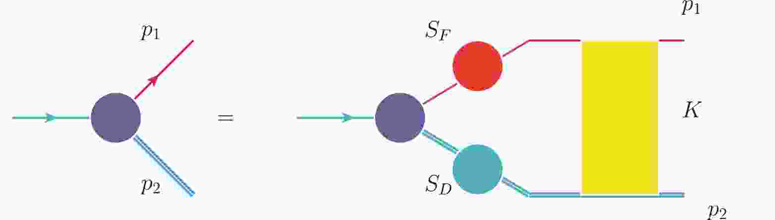
As shown in Fig. 1, following our previous research, the BS amplitude of
$ \Lambda_b(\Lambda) $ in momentum space satisfies the integral equation [28, 29, 33–39]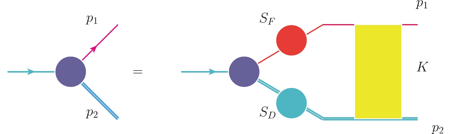
Figure 1. (color online) BS equation for
$ \Lambda_b(\Lambda) $ in momentum space (K is the interaction kernel)$ \chi_P(p) = S_{ \rm F}(\lambda_1 P+p)\int \frac{{\rm d}^4 q}{(2 \pi)^4} K (P,p,q)\chi_P(q)S_{ D}(\lambda_2 P-p), $

(3) where
$ K(P,p,q) $ is the kernel, which is defined as the sum of the two particles irreducible diagrams,$ S_{ \rm F} $ and$ S_{ D} $ are the propagators of the quark and scalar diquark, respectively.$ \lambda_{1(2)}=m_{q(D)}/(m_q+m_D) $ , where$ m_{q(D)} $ is the mass of the quark (diquark), and P is the momentum of the baryon.We assume the kernel has the following form:
$- {\rm i} K(P,p,q) = I\otimes I V_1(p,q)+ \gamma_\mu \otimes (p_2+q_2)^\mu V_2(p,q), $

(4) where
$ V_1 $ results from the scalar confinement, and$ V_2 $ is from the one-gluon-exchange diagram. According to the potential model,$ V_1 $ and$ V_2 $ have the following forms in the covariant instantaneous approximation ($ p_l=q_l $ ) [28, 29, 37–39]:$ \begin{aligned}[b] \tilde{V}_1(p_t-q_t) =& \frac{8 \pi \kappa}{[(p_t-q_t)^2+\mu^2]^2} - (2\pi)^2\delta^3(p_t-q_t)\\&\times\int \frac{{\rm d}^3k}{(2\pi)^3} \frac{8 \pi \kappa}{(k^2+\mu^2)^2}, \end{aligned} $

(5) $ \tilde{V_2} (p_t-q_t)=- \frac{16 \pi }{3}\frac{\alpha^2_{\rm seff} Q^2_0}{[(p_t-q_t)^2+\mu^2][(p_t-q_t)^2+Q_0^2]}, $

(6) where μ is a small parameter; to avoid the divergence in numerical calculation, this parameter is considered to be sufficiently small such that the results are not sensitive to it. The parameters κ and
$ \alpha_{\rm seff} $ are related to scalar confinement and the one-gluon-exchange diagram, respectively.$ q_t $ is the transverse projection of the relative momentum along the momentum P, which is defined as$ p_l = \lambda_1 P -v\cdot p,\; p_t^\mu = p^\mu-(v\cdot p)p^\mu $ $ (v^\mu=P^\mu/M ),$ $ q_t^\mu = q^\mu -(v \cdot q) v^\mu $ , and$ q_l= \lambda_2 P -v \cdot q $ . The second term of$ \tilde{V}_1 $ is introduced to avoid infrared divergence at the point$ p_t=q_t $ , and μ is a small parameter to avoid the divergence in numerical calculations. Analyzing the electromagnetic FFs of the proton,$ Q_0^2=3.2 $ GeV$ ^2 $ was observed to provide consistent results with the experimental data [40].The propagators of the quark and diquark can be expressed as follows:
$ S_F(p_1) = {\rm i} \not {v} \bigg[ \frac{\Lambda_q^+ }{ M -p_l -\omega_q +{\rm i} \epsilon} +\frac{\Lambda_q ^-}{ M -p_l +\omega_q -{\rm i} \epsilon}\bigg], $

(7) $ S_D(p_2) = \frac{\rm i}{2 \omega_D} \bigg[\frac{1}{ p_l-\omega_D+{\rm i} \epsilon} -\frac{1}{ p_l+ \omega_D-{\rm i}\epsilon}\bigg], $

(8) where
$ \omega_q = \sqrt{m^2-p_t^2}\; {\rm{and}}\; \omega_D = \sqrt{m_D^2-p_t^2} $ , M is the mass of the baryon, and$ \Lambda^\pm $ are the projection operators, which are defined as$ 2 \omega_q \Lambda^\pm_q= \omega_q \pm \not {v}(\not {p}_t+m) , $

(9) and satisfy the following relations:
$ \Lambda_q^\pm \Lambda_q^\pm = \Lambda^\pm_q,\; \Lambda^\pm_q \Lambda^\mp_q = 0. $

(10) Generally, we require two scalar functions to describe the BS wave function of
$ \Lambda_b(\Lambda) $ [33–35],$ \chi_P(p) = (f_1(p_t^2)+\not {p}_t f_2(p_t^2))u(P), $

(11) where
$ f_i, (i=1,2) $ are the Lorentz-scalar functions of$ p_t^2 $ , and$ u(P) $ is the spinor of a baryon.Defining
$ \tilde{f}_{1(2)}=\int \dfrac{{\rm d} p_l}{2 \pi}f_{1(2)} $ , and using the covariant instantaneous approximation, the scalar BS wave functions satisfy the following coupled integral equations:$ \tilde{f}_1(p_t) =\int \frac{{\rm d}^3q_t}{(2\pi)^3} M_{11}(p_t,q_t) \tilde{f}_1(q_t)+ M_{12}(p_t,q_t) \tilde{f}_2(q_t), $

(12) $ \tilde{f}_2(p_t) = \int \frac{{\rm d}^3q_t}{(2\pi)^3} M_{21}(p_t,q_t) \tilde{f}_1(q_t) + M_{22}(p_t,q_t) \tilde{f}_2(q_t), $

(13) where
$ \begin{aligned}[b] M_{11}(p_t,q_t)=&\frac{(\omega_q +m ) (\tilde{V}_1+ 2 \omega_D \tilde{V}_2)- p _t \cdot ( p _t+ q _t) \tilde{V}_2}{4 \omega_D \omega_q(-M + \omega_D+ \omega_q)} \\&- \frac{(\omega_q -m )(\tilde{V}_1- 2\omega_D \tilde{V}_2)+ p _t\cdot( p _t+ q _t) \tilde{V}_2}{4 \omega_D \omega_c(M + \omega_D+ \omega_q)}, \end{aligned} $

(14) $ \begin{aligned}[b] M_{12}(p_t,q_t)=&\frac{- (\omega_q+m ) ( q _t + p _t)\cdot q_t\tilde{V}_2 + p _t\cdot q_t(\tilde{V}_1- 2 \omega_D \tilde{V}_2)}{4 \omega_D \omega_c(-M + \omega_D+ \omega_c)}\\&- \frac{(m - \omega_q ) ( q _t + p _t)\cdot q _t \tilde{V}_2 - p _t\cdot q _t (\tilde{V}_1+ 2\omega_D \tilde{V}_2)}{4 \omega_D \omega_q(M + \omega_D+ \omega_q)}, \end{aligned} $

(15) $ \begin{aligned}[b] M_{21}(p_t,q_t)=& \frac{(\tilde{V}_1+ 2 \omega_D \tilde{V}_2)-( -\omega_q+m ) \left(1+\dfrac{ q _t \cdot p _t }{ p^2_t }\right)\tilde{V}_2}{4 \omega_D \omega_q(-M + \omega_D+ \omega_q)} \\& - \frac{- (\tilde{V}_1- 2\omega_D \tilde{V}_2)+(\omega_q + m )\left(1+\dfrac{ q _t \cdot p _t }{ p^2_t }\right) \tilde{V}_2}{4 \omega_D \omega_q(M + \omega_D+ \omega_q)}, \end{aligned} $

(16) $ \begin{aligned}[b]& M_{22}(p_t,q_t)\\=& \frac{(m -\omega_q)( \tilde{V}_1+ 2 \omega_D \tilde{V}_2)) p_t \cdot q_t - p^2_t ( q^2_t+ p_t \cdot q_t) \tilde{V}_2}{4 p^2_t \omega_D \omega_q(-M + \omega_D+ \omega_q)}\\&- \frac{ (m +\omega_q) (-\tilde{V}_1- 2 \omega_D \tilde{V}_2)) p_t \cdot q_t + p^2_t ( q^2_t+ p_t \cdot q_t)\tilde{V}_2 }{4 p^2_t \omega_D \omega_q(M + \omega_D+ \omega_q)}. \end{aligned} $

(17) When the mass of the b quark approaches infinity [32], the propagator of the b quark satisfies the relation
$ \not{ v} S_{ \rm F}(p_1)= S_{ \rm F}(p_1) $ and can be reduced to$ S_{ \rm F}(p_1) = {\rm i} \frac{ 1+ \not {v} }{ 2 (E_0+m_D -p_l+ {\rm i} \epsilon) }, $

(18) where
$ E_0=M-m-m_D $ is the binding energy. Thus, the BS wave function of$ \Lambda_b $ has the form$ \chi_P (v) = \phi (p)u_{\Lambda_b}(v,s) $ , where$ \phi(p) $ is the scalar BS wave function [32], and the BS equation for$ \Lambda_b $ can be replaced by$ \begin{aligned}[b] \phi(p) =& -\frac{\rm i}{(E_0+m_D-p_l+{\rm i} \epsilon)( p_l ^2-\omega^2_D)}\\&\times\int \frac{{\rm d}^4 q }{(2\pi)^4}(\tilde{V}_1+2 p_l \tilde{V}_2)\phi(q). \end{aligned} $

(19) Generally, we can take
$ E_0 $ to be about$ -0.14 $ GeV and κ to be about$ 0.05 $ GeV$ ^3 $ [28, 29]. -
In the Standard Model, the
$ \Lambda_b\rightarrow \Lambda l^+l^- $ ($ l=e,\mu, \tau $ ) transitions are described by$ b\rightarrow s l^+l^- $ at the quark level. The Hamiltonian for the decay of$ b\rightarrow s l^+l^- $ is given by$ \begin{aligned}[b] \mathcal{H}( b\rightarrow s l^+l^-) =& \frac{G_{\rm F}\alpha}{2 \sqrt{2}\pi}V_{\rm tb}V^*_{\rm ts}\bigg[ C^{\rm eff}_9 \bar{s} \gamma_{\mu}(1-\gamma_5)b \bar{l}\gamma^{\mu}l\\& - {\rm i} C^{\rm eff}_{7}\bar{s}\frac{2 m_b\sigma_{\mu\nu} q^{\nu}}{q^2}(1+\gamma_5) b \bar{l}\gamma^{\mu}l \end{aligned} $

$ \begin{aligned}[b]\quad +C_{10} \bar{s}\gamma_{\mu}(1-\gamma_5) b \bar{l}\gamma^{\mu}\gamma_5l \bigg], \end{aligned} $

(20) where
$ G_{\rm F} $ is the Fermi coupling constant, α is the fine structure constant at the Z mass scale,$ V_{\rm ts} $ and$ V_{\rm tb} $ are the CKM matrix elements, q is the total momentum of the lepton pair, and$ C_i\; (i=7,\; 9,\; 10) $ are the Wilson coefficients.$ C^{\rm eff}_7=-0.313 $ ,$ C^{\rm eff}_9=4.334 $ ,$ C_{10}=-4.669 $ [41–43]. The relevant matrix elements can be parameterized in terms of the FFs as follows:$ \begin{aligned}[b] \langle \Lambda(P^\prime) | \bar{s}\gamma_{\mu}b | \Lambda_b(P)\rangle =& \bar{u}_{\Lambda}(P^\prime)(g_1\gamma^\mu+ {\rm i}g_2\sigma^{\mu\nu}q_{\nu}+g_3q_\mu)u_{\Lambda_b}(P),\\ \langle \Lambda(P^\prime) | \bar{s}\gamma_{\mu}\gamma_{5}b | \Lambda_b(P)\rangle = & \bar{u}_{\Lambda}(P^\prime)(t_1\gamma^\mu+{\rm i}t_2\sigma^{\mu\nu}q_{\nu}+t_3q^\mu)\gamma_5u_{\Lambda_b}(P),\\ \langle \Lambda (P^\prime) | \bar{s}i\sigma^{\mu\nu}q^{\nu}b | \Lambda_b(P)\rangle = & \bar{u}_{\Lambda}(P^\prime)(s_1\gamma^\mu+{\rm i}s_2\sigma^{\mu\nu}q_{\nu}+s_3q^\mu)u_{\Lambda_b}(P),\\ \langle \Lambda (P^\prime) | \bar{s}i\sigma^{\mu\nu}\gamma_5q^{\nu}b | \Lambda_b(P)\rangle = & \bar{u}_{\Lambda}(P^\prime)(d_1\gamma^\mu+{\rm i}d_2\sigma^{\mu\nu}q_{\nu}+d_3q^\mu)\gamma_5u_{\Lambda_b}(P), \end{aligned} $ 
(21) where
$ P (P^\prime) $ is the momentum of the$ \Lambda_b $ (Λ),$ q^2= (P-P^\prime)^2 $ is the transformed momentum squared, and$ g_i $ ,$ t_i $ ,$ s_i $ , and$ d_i $ ($ i=1,2 $ , and 3) are the transition FFs, which are Lorentz scalar functions of$ q^2 $ . The$ \Lambda_b $ and Λ states can be normalized as follows:$ \langle \Lambda(P^\prime)|\Lambda(P)\rangle = 2 E_\Lambda (2\pi)^3 \delta^3(P-P^\prime), $

(22) $ \langle \Lambda_b(v^\prime,P^\prime)|\Lambda_b(v,P)\rangle = 2 v_0(2\pi)^3 \delta^3(P-P^\prime). $

(23) Comparing Eq. (1) with Eq. (21), we obtain the following relations:
$ \begin{aligned}[b] & g_1\; =\; t_1\; =\; s_2\; =\; d_2\; =\; \bigg(F_1+\sqrt{r}F_2\bigg),\\ & g_2\; =\; t_2\; =g_3\; =\; t_3\; =\; \frac{1}{m_{\Lambda_{b}}}F_2, \\ & s_3\; =\; F_2 (\sqrt{r}-1),\quad d_3\; =\; F_2(\sqrt{r}+1), \\ & s_1 \; =\; d_1\; =\; F_2 m_{\Lambda_b} (1+r-2\sqrt{r}\omega), \end{aligned} $

(24) where
$ r=m_\Lambda^2/m_{\Lambda_b}^2 $ and$ \omega= (M_{\Lambda_b}^2+M_{\Lambda}^2-q^2)/ (2M_{\Lambda_b} M_{\Lambda})= v\cdot P^\prime/m_{\Lambda} $ . The transition matrix for$ \Lambda_b\rightarrow \Lambda $ can be expressed in terms of the BS wave functions of$ \Lambda_b $ and Λ:$ \langle \Lambda (P^\prime)|\bar{d}\Gamma b|\Lambda_b(P)\rangle =\int\frac{{\rm d}^4p}{(2\pi)^4} \bar{\chi}_{P^\prime}(v^\prime)\Gamma \chi_P(p)S^{-1}_{ D}(p_2). $

(25) When
$ \omega \neq 1 $ , we can obtain the following expression by substituting Eqs. (11) and (19) into Eq. (25):$ F_1 = k_1- \omega k_2, $

(26) $ F_2 = k_2, $

(27) where
$ k_1(\omega)=\int \frac{{\rm d}^4p}{(2 \pi)^4} f_1(p^\prime) \phi(p) S^{-1}_{ D}(p_2), $

(28) $ k_2(\omega) = \frac{1}{1-\omega^2} \int \frac{{\rm d}^4 p}{(2\pi)^4} f_2(p^\prime) p^\prime_t \cdot v \phi(p) S^{-1}_{ D}. $

(29) The decay amplitude of
$ \Lambda_b \rightarrow \Lambda l^+ l^- $ can be rewritten as follows:$ \begin{aligned}[b] \mathcal{M}(\Lambda_b\rightarrow \Lambda l^+ l^-)=&\frac{G_{\rm F} \lambda_t}{2\sqrt{2}\pi} \big[\bar{l}\gamma_{\mu}l\{\bar{u}_{\Lambda}[\gamma_{\mu}(A_1+B_1+ (A_1-B_1)\gamma_5 ) \\ & + {\rm i}\sigma^{\mu\nu}p_{\nu}(A_2+B_2+ (A_2-B_2)\gamma_5 )]u_{\Lambda_b}\} \\ &+\bar{l}\gamma_{\mu}\gamma_5l\{\bar{u}_{\Lambda}[\gamma^{\mu}(D_1+E_1+ (D_1-E_1)\gamma_5 ) \\ &+{\rm i}\sigma^{\mu\nu}p_{\nu}(D_2+E_2+ (D_2-E_2)\gamma_5 )\\ &+p^{\mu}(D_3+E_3+ (D_3-E_3)\gamma_5 )]u_{\Lambda_b}\}\big], \end{aligned} $

(30) where
$ A_i $ ,$ B_i $ ,$ D_j $ , and$ E_j $ ($ i=1,2 $ and$ j=1,2,3 $ ) are defined as follows:$ \begin{aligned}[b] &A_i=\frac{1}{2}\bigg\{C^{\rm eff}_{9}(g_i-t_i)-\frac{2C^{\rm eff}_7 m_b}{q^2}(d_i +s_i )\bigg\},\\ & B_i = \frac{1}{2}\bigg\{C^{\rm eff}_{9}(g_i+t_i) - \frac{2C^{\rm eff}_7m_b}{q^2}(d_i -s_i )\bigg\}, \\ & D_j = \frac{1}{2}C_{10}(g_j-t_j), \; E_j=\frac{1}{2}C_{10}(g_j+t_j). \end{aligned} $

(31) In the physical region (
$ \omega = (m_{\Lambda_b}^2 + m_{\Lambda}^2 -q^2)/ (2m_{\Lambda_b}m_{\Lambda}) $ ), the decay rate of$ \Lambda_b\rightarrow \Lambda l^+l^- $ is obtained as follows:$ \frac{{\rm d}\Gamma(\Lambda_b\rightarrow \Lambda l^+l^-)}{{\rm d}\omega {\rm d} \cos \theta}=\frac{G^2_{\rm F}\alpha^2}{2^{14}\pi^5m_{\Lambda_b}} |V_{\rm tb}V^*_{\rm ts}|^2v_l\sqrt{\lambda(1,r,s)} \mathcal{M}(\omega, \theta) , $

(32) where
$ s= 1 +r - 2 \sqrt{r} \omega $ ,$\lambda(1,r,s)=1+r^2+s^2-2r- 2s- 2rs$ ,$ v_l=\sqrt{1-\dfrac{4m^2_l}{s m^2_{\Lambda_b}}} $ , and the decay amplitude is expressed as follows [44]:$ \mathcal{M}(\omega,\theta) = \mathcal{M}_0(\omega) +\mathcal{M}_1(\omega) \cos \theta +\mathcal{M}_2(\omega) \cos^2 \theta, $

(33) where θ is the polar angle, as shown in Fig. 2.

Figure 2. (color online) Definition of the angle θ in the decay
$ \Lambda_b \rightarrow \Lambda l^- l^+ $ .$ \begin{aligned}[b] \mathcal{M}_0(\omega)=&32m^2_l m^4_{\Lambda_b}s(1+r-s)(|D_3|^2+|E_3|^2) +64m^2_lm^3_{\Lambda_b}(1-r-s){\rm Re}(D^*_1E_3+D_3E^*_1)\\ &+64m^2_{\Lambda_b}\sqrt{r}(6m^2_l-M^2_{\Lambda_b}s){\rm Re}(D_1^*E_1) + {64m^2_lm^3_{\Lambda_b}\sqrt{r}\big(2m_{\Lambda_b}s {\rm Re}(D^*_3E_3) +(1-r+s){\rm Re}(D^*_1D_3+E^*_1E_3)\big) }\\ &+32m^2_{\Lambda_b}(2m^2_l+m^2_{\Lambda_b}s)\bigg\{(1-r+s)m_{\Lambda_b}\sqrt{r}{\rm Re}(A^*_1A_2+B^*_1B_2)\\ &-m_{\Lambda_b}(1-r-s){\rm Re}(A^*_1B_2+A^*_2B_1) -2\sqrt{r}\big({\rm Re}(A^*_1B_1)+m^2_{\Lambda_b}s {\rm Re}(A^*_2B_2)\big) \bigg \}\\ & + 8 m^2_{\Lambda_b}\bigg[4m^2_l(1-r-s)+m^2_{\Lambda_b}((1+r)^2- s^2)\bigg](|A_1|^2+|B_1|^2)\\ &+8m^4_{\Lambda_b}\bigg\{4m^2_l[\lambda+(1+r-s)s]+m^2_{\Lambda_b}s[(1-r)^2-s^2]\bigg\}(|A_2|^2+|B_2|^2) \\ & - 8m^2_{\Lambda_b}\bigg\{4m^2_l(1+r-s)-m^2_{\Lambda_b}[(1-r)^2-s^2]\bigg\} (|D_1|^2+|E_1|^2) \\ &+ 8m^5_{\Lambda_b}sv^2\bigg\{-8m_{\Lambda_b}s\sqrt{r}{\rm Re}(D^*_2E_2) +4(1-r+s)\sqrt{r}{\rm Re}(D^*_1D_2+E^*_1E_2)\\ & -4(1-r-s) {\rm Re}(D^*_1E_2+D^*_2E_1)+m_{\Lambda_b}[(1-r)^2-s^2] (|D_2|^2+|E_2|^2)\bigg\}, \end{aligned} $ 
(34) $ \begin{aligned}[b] {\mathcal M}_1(\omega) =& -16 m_{\Lambda_b}^4 s v_l \sqrt{\lambda} \Big\{ 2 {\rm Re}(A_1^* D_1)-2{\rm Re}(B_1^* E_1)+ 2m_{\Lambda_b} {\rm Re}(B_1^* D_2-B_2^* D_1+A_2^* E_1-A_1^*E_2)\Big\}\\ &+32 m_{\Lambda_b}^5 s v_l \sqrt{\lambda} \Big\{ m_{\Lambda_b} (1-r){\rm Re}(A_2^* D_2 -B_2^* E_2)+ \sqrt{r} {\rm Re}(A_2^* D_1+A_1^* D_2-B_2^*E_1-B_1^* E_2)\Big\}, \end{aligned} $

(35) $ \mathcal{M}_2(\omega) = 8m^6_{\Lambda_b}s v_l^2\lambda(|A_2|^2+|B_2|^2+|E_2|^2+|D_2|^2) - 8 m^4_{\Lambda_b}v_l^2\lambda(|A_1|^2+|B_1|^2+|E_1|^2+|D_1|^2). $

(36) The lepton-side forward-backward asymmetry,
$ A_{\rm FB} $ , is defined as$ A_{\rm FB} = \frac{\displaystyle\int_{0}^{1} \dfrac{{\rm d} \Gamma}{{\rm d} q^2 {\rm d}z} {\rm d}z -\displaystyle\int_{-1}^{0} \dfrac{{\rm d} \Gamma}{{\rm d} q^2 {\rm d}z} {\rm d}z }{\displaystyle\int_{-1}^{1} \dfrac{{\rm d} \Gamma}{{\rm d} q^2 {\rm d}z} {\rm d}z }, $

(37) where
$ z = \cos \theta $ . The "naively integrated" observables are obtained using [17]$ \langle {X}\rangle = \frac{1}{q^2_{\rm max}- q^2_{\rm min}} \int_{q^2_{\rm min}}^{q^2_{\rm max}}X(q^2){\rm d} q^2. $

(38) We define the integrated
$ A_{\rm FB} $ as$ \bar{A}_{\rm FB} = \int_{\hat{q}_{\rm min}}^{\hat{q}_{\rm max}} {\rm d} \hat{q}^2 A_{\rm FB}(\hat{q}^2). $

(39) where
$ \hat{q}^2= q^2 / M_{\Lambda_b}^2 $ . With the aid of the helicity amplitudes of$ \Lambda_b \rightarrow \Lambda l^+ l^- $ , we can also calculate the hadron forward-backward asymmetry, the lepton-hadron side asymmetry, and the fraction of longitudinally polarized dileptons.The hadron forward-backward asymmetry has the form
$ \begin{aligned}[b]& A_{\rm FB}^h(q^2) \\=&\frac{\alpha_\Lambda}{2} \frac{ \dfrac{v^2_l}{2} ({\cal H}_P^{11}+{\cal H}_P^{22}+{\cal H}_{L_P}^{11}+{\cal H}_{L_P}^{22})+\dfrac{3m_l^2}{q^2}({\cal H}_{P}^{11}+{\cal H}_{L_P}^{11}+{\cal H}_{S_P}^{22})}{{\cal H}_{\rm tot}}.\qquad \end{aligned} $

(40) The lepton-hadron side asymmetry has the form
$ \begin{equation} A_{\rm FB}^{lh}(q^2) =-\frac{3}{4} \frac{\alpha_\Lambda}{2} \frac{v_l {\cal H}_U^{12} } {{\cal H}_{\rm tot}}.\qquad \end{equation} $

(41) The fraction of the longitudinally polarized dileptons is expressed by
$ \begin{equation} F_L(q^2)=\frac{\dfrac{v^2_l}{2}({\cal H}_L^{11}+{\cal H}_{L}^{22})+ \dfrac{m_l^2}{q^2}({\cal H}_{U}^{11}+{\cal H}_{L}^{11}+{\cal H}_{S}^{22})}{{\cal H}_{\rm tot}}. \end{equation} $

(42) In Eqs. (40–42),
$ {\cal H}_{X}^{m m^\prime} (X= U,\; L,\; S,\; P,\; L_P,\; S_P,\; m=1,2) $ represent different helicity amplitudes, and$ {\cal H}_{\rm tot} $ is the total helicity amplitude,$ \alpha_\Lambda=0.642\pm0.013 $ . The explicit expression for$ {\cal H}^{mm^\prime}_{X} $ is provided in Ref. [12]. -
In this section, we perform a detailed numerical analysis of
$ A_{\rm FB}(\Lambda_b \rightarrow \Lambda l^+ l^-) $ . In this study, we take the masses of baryons as$ m_{\Lambda_b}=5.62 $ GeV and$ m_\Lambda=1.116 $ GeV [45], and the masses of quarks as$ m_b=5.02 $ GeV and$ m_s=0.516 $ GeV [34, 35, 39]. The variable ω changes from$ 1 $ to$ 2.617,\; 2.614,\; 1.617 $ for$ e,\; \mu,\; \tau $ , respectively.Solving Eqs. (12) and (19) for Λ and
$ \Lambda_b $ , we can obtain the numerical solutions of their BS wave functions. In Table 1, we provide the values of$ \alpha_{\rm seff} $ for different values of κ for Λ and$ \Lambda_b $ with$ E_0=-0.14 $ GeV.κ/GeV $ ^3 $ 

Λ $ \Lambda_b $ 

0.045 0.559 0.775 0.047 0.555 0.777 0.049 0.551 0.778 0.051 0.547 0.780 0.053 0.544 0.782 0.055 0.540 0.784 Table 1. Values of
$\alpha_{\rm seff}$ for Λ and$ \Lambda_b $ for different κ values.From Table 1, we observe that the value of
$ \alpha_{\rm seff} $ is weakly dependent on the value of κ. In Fig. 3, we plot the FFs and FF ratio$ R(\omega) $ . From this figure, we observe that$ R(\omega) $ varies from$ -0.75 $ to$ -0.25 $ in our model. In Ref. [27],$ R(\omega) $ varied from$ -0.42 $ to$ -0.83 $ in the same ω region, which is in agreement with our result and the estimated value from Refs. [28, 29] mentioned in the Introduction. In the range of$ 2.43 \leq \omega \leq 2.52 $ (corresponding to$ M_\Lambda^2 \leq q^2 \leq M_{\Lambda_c}^2 $ ),$ R(\omega) $ is about$ -0.25 $ . In the same ω region, assuming the FFs have the same dependence on$ q^2 $ , the CLEO collaboration measured$ R=-0.35\pm 0.04\pm0.04 $ in the limit$ m_c \rightarrow + \infty $ . These results are in good agreement with our research in the same ω region.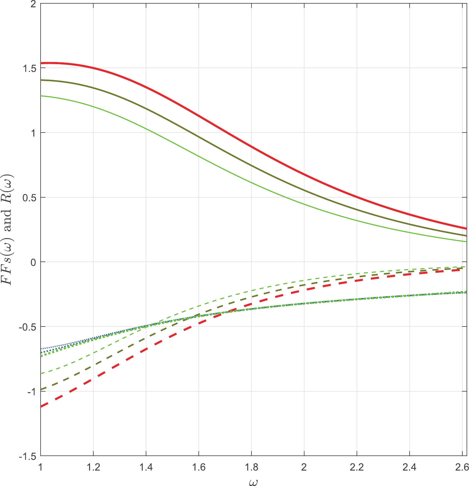
Figure 3. (color online) Values of
$ F_1 $ (solid line),$ F_2 $ (dash line) and$ R(\omega) $ (dot line) as a function of ω (the lines become thicker with the increase in κ).In Table 2, we provide
$ \bar{A}^l_{\rm BF} $ ,$ \bar{A}^{lh}_{\rm FB} $ ,$ \bar{A}^h_{\rm FB} $ , and$ \bar{F}_L $ for$ \Lambda_b \rightarrow \Lambda \mu^+ \mu^- $ and compare our results with those of other studies. We can observe that these asymmetries differ significantly in different models. Considering these differences,$ \bar{A}^l_{\rm FB} $ changes between$ -0.30 $ and$ 0 $ ,$ \bar{A}^{lh}_{\rm FB} $ is about$ 0.1 $ ,$ \bar{A}^h_{\rm FB} $ is about$ -0.25 $ , and$ \bar{F}_L $ changes from$ 0.3 $ to$ 0.6 $ . Without including the long distance contribution, Ref. [6] provided the integrated forward-backward asymmetry$ \bar{A}^l_{\rm BF}(\Lambda_b \rightarrow \Lambda \mu^+ \mu^-)= -0.1338 $ . The result of Ref. [7] was$ \bar{A}^l_{\rm BF}(\Lambda_b \rightarrow \Lambda \mu^+ \mu^-)= -0.13(-0.12) $ in the QCD sum rule approach (pole model). Using the covariant constituent quark model with (without) the long distance contribution, Ref. [8] obtained the result$ \bar{A}^l_{\rm BF}(\Lambda_b \rightarrow \Lambda \mu^+ \mu^-)= 1.7\times 10^{-4} (8\times 10^{-4}) $ .$ \bar{A}^l_{\rm FB} $ 

$ \bar{A}^{lh}_{\rm FB} $ 

$ \bar{A}^{h}_{\rm FB} $ 

$ \bar{F}_L $ 

[6, 7] $ -0.13 $ 

− − $ 0.5830 $ 

[8] $ 8.0\times 10^{-4} $ 

− − − [12] $ -0.286 $ 

$ 0.101 $ 

$ -0.288 $ 

$ 0.525 $ 

[13] $ -0.0122^{+0.0142}_{-0.0073} $ 

− − − [15] $ -0.29\pm0.05 $ 

$ 0.13^{+0.22}_{-0.03} $ 

$ -0.26\pm0.03 $ 

$ 0.4\pm0.1 $ 

[17] $ -0.04^{+0.00}_{-0.01} $ 

− − $ 0.34_{-0.02}^{+0.03} $ 

our work $ -0.1376\pm0.0001 $ 

$ 0.0576 $ 

$ - 0.1613\pm0.0001 $ 

$ 0.3957\pm0.0002 $ 

Table 2. Longitudinal polarization fractions and forward-backward asymmetries for
$ \Lambda_b \rightarrow \Lambda \mu^+ \mu^- $ .For
$ q^2 \in [15,20] $ GeV$ ^2 $ , the LHCb collaboration provided$ {A}^l_{\rm FB}(\Lambda_b \rightarrow \Lambda \mu^- \mu^+) = -0.05 \pm 0.09 $ in 2015, which was updated to$ {A}^l_{\rm FB}(\Lambda_b \rightarrow \Lambda \mu^- \mu^+) = -0.39 \pm 0.04 $ three years later [4, 5]. In our study, in the same region, the value of$ {A}^l_{\rm BF}(\Lambda_b \rightarrow \Lambda \mu^- \mu^+) $ changes from$ -0.44 $ to$ -0.35 $ , which is in good agreement with the most recent experimental data of the LHCb collaboration. With the latest high-precision lattice QCD calculations in the same region, Ref. [46] obtained the values$ {A}^l_{\rm FB}(\Lambda_b \rightarrow \Lambda \mu^- \mu^+) = -0.344 $ in the large$ \varsigma_u $ and small$ \varsigma_d $ regions ($ \varsigma_u,\; \varsigma_d $ are model parameters [47]) and$ {A}^l_{\rm FB}(\Lambda_b \rightarrow \Lambda \mu^- \mu^+) =-0.24 $ in the large$ \varsigma_d $ and small$ \varsigma_u $ regions. In Fig. 4, we plot the$ q^2 $ -dependence of$ A^l_{\rm FB}(\Lambda_b \rightarrow \Lambda e^- e^+) $ ,$ A^l_{\rm FB}(\Lambda_b \rightarrow \Lambda \mu^- \mu^+) $ , and$ A^l_{\rm FB}(\Lambda_b \rightarrow \Lambda \tau^- \tau^+) $ . From Fig. 4, we can observe that$ A^l_{\rm FB}(\Lambda_b\rightarrow \Lambda \mu^+ \mu^-) $ is in good agreement with the lattice QCD calculation in the entire$ q^2 $ region [48]. The results of other references results are also shown in Table 3. In Fig. 5, we plot the$ q^2 $ -dependence of$ A^h_{\rm FB}(\Lambda_b \rightarrow \Lambda e^- e^+) $ ,$ A^h_{\rm FB}(\Lambda_b \rightarrow \Lambda \mu^- \mu^+) $ , and$ A^h_{\rm FB}(\Lambda_b \rightarrow \Lambda \tau^- \tau^+) $ , respectively. For$ q^2 \in [15,20] $ GeV$ ^2 $ , the LHCb collaboration obtained the value for$ \Lambda_b \rightarrow \Lambda \mu^- \mu^+ $ as$ -0.29\pm0.07 $ , which is in good agreement our result$ -0.2304\sim -0.0685 $ . The results of other references results are also shown in Table 3. In Fig. 6, we plot the$ q^2 $ -dependence of$ A^{lh}_{\rm FB}(\Lambda_b \rightarrow \Lambda e^- e^+) $ ,$ A^{lh}_{\rm FB}(\Lambda_b \rightarrow \Lambda \mu^- \mu^+) $ , and$ A^{lh}_{\rm FB}(\Lambda_b \rightarrow \Lambda \tau^- \tau^+) $ , respectively. Ref. [12] obtained the value$ A^{lh}_{\rm FB}(\Lambda_b \rightarrow \Lambda \mu^- \mu^+) = 0.145 $ , which is agreement with our results$ 0.1257\sim0.1555 $ in the region$ q^2 \in [15,20] $ GeV$ ^2 $ . In Fig. 7, we plot the$ q^2 $ -dependence of$ F_L(\Lambda_b \rightarrow \Lambda e^- e^+) $ ,$ F_L(\Lambda_b \rightarrow \Lambda \mu^- \mu^+) $ , and$ F_L(\Lambda_b \rightarrow \Lambda \tau^- \tau^+) $ , respectively. In the region$ q^2 \in [15,20] $ GeV$ ^2 $ , the LHCb collaboration obtained the value$ F_L(\Lambda_b \rightarrow \Lambda \mu^- \mu^+)=0.61_{-0.14}^{+0.11} $ , which is close to our result of$ 0.3398\sim0.4530 $ . The results of other references results are also shown in Table 3. From these figures, we observe that all these asymmetries are not very sensitive to the parameters κ and$ E_0 $ in our model.− $ A^l_{\rm FB [15,20]} $ 

$ {A}^{lh}_{\rm FB[15,20]} $ 

$ {A}^{h}_{\rm FB[15,20]} $ 

$ {F}_{L[15,20]} $ 

LHCb [4, 5] $ -0.39\pm0.04 $ 

− $ -0.29\pm0.07 $ 

$ 0.61^{+0.11}_{-0.14} $ 

[6, 7] $ -0.40\sim-0.25 $ 

− − $ 0.37\sim 0.62 $ 

[8] $ -0.24\sim -0.13 $ 

− $>-0.308 $ 

− [12] $ -0.40 $ 

$ 0.145 $ 

$ -0.29 $ 

$ 0.38 $ 

[13] $ -0.075\sim -0.017 $ 

− − − [17] $ -0.34_{-0.02}^{+0.01} $ 

− − $ 0.4^{+0.01}_{-0.02} $ 

[48] $ -0.350(13) $ 

− $ -0.2710\pm0.0092 $ 

$ 0.409\pm0.013 $ 

our work $ -0.44\sim-0.35 $ 

$ 0.1257\sim 0.1555 $ 

$ -0.2304\sim-0.0685 $ 

$ 0.3398\sim0.4530 $ 

Table 3. Longitudinal polarization fractions and forward-backward asymmetries for
$ \Lambda_b \rightarrow \Lambda \mu^+ \mu^- $ in$ q^2 \in [15,20] $ GeV$ ^2 $ .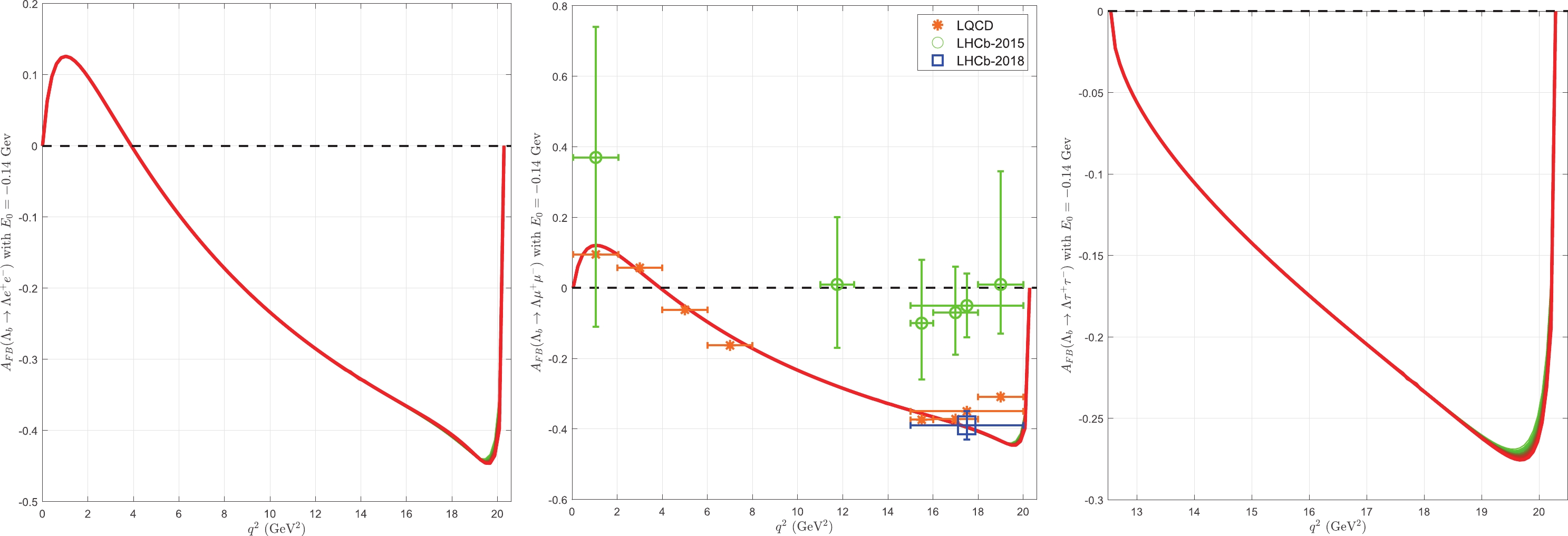
Figure 4. (color online) Values of
$A_{\rm FB}(\Lambda_b\rightarrow \Lambda l^+ l^-)$ as a function of$q^2$ for different values of κ as shown in Table 1.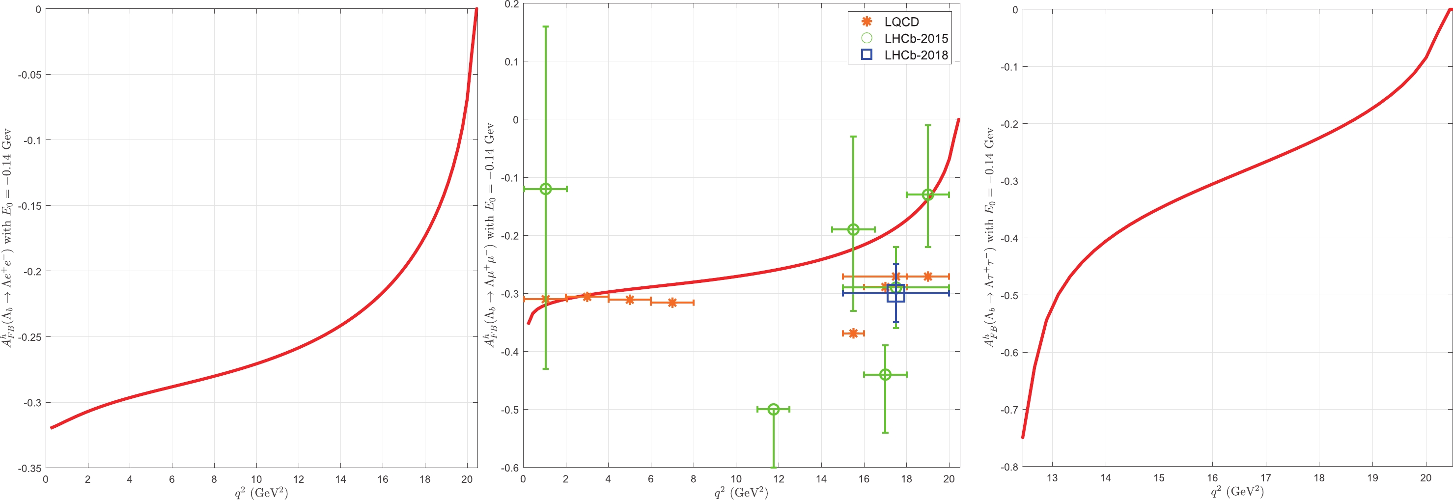
Figure 5. (color online) Values of
$A^h_{\rm FB}(\Lambda_b\rightarrow \Lambda l^+ l^-)$ as a function of$q^2$ for different values of κ as shown in Table 1.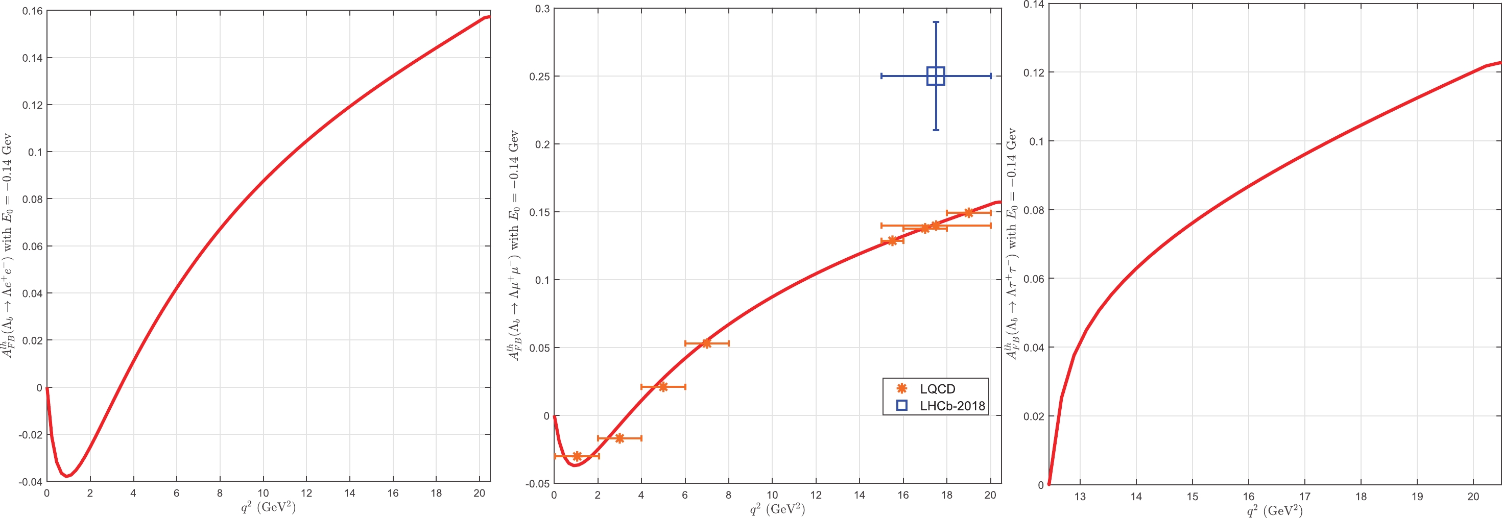
Figure 6. (color online) Values of
$A^h_{\rm FB}(\Lambda_b\rightarrow \Lambda l^+ l^-)$ as a function of$q^2$ for different values of κ as shown in Table 1.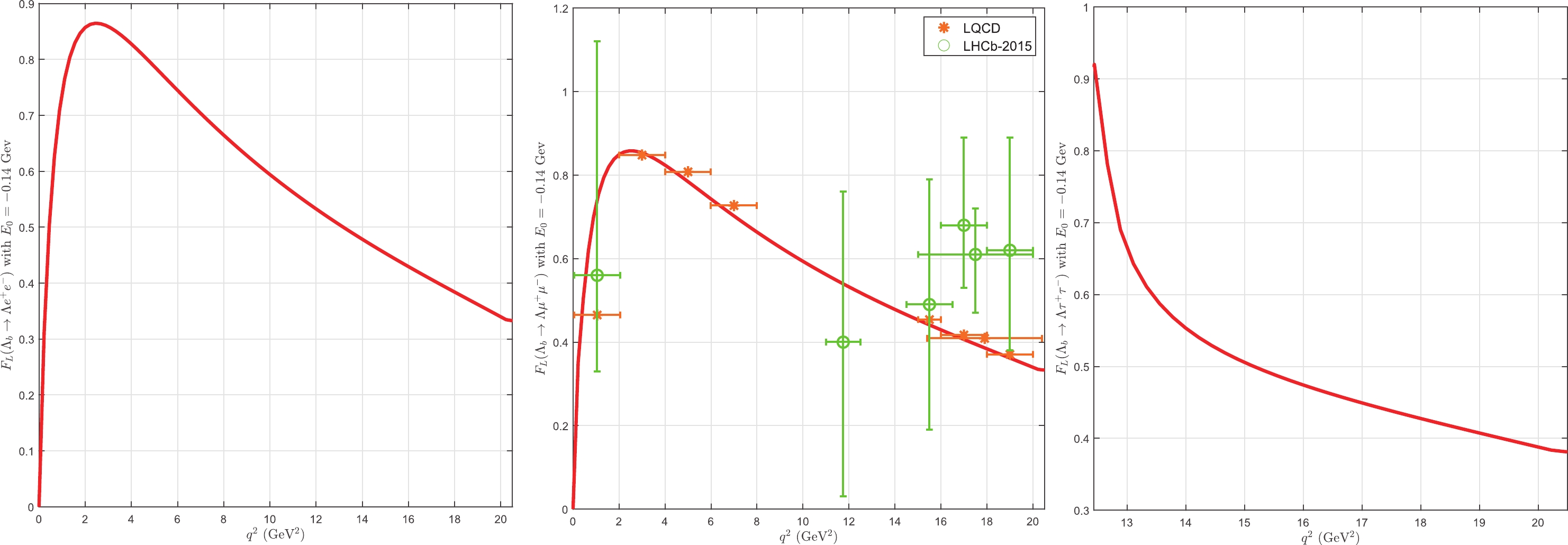
Figure 7. (color online) Values of
$F_L(\Lambda_b\rightarrow \Lambda l^+ l^-)$ as a function of$q^2$ for different values of κ as shown in Table 1.Ref. [17] obtained the naively integrated values
$ \langle A_{\rm FB}^l \rangle = -0.19^{+0.00}_{-0.01} $ and$ \langle F_L \rangle = 0.6\pm0.02 $ for$ \Lambda_b \rightarrow \Lambda \mu^+ \mu^- $ , whereas in our paper, these values are$ -0.1976 $ and$ 0.5681 $ , respectively. Our results are very close to those of Ref. [17]. In our paper, we obtain$ \bar{A}^l_{\rm FB}= -0.0708\pm 0.0001(-0.0590\pm0.0001) $ and$ \bar{A}^{h}_{\rm FB}=-0.1604\pm 0.0001 (-0.1541\pm0.0002) $ for$ \Lambda_b\rightarrow \Lambda e^+ e^-(\Lambda_b\rightarrow \Lambda \tau^+ \tau^-) $ . The values given in Ref. [8] are$ \bar{A}^l_{\rm FB}=1.2\times 10^{-8}(9.6\times 10^{-4}) $ and$ \bar{A}^{h}_{\rm FB}=-0.321(-0.259) $ , and Refs. [13] and [7] provide$ \bar{A}^l_{\rm FB}=-0.0067 $ and$ \bar{A}^l_{\rm FB}=-0.04 $ for$ \Lambda_b\rightarrow \Lambda \tau^+ \tau^- $ . Comparing the values in these theoretical approaches, we observe that the asymmetries may vary widely among the theoretical models because the FFs in these models are different. -
In this study, we use the BSE to study the forward-backward asymmetries in the rare decays
$ \Lambda_b \rightarrow \Lambda l^+ l^- $ in a covariant quark-diquark model. In this picture,$ \Lambda_b (\Lambda) $ is considered a bound state of a$ b(s) $ -quark and a scalar diquark.We establish the BSE for the quark and scalar diquark system and then derive the FFs of
$ \Lambda_b \rightarrow \Lambda $ . We solve the BS equation of this system and then provide the values of the FFs and R. We observe that the ratio R is not a constant, which is in agreement with Ref. [26] and the pQCD scaling law [23–25]. Using these FFs, we calculate the forward-backward asymmetries$ A^l_{\rm FB} $ ,$ A^{lh}_{\rm FB} $ , and$ A^h_{\rm FB} $ and longitudinal polarization fractions$ F_L $ and the integrated forward-backward asymmetries$ \bar{A}^l_{\rm FB} $ ,$ \bar{A}^{lh}_{\rm FB} $ , and$\bar{A}^h_{\rm FB}$ as well as$ \bar{F}_L $ for$ \Lambda_b \rightarrow \Lambda l^+l^- (l=e,\; \mu,\; \tau) $ . Comparing with other theoretical studies, we observe that the FFs are different; thus, these asymmetries are different. The long distance contributions are not included in this paper. They will be considered in our future research to compare the experimental data more exactly.
Forward-backward asymmetries in ${\boldsymbol \Lambda_{\boldsymbol b} \boldsymbol\rightarrow \boldsymbol\Lambda l^+ l^- }$ in the Bethe-Salpeter equation approach
- Received Date: 2022-03-08
- Available Online: 2022-09-15
Abstract: Using the Bethe-Salpeter equation (BSE), we investigate the forward-backward asymmetries


 DownLoad: