


 Abstract
 HTML
HTML Reference
 Related
 PDF
PDF


-
The systematic study of one-loop Feynman integrals in perturbative quantum field theories dates back to the end of the 1970s when 't Hooft and Veltman [1] calculated generic one-, two-, three-, and four-point scalar integrals in dimensional regularization (DREG) up to order
$ \epsilon^0 $ , where$ \epsilon=(4-d)/2 $ with spacetime dimension d. Passarino and Veltman [2] then demonstrated that tensor integrals up to four points can be systematically reduced to scalar ones, and later studies [3, 4] demonstrated that integrals with more than four external legs in$ 4-2\epsilon $ dimensions can be expressed as lower-point ones up to order$ \epsilon^0 $ . These developments in principle solved the problem of next-to-leading order (NLO) calculations for tree-induced scattering processes.The improvements of experimental precision and the progress of theoretical studies require the understanding of scattering amplitudes and cross sections at higher orders in perturbation theory. Hence, we must compute the one-loop integrals to higher orders in
$ \epsilon $ . These enable us to predict the infrared divergences appearing in two-loop amplitudes [5–13], and they are necessary for computing one-loop squared amplitudes, which are essential ingredients of next-to-next-to-leading order (NNLO) cross sections.Unlike the terms up to order
$ \epsilon^0 $ , generic results for the higher order terms are not available yet. Part of the reason is that integrals with more than four external legs are generally not reducible to lower-point ones when considering higher orders in ϵ. These require further calculations, which are often complicated owing to the increasing number of physical scales involved.It is known [14–16] that one-loop integrals in a given family admit a uniform transcendentality (UT) basis satisfying canonical differential equations of the form [17]
$ d \vec{f}(\vec{x},\epsilon) = \epsilon \, d{\boldsymbol{A}}(\vec{x}) \, \vec{f}(\vec{x},\epsilon) \, , $

(1) where
$ \vec{x} $ is the set of independent kinematic variables, and the matrix$ d{\boldsymbol{A}} $ has the$ d\log $ -form:$ d{\boldsymbol{A}}(\vec{x}) = \sum\limits_i {\boldsymbol{C}}_i \, d\log(W_i(\vec{x})) \, . $

(2) In the above expression,
$ {\boldsymbol{C}}_i $ are matrices consisting of rational numbers, and$ W_i(\vec{x}) $ are algebraic functions of the variables. The functions$ W_i $ are called the "letters" for this integral family, and the set of all independent letters is called the "alphabet."At one loop, a canonical basis can be generically constructed by searching for
$ d\log $ -form integrands [14–23]. However, obtaining the$ d\log $ matrix$ d{\boldsymbol{A}}(\vec{x}) $ is not always a trivial task when the number of variables is large. We note that the$ d\log $ matrix can be easily reconstructed if we have the knowledge of the alphabet$ \{W_i(\vec{x})\} $ in advance, since the coefficient matrices$ {\boldsymbol{C}}_i $ can then be obtained by bootstrapping.Having the alphabet (and hence the matrix
$ d{\boldsymbol{A}}(\vec{x}) $ ) in a good form also aids in solving the differential equations (1) order-by-order in the dimensional regulator$ \epsilon $ . The (suitably normalized) solution can be expressed as a Taylor series:$ \vec{f}(\vec{x},\epsilon) = \sum\limits_{n=0}^{\infty} \epsilon^n \, \vec{f}^{\,(n)}(\vec{x}\,) \, , $

(3) where the nth-order coefficient function can be expressed as a Chen iterated integral [24]:
$ \vec{f}^{(n)}(\vec{x}) =\int_{\vec{x}_0}^{\vec{x}} d{\boldsymbol{A}}(\vec{x}_n) \cdots \int_{\vec{x}_0}^{\vec{x}_2} d{\boldsymbol{A}}(\vec{x}_1) + \vec{f}^{(n)}(\vec{x}_0) \, . $

(4) Such iterated integrals can be analyzed using the language of "symbols" [25–27] that encodes the algebraic properties of the resulting functions. In certain scenarios, these iterated integrals can be solved analytically (either by direct integration or by bootstrapping). The results can often be expressed in terms of generalized polylogarithms (GPLs) [28], which enable efficient numeric evaluation [29–31]. When an analytic solution is not available, they can straightforwardly evaluated numerically through either numerical integration or series expansion [32, 33].
In this paper, we describe a generic method to construct the letters systematically from cut integrals in the Baikov representation [34, 35]. The letters can be generically expressed in terms of various Gram determinants. The letters and symbols of one-loop integrals were considered in [36–39], and our method is similar to that in [37–39]. Nevertheless, we evaluate the cut integrals differently and obtain equivalent but simpler expressions in certain cases utilizing the properties of Gram determinants. Furthermore, we consider the cases of divergent cut integrals, which were ignored in earlier studies. Using our results, all letters for a given integral family can be easily expressed even before constructing the differential equations. These letters will also appear in the corresponding two-loop integrals.
-
We use the method of [16, 23] to construct the canonical basis in the Baikov representation. In this section, we briefly review the construction procedure since it will also be relevant for obtaining the alphabet in the matrices
$ d{\boldsymbol{A}}(\vec{x}) $ .Consider a generic one-loop integral topology with
$ N = E + 1 $ external legs, where E is the number of independent external momenta. Integrals in this topology can be expressed as$ I_{a_1, \cdots, a_N} = \int \frac{{\rm d}^dl}{{\rm i} \pi^{d/2}} \frac{1}{z_1^{a_1} z_2^{a_2}\cdots z_N^{a_N}} \,, $

(5) where
$ z_i $ are the propagator denominators given by$ \begin{aligned}[b]& z_1=l^2-m_1^2 \,, \quad z_2= (l+p_1)^2-m_2^2 \,, \quad \cdots \,, \\ & z_N= (l+p_1+\cdots+p_{E})^2-m_N^2 \,. \end{aligned} $

(6) Here,
$ p_1,\ldots,p_E $ are external momenta, which we assume to span a space-like subspace of the d-dimensional Minkowski spacetime. This corresponds to the so-called (unphysical) Euclidean kinematics. Results in the physical phase-space region can be defined using analytic continuation.The concept of the Baikov representation involves changing the integration variables from loop momenta
$ l^\mu $ to the Baikov variables$ z_i $ , and the result is given by$ \begin{aligned}[b] I_{a_1,\ldots,a_N} =& \frac{1}{(4 \pi)^{E/2} \, \Gamma\big((d-E)/2\big)} \\ &\times \int_{\cal{C}} \frac{ \left| G_N({\boldsymbol{z}}) \right|^{(d-E-2)/2}}{\left| {\cal{K}}_N \right|^{(d-E-1)/2} } \prod\limits_{i=1}^{N} \frac{{\rm d}z_i}{z_i^{a_i}} \, , \end{aligned} $

(7) where
$ {\boldsymbol{z}}=\{z_1,\ldots,z_N\} $ is the collection of the Baikov variables. The function$ G_N({\boldsymbol{z}}) $ is a polynomial of the N variables, while$ {\cal{K}}_N $ is independent of$ {\boldsymbol{z}} $ . They are given by$ G_N({\boldsymbol{z}}) \equiv G(l,p_1,\ldots,p_E) \, , \quad {\cal{K}}_N = G(p_1, \cdots, p_{E}) \, , $

(8) where the Gram determinant is defined as
$ G(q_1,\ldots,q_n) \equiv \det \left( {\begin{array}{*{20}{c}} {{q_1} \cdot {q_1}}&{{q_1} \cdot {q_2}}& \cdots &{{q_1} \cdot {q_n}}\\ {{q_2} \cdot {q_1}}&{{q_2} \cdot {q_2}}&{}& \vdots \\ \vdots &{}& \ddots & \vdots \\ {{q_n} \cdot {q_1}}& \cdots & \cdots &{{q_n} \cdot {q_n}} \end{array}} \right) \, . $

(9) Note that in Eq. (8), the scalar products involving the loop momentum l should be re-expressed in terms of
$ {\boldsymbol{z}} $ :$ \begin{aligned}[b]l^2 =& z_1 + m_0^2 \, , \\ l \cdot p_i =& \frac{z_{i+1} + m_{i+1}^2 - p_i^2 - z_i - m_i^2}{2} - \sum\limits_{j=1}^{i-1} p_i \cdot p_j \, . \end{aligned} $

(10) The integration domain
$ {\cal{C}} $ in Eq. (7) is determined by the condition$ G_N({\boldsymbol{z}})/{\cal{K}}_N \leq 0 $ with Euclidean kinematics.We are now ready to express the UT integrals
$ g_N $ for any N according to [16]. We must distinguish between the cases of odd N and even N:$ \begin{aligned}[b] g_{N} \big|_{{N\text{-}\rm odd}} =& \frac{\epsilon^{(N+1)/2}}{(4\pi)^{(N-1)/2} \, \Gamma(1-\epsilon)} \\&\times \int \left( -\frac{ {\cal{K}}_N}{G_N({\boldsymbol{z}})} \right)^\epsilon \prod\limits_{i=1}^N \frac{{\rm d} z_i}{z_i} \, , \\ g_{N} \big|_{{N\text{-}\rm even}} =& \frac{\epsilon^{N/2}}{(4\pi)^{(N-1)/2} \, \Gamma(1/2-\epsilon)}\\& \times \int \frac{\sqrt{G_N({\bf{0}})}}{\sqrt{G_N({\boldsymbol{z}})}} \left( -\frac{ {\cal{K}}_N}{G_N({\boldsymbol{z}})} \right)^\epsilon \prod\limits_{i=1}^N \frac{{\rm d} z_i}{z_i} \, , \end{aligned} $

(11) where we set
$ {\cal{K}}_1 = 1 $ , and 0 means that all$ z_i $ 's are zero. Note that$ g_{2n-1} $ and$ g_{2n} $ can be naturally identified as Feynman integrals in$ 2n-2\epsilon $ dimensions:$ \begin{aligned}[b] g_N \big|_{N=2n-1} =& \epsilon^n \sqrt{ {\cal{K}}_N} \, I_{1 \times N}^{(2n-2\epsilon)} \,, \\ g_N \big|_{N=2n} =& \epsilon^n \sqrt{G_N({\bf{0}})} \, I_{1 \times N}^{(2n-2\epsilon)} \,, \end{aligned} $

(12) where
$ I^{(d)}_{1 \times N} $ denotes the d-dimensional N-point Feynman integral with all powers$ a_i = 1 $ :$ I^{(d)}_{1 \times N} \equiv \int \frac{{\rm d}^dl}{{\rm i} \pi^{d/2}} \frac{1}{z_1 z_2 \cdots z_N} \,. $

(13) They can be related to Feynman integrals in
$ 4-2\epsilon $ dimensions using dimensional recurrence relations [40, 41]. Applying the above to all sectors of a family, we can build a complete canonical basis satisfying$ \epsilon $ -form differential equations. -
Given a basis of Feynman integrals, calculating the derivatives with respect to a kinematic variable
$ x_i $ is straightforward. For a UT basis$ \vec{f}(\vec{x},\epsilon) $ , we write$ \frac{\partial}{\partial x_i} \vec{f}(\vec{x},\epsilon) = \epsilon \, {\boldsymbol{A}}_i(\vec{x}\,) \, \vec{f}(\vec{x},\epsilon) \, , $

(14) where the elements in the matrix
$ {\boldsymbol{A}}_i(\vec{x}) $ have the property that they contain only simple poles. In principle, we may already attempt to solve these differential equations using direct integration. However, this is often difficult when$ {\boldsymbol{A}}_i(\vec{x}) $ contains many irrational functions (square roots). Therefore, a very useful method is to combine the partial derivatives into a total derivative and rewrite the differential equations in the form of Eq. (1). Hence, we must know the alphabet (i.e., the set of independent letters$ W_i(\vec{x}) $ ) in the matrix$ d{\boldsymbol{A}}(\vec{x}) $ . With the knowledge of the alphabet, we can easily reconstruct the entire matrix$ d{\boldsymbol{A}}(\vec{x}) $ by comparing the coefficients in the partial derivatives.In principle, we may obtain the letters by directly integrating the matrices
$ {\boldsymbol{A}}_i(\vec{x}) $ over the variables$ x_i $ and manipulating the resulting expressions. However, in the presence of many square roots (containing high-degree polynomials) in multi-scale problems, these integrations are not easy to perform, and the results are often extremely complicated. Examples are available for various one-loop and multi-loop calculations, e.g., Refs. [42–44]. With such types of expressions, it is highly non-trivial to decide whether a set of letters are independent. There is a package${\texttt{SymBuild}}$ [45] which can carry out such a task, but the computational burden is rather heavy when there are many square roots. Furthermore, from experience, we know that letters involving square roots can often be expressed in the form$ \frac{P(\vec{x}) - \sqrt{Q(\vec{x})}}{P(\vec{x}) + \sqrt{Q(\vec{x})}} \, , $

(15) where P and Q are polynomials. Such letters have useful properties under analytic continuation: they are real when
$ Q(\vec{x}) > 0 $ and become pure phases when$ Q(\vec{x}) < 0 $ . However, recovering this structure from direct integration is difficult.Given the above considerations, we now describe a novel method of obtaining the letters, particularly those with square roots and multiple scales. Our method is based on the
$ d\log $ -form integrals in the Baikov representation under various cuts. We will utilize the generic propagator denominators in Eq. (II) and the Baikov representation (7). Without loss of generality, we define the Baikov cut on the first r variable$ z_1,\ldots,z_r $ as [35]$ \begin{aligned}[b] I_{a_1,\ldots,a_N}\big|_{{r\text{-}\rm cut}} =& \frac{1}{(4 \pi)^{E/2} \, \Gamma((d-E)/2)} \\ & \times \int \prod\limits_{j=r+1}^N \frac{{\rm d} z_j}{z_j^{a_j}} \prod\limits_{i=1}^r \oint_{z_i=0} \frac{{\rm d} z_i}{z_i^{a_i}} \frac{| G_N({\boldsymbol{z}}) |^{(d-E-2)/2}}{|{\cal{K}}_N|^{(d-E-1)/2} } \, . \end{aligned} $

(16) An important property of the Baikov cut is that if one of the powers
$ a_i $ $ (1 \leq i \leq r) $ is non-positive, the cut integral vanishes according to the residue theorem. The coefficient matrices in the differential equations are invariant under the cuts, and we utilize this property to obtain the letters by imposing various cuts.First, we express the differential equation satisfied by an N-point one-loop UT integral
$ g_N $ (see Eqs. (11) and (12)) as$ \begin{aligned}[b] {d} g_N(\vec{x},\epsilon) =& \epsilon \, {d} M_N(\vec{x}) \, g_N(\vec{x},\epsilon) \\& + \epsilon \sum\limits_{m < N} \sum\limits_i {d} M_{N,m}^{(i)}(\vec{x}) \, g_m^{(i)}(\vec{x},\epsilon) \, , \end{aligned} $

(17) where
$ g_N(\vec{x},\epsilon) $ and$ g_m^{(i)}(\vec{x},\epsilon) $ are components of the canonical basis$ \vec{f}(\vec{x},\epsilon) $ , while${d} M_N(\vec{x})$ and$ dM_{N,m}^{(i)}(\vec{x}) $ are entries in the matrix$ d{\boldsymbol{A}}(\vec{x}) $ . The above equation clearly indicates that the derivative of$ g_N $ cannot depend on higher-point integrals as well as on other N-point integrals. It may depend on several m-point integrals for each$ m < N $ , and we use a superscript as in$ g_m^{(i)} $ and$ dM_{N,m}^{(i)} $ to distinguish them. These m-point integrals can be obtained by "squeezing" some of the propagators in the N-point diagram.From Eq. (17), we observe that it is possible to focus on a particular entry of the
$ d{\boldsymbol{A}} $ matrix by imposing some cuts. We elaborate on this in the following. In this section, we assume that the master integrals (after imposing cuts) have no divergences such that the integrands can be expanded as Taylor series in$ \epsilon $ before integration. We can show that in this scenario, only$ g_N $ ,$ g_{N-1}^{(i)} $ , and$ g_{N-2}^{(i)} $ appear on the right side of Eq. (17). We observe that the most complicated letters are given by these cases. Occasionally, we encounter divergences in the cut integrals, and we must expand the integrands as Laurent series in terms of distributions. We discuss these cases in the next section. -
The self-dependent term in Eq. (17) is easy to extract by imposing the "maximal-cut", i.e., cut on all variables
$ {\boldsymbol{z}} $ . All the lower-point integrals vanish under this cut, and the differential equation becomes$ d\tilde{g}_{N}(\vec{x},\epsilon) = \epsilon \, dM_N(\vec{x}) \, \tilde{g}_{N}(\vec{x},\epsilon) \, , $

(18) where
$ \tilde{g}_N $ denotes the cut integral. Using the generic form of UT integrals in Eq. (11), we observe that$ dM_N(\vec{x}) = d\log \left(-\frac{ {\cal{K}}_N(\vec{x})}{\widetilde{G}_N(\vec{x})}\right) , $

(19) where
$ \widetilde{G}_N(\vec{x}) \equiv G_N({\bf{0}}) \, . $

(20) Hence, the corresponding letter can be selected as
$ W_N(\vec{x}) = \frac{\widetilde{G}_N(\vec{x})}{ {\cal{K}}_N(\vec{x})} \, . $

(21) We note that two letters are equivalent if they only differ by a constant factor or constant power, i.e.,
$ W(\vec{x}) \sim c \, W(\vec{x}) \sim \left[ W(\vec{x}) \right]^n \, . $

(22) Therefore, in practice, we may select a form that is convenient for the particular case at hand.
It is possible that
$ G_N({\bf{0}}) = 0 $ such that$ W_N(\vec{x}) = 0 $ and cannot be a letter. In this case, the integral$ \tilde{g}_{N} $ itself vanishes under the maximal cut. This means that the integral is reducible to integrals in sub-sectors, and we do not require to consider it as a master integral. -
We now consider the dependence of the derivative of
$ g_N $ on sub-sectors with$ N-1 $ propagators. We may have N such sub-sectors, corresponding to "squeezing" one of the N propagators. Focusing on one sub-sector integral$ g_{N-1}^{(i)} $ , we can always reorganize the propagators (by shifting the loop momentum and relabel the external momenta) such that the squeezed one is$ z_N $ . We can then impose a cut on the first$ N-1 $ variables and express the differential equation as$\begin{aligned}[b] d\tilde{g}_{N}(\vec{x},\epsilon) =& \epsilon \, dM_{N}(\vec{x}) \, \tilde{g}_{N}(\vec{x},\epsilon) \\& + \epsilon \, dM_{N,N-1}(\vec{x}) \, \tilde{g}_{N-1}(\vec{x},\epsilon) \,,\end{aligned} $

(23) where we have suppressed the superscript since only one sub-sector survives the cut. The letter in
$ dM_{N}(\vec{x}) $ has been obtained in the previous step, and we now must calculate the letter in$ dM_{N,N-1}(\vec{x}) $ . -
We first consider the case in which N is an odd number. Using the generic form of one-loop UT integrals Eq. (11), we can write
$ \begin{aligned}[b]& d\int_{r_-}^{r_+} \left(-\frac{ {\cal{K}}_N}{G_N({\bf{0}}',z_N)}\right)^\epsilon \frac{{\rm d}z_N}{z_N} \\=& \epsilon \, dM_N \int_{r_-}^{r_+} \left(-\frac{ {\cal{K}}_N}{G_N({\bf{0}}',z_N)}\right)^\epsilon \frac{{\rm d}z_N}{z_N} \\ & +dM_{N,N-1} \, \frac{2^{1-2\epsilon} \, \Gamma^2(1-\epsilon)}{ \Gamma(1-2\epsilon)} \left(-\frac{ {\cal{K}}_{N-1}}{\widetilde{G}_{N-1}}\right)^\epsilon \, , \end{aligned} $

(24) where the integration boundary is determined by the two roots
$ r_{\pm} $ of the polynomial$ G_N({\bf{0}}',z_N) $ , and$ {\bf{0}}' $ means that the vector$ {\boldsymbol{z}}'\equiv\{z_1,\ldots,z_{N-1}\} $ is zero.If both
$ r_+ $ and$ r_- $ are non-zero, the integration over$ z_N $ is convergent for$ \epsilon \to 0 $ . We can then set$ \epsilon = 0 $ in the equation and obtain$ dM_{N,N-1} = \frac{1}{2} \, d\int_{r_-}^{r_+} \frac{{\rm d}z_N}{z_N} = \frac{1}{2} \, d\log\frac{r_+}{r_-} \, . $

(25) We may already set the letter to
$ r_+/r_- $ and stop at this point. However, expressing$ r_\pm $ in terms of certain Gram determinants would be useful. This simplifies the procedure to compute the letter and informs us about the physics in the divergent scenarios$ r_+ = 0 $ or$ r_- = 0 $ .Given the propagator denominators (II) and the definition of the Gram determinant (9), we observe that
$ z_N $ only appears in the top-right and bottom-left corners of the Gram matrix. Using the expansion of the determinant in terms of cofactors, we can write$ G_N({\bf{0}}',z_N)=-\frac{1}{4} {\cal{K}}_{N-1} z_N^2 - \widetilde{B}_N z_N +\widetilde{G}_N \, , $

(26) where
$ \widetilde{B}_N \equiv B_N({\bf{0}}) $ with (recall that$ E=N-1 $ )$ B_N({\boldsymbol{z}}) \equiv G(l,p_1,\ldots,p_{E-1};\, p_{E},p_1,\ldots,p_{E-1})\, , $

(27) Here, we have defined an extended Gram determinant
$ \begin{aligned}[b] &G(q_1,\ldots,q_n;\, k_1,\ldots,k_n) \\ =& \det \left( {\begin{array}{*{20}{c}} {{q_1} \cdot {k_1}}&{{q_1} \cdot {k_2}}& \cdots &{{q_1} \cdot {k_n}}\\ {{q_2} \cdot {k_1}}&{{q_2} \cdot {k_2}}&{}& \vdots \\ \vdots &{}& \ddots & \vdots \\ {{q_n} \cdot {k_1}}& \cdots & \cdots &{{q_n} \cdot {k_n}} \end{array}} \right). \end{aligned} $

(28) We may further use the geometric picture of Gram determinants to simplify the two roots. The Gram determinants can be expressed as
$ \begin{aligned}[b] G(q_1,\ldots,q_n) = &\det \left( q_i^\mu q_j^\nu g_{\mu\nu} \right) \\ =& \det(g_{\mu\nu}) \left[ V(q_1,\ldots,q_n) \right]^2 \, , \end{aligned} $

(29) where
$ q_i^\mu $ is the μth component of$ q_i $ in the subspace spanned by$ \{q_1,\ldots,q_n\} $ (with an arbitrary coordinate system), and$ g_{\mu\nu} $ is the metric tensor of this subspace.$ V(q_1,\ldots,q_n) $ is the volume of the parallelotope formed by the vectors$ q_1,\ldots,q_n $ (in the Euclidean sense).Let
$ l^\star $ denote a solution to the equation$ {\boldsymbol{z}} = 0 $ (recall that$ z_i $ contains scalar products involving the loop momentum l); we can write$ \begin{aligned}[b] \widetilde{G}_{N-1} =& G(l^\star,p_1,\ldots,p_{E-1}) \, , \quad \widetilde{G}_N = G(l^\star,p_1,\ldots,p_E) \, , \\ \widetilde{B}_N =& G(l^\star,p_1,\ldots,p_{E-1};\, p_{E},p_1,\ldots,p_{E-1}) \, . \end{aligned} $

(30) We let
$ l^\star_\perp $ and$ p_{E\perp} $ denote the components of$ l^\star $ and$ p_E $ perpendicular to the subspace spanned by$ p_1,\ldots,p_{E-1} $ , respectively. We are interested in the region in which the subspace of external momenta is space-like, and$ l^\star_\perp $ must be time-like (since$ l^\star $ is either time-like or light-like owing to$ (l^\star)^2 - m_1^2 = 0 $ ). We can express the components of$ l^\star_\perp $ perpendicular and parallel to$ p_{E\perp} $ as$ |l^\star_\perp|\cosh(\eta) $ and$ |l^\star_\perp|\sinh(\eta) $ , respectively, where$ |l^\star_\perp| \equiv \sqrt{(l^\star_\perp)^2} $ . We also denote$ |p_{E\perp}| \equiv \sqrt{-p_{E\perp}^2} $ . These enables us to write$ \begin{aligned}[b] \frac{\widetilde{B}_N}{ {\cal{K}}_{N-1}} =& - |l_{\perp}^\star| |p_{E\perp}| \sinh(\eta) \,, \quad \frac{ {\cal{K}}_{N}}{ {\cal{K}}_{N-1}} = -|p_{E\perp}|^2 \,, \\ \frac{\widetilde{G}_N}{ {\cal{K}}_{N-1}} =& -|l_{\perp}^\star|^2 |p_{E\perp}|^2 \cosh^2(\eta) \,, \quad \frac{\widetilde{G}_{N-1}}{ {\cal{K}}_{N-1}} = |l_{\perp}^\star|^2 \,. \end{aligned} $

(31) Thus,
$ \widetilde{B}_N^2 + {\cal{K}}_{N-1} \widetilde{G}_N = - {\cal{K}}_{N-1}^2 |l_{\perp}^\star|^2 |p_{E\perp}|^2 = {\cal{K}}_{N} \widetilde{G}_{N-1} \, . $

(32) Note that the above relation can also be obtained from Sylvester's determinant identity applied to Gram determinants (for other applications of this relation, see, e.g., [16, 23, 46]). We encounter further instances of this relation later in this paper.
Expressing
$ r_\pm $ in terms of the Gram determinants, we can finally express the letter in$ dM_{N,N-1} $ (for odd N) as$ W_{N,N-1}(\vec{x}) = \frac{\widetilde{B}_{N}-\sqrt{\widetilde{G}_{N-1}{\cal{K}}_N}}{\widetilde{B}_{N}+\sqrt{\widetilde{G}_{N-1}{\cal{K}}_N}} \, . $

(33) We emphasize that the ingredients
$ \widetilde{B}_N $ ,$ \widetilde{G}_{N-1} $ , and$ {\cal{K}}_N $ can be very complicated functions of the kinematic variables$ \vec{x} $ when N and the length of$ \vec{x} $ are large, and it is difficult to obtain the letter through direct integration in multi-scale problems.If one of
$ r_\pm $ is zero, the integration over$ z_N $ is divergent when$ \epsilon \to 0 $ , and we cannot expand the integrand as a Taylor series. Actually, we observe that$ W_{N,N-1}(\vec{x}) $ in Eq. (33) becomes zero in this scenario. However, this requires$ \widetilde{G}_N = 0 $ , which means that$ g_N $ vanishes under the maximal cut and hence is not a master integral. It is also possible that$ \widetilde{G}_{N-1} = 0 $ and$ g_{N-1} $ is not a master. In this case,$ \log W_{N,N-1} = \log(1) = 0 $ drops out of the differential equations. Therefore, we do not require to consider these cases here. Similar considerations apply to the N-even case, described in the next section. -
We now analyse the scenario in which N is an even number. We proceed similarly as the odd case, and arrive at the cut differential equation
$\begin{aligned}[b]& d \int_{r_-}^{r_+} \frac{{\rm d}z_N}{z_N} \frac{\sqrt{\widetilde{G}_N}}{\sqrt{G_N({\bf{0}}',z_N)}} \left[-\frac{ {\cal{K}}_N}{G_N({\bf{0}}',z_N)}\right]^\epsilon \\ \;=& \epsilon \, dM_{N} \int_{r_-}^{r_+} \frac{{\rm d}z_N}{z_N} \frac{\sqrt{\widetilde{G}_N}}{\sqrt{G_N({\bf{0}}',z_N)}} \left[-\frac{ {\cal{K}}_N}{G_N({\bf{0}}',z_N)}\right]^\epsilon \\ &+ 2\pi \, \epsilon \, \frac{2^{2\epsilon} \, \Gamma(1-2\epsilon)}{\Gamma^2(1-\epsilon)} \, dM_{N,N-1} \left(-\frac{ {\cal{K}}_{N-1}}{\widetilde{G}_{N-1}}\right)^\epsilon \, . \end{aligned}$

(34) We again assume that the integration over
$ z_N $ is convergent for$ \epsilon \to 0 $ . We can then expand the integrands on both sides of the above equation. At order$ \epsilon^0 $ , the integral on the left side is$ \int_{r_-}^{r_+} \frac{{\rm d}z_N}{z_N} \frac{\sqrt{\widetilde{G}_N}}{\sqrt{G_N({\bf{0}}',z_N)}} = {\rm i} \pi \, . $

(35) Hence, its derivative is zero. Comparing the order
$ \epsilon^1 $ coefficients, and plugging in the form of$ dM_N $ obtained earlier in Eq. (19), we obtain$ dM_{N,N-1} = -\frac{1}{2\pi} \, d \int_{r_-}^{r_+} \frac{{\rm d}z_N}{z_N} \frac{\sqrt{\widetilde{G}_N}}{\sqrt{G_N({\bf{0}}',z_N)}} \log \frac{G_N({\bf{0}}',z_N)}{\widetilde{G}_N} \, . $

(36) The above integrand involves multi-valued functions such as square roots and logarithms. To define the integral, we must select a convention including branch cuts for these functions and also the path from
$ r_- $ to$ r_+ $ . Different conventions will cause results to differ by some constants or an overall minus sign, but these do not affect the letter up to the equivalence mentioned in Eq. (22).We denote
$ G_N({\bf{0}}',z_N) $ as$ (r_+-z_N)(z_N-r_-) {\cal{K}}_{N-1}/4 $ with$ {\cal{K}}_{N-1} > 0 $ , and express the integral as$ \begin{aligned}[b] M_{N,N-1} =& -\frac{1}{2\pi} \, \int_{r_-}^{r_+} \frac{{\rm d}z_N}{z_N} \sqrt{\frac{r_+ r_-}{(z_N-r_+)(z_N-r_-)}} \\& \times \log \frac{(z_N-r_+)(z_N-r_-)}{r_+ r_-} \, . \end{aligned} $

(37) The branch cuts involve the points
$ r_\pm $ and$ \infty $ on the complex$ z_N $ plane. To represent the cuts more clearly, we perform the change of variable:$ z_N = \frac{1}{t} \,, \quad t_\pm = \frac{1}{r_\mp} \, . $

(38) The branch points then become
$ t_\pm $ and$ 0 $ , and we express the integral as$ M_{N,N-1} = -\frac{1}{2\pi} \int_{t_-}^{t_+} I(t) \, {\rm d}t \, , $

(39) with the integrand
$ I(t) = \frac{1}{\sqrt{(t-t_+)(t-t_-)}} \left[ \log\frac{t-t_+}{t} + \log\frac{t-t_-}{t} \right] . $

(40) With this form of the integrand, we select the branch cut for the square root to be the line segment between
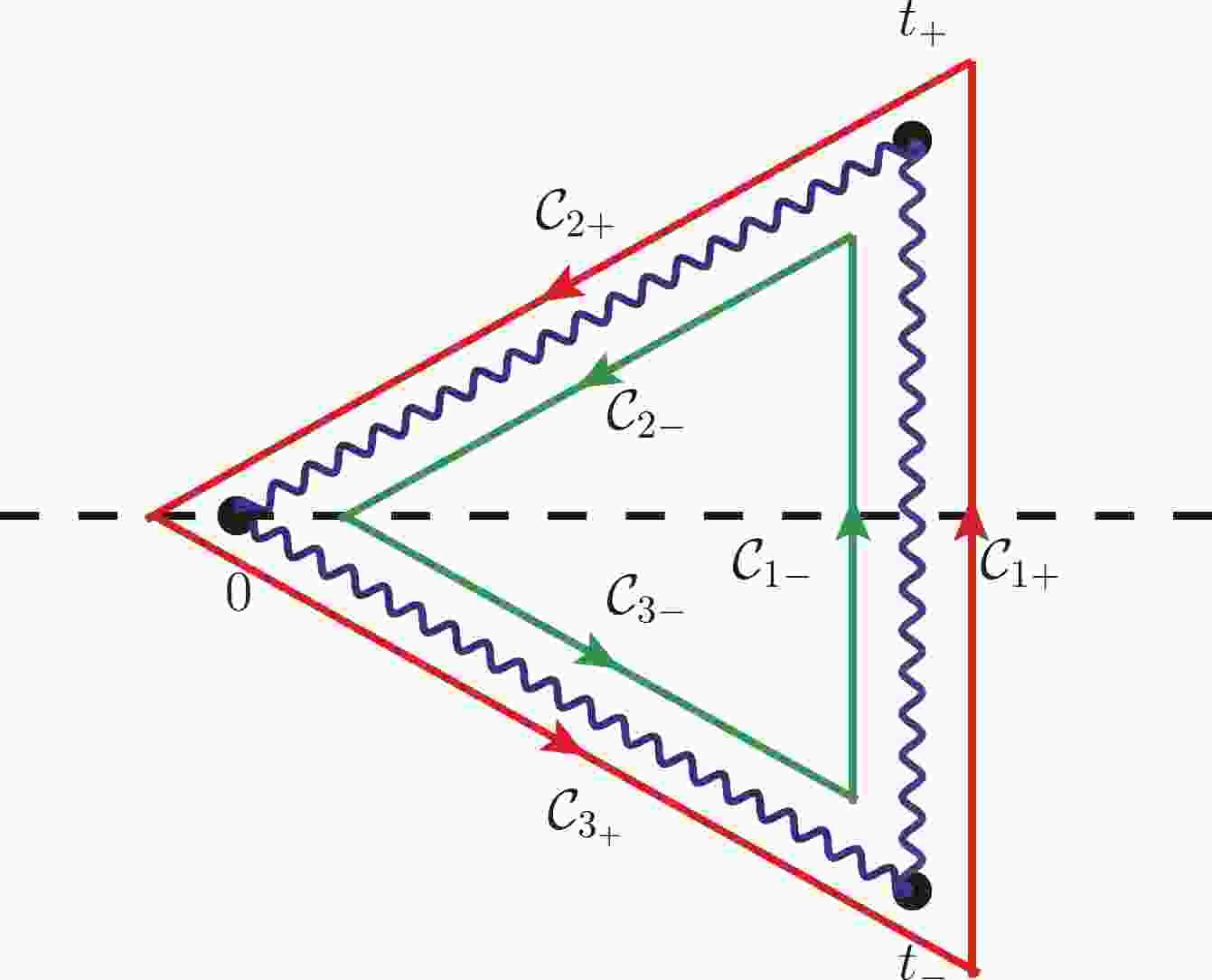
$ t_+ $ and$ t_- $ , and the branch cuts for the two logarithms to be the line segments between$ 0 $ and$ t_\pm $ , respectively. These branch cuts are depicted as the wiggly lines in Fig. 1, together with several paths$ C_{i\pm} $ thatt lie infinitesimally close to the cuts. We define the square root following the convention that$ \sqrt{(t-t_+)(t-t_-)} \to t $ when$ t \to \infty $ .
Figure 1. (color online) Branch cuts and integration paths for
$ M_{N,N-1} $ with even N.We select the integration path in Eq. (39) to along the line segment
$ {\cal{C}}_{1+} $ , and express the integral as$ M_{N,N-1} = -\frac{1}{4\pi} \left[ \int_{{\cal{C}}_{1+}} I(t) \, {\rm d}t - \int_{{\cal{C}}_{1-}} I(t) \, {\rm d}t \right] , $

(41) where we have used the characteristic that the values of
$ I(t) $ on$ {\cal{C}}_{1\pm} $ differ by a sign. Since no other singularities exist in the complex t plane (including$ \infty $ ), we may deform the paths as long as we do not go across the branch cuts. Hence, we know that$ \begin{aligned}[b] M_{N,N-1} =& \frac{1}{4\pi} \left[ \int_{{\cal{C}}_{2+}} I(t) \, {\rm d}t - \int_{{\cal{C}}_{2-}} I(t) \, {\rm d}t \right] \\ & + \frac{1}{4\pi} \left[ \int_{{\cal{C}}_{3+}} I(t) \, {\rm d}t - \int_{{\cal{C}}_{3-}} I(t) \, {\rm d}t \right]. \end{aligned} $

(42) On the paths
$ {\cal{C}}_{2+} $ and$ {\cal{C}}_{2-} $ , a$2\pi {\rm i}$ difference results from the first logarithm in Eq. (40). A similar difference of$-2\pi {\rm i}$ resulting from the second logarithm occurs between$ {\cal{C}}_{3+} $ and$ {\cal{C}}_{3-} $ . Therefore, we obtain$ \begin{aligned}[b] dM_{N,N-1} = &-\frac{\rm i}{2} \, d\int_0^{t_+} \frac{{\rm d}t}{\sqrt{(t-t_+)(t-t_-)}} \\ & - \frac{\rm i}{2} \, d\int_0^{t_-} \frac{{\rm d}t}{\sqrt{(t-t_+)(t-t_-)}} \\ = &-{\rm i} \, d\log \frac{\sqrt{r_+} - \sqrt{r_-}}{\sqrt{r_+} + \sqrt{r_-}} \, . \end{aligned} $

(43) Note that with the above convention, we obtain
$\begin{aligned}[b]& \int_{r_-}^{r_+} \frac{{\rm d}z_N}{z_N} \frac{\sqrt{\widetilde{G}_N}}{\sqrt{G_N({\bf{0}}',z_N)}}\\ =& \int_{t_-}^{t_+} \frac{{\rm d}t}{\sqrt{(t-t_+)(t-t_-)}} = {\rm i} \pi \, .\end{aligned} $

(44) We can now express the roots
$ r_\pm $ in terms of Gram determinants. The result can be expressed as$ dM_{N,N-1} = \frac{\rm i}{2} \, d\log \frac{\widetilde{B}_{N}-\sqrt{-\widetilde{G}_{N} {\cal{K}}_{N-1}}}{\widetilde{B}_{N}+\sqrt{-\widetilde{G}_{N} {\cal{K}}_{N-1}}} \, , $

(45) where the definitions of
$ \widetilde{B}_{N} $ ,$ \widetilde{G}_{N} $ , and$ {\cal{K}}_{N-1} $ are similar as before. Hence, we can express the letter in$ dM_{N,N-1} $ (for even N) as$ W_{N,N-1}(\vec{x}) = \frac{\widetilde{B}_{N}-\sqrt{-\widetilde{G}_{N} {\cal{K}}_{N-1}}}{\widetilde{B}_{N}+\sqrt{-\widetilde{G}_{N} {\cal{K}}_{N-1}}} \, . $

(46) As mentioned earlier, we do not require to consider the divergent case
$ \widetilde{G}_{N-1}=0 $ or the trivial case$ \widetilde{G}_N=0 $ here. -
As in the previous subsection, we consider the dependence of the derivative of
$ g_N $ on sub-sectors with$ N-2 $ propagators. Without loss of generality, we cut on the variables$ {\boldsymbol{z}}'=\{z_1,\ldots,z_{N-2}\} $ . Now, we remain with two sub-sectors with$ N-1 $ propagators: one with$ {\boldsymbol{z}}',z_{N-1} $ and the other with$ {\boldsymbol{z}}',z_{N} $ . We use a superscript to distinguish these two, and the differential equation then becomes$ \begin{aligned}[b] d\tilde{g}_{N} =& \epsilon \Big( dM_{N} \, \tilde{g}_{N} + dM_{N,N-1}^{(1)} \, \tilde{g}_{N-1}^{(1)} \\& + dM_{N,N-1}^{(2)} \, \tilde{g}_{N-1}^{(2)} + dM_{N,N-2} \, \tilde{g}_{N-2} \Big) \, , \end{aligned} $

(47) where we have suppressed the arguments of the functions for simplicity.
-
If N is an odd number, assuming convergence and expanding the integrands, we obtain
$ \begin{aligned}[b] d\int_{\cal{C}} \frac{{\rm d}z_{N-1}}{z_{N-1}}\frac{{\rm d}z_N}{z_N} =& 4\pi \, dM_{N,N-2} \\ &+ 2 \, dM_{N,N-1}^{(1)} \int_{r_-^{(1)}}^{r_+^{(1)}} \frac{{\rm d}z_{N-1}}{z_{N-1}} \frac{\sqrt{\widetilde{G}_{N-1}^{(1)}}}{\sqrt{G_{N-1}^{(1)}({\bf{0}}',z_{N-1})}} \\& + 2 \, dM_{N,N-1}^{(2)} \int_{r_-^{(2)}}^{r_+^{(2)}} \frac{{\rm d}z_N}{z_N} \frac{\sqrt{\widetilde{G}_{N-1}^{(2)}}}{\sqrt{G_{N-1}^{(2)}({\bf{0}}',z_N)}} \,, \end{aligned} $

(48) where the domain
$ {\cal{C}} $ is determined by$ G_N({\bf{0}}',z_{N-1},z_N)\geq 0 $ , and$ r_{\pm}^{(i)} $ are the two roots of the polynomial$ G_{N-1}^{(i)}({\bf{0}}',z) $ .The two integrals on the right-hand side can be easily performed using Eq. (35), and we obtain
$ dM_{N,N-2} = dI_{N,N-2} - \frac{\rm i}{2} \left( dM_{N,N-1}^{(1)} + dM_{N,N-1}^{(2)} \right)\, , $

(49) where
$ I_{N,N-2} $ is the double integral:$ I_{N,N-2} = \frac{1}{4\pi} \int_{\cal{C}} \frac{{\rm d}z_{N-1}}{z_{N-1}}\frac{{\rm d}z_N}{z_N} \, . $

(50) The integration domain
$ {\cal{C}} $ is controlled by the positivity of the polynomial$ \begin{aligned}[b] G_N({\bf{0}}',z_{N-1}, z_N) =& -\frac{1}{4} {\cal{K}}_{N-1} z_N^2 - B_N({\bf{0}}',z_{N-1},0) \, z_N \\ & + G_N({\bf{0}}',z_{N-1},0) \, . \end{aligned} $

(51) The integration over
$ z_N $ can be easily performed to yield$ \begin{aligned}[b] I_{N,N-2} =& \frac{1}{4\pi} \int_{r_{N-1,-}}^{r_{N-1,+}} I(z_{N-1}) \, {\rm d}z_{N-1} \\ \equiv& \frac{1}{4\pi} \int_{r_{N-1,-}}^{r_{N-1,+}} \frac{{\rm d}z_{N-1}}{z_{N-1}} \\ & \times \log \frac{B_N({\bf{0}}',z_{N-1},0) - \sqrt{\Delta(z_{N-1})}}{B_N({\bf{0}}',z_{N-1},0) + \sqrt{\Delta(z_{N-1})}} \,, \end{aligned} $

(52) where
$ r_{N-1,\pm} $ are the two roots of the polynomial$ G_{N-1}^{(1)}({\boldsymbol{z}}',z_{N-1}) = G(l,p_1,\ldots,p_{E-1}) \, , $

(53) and
$ \begin{aligned}[b] \Delta(z_{N-1}) = &\left[ B_N({\bf{0}}',z_{N-1},0) \right]^2 + {\cal{K}}_{N-1} G_N({\bf{0}}',z_{N-1},0) \\ =& {\cal{K}}_N G_{N-1}^{(1)}({\bf{0}}',z_{N-1}) \,. \end{aligned} $

(54) We are now interested in the singularities of the integrand
$ I(z_{N-1}) $ in Eq. (52). Two poles exist, at$ 0 $ and$ \infty $ , respectively. There is a branch cut between$ r_{N-1,-} $ and$ r_{N-1,+} $ for the square root. There is also a branch cut between$ R_{N-1,-} $ and$ R_{N-1,+} $ for the logarithm, where$ R_{N-1,\pm} $ are the two roots of the polynomial$ G_N({\bf{0}}',z_{N-1},0) $ . These singularities are depicted in Fig. 2. We define the integral path of Eq. (52) to be the upper half of the contour$ {\cal{C}}_1 $ . Hence, we obtain
Figure 2. (color online) Branch cuts and integration paths for
$ M_{N,N-2} $ with odd N.$ \begin{aligned}[b] I_{N,N-2} =& \frac{1}{8\pi} \int_{{\cal{C}}_1} I(z_{N-1}) \, {\rm d}z_{N-1} \\ =& -\frac{1}{8\pi} \int_{{\cal{C}}_2+{\cal{C}}_3+{\cal{C}}_4} I(z_{N-1}) \, {\rm d}z_{N-1} \,. \end{aligned} $

(55) The integration around
$ {\cal{C}}_3 $ is simply$ (-2\pi{\rm i}) $ multiplying the residue at$ z_{N-1} = 0 $ , i.e.,$ \begin{aligned}[b] -\frac{1}{8\pi} \, d\int_{{\cal{C}}_3} I(z_{N-1}) \, {\rm d}z_{N-1} =& \frac{\rm i}{4} \, d\log\frac{\widetilde{B}_N - \sqrt{ {\cal{K}}_N \widetilde{G}_{N-1}^{(1)}}}{\widetilde{B}_N + \sqrt{ {\cal{K}}_N \widetilde{G}_{N-1}^{(1)}}} \\ = &\frac{\rm i}{2} dM_{N,N-1}^{(1)} \,. \end{aligned} $

(56) On the two sides of
$ {\cal{C}}_2 $ , the logarithm differs by$2\pi {\rm i}$ , and$ \begin{aligned}[b]&-\frac{1}{8\pi} \, d\int_{{\cal{C}}_2} I(z_{N-1}) \, {\rm d}z_{N-1} = \frac{\rm i}{4} \, d\log\frac{R_{N-1,+}}{R_{N-1,-}} \\ = &\frac{\rm i}{4} \, d\log\frac{\widetilde{B}_N - \sqrt{ {\cal{K}}_N \widetilde{G}_{N-1}^{(2)}}}{\widetilde{B}_N + \sqrt{ {\cal{K}}_N \widetilde{G}_{N-1}^{(2)}}} = \frac{\rm i}{2} dM_{N,N-1}^{(2)} \,. \end{aligned} $

(57) From the above, we observe that the genuine contribution to
$ dM_{N,N-2} $ results only from the integration along$ {\cal{C}}_4 $ . For that, we must investigate the behavior of the logarithm in Eq. (52) in the limit$ z_{N-1} \to \infty $ . We first note that$ G_{N-1}^{(1)}({\bf{0}}',z_{N-1}) \sim - {\cal{K}}_{N-2} z_{N-1}^2 / 4 $ in that limit. For$ B_N({\bf{0}}',z_{N-1},0) $ , it is a linear function of$ z_{N-1} $ , and the coefficient can be extracted as$ \begin{aligned}[b] &\frac{\partial B_N({\bf{0}}',z_{N-1},0)}{\partial z_{N-1}} \\ =& \frac{\partial G(l,p_1,\ldots,p_{E-1};\, p_E,p_1,\ldots,p_{E-1})}{\partial z_{N-1}} \\ =& \frac{\partial l \cdot p_E}{\partial z_{N-1}}\frac{\partial G(l,p_1,\ldots,p_{E-1};\, p_E,p_1,\ldots,p_{E-1})}{\partial l \cdot p_E} \\ & + \frac{\partial l \cdot p_{E-1}}{\partial z_{N-1}}\frac{\partial G(l,p_1,\ldots,p_{E-1};\, p_E,p_1,\ldots,p_{E-1})}{\partial l\cdot p_{E-1}} \\ = &\frac{1}{2} G(p_1,\ldots,p_{E-1};\, p_1,\ldots,p_{E-1}) \\ & + \frac{1}{2} G(p_1,\ldots,p_{E-2},p_{E-1};\, p_1,\ldots,p_{E-2},p_{E}) \\ =& \frac{1}{2}G(p_1,\ldots,p_{E-2},p_{E-1};\, p_1,\ldots,p_{E-2},p_{E-1}+p_E) \, . \end{aligned} $

(58) Hence, we obtain
$ \begin{aligned}[b] dM_{N,N-2} =& -\frac{1}{8\pi} \, d\int_{{\cal{C}}_4} I(z_{N-1}) \, {\rm d}z_{N-1} \\ =& \frac{\rm i}{4} d\log \frac{C_N - \sqrt{- {\cal{K}}_N {\cal{K}}_{N-2}}}{C_N + \sqrt{- {\cal{K}}_N {\cal{K}}_{N-2}}} \, , \end{aligned} $

(59) where
$ C_N = G(p_1,\ldots,p_{E-2},p_{E-1};\, p_1,\ldots,p_{E-2},p_{E-1}+p_E) \, . $

(60) The letter
$ W_{N,N-2} $ can be readily read off. Note that the Gram determinants in this letter only involve external momenta. Hence, the letter has a well-defined limit when$ \widetilde{G}_{N-2} = 0 $ and$ g_{N-2} $ is not a master. We explain the meaning of this later. -
If N is an even number, assuming no divergence, we obtain the differential equation
$ d\int_{\cal{C}} \frac{{\rm d}z_{N-1}}{z_{N-1}} \frac{{\rm d}z_N}{z_N}\frac{\sqrt{\widetilde{G}_N}}{\sqrt{G_N({\bf{0}}',z_{N-1},z_N)}} = 4\pi \, dM_{N,N-2} \,, $

(61) where the domain
$ {\cal{C}} $ is determined by$ G_N({\bf{0}}',z_{N-1},z_N) \geq 0 $ . Note that the dependence on$ g_{N-1}^{(i)} $ vanishes in this case. We select to integrate over$ z_N $ first and obtain$ \begin{aligned}[b] dM_{N,N-2} =&\frac{1}{4\pi} \, d\int_{r_{N-1,-}}^{r_{N-1,+}} \frac{{\rm d}z_{N-1}}{z_{N-1}} \frac{\sqrt{\widetilde{G}_N}}{\sqrt{G_N({\bf{0}}',z_{N-1},0)}}\end{aligned} $

$ \begin{aligned}[b] \quad\times \int_{r_{N,-}}^{r_{N,+}} \frac{{\rm d}z_N}{z_N}\frac{\sqrt{G_N({\bf{0}}',z_{N-1},0)}}{\sqrt{G_N({\bf{0}}',z_{N-1},z_N)}} \,, \end{aligned} $

(62) where
$ r_{N,\pm} $ are the two roots of the polynomial$ G_N({\bf{0}}',z_{N-1},z_N) $ with respect to$ z_N $ (treating$ z_{N-1} $ as a constant). Consequently, the integration range of$ z_{N-1} $ is determined by the discriminant Δ of$ G_N({\bf{0}}',z_{N-1},z_N) $ (with respect to the variable$ z_N $ ). Expressing$\Delta = {\cal{K}}_4 G_{N-1}^{(1)}\times ({\bf{0}}',z_{N-1})$ , we know that the bounds$ r_{N-1,\pm} $ are simply the two roots of the polynomial$ G_{N-1}^{(1)}({\bf{0}}',z_{N-1}) $ . Here, we define$ \begin{aligned}[b] G_{N-1}^{(1)}({\boldsymbol{z}}',z_{N-1}) =& G(l,p_1,\ldots,p_{E-1}) \, , \\ G_{N-1}^{(2)}({\boldsymbol{z}}',z_{N}) =& G(l,p_1,\ldots,p_{E-1}+p_E) \, .\end{aligned} $

(63) The integration over
$ z_N $ can be performed using Eq. (35). We then obtain$ dM_{N,N-2} = \frac{\rm i}{4} \, dI_{N,N-2} \,, $

(64) where
$ I_{N,N-2} = \int_{r_{N-1,-}}^{r_{N-1,+}} \frac{{\rm d}z_{N-1}}{z_{N-1}} \frac{\sqrt{\widetilde{G}_N}}{\sqrt{G_N({\bf{0}}',z_{N-1},0)}} \, , $

(65) where
$ r_{N-1,\pm} $ are the two roots of$ G_{N-1}^{(1)}({\bf{0}}',z_{N-1}) $ . We denote the two roots of$ G_N({\bf{0}}',z_{N-1},0) $ as$ R_{N-1,\pm} $ . We can then write$ G_N({\bf{0}}',z_{N-1},0) = -\frac{1}{4} {\cal{K}}_{N-1}^{(2)} (z_{N-1}-R_{N-1,+})(z_{N-1}-R_{N-1,-}) \, , $

(66) where
$ {\cal{K}}_{N-1}^{(2)} = G(p_1,\ldots,p_{E-2},p_{E-1}+p_E) \, . $

(67) We define
$ t = \frac{1}{z_{N-1}} \, , \quad t_{\pm} = \frac{1}{r_{N-1,\mp}} \, , \quad T_{\pm} = \frac{1}{R_{N-1,\mp}} \, . $

(68) The integral can then be expressed as
$ \begin{aligned}[b] I_{N,N-2} =& \int_{t_-}^{t_+} \frac{{\rm d}t}{\sqrt{(t-T_+)(t-T_-)}} \\ =& 2 \log \frac{\sqrt{t_+-T_+} + \sqrt{t_+-T_-}}{\sqrt{t_–T_+} + \sqrt{t_–T_-}} \, . \end{aligned} $

(69) We now aim to rewrite the above expression in terms of Gram determinants. Hence, we first write
$ \begin{aligned}[b] G_N({\bf{0}}',z_{N-1},0) =& -\frac{1}{4} {\cal{K}}_{N-1}^{(2)} z_{N-1}^2 - \widetilde{B}_{N} z_{N-1} + \widetilde{G}_N \, , \\ G_{N-1}^{(1)}({\bf{0}}',z_{N-1}) =& -\frac{1}{4} {\cal{K}}_{N-2} z_{N-1}^2 - \widetilde{B}_{N-1}^{(1)} z_{N-1} + \widetilde{G}_{N-1}^{(1)} \, , \end{aligned} $

(70) where
$ \begin{aligned}[b] {\cal{K}}_{N-2} =& G(p_1,\ldots,p_{E-2}) \, , \\ B_{N-1}^{(1)}({\boldsymbol{z}}) =& G(l,p_1,\ldots,p_{E-2};\, p_{E-1},p_1,\ldots,p_{E-2}) \, . \end{aligned} $

(71) The roots are given by
$ \begin{aligned}[b] t_{\pm} =& \frac{\widetilde{B}_{N-1}^{(1)} \pm \sqrt{ {\cal{K}}_{N-1}^{(1)} \widetilde{G}_{N-2}}}{2\widetilde{G}_{N-1}^{(1)}} \, , \\ T_{\pm} =& \frac{\widetilde{B}_{N} \pm \sqrt{ {\cal{K}}_{N} \widetilde{G}_{N-1}^{(2)}}}{2\widetilde{G}_{N}} \, , \end{aligned} $

(72) where
$ G_{N-1}^{(2)} = G(l,p_1,\ldots,p_{E-2},p_{E-1}+p_E) \, , $

(73) and we have used the relations
$ \begin{aligned}[b] B_N^2 + {\cal{K}}_{N-1}^{(2)} G_N =& {\cal{K}}_N G_{N-1}^{(2)} \, , \\ \left( B_{N-1}^{(1)} \right)^2 + {\cal{K}}_N G_{N-1}^{(1)} = &{\cal{K}}_{N-1}^{(1)} G_{N-2} \, . \end{aligned} $

(74) We can now employ the geometric representations of the Gram determinants in Eq. (31) to simplify the expressions. Let
$ l^\star $ be the solution to$ {\boldsymbol{z}}=0 $ ; we are interested in the components of$ l^\star $ ,$ p_{E-1} $ and$ p_{E-1}+p_E $ orthogonal to the subspace spanned by$ \{p_1,\ldots,p_{E-2}\} $ . For convenience, we denote these components as$ k^\mu $ (for$ l^\star $ ),$ p^\mu $ (for$ p_{E-1} $ ) and$ q^\mu $ (for$ p_{E-1}+p_E $ ). We note that$ k^\mu $ is time-like, while$ p^\mu $ and$ q^\mu $ are space-like. Hence, we can define the norms$ |k| = \sqrt{k^2} $ ,$ |p| = \sqrt{-p^2} $ , and$ |q| = \sqrt{-q^2} $ . We further denote the components of$ k^\mu $ and$ p^\mu $ perpendicular to q as$ k_\perp^\mu $ and$ p_\perp^\mu $ , respectively, and define the corresponding norms as$ |k_\perp| $ and$ |p_\perp| $ . We can finally write$ t_{\pm} = \frac{\sinh(\eta_1) \pm {\rm i}}{2 |k| |p| \cosh^2(\eta_1)} \, , \quad T_{\pm} = \frac{\sinh(\eta_2) \pm {\rm i}}{2 |k_{\perp}| |p_\perp| \cosh^2(\eta_2)} \, , $

(75) where
$ \eta_1 $ is the hyperbolic angle between k and p, and$ \eta_2 $ is the hyperbolic angle between$ k_\perp $ and$ p_\perp $ . It will be convenient to define the imaginary angle$\theta_{kp} \equiv \pi/2 - {\rm i}\eta_1$ such that$ \cosh(\eta_1) = \sin\theta_{kp} $ and${\rm i}\, \sinh(\eta_1) = \cos\theta_{kp}$ ; similarly,$\theta_{kp,\perp q} \equiv \pi/2 - {\rm i}\eta_2$ .We use
$ \theta_{pq} $ to denote the angle between p and q and define ξ as the hyperbolic angle between k and q (with the corresponding imaginary angle$\theta_{kq} \equiv \pi/2 - {\rm i}\xi$ ). We then obtain the relations$ \begin{aligned}[b] \quad |p_\perp| =& |p| \sin\theta_{pq} \, , \quad |k_\perp| = |k| \sin\theta_{kq} \, , \\ \cos\theta_{kp} =& \cos\theta_{kq} \cos\theta_{pq} + \cos\theta_{kp,\perp q} \sin\theta_{kq} \sin\theta_{pq} \, . \end{aligned} $

(76) Thus,
$ t_{\pm} - T_{\pm} \equiv \frac{P_{\pm\pm}}{2|k_\perp| |p_\perp| \sin^2\theta_{kp} \sin^2\theta_{kp,\perp q}} \, , $

(77) where
$ \begin{aligned}[b] P_{\pm\pm} =& (-{\rm i}\cos\theta_{kp} \pm {\rm i}) \sin^2\theta_{kp,\perp q} \sin\theta_{pq} \sin\theta_{kq} \\ &- (-{\rm i}\cos\theta_{kp,\perp q} \pm {\rm i}) \sin^2\theta_{kp} \, .\end{aligned} $

(78) Substituting the relation (76), we may express the functions
$ P_{\pm\pm} $ as$ \begin{aligned}[b] P_{++} =& -8 {\rm i} \, \sin^2\left( \frac{\theta_{kp}}{2} \right) \cos^2\left( \frac{\theta_{kq}+\theta_{pq}}{2} \right) \sin^2\left( \frac{\theta_{kp,\perp q}}{2} \right) , \\ P_{+-} =& 8 {\rm i}\, \sin^2\left( \frac{\theta_{kp}}{2} \right) \cos^2\left( \frac{\theta_{kq}-\theta_{pq}}{2} \right) \cos^2\left( \frac{\theta_{kp,\perp q}}{2} \right) , \\ P_{-+} = &-8 {\rm i}\, \cos^2\left( \frac{\theta_{kp}}{2} \right) \sin^2\left( \frac{\theta_{kq}+\theta_{pq}}{2} \right) \sin^2\left( \frac{\theta_{kp,\perp q}}{2} \right) , \\ P_{ - - } =& 8 {\rm i} \, \cos^2\left( \frac{\theta_{kp}}{2} \right) \sin^2\left( \frac{\theta_{kq}-\theta_{pq}}{2} \right) \cos^2\left( \frac{\theta_{kp,\perp q}}{2} \right) . \end{aligned} $

(79) Using trigonometry identities together with the relations
$ \begin{aligned}[b]\cos\theta_{pq} =& \cos\theta_{kp} \cos\theta_{kq} + \cos\theta_{pq,\perp k} \sin\theta_{kp} \sin\theta_{kq} \, , \\ \sin\theta_{pq} =& \sin\theta_{pq,\perp k} \, \frac{\sin\theta_{kp}}{\sin\theta_{kp,\perp q}} \, , \end{aligned} $

(80) we obtain a surprisingly simple result:
$ I_{N,N-2} = 2 \log {\rm e}^{-{\rm i} \theta_{pq,\perp k}} = \log \frac{\cos\theta_{pq,\perp k} - {\rm i} \sin\theta_{pq,\perp k}}{\cos\theta_{pq,\perp k} + {\rm i} \sin\theta_{pq,\perp k}} \, , $

(81) where
$ \theta_{pq,\perp k} $ is the angle between$ p_{\perp k} $ and$ q_{\perp k} $ . It is straightforward to rewrite the above expression in terms of Gram determinants, and we finally obtain$ dM_{N,N-2} = \frac{\rm i}{4} d\log \frac{\widetilde{D}_N - \sqrt{-\widetilde{G}_N\widetilde{G}_{N-2}}}{\widetilde{D}_N + \sqrt{-\widetilde{G}_N\widetilde{G}_{N-2}}} \,, $

(82) where
$ \widetilde{D}_{N} = D_N({\bf{0}}) $ and$ D_N({\boldsymbol{z}}) = G(l,p_1,\ldots,p_{E-1};l,p_1,\ldots,p_{E-1}+p_E) \, . $

(83) -
In the convergent case,
$ dg_{N} $ cannot depend on$ g_{N-3} $ or integrals with even fewer propagators. For odd N, this can be easily observed from the powers of$ \epsilon $ in Eq. (11). However, for even N,$ dg_{N} $ and$ g_{N-3} $ are multiplied by the same power of$ \epsilon $ in the differential equations. Subsequently, we must examine the three-fold integrals appearing in the differential equations under the$ (N-3) $ -cut. The first two folds can be performed using the calculations in Section III.C.2, and the last fold can be studied similar to those in Section III.C.1. Finally, we can arrive at the conclusion that$ dM_{N,N-3}=0 $ in the convergent case. However, note that such dependence can be present in the divergence cases, as discussed in the next section. -
We now consider the scenario in which some cut integrals become divergent and we cannot perform a Taylor expansion for the integrands. As discussed earlier, this occurs when certain Gram determinants vanish under the maximal cut, and the corresponding integrals are reducible to lower sectors. A classical example is the massless three-point integral that can be reduced to two-point integrals. Reducible higher-point integrals can occur with specific configurations of external momenta, which appear, e.g., at boundaries of differential equations or in some effective field theories. Divergent cut integrals can have two types of consequences, which we discuss in the following.
-
We consider the dependence of
$ dg_{N} $ on$ g_{N-2} $ when$ g_{N-1}^{(1)} $ is reducible, where N is even. Following the derivation in Section III.C.2, we observe that now one of$ r_{N-1,\pm} $ is zero and$ G_{N-1}^{(1)}({\bf{0}}',0) = 0 $ . Hence, integration over$ z_{N-1} $ is divergent and we cannot perform Taylor expansion of the integrand in$ \epsilon $ . Moreover, we observe that the entry$ dM_{N,N-2} $ obtained in Section III.C.2 is divergent. To proceed, we can maintain the regulator in the differential equation:$ \begin{aligned}[b] &d\int_{\cal{C}} \frac{{\rm d}z_{N-1}}{z_{N-1}} \frac{{\rm d}z_N}{z_N} \frac{\sqrt{\widetilde{G}_N}}{\sqrt{G_N({\bf{0}}',z_{N-1},z_N)}} \left[-\frac{ {\cal{K}}_N}{G_N({\bf{0}}',z_{N-1},z_N)}\right]^\epsilon \\ =& \epsilon \, dM_{N} \int_{\cal{C}} \frac{{\rm d}z_{N-1}}{z_{N-1}} \frac{{\rm d}z_N}{z_N} \end{aligned} $

$ \begin{aligned}[b] \quad & \times \frac{\sqrt{\widetilde{G}_N}}{\sqrt{G_N({\bf{0}}',z_{N-1},z_N)}} \left[-\frac{ {\cal{K}}_N}{G_N({\bf{0}}',z_{N-1},z_N)}\right]^\epsilon \\& + 4\pi \, dM_{N,N-2}^\star \left(-\frac{ {\cal{K}}_{N-2}}{\widetilde{G}_{N-2}}\right)^\epsilon + {\cal{O}}(\epsilon) \,, \end{aligned} $

(84) where
$ dM_{N,N-2}^\star $ denotes the entry in the divergent case. Note that$ g_{N-1}^{(1)} $ is not a master integral and does not contribute to the right-hand side, while the last$ {\cal{O}}(\epsilon) $ denotes a suppressed contribution from another$ (N-1) $ -point integral$ g_{N-1}^{(2)} $ . Here, we assume that$ G_{N-1}^{(2)}({\bf{0}}',0) $ is non-zero and the integration over$ z_N $ is convergent for$ \epsilon \to 0 $ .We now must perform Laurent expansions of the integrands in terms of distributions. We write
$ \begin{aligned}[b] G_{N-1}^{(1)}({\bf{0}}',z_{N-1}) =& \frac{1}{4} {\cal{K}}_{N-2} z_{N-1} \, (t - z_{N-1}) \, , \\ t =& - \frac{4\widetilde{B}_{N-1}^{(1)}}{ {\cal{K}}_{N-2}} \, . \end{aligned} $

(85) We can then use
$ \int_0^t \frac{{\rm d}z}{z^{1+\epsilon}} \, f(z) = -\frac{t^{-\epsilon}}{\epsilon} \, f(0) + \int_0^t \frac{{\rm d}z}{z^{1+\epsilon}} \left[ f(z) - f(0) \right] , $

(86) to perform the series expansion. In particular, we obtain
$ \begin{aligned}[b]&\int_{\cal{C}} \frac{{\rm d}z_{N-1}}{z_{N-1}} \frac{{\rm d}z_N}{z_N} \frac{\sqrt{\widetilde{G}_N}}{\sqrt{G_N({\bf{0}}',z_{N-1},z_N)}} \left[-\frac{ {\cal{K}}_N}{G_N({\bf{0}}',z_{N-1},z_N)}\right]^\epsilon \\ =& {\rm i}\pi \int_0^t \frac{{\rm d}z_{N-1}}{z_{N-1}^{1+\epsilon}} \frac{\sqrt{\widetilde{G}_N}}{\sqrt{G_N({\bf{0}}',z_{N-1},0)}} \\&\times \left[ 1 + \epsilon \, h(z_{N-1}) + {\cal{O}}(\epsilon^2) \right] \\ =& {\rm i}\pi \Bigg[ -\frac{1}{\epsilon} + \log(t) - h(0) \\& + \int_0^t \frac{{\rm d}z_{N-1}}{z_{N-1}} \left( \frac{\sqrt{\widetilde{G}_N}}{\sqrt{G_N({\bf{0}}',z_{N-1},0)}} - 1 \right) \Bigg] + {\cal{O}}(\epsilon) \, , \end{aligned} $

(87) where the function
$ h(z_{N-1}) $ results from the expansion in$ \epsilon $ after integrating over$ z_N $ . When$ z_{N-1} \to 0 $ , it reduces to$ h(0) = \log \left( \frac{4 {\cal{K}}_{N-1}^{(1)}}{\widetilde{B}_{N-1}^{(1)}} \right) + 4\log(2) \, . $

(88) The last integral in Eq. (87) can be obtained by obtaining the limit
$ \widetilde{G}_{N-1}^{(1)} \to 0 $ in the difference between Eq. (82) and a simple integral of$ 1/z_{N-1} $ :$ \begin{aligned}[b]& \int_0^t \frac{{\rm d}z_{N-1}}{z_{N-1}} \left( \frac{\sqrt{\widetilde{G}_N}}{\sqrt{G_N({\bf{0}}',z_{N-1},0)}} - 1 \right) \\ =& \lim\limits_{\widetilde{G}_{N-1}^{(1)} \to 0} \left( \log\frac{\widetilde{D}_{N} - \sqrt{-\widetilde{G}_{N} \widetilde{G}_{N-2}}}{\widetilde{D}_{N} + \sqrt{-\widetilde{G}_{N} \widetilde{G}_{N-2}}} - \log\frac{\widetilde{B}_{N-1}^{(1)} +\sqrt{\widetilde{G}_{N-2} {\cal{K}}_{N-1}^{(1)}}}{\widetilde{B}_{N-1}^{(1)} -\sqrt{\widetilde{G}_{N-2} {\cal{K}}_{N-1}^{(1)}}} \right) \,. \end{aligned} $

(89) Using the relations
$ \begin{aligned}[b] -G_{N} G_{N-2}=&D_{N}^2-G_{N-1}^{(1)}G_{N-1}^{(2)} \, , \\ G_{N-2} {\cal{K}}_{N-1}^{(1)}=&\left(B_{N-1}^{(1)}\right)^2+G_{N-1}^{(1)} {\cal{K}}_{N-2} \, , \end{aligned} $

(90) we can simplify the expression and obtain
$ \int_0^t \frac{{\rm d}z_{N-1}}{z_{N-1}} \left( \frac{\sqrt{\widetilde{G}_N}}{\sqrt{G_N({\bf{0}}',z_{N-1},0)}} - 1 \right) = \log \frac{\widetilde{G}_N {\cal{K}}_{N-2}}{ {\cal{K}}_{N-1}^{(1)}\widetilde{G}_{N-1}^{(2)} } \, . $

(91) Now, we can combine everything, and we observe that in the divergent case (for even N),
$ W_{N,N-2}^\star = \frac{\widetilde{G}_{N-2} \, {\cal{K}}_N}{ {\cal{K}}_{N-1}^{(1)} \, \widetilde{G}_{N-1}^{(2)}} \, . $

(92) Comparing to Eq. (92), we note that the letter in the divergent case is simpler (without square roots) than that in the convergent case. Interestingly, this simple letter can be obtained without using the tedious calculation above. We observe that in the divergent case
$ \widetilde{G}_{N-1}^{(1)} \to 0 $ , we have the relation$ \tilde{g}_{N-1}^{(1)} = -\frac{1}{2} \tilde{g}_{N-2} \, . $

(93) This hints that we should combine
$ dM_{N,N-1}^{(1)} $ and$ dM_{N,N-2} $ to obtain$ dM_{N,N-2}^\star $ :$ \begin{aligned}[b] dM_{N,N-2}^{\star} =& \lim\limits_{\widetilde{G}_{N-1}^{(1)}\to 0} \left( -\frac{1}{2} dM_{N,N-1}^{(1)} + dM_{N,N-2} \right) \\ =& \frac{\rm i}{4} \lim\limits_{\widetilde{G}_{N-1}^{(1)} \to 0} \left( \log\frac{\widetilde{D}_{N} - \sqrt{-\widetilde{G}_{N} \widetilde{G}_{N-2}}}{\widetilde{D}_{N} + \sqrt{-\widetilde{G}_{N} \widetilde{G}_{N-2}}} \right.\\&-\left. \log\frac{\widetilde{B}_{N}^{(1)} -\sqrt{-\widetilde{G}_{N} {\cal{K}}_{N-1}^{(1)}}}{\widetilde{B}_{N}^{(1)} +\sqrt{-\widetilde{G}_{N} {\cal{K}}_{3}^{(N)}}} \right) \,. \end{aligned} $

(94) Using the relations in Eq. (90) as well as
$ -G_{N} {\cal{K}}_{N-1}^{(1)}=\left(B_{N}^{(1)}\right)^2+G_{N-1}^{(1)} {\cal{K}}_{N} \, , $

(95) we can easily arrive at Eq. (92).
Further divergences may occur if
$ \widetilde{G}_{N-1}^{(2)} = 0 $ in Eq. (92). In this case, both$ g_{N-1}^{(1)} $ and$ g_{N-1}^{(2)} $ are reducible to lower-point integrals. The corresponding letter can be obtained by including$ dM_{N,N-1}^{(2)} $ , but we do not elaborate on the calculation here. We finally note that the above considerations can also be applied to the N-odd cases, although here$ g_{N-1}^{(i)} $ can only be reducible for specific configurations of external momenta. We discuss similar scenarios in the next subsection. -
In the convergent case, we have observed that
$ dg_{N} $ can only depend on$ g_N $ ,$ g_{N-1}^{(i)} $ , and$ g_{N-2}^{(i)} $ . This picture changes in the divergent case when one of$ g_{N-2}^{(i)} $ is reducible, and$ dg_{N} $ may develop dependence on some$ (N-3) $ -point integrals. As a practical example, we consider the dependence of 5-point integrals on 2-point ones. According to Eq. (17), we obtain$ \begin{aligned}[b] d\tilde{g}_5 =& \epsilon \, dM_5 \, \tilde{g}_5 + \epsilon \sum\limits_i dM_{5,4}^{(i)} \, \tilde{g}_4^{(i)} + \epsilon \sum\limits_i dM_{5,3}^{(i)} \, \tilde{g}_3^{(i)} \\ & + \epsilon \, dM_{5,2} \, \tilde{g}_2 \, , \end{aligned} $

(96) where the cut on
$ z_1 $ and$ z_2 $ is imposed. Using Eq. (11), we arrive at$ \begin{aligned}[b] dM_{5,2} + {\cal{O}}(\epsilon) =& \frac{\epsilon}{8\pi} \, dI_{5,2}(\epsilon) - \frac{\epsilon}{4\pi} \sum\limits_{i=3}^5 dM_{5,4}^{(i)} \, I_{4,2}^{(i)}(\epsilon) \\ &- \frac{\epsilon}{2} \sum\limits_{i=3}^5 dM_{5,3}^{(i)} \, I_{3,2}^{(i)}(\epsilon) \, , \end{aligned} $

(97) where
$ \begin{aligned}[b] I_{5,2}(\epsilon) =& \int \frac{{\rm d}z_3}{z_3} \frac{{\rm d}z_4}{z_4} \frac{{\rm d}z_5}{z_5} \left( -\frac{ {\cal{K}}_5}{G_5(0,0,z_3,z_4,z_5)} \right)^\epsilon , \\ I_{4,2}^{(i)}(\epsilon) =& \int \frac{{\rm d}z_j}{z_j} \frac{{\rm d}z_k}{z_k} \frac{\sqrt{G_4^{(i)}(0,0,0,0)}}{\sqrt{G_4^{(i)}(0,0,z_j,z_k)}} \\& \times \left( -\frac{ {\cal{K}}_4^{(i)}}{G_4^{(i)}(0,0,z_j,z_k)} \right)^\epsilon , \\ I_{3,2}^{(i)}(\epsilon) =& \int \frac{{\rm d}z_i}{z_i} \left( -\frac{ {\cal{K}}_3^{(i)}}{G_3^{(i)}(0,0,z_i)} \right)^\epsilon , \end{aligned} $

(98) where
$ j<k $ and$ j,k \neq i $ . We note that each term on the right-hand side of Eq. (97) has a factor of$ \epsilon $ . Therefore, the term can only contribute if the integral is divergent in the limit$ \epsilon \to 0 $ . For that to occur, at least one of$ G_3^{(i)}(0,0,0) $ must vanish. For simplicity, we assume$ G_3^{(3)}(0,0,0) = 0 $ , while the other two$ G_3^{(i)}(0,0,0) $ 's are non-zero. Generally, it is clear that the$ I_{3,2}^{(i)}(\epsilon) $ terms do not contribute since they are either zero or non-divergent. The integrals$ I_{4,2}^{(4)}(\epsilon) $ and$ I_{4,2}^{(5)}(\epsilon) $ are similar to Eq. (87) with the result$-{\rm i}\pi/\epsilon + {\cal{O}}(\epsilon^0)$ . Therefore, we only require to address the divergent part of$ I_{5,2}(\epsilon) $ :$ \begin{aligned}[b] I_{5,2}(\epsilon) =& \int \frac{{\rm d}z_3}{z_3} \frac{{\rm d}z_4}{z_4} \left[ \Delta(z_3,z_4) \right]^{-\epsilon} \\& \times\log\frac{B_5^{(5)}(0,0,z_3,z_4,0) - \sqrt{\Delta(z_3,z_4)}}{B_5^{(5)}(0,0,z_3,z_4,0) + \sqrt{\Delta(z_3,z_4)}} + {\cal{O}}(\epsilon^0) \, , \end{aligned} $

(99) where
$ \Delta(z_3,z_4) = {\cal{K}}_5 G_{4}^{(5)}(0,0,z_3,z_4) \, . $

(100) The integration over
$ z_4 $ is similar to Eq. (52), except for the additional factor$ \Delta^{-\epsilon} $ , which regularizes the divergence as$ z_3 \to 0 $ . Since we are only interested in the leading term in$ \epsilon $ , it is equivalent to replacing this factor by$ z_3^{-\epsilon} $ . We can then expand$ z_3^{-1-\epsilon} $ in terms of distributions. Maintaining only the$ 1/\epsilon $ terms, we obtain$ \begin{aligned}[b] &dI_{5,2}(\epsilon) + {\cal{O}}(\epsilon^0)\\ =& -\frac{1}{\epsilon} d\int \frac{{\rm d}z_4}{z_4} \log\frac{B_5^{(5)}(0,0,0,z_4,0) - \sqrt{\Delta(0,z_4)}}{B_5^{(5)}(0,0,0,z_4,0) + \sqrt{\Delta(0,z_4)}} \\ =& -\frac{1}{\epsilon}\left( 2\pi {\rm i} \, dM_{5,4}^{(4)} + 2\pi {\rm i}\, dM_{5,4}^{(5)} + 4\pi \, dM_{5,3}^{(3)} \right)\, , \end{aligned} $

(101) where the second line follows from the calculation of Eq. (52). We finally arrive at
$ dM_{5,2} = -\frac{1}{2} dM_{5,3}^{(3)} = -\frac{\rm i}{8} d\log \frac{C_5 - \sqrt{- {\cal{K}}_5 {\cal{K}}_{3}}}{C_5 + \sqrt{- {\cal{K}}_5 {\cal{K}}_{3}}} , $

(102) where
$ C_5 = G(p_1,p_2,p_3,p_4;\, p_1,p_2,p_3,p_4+p_5) \, . $

(103) The result in Eq. (102) is unsurprising owing to the relation
$ g_3^{(3)}=-g_2/2 $ . Similar behaviors are observed when more than one$ \widetilde{G}_3 $ vanish. The corresponding$ dM_{5,2} $ is then a linear combination of several$ dM_{5,3} $ 's. Hence, we conclude that letters in these cases can also be obtained straightforwardly without tedious calculations.The above discussion relates the appearance of
$ dM_{N,N-3} $ to the reducibility of one or more$ g_{N-2}^{(i)} $ 's. We may consider that, if in addition, one or more$ g_{N-3}^{(i)} $ 's becomes reducible,$ dM_{N,N-4} $ can appear in the differential equations. This is impossible for integrals with generic external momenta (i.e., the E external momenta are indeed independent). However, such cases may occur at certain boundaries of kinematic configurations. When this occurs, the corresponding letters can be easily obtained using the reduction rules among the integrals, as is conducted in the previous paragraph. -
In summary, we have studied the alphabet for one-loop Feynman integrals. The alphabet governs the form of the canonical differential equations and provides important information on the analytic solution of these equations. We observe that the letters in the alphabet can be generically constructed using UT integrals in the Baikov representation under various cuts. We have first considered cases in which all the cut integrals are convergent in the limit
$ \epsilon \to 0 $ . The corresponding letters coincide with the results in [37–39], while our expressions are simpler in certain cases. We have also thoroughly studied the cases of divergent cut integrals. We observe that letters in the divergent cases can be easily obtained from the convergent cases by applying certain limits. The letters admit universal expressions in terms of various Gram determinants. We have checked our general results for several known examples and observed agreements. We have also applied our results to the complicated case of a$ 2 \to 3 $ amplitude with seven physical scales. The details of that is presented in Ref. [44].We expect that our results will be useful in many calculations of
$ 2 \to 3 $ and$ 2 \to 4 $ amplitudes, which are theoretically and/or phenomenologically interesting. It is also interesting to observe whether similar universal structures can be obtained at higher loop orders using the UT integrals in the Baikov representation of [16, 23].
Alphabet of one-loop Feynman integrals
- Received Date: 2022-03-04
- Available Online: 2022-09-15
Abstract: In this paper, we present the universal structure of the alphabet of one-loop Feynman integrals. The letters in the alphabet are calculated using the Baikov representation with cuts. We consider both convergent and divergent cut integrals and observe that letters in the divergent cases can be easily obtained from convergent cases by applying certain limits. The letters are written as simple expressions in terms of various Gram determinants. The knowledge of the alphabet enables us to easily construct the canonical differential equations of the


 DownLoad: