Study of lepton EDMs in the U(1)_X SSM

In 1964, Cronin and Fitch discovered charge conjugate and parity (CP) violation from the decays of the $ K $ meson [1], and lepton electric dipole moments (EDMs) have become a physical quantity used to probe sources of CP violation [2]. Therefore, it is important to research the EDMs of leptons. At present, the upper bound of the electron EDM is $|d^{\rm exp}_e| < 1.1 \times 10^{-29}$ e.cm at the $ 90$% confidence level [3–5], whereas that of the muon EDM is $ |d^{\rm exp}_{\mu}| < 1.8 \times 10^{-19} $ e.cm at the $ 95$% confidence level and that of the tau EDM is $ |d^{\rm exp}_{\tau}| < 1.1 \times 10^{-17} $ e.cm at the $ 95$% confidence level [6]. The sources and mechanism of CP violation have not been well explained, and scientists have been attempting to find CP violation terms in new physics beyond the SM to better explain the CP violation mechanism [7–10]. There are several CP violating phases, which can provide large contributions to the EDMs of leptons in the minimal supersymmetric extension of the standard model (MSSM) [11–14].

Owing to the deficiency of the MSSM, which cannot explain neutrino mass or solve the $ \mu $ problem, a U(1) extension of the MSSM is performed. There are two U(1) groups in the $ U(1)_X $SSM: $ U(1)_Y $ and $ U(1)_X $, and the $ U(1)_X $SSM is explored using SARAH software packages [15–17]. By adding new superfields to the MSSM, the $ U(1)_X $SSM not only obtains additional Higgs, neutrinos, and gauge fields, but corresponding superpartners that extend the neutralino and sfermion sectors. The mass $ m_{h_0} $ of the lightest CP-even Higgs [18, 19] in the $ U(1)_X $SSM is larger than its corresponding mass in the MSSM at tree order. Therefore, in the $ U(1)_X $SSM, the loop diagram correction of $ m_{h_0} $ does not need to be large.

An effective way to explore new physics beyond the standard model (SM) is through researching the MDMs [20, 21] and EDMs [22–28] of leptons. The one-loop and two-loop corrections to lepton EDMs have been well researched in the MSSM. $ d_e $ in the SM was studied independently of the model [29, 30], and the authors considered right-handed neutrinos, the neutrino see-saw mechanism, and the structure of minimal flavor violation. The results showed that when neutrinos are Majorana particles, the value of $ d_e $ will reach the upper limit of the experiment.

This paper is organized as follows: We introduce the specific form of the $ U(1)_X $SSM and its superfields in Section II. In Section III, we show the one-loop and two-loop corrections to lepton EDMs. The main content of Section IV is a numerical analysis on the dependence of lepton EDMs on $ U(1)_X $SSM parameters. We provide a summary and discussion in Section V. The appendix contains mass matrics.

The $ U(1)_X $SSM is expanded on the basis of the MSSM. $ U(1)_X $SSM superfields include three Higgs singlets $ \hat{\eta},\; \hat{\bar{\eta}},\; \hat{S} $ and right-handed neutrinos $ \hat{\nu}_i $. Via the see-saw mechanism, light neutrinos can obtain tiny masses at the tree level. For details on the mass matrices of particles, see Ref. [31].

The superpotential of the $ U(1)_X $SSM is

The two Higgs doublets and three Higgs singlets are shown below in concrete form.

$ v_u,\; v_d,\; v_\eta $, $ v_{\bar\eta} $, and $ v_S $ are the VEVs of the Higgs superfields $ H_u $, $ H_d $, $ \eta $, $ \bar{\eta} $, and $ S $, respectively.

Here, we set $ \tan\beta=v_u/v_d $ and $ \tan\beta_\eta=v_{\bar{\eta}}/v_{\eta} $. The specific forms of $ \tilde{\nu}_L $ and $ \tilde{\nu}_R $ are

The specific form of soft SUSY breaking terms are shown below.

The particle content and charge assignments of the $ U(1)_X $SSM are shown in Table 1. Compared to the SM, the anomalies of the $ U(1)_X $SSM are more complex [32]. This model was eventually proven to be anomaly free [31]. The two Abelian groups $ U(1)_Y $ and $ U(1)_X $ in the $ U(1)_X $SSM can create a new effect known as gauge kinetic mixing. This effect can also be induced by RGEs, even with a zero value at $M_{\rm GUT}$.

Superfields	$S U(3)_C$	$S U(2)_L$	$ U(1)_Y $	$ U(1)_X $
$ \hat{Q}_i $	3	2	1/6	0
$ \hat{u}^c_i $	$ \bar{3} $	1	−2/3	−$ 1/2 $
$ \hat{d}^c_i $	$ \bar{3} $	1	1/3	$ 1/2 $
$ \hat{L}_i $	1	2	−1/2	0
$ \hat{e}^c_i $	1	1	1	$ 1/2 $
$ \hat{\nu}_i $	1	1	0	−$ 1/2 $
$ \hat{H}_u $	1	2	1/2	1/2
$ \hat{H}_d $	1	2	−1/2	−1/2
$ \hat{\eta} $	1	1	0	−1
$ \hat{\bar{\eta}} $	1	1	0	1
$ \hat{S} $	1	1	0	0

Table 1.  Superfields in the $ U(1)_X $SSM.

The general form of the covariant derivative of this model is [33–35]

$ A_{\mu}^{\prime Y} $ and $ A^{\prime X}_\mu $ represent the gauge fields of $ U(1)_Y $ and $ U(1)_X $. Because these two Abelian gauge groups are unbroken, we perform a basis exchange. Using the orthogonal matrix $ R $ [33, 35], the resulting formula is

We deduce $ \sin^2\theta_{W}^\prime = $

with $ \xi=\sqrt{v_\eta^2+v_{\bar{\eta}}^2} $. The new mixing angle $ \theta_{W}^\prime $ can be found in the couplings of $ Z $ and $ Z^{\prime} $.

Next, we describe several of the required couplings.

The couplings of $ \tilde{\nu}^R_k-\bar{e}_i-\chi_j^- $ and $ \tilde{\nu}^I_k-\bar{e}_i-\chi_j^- $ are

With $ P_L=\dfrac{1-\gamma_5}{2} $ and $ P_R=\dfrac{1+\gamma_5}{2} $. $ Z^{R} $ and $ Z^{I} $ are rotation matrices, which can diagonalize the mass squared matrices of CP-even and CP-odd sneutrinos. The mass matrix of a chargino is diagonalized by the rotation matrices $ U $ and $ V $.

We also deduce the vertex couplings of a neutrino-slepton-chargino and neutralino-lepton-slepton as

Here, $ Z^E $ and $ N $ are rotation matrices, which can diagonalize the mass squared matrix of the slepton and the mass matrix of the neutralino. The mass matrix of a neutrino is diagonalized using $ U^V $.

Other required couplings can be found in our previous papers [31, 36].

The Feynman amplitude can be expressed by dimension 6 operators [37] using the effective Lagrangian method. Dimension 8 operators can be suppressed by the factor $\dfrac{m_{\mu}^2}{M_{\rm SUSY}^2} \sim$ ($ 10^{-7} $, $ 10^{-8} $) and then ignored.

These dimension 6 operators are

Here, ${\cal{D}}_{\mu}=\partial_{\mu}+{\rm i}eA_{\mu}$, and $ \omega_{\mp}=\dfrac{1\mp\gamma_5}{2} $. $ F_{{\mu\nu}} $ denotes the electromagnetic field strength, and $ m_{_l} $ represents the lepton mass.

The effective Lagrangian of a lepton EDM is

For Fermions, the EDM cannot be obtained at tree level in the fundamental interaction because it is a CP violation amplitude. Therefore, the one-loop diagrams should have a non-zero contribution to the Fermion EDM in the CP violating electroweak theory. With the relationship between the Wilson coefficients $ C_{2,3,6}^{\mp} $ of the operators $ {\cal{O}}_{2,3,6}^{\mp} $ [26–28, 37], the lepton EDM is obtained as

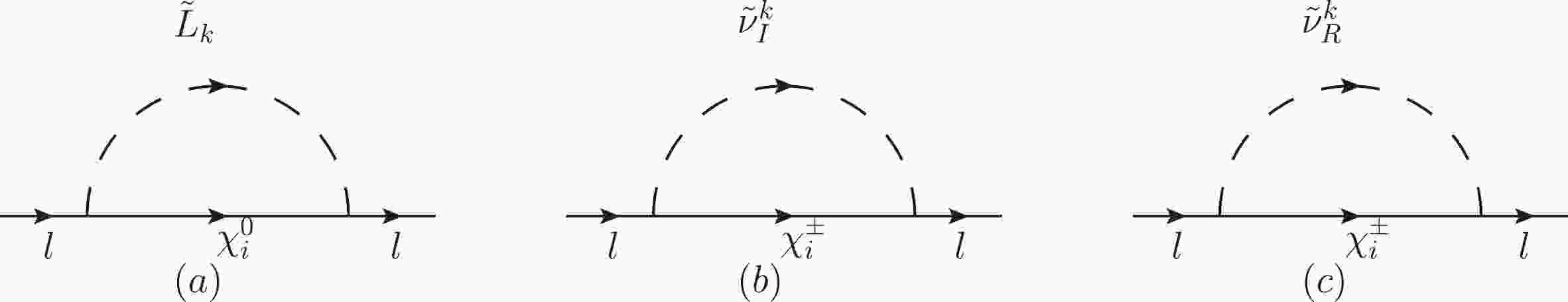
The one-loop new physics contributions to lepton EDMs are taken from the diagrams in Fig. 1. The one-loop contributions to lepton EDMs are obtained via calculation with the on-shell condition of the external lepton. Then, we simplify the analytical results.

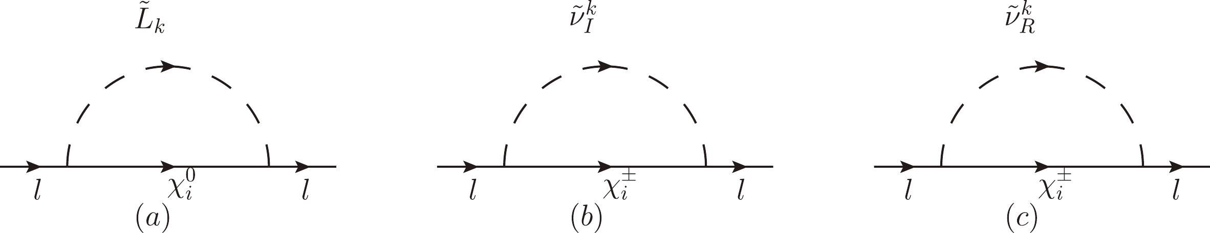
Figure 1.  One-loop self energy diagrams in the $ U(1)_X $SSM.

The analytical results of the one-loop diagrams are shown below.

1. The corrections to lepton EDMs from neutralinos and scalar leptons are

Here, $ x_i=\dfrac{m_i^2}{\Lambda^2} $, where $ m_i $ represents the particle mass, and $ \Lambda $ denotes the new physics energy scale. The couplings $ A_R,A_L $ can be expressed as

The mass matrices of scalar leptons and neutrinos can be diagonalized using the matrices $ Z^{E} $ and $ N $.

The specific forms of the functions $ {\cal{B}}(x,y) $ (using Eq. (11)) and $ {\cal{B}}_1(x,y) $ (using Eqs. (14) and (16)) are

2. The corrections from the chargino and CP-odd scalar neutrino are

The couplings $ B_L $ and $ B_R $ can be expressed as

3. The corrections from the chargino and CP-even scalar neutrino are

The couplings $ C_L $ and $ C_R $ can be expressed as

The $ U $, $ V $, $ Z^{R} $, and $ Z^{I} $ matrices diagonalize the corresponding particle mass matrices, which are detailed in the appendix.

Therefore, the contributions of the one-loop diagrams to lepton EDMs are

In this paper, the two-loop diagrams that we research include the Barr-Zee two-loop diagrams (Fig. 2 (a), (b), (c)) and rainbow two-loop diagrams (Fig. 2 (d), (e)), as shown below.

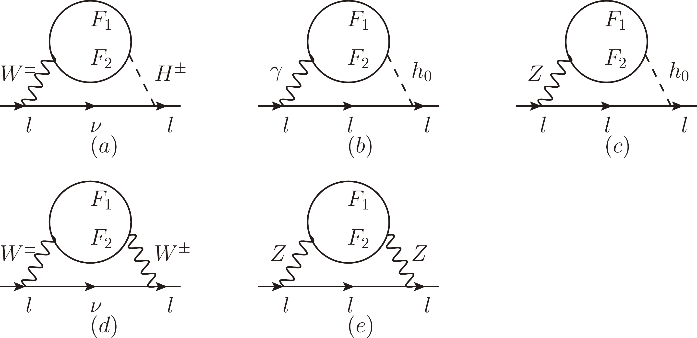
Figure 2.  Two-loop Barr-Zee and rainbow-type diagrams in the $ U(1)_X $SSM.

The analytical results of the contributions from the two-loop diagrams to lepton EDMs are shown below.

The contributions are taken from Fig. 2 (a). Under the assumption that $ m_F=m_{F_1}=m_{F_2}\gg m_W $, the result of simplification [38] is

Here, $ \varrho_{1,1}(x,y)=\dfrac{x\ln x-y\ln y}{x-y} $. $ H_{HF_1F_2}^{L,R} $ and $ H_{WF_1F_2}^{L,R} $ denote the corresponding couplings coefficients. See Ref. [36] for their concrete forms.

Under the assumption that $ m_F=m_{F_1}=m_{F_2}\gg m_{h_0} $, the reduced form of the contribution to the lepton EDM from Fig. 2(b) is

Moreover, the simplified form from Fig. 2(c) is

Here, $ Q_f $ represents the electric charge of the external lepton $ m_\mu $. $ Q_{F_1} $ and $ Q_{F_2} $ denote the electric charges of the internal charginos.

With the assumption that $ m_F=m_{F_1}=m_{F_2}\gg m_W\sim m_Z $, the reduced form of the contribution to the lepton EDM from Fig. 2(d) is

We simplify the tedious two-loop results to the order of $ \dfrac{m_\mu^2}{M_Z^2} \sim 10^{-6} $ or $ \dfrac{m_\mu^2}{m_{\rm SUSY}^2} $ under the assumption that $ m_F = m_{F1} = m_{F2} \gg m_W \sim m_Z $ and obtain the following simplified form of Fig. 2(e):

The contributions to lepton EDMs from the researched two-loop diagrams are

At the two-loop level, the contributions to lepton EDMs can be summarized as

For the numerical discussion, we consider the following experimental limitations. The lightest CP-even higgs mass is considered as an input parameter, which is $ m_{h^0} \approx $ 125.1 GeV [39, 40], and the $ h^0 $ decays are $ h^0 \rightarrow \gamma + \gamma $, $ h^0 \rightarrow Z + Z $, and $ h^0 \rightarrow \gamma + \gamma $ [41]. Experimental constraints on the masses of the new particles are also considered. LHC experiments have more stringent mass constraints on the $ Z^{\prime} $ boson. To satisfy this experimental constraint, we take the parameter $ M_{Z^{\prime}} $ to be greater than 5.1 TeV [42], which is heavier than the previous mass limit. The ratio of $ M_{Z^{\prime}} $ to its gauge coupling $ g_X $ $ (\frac{M_{Z^{\prime}}}{g_X}) $ should not be less than 6 TeV at the $ 99\% $ C.L. [43, 44]. Considering the constraints from the LHC, we set $ \tan{\beta_\eta} < 1.5 $ [45]. Because $ M_{Z^{\prime}} $ has a large mass, the contribution of $ Z^{\prime} $ at the amplitude level is small; therefore, the contribution of $ Z^{\prime} $ is ignored. We adjust the parameters based on the experimental limitation of lepton EDMs. In this section, we research and discuss lepton ($ e, \mu, \tau $) EDMs.

The parameters used in the $ U(1)_X $SSM are

$ \theta_1 $, $ \theta_2 $, and $ \theta_\mu $ are the CP violating phases of the parameters $ m_1 $, $ m_2 $, and $ \mu $. We consider three new CP violating parameters with the phases $ \theta_{BL} $, $ \theta_{BB^{\prime}} $, and $ \theta_S $.

To facilitate the discussion, we make the following simplifications:

Previously, we discussed the EDM of electrons because of its strict experimental upper limit. The CP violating phases $ \theta_1 $, $ \theta_2 $, $ \theta_\mu $, $ \theta_{BL} $, $ \theta_{BB^{\prime}} $, and $ \theta_S $ as well as other parameters have a certain impact on the electron EDM. Now, supposing $ \theta_1 $ = $ \theta_2 $ = $ \theta_\mu $ = $ \theta_{BB^{\prime}} $ = $ \theta_S $ = 0, and setting $ \tan{\beta}=5 $, $ M_2= $ 500 GeV, $ mu= $ 500 GeV, $ M_{BL}= $ 1800 GeV, $ M_{BB^{\prime}}= $ 700 GeV, $ M_S= $ 2400 GeV, $ M_L=$ 1.1 TeV, $ M_E= $ 1.0 TeV. We study the influence of $ \theta_{BL} $on the electron EDM. $ M_{BL} $ is related to the neutralino mass matrix. In Fig. 3, we plot a solid line and dashed line versus $ M_L $ ($ 0.9\sim1.1 \; {\rm TeV^2} $) corresponding to $ M_1 $ = $ 700 $ and 800 GeV. We can see that these two lines are subtractive functions and $ \theta_{BL} $ has an influence on $ |d_e| $. The relationship between $ d_e $ and $ M_L $ is not a simple linear relation; its change curve follows $ M_L^{-2} $. The shaded part of the figure indicates that all these parameters are reasonable and conform to experimental limits.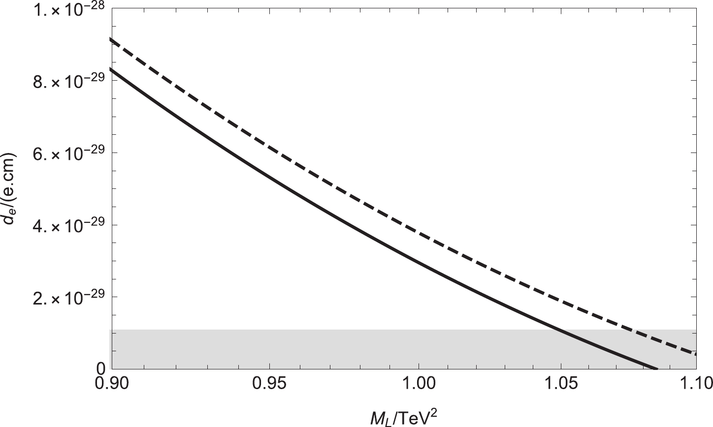

Figure 3.  Setting $ \theta_1 $ = $ \theta_2 $ = $ \theta_\mu $ = $ \theta_{BB^{\prime}} $ = $ \theta_S $ = 0 and $ \theta_{BL} $ = $ \frac{\pi}{4} $, the contributions to the electron EDM varying with $ M_L $ are plotted. The solid and dashed lines correspond to $ M_1 $ = ($ 700,800)\; {\rm GeV} $, respectively.

Setting $ \theta_1 $ = $ \theta_2 $ = $ \theta_\mu $ = $ \theta_{BB^{\prime}} $ = $ \theta_{BL} $ = 0, $ \tan{\beta}=5 $, $ M_1= $ 700 GeV, $ M_2= $ 2000 GeV, $ mu=$ 500 GeV, $ M_{BL}= $ 1600 GeV, $ M_{BB^{\prime}}= $ 800 GeV, $ M_S= -800$ GeV, $ M_{L22}=1.0 $ ${\rm TeV^2} $, and $ M_E=1.0 \; {\rm TeV^2} $, we consider the impact of $ \theta_S $ on the electron EDM. $ M_S $ is related to the mass matrices of the neutralino and scalar lepton. In Fig. 4, $ M_{L11} $ varies from $ 0.5 $ to $ 5.0 \; {\rm TeV^2} $, and when $ M_{L11} > 2.0 \; {\rm TeV^2} $, the numerical results of $ |d_e| $ conform to the experimental limits.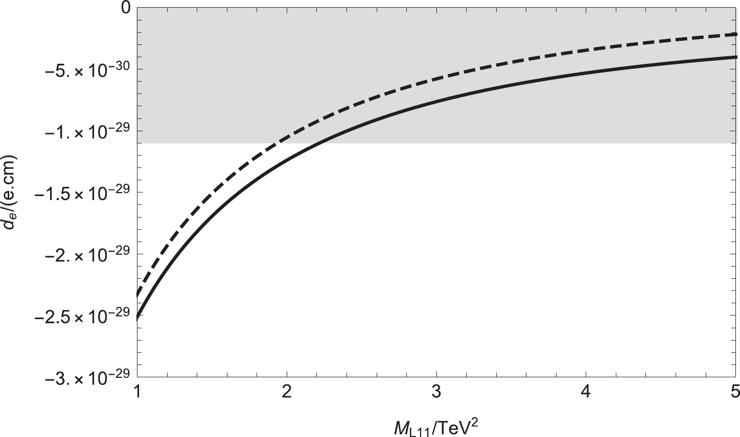

Figure 4.  Setting $ \theta_1 $ = $ \theta_2 $ = $ \theta_\mu $ = $ \theta_{BB^{\prime}} $ = $ \theta_{BL} $ = 0 and $ \theta_S $ = $ \frac{\pi}{4} $, the contributions to the electron EDM varying with $ M_{L11} $ are plotted. The solid and dashed lines correspond to $ M_{L33} $ = $ (1, 0.9)\; {\rm TeV^2} $, respectively.

$ \theta_{BB^{\prime}} $ is the new CP violating phase of the lepton neutrino mass matrix. Therefore, it offers a new physical contribution to the lepton EDM. Setting $ \theta_1 $ = $ \theta_2 $ = $ \theta_\mu $ = $ \theta_S $ = $ \theta_{BL} $ = 0, the contributions to the muon EDM varying with $ T_E $ are plotted, with the solid and dashed lines corresponding to $ M_{E11} $ = 0.5 and 1.0$ \; {\rm TeV^2} $, respectively. Here, we set $ \tan{\beta}=5 $, $ M_1= 700\; {\rm GeV} $, $ M_2=2000\; {\rm GeV} $, $ mu=500\; {\rm GeV} $, $ M_{BL}= $ 1800 GeV, $ M_{BB^{\prime}}= $ 700 GeV, $ M_S= $ 2400 GeV, $ M_L= $ $1.0~{\rm TeV^2} $, and $ M_E=0.5 \; {\rm TeV^2} $. In Fig. 5, the two lines are shaped like parabolas, and most of the numerical results are within the experimental limits.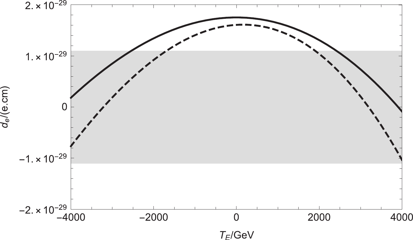

Figure 5.  Setting $ \theta_1 $ = $ \theta_2 $ = $ \theta_\mu $ = $ \theta_S $ = $ \theta_{BL} $ = 0 and $ \theta_{BB^{\prime}} $ = $ \frac{\pi}{3} $, the contributions to the electron EDM varying with $ T_E $ are plotted. The solid and dashed lines correspond to $ M_{E11} $ = $ (0.5,1.0)\; {\rm TeV^2} $, respectively.

We select the parameters $ M_{L11}(0.5\thicksim5.0 \; {\rm TeV^2}) $, $ M_{L22}(0.5\thicksim5.0 \; {\rm TeV^2}) $, $ M_{L33}(0.5\thicksim5.0 \; {\rm TeV^2}) $, $T_E(-3000\thicksim 3000 \; {\rm GeV})$, and $ M_E(0.5\thicksim5.0 \; {\rm TeV^2}) $ and randomly scatter the points. With $ \theta_1 $ = $ \theta_2 $ = $ \theta_\mu $ = $ \theta_{BB^{\prime}} $ = $ \theta_{BL} $ = 0 and $ \theta_S $ = $ \frac{\pi}{4} $, we plot $ |d_e| $ in the plane of $ M_{L11} $ versus $ M_{L22} $ in Fig. 6. "$ \blacksquare $" represents $ |d_e| < 1.1 \times 10^{-29} $ e.cm, and "$ \circ $" represents $ |d_e| \geqslant 1.1 \times 10^{-29} $ e.cm. In Fig. 6, we can see that there is clear stratification. When $ M_{L11} > $ 1.0 $ \; {\rm TeV^2} $, $ M_{L22} $ is in the vicinity of 1.4 $ \; {\rm TeV^2} $, $ |d_e| $ is within the experimental limit. This reveals that $ M_{L11} $ is a sensitive parameter and $ M_{L22} $ is a less sensitive parameter.

Figure 6.  With $ \theta_1 $ = $ \theta_2 $ = $ \theta_\mu $ = $ \theta_{BB^{\prime}} $ = $ \theta_{BL} $ = 0 and $ \theta_S $ = $ \frac{\pi}{4} $, $ |d_e| $ is in the plane of $ M_{L11} $ versus $ M_{L22} $. "$ \blacksquare $" represents $ |d_e| < 1.1 \times 10^{-29} $ e.cm, "$ \circ $" represents $ |d_e| \geqslant 1.1 \times 10^{-29} $ e.cm.

In this section, the muon EDM is numerically studied. In Fig. 7, setting $ \theta_1 $ = $ \theta_\mu $ = $ \theta_{BB^{\prime}} $ = $ \theta_2 $ = $ \theta_{BL} $ = 0 and $ \tan{\beta}=6 $, $ M_1= $ 1450 GeV, $ M_2=$ 2000 GeV, $ mu=$ 500 GeV, $ M_{BB^{\prime}}= $ 800 GeV, $ M_S= -800$ GeV, $ M_L=1.0 $ $ {\rm TeV^2} $, and $ M_E=0.5 \; {\rm TeV^2} $. We study the influence of $ \theta_S $ on the muon EDM. The solid and dashed lines correspond to $ M_{BL} $ ($ 1200 $, 1500 GeV), respectively. From the numerical results, we can see that the muon EDM increases as $ M_E $ increases. $ \theta_S $ has a significant influence on the numerical results because $ M_S $ is related to the mass matrices of the neutralino and charged Higgs.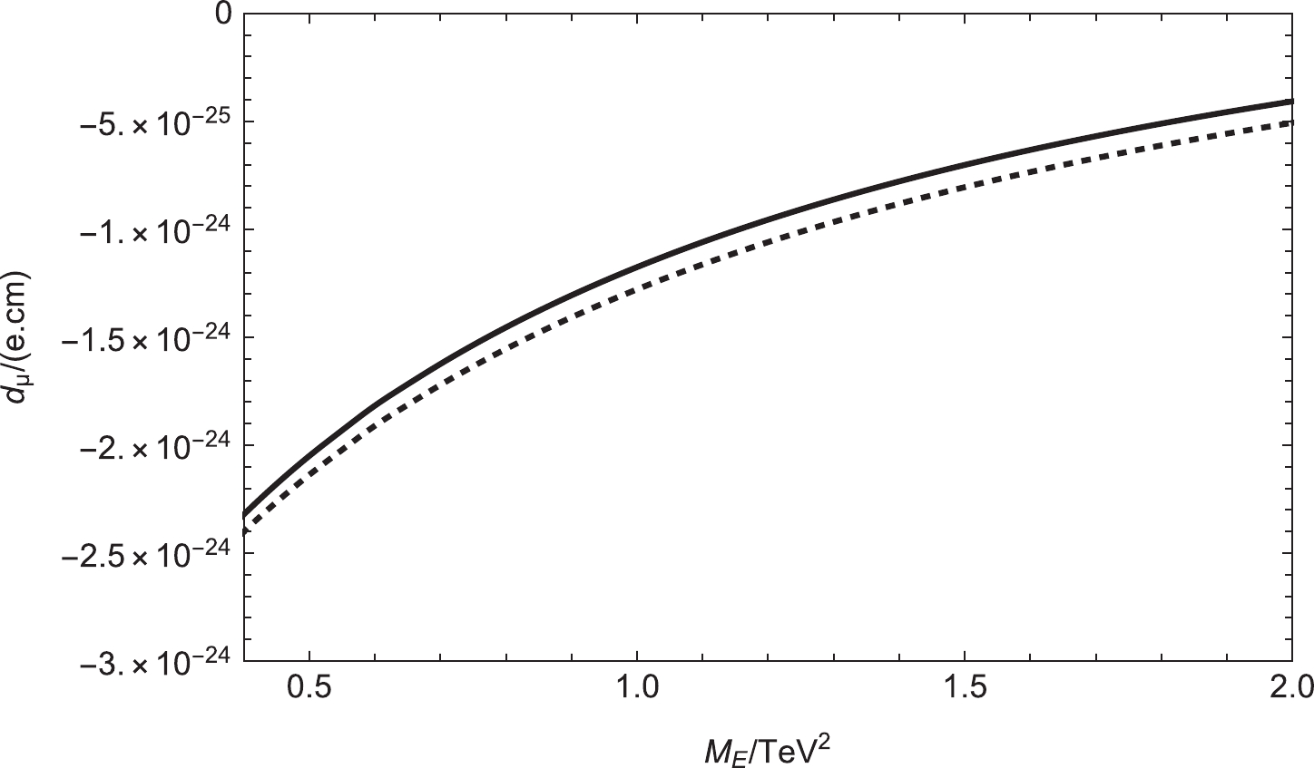

Figure 7.  Setting $ \theta_1 $ = $ \theta_2 $ = $ \theta_\mu $ = $ \theta_{BB^{\prime}} $ = $ \theta_{BL} $ = 0 and $ \theta_S $ = $ \frac{\pi}{3} $, the contributions to the muon EDM varying with $ M_E $ are plotted. The solid and dashed lines correspond to $ M_{BL} $ = $ (1200,1500)\; {\rm GeV} $.

$ \theta_{BB^{\prime}} $ is the new CP violating phase of the neutralino mass matrix. Therefore, it offers a new physical contribution to the lepton EDMs. With $ \theta_1 $ = $ \theta_2 $ = $ \theta_\mu $ = $ \theta_S $ = $ \theta_{BL} $ = 0, the contributions to the muon EDM varying with $ M_{E22} $ are plotted, where the solid and dashed lines correspond to $ \tan\beta $ = (5, 6), respectively. In this part, we set $ M_1= $ 1450 GeV, $ M_2= $ 800 GeV, $ mu= $ 500 GeV, $ M_{BL}= $ 1600 GeV, $ M_{BB^{\prime}}= $ 800 GeV, $ M_S= -800$ GeV, $ M_L=1.0 \; {\rm TeV^2} $, and $ M_E=0.5 \; {\rm TeV^2} $. In Fig. 8, as $ M_{E22} $ increases, the numerical results gradually decrease, and the shapes of the two lines are similar.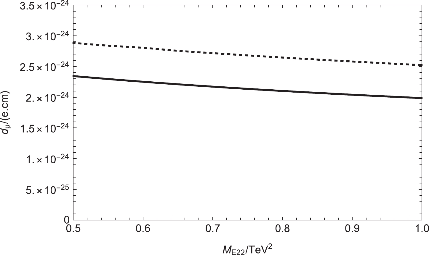

Figure 8.  Setting $ \theta_1 $ = $ \theta_2 $ = $ \theta_\mu $ = $ \theta_S $ = $ \theta_{BL} $ = 0 and $ \theta_{BB^{\prime}} $ = $ \frac{\pi}{6} $, the contributions to the muon EDM varying with $ M_{E22} $ are plotted. The solid and dashed lines correspond to $ \tan\beta $ = ($ 5,6 $).

We choose the parameters $ M_{L11}(0.5\thicksim5.0 \; {\rm TeV^2}) $, $ M_{L22}(0.5\thicksim5.0 \; {\rm TeV^2}) $, $ M_{L33}(0.5\thicksim5.0 \; {\rm TeV^2}) $, $T_E(-3000\thicksim 3000 \; {\rm GeV})$, and$ M_E(0.5\thicksim5.0 \; {\rm TeV^2}) $ and randomly scatter the points. With $ \theta_1 $ = $ \theta_2 $ = $ \theta_\mu $ = $ \theta_{BB^{\prime}} $ = $ \theta_{BL} $ = 0, and $ \theta_S $ = $ \frac{\pi}{4} $, we study $ |d_\mu| $ in the plane of $ M_{L33} $ versus $ M_E $. In Fig. 9, "$ \blacksquare $" represents $ |d_\mu| < 1\times10^{-24} $ e.cm, and "$ \circ $" represents $ |d_\mu| \geqslant 1\times10^{-24} $ e.cm. Delamination occurs when $ M_E $ = $ 1.1 \; {\rm TeV^2} $, and stratification is clear. This reveals that $ M_{E} $ is a sensitive parameter and $ M_{L33} $ is an insensitive parameter. These parameters are in a reasonable parameter space.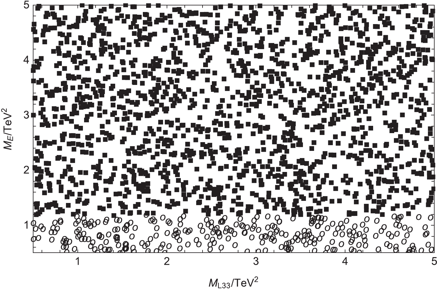

Figure 9.  With $ \theta_1 $ = $ \theta_2 $ = $ \theta_\mu $ = $ \theta_{BB^{\prime}} $ = $ \theta_{BL} $ = 0 and $ \theta_S $ = $ \frac{\pi}{4} $, $ |d_{\mu}| $ is in the plane of $ M_{L33} $ versus $ M_{E} $, where "$ \blacksquare $" represents $ |d_\mu| < 1\times10^{-24} $ e.cm, and "$ \circ $" represents $ |d_\mu| \geqslant 1\times10^{-24} $ e.cm.

At present, the experimental upper bound of the tau EDM is $ |d^{\rm exp}_{\tau}| < 1.1 \times 10^{-17} $ e.cm, which is largest among the bounds of lepton EDMs. Therefore, we now study the tau EDM. With $ \tan{\beta}=6 $, $ M_1= $ 750 GeV, $ mu= $ 650 GeV, $ M_{BL}= $ 1800 GeV, $ M_{BB^{\prime}}= $ 700 GeV, $ M_S= $ 1400 GeV, $ M_L=1.0 \; {\rm TeV^2} $, and $ M_E=1.0 \; {\rm TeV^2} $ and setting $ \theta_1 $ = $ \theta_2 $ = $ \theta_\mu $ = $ \theta_{BB^{\prime}} $ = $ \theta_{BL} $ = 0 and $ \theta_S $ = $ \frac{\pi}{5} $, we study the influence of $ M_{L33} $ on $ |d_\tau| $. In Fig. 10, the solid and dashed lines correspond to $ M_2 $ = $ (400 $, 500 GeV), respectively, and their numerical results are all in the negative. The two lines are increasing functions of $ M_{L33} $, and $ \theta_S $ has clearer influence on the numerical result of $ |d_{\tau}| $. The maximum value of the two lines reaches $ 5.0 \times 10^{-23} $ e.cm, and this value is six orders of magnitude smaller than the upper limit of the experiment.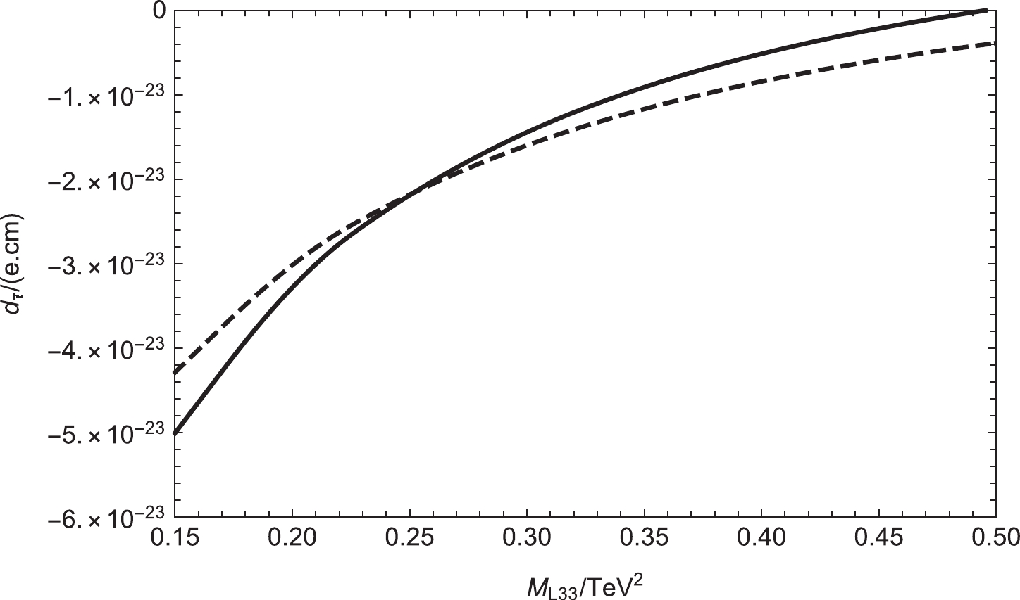

Figure 10.  Setting $ \theta_1 $ = $ \theta_2 $ = $ \theta_\mu $ = $ \theta_{BB^{\prime}} $ = $ \theta_{BL} $ = 0 and $ \theta_S $ = $ \frac{\pi}{5} $, the contributions to the tau EDM varying with $ M_{L33} $ are plotted. The solid and dashed lines correspond to $ M_2 $ = $ (400,500)\; {\rm GeV} $, respectively.

$ \theta_{BL} $ is the new CP violating phase of $ M_{BL} $ in the neutralino mass matrix. Setting $ \tan{\beta}=6 $, $ M_1= $ 750 GeV, $ M_2= $ 400 GeV, $ M_{BL}= $ 1800 GeV, $ M_{BB^{\prime}}= $ 700 GeV, $ M_S= $ 1400 GeV, $ M_E=1.0 \; {\rm TeV^2} $, $ \theta_1 $ = $ \theta_2 $ = $ \theta_\mu $ = $ \theta_{BB^{\prime}} $ = $ \theta_S $ = 0, and $ \theta_{BL} $ = $ \frac{\pi}{6} $, the contributions to the tau EDM varying with $ M_L $ are plotted, where the solid and dashed lines correspond to $ mu $ = $ (650,750 \; {\rm GeV} $), respectively. In Fig. 11, we can see that $ |d_\tau| $ decreases with increasing $ M_L $. The maximum value of these two lines reaches $ |d_\tau| $ = $ 4.5 \times 10^{-23} $ e.cm.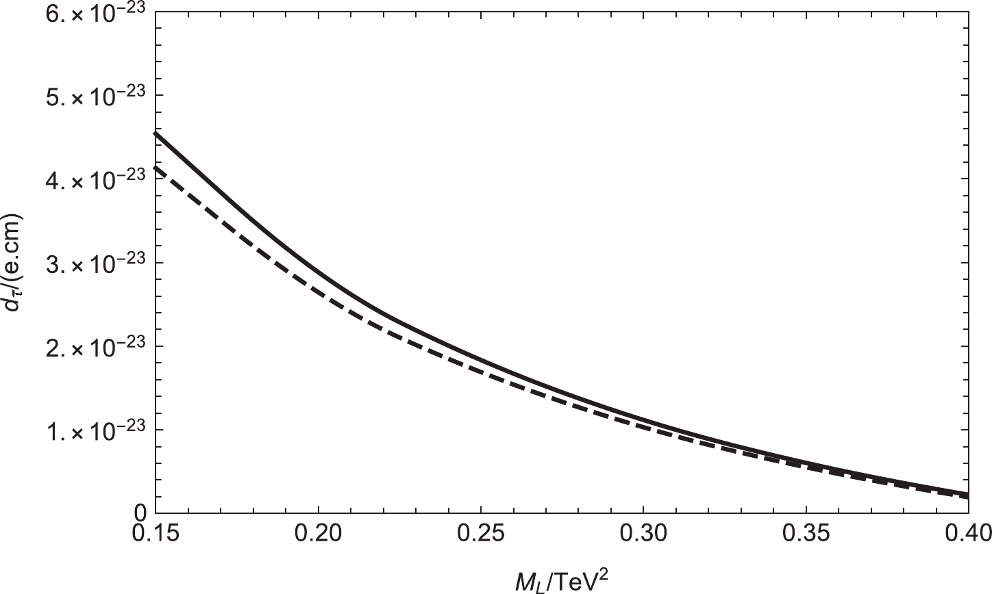

Figure 11.  Setting $ \theta_1 $ = $ \theta_2 $ = $ \theta_\mu $ = $ \theta_S $ = $ \theta_{BB^{\prime}} $ = 0 and $ \theta_{BL} $ = $ \frac{\pi}{6} $, the contributions to the tau EDM varying with $ M_L $ are plotted. The solid and dashed lines correspond to $ mu $ = $ (650,750)\; {\rm GeV} $.

We select the parameters $ M_{L11}(0.5\thicksim5.0 \; {\rm TeV^2}) $, $ M_{L22}(0.5\thicksim5.0 \; {\rm TeV^2}) $, $ M_{L33}(0.5\thicksim5.0 \; {\rm TeV^2}) $, $ T_E(-3000\thicksim 3000 \; {\rm GeV}) $, and $ \tan{\beta}(2\thicksim20) $ and randomly scatter the points. In Fig. 12, we study $ |d_\tau| $ in the plane of $ M_{L33} $ and $ \tan{\beta} $ to observe their influence. The varying regions of $ M_{L33} $ and $ \tan{\beta} $ are in the range $ (0.5\thicksim5 \; \rm TeV^2) $ and $ (2\thicksim20) $, respectively."$ \blacksquare $" represents $ |d_\tau| < 1 \times 10^{-23} $ e.cm, and "$ \circ $" represents $|d_\tau| \geqslant 1 \times 10^{-23}$ e.cm. When $ \tan{\beta} $ = 6, stratification occurs, and the stratification is more clear. This indicates that $ \tan{\beta} $ is a sensitive parameter.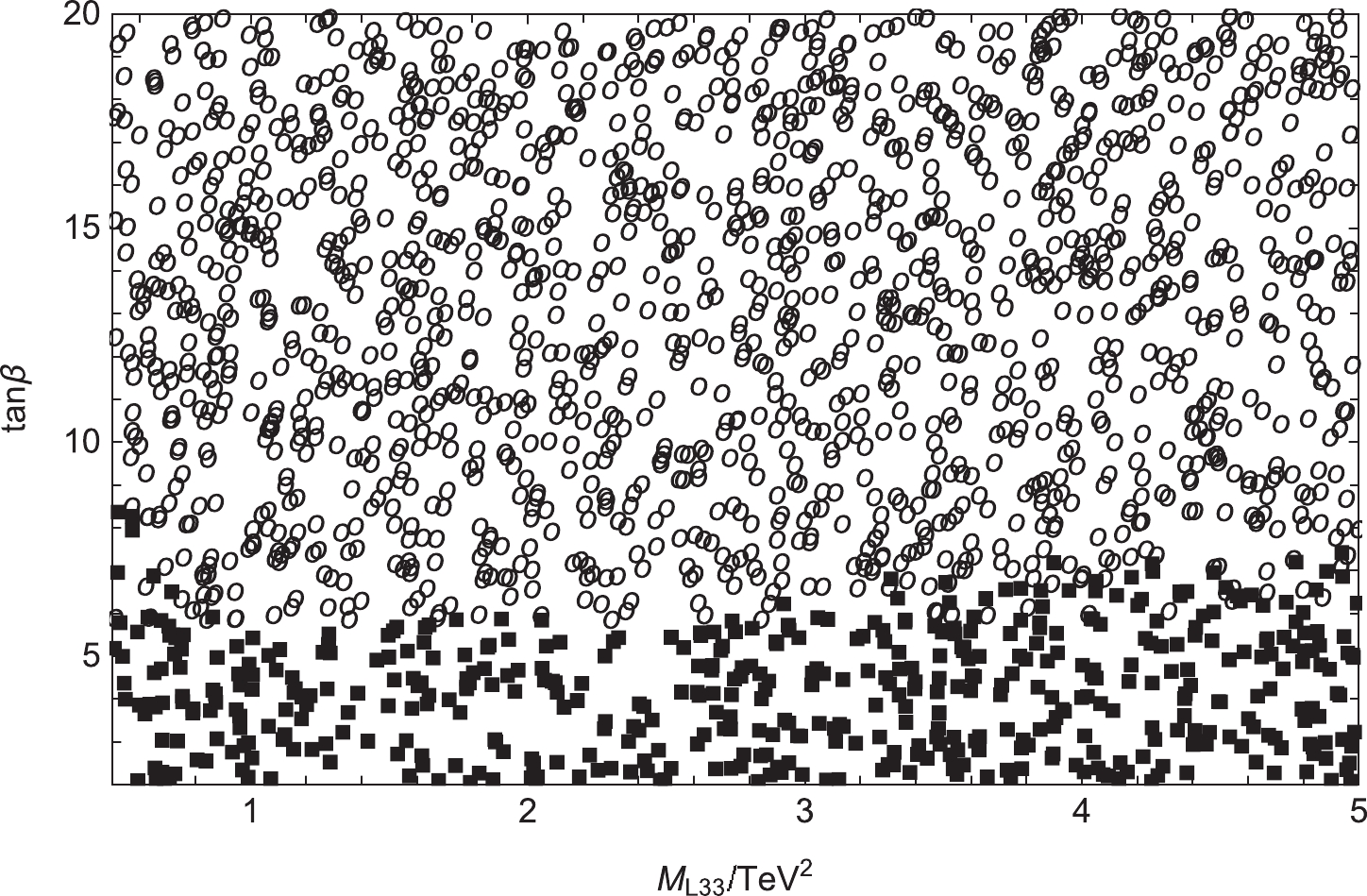

Figure 12.  With $ \theta_1 $ = $ \theta_2 $ = $ \theta_\mu $ = $ \theta_{BB^{\prime}} $ = $ \theta_S $ = 0 and $ \theta_{BL} $ = $ \frac{\pi}{6} $, $ |d_{\tau}| $ is in the plane of $ M_{L33} $ versus $ \tan{\beta} $. "$ \blacksquare $" represents $ |d_\tau| < 1 \times 10^{-23} $ e.cm, and "$ \circ $" represents $ |d_\tau| \geqslant 1 \times 10^{-23} $ e.cm.

In the $ U(1)_X $SSM, we calculate and analyze one-loop and two-loop contributions to lepton ($ e,\mu,\tau $) EDMs. The effects of the CP violating phases $ \theta_1 $, $ \theta_2 $, $ \theta_\mu $, $ \theta_{BB^{\prime}} $, $ \theta_S $, and $ \theta_{BL} $ on the lepton EDMs are researched. Among them, $ \theta_{BB^{\prime}} $, $ \theta_S $, and $ \theta_{BL} $ are all newly introduced. The experimental upper limit of the electron EDM is $|d^{\rm exp}_e| < 1.1 \times 10^{-29}$ e.cm, which places strict restrictions on the $ U(1)_X $SSM parameter space. In the parameter space used in this study, the numerical result for $ |d_e| $ can be controlled below the experimental limit. In our study, the largest numerical results for the $ \mu $ EDM and $ \tau $ EDM are approximately $ 2.8 \times 10^{-24} $ e.cm and $ 5.0 \times 10^{-23} $ e.cm, respectively. They are all in a reasonable parameter space and do not exceed the upper limit of the experiment. For the corrections of the lepton EDMs, the one-loop contributions are dominant. As for the one-loop and two-loop contributions to the EDMs, their relative size $(d_l^{\rm two-loop} /d_l^{\rm one-loop})$ is approximately $ 5\%\thicksim15\% $ after numerical calculation.

Our numerical results mainly obey the rule $ d_e / d_\mu / d_\tau \thicksim m_e / m_\mu / m_\tau $. In Fig. 3, when $ \theta_{BL} $ = $ \frac{\pi}{4} $, $ M_L $ has a more obvious impact on the electron EDM, and the influence of $ \theta_{BL} $ on the electron EDM is also more obvious. In addition, the influences of the CP-violating phases $ \theta_{S} $ and $ \theta_{BB^{\prime}} $ on lepton EDMs are clear. In Fig. 7, when $ \theta_{S} $ = $ \frac{\pi}{3} $, the value of the muon EDM increases as $ M_E $ increases (the numerical results are all negative). $ \theta_{S} $ has a significant influence on the numerical results because $ M_S $ is related to the mass matrices of the neutralino and charged Higgs. In Fig. 8, when $ \theta_{BB^{\prime}} $ = $ \frac{\pi}{6} $, the two lines (solid and dashed lines) are decreasing functions of $ M_{E22} $. The above parameters ($ M_L $, $ M_E $) are all elements on the diagonal of the mass matrix; therefore, their corresponding results are all decoupled, such as in Fig. 3, Fig. 4, Fig. 7, Fig. 8, Fig. 10, and Fig. 11. In Fig. 12, We can see that $ |d_\tau| $ increases with increasing $ \tan\beta $. If we use the method of mass insertion [46] to analyze the results, we can intuitively find that $ \tan\beta $ is proportional to lepton EDMs. We also perform random spot operations on lepton EDMs. The randomly scattered pictures exhibit clear stratification, which also helps us find a reasonable parameter space. As the accuracy of technology improves in the near future, lepton EDMs may be detected.

The mass matrix for a slepton with the basis $ (\tilde{e}_L,\tilde{e}_R) $

This matrix is diagonalized by $ Z^E $

The mass matrix for a CP-even sneutrino $ ({\phi}_{l}, {\phi}_{r}) $ reads as

This matrix is diagonalized by $ Z^R $

The mass matrix for a CP-odd sneutrino $ ({\sigma}_{l}, {\sigma}_{r}) $ is deduced as

This matrix is diagonalized by $ Z^I $

The mass matrix for charginos in the basis ($ \tilde{W}^- $,$ \tilde{H}_d^- $),($ \tilde{W}^+ $,$ \tilde{H}_u^+ $)

The matrix is diagonalized by U and V

The mass matrix for charged Higgs in the basis ($ H_d^{-} $,$ H_u^{+,*} $),($ H_d^{-,*} $,$ H_u^{+} $)

This matrix is diagonalized by $ Z^+ $

The mass matrix for a neutralino in the basis ($ \lambda_{\tilde{B}} $,$ \tilde{W}^0 $,$ \tilde{H}_d^0 $,$ \tilde{H}_u^0 $,$ \lambda_{\tilde{X}} $,$ \tilde{\eta} $,$ \tilde{\bar{\eta}} $,$ \tilde{s} $) is

This matrix is diagonalized by $ N $,