


 Abstract
 HTML
HTML Reference
 Related
 PDF
PDF


-
An accurate description of the synthesis of heavy elements in the Universe is a prominent topic open to investigation in the field of nuclear astrophysics, and the type of particles involved in nuclear processes is among the foundations of this investigation [1, 2]. Although the majority of heavy elements are produced via two neutron-induced processes, known as slow (s) and rapid (r) processes [3, 4], there are 35 neutron-deficient stable nuclei (from 74Se to 196Hg), the so-called p nuclei, that cannot be created in these scenarios. These are related to the p-process (or γ-process) with photodisintegration reactions of (γ, n), (γ, p), and (γ, α) [5]. With the exception of nucleosynthesis in nature, there are roughly 7000 possible candidates in the nuclear landscape. However, to date, only roughly 3000 nuclides have been identified, and the vast territory remains to be explored [6−8]. The location of the dripline, defined unambiguously by the nucleon or two-nucleon separation energies [9], depicts the boundary of the nuclear landscape, which is essential for understanding the relationships between the total number of nuclides and the nuclear force [10].
The masses and half-lives of nuclei are important inputs in nuclear astrophysics; therefore, accurate measurements for nuclei are of significant importance. Unfortunately, the measurement of unknown nuclear masses is not always feasible, even with the latest experimental technology. Experimentally, only the neutron dripline of nuclides with
$ Z\leqslant10 $ have been determined [11]. Thus, theoretical models become crucial for evaluating and predicting unknown masses.Various mass models have been proposed and corrected in the last several decades. Myers and Swiatecki developed the semi-empirical droplet model of nuclear masses and deformations [12, 13]. The finite-range droplet model, which was developed from a Yukawa-plus-exponential macroscopic model (finite-range liquid-drop model) and a folded-Yukawa single-particle potential for microscopic energy, was proposed by Möller et al. in 1981 and corrected in the following years [14−19]. In addition, Hartree-Fock-Bogoliubov theory has been applied to the determination of nuclear masses, and numerous versions have been developed using the Skyrme-type and Gogny-type effective interactions [20−22]. Furthermore, time-dependent Hartree-Fock has been used to describe multinucleon transfer dynamics [23].
In this paper, we conduct a shell-model study on the proton dripline properties of nuclides with
$ Z, N=30-50 $ , which are of importance in astrophysical νp-processes. In addition, several nuclei are important in Type I X-ray bursts [24, 25]. A full$ f_{5}pg_{9} $ shell model calculation is applied to investigate the binding energies, proton separation energies, and proton dripline properties (including the partial half-lives of proton emission) of these exotic nuclei. The formulas for energy calculation are introduced in Sec. II.A. Furthermore, the confidence of our results is also examined with an uncertainty decomposition framework [28] based on the bootstrap method [29, 30]; this framework is presented in Sec. II.B. Finally, the results are discussed in Sec. III. -
In recent years, several properties of light proton-rich nuclei have been studied via experiments, and the shell model has provided reasonable theoretical descriptions of, e.g., isospin asymmetry [31, 32], β-delayed proton(s) emission [33, 34], β-decay spectroscopy [35, 36], the exotic β-γ-α decay mode of 20Na [37], and the four-proton unbound nucleus 18Mg [38]. In neutron-deficient heavy nuclei, the shell model effectively describes the α-decay of the lightest isotope of U [39] and isomeric states of 218Pa [40] and 213Th [41]. For medium mass nuclei, investigations are located mostly in neutron-rich nuclei [42−44] and neutron-deficient nuclei with
$ Z\leqslant N $ [45−47]; this rarely exceeds$ Z=N $ .The shell model provides many descriptions of nuclear spectroscopic properties but rarely investigates the binding energy. A reasonable choice of effective interaction is key to performing shell-model calculations. Through the interaction, shell-model calculations provide the valence part of the binding energy without considering the Coulomb interaction. This is noted as
$ E_{\rm BE, SM}(Z, N) $ , where$ Z (N) $ denotes the proton (neutron) number. The effective interaction JUN45, which was proposed by Honma et al. via fitting to the experimental data of selected nuclides in the$ f_{5}pg_{9} $ shell model space consisting of four single-particle orbits$ p_{3/2} $ ,$ f_{5/2} $ ,$ p_{1/2} $ , and$ g_{9/2} $ [48], is used in the present study to calculate$ E_{\rm BE,SM}(Z,N) $ . To estimate the binding energy based on the shell model, several corrections should be considered. In 1997, Herndl and Brown [49] used an overall constant ($ cst $ ) and four terms, linear and quadratic, for the number of valence protons and neutrons:$ \begin{aligned}[b] E_{\rm BE}(Z,N)=&E_{\rm BE,SM}(Z,N)+cst+a(Z-28)\\ &+b(Z-28)^2+c(N-28)^2+d(N-28), \end{aligned} $

(1) where a, b, c, and d are fitting parameters. This form is equivalent to the combination of the two body Coulomb interaction and a small variation in the nuclear size and mass [49].
Analogous of Eq. (1), one can construct a quadratic formula for the binding energy of a certain nuclide by fixing the constant term of the original formula with the binding energy of 56Ni:
$ \begin{aligned}[b] E_{\rm BE}(Z,N)=&E_{\rm BE, SM}(Z, N) + E_{\rm BE}(^{56}{\rm{Ni}}) + a(Z-28)\\& + b(Z-28)^{2} + c(N-28)^{2} + d(N-28). \end{aligned} $

(2) The correction for the Coulomb energy is included in the a and b terms. In addition, the single-particle energies of the core, which remain unchanged for all nuclides, may actually depend on the number of valence nucleons and should be compensated for by introducing additional terms to Z and N, as suggested in Eq. (2). Through the fitting results, we suggest replacing the last term of Eq. (2) with the difference between valence protons and neutrons:
$ \begin{aligned}[b] E_{\rm BE}(Z,N)=&E_{\rm BE, SM}(Z,N) + E_{\rm BE}(^{56}{\rm{Ni}}) + a(Z-28) \\&+ b(Z-28)^{2} + c(N-28)^{2} + d(Z-N)^{2}. \end{aligned} $

(3) Moreover, the sum of the last two terms and the residuals of Eqs. (2) and (3) reveals a hyperboloid-like distribution. Thus, it is approached with the term
$ (Z-30)(Z- 2N+50) $ :$ \begin{aligned}[b] E_{\rm BE}(Z,N)=&E_{\rm BE, SM}(Z,N) + E_{\rm BE}(^{56}{\rm{Ni}}) + a(Z-28) \\&+ b(Z-28)^{2} + c(Z-30)(Z-2N+50). \end{aligned} $

(4) Furthermore, Caurier
$ et \ al. $ [50] proposed a correction including a modified Coulomb energy term and a monopole expression:$ \begin{array}{*{20}{l}} E_{\rm BE}(Z,N)=E_{\rm BE, SM}(Z,N) + E_{\rm BE}(^{56}{\rm{Ni}}) + E_{\rm C} + E_{\rm M}, \end{array} $

(5) with
$ \begin{aligned}[b] E_{\rm C} =& a(Z-28) + b(Z-28)(Z-29) + c(Z-28)(N-28), \\ E_{\rm M} =& d(A-56) + e(A-56)(A-57) + f(T(T+1)-\frac{3}{4}(A-56)), \end{aligned} $

where T is the isospin of the nuclide, and A is the mass number. It is found that Eqs. (3) and (5) are relatively similar. The difference between them is a term involving the gap of the total isospin. When focusing on the ground state property, a general rule is that
$ T \approx T_{3} \propto |N-Z| $ . Thus, the term involving the isospin could also be absorbed in the quadratic form of nucleon numbers.Nucleon separation energies can be easily calculated via the binding energy using the following formulas:
$ S_{p}(Z, N)= E_{\rm BE}(Z,N)-E_{\rm BE}(Z-1,N) $ and$ S_{2p}(Z, N)= E_{\rm BE}(Z,N)- E_{\rm BE}(Z-2,N) $ . From Eqs. (3) and (4), the general forms of$ S_ {p} $ and$ S_ {2p} $ are deduced as$ \begin{aligned}[b] S_{ p}(Z, N) =& E_{\rm BE, SM}(Z, N) - E_{\rm BE, SM}(Z-1, N) \\ & + aZ + bN + d, \end{aligned} $

(6) $ \begin{aligned}[b] S_{ 2p}(Z, N) =& E_{\rm BE, SM}(Z, N) - E_{\rm BE, SM}(Z-2, N) \\ & + aZ + bN + d. \end{aligned} $

(7) Although the quadratic term,
$ c(Z-N)^{2} $ , disappears by subtracting the two binding energies, it exhibits a correlation with the residuals of Eqs. (6) and (7). After reintroducing this term,$ \begin{aligned}[b] S_{ p}(Z, N)=&E_{\rm BE, SM}(Z, N) - E_{\rm BE, SM}(Z-1, N) \\ & + aZ + bN + c(Z-N)^{2} + d, \end{aligned} $

(8) $ \begin{aligned}[b] S_{ 2p}(Z, N)=&E_{\rm BE, SM}(Z, N) - E_{\rm BE, SM}(Z-2, N) \\ & + aZ + bN + c(Z-N)^{2} + d, \end{aligned} $

(9) perform well to describe the experimental data with lower uncertainties, as listed in Table 1. Furthermore, the value (uncertainty) of the fitting parameter b significantly decreases (increases) after the reintroduction of
$ c(Z-N)^{2} $ , which reveals the redundancy and unreliability of b. The term$ bN $ is no more robust in Eqs. (8) and (9) and will increase the statistical uncertainty of the formulas. As expected, removing this term makes the following formulas perform better:$\sigma_{\rm total}$ *

$\sigma_{\rm stat}$ *

$ \sigma_{\rm sys} $ *

$ \sigma_{\rm total} $ #

$ \sigma_{\rm stat} $ #

a b c d e f $ E_{\rm BE}\rm (Eq. (2)) $ 

0.731 0.122 0.721 0.774 0.281 −9.15 (5) −0.0954 (25) 0.0188 (12) −0.276 (31) — — $ E_{\rm BE}\rm (Eq. (3)) $ 

0.316 0.0482 0.312 0.416 0.275 −9.61 (1) −0.0944 (8) 0.0245 (5) −0.0262 (9) — — $ E_{\rm BE}\rm (Eq. (4)) $ 

0.317 0.0399 0.315 0.374 0.202 −9.12 (1) −0.0921 (7) −0.0309 (5) — — — $ E_{\rm BE}\rm (Eq. (5)) $ 

0.305 0.0563 0.300 0.779 0.719 −9.45 (8) −0.118 (1) 0.425 (98) 0.0221 (158) −0.0939 (244) 0.363 (96) $ S_{ p}\rm (Eq. (6)) $ 

0.286 0.0362 0.284 0.294 0.0781 −0.242 (6) 0.0548 (52) — −4.28 (19) — — $ S_{ p}\rm (Eq. (8)) $ 

0.276 0.0404 0.273 0.375 0.257 −0.186 (16) 0.00385 (1541) 0.00335 (88) −4.36 (19) — — $ S_{ p}\rm (Eq. (10)) $ 

0.275 0.0331 0.273 0.278 0.0519 −0.182 (5) — 0.00359 (27) −4.36 (19) — — $ S_{ p}\rm (Eq. (22)) $ 

0.231 0.0328 0.228 0.233 0.0447 −0.183 (4) — 0.00364 (25) −4.14 (16) −0.302 (33) — $ S_ {2p}\rm (Eq. (7)) $ 

0.306 0.0449 0.303 0.320 0.102 −0.478 (8) 0.105 (7) — −8.36 (22) — — $ S_{ 2p}\rm (Eq. {9}) $ 

0.265 0.0439 0.261 0.390 0.289 −0.360 (19) −0.00125 (1794) 0.00736 (111) −8.55 (21) — — $ S_{ 2p}\rm (Eq. (11)) $ 

0.264 0.0355 0.261 0.267 0.0527 −0.361 (5) — 0.00729 (34) −8.55 (20) — — * Calculated uncertainties for these nuclides with experimentally known data.
# Calculated uncertainties for these nuclides without experimentally known data.Table 1. Fitting parameters, decomposed uncertainties for experimentally determined nuclides, and recomposed uncertainties for the extrapolation of the binding energy,
$ S_ {p} $ and$ S_ {2p} $ formulas with standard deviation. The unit is MeV.$ \begin{array}{*{20}{l}} S_{ p}(Z, N)=&E_{\rm BE, SM}(Z, N) - E_{\rm BE, SM}(Z-1, N) \\ & + aZ + c(Z-N)^{2} + d, \end{array} $

(10) $ \begin{array}{*{20}{l}} S_{ 2p}(Z, N)= &E_{\rm BE, SM}(Z, N) - E_{\rm BE, SM}(Z-2, N) \\ & + aZ + c(Z-N)^{2} + d. \end{array} $

(11) The performance of these formulas for the binding and separation energies is investigated via application of the bootstrap method, which is introduced in the subsequent section.
-
The total uncertainty of a formula is composed of the experimental, statistical, and systematic uncertainties [26, 27]. Our previous study [28] detailed the practical steps of the bootstrap method [29, 30] for decomposing and recomposing uncertainties. Recently, Jia et al. used this to study the correlation between the parameters of the Woods-Saxon potential and evaluate the uncertainty of the binary cluster model [51]. The benefit of such a method is that all useful statistics can be obtained simultaneously from the parameter space estimated from the resampling of the dataset. Note that the experimental uncertainties of binding and separation energies are neglected here because they are generally (more than 95%) smaller than 0.1 MeV. The residual between the theoretical and experimental data of a nuclide with Z protons and N neutrons is defined as
$ \begin{array}{*{20}{l}} r(Z, N, S_{ {\rm BS}, i}) = y_{\rm cal}(Z, N, S_{ {\rm BS}, i})-y_{\rm exp}(Z, N), \end{array} $

(12) where y denotes the corresponding energy, the subscript
$ {\rm cal} $ denotes the calculated value, the subscript$ {\rm exp} $ denotes the experimental value, and$ S_ {{\rm BS}, i} $ denotes the ith bootstrap sample among the M bootstrap samples, which are of the same sizes as those in the original dataset. In practice, the number of bootstrap samples is set to be$ M = 10^6 $ , which assures a robust estimation of uncertainties. The ordinary least squares method is used to perform the fitting. Under this definition, a positive value of$ r(Z, N, S_ {{\rm BS}, i} $ ) indicates an overestimation, whereas a negative value indicates an underestimation. The statistical uncertainty of a formula for a nuclide is defined by the unbiased standard deviation$ \begin{array}{*{20}{l}} \hat{\sigma}_{\rm stat}^{2}\left(Z, N\right)=\dfrac{1}{M-1} \displaystyle\sum\limits_{i=1}^{M}\left(y_{\rm cal}\left(Z, N, S_{ {\rm BS}, i}\right) - \bar{y}_{\rm cal}\left(Z, N\right)\right)^{2}, \end{array} $

(13) where
$ \bar{y}_{\rm cal}(Z, N) $ is the mean of the calculated values for a given nuclide. The global statistical uncertainty of a formula is the root-mean-square (rms) of$ \hat{\sigma}_{\operatorname{\rm stat}}\left(Z, N\right) $ :$ \begin{array}{*{20}{l}} \hat{\sigma}_{\rm stat}^{2}=\dfrac{1}{K} \displaystyle\sum\limits_{k=1}^{K} \hat{\sigma}^{2}_{\rm stat}\left(Z, N\right), \end{array} $

(14) where K is the number of combinations of protons and neutrons in the dataset.
By ignoring the experimental uncertainty, the systematic uncertainty, which yields the gaps between the calculated and "true" values, is estimated by
$ \begin{aligned}[b] \hat{\sigma}^{2}_{\rm sys}\left(Z, N\right)&=\left(\displaystyle\sum\limits_{i=1}^{M} \frac{y_{\rm cal}\left(Z, N, S_{ {\rm BS}, i}\right)}{M} - y_{\rm exp}\left(Z, N\right)\right) ^{2} \\ &= \left( \frac{1}{M} \displaystyle\sum\limits_{i=1}^{M} r\left(Z, N, S_{ {\rm BS}, i}\right) \right)^{2}, \end{aligned} $

(15) and the global systematic uncertainty is derived using
$ \hat{\sigma}_{\rm sys}^{2}=\dfrac{1}{K} \displaystyle\sum\limits_{k=1}^{K} \hat{\sigma}^{2}_{\rm sys}\left(Z, N\right) = \dfrac{1}{K} \displaystyle\sum\limits_{k=1}^{K} \bar{r}^{2}\left(Z, N\right). $

(16) The total uncertainty of a property for a nuclide is defined by the rms of the residuals
$ \begin{aligned}[b] \hat{\sigma}_{\rm total}^{2}\left(Z, N\right) & =\frac{1}{M} \sum\limits_{i=1}^{M} r^{2}\left(Z, N, S_{ {\rm BS}, i}\right) \\ & =\frac{M-1}{M} \hat{\sigma}_{\rm stat}^{2}\left(Z, N\right)+\hat{\sigma}_{\rm sys}^{2}\left(Z, N\right), \end{aligned} $

(17) and then generalized to the entire dataset as
$ \begin{array}{*{20}{l}} \hat{\sigma}_{\rm total}^{2} = \hat{\sigma}_{\rm sys}^{2} + \hat{\sigma}_{\rm stat}^{2}. \end{array} $

(18) In addition, the total uncertainty is recomposed as
$ \begin{array}{*{20}{l}} \hat{\sigma}_{\rm pred}^{2}\left(Z, N\right) = \hat{\sigma}_{\rm stat}^{2}\left(Z, N\right)+\hat{\sigma}_{\rm sys}^{2}, \end{array} $

(19) to verify the extrapolation power.
In effect, each time a bootstrap sample is obtained, the original dataset is divided into two parts: 1) the training group, in which nuclides form the bootstrap sample, and 2) the test group, consisting of nuclides not included in the bootstrap sample. For each bootstrap sample, the uncertainty of the training group is
$ \sigma_{\rm tr}(S_{ {\rm BS},i})=\sqrt{\frac{1}{n_{i,{\rm tr}}}\sum\limits_{k=1}^{n_{i,{\rm tr}}}r^2(Z_k,N_k,S_{ {\rm BS},i})}, $

(20) and that of the test group is
$ \sigma_{\rm ts}(S_{ {\rm BS},i})=\sqrt{\frac{1}{n_{i,{\rm t}s}}\sum\limits_{k=1}^{n_{i,{\rm ts}}}r^2(Z_k,N_k,S_{ {\rm BS},i})}, $

(21) where
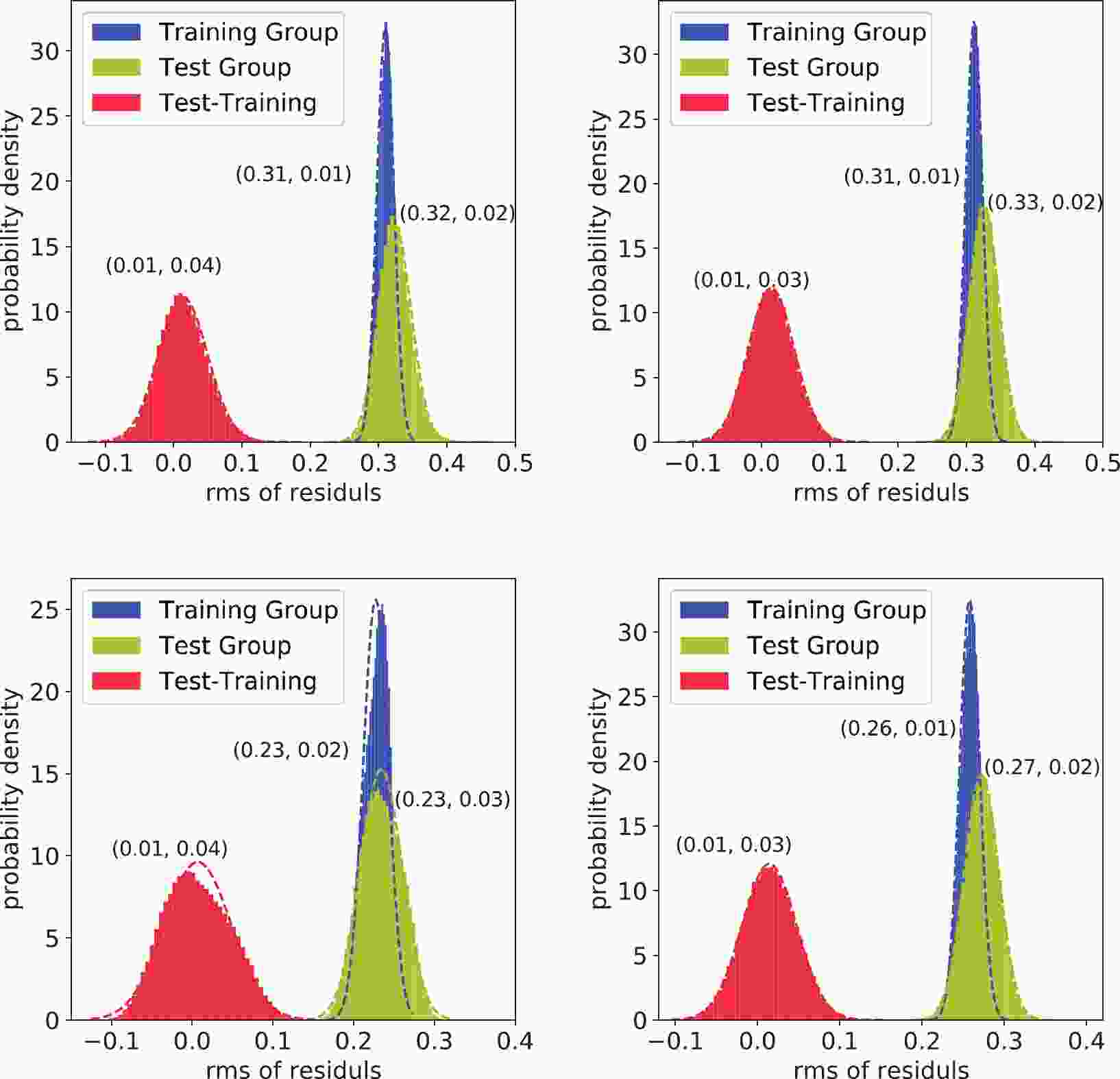
$ n_{i,{\rm tr}} $ ($ n_{i,{\rm ts}} $ ) is the number of nuclides in the training (test) group. In other words,$ \sigma_{\rm tr} $ and$ \sigma_{\rm ts} $ describe the systematic uncertainties of random interpolation and extrapolation. The distribution of the uncertainties of the training and test groups are illustrated in Fig. 1 for the binding energy formulas in Eqs. (3) and (4) and the separation energy formulas in Eqs. (22) and (11).$ \sigma_{\rm tr} $ is located within the distribution of$ \sigma_{\rm ts} $ . Their difference,$ \sigma_{\rm tr}-\sigma_{\rm ts} $ , is located at approximately 0.01.$ \sigma_{\rm ts} $ distributes slightly wider than$ \sigma_{\rm tr} $ ; however, this is not statistically significant. The robustness of the systematic uncertainty estimation can be observed through this check. Note that the statistical uncertainty estimation is restricted to the sub-parameter-space of the correction terms because the uncertainty of the JUN45 interaction is not significant, as discussed later.
Figure 1. (color online) Distribution of the uncertainties of the training group, test group, and their difference. The top two are for Eqs. (3) and (4). The bottom two are for Eqs. (22) and (11). The dashed lines are the fitted normal distributions, the parameters of which, i.e., the mean and standard deviation, are listed in the nearby parentheses.
As for the prediction of the stabilities of p-emission and
$ 2p $ -emission, i.e.,$ P(S_{ p}(Z, N)<0) $ and$ P(S_{ 2p}(Z, N)<0) $ , one could integrate them directly by assuming normalized distributions for the$ S_{ p}(Z, N) $ and$ S_{ 2p}(Z, N) $ energies, which are established from the parameter space of the formula and the corresponding systematic uncertainty.The results of the application on the binding energy formulas Eqs. (2)–(5) and separation energy formulas Eqs. (6)–(11) are presented and discussed in the subsequent section.
-
In this study, experimental data are taken from AME2016 [52] within the nuclear landscape
$ Z, N \in [30,50] $ , corresponding to the$ f_{5}pg_{9} $ shell. Two hundred and twenty-one nuclides with experimentally determined (values without #) binding energies are obtained to perform the preliminary computation. For$ S_ {p} $ and$ S_ {2p} $ , the regions are narrowed to$ Z, N\in [31,50] $ and$ Z, N\in [32,50] $ , respectively, including 198 nuclides with experimentally determined$ S_ {p} $ and 178 nuclides with experimentally determined$ S_ {2p} $ . This choice is to avoid uncertainties introduced by the calculation of nuclides with$ Z, N $ = 28 and 29. Besides these measurements, there are, in principle, 220 nuclides for$ E_{\rm BE} $ , 202 nuclides for S$ _{p} $ , and 183 nuclides for S$ _{2p} $ to be predicted. In practice, it is not necessary to predict all unknown nuclides in the model space because many of them are far beyond the proton dripline. -
The binding energy formulas Eqs. (2)–(5) are applied to the 221 nuclides with measured binding energies via the bootstrap framework. The obtained parameters and uncertainties are summarized in Table 1. As mentioned in Sec. II.A, the effect of the Coulomb interaction is included in the a and b terms. The repulsion between protons will decrease the single particle energy of a proton orbit and the energy released when they form a nucleus, which is consistent with the negative values of a and b. In Eq. (3), the residual is summarized as the competition between the neutron shell effect and isospin effect, which are represented through the square of the valence neutrons and that of the difference between valence protons and neutrons. Because parameters c and d of Eq. (3) are of a similar scale but opposite sign, these two effects compensate for each other when they are far from the proton dripline; this also leads to the equivalence between Eqs. (3) and (4). The large systematic and statistical uncertainties of Eq. (2), which are approximately twice as large as those of the rest, demonstrate the deficiency of Eq. (2). Eq. (5) achieves the best performance regarding the total and systematic uncertainties, but at the price of six parameters, which results in a significant extrapolation weakness. To control the extrapolating uncertainty in the prediction, the consideration of fewer parameters is recommended.
Figure 2 shows the average of the residuals for each nuclide with experimentally determined binding energies evaluated by AME2016 in the region of
$ 30 \leqslant Z{, } N \leqslant50 $ . The values of the residuals are presented by the gradation of color. Starting from white, the redder the color, the more positive the value, and the bluer the color, the more negative the value. No data have residuals larger than$ 3\hat{\sigma}_{\rm total} $ or smaller than$ -3\hat{\sigma}_{\rm total} $ . The extrapolation power is delineated in Fig. 3 by the recomposed uncertainty deduced from Eq. (19). Both formulas exhibit uncertainties that are small near the reached binding energy boundary and increase when moving away. Our predictions for the binding energies are mostly smaller than the extrapolation of AME2016 shown in Table 2. This is consistent with the fact that nuclei near the dripline are less bound than nuclei near the stability line because the extrapolation of AME2016 was obtained under an assumption of a smooth mass surface [53]. Furthermore, more nuclides bound under the energy criterion are predicted in the present study, which awaits experimental examination.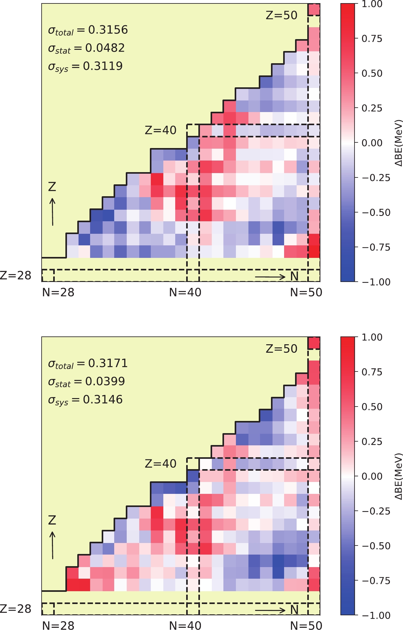
Figure 2. (color online) Distribution of the mean residual of each nuclide for binding energy formulas Eqs. (3) and (4) in order. The dark solid line shows the measurement boundary of the binding energy in AME2016 [52].
Nucl. Eq. (3) Eq. (4) AME2016 Nucl. Eq. (3) Eq. (4) AME2016 Nucl. Eq. (3) Eq. (4) AME2016 Nucl. Eq. (3) Eq. (4) AME2016 62Ge 516.994 517.672 517.142 63As 515.644 516.200 516.159 84Tc 681.878 681.420 682.080 85Tc 698.130 697.735 698.275 64As 529.876 530.363 530.304 64Se 516.288 516.717 516.672 86Tc 712.049 711.722 712.080 82Ru 631.847 631.119 65Se 530.673 531.043 531.050 66Se 547.138 547.453 547.800 83Ru 647.709 647.043 84Ru 666.221 665.622 65Br 513.356 513.653 66Br 528.900 529.148 85Ru 681.555 681.025 682.550 86Ru 698.695 698.238 699.438 67Br 545.496 545.698 546.184 68Br 559.822 559.981 560.252 87Ru 712.819 712.439 713.313 88Ru 729.081 728.781 730.224 66Kr 512.830 512.991 67Kr 528.600 528.720 89Ru 741.323 741.106 742.171 85Rh 662.535 661.849 68Kr 546.273 546.357 69Kr 560.616 560.667 561.177 86Rh 678.669 678.062 87Rh 696.063 695.538 70Kr 577.440 577.462 577.920 69Rb 543.093 543.054 88Rh 711.244 710.805 711.920 89Rh 727.788 727.438 728.999 70Rb 558.518 558.456 71Rb 575.800 575.718 576.165 90Rh 742.871 742.614 742.950 91Rh 757.236 757.076 757.848 72Rb 590.462 590.363 590.544 73Rb 606.793 606.681 606.338 86Pd 661.508 660.732 87Pd 677.532 676.843 70Sr 542.659 542.493 71Sr 558.180 558.000 88Pd 696.041 695.444 89Pd 711.176 710.674 72Sr 576.369 576.178 73Sr 590.968 590.770 591.446 90Pd 729.042 728.639 730.170 91Pd 743.462 743.162 744.471 74Sr 608.019 607.817 608.354 73Y 573.321 573.017 92Pd 760.500 760.305 761.116 93Pd 773.310 773.224 773.667 74Y 588.947 588.644 75Y 606.148 605.851 606.675 89Ag 692.519 691.845 90Ag 708.699 708.130 76Y 621.059 620.771 621.376 77Y 636.978 636.702 637.406 91Ag 726.633 726.172 92Ag 742.292 741.943 742.900 78Y 650.758 650.498 651.222 74Zr 572.619 572.197 93Ag 759.299 759.064 760.089 94Ag 774.707 774.591 774.372 75Zr 588.291 587.879 76Zr 606.415 606.018 95Ag 789.642 789.648 789.640 90Cd 691.561 690.805 77Zr 621.419 621.041 622.237 78Zr 638.355 637.998 639.132 91Cd 707.865 707.223 92Cd 726.644 726.120 79Zr 652.222 651.891 653.093 80Zr 668.167 667.864 668.800 93Cd 742.306 741.903 94Cd 760.402 760.123 761.306 77Nb 603.349 602.848 78Nb 619.281 618.807 95Cd 775.394 775.242 775.865 96Cd 792.748 792.728 792.864 79Nb 636.529 636.086 637.214 80Nb 651.777 651.369 652.080 97Cd 805.940 806.055 805.779 93In 723.213 722.621 81Nb 667.637 667.267 668.088 82Nb 681.565 681.237 681.830 94In 739.896 739.434 95In 757.960 757.632 78Mo 602.231 601.620 79Mo 618.297 617.723 96In 774.172 773.981 774.432 97In 791.454 791.403 791.811 80Mo 636.449 635.916 81Mo 651.571 651.082 652.698 98In 806.975 807.069 806.540 99In 822.625 822.866 822.096 82Mo 668.686 668.245 669.366 83Mo 683.032 682.642 683.422 94Sn 722.013 721.348 95Sn 738.737 738.211 84Mo 698.914 698.578 699.300 81Tc 633.033 632.405 96Sn 757.639 757.257 97Sn 773.837 773.601 82Tc 649.053 648.478 83Tc 666.556 666.038 667.569 98Sn 792.195 792.109 99Sn 807.901 807.968 807.840 Table 2. Comparison of the predicted ground-state binding energies with those in AME2016 [52] for even-Z nuclides with
$ N\geqslant Z-6 $ and odd-Z nuclides with$ N\geqslant Z-5 $ . The unit of energy is MeV.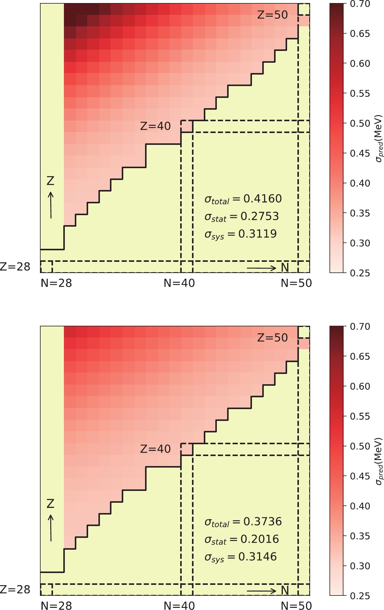
Figure 3. (color online) Distribution of predictive uncertainty of each nuclide for binding energy formulas Eqs. (3) and (4) in order. The dark solid line shows the measurement boundary of the binding energy in AME2016 [52].
We also attempt another interaction, jj44bpn [54], in the same model space; however, this does not perform well for the description of binding energy. As a quick comparison,
$ E_{\rm BE, SM} $ of nuclides with$ 45\leqslant N \leqslant 50 $ or$ 30\leqslant Z\leqslant33 $ is calculated through these two interactions. When applied to Eqs. (2)–(5), jj44bpn still has a larger rms of the residuals compared with JUN45, as presented in Table 3. Because jj44bpn does not provide a better description of the binding energy than JUN45, the corresponding results from jj44bpn are not further discussed in the present study.Eq. (2) Eq. (3) Eq. (4) Eq. (5) JUN45 0.586 0.249 0.292 0.249 jj44bpn 0.722 0.873 0.848 0.700 Table 3. Rms of the residuals when JUN45 and jj44bpn are applied to Eqs. (2)–(5) among nuclides with
$ N \geqslant 45 $ or$ Z \leqslant 33 $ .When constructing the JUN45 interaction, nuclides with
$ N < 46 $ and$ Z > 33 $ are excluded due to their deformations, the description for which the model space may not be sufficient [48]. To investigate and evaluate the description of nuclides in the middle region, the dataset is divided into two parts: 1)$ N < 45 $ &$ Z > 33 $ and 2)$ N \geqslant 45 $ or$ Z \leqslant 33 $ . The bootstrap framework is performed separately on these two subsets. The quantification of the deformation effect originates from a cross-extrapolation estimation. As listed in Table 4, compared with the self-estimated result, the systematic uncertainty of the middle region increases significantly when calculated using the parameters estimated with the outer region, and vice versa. This does reveal the difference between nuclides in these two regions. However, the proposed corrections for Eqs. (3) and (4) lead to a trade-off when the full dataset is considered. The uncertainties of the middle region, estimated by parameters fitted to the entire dataset, deviate by less than 0.08 MeV compared with the self-estimated result. Thus, it is reasonable to describe the nuclides in the middle region through the present framework.Objective region Parameter region $ \sigma_{\rm total} $ *

$ \sigma_{\rm stat} $ *

$ \sigma_{\rm sys} $ *

Eq. (3) Middle Middle 0.317 0.0849 0.305 Outer 0.557 0.0569 0.554 Entire 0.379 0.0437 0.377 Outer Outer 0.254 0.0473 0.250 Middle 0.867 0.305 0.812 Entire 0.286 0.0499 0.281 Eq. (4) Middle Middle 0.327 0.0768 0.317 Outer 0.382 0.0724 0.375 Entire 0.355 0.0431 0.352 Outer Outer 0.295 0.0426 0.292 Middle 0.461 0.153 0.434 Entire 0.300 0.0385 0.298 Table 4. Comparison of the decomposed uncertainties estimated by parameters obtained from the middle region (
$ N < 45 $ &$ Z > 33 $ ), outer region ($ N \geqslant 45 $ or$ Z \leqslant 33 $ ), and entire region. The parameters of Eq. (3) obtained from the middle region are$ a=-9.62 (3) $ ,$ b=-0.0858 (37) $ ,$ c=0.0175 (18) $ , and$ d=-0.0108 (44) $ ; those from the outer region are$ a=-9.53 (2) $ ,$ b=-0.0968 (8) $ ,$ c=0.0229 (5) $ , and$ d=-0.0250 (9) $ . The parameters of Eq. (4) obtained from the middle region are$ a=-9.19 (2) $ ,$ b=-0.0873 (21) $ , and$ c=-0.0276 (13) $ ; those from the outer region are$ a=-9.10 (1) $ ,$ b=-0.0932 (7) $ , and$ c=-0.0305 (7) $ . The parameters obtained from the entire region are taken from Table 1.Random perturbations in the gaussian form with a σ of 20% (
$ \mathcal{N}(x, \sigma=0.2x) $ ) are applied to the 133 two-body matrix elements (TBMEs). If the uncertainty of the JUN45 interaction remains large, a random perturbation would have a significant probability of obtaining better results for the binding energies. The region is narrowed to the 128 nuclides whose total valence particles and holes are less than 13, corresponding to$ A\leqslant 68 $ or$ A\geqslant 88 $ or$ N\geqslant Z+10 $ . Specifically, the application of perturbation to the JUN45 interaction is divided into three groups according to the TBMEs being changed: only the diagonal TBMEs (D), only the non-diagonal TBMEs (ND), and both of these TBMEs (D+ND). Subsequently, the energies relative to the core resulting from the perturbed interactions are inserted into the binding energy formulas to produce a fit, and the rms of the residuals is calculated. For each group, the perturbation is applied 50 times.As listed in Table 5 and shown in Fig. 4, the average of the rms of the residuals is larger than that without perturbation for each binding energy formula. However, the influence of the perturbation applied to the non-diagonal TBMEs is weak because the average of the rms of its residuals only exceeds that of the unperturbed one at approximately 0.07 MeV and its distribution is narrow, as illustrated in Fig. 4.

Figure 4. (color online) Distribution of the rms of the residuals and the number of consistent
$ J^\pi $ for perturbations applied to the JUN45 interaction. The dashed lines are the fitted normal distributions, the parameters of which, i.e., the mean and standard deviation, are listed in the nearby parentheses. The vertical black solid line denotes the value when no perturbation is applied, and the black number in parentheses is its corresponding value.Eq. (2) Eq. (3) Eq. (4) Eq. (5) JUN45 0.651 0.219 0.292 0.216 D 0.778 (201) 0.580 (236) 1.119 (421) 0.464 (159) ND 0.680 (57) 0.290 (58) 0.359 (62) 0.259 (36) D+ND 0.787 (181) 0.638 (241) 0.979 (388) 0.505 (148) Table 5. Comparison of the rms of the residuals when no perturbation is applied to the JUN45 interaction with the average and standard deviation of the rms of the residuals when perturbation is applied to D, ND, and D+ND of the JUN45 interaction among nuclides whose number of valence particles and holes is less than 13.
The rms is sensitive to the diagonal TBMEs, as shown through the wide expansion of the distribution in case D and D+ND. Moreover, the rms of the residuals without perturbation drops out of 1.5 (1.75) σ of the distribution when perturbation is applied to the diagonal (all) TBMEs, which implies the significant influence of perturbation and the well fitted diagonal TBMEs of JUN45 interaction. In addition, the number of nuclides, whose spin and parity (
$ J^\pi $ ) resulting from the perturbed interaction are consistent with those from the observation, is counted. The distribution of the consistency is illustrated in the right panel of Fig. 4. This shows similar results to the perturbation cases for rms. Therefore, the uncertainty of the JUN45 interaction in the energy calculation is shown to be insignificant without perturbation.The spin and parity of the ground state calculated by the JUN45 interaction (
$ J^\pi_{\rm{JUN45}} $ ) are also compared with those ($ J^\pi_{\rm exp} $ ) from the NNDC. Among the 198 nuclides with determined$ J^\pi_{\rm exp} $ , there are 137 nuclides whose$ J^\pi_{\rm{JUN45}} $ is consistent with$ J^\pi_{\rm exp} $ . Moreover, there are 54 nuclides with undetermined$ J^\pi_{\rm exp} $ . This rarely influences the description of the absolute value of binding energy, which is a bulk property of the nucleus. Generally, nuclear mass models, e.g., the developed semi-empirical droplet model [12, 13], finite-range droplet model [14−19], and application of Hartree-Fock-Bogoliubov theory [20, 21], do not concentrate on the spin and parity. -
Because Eqs. (3) and (4) exhibit good agreement with the experimental binding energies, the deduced formulas are accordingly investigated for the separation energies of the last proton and last two protons, which are expressed by Eqs. (6)−(11). The bootstrap framework is directly applied to the separation energy formulas rather than calculating the separation energies using the binding energy formulas, which can avoid error propagation. Eqs. (6), (8), and (10) and Eqs. (7), (9), and (11) are applied to the 198
$ S_ {p} $ and 178$ S_ {2p} $ evaluated in AME2016, respectively.The fitting values of the parameters a, c, and d of the
$ S_ {2p} $ formulas are almost a factor of two larger than those of the corresponding parameters for the$ S_ {p} $ formulas. This approximated double relation is mainly caused by the nature of subtracting two protons and one proton in the calculation of$ S_ {2p} $ and$ S_ {p} $ , respectively. Eq. (10) tends to overestimate odd-Z nuclides but underestimate even-Z nuclides, which indicates that the pairing strength may not be well described in shell-model calculations. It is beneficial to introduce an estimation for such extra energy as$ \begin{aligned}[b] S_ {p}(Z, N)=&E_{\rm BE, SM}(Z, N) - E_{\rm BE, SM}(Z-1, N) \\ & + aZ + c(Z-N)^{2} + d + e\delta_{Z}, \end{aligned} $

(22) where
$ \delta_{Z}=0 $ if Z is even and$ \delta_{Z}=1 $ if Z is odd. The correction reduces the uncertainty, as listed in Table 1, and smoothens the residual distribution, as shown in Fig. 5.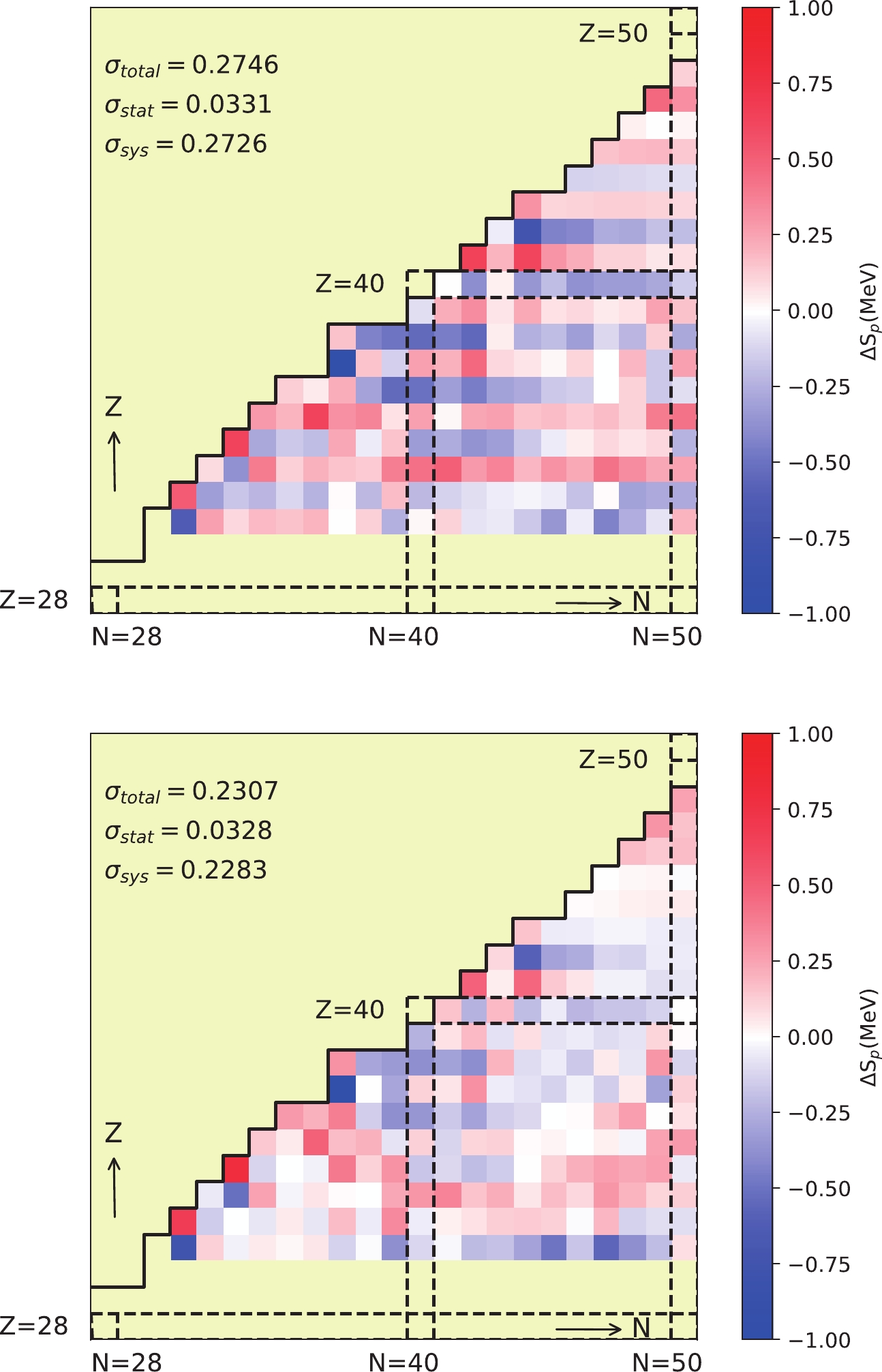
Figure 5. (color online) Distribution of the mean residual of each nuclide for the
$ S_{p} $ formulas Eqs. (10) and (22) in order.Beyond the proton(s) boundary discovered experimentally in AME2016, the separation energies are also calculated theoretically. Figs. 6 and 7 compare the values of
$ S_{p} $ and$ S_{2p} $ , respectively, calculated through Eqs. (22) and (11) and those of AME2016. The calculated values agree well with the experimental data, which are mostly located within the 2σ range of the calculations. The present calculations generally agree with the extrapolated values in AME2016, but with smaller uncertainties. This provides important inputs for simulations in nuclear astrophysics and has a significant impact on the understanding of p-process nuclei and their solar abundance. This is because the$ S_p $ taken by Pruet$ et \ al. $ for the$ \nu p $ -process reaction flow through the Zn-Sn regions for exploring the production of p nuclei in neutrino-driven wind from a young neutron star in Type II supernovae [55] has an extremely large extrapolated uncertainty. They found that the synthesis of p-rich nuclei could be reached up to 102Pd, although their calculations did not reveal efficient production of 92Mo. If the entropy of these ejecta were increased by a factor of 2, the synthesis could extend to 120Te. Further increases in entropy, which might reflect the role of magnetic fields or the vibrational energy input neglected in the hydrodynamical model, resulted in the production of nuclei up to$ A\approx170 $ .
Figure 6. (color online)
$ S_ {p} $ calculated in this study and that determined and extrapolated in AME2016.$ S_ {p, {\rm cal}} $ are the values calculated using Eq. (22),$ S_ {p, {\rm exp}} $ are the values determined experimentally in AME2016, and$ S_ {p, {\rm AME}} $ are the extrapolated values in AME2016. The green region, red error bars, and blue region denote the 2σ uncertainties for$ S_ {p,{\rm cal}} $ ,$ S_ {p,{\rm exp}} $ , and$S_ {p,{\rm AME}}$ , respectively.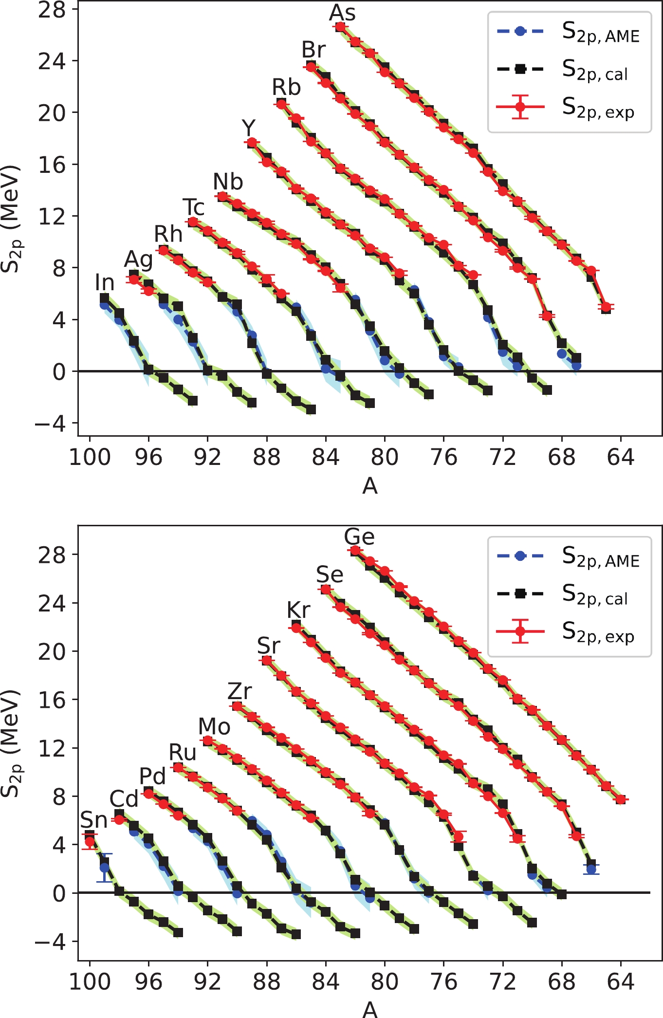
Figure 7. (color online)
$ S_ {2p} $ calculated in this study and that determined and extrapolated in AME2016. See similar caption of Fig. 6.For the isotope chains of Ge, As, Se, Br, Kr, and Sr, the observed
$ S_ {p} $ decreases sharply when Z exceeds N. Both the extrapolations in the present study and in AME2016 present such characteristics for other isotopes. For odd-Z nuclides (top of Fig. 6), such a gap leads to the single proton dripline, whereas the pairing of protons makes the single proton dripline of even-Z nuclides farther to reach. This phenomenon also exists for$ S_ {2p} $ , as shown in Fig. 7. A sharp decrease is shown for As, Se, Br, Kr, and Sr and predicted for other isotopes when Z exceeds N but is smoothed because of the correlation between the two emitted protons. Thus, the proton dripline tends to be extended beyond the$ Z=N $ line by the competition between the pairing of protons and$ Z/N $ symmetry.The resampling process in the bootstrap framework estimates the parameter space of Eqs. (22) and (11). Simultaneously, it also estimates the distribution of
$ S_ p $ and$ S_{ 2p} $ for each nuclide. Hence, the possibilities of$ S_{ p}<0 $ and$ S_{ 2p}<0 $ for each nuclide are obtained by integrating the estimated normalized distribution. As listed in Table 6, the p- and 2p- driplines are predicted based on the present calculations.Nucl. $ l_{p} $ 

$ S_{ p} /{\rm{ MeV}}$ 

$ P (S_{ p} < 0) $ 

$ \log_{10}T_{\rm cal} $ 

$ \log_{10}T_{\rm exp} $ 

$ l_{2p} $ 

$ S_{ 2p}/{\rm{ MeV}} $ 

$ P (S_{ 2p} < 0) $ 

$ \log_{10}T_{\rm cal} $ 

64As 1 −0.157 75% $ 8.6_{-18.2} $ 

65Se 1.244 0% 66Se 2.460 0% 2.352 0% 66Br 1 −1.545 100% $ -15.8_{-1.5}^{+2.4} $ 

67Br $ ^{\rm \#} $ 

1 −1.491 100% $ -15.6_{-1.6}^{+2.6} $ 

1.019 0% 68Br $ ^{\rm \#} $ 

1 −0.540 99% $ -7.3_{-5.6}^{+33.9} $ 

−7.3 [62] 2.142 0% 67Kr 0.321 8% 68Kr 1.312 0% −0.117 67% 69Kr 1.252 0% 0.767 0% 70Kr 2.465 0% 2.016 0% 69Rb 3 −2.856 100% $ -16.9_{-0.7}^{+0.9} $ 

2 −1.468 100% $ 2.7_{-5.2}^{+9.1} $ 

70Rb 1 −1.859 100% $ -15.5_{-1.3}^{+1.8} $ 

2 −0.539 98% $ 26.6_{-17.5}^{+319.2} $ 

71Rb $ ^{\rm \#} $ 

3 −1.479 100% $ -13.1_{-1.7}^{+2.7} $ 

1.047 0% 72Rb 1 −0.491 98% $ -5.2_{-6.6}^{+70.1} $ 

$ -7.0_{-0.1}^{+0.08} $ [59]

2.038 0% 73Rb 1 −0.285 89% $ 2.1_{-11.7} $ 

<-7.1 [59] 4.695 0% 70Sr 0.290 10% 0 −2.477 100% $ -5.7_{-2.6}^{+3.7} $ 

71Sr 0.294 10% 0 −1.485 100% $ 2.8_{-5.3}^{+9.1} $ 

72Sr 1.115 0% 0 −0.290 87% $ 50.2_{-34.3} $ 

73Sr 0.975 0% 0.550 2% 74Sr 1.624 0% 1.397 0% 73Y 4 −2.712 100% $ -14.9_{-0.8}^{+1.0} $ 

3 −1.511 100% $ 4.4_{-5.3}^{+9.1} $ 

74Y 2 −1.771 100% $ -15.0_{-1.4}^{+2.1} $ 

1 −0.717 100% $ 20.7_{-13.3}^{+51.7} $ 

75Y 2 −1.698 100% $ -14.7_{-1.5}^{+2.3} $ 

−0.003 51% 76Y $ ^{\rm \#} $ 

0 −0.752 100% $ -9.2_{-4.2}^{+12.0} $ 

1.613 0% 77Y 2 −0.520 99% $ -4.1_{-6.5}^{+46.1} $ 

3.568 0% 78Y 1.653 0% 5.980 0% 74Zr 0.033 44% 0 −2.580 100% $ -5.1_{-2.6}^{+3.6} $ 

75Zr −0.014 52% 2 −1.693 100% $ 2.5_{-4.7}^{+7.6} $ 

76Zr 0.825 0% 0 −0.790 100% $ 19.2_{-12.2}^{+39.6} $ 

77Zr 0.840 0% 0.165 26% 78Zr 1.786 0% 1.335 0% 79Zr 1.810 0% 3.525 0% 80Zr 3.887 0% 5.634 0% 77Nb 2 −2.720 100% $ -17.2_{-0.8}^{+1.1} $ 

0 −1.798 100% $ 1.6_{-4.4}^{+7.0} $ 

78Nb 1 −1.878 100% $ -15.6_{-1.4}^{+2.0} $ 

1 −0.948 100% $ 15.7_{-10.0}^{+25.4} $ 

79Nb 1 −1.643 100% $ -14.7_{-1.6}^{+2.5} $ 

0.225 20% 80Nb 1 −0.332 93% $ 2.5_{-11.1} $ 

1.553 0% 81Nb 1 −0.480 98% $ -2.8_{-7.5}^{+101.3} $ 

<−7.4 [63] 3.475 0% 82Nb 1.336 0% 5.150 0% Continued on next page Table 6. Predicted
$ S_ p $ and$ S_{ 2p} $ and the possibility of negative$ S_ p $ and$ S_{ 2p} $ for experimentally undetermined nuclides, respectively. The partial half-lives, in units of seconds, are calculated for nuclides with$ P>70\% $ using Eq. (23). The half-lives of several ground state nuclides determined experimentally are also listed. Nuclides that are unstable but bound against both p-emission and 2p-emission are marked in bold. Those predicted to be pure p-emitters and pure 2p-emitters are marked with$ ^\# $ and$ ^\dagger $ , respectively.Thirty candidates that are unstable but bound against both p-emission and 2p-emission are predicted in Table 6 under the condition of
$ P(S_{ p}<0)<1\% \cap P(S_{ 2p}<0)<1\% $ , which are marked in bold in Table 6. Note that$ ^{100}_{50} $ Sn is experimentally$ S_{ 2p} $ known and bound. The present calculation suggests that the drip-lines pass over the$ Z=N $ line in this region, which may provide new ideas for waiting points in the path of nucleosynthesis. The separation energies and binding probabilities also provide an opportunity to estimate the pure p-emitters and pure$ 2p $ -emitters in the region$ Z,N\in [32,50] $ . Under the conditions$ P(S_{ p}<0)> 99\% \;\cap P(S_{ 2p}<0)<1\% $ and$ P(S_{ p}<0)<1\% \cap P(S_{ 2p}<0)> 99\% $ , nine nuclides (marked with$ ^\# $ ) and three nuclides (marked with$ ^\dagger $ ) are predicted to be pure p-emitters and pure$ 2p $ -emitters, respectively.Table 6-continued from previous page Nucl. $ l_{p} $ 

$ S_p /{\rm{ MeV}}$ 

$ P (S_{ p} < 0) $ 

$ \log_{10}T_{\rm cal} $ 

$ \log_{10}T_{\rm exp} $ 

$ l_{ 2p} $ 

$ S_{ 2p}/{\rm{ MeV}} $ 

$ P (S_{ 2p} < 0) $ 

$ \log_{10}T_{\rm cal} $ 

78Mo 2 −0.372 95% $ 2.19_{-10.1} $ 

0 −2.982 100% $ -6.1_{-2.3}^{+3.0} $ 

79Mo 2 −0.330 92% $ 4.1_{-11.4} $ 

1 −2.105 100% $ -0.3_{-3.7}^{+5.4} $ 

80Mo 0.489 2% 0 −1.059 100% $ 13.9_{-9.1}^{+20.2} $ 

81Mo 0.284 11% 0.040 44% 82Mo 1.469 0% 1.069 0% 83Mo 1.824 0% 3.234 0% 84Mo 3.360 0% 5.131 0% 81Tc 1 −3.059 100% $ -18.2_{-0.7}^{+0.9} $ 

2 −2.462 100% $ -2.0_{-3.1}^{+4.2} $ 

82Tc 2 −2.246 100% $ -15.7_{-1.1}^{+1.5} $ 

3 −1.861 100% $ 3.5_{-4.5}^{+6.9} $ 

83Tc 1 −1.936 100% $ -15.4_{-1.4}^{+2.0} $ 

2 −0.373 92% $ 50.1_{-30.4} $ 

84Tc $ ^{\rm \#} $ 

2 −1.031 100% $ -9.7_{-3.2}^{+6.5} $ 

0.879 0% 85Tc $ ^{\rm \#} $ 

1 −0.724 100% $ -6.7_{-4.9}^{+14.7} $ 

<−7.4 [63] 2.714 0% 86Tc 0.863 0% 4.616 0% 82Ru 1 −0.429 97% $ 0.6_{-9.1} $ 

0 −3.367 100% $ -6.8_{-2.1}^{+2.6} $ 

83Ru 4 −0.679 100% $ -2.5_{-5.4}^{+18.1} $ 

2 −2.812 100% $ -3.6_{-2.6}^{+3.5} $ 

84Ru 0.244 14% 0 −1.586 100% $ 6.5_{-5.7}^{+9.5} $ 

85Ru 0.179 22% 2 −0.754 100% $ 26.1_{-14.4}^{+51} $ 

86Ru 0.996 0% 0.364 8% 87Ru 1.138 0% 2.085 0% 88Ru 3.276 0% 4.372 0% 89Ru 3.509 0% 5.613 0% 85Rh 4 −3.318 100% $ -15.3_{-0.7}^{+0.9} $ 

3 −2.955 100% $ -3.3_{-2.5}^{+3.3} $ 

86Rh 2 −2.603 100% $ -16.3_{-1.0}^{+1.3} $ 

6 −2.313 100% $ 3.3_{-3.5}^{+5.0} $ 

87Rh 4 −2.427 100% $ -13.5_{-1.1}^{+1.4} $ 

3 −1.327 100% $ 12.3_{-7.3}^{+13.8} $ 

88Rh 0 −1.441 100% $ -13.0_{-2.2}^{+3.5} $ 

6 −0.206 78% $ 87.9_{-56.7} $ 

89Rh $ ^{\rm \#} $ 

4 −1.223 100% $ -4.6_{-2.7}^{+4.8} $ 

<−6.9 [58] 2.143 0% 90Rh 1.563 0% 5.154 0% 91Rh 0.851 0% 5.716 0% 86Pd 4 −0.259 87% $ 13.7_{-16.1} $ 

0 −3.445 100% $ -6.2_{-2.1}^{+2.7} $ 

87Pd 5 −0.462 98% $ 5.3_{-8.8} $ 

5 −2.940 100% $ -1.2_{-2.6}^{+3.4} $ 

88Pd $ ^{\rm \dagger} $ 

0.568 1% 0 −1.742 100% $ 6.1_{-5.3}^{+8.4} $ 

89Pd 0.444 3% 0 −0.887 100% $ 23.1_{-12.4}^{+34.4} $ 

90Pd 1.696 0% 0.575 1% 91Pd 0.970 0% 2.628 0% 92Pd 3.587 0% 4.526 0% 93Pd 3.507 0% 5.636 0% 89Ag 4 −3.143 100% $ -14.8_{-0.8}^{+1.0} $ 

2 −2.445 100% $ 0.6_{-3.5}^{+4.8} $ 

90Ag 4 −2.183 100% $ -12.4_{-1.3}^{+1.8} $ 

4 −1.616 100% $ 10.1_{-5.9}^{+10} $ 

91Ag 4 −2.192 100% $ -12.5_{-1.3}^{+1.8} $ 

0 −0.381 92% $ 56.3_{-32.9} $ 

92Ag 2 −1.024 100% $ -8.2_{-3.5}^{+7.2} $ 

0.053 42% 93Ag $ ^{\rm \#} $ 

4 −1.119 100% $ -6.9_{-3.1}^{+6.0} $ 

$ -6.6_{-0.03}^{+0.03} $ [58]

2.568 0% Continued on next page Table 6-continued from previous page Nucl. $l_{p}$ 

$ S_{ p}/{\rm{ MeV}}$ 

$ P (S_{ p} < 0) $ 

$ \log_{10}T_{\rm cal} $ 

$ \log_{10}T_{\rm exp} $ 

$ l_{ 2p} $ 

$ S_{{\boldsymbol{}}2p}/{\rm{ MeV}} $ 

$ P (S_{ 2p} < 0) $ 

$ \log_{10}T_{\rm cal} $ 

94Ag 1.423 0% 5.023 0% 95Ag 0.958 0% 5.598 0% 90Cd 4 −0.179 78% $ 23.6_{-23.8} $ 

0 −3.180 100% $ -3.9_{-2.4}^{+3.2} $ 

91Cd 4 −0.147 74% $ 28.8_{-28.3} $ 

0 −2.195 100% $ 2.8_{-4.1}^{+5.9} $ 

92Cd $ ^{\rm \dagger} $ 

0.612 0% 0 −1.453 100% $ 11.9_{-7.1}^{+12.5} $ 

93Cd 0.537 1% 0 −0.367 92% $ 60.1_{-35.1} $ 

94Cd 1.556 0% 0.550 2% 95Cd 1.076 0% 2.605 0% 96Cd 3.439 0% 4.495 0% 97Cd 3.317 0% 5.545 0% 93In 4 −3.041 100% $ -14.3_{-0.9}^{+1.1} $ 

0 −2.288 100% $ 2.7_{-4.0}^{+5.6} $ 

94In 0 −2.105 100% $ -15.0_{-1.4}^{+2.0} $ 

2 −1.435 100% $ 13.5_{-7.3}^{+13.2} $ 

95In 4 −2.215 100% $ -12.2_{-1.3}^{+1.8} $ 

0 −0.533 98% $ 45.1_{-24.1} $ 

96In 4 −1.065 100% $ -5.8_{-3.5}^{+7.0} $ 

0.130 31% 97In $ ^{\rm \#} $ 

4 −1.201 100% $ -7.0_{-3.0}^{+5.5} $ 

2.349 0% 98In 1.072 0% 4.494 0% 99In 1.207 0% 5.657 0% 94Sn 4 −0.410 96% $ 7.8_{-11} $ 

0 −3.297 100% $ -3.4_{-2.5}^{+3.1} $ 

95Sn 0 −0.462 98% $ 2.6_{-9.6} $ 

0 −2.421 100% $ 2.2_{-3.8}^{+5.3} $ 

96Sn 0.291 11% 0 −1.785 100% $ 8.7_{-5.7}^{+8.9} $ 

97Sn 0.199 20% 0 −0.735 100% $ 34.2_{-17.1}^{+66.4} $ 

98Sn 1.205 0% 0.128 32% 99Sn 1.326 0% 2.515 0% 100Sn 3.474 0% With the assumption that the emission is dominated by the channel from ground state to ground state and ignoring the deformation, the corresponding decay half-lives are calculated using a simple law proposed by Qi et al. [56]:
$ \begin{array}{*{20}{l}} \log_{10} T_{1/2} = a\chi'+b\rho'+dl(l+1)/\rho'+c, \end{array} $

(23) where
$ \chi'=Z_{p}Z_{d}\sqrt{X/Q_{p}} $ ,$ \rho'=\sqrt{XZ_{p}Z_{d}(A_{p}^{1/3}+A_{d}^{1/3})} $ , and$ X = A_{p}A_{d}/(A_{p}+A_{d}) $ . The subscripts p and d denote a proton and daughter nucleus, respectively. The parameters are refit to be$ a=0.4559,\; b=-0.4272,\; d=2.5706, \;c=-23.08 $ based on the data for nuclides with$ N < 75 $ taken from Ref. [56]. Here, 130Eu and 112Cs are removed because of their large experimental uncertainty and undetermined angular momentum. The uncertainty of separation energy within the$ 2\sigma $ range is accounted for, which denotes a 95% confidence interval. The experimentally determined$ J^\pi_{g.s.} $ is taken in the partial half-life prediction. If the experimental data is not available,$ J^\pi_{g.s.} $ of its mirror partner is used, which is a feasible choice. To the best of our knowledge, there is only one observed mirror-symmetry-violated case for$ J^\pi_{g.s.} $ [57]. If the$ J^\pi_{g.s.} $ values of both mirror partners are unknown, the calculated values are used for a referenced estimation.In recent years, several nuclides in this region have been identified via experiments. Although several nuclides have not been discovered, the limit of their partial half-lives could be estimated. The experimentally estimated ranges of the half-lives of 68Br,
$ ^{72,73} $ Rb, 81Nb, 85Tc, 89Rh, and 93Ag are summarized in Table 6. These are consistent with the calculated values.$ ^{93}_{47} $ Ag$ _{46} $ and$ ^{89}_{45} $ Rh$ _{44} $ have been measured to be one-proton emitters but against two proton emission [58], which is qualitatively consistent with the extrapolation results presented in Table 6.In 2017, the proton emission from the ground-state of 72Rb was measured for the first time [59]. In this study, it is predicted to be proton unbound but two proton bound. Recently, the proton decay of 72Rb was explained by the lower deformation and lower angular momentum barrier [60]. This is consistent with the present calculation under 95% confidence intervals. Its isotope, 73Rb, has not yet been directly measured; however, the upper limit of its half-life was deduced [59]. For 73Rb, the calculated partial half-life has been located beyond the experimental upper limit to date; however, the lower limit estimated theoretically is consistent with this. This is because the calculated
$ S_ {p} $ value in this study is small with large uncertainties, which induces large uncertainties on the predicted partial half-life.76Y was identified in Ref. [60]. The
$ \beta^{+} $ decay with a partial half-life of a few ms was measured as the predominant mode of 76Y, which suggests that this nuclide is possibly proton bound or acquires a sufficiently small proton decay width [60]. In contrast, 76Y is predicted to be proton unbound in the present study, as shown in Table 6. A similar conclusion was drawn in another calculation performed by Kaneko et al. [61].For
$ ^{68}_{35} $ Br, its existence was discovered recently, and its half-life was estimated to be 50 ns [62]. This is consistent with the partial half-life estimated in this study. We suggest further investigations on one proton emitters of 68Br. -
In summary, based on the nuclear shell model, two formulas with four and three terms, respectively, are recommended to calculate the nuclear binding energies using shell-model binding energies in the
$ 30\leqslant Z, N\leqslant50 $ region. The contributions of the Coulomb interaction, neutron shell effect, and isospin effect are effectively included. After applying the bootstrap framework, these two formulas have a total uncertainty of approximately 0.3 MeV for nuclides with experimentally known binding energies. The repulsion characteristic of the Coulomb interaction decreases the binding energy as expected. It is found that the neutron shell effect and isospin effect compensate for each other when they are far from the proton dripline. For those without experimental values, the uncertainty of the predicted data is assessed to be approximately 0.4 MeV, which reveals good extrapolation power. In addition, the formulas for$ S_{ p} $ and$ S_{ 2p} $ are also recommended with uncertainties less than 0.3 MeV. This shows that the predicted uncertainties of the proton(s) separation energies are mostly smaller than those of the AME2016 extrapolations, and the proton dripline can be extended compared with the boundary reached in experiments. The bootstrap method is developed to estimate the possibilities of the proton(s)-emissions$ P(S_{ p}<0) $ and$ P(S_{ 2p}<0) $ from the distribution of$ S_{ p} $ and$ S_{ 2p} $ . The prediction of the proton(s)-emission property of the nuclides is mostly consistent with the experimental results. Thirty nuclides are suggested to be bound against both p-emission and$ 2p $ -emission. Their spectroscopic properties, such as the β-decay spectrum, must be investigated experimentally and theoretically in future. The energies and partial half-lives predicted in this study can be used as inputs for the simulation of nuclear astrophysics. -
We are grateful for the computational resources from SYSU and the National Supercomputer Center in Guangzhou.
Shell-model study on properties of proton dripline nuclides with Z, N = 30–50 including uncertainty analysis
- Received Date: 2022-01-17
- Available Online: 2022-08-15
Abstract: The binding and proton separation energies of nuclides with


 DownLoad: